The Dantzig selector: statistical estimation

when p is much larger than n

Emmanuel Candes† and Terence Tao]

† Applied and Computational Mathematics, Caltech, Pasadena, CA 91125

] Department of Mathematics, University of California, Los Angeles, CA 90095

May 2005; Revised version

Abstract

In many important statistical applications, the number of variables or parameters pis much larger than the number of observations n. Suppose then that we have observa-tions y = Xβ + z, where β ∈ Rp is a parameter vector of interest, X is a data matrixwith possibly far fewer rows than columns, n � p, and the zi’s are i.i.d. N(0, σ2). Is itpossible to estimate β reliably based on the noisy data y?

To estimate β, we introduce a new estimator—we call the Dantzig selector—whichis solution to the `1-regularization problem

minβ∈Rp

‖β‖`1 subject to ‖X∗r‖`∞ ≤ (1 + t−1)√

2 log p · σ,

where r is the residual vector y − Xβ and t is a positive scalar. We show that ifX obeys a uniform uncertainty principle (with unit-normed columns) and if the trueparameter vector β is sufficiently sparse (which here roughly guarantees that the modelis identifiable), then with very large probability

‖β − β‖2`2 ≤ C2 · 2 log p ·

(σ2 +

∑i

min(β2i , σ2)

).

Our results are nonasymptotic and we give values for the constant C. Even though nmay be much smaller than p, our estimator achieves a loss within a logarithmic factorof the ideal mean squared error one would achieve with an oracle which would supplyperfect information about which coordinates are nonzero, and which were above thenoise level.

In multivariate regression and from a model selection viewpoint, our result saysthat it is possible nearly to select the best subset of variables, by solving a very simpleconvex program, which in fact can easily be recast as a convenient linear program (LP).

Keywords. Statistical linear model, model selection, ideal estimation, oracle inequali-ties, sparse solutions to underdetermined systems, `1-minimization, linear programming,restricted orthonormality, geometry in high dimensions, random matrices.

Acknowledgments. E. C. is partially supported in part by a National Science Foundationgrant DMS 01-40698 (FRG) and by an Alfred P. Sloan Fellowship. T. T. is supported inpart by a grant from the Packard Foundation. E. C. thanks Rob Nowak for sending him

1

an early preprint, Hannes Helgason for bibliographical research on this project, JustinRomberg for his help with numerical simulations, and Anestis Antoniadis for comments onan early version of the manuscript. We also thank the referees for their helpful remarks.

1 Introduction

In many important statistical applications, the number of variables or parameters p is nowmuch larger than the number of observations n. In radiology and biomedical imaging forinstance, one is typically able to collect far fewer measurements about an image of inter-est than the unknown number of pixels. Examples in functional MRI and tomography allcome to mind. High dimensional data frequently arise in genomics. Gene expression studiesare a typical example: a relatively low number of observations (in the tens) is available,while the total number of gene assayed (and considered as possible regressors) is easilyin the thousands. Other examples in statistical signal processing and nonparametric es-timation include the recovery of a continuous-time curve or surface from a finite numberof noisy samples. Estimation in this setting is generally acknowledged as an importantchallenge in contemporary statistics, see the recent conference held in Leiden, The Nether-lands (September 2002) “On high-dimensional data p � n in mathematical statistics andbio-medical applications.” It is believed that progress may have the potential for impactacross many areas of statistics [Kettering, Lindsay and Siegmund (2003)].

In many research fields then, scientists work with data matrices with many variables p andcomparably few observations n. This paper is about this important situation, and considersthe problem of estimating a parameter β ∈ Rp from the linear model

y = Xβ + z; (1.1)

y ∈ Rn is a vector of observations, X is an n×p predictor matrix, and z a vector of stochasticmeasurement errors. Unless specified otherwise, we will assume that z ∼ N(0, σ2In) is avector of independent normal random variables, although it is clear that our methods andresults may be extended to other distributions. Throughout this paper, we will of coursetypically assume that p is much larger than n.

1.1 Uniform uncertainty principles and the noiseless case

At first, reliably estimating β from y may seem impossible. Even in the noiseless case, onemay wonder how one could possibly do this as one would need to solve an underdeterminedsystem of equations with fewer equations than unknowns. But suppose now that β is knownto be structured in the sense that it is sparse or compressible. For example, suppose thatβ is S-sparse so that only S of its entries are nonzero. This premise radically changesthe problem, making the search for solutions feasible. In fact, Candes and Tao (2005)showed that in the noiseless case, one could actually recover β exactly by solving the convexprogram1 (‖β‖`1 :=

∑pi=1 |βi|)

(P1) minβ∈Rp

‖β‖`1 subject to Xβ = y, (1.2)

1(P1) can even be recast as a linear program [Chen, Donoho and Saunders (1999)].

2

provided that the matrix X ∈ Rn×p obeys a uniform uncertainty principle. That is, `1-minimization finds without error both the location and amplitudes—which we emphasizeare a-priori completely unknown—of the nonzero components of the vector β ∈ Rp. Wealso refer the reader to Donoho and Huo (2001), Elad and Bruckstein (2002) and Fuchs(2004) for inspiring early results.

To understand the exact recovery phenomenon, we introduce the notion of uniform uncer-tainty principle (UUP) proposed in Candes and Tao (2004) and refined in Candes and Tao(2005). This principle will play an important role throughout although we emphasize thatthis paper is not about the exact recovery of noiseless data. The UUP essentially statesthat the n× p measurement or design matrix X obeys a “restricted isometry hypothesis.”Let XT , T ⊂ {1, . . . , p} be the n × |T | submatrix obtained by extracting the columns ofX corresponding to the indices in T ; then Candes and Tao (2005) define the S-restrictedisometry constant δS of X which is the smallest quantity such that

(1− δS) ‖c‖2`2 ≤ ‖XT c‖2

`2 ≤ (1 + δS) ‖c‖2`2 (1.3)

for all subsets T with |T | ≤ S and coefficient sequences (cj)j∈T . This property essentiallyrequires that every set of columns with cardinality less than S approximately behaves likean orthonormal system. It was shown (also in Candes and Tao (2005)) that if S obeys

δS + δ2S + δ3S < 1, (1.4)

then solving (P1) recovers any sparse signal β with support size obeying |T | ≤ S.

Actually, Candes and Tao (2005) derived a slightly stronger result. Introduce the S, S′-restricted orthogonality constants θS,S′ for S + S′ ≤ p to be the smallest quantity suchthat

|〈XT c,XT ′c′〉| ≤ θS,S′ · ‖c‖`2 ‖c′‖`2 (1.5)

holds for all disjoint sets T, T ′ ⊆ {1, . . . , p} of cardinality |T | ≤ S and |T ′| ≤ S′. Smallvalues of restricted orthogonality constants indicate that disjoint subsets of covariates spannearly orthogonal subspaces. Then the authors showed that the recovery is exact provided

δS + θS,S + θS,2S < 1, (1.6)

which is a little better since it is not hard to see that δS+S′− δS′ ≤ θS,S′ ≤ δS+S′ for S′ ≥ S[Candes and Tao (2005, Lemma 1.1)].

1.2 Uniform uncertainty principles and statistical estimation

Any real-world sensor or measurement device is subject to at least a small amount of noise.And now one asks whether it is possible to reliably estimate the parameter β ∈ Rp fromthe noisy data y ∈ Rn and the model (1.1). Frankly, this may seem like an impossible task.How can one hope to estimate β, when in addition to having too few observations, theseare also contaminated with noise?

To estimate β with noisy data, we consider nevertheless solving the convex program

(DS) minβ∈Rp

‖β‖`1 subject to ‖X∗r‖`∞ := sup1≤i≤p

|(X∗r)i| ≤ λp · σ (1.7)

3

for some λp > 0, and where r is the vector of residuals

r = y −Xβ. (1.8)

In other words, we seek an estimator β with minimum complexity (as measured by the `1-norm) among all objects that are consistent with the data. The constraint on the residualvector imposes that for each i ∈ {1, . . . , p}, |(X∗r)i| ≤ λp · σ, and guarantees that theresiduals are within the noise level. As we shall see later, this proposal makes sense providedthat the columns of X have the same Euclidean size and in this paper, we will always assumethey are unit-normed; our results would equally apply to matrices with different columnsizes—one would only need to change the right hand-side to |(X∗r)i| less or equal to λp · σtimes the Euclidean norm of the ith column of X, or to |(X∗r)i| ≤

√1 + δ1 · λp · σ since all

the columns have norm less than√

1 + δ1.

There are many reasons why one would want to constrain the size of the correlated residualvector X∗r rather than the size of the residual vector r. Suppose that an orthonormaltransformation is applied to the data, giving y′ = Uy where U∗U is the identity. Clearly, agood estimation procedure for estimating β should not depend upon U (after all, one couldapply U∗ to return to the original problem). It turns out that the estimation procedure(1.7) is actually invariant with respect to orthonormal transformations applied to the datavector since the feasible region is invariant: (UX)∗(UXβ−Uy) = X∗(Xβ−y). In contrast,had we defined the feasibility region with supi |ri| being smaller than a fixed threshold, thenthe estimation procedure would not be invariant. There are other reasons aside from this.One of them is that we would obviously want to include in the model explanatory variablesthat are highly correlated with the data y. Consider the situation in which a residual vectoris equal to a column Xi of the design matrix X. Suppose for simplicity that the componentsof Xi all have about the same size, i.e. about 1/

√n and assume that σ is slightly larger

than 1/√

n. Had we used a constraint of the form supi |ri| ≤ λnσ (with perhaps λn of sizeabout

√2 log n), the vector of residuals would be feasible which does not make any sense.

In contrast, such a residual vector would not be feasible for (1.7) for reasonable values ofthe noise level, and the ith variable would be rightly included in the model.

Again, the program (DS) is convex, and can easily be recast as a linear program (LP)

min∑

i

ui subject to − u ≤ β ≤ u and − λpσ 1 ≤ X∗(y −Xβ) ≤ λpσ 1 (1.9)

where the optimization variables are u, β ∈ Rp, and 1 is a p-dimensional vector of ones.Hence, our estimation procedure is computationally tractable, see Section 4.4 for details.There is indeed a growing family of ever more efficient algorithms for solving such problems(even for problems with tens or even hundreds of thousands of observations) [Boyd andVandenberghe (2004)].

We call the estimator (1.7) the Dantzig selector; with this name, we intend to pay tribute tothe father of linear programming who passed away while we were finalizing this manuscript,and to underscore that the convex program (DS) is effectively a variable selection technique.

The first result of this paper is that the Dantzig selector is surprisingly accurate.

Theorem 1.1 Suppose β ∈ Rp is any S-sparse vector of parameters obeying δ2S + θS,2S <

1. Choose λp =√

2 log p in (1.7). Then with large probability, β obeys

‖β − β‖2`2 ≤ C2

1 · (2 log p) · S · σ2, (1.10)

4

with C1 = 4/(1−δS−θS,2S). Hence, for small values of δS+θS,2S, C1 ≈ 4. For concreteness,if one chooses λp :=

√2(1 + a) log p for each a ≥ 0, the bound holds with probability

exceeding 1− (√

π log p · pa)−1 with the proviso that λ2p substitutes 2 log p in (1.10).

We will discuss the condition δ2S + θS,2S < 1 later but for the moment, observe that (1.10)describes a striking phenomenon: not only are we able to reliably estimate the vector ofparameters from limited observations, but the mean squared error is simply proportional—up to a logarithmic factor—to the true number of unknowns times the noise level σ2. Whatis of interest here is that one can achieve this feat by solving a simple linear program.Moreover, and ignoring the log-like factor, statistical common sense tells us that (1.10) is,in general, unimprovable.

To see why this is true, suppose one had available an oracle letting us know in advance, thelocation of the S nonzero entries of the parameter vector, i.e. T0 := {i : βi 6= 0}. That is,in the language of model selection, one would know the right model ahead of time. Thenone could use this valuable information and construct an ideal estimator β? by using theleast-squares projection

β?T0

= (X∗T0

XT0)−1X∗

T0y,

where β?T0

is the restriction of β? to the set T0, and set β? to zero outside of T0. (At times,we will abuse notations and also let βI be the truncated vector equal to βi for i ∈ I andzero otherwise). Clearly

β? = β + (X∗T0

XT0)−1X∗

T0z,

andE‖β? − β‖2

`2 = E‖(X∗T0

XT0)−1X∗

T0z‖2

`2 = σ2Tr((X∗T0

XT0)−1).

Now since all the eigenvalues of X∗T0

XT0 belong to the interval [1 − δS , 1 + δS ], the idealexpected mean squared error would obey

E‖β? − β‖2`2 ≥

11 + δS

· S · σ2.

Hence, Theorem 1.1 says that the minimum `1 estimator achieves a loss within a logarith-mic factor of the ideal mean squared error; the logarithmic factor is the price we pay foradaptivity, i.e. for not knowing ahead of time where the nonzero parameter values actuallyare.

In short, the recovery procedure, although extremely nonlinear, is stable in the presence ofnoise. This is especially interesting because the matrix X in (1.1) is rectangular; it hasmany more columns than rows. As such, most of its singular values are zero. In solving(DS), we are essentially trying to invert the action of X on our hidden β in the presenceof noise. The fact that this matrix inversion process keeps the perturbation from“blowingup”—even though it is severely ill-posed—is perhaps unexpected.

Presumably, our result would be especially interesting if one could estimate of the orderof n parameters with as few as n observations. That is, we would like the conditionδ2S +θS,2S < 1 to hold for very large values of S, e.g. as close as possible to n (note that for2S > n, δ2S ≥ 1 since any submatrix with more than n columns must be singular, whichimplies that in any event, S must be less than n/2). Now, this paper is part of a larger bodyof work [Candes, Romberg and Tao (2006); Candes and Tao (2004, 2005)] which showsthat for “generic” or random design matrices X, the condition holds for very significant

5

values of S. Suppose for instance that X is a random matrix with i.i.d. Gaussian entries.Then with overwhelming probability, the condition holds for S = O(n/ log(p/n)). In otherwords, this setup only requires O(log(p/n)) observations per nonzero parameter value; e.g.when n is a nonnegligible fraction of p, one only needs a handful of observations per nonzerocoefficient. In practice, this number is quite small as fewer than 5 or 6 observations perunknown generally suffice (over a large range of the ratio p/n), see Section 4. Many designmatrices have a similar behavior and Section 2 discusses a few of these.

As an aside, it is interesting to note that for S obeying the condition of the theorem, thereconstruction from noiseless data (σ = 0) is exact and that our condition is slightly betterthan (1.6).

1.3 Oracle inequalities

Theorem 1.1 is certainly noticeable but there are instances, however, in which it may stillbe a little naive. Suppose for example that β is very small so that β is well below thenoise level, i.e. |βi| � σ for all i. Then with this information, we could set β = 0, and thesquared error loss would then simply be

∑pi=1 |βi|2 which may potentially be much smaller

than σ2 times the number of nonzero coordinates of β. In some sense, this is a situation inwhich the squared bias is much smaller than the variance.

A more ambitious proposal might then ask for a near-optimal trade-off coordinate by coor-dinate. To explain this idea, suppose for simplicity that X is the identity matrix so thaty ∼ N(β, σ2Ip). Suppose then that one had available an oracle letting us know ahead oftime, which coordinates of β are significant, i.e. the set of indices for which |βi| > σ. Thenequipped with this oracle, we would set β?

i = yi for each index in the significant set, andβ?

i = 0 otherwise. The expected mean squared-error of this ideal estimator is then

E‖β? − β‖2`2 =

p∑i=1

min(β2i , σ2). (1.11)

Here and below, we will refer to (1.11) as the ideal MSE. As is well-known, thresholding ruleswith threshold level at about

√2 log p · σ achieve the ideal MSE to within a multiplicative

factor proportional to log p [Donoho and Johnstone (1994a,b)].

In the context of the linear model, we might think about the ideal estimation as follows:consider the least-squares estimator βI = (X∗

I XI)−1X∗I y as before and consider the ideal

least-squares estimator β? which minimizes the expected mean squared error

β? = argminI⊂{1,...,p}

E‖β − βI‖2`2 .

In other words, one would fit all least squares model and rely on an oracle to tell us whichmodel to choose. This is ideal because we can of course not evaluate E‖β − βI‖2

`2since we

do not know β (we are trying to estimate it after all). But we can view this as a benchmarkand ask whether any real estimator would obey

‖β − β‖2`2 = O(log p) ·E‖β − β?‖2

`2 . (1.12)

with large probability.

6

In some sense, (1.11) is a proxy for the ideal risk E‖β − β?‖2`2

. Indeed, let I be a fixedsubset of indices and consider regressing y onto this subset (we again denote by βI therestriction of β to the set I). The error of this estimator is given by

‖βI − β‖2`2 = ‖βI − βI‖2

`2 + ‖βI − β‖2`2 .

The first term is equal to

βI − βI = (X∗I XI)−1X∗

I XβIc + (X∗I XI)−1X∗

I z.

and its expected mean squared error is given by the formula

E‖βI − βI‖2 = ‖(X∗I XI)−1X∗

I XβIc‖2`2 + σ2Tr((X∗

I XI)−1).

Thus this term obeys

E‖βI − βI‖2 ≥ 11 + δ|I|

· |I| · σ2

for the same reasons as before. In short, for all sets I, |I| ≤ S, with δS < 1, say,

E‖βI − β‖2 ≥ 12·

(∑i∈Ic

β2i + |I| · σ2

),

which gives that the ideal mean squared error is bounded below by

E‖β? − β‖2`2 ≥

12·min

I

(∑i∈Ic

β2i + |I| · σ2

)=

12·∑

i

min(β2i , σ2)

In that sense, the ideal risk is lower bounded by the proxy (1.12). As we have seen, theproxy is meaningful since it has a natural interpretation in terms of the ideal squared biasand variance: ∑

i

min(β2i , σ2) = min

I⊂{1,...,p}‖β − βI‖2

`2 + |I| · σ2.

This raises a fundamental question: given data y and the linear model (1.1), not knowinganything about the significant coordinates of β, not being able to observe directly theparameter values, can we design an estimator which nearly achieves (1.12)? Our mainresult is that the Dantzig selector (1.7) does just that.

Theorem 1.2 Choose t > 0 and set λp := (1+t−1)√

2 log p in (1.7). Then if β is S-sparsewith δ2S + θS,2S < 1− t, our estimator obeys

‖β − β‖2`2 ≤ C2

2 · λ2p ·

(σ2 +

p∑i=1

min(β2i , σ2)

), (1.13)

with large probability (the probability is as before for λp := (√

1 + a + t−1)√

2 log p). Here,C2 may only depend on δ2S and θS,2S, see below.

We emphasize that (1.13) is nonasymptotic and our analysis actually yields explicit con-stants. For instance, we also prove that

C2 = 2C0

1− δ − θ+ 2

θ(1 + δ)(1− δ − θ)2

+1 + δ

1− δ − θ

7

and

C0 := 2√

2(1 +1− δ2

1− δ − θ) + (1 + 1/

√2)

(1 + δ)2

1− δ − θ, (1.14)

where above and below, we put δ := δ2S and θ := θS,2S for convenience. For δ and θ small,C2 is close to

C2 ≈ 2(4√

2 + 1 + 1/√

2) + 1 ≤ 16.

The condition imposing δ2S + θS,2S < 1 (or less than 1 − t) has a rather natural interpre-tation in terms of model identifiability. Consider a rank deficient submatrix XT∪T ′ with2S columns (lowest eigenvalue is 0 = 1 − δ2S), and with indices in T and T ′, each of sizeS. Then there is a vector h obeying Xh = 0 and which can be decomposed as h = β − β′

where β is supported on T and likewise for β′; that is,

Xβ = Xβ′.

In short, this says that the model is not identifiable since both β and β′ are S-sparse. Inother words, we need δ2S < 1. The requirement δ2S + θS,2S < 1 (or less than 1− t) is onlyslightly stronger than the identifiability condition, roughly two times stronger. It puts alower bound on the singular values of submatrices and in effect, prevents situations wheremulticollinearity between competitive subsets of predictors could occur.

1.4 Ideal model selection by linear programming

Our estimation procedure is of course an implicit method for choosing a desirable subsetof predictors, based on the noisy data y = Xβ + z, from among all subsets of variables.As the reader will see, there is nothing in our arguments that requires p to be larger thann and thus, the Dantzig selector can be construed as a very general variable selectionstrategy—hence the name.

There is of course a huge literature on model selection, and many procedures motivated bya wide array of criteria have been proposed over the years—among which Mallows (1973),Akaike (1973), Schwarz (1978), Foster and George (1994) and Birge and Massart (2001).By and large, the most commonly discussed approach—the “canonical selection procedure”according to Foster and George (1994)—is defined as

argminβ∈Rp

‖y −Xβ‖2`2 + Λ · σ2 · ‖β‖`0 , ‖β‖`0 := |{i : βi 6= 0}|, (1.15)

which best trades-off between the goodness of fit and the complexity of the model, theso-called bias and variance terms. Popular selection procedures such as AIC, Cp, BIC andRIC are all of this form with different values of the parameter Λ, see also Barron and Cover(1991), Birge and Massart (1997), Barron, Birge and Massart (1999), Antoniadis and

Fan (2001) and Birge and Massart (2001) for related proposals. To cut a long story short,model selection is an important area in parts because of the thousands of people routinelyfitting large linear models or designing statistical experiments. As such, it has and stillreceives a lot of attention, and progress in this field is likely to have a large impact. Nowdespite the size of the current literature, we believe there are two critical problems in thisfield.

8

• First, finding the minimum of (1.15) is in general NP -hard [Natarajan (1995)]. Tothe best of our knowledge, solving this problem essentially require exhaustive searchesover all subsets of columns of X, a procedure which clearly is combinatorial in natureand has exponential complexity since for p of size about n, there are about 2p suchsubsets. (We are of course aware that in a few exceptional circumstances, e.g. whenX is an orthonormal matrix, the solution is computationally feasible and given bythresholding rules [Donoho and Johnstone (1994a) and Birge and Massart (2001)].)

In other words, solving the model selection problem might be possible only when pranges in the few dozens. This is especially problematic especially when one considersthat we now live in a “data-driven” era marked by ever larger datasets.

• Second, estimating β or Xβ—especially when p is larger than n—are two very differentproblems. Whereas there is an extensive literature about the problem of estimatingXβ, the quantitative literature about the equally important problem of estimatingβ in the modern setup where p is not small compared to n is scarce, see Fan andPeng (2004). For completeness, important and beautiful results about the formerproblem (estimating Xβ) include the work of Foster and George (1994), Donoho andJohnstone (1995), Birge and Massart (1997), Barron, Birge and Massart (1999),Baraud (2000), and Birge and Massart (2001).

In recent years, researchers have of course developed alternatives to overcome these compu-tational difficulties, and we would like to single out the popular lasso also known as BasisPursuit [Tibshirani (1996); Chen, Donoho and Saunders (1999)] which relaxes the countingnorm ‖β‖`0 into the convex `1-norm ‖β‖`1 . Notwithstanding the novel and exciting workof Greenshtein and Ritov (2004) on the persistence of the lasso for variable selection inhigh dimensions—which again is about estimating Xβ and not β—not much is yet knownabout the performance of such strategies although they seem to work well in practice, e.g.see Sardy, Bruce and Tseng (2000).

Against this background, our work clearly marks a significant departure from the currentliterature, both in terms of what it achieves and of its methods. Indeed, our paper intro-duces a method for selecting variables based on linear programming, and obtains decisivequantitative results in fairly general settings.

1.5 Extension to nearly sparse parameters

We considered thus far the estimation of sparse parameter vectors, i.e. with a numberS of nonzero entries obeying δ2S + θS,2S . We already explained that this condition is insome sense necessary as otherwise one might have an “aliasing” problem, a situation inwhich Xβ ≈ Xβ′ although β and β′ might be completely different. However, extensionsof our results to nonsparse objects are possible provided that one imposes other types ofconstraints to remove the possibility of strong aliasing.

Many such constraints may exist and we consider one of them which imposes some decaycondition on the entries of β. Rearrange the entries of β by decreasing order of magnitude|β(1)| ≥ |β(2)| ≥ . . . ≥ |β(p)| and suppose the kth largest entry obeys

|β(k)| ≤ R · k−1/s, (1.16)

9

for some positive R and s ≤ 1, say. Can we show that our estimator achieves an errorclose to the proxy (1.11)? The first observation is that to mimic this proxy, we need to beable to estimate reliably all the coordinates which are significantly above the noise level,i.e. roughly such that |βi| ≥ σ. Let S = |{i : |βi| > σ}|. Then if δ2S + θS,2S < 1, this mightbe possible but otherwise, we may simply not have enough observations to estimate thatmany coefficients. The second observation is that for β ∈ Rp obeying (1.16)∑

i

min(β2i , σ2) = S · σ2 +

∑i≥S+1

|β(i)|2 ≤ C · (S · σ2 + R2S−2r) (1.17)

with r = 1/s− 1/2. With this in mind, we have the following result.

Theorem 1.3 Suppose β ∈ Rp obeys (1.16) and let S∗ be fixed such that δ2S∗+θS∗,2S∗ < 1.Choose λp as in Theorem 1.1. Then β obeys

‖β − β‖2`2 ≤ min

1≤S≤S∗C3 · 2 log p · (S · σ2 + R2S−2r) (1.18)

with large probability.

Note that for each β obeying (1.16), |{i : |βi| > σ}| ≤ (R/σ)1/s. Then if S∗ ≥ (R/σ)1/s, itis not hard to see that (1.18) becomes

‖β − β‖2`2 ≤ O(log p) ·R

22r+1 · (σ2)

2r2r+1 (1.19)

which is the well-known minimax rate for classes of objects exhibiting the decay (1.16). Eventhough we have n � p, the Dantzig selector recovers the minimax rate that one would getif we were able to measure all the coordinates of β directly via y ∼ N(β, σ2 Ip). In the casewhere S∗ ≤ (R/σ)1/s, the method saturates because we do not have enough data to recoverthe minimax rate, and can only guarantee a squared loss of about O(log p)(R2S−2r

∗ +S∗ ·σ2).Note, however, that the error is well-controlled.

1.6 Variations and other extensions

When X is an orthogonal matrix, the Dantzig selector β is then the `1-minimizer subjectto the constraint ‖X∗y − β‖`∞ ≤ λp · σ. This implies that β is simply the soft-thresholdedversion of X∗y at level λp · σ, thus

βi = max(|(X∗y)i| − λp · σ, 0)sgn((X∗y)i).

In other words, X∗y is shifted toward the origin. In Section 4, we will see that for arbitraryX’s, the method continues to exhibit a soft-thresholding type of behavior and as a result,may slightly underestimate the true value of the nonzero parameters.

There are several simple methods which can correct for this bias, and increase performancein practical settings. We consider one of these based on a two-stage procedure.

1. Estimate I = {i : βi 6= 0} with I = {i : βi 6= 0} with β as in (1.7) (or more generallywith I = {i : |βi| > α · σ} for some α ≥ 0).

10

2. Construct the estimatorβI = (X∗

IXI)

−1X∗Iy, (1.20)

and set the other coordinates to zero.

Hence, we rely on the Dantzig selector to estimate the model I, and constructs a newestimator by regressing the data y onto the model I. We will refer to this variation asthe Gauss-Dantzig selector. As we will see in Section 4, this recenters the estimate andgenerally yields higher statistical accuracy. We anticipate that all our theorems hold withsome such variations.

Although we prove our main results in the case where z is a vector of i.i.d. Gaussianvariables, our methods and results would certainly extend to other noise distributions. Thekey is to constrain the residuals so that the true vector β is feasible for the optimizationproblem. In details, this means that we need to set λp so that Z∗ = supi |〈Xi, z〉| is less thanλp σ with large probability. When z ∼ N(0, σ2, In) this is achieved for λp =

√2 log p but

one could compute other thresholds for other types of zero-mean distributions, and deriveresults similar to those introduced in this paper. In general setups, one would perhaps wantto be more flexible and have thresholds depending upon the column index. For example,one could declare that r is feasible if supi |〈Xi, r〉|/λi

p is below some fixed threshold.

1.7 Organization of the paper

The paper is organized as follows. We begin by discussing the implications of this workfor experimental design in Section 2. We prove our main results, namely, Theorems 1.1,1.2 and 1.3 in Section 3. Section 4 introduces numerical experiments showing that ourapproach is effective in practical applications. Finally, Section 5 closes the paper with ashort summary of our findings and of their consequences for model selection, and with adiscussion of other related works in Section 6. Finally, the Appendix provides proofs of keylemmas supporting the proof of Theorem 1.2.

2 Significance for Experimental Design

Before we begin proving our main results, we would like to explain why our method mightbe of interest to anyone seeking to measure or sense a sparse high-dimensional vector usingas few measurements as possible. In the noiseless case, our earlier results showed that if β isS-sparse, then it can be reconstructed exactly from n measurements y = Xβ provided thatδ + θ < 1 [Candes, Romberg and Tao (2006); Candes and Tao (2005)]. These were laterextended to include wider classes of objects, i.e. the so called compressible objects. Againstthis background, our results show that the Dantzig selector is robust against measurementerrors (no realistic measuring device can provide infinite precision), thereby making it wellsuited for practical applications.

2.1 Random matrices and designs

An interesting aspect of this theory is that random matrices X are in some sense ideal forrecovering an object from a few projections. For example, if X is a properly normalized

11

Gaussian matrix with i.i.d. entries, then the conditions of our theorems hold with

S � n/ log(p/n) (2.1)

with overwhelming probability [Candes and Tao (2004, 2005); Szarek (1991); Donoho(2004)]. The same relation is also conjectured to be true for other types of random matricessuch as normalized binary arrays with i.i.d. entries taking values ±1 with probability 1/2.Other interesting strategies for recovering a sparse signal in the time domain might be tosense a comparably small number of its Fourier coefficients. In fact, Candes and Tao (2004)show that in this case, our main condition holds with

S � n/ log6 p,

for nearly all subsets of observed coefficients of size n. Vershynin has informed us thatS � n/ log5 p also holds, and we believe that S � n/ log p is also true. More generally,suppose that X is obtained by randomly sampling n rows of a p by p orthonormal matrixU (and renormalizing the columns so that they are unit-normed). Then we can take

S � n/[µ2 log5 p]

with µ the coherence µ := supij

√n|Uij | [Candes and Tao (2004)].

Of course, all these calculations have implications for random designs. For example, supposethat in an idealized application, one could—in a first experiment—observe β directly andmeasure y(1) ∼ N(β, σ2 Ip). Consider a second experiment where one measures insteady ∼ N(Xβ, σ2 In) where X is a renormalized random design matrix with i.i.d. entriestaking values ±1 with probability 1/2. Suppose that the signal is S-sparse (note that‖Xβ‖`2 � ‖β‖`2). Then reversing (2.1) we see that with about

n � S · log(p/S)

observations, one would get just about the same mean squared error than that one wouldachieve by measuring all the coordinates of β directly (and apply thresholding).

Such procedures are not foreign to statisticians. Combining parameters by random design orotherwise goes back a long way, see for example the long history of blood pooling strategies.The theoretical analysis needs of course to be validated with numerical simulations, whichmay give further insights about the practical behavior of our methods. Section 4 presentsa first series of experiments to complement our study.

2.2 Applications

The ability to recover a sparse or nearly sparse parameter vector from a few observationsraises tantalizing opportunities and we mention just a few to give concrete ideas.

1. Biomedical imaging. In the field of bio-medical imaging, one is often only able tocollect far fewer measurements than the number of pixels. In Magnetic ResonanceImaging (MRI) for instance, one would like to reconstruct high-resolution images fromheavily undersampled frequency data as this would allow image acquisition speeds farbeyond those offered by current technologies, e.g. see Peters et al. (2000) andDaniel et. al. (1998). If the image is sparse as is the case in Magnetic Resonance

12

Angiography (or if its gradient is sparse or more generally, if the image is sparse in afixed basis [Candes and Romberg (2005)]), then `1-minimization may have a chanceto be very effective in such challenging settings.

2. Analog to digital. By making a number n of general linear measurements rather thanmeasuring the usual pixels, one could in principle reconstruct a compressible or sparseimage with essentially the same resolution as that one would obtain by measuring allthe pixels. Now suppose one could design analog sensors able to make measurementsby correlating the signal we wish to acquire against incoherent waveforms as discussedin the previous sections. Then one would effectively be able to make up a digital imagewith far fewer sensors than what is usually considered necessary [Candes and Tao(2004); Donoho (2004)].

3. Sensor networks. There are promising applications in sensor networks where takingrandom projections may yield the same distortion (the same quality of reconstruction)but using much less power than what is traditionally required [Haupt and Nowak(2005)].

3 Proof of Theorems

We now prove Theorems 1.1, 1.2 and 1.3, and we introduce some notations that we will usethroughout this section. We let X1, . . . , Xp ∈ Rn be the p columns of X (the exploratoryvariables) so that Xβ = β1X

1 + . . . + βpXp and (X∗y)j = 〈y, Xj〉, 1 ≤ j ≤ p. We recall

that the columns of X are normalized to have unit-norm, i.e. ‖Xj‖`2 = 1.

Note that it is sufficient to prove our theorems with σ = 1 as the general case would followfrom a simple rescaling argument. Therefore, we assume σ = 1 from now on. Now a keyobservation is that with large probability, z ∼ N(0, In) obeys the orthogonality condition

|〈z,Xj〉| ≤ λp for all 1 ≤ j ≤ p, (3.1)

for λp =√

2 log p. This is standard and simply follows from the fact that for each j,Zj := 〈z, Xj〉 ∼ N(0, 1). We will see that if (3.1) holds, then (1.10) holds. Note that for eachu > 0, P(supj |Zj | > u) ≤ 2p · φ(u)/u where φ(u) := (2π)−1/2e−u2/2, and our quantitativeprobabilistic statement just follows from this bound. Better bounds are possible but wewill not pursue these refinements here. As remarked earlier, if the columns were not unitnormed, one would obtain the same conclusion with λp =

√1 + δ1 ·

√2 log p since ‖Xj‖`2 ≤√

1 + δ1.

3.1 High-dimensional geometry

It is probably best to start by introducing intuitive arguments underlying Theorems 1.1and 1.2. These ideas are very geometrical and we hope they will convey the gist of theproof.

Consider Theorem 1.1 first, and suppose that y = Xβ + z, where z obeys the orthogonalitycondition (3.1) for some λp. Let β be the minimizer of (1.7). Clearly, the true vector ofparameters β is feasible and hence

‖β‖`1 ≤ ‖β‖`1 .

13

T c0

T0

2!p

X!Xh = 0

X!X(!" #h) = 0

T0

T c0

(a) (b)

Figure 1: This figure represents the geometry of the constraints. On the left, the shaded arearepresents the set of h obeying both (3.2) (hourglass region) and (3.3) (slab region). The rightfigure represents the situation in the more general case.

Decompose β as β = β + h and let T0 be the support of β, T0 = {i : βi 6= 0}. Then h obeystwo geometric constraints:

1. First, as essentially observed in Donoho and Huo (2001),

‖β‖`1 − ‖hT0‖`1 + ‖hT c0‖`1 ≤ ‖β + h‖`1 ≤ ‖β‖`1 ,

where again the ith component of the vector hT0 is that of h if i ∈ T0 and zerootherwise (similarly for hT c

0). Hence, h obeys the cone constraint

‖hT c0‖`1 ≤ ‖hT0‖`1 . (3.2)

2. Second, since〈z − r, Xj〉 = 〈Xβ −Xβ, Xj〉 = 〈Xh, Xj〉,

it follows from the triangle inequality that

‖X∗Xh‖`∞ ≤ 2λp. (3.3)

We will see that these two geometrical constraints imply that h is small in the `2-norm. Inother words, we will show that

suph∈Rp

‖h‖2`2 subject to ‖hT c

0‖`1 ≤ ‖hT0‖`1 and ‖X∗Xh‖`∞ ≤ 2λp (3.4)

obeys the desired bound, i.e. O(λ2p · |T0|). This is illustrated in Figure 1 (a). Hence,

our statistical question is deeply connected with the geometry of high-dimensional Banachspaces, and of high-dimensional spaces in general.

To think about the general case, consider the set of indices T0 := {i : |βi| > σ} and let βT0

be the vector equal to β on T0 and zero outside, β = βT0 +βT c0. Suppose now that βT0 were

14

feasible, then we would have ‖β‖`1 ≤ ‖βT0‖`1 ; writing β = βT0 + h, the same analysis asthat of Theorem 1.1—and outlined above—would give

‖β − βT0‖2`2 = O(log p) · |T0| · σ2.

From ‖β − β‖2`2≤ 2‖β − βT0‖2

`2+ 2‖β − βT0‖2

`2, one would get

‖β − β‖2`2 = O(log p) · |T0| · σ2 + 2

∑i:|βi|<σ

β2i

which is the content of (1.13). Unfortunately, while βT0 may be feasible for “most” S-sparsevectors β, it is not for some, and the argument is considerably more involved.

3.2 Proof of Theorem 1.1

Lemma 3.1 Suppose T0 is a set of cardinality S with δ + θ < 1. For a vector h ∈ Rp, welet T1 be the S largest positions of h outside of T0. Put T01 = T0 ∪ T1. Then

‖h‖`2(T01) ≤1

1− δ‖X∗

T01Xh‖`2 +

θ

(1− δ)S1/2‖h‖`1(T c

0 )

and‖h‖2

`2 ≤ ‖h‖2`2(T01) + S−1‖h‖2

`1(T c0 ).

Proof Consider the restricted transformation XT01 : RT01 → Rn, XT01c :=∑

j∈T01cjX

j .Let V ⊂ Rn be the span of {Xj : j ∈ T01}. Then V is of course the range of XT01 and alsothe orthogonal complement of the kernel of X∗

T01which says that Rn is the orthogonal sum

V ⊕ V ⊥. Because δ < 1, we know that the operator XT01 is a bijection from RT01 to V ,with singular values between

√1− δ and

√1 + δ. As a consequence, for any c ∈ `2(T01),

we have √1− δ ‖c‖`2 ≤ ‖XT01c‖`2 ≤

√1 + δ ‖c‖`2 .

Moreover, letting PV denote the orthogonal projection onto V , we have for each w ∈ Rn,X∗

T01w = X∗

T01PV w and it follows that

√1− δ ‖PV w‖`2 ≤ ‖X∗

T01w‖`2 ≤

√1 + δ ‖PV w‖`2 . (3.5)

We apply this to w := Xh and conclude in particular that

‖PV Xh‖`2 ≤ (1− δ)−1/2‖X∗T01

Xh‖`2 . (3.6)

The next step is to derive a lower bound on PV Xh. To do this, we begin by dividing T c0 into

subsets of size S and enumerate T c0 as n1, n2, . . . , np−|T0| in decreasing order of magnitude

of hT c0. Set Tj = {n`, (j − 1)S + 1 ≤ ` ≤ jS}. That is, T1 is as before and contains the

indices of the S largest coefficients of hT c0, T2 contains the indices of the next S largest

coefficients, and so on.

Decompose now PV Xh as

PV Xh = PV XhT01 +∑j≥2

PV XhTj . (3.7)

15

By definition, XhT01 ∈ V and PV XhT01 = XhT01 . Further, since PV is an orthogonal pro-jection onto the span of the Xj ’s for j ∈ T01, PV XhTj =

∑j∈T01

cjXj for some coefficients

cj , and the following identity holds

‖PV XhTj‖2`2 = 〈PV XhTj , XhTj 〉. (3.8)

By restricted orthogonality followed by restricted isometry, this gives

〈PV XhTj , XhTj 〉 ≤ θ (∑

j∈T01

|cj |2)1/2 ‖hTj‖`2

≤ θ√1− δ

‖PV XhTj‖`2 ‖hTj‖`2

which upon combining with (3.8) gives

‖PV XhTj‖`2 ≤θ√

1− δ‖hTj‖`2 . (3.9)

We then develop an upper bound on∑

j≥2 ‖hTj‖`2 as in Candes et. al. (2005). Byconstruction, the magnitude of each component hTj+1 [i] of hTj+1 is less than the average ofthe magnitudes of the components of hTj :

|hTj+1 [i]| ≤ ‖hTj‖`1/S.

Then ‖hTj+1‖2`2

≤ ‖hTj‖2`1

/S and, therefore,∑j≥2

‖hTj‖`2 ≤ S−1/2∑j≥1

‖hTj‖`1 = S−1/2‖h‖`1(T c0 ). (3.10)

To summarize, XhT01 obeys ‖XhT01‖`2 ≥√

1− δ ‖hT01‖`2 by restricted isometry, and since∑j≥2 ‖PV XhTj‖`2 ≤ θ(1− δ)−1/2S−1/2‖h‖`1(T c

0 ),

‖PV Xh‖`2 ≥√

1− δ‖h‖`2(T01) −θ√

1− δS−1/2 ‖h‖`1(T c

0 ).

Combining this with (3.6) proves the first part of the lemma.

It remains to argue about the second part. Observe that the kth largest value of hT c0

obeys

|hT c0|(k) ≤ ‖hT c

0‖`1/k

and, therefore,‖hT c

01‖2

`2 ≤ ‖hT c0‖2

`1

∑k≥S+1

1/k2 ≤ ‖hT c0‖2

`1/S,

which is what we needed to establish. The lemma is proven.

Theorem 1.1 is now an easy consequence of this lemma. Observe that on the one hand,(3.2) gives

‖hT c0‖`1 ≤ ‖hT0‖`1 ≤ S1/2 ‖hT0‖`2

while on the other hand, (3.3) gives

‖X∗T01

Xh‖`2 ≤ (2S)1/2 · 2λp

since each of the 2S coefficients of X∗T01

Xh is at most 2λp (3.3). In conclusion, we applyLemma 3.1 and obtain

‖h‖`2(T01) ≤1

1− δ − θ·√

2S · 2λp.

The theorem follows since ‖h‖2`2≤ 2‖h‖2

`2(T01).

16

3.3 Proof of Theorem 1.3

The argument underlying Theorem 1.3 is almost the same as that of Theorem 1.1. We letT0 be the set of the S largest entries of β, and write β = β + h as before. If z obeys theorthogonality condition (1.5), β is feasible and

‖βT0‖`1 − ‖hT0‖`1 + ‖hT c0‖`1 − ‖βT c

0‖`1 ≤ ‖β + h‖`1 ≤ ‖β‖`1 ,

which gives‖hT c

0‖`1 ≤ ‖hT0‖`1 + 2‖βT c

0‖`1 .

The presence of the extra-term is the only difference in the argument. We then concludewith Lemma 3.1 and (3.3) that

‖hT c0‖`2 ≤

C

1− δ − θ· (λp · S1/2 + ‖βT c

0‖`1 · S−1/2).

The second part of Lemma 3.1 gives ‖h‖`2 ≤ 2‖h‖`2(T01) + ‖βT c0‖`1 · S−1/2. Since for β

obeying the decay condition (1.16), ‖βT c0‖`1 · S−1/2 ≤ C · R · S−r, with r = 1/s − 1/2, we

established that for all S ≤ S∗.

‖hT c0‖`2 ≤

C

1− δS∗ − θθ∗,2S∗

· (λp · S1/2 + R · S−r).

The theorem follows.

3.4 Proof of Theorem 1.2

We begin with an auxiliary lemma.

Lemma 3.2 For any vector β, we have

‖Xβ‖`2 ≤√

1 + δ(‖β‖`2 + (2S)−1/2‖β‖`1).

Proof Let T1 be the 2S largest positions of β, then T2 be the next largest, and so forth.Then

‖Xβ‖`2 ≤ ‖XβT1‖`2 +∑j≥2

‖XβTj‖`2 .

From restricted isometry we have

‖XβT1‖`2 ≤ (1 + δ)1/2‖βT1‖`2 ≤ (1 + δ)1/2‖β‖`2 .

and‖XβTj‖`2 ≤ (1 + δ)1/2‖βTj‖`2 ≤ (1 + δ)1/2(2S)−1/2‖βTj−1‖`1 .

The claim follows.

We now turn to the proof of Theorem 1.2. As usual we let β be the `1 minimizer subjectto the constraints

‖X∗(Xβ − y)‖`∞ = sup1≤j≤p

|〈Xβ − y, Xj〉| ≤ (1 + t−1)λ, (3.11)

17

where λ :=√

2 log p for short.

Without loss of generality we may order the βj ’s in decreasing order of magnitude

|β1| ≥ |β2| ≥ . . . ≥ |βp|. (3.12)

In particular, by the sparsity assumption on β we know that

βj = 0 for all j > S. (3.13)

In particular we see that ∑j

min(β2j , λ2) ≤ S · λ2.

Let S0 be the smallest integer such that∑j

min(β2j , λ2) ≤ S0 · λ2, (3.14)

thus 0 ≤ S0 ≤ S andS0 · λ2 ≤ λ2 +

∑j

min(β2j , λ2). (3.15)

Also, observe from (3.12) that

S0 · λ2 ≥S0+1∑j=1

min(β2j , λ2) ≥ (S0 + 1) min(β2

S0+1, λ2)

and hence min(β2S0+1, λ

2) is strictly less than λ2. By (3.12) we conclude that

βj < λ for all j > S0. (3.16)

Write β = β(1) + β(2) where

β(1)j = βj · 11≤j≤S0

β(2)j = βj · 1j>S0 .

Thus β(1) is a hard-thresholded version of β, localized to the set

T0 := {1, . . . , S0}.

By (3.16), β(2) is S-sparse with

‖β(2)‖2`2 =

∑j>S0

min(β2j , λ2) ≤ S0 · λ2.

As we shall see in the next section, Corollary 6.3 allows the decomposition β(2) = β′ + β′′

where‖β′‖`2 ≤

1 + δ

1− δ − θλ · S1/2

0 (3.17)

and‖β′‖`1 ≤

1 + δ

1− δ − θλ · S0 (3.18)

18

and

‖X∗Xβ′′‖`∞ <1− δ2

1− δ − θλ. (3.19)

We use this decomposition and observe that

X∗(X(β(1) + β′)− y) = −X∗Xβ′′ −X∗z

and hence by (3.1), (3.19)

‖X∗(X(β(1) + β′)− y)‖`∞ ≤ (1 +1− δ2

1− δ − θ)λ. (3.20)

By assumption (1− δ− θ)−1 ≤ t−1 and, therefore, β(1) +β′ is feasible which in turn implies

‖β‖`1 ≤ ‖β(1) + β′‖`1 ≤ ‖β(1)‖`1 +(1 + δ)

1− δ − θS0 · λ.

Put β = β(1) + h. Then ‖β‖`1 ≥ ‖β(1)‖`1 − ‖h‖`1(T0) + ‖h‖`1(T c0 ) so that

‖h‖`1(T c0 ) ≤ ‖h‖`1(T0) +

1 + δ

1− δ − θS0 · λ, (3.21)

and from (3.11) and (3.20), we conclude that

‖X∗X(β′ − h)‖`∞ ≤ 2(1 +1− δ2

1− δ − θ)λ. (3.22)

Figure 1 (b) schematically illustrates both these constraints.

The rest of the proof is essentially as that of Theorem 1.1. By Lemma 3.1 we have

‖h01‖`2 ≤1

1− δ‖X∗

T01Xh‖`2 +

θ

(1− δ)S1/20

‖h‖`1(T c0 )

On the other hand, from (3.22) we have

‖X∗T01

X(β′ − h)‖`2 ≤ 2√

2(1 +1− δ2

1− δ − θ)S1/2

0 · λ

while from Lemma 3.2 and (3.18), (3.17) we have

‖Xβ′‖`2 ≤ (1 + 1/√

2)(1 + δ)3/2

1− δ − θS

1/20 · λ

and hence by restricted isometry

‖X∗T01

Xβ′‖`2 ≤ (1 + 1/√

2)(1 + δ)2

1− δ − θS

1/20 · λ.

In short,‖X∗

T01Xh‖`2 ≤ C0 · S1/2

0 · λ

where C0 was defined in (1.14). We conclude that

‖h01‖`2 ≤C0

1− δS

1/20 · λ +

θ

(1− δ)S1/20

‖h‖`1(T c0 ).

19

Finally, the bound (3.21) gives

‖h‖`1(T c0 ) ≤ S

1/20 ‖h01‖`2 +

1 + δ

1− δ − θS0 · λ

and hence‖h01‖`2 ≤ C ′

0 · S1/20 · λ

whereC ′

0 :=C0

1− δ − θ+

θ(1 + δ)(1− δ − θ)2

.

Applying the second part of Lemma 3.1 and (3.21), we conclude

‖h‖`2 ≤ 2‖h01‖`2 +1 + δ

1− δ − θS

1/20 · λ ≤ C2 · S1/2

0 · λ.

and the claim follows from (3.15).

3.5 Refinements

The constant C2 obtained by this argument is not best possible; it is possible to lower itfurther but at the cost of making the arguments slightly more complicated. For instance, inLemma 3.2 one can exploit the approximate orthogonality between XβT1 and the XβTj ’s toimprove over the triangle inequality. Also, instead of defining T1, T2, . . . to have cardinalityS, one can instead choose these sets to have cardinality ρS for some parameter ρ to optimizein later. We will not pursue these refinements here. However, we observe that in thelimiting case δ = θ = 0, then X is an orthogonal matrix, and as we have seen earlierβj = max(|(X∗y)j | − λ, 0)sgn((X∗y)j). In this case one easily verifies that

‖β − β‖2`2 ≤

p∑i=1

min(β2i , 4λ2).

This would correspond, roughly speaking, to a value of C2 = 2 in Theorem 1.2, and thereforeshows that there is room to improve C2 by a factor of roughly eight.

4 Numerical Experiments

This section presents numerical experiments to illustrate the Dantzig selector and givessome insights about the numerical method for solving (1.9).

4.1 An illustrative example

In this first example, the design matrix X has n = 72 rows and p = 256 columns, withindependent Gaussian entries (and then normalized so that the columns have unit-norm).We then select β with S := |{i : βi 6= 0}| = 8, and form y = Xβ + z, where the zi’s arei.i.d. N(0, σ2). The noise level is adjusted so that

σ =13

√S

n.

20

0 50 100 150 200 250 300−2

−1.5

−1

−0.5

0

0.5

1

1.5

2

2.5

3

true valueestimate

0 50 100 150 200 250 300−2

−1.5

−1

−0.5

0

0.5

1

1.5

2

2.5

3

true valueestimate

(a) (b)

Figure 2: Estimation from y = Xβ + z with X a 72 by 256 matrix with independent Gaussianentries. A blue star indicates the true value of the parameter and a red circle the estimate. In thisexample, σ = .11 and λ = 3.5 so that the threshold is at δ = λ · σ = .39. (a) Dantzig selector(1.7). Note that our procedure correctly identifies all the nonzero components of β, and correctlysets to zero all the others. Observe the soft-thresholding-like behavior. (b) Estimation based on thetwo-stage strategy (1.20). The signal and estimator are very sparse, which is why there is a solidred line at zero.

Here and below, the regularizing parameter λp in (DS) is chosen via Monte Carlo simu-lations, i.e. as the empirical maximum of |X∗z|i over several realizations of z ∼ N(0, In).The results are presented in Figure 2.

First, we note that in this example, our procedure correctly identifies all the nonzero com-ponents of β, and correctly sets to zero all the others. Quantitatively speaking, the ratioρ2 between the squared error loss and the ideal squared error (1.11) is equal to

ρ2 :=∑

i(βi − βi)2∑i min(β2

i , σ2)= 10.28. (4.1)

(Note that here 2 log p = 11.09.) Second, and as essentially observed earlier, the methodclearly exhibits a soft-thresholding type of behavior and as a result, tends to underestimatethe true value of the nonzero parameters. However, the two-stage Dantzig selector (1.20)introduced in Section 1.6 corrects for this bias. When applied to the same dataset, itrecenters the estimator, and yields an improved squared error since now ρ2 = 1.14, comparethe results of Figure 2 (a) and (b).

In our practical experience, the two-stage or Gauss-Dantzig selector procedure tends tooutperform our original proposal, and to study its typical quantitative performance, weperformed a series of experiments designed as follows:

1. X is a 72 by 256 matrix, sampled as before (X is fixed throughout);

2. select a support set T of size |T | = S uniformly at random, and sample a vector β onT with independent and identically distributed entries according to the model

βi = εi(1 + |ai|)

21

0 20 40 60 80 100 1200

50

100

150

ratio

frequency

0 20 40 60 80 100 1200

5

10

15

20

25

30

35

40

45

(a) (b)

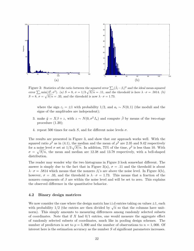
Figure 3: Statistics of the ratio between the squared error∑

i(βi−βi)2 and the ideal mean-squared

error∑

i min(β2i , σ2). (a) S = 8, σ = 1/3

√S/n = .11, and the threshold is here λ · σ = .5814. (b)

S = 8, σ =√

S/n = .33, and the threshold is now λ · σ = 1.73.

where the sign εi = ±1 with probability 1/2, and ai ∼ N(0, 1) (the moduli and thesigns of the amplitudes are independent);

3. make y = Xβ + z, with z ∼ N(0, σ2 In) and compute β by means of the two-stageprocedure (1.20);

4. repeat 500 times for each S, and for different noise levels σ.

The results are presented in Figure 3, and show that our approach works well. With thesquared ratio ρ2 as in (4.1), the median and the mean of ρ2 are 2.35 and 9.42 respectivelyfor a noise level σ set at 1/3

√S/n. In addition, 75% of the time, ρ2 is less than 10. With

σ =√

S/n, the mean and median are 12.38 and 13.78 respectively, with a bell-shapeddistribution.

The reader may wonder why the two histograms in Figure 3 look somewhat different. Theanswer is simply due to the fact that in Figure 3(a), σ = .11 and the threshold is aboutλ · σ = .5814 which means that the nonzero βi’s are above the noise level. In Figure 3(b),however, σ = .33, and the threshold is λ · σ = 1.73. This means that a fraction of thenonzero components of β are within the noise level and will be set to zero. This explainsthe observed difference in the quantitative behavior.

4.2 Binary design matrices

We now consider the case where the design matrix has i.i.d entries taking on values ±1, eachwith probability 1/2 (the entries are then divided by

√n so that the columns have unit-

norm). This simply amounts to measuring differences among randomly selected subsetsof coordinates. Note that if X had 0/1 entries, one would measure the aggregate effectof randomly selected subsets of coordinates, much like in pooling design schemes. Thenumber of predictors is set to p = 5, 000 and the number of observations to n = 1, 000. Ofinterest here is the estimation accuracy as the number S of significant parameters increases.

22

0 500 1000 1500 2000 2500 3000 3500 4000 4500 5000−4

−3

−2

−1

0

1

2

3

4

0 50 100 150 200 250 300 350 400 450 500−3

−2

−1

0

1

2

3

(a) (b)

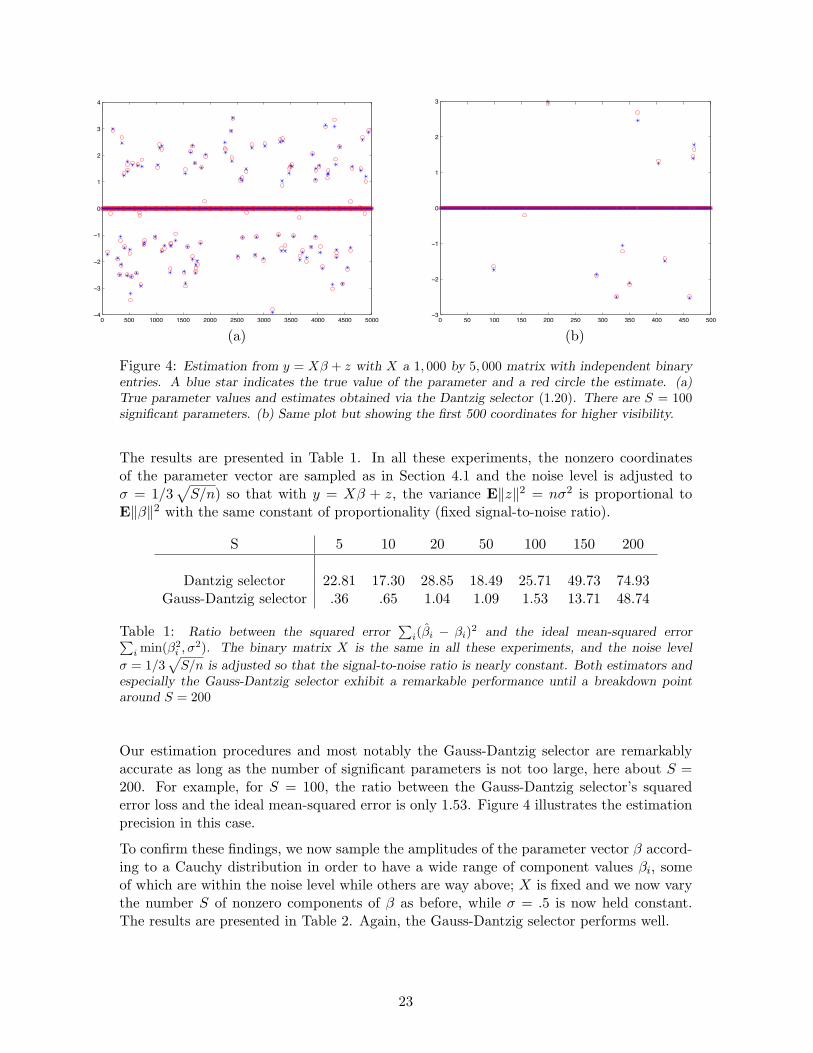
Figure 4: Estimation from y = Xβ + z with X a 1, 000 by 5, 000 matrix with independent binaryentries. A blue star indicates the true value of the parameter and a red circle the estimate. (a)True parameter values and estimates obtained via the Dantzig selector (1.20). There are S = 100significant parameters. (b) Same plot but showing the first 500 coordinates for higher visibility.

The results are presented in Table 1. In all these experiments, the nonzero coordinatesof the parameter vector are sampled as in Section 4.1 and the noise level is adjusted toσ = 1/3

√S/n) so that with y = Xβ + z, the variance E‖z‖2 = nσ2 is proportional to

E‖β‖2 with the same constant of proportionality (fixed signal-to-noise ratio).

S 5 10 20 50 100 150 200

Dantzig selector 22.81 17.30 28.85 18.49 25.71 49.73 74.93Gauss-Dantzig selector .36 .65 1.04 1.09 1.53 13.71 48.74

Table 1: Ratio between the squared error∑

i(βi − βi)2 and the ideal mean-squared error∑i min(β2

i , σ2). The binary matrix X is the same in all these experiments, and the noise level

σ = 1/3√

S/n is adjusted so that the signal-to-noise ratio is nearly constant. Both estimators andespecially the Gauss-Dantzig selector exhibit a remarkable performance until a breakdown pointaround S = 200

Our estimation procedures and most notably the Gauss-Dantzig selector are remarkablyaccurate as long as the number of significant parameters is not too large, here about S =200. For example, for S = 100, the ratio between the Gauss-Dantzig selector’s squarederror loss and the ideal mean-squared error is only 1.53. Figure 4 illustrates the estimationprecision in this case.

To confirm these findings, we now sample the amplitudes of the parameter vector β accord-ing to a Cauchy distribution in order to have a wide range of component values βi, someof which are within the noise level while others are way above; X is fixed and we now varythe number S of nonzero components of β as before, while σ = .5 is now held constant.The results are presented in Table 2. Again, the Gauss-Dantzig selector performs well.

23

S 5 10 20 50 100 150 200

Gauss-Dantzig selector 3.70 4.52 2.78 3.52 4.09 6.56 5.11

Table 2: Ratio between the squared error∑

i(βi − βi)2 and the ideal mean-squared error∑i min(β2

i , σ2). The binary matrix X, σ = .5 and λ ·σ = 2.09 are the same in all these experiments.

0 500 1000 1500 2000 2500 3000 3500 4000−40

−30

−20

−10

0

10

20

30

40

50

0 100 200 300 400 500 600−400

−300

−200

−100

0

100

200

300

400

500

600

(a) (b)

Figure 5: (a) One-dimensional signal f we wish to reconstruct. (b) First 512 wavelet coefficientsof f .

4.3 Examples in signal processing

We are interested in recovering a one-dimensional signal f ∈ Rp from noisy and undersam-pled Fourier coefficients of the form

yj = 〈f, φj〉+ zj , 1 ≤ j ≤ n,

where φj(t), t = 0, . . . , p−1 is a sinusoidal waveform φj(t) =√

2/n cos(π(kj+1/2)(t+1/2)),kj ∈ {0, 1, . . . , p − 1}. Consider the signal f in Figure 5; f is not sparse but its waveletcoefficients sequence β is. Consequently, we may just as well estimate its coefficients in anice wavelet basis. Letting Φ be the matrix with the φk’s as rows, and W be the orthogonalwavelet matrix with wavelets as columns, we have y = Xβ + z where X = ΦW , and ourestimation procedure applies as is.

The test signal is of size p = 4, 096 (Figure 5), and we sample a set of frequencies of sizen = 512 by extracting the lowest 128 frequencies and randomly selecting the others. Withthis set of observations, the goal is to study the quantitative behavior of the Gauss-Dantzigselector procedure for various noise levels. (Owing to the factor

√2/n in the definition of

φj(t), the columns of X have size about one and for each column, individual thresholds λi—|(X∗r)i| ≤ λi · σ—are determined by looking at the empirical distribution of |(X∗z)i|.) Weadjust σ so that α2 = ‖Xβ‖2/E‖z‖2 = ‖Xβ‖2/nσ2 for various levels of the signal-to-noiseratio α. We use Daubechies’ wavelets with 4 vanishing moments for the reconstruction.The results are presented in Table 3. As one can see, high statistical accuracy holds over awide range of noise levels. Interestingly, the estimator is less accurate when the noise levelis very small (α = 100) which is not surprising since in this case, there are 178 waveletcoefficients exceeding σ in absolute value.

In our last example, we consider the problem of reconstructing an image from undersampled

24

SNR α = ‖Xβ‖/√

nσ2 100 20 10 2 1 .5∑i(βi − βi)2/

∑i min(β2

i , σ2) 15.51 2.08 1.40 1.47 .91 1.00

Table 3: Performance of the Gauss-Dantzig procedure in estimating a signal from undersampledand noisy Fourier coefficients. The subset of variables is here estimated by |βi| > σ/4 with β as in(1.7). The top row is the value of the signal-to-noise ratio (SNR).

Fourier coefficients. Here β(t1, t2), 0 ≤ t1, t2 < N , is an unknown N by N image so thatp is the number of unknown pixels, p = N2. As usual, the data is given by y = Xβ + z,where

(Xβ)k =∑t1,t2

β(t1, t2) cos(2π(k1t1 + k2t2)/N), k = (k1, k2), (4.2)

or (Xβ)k =∑

t1,t2β(t1, t2) sin(2π(k1t1 + k2t2)/N). In our example (see Figure 6(b)), the

image β is not sparse but the gradient is. Therefore, to reconstruct the image, we applyour estimation strategy and minimize the `1-norm of the gradient size, also known as thetotal-variation of β

min ‖β‖TV subject to |(X∗r)i| ≤ λi · σ (4.3)

(the individual thresholds again depend on the column sizes as before); formally, the total-variation norm is of the form

‖β‖TV =∑t1,t2

√|D1β(t1, t2)|2 + |D2β(t1, t2)|2,

where D1 is the finite difference D1β = β(t1, t2) − β(t1 − 1, t2) and D2β = β(t1, t2) −β(t1, t2 − 1); in short, ‖β‖BV is the `1-norm of the size of the gradient Dβ = (D1β, D2β),see also Rudin, Osher and Fatemi (1992).

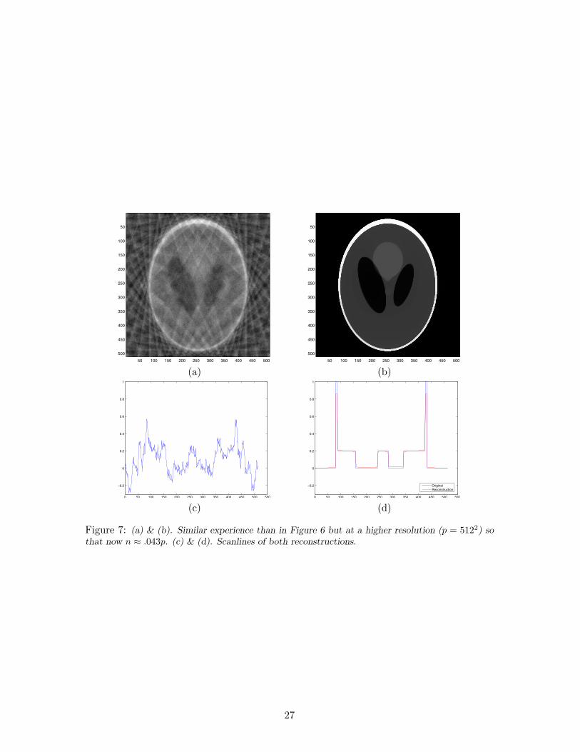
Our example follows the data acquisition patterns of many real imaging devices which cancollect high-resolution samples along radial lines at relatively few angles. Figure 6(a) il-lustrates a typical case where one gathers N = 256 samples along each of 22 radial lines.In a first experiment then, we observe 22 × 256 noisy real-valued Fourier coefficients anduse (4.3) for the recovery problem illustrated in Figure 6. The number of observations isthen n = 5, 632 whereas there are p = 65, 536 observations. In other words, about 91.5%of the 2D Fourier coefficients of β are missing. The SNR in this experiment is equal to‖Xβ‖`2/‖z‖`2 = 5.85. Figure 6(c) shows the reconstruction obtained by setting the unob-served Fourier coefficients to zero, while (d) shows the reconstruction (4.3). We follow upwith a second experiment where the unknown image is now 512 by 512 so that p = 262, 144and n = 22×512 = 11, 264. The fraction of missing Fourier coefficients is now approaching96%. The SNR ratio is about the same, ‖Xβ‖`2/‖z‖`2 = 5.77. The reconstructions are ofvery good quality, especially when compared to the naive reconstruction which minimizesthe energy of the reconstruction subject to matching the observed data. Figure 7 alsoshows the middle horizontal scanline of the phantom. As expected, we note a slight loss ofcontrast due to the nature of the estimator which here operates by “soft-thresholding” thegradient. There are, of course, ways of correcting for this bias but such issues are beyondthe scope of this paper.

25

50 100 150 200 250

50

100

150

200

250

(a) (b)

50 100 150 200 250

50

100

150

200

250

50 100 150 200 250

50

100

150

200

250

(c) (d)

0 20 40 60 80 100 120 1400

0.5

1

1.5

2

2.5

3

3.5

0 50 100 150 200 250 300−0.2

0

0.2

0.4

0.6

0.8

1

(e) (f)

Figure 6: (a) Sampling ’domain’ in the frequency plane; Fourier coefficients are sampled along22 approximately radial lines; here, n ≈ .086p. (b) The Logan-Shepp phantom test image. (c)Minimum energy reconstruction obtained by setting unobserved Fourier coefficients to zero. (d)Reconstruction obtained by minimizing the total-variation, as in (4.3). (e) Magnitude of the trueFourier coefficients along a radial line (frequency increases from left to right) on a logarithmicscale. Blue stars indicate values of log(1 + |(Xβ)k|) while the solid red line indicates the noise levellog(1 + σ). Less than a third of the frequency samples exceed the noise level. (f) X∗z and β areplotted along a scanline to convey a sense of the noise level.

26

50 100 150 200 250 300 350 400 450 500

50

100

150

200

250

300

350

400

450

500

50 100 150 200 250 300 350 400 450 500

50

100

150

200

250

300

350

400

450

500

(a) (b)

0 50 100 150 200 250 300 350 400 450 500 550

−0.2

0

0.2

0.4

0.6

0.8

1

0 50 100 150 200 250 300 350 400 450 500 550

−0.2

0

0.2

0.4

0.6

0.8

1

OriginalReconstruction

(c) (d)

Figure 7: (a) & (b). Similar experience than in Figure 6 but at a higher resolution (p = 5122) sothat now n ≈ .043p. (c) & (d). Scanlines of both reconstructions.

27

4.4 Implementation

In all the experiments above, we used a primal-dual interior point algorithm for solving thelinear program (1.9). We used a specific implementation which we outline as this gives someinsight about the computational workload of our method. For a general linear program withinequality constraints

min c∗β subject to Fβ ≤ b,

define

• f(β) = Xβ − b,

• rdual = c + X∗λ,

• rcent = −diag(λ)f(β)− 1/t,

where λ ∈ Rm are the so-called dual variables, and t is a parameter whose value typicallyincreases geometrically at each iteration; there are as many dual variables as inequalityconstraints. In a standard primal-dual method (with logarithmic barrier function) [Boydand Vandenberghe (2004)], one updates the current primal-dual pair (β, λ) by means of aNewton step, and solve(

0 F ∗

−diag(λ)F −diag(f(β))

)(∆β∆λ

)= −

(rdual

rcent

);

that is,

∆λ = −diag(1/f(β))(diag(λ)F∆β − rcent)−[F ∗diag(λ/f(β))F ]∆β = −(rdual + F ∗diag(1/f(β))rcent).

The current guess is then updated via (β+, λ+) = (β, λ) + s(∆β, ∆s) where the stepsize sis determined by line search or otherwise. Typically, the sequence of iterations stops oncethe primal-dual gap and the size of the residual vector fall below a specified tolerance level[Boyd and Vandenberghe (2004)].

Letting U = X∗X and y = X∗y in (1.9), our problem parameters have the following blockstructure

F =

I −I−I −IU 0−U 0

, b =

00

δ + yδ − y

, c =(

01

)

which gives

F ∗diag(λ/f)F =(

D1 + D2 + U∗(D3 + D4)U D2 −D1

D2 −D1 D1 + D2

),

where Di = diag(λi/fi), 1 ≤ i ≤ 4, andf1

f2

f3

f4

=

β − u

−β − u

Uβ − δ − y

−Uβ − δ + y

.

28

Put(

r1

r2

)= rdual + F ∗diag(1/f(β))rcent. It is convenient to solve the system

F ∗diag(λ/f)F(

∆β∆u

)=(

r1

r2

)by elimination and obtain

(4(D1 + D2)−1D1D2 + U∗(D3 + D4)U)∆β = r1 − (D1 + D2)−1(D1 −D2)r2

(D1 + D2)∆u = r2 − (D2 −D1)∆β.

In other words, each step may involve solving a p by p system of linear equations. Infact, when n is less than p, it is possible to solve a smaller system thanks to the Sherman-Woodbury-Morrison formula. Indeed, write U∗(D3 + D4)U = X∗B where B = X(D3 +D4)X∗X and put D12 = 4(D1 + D2)−1D1D2. Then

(D12 + X∗B)−1 = D−112 −D−1

12 X∗(I + BD−112 X∗)−1BD−1

12 .

The advantage is that one needs to solve the smaller n by n system (I + BD−112 X∗)β′ = b′.

Hence the cost of each Newton iteration is essentially that of solving an n by n system oflinear questions plus that of forming the matrix (I + BD−1

12 X∗). As far as the number ofNewton iterations is concerned, we ran thousands of experiments and have never neededmore than 45 Newton iterations for convergence.

Note that in some important applications, we may have fast algorithms for applying X andX∗ to an arbitrary vector, as in the situation where X is a partial Fourier matrix since onecan make use of FFT’s. In such settings, one never forms X∗X and uses iterative algorithmssuch as Conjugate Gradients for solving such linear systems; of course, this speeds up thecomputations.

Finally, a collection of MATLAB routines solving (1.9) for reproducing some of these ex-periments and testing these ideas in other setups is available at the following address:http://www.l1-magic.org/.

5 Discussion

5.1 Significance for Model Selection

We would like to briefly discuss the implications of this work for model selection. Given adata matrix X (with unit-normed columns) and observations y = Xβ + z, our procedurewill estimate β by that vector with minimum `1-norm among all objects β obeying

|X∗r|i ≤ (1 + t−1)√

2 log p · σ, where r = y −Xβ. (5.1)

As the theory and the numerical experiments suggest, many of the coordinates βi willtypically be zero (at least under the assumption that the true unknown vector β is sparse)and, therefore, our estimation procedure effectively returns a candidate model I := {i :βi 6= 0}.

As we have seen, the Dantzig selector is guaranteed to produce optimal results if

δ(X)2S + θ(X)S,2S < 1 (5.2)

29

(note that since θ(X)S,2S ≤ δ(X)3S , it would be sufficient to have δ(X)2S + δ(X)3S < 1).We have commented on the interpretation of this condition already. In a typical modelselection problem, X is given; it is then natural to ask if this particular X obeys (5.2) forthe assumed level S of sparsity. Unfortunately, obtaining an answer to this question mightbe computationally prohibitive as it may require checking the extremal singular values ofexponentially many submatrices.

While this may represent a limitation, two observations are in order. First, there is empir-ical evidence and theoretical analysis suggesting approximate answers for certain types ofrandom matrices, and there is nowadays a significant amount of activity developing toolsto address these questions [Daubechies (2005)]. Second, the failure of (5.2) to hold is ingeneral indicative of a structural difficulty of the problem, so that any procedure is likely tobe unsuccessful for sparsity levels in the range of the critical one. To illustrate this point,let us consider the following example. Suppose that δ2S + θS,2S > 1. Then this says thatδ2S is large and since δS is increasing in S, it may very well be that for S′ in the range ofS, e.g. S′ = 3S, there might be submatrices (in fact possibly many submatrices) with S′

columns which are either rank-deficient or which have very small singular values. In otherwords, the significant entries of the parameter vector might be arranged in such a way sothat even if one knew their location, one would not be able to estimate their values becauseof rank-deficiency. This informally suggests that the Dantzig selector breaks down near thepoint where any estimation procedure, no matter how intractable, would fail.

Finally, it is worth emphasizing the connections between RIC [Foster and George (1994)]and (1.7). Both methods suggest a penalization which is proportional to the logarithm ofthe number of explanatory variables—a penalty that is well justified theoretically [Birge andMassart (2001)]. For example, in the very special case where X is orthonormal, p = n, RICapplies a hard-thresholding rule to the vector X∗y at about O(

√2 log p), while our procedure

translates in a soft-thresholding at about the same level; in our convex formulation (1.7),this threshold level is required to make sure that the true vector is feasible. In addition,the ideas developed in this paper have a broad applicability, and it is likely that they mightbe deployed and give similar bounds for RIC variable selection. Despite such possiblesimilarities, our method differs substantially from RIC in terms of computational effortsince (1.7) is tractable while RIC is not. In fact, we are not aware of any work in the modelselection literature which is close in intent and in the results.

5.2 Connections with other works

In Candes, Romberg and Tao (2005) a related problem is studied where the goal is to recovera vector β from incomplete and contaminated measurements y = Xβ + e, where the errorvector (stochastic or deterministic) obeys ‖e‖2

`2≤ D. There, the proposed reconstruction

searches, among all objects consistent with the data y, for that with minimum `1-norm

(P2) min ‖β‖`1 subject to ‖y −Xβ‖2`2 ≤ D. (5.3)

Under essentially the same conditions as those of Theorems 1.1 and 1.2, Candes, Rombergand Tao (2005) showed that the reconstruction error is bounded by

‖β] − β‖2`2 ≤ C2

3 ·D. (5.4)

In addition, it is also argued that for arbitrary errors, the bound (5.4) is sharp and that ingeneral, one cannot hope for a better accuracy.

30

If one assumes that the error is stochastic as in this paper, however, a mean squared errorof about D might be far from optimal. Indeed, with the linear model (1.1), D ∼ σ2χn andtherefore D has size about nσ2. But suppose now β is sparse and has only three nonzerocoordinates, say, all exceeding the noise level. Then whereas Theorem 1.1 gives a loss ofabout 3σ2 (up to a log factor), (5.4) only guarantees an error of size about nσ2. What ismissing in Candes, Romberg and Tao (2005) and is achieved here is the adaptivity to theunknown level of sparsity of the object we try to recover. Note that we do not claim thatthe program (P2) is ill-suited for adaptivity. It is possible that refined arguments wouldyield estimators based on quadratically constrained `1-minimization (variations of (5.3))obeying the special adaptivity properties discussed in this paper.

Last but not least and while working on this manuscript, we became aware of relatedwork by Haupt and Nowak (2005). Motivated by recent results [Candes, Romberg andTao (2006); Candes and Tao (2004); Donoho (2004)], they studied the problem of re-constructing a signal from noisy random projections and obtained powerful quantitativeestimates which resemble ours. Their setup is different though since they exclusively workwith random design matrices, in fact random Rademacher projections, and do not studythe case of fixed X’s. In contrast, our model for X is deterministic and does not involveany kind of randomization, although our results can of course be specialized to randommatrices. But more importantly, and perhaps this is the main difference, their estimationprocedure requires solving a combinatorial problem much like (1.15) whereas we use linearprogramming.

6 Appendix

This appendix justifies the construction of a pseudo-hard thresholded vector which obeysthe constraints, see (3.17), (3.18), and (3.19) in the proof of Theorem 1.2.

Lemma 6.1 (Dual sparse reconstruction, `2 version) Let S s.t. δ+θ < 1, and let cT

be supported on T for some |T | ≤ 2S, then there exists β supported on T , and an exceptionalset E disjoint from T with

|E| ≤ S, (6.1)

such that〈Xβ, Xj〉 = cj for all j ∈ T (6.2)

and|〈Xβ, Xj〉| ≤ θ

(1− δ)√

S‖cT ‖`2 for all j 6∈ (T ∪ E) (6.3)

and(∑j∈E

|〈Xβ, Xj〉|2)1/2 ≤ θ

1− δ‖cT ‖`2 . (6.4)

Also we have‖β‖`2 ≤

11− δ

‖cT ‖`2 (6.5)

and

‖β‖`1 ≤(2S)1/2

1− δ‖cT ‖`2 (6.6)

31

Proof We define β byβT := (XT

T XT )−1cT

and zero outside of T which gives (6.2), (6.5), (6.6) by Cauchy-Schwarz. Note that Xβ =XT βT . We then set

E := {j 6∈ T : |〈Xβ, Xj〉| > θ

(1− δ)√

S‖cT ‖`2},

so (6.3) holds.

Now if T ′ is disjoint from T with |T ′| ≤ S and dT ′ is supported on T ′, then

|〈X∗T ′XT βT , dT ′〉| ≤ θ‖βT ‖`2‖dT ′‖`2

and hence by duality

‖X∗XT βT ‖`2(T ′) ≤ θ‖βT ‖`2 ≤θ

1− δ‖cT ‖`2 . (6.7)

If |E| ≥ S, then we can find T ′ ⊂ E with |T ′| = S. But then we have

‖X∗XT βT ‖`2(T ′) >θ

(1− δ)S1/2‖cT ‖`2 |T ′|1/2

which contradicts (6.7). Thus we have (6.1). Now we can apply (6.7) with T ′ := E toobtain (6.4).

Corollary 6.2 (Dual sparse reconstruction, `∞ version) Let cT be supported on Tfor some |T | ≤ S, then there exists β obeying (6.2) such that

|〈Xβ, Xj〉| ≤ θ

(1− δ − θ)√

S‖cT ‖`2 for all j 6∈ T. (6.8)

Furthermore we have‖β‖`2 ≤

11− δ − θ

‖cT ‖`2 (6.9)

and

‖β‖`1 ≤S1/2

1− δ − θ‖cT ‖`2 (6.10)

Proof The proof of this lemma operates by iterating the preceding lemma as in Lemma2.2 of Candes and Tao (2005). We simply rehearse the main ingredients and refer thereader to Candes and Tao (2005) for details.

32

We may normalize∑

j∈T |cj |2 = 1. Write T0 := T . Using Lemma 6.1, we can find a vectorβ(1) and a set T1 ⊆ {1, . . . , p} such that

T0 ∩ T1 = ∅|T1| ≤ S

〈Xβ(1), Xj〉 = cj for all j ∈ T0

|〈Xβ(1), Xj〉| ≤ θ

(1− δ)S1/2for all j 6∈ T0 ∪ T1

(∑j∈T1

|〈Xβ(1), Xj〉|2)1/2 ≤ θ

1− δ

‖β(1)‖`2 ≤1

1− δ

‖β(1)‖`1 ≤S1/2

1− δ

Applying Lemma 6.1 iteratively gives a sequence of vectors β(n+1) ∈ Rp and sets Tn+1 ⊆{1, . . . , p} for all n ≥ 1 with the properties

Tn ∩ (T0 ∪ Tn+1) = ∅|Tn+1| ≤ S

〈Xβ(n+1), Xj〉 = 〈Xβ(n), Xj〉 for all j ∈ Tn

〈Xβ(n+1), Xj〉 = 0 for all j ∈ T0

|〈Xβ(n+1), Xj〉| ≤ θ

(1− δ)S1/2

(θ

1− δ

)n

∀j 6∈ T0 ∪ Tn ∪ Tn+1

(∑

j∈Tn+1

|〈Xβ(n+1), Xj〉|2)1/2 ≤ θ

1− δ

(θ

1− δ

)n

‖β(n+1)‖`2 ≤1

1− δ

(θ

1− δ

)n−1

‖β(n+1)‖`1 ≤S1/2

1− δ

(θ

1− δ

)n−1

.

By hypothesis, we have θ1−δ ≤ 1. Thus if we set

β :=∞∑

n=1

(−1)n−1β(n)

then the series is absolutely convergent and, therefore, β is a well-defined vector. And itturns out that β obeys the desired properties, see Lemma 2.2 in Candes and Tao (2005).

Corollary 6.3 (Constrained thresholding) Let β be S-sparse such that

‖β‖`2 < λ · S1/2

33

for some λ > 0. Then there exists a decomposition β = β′ + β′′ such that

‖β′‖`2 ≤1 + δ

1− δ − θ‖β‖`2

and

‖β′‖`1 ≤1 + δ

1− δ − θ

‖β‖2`2

λ

and

‖X∗Xβ′′‖`∞ <1− δ2

1− δ − θλ.

Proof LetT := {j : |〈Xβ, Xj〉| ≥ (1 + δ)λ}.

Suppose that |T | ≥ S, then we can find a subset T ′ of T with |T ′| = S. Then by restrictedisometry we have

(1 + δ)2λ2S ≤∑j∈T ′

|〈Xβ, Xj〉|2 ≤ (1 + δ)‖Xβ‖2`2 ≤ (1 + δ)2‖β‖2

`2 ,

contradicting the hypothesis. Thus |T | < S. Applying restricted isometry again, we con-clude

(1 + δ)2λ2|T | ≤∑j∈T

|〈Xβ, Xj〉|2 ≤ (1 + δ)2‖β‖2`2

and hence

|T | ≤ S :=‖β‖2

`2

λ2.

Applying Corollary 6.2 with cj := 〈Xβ, Xj〉, we can find an β′ such that

〈Xβ′, Xj〉 = 〈Xβ, Xj〉 for all j ∈ T

and‖β′‖`2 ≤

1 + δ

1− δ − θ‖β‖`2

and

‖β′‖`1 ≤(1 + δ)

√S

1− δ − θ‖β‖`2 =

(1 + δ)1− δ − θ

‖β‖2`2

λ

and|〈Xβ′, Xj〉| ≤ θ(1 + δ)

(1− δ − θ)√

S‖β‖`2 for all j 6∈ T.

By definition of S we thus have

|〈Xβ′, Xj〉| ≤ θ

1− δ − θ(1 + δ)λ for all j 6∈ T.

Meanwhile, by definition of T we have

|〈Xβ, Xj〉| < (1 + δ)λ for all j 6∈ T.

Setting β′′ := β − β′, the claims follow.

34

References

Akaike, H. (1974). A new look at the statistical model identification. IEEE Trans. AutomaticControl 19 716–723.

Antoniadis, A. and Fan, J. (2001). Regularization of wavelet approximations. With discus-sion and a rejoinder by the authors. J. Amer. Statist. Assoc. 96 939–967.

Baraud, Y. (2000). Model selection for regression on a fixed design. Probab. Theory RelatedFields 117 467–493.

Barron, A. R., Birge, L. and Massart, P. (1999). Risk bounds for model selection viapenalization. Probab. Theory Related Fields 113 301–413.

Barron, A. R. and Cover, T. M. (1991). Minimum complexity density estimation. IEEETrans. Inform. Theory 37 1034–1054.

Birge, L. and Massart, P. (1997). From model selection to adaptive estimation. In Festschriftfor Lucien Le Cam 55–87. Springer, New York.

Birge, L. and Massart, P. (2001). Gaussian model selection. J. Eur. Math. Soc. (JEMS) 3203–268.

Boyd, S. and Vandenberghe L. (2004). Convex Optimization. Cambridge University Press.

Candes, E. J., Romberg, J. and Tao, T. (2006). Robust uncertainty principles: exact sig-nal reconstruction from highly incomplete frequency information. IEEE Trans. Inform.Theory 52 489-509.

Candes, E. J. and Tao, T. (2004). Near optimal signal recovery from random projections:universal encoding strategies? To appear in IEEE Trans. Inform. Theory. Available onthe ArXiV preprint server: math.CA/0410542.

Candes, E. J. and Tao, T. (2005). Decoding by linear programming. IEEE Trans. Inform.Theory 51 4203-4215.

Candes, E. J. and Romberg, J. (2005). Practical signal recovery from random projections.In SPIE International Symposium on Electronic Imaging: Computational Imaging IIISan Jose, California.

Candes, E. J., Romberg, J. and Tao, T. (2005). Stable signal recovery from incomplete andinaccurate measurements. Comm. Pure Appl. Math. (in press). Available on the ArXiVpreprint server: math.NA/0503066.

Candes, E. J., Rudelson, M., Vershynin, R. and Tao, T. (2005). Error Correction via linearprogramming. In Proceedings of the 46th Annual IEEE Symposium on Foundations ofComputer Science (FOCS) 295–308.

Chen, S. S., Donoho, D. L. and Saunders, M. A. (1999). Atomic decomposition by basispursuit. SIAM J. Scientific Computing 20 33–61.

Daniel, B. L., Yen, Y. F. and Glover, G. H. (1998). Breast disease: dynamic spiral MRimaging. Radiology 209 499–509.

35

Daubechies, I. (2005). Personal communication.

Donoho, D. L. and Johnstone, I. M. (1994a). Ideal spatial adaptation by wavelet shrinkage.Biometrika 81 425–455.

Donoho, D. L. and Johnstone, I. M. (1994b). Ideal denoising in an orthonormal basis chosenfrom a library of bases. C. R. Acad. Sci. Paris Ser. I Math. 319 1317–1322.

Donoho, D. L. and Johnstone, I. M. (1995). Empirical atomic decomposition. Unpublishedmanuscript.

Donoho, D. L. and Huo, X (2001). Uncertainty principles and ideal atomic decomposition.IEEE Trans. Inform. Theory 47 2845–2862.

Donoho, D. L. (2004). For Most Large Underdetermined Systems of Linear Equations theMinimal `1-norm Solution is also the Sparsest Solution. Manuscript.

Donoho, D. L (2004). Compressed sensing. Manuscript.

Elad, M. and Bruckstein, A. M. (2002). A generalized uncertainty principle and sparserepresentation in pairs of bases. IEEE Trans. Inform. Theory 48 2558–2567.

Fan, J. and Peng, H. (2004). Nonconcave penalized likelihood with a diverging number ofparameters. Ann. Statist. 32 928–961.

Foster, D. P. and George, E. I. (1994). The risk inflation criterion for multiple regression.Ann. Statist. 22 1947–1975.

Fuchs, J. (2004). On sparse representations in arbitrary redundant bases. IEEE Trans.Inform. Theory 50 1341–1344.

Greenshtein, E. and Ritov, Y. (2004). Persistence in high-dimensional linear predictor se-lection and the virtue of overparametrization. Bernoulli 10 971–988.

Haupt, J. and Nowak, R. (2005). Signal reconstruction from noisy random projections.Submitted to IEEE Trans. Info. Theory.

Statistics: Challenges and Opportunities for the Twenty-First Century. NSF report. Editedby: Jon Kettenring, Bruce Lindsay, and David Siegmund, April 2003.

Mallows, C. L. (1973). Some comments on Cp. Technometrics 15 661–676.

Natarajan, B. K. (1995). Sparse approximate solutions to linear systems. SIAM J. Comput.24 227-234.

Peters, D. C., Grist, T. M., Korosec, F. R., Holden, J. E., Block, W. F., Wedding, K.L., Carroll, T. J. and Mistretta, C. A. (2000). Undersampled projection reconstructionapplied to MR angiography. Magn. Reson. Med. 43 91–101.

Rudin, L. I., Osher, S. and Fatemi, E. (1992). Nonlinear total variation noise removalalgorithm. Physica D 60 259–268.

Sardy, S., Bruce, A. G. and Tseng, P. (2000). Block coordinate relaxation methods fornonparametric wavelet denoising. J. Comput. Graph. Statist. 9 361–379.

36

Schwarz, G. (1978). Estimating the dimension of a model. Ann. Statist. 6 461–464.

Szarek, S. J. (1991). Condition numbers of random matrices. J. Complexity 7 131–149.

Tibshirani, R. (1996). Regression shrinkage and selection via the lasso. J. Roy. Statist. Soc.Ser. B 58 267–288.

37