Working Paper 25637http://www.nber.org/papers/w25637
NATIONAL BUREAU OF ECONOMIC RESEARCH1050 Massachusetts Avenue
Cambridge, MA 02138March 2019
We are indebted to Ryan Johnson and Erik Daubert from the YMCA of the USA for their invaluable guidance and expertise in setting up our research partnership, as well as to Maria-Alicia Serrano for her continuing support. We wish to thank the YMCA of the Triangle Area, particularly Tony Campione, Mark Julian, Brian Spanner, and Janet Sprague, for their outstanding support in implementing our field experiments. We are grateful to Leonardo Bursztyn, Gary Charness, Alain Cohn, Jonathan Davis, Stefano DellaVigna, Ray Fisman, Jana Gallus, David Gill, Alex Imas, John List, Keith Ericson, Fatemeh Momeni, Ricardo Perez-Truglia, Daniel Tannenbaum, as well as numerous conference and seminar participants for helpful comments. The views expressed herein do not necessarily reflect the views of the YMCA of the USA or any other YMCA member association. The experiment was approved by University of Chicago IRB, #IRB15-1647. The views expressed herein are those of the authors and do not necessarily reflect the views of the National Bureau of Economic Research.
NBER working papers are circulated for discussion and comment purposes. They have not been peer-reviewed or been subject to the review by the NBER Board of Directors that accompanies official NBER publications.
The Deadweight Loss of Social RecognitionLuigi Butera, Robert Metcalfe, William Morrison, and Dmitry TaubinskyNBER Working Paper No. 25637March 2019JEL No. D8,D9,H0,I0
ABSTRACT
A growing body of empirical work shows that social recognition of individuals' behavior can meaningfully influence individuals’ choices. This paper studies whether social recognition is a socially efficient lever for influencing individuals’ choices. Because social recognition generates utility from esteem to some but disutility from shame to others, it can be either positive-sum, zero-sum, or negative-sum. This depends on whether the social recognition utility function is convex, linear, or concave, respectively. We develop a new revealed preferences methodology to investigate this question, which we deploy in a field experiment on promoting attendance to the YMCA of the Triangle Area. We find that social recognition increases YMCA attendance by 17-23% over a one-month period in our experiment, and our estimated structural models predict that it would increase attendance by 19-23% if it were applied to the whole YMCA of the Triangle Area population. However, we find that the social recognition utility function is significantly concave and thus generates deadweight loss. If our social recognition intervention were applied to the whole YMCA of the Triangle Area population, we estimate that it would generate deadweight loss of $1.23-$2.15 per dollar of behaviorally-equivalent financial incentives.
Luigi ButeraDepartment of Economics Copenhagen Business School [email protected]
William MorrisonUniversity of California, Berkeley530 Evans HallMC #3880Berkeley, CA 94720 [email protected]
Dmitry TaubinskyUniversity of California, Berkeley Department of Economics530 Evans Hall #3880Berkeley, CA 94720-3880and [email protected]
1 Introduction
The human desire for social recognition is a powerful motivator. Many organizations around the
world leverage this to affect a variety of economically important behaviors (Loewenstein et al., 2014;
Bursztyn and Jensen, 2017). For instance, 89% of businesses use some form of social recognition
programs (WorldatWork, 2017), including examples like “employee of the month” (Kosfeld and
Neckermann, 2011). Bloom and Van Reenen (2007) find that 60% of manufacturing companies
publicly reveal and compare employees’ performance data. Governments also use social recognition
programs to motivate citizens to pay their taxes (Bø et al., 2015; Perez-Truglia and Troiano, 2018),
to motivate bureaucrats to do a better job (Gauri et al., 2018), and to encourage teachers, doctors,
and managers in schools and hospitals to improve their performance. Charities often utilize social
recognition in the form of giving circles (Karlan and McConnell, 2014).
Recent field experiments confirm that public recognition of individuals’ behavior does, indeed,
have substantial effects on behavior in a number of economically important domains. Examples
include increasing charitable and political donations (Perez-Truglia and Cruces, 2017) by recog-
nizing the donors; increasing tax compliance by publicizing it to neighbors (Perez-Truglia and
Troiano, 2018); affecting education and career choices by manipulating the observability to one’s
peers (Bursztyn and Jensen, 2015; Bursztyn et al., 2017b, 2019); increasing employee productivity
by publicizing ranks (Barankay, 2011; Ashraf et al., 2014; Bradler et al., 2016); increasing voter
turnout by publicizing voting records to neighbors (Gerber et al., 2008); increasing childhood immu-
nization by publicizing progress through the bracelets given to children (Karing, 2019); increasing
the sign up rates for energy conservation programs (Yoeli et al., 2013); and increasing the take-up
of credit cards by making them a status signal (Bursztyn et al., 2017a).
Yet social recognition is an emblematic example of why it is crucial to carefully quantify the
costs and benefits generated by non-financial levers. It is a positional good: not everyone can be
at the top, and so greater visibility brings esteems to some but shame to others. The total sum
of the gains from esteem and the losses from shame determines the economic efficiency of utilizing
social recognition to affect behavior.
In this paper, we develop a novel approach to analyzing the welfare effects of changing behavior
using social recognition. Although it is often assumed that one’s social recognition utility is linear in
the audience’s inferences about one’s type (e.g., Benabou and Tirole 2006, 2011; Ali and Benabou
2016), we show that this assumption is far from innocuous for questions about the efficiency of
social recognition interventions. Deviations from linearity can generate deadweight loss from social
recognition—the extent to which surplus would be higher if behavior change was instead achieved
by revenue-neutral financial incentives. Any intervention that leverages social recognition—whether
fully or partially revealing—will generate deadweight loss if the social recognition utility function
is concave. This result is a consequence of Jensen’s inequality. Intuitively, the gains from esteem
for the above-average types will be less intense than the losses from shame for the below-average
types. Conversely, the intervention will generate additional social surplus if the social recognition
utility function is convex.
1
We then develop a revealed preferences methodology for estimating the curvature of the social
recognition utility function. We do this by eliciting people’s (possibly negative) willingness to pay
for social recognition conditional on different possible realized future behaviors. This method is
robust to forecasting biases that would otherwise invalidate a revealed preferences welfare analysis
of non-price levers such as ours.
We implement our approach in a field experiment conducted in partnership with the YMCA of
the USA1 and the YMCA of the Triangle Area (YOTA) in Raleigh, North Carolina.2 We invited
all members of YOTA to participate in a newly designed one-month program called “Grow &
Thrive”. This program encouraged members to attend their local YMCA more often by having
an anonymous donor give $2 to the local YMCA for each day that an individual attended the
YMCA. Participants could also be randomly assigned to an additional treatment group, the “social
recognition program,” (SRP) which would reveal each participant’s attendance and donations raised
to all other participants in SRP.
To directly estimate a money-metric measure of consumer surplus from social recognition, we
elicited willingness to pay (WTP) for social recognition as follows: Prior to the start of the month-
long period during which incentives for attendance were provided, participants in our experiment
were asked to provide their WTP (possibly negative) for being in the social recognition group,
for each possible realization of their attendances during Grow & Thrive. To make this incentive
compatible, WTP was elicited using the Becker-DeGroot-Marschak (BDM) mechanism.3 But to
generate random assignment, as well as to minimize any negative inferences that could be drawn
about participants who are not in the social recognition group, we guaranteed that the BDM
responses would be used to determine assignment only with 10% chance. With 90% chance par-
ticipants would be randomly assigned to be in the social recognition group or not, independent
of their BDM decisions. This information was common knowledge among participants. Prior to
making their WTP decisions, individuals were also informed about the average YOTA attendance
in the prior month.
Our findings are threefold. First, we document that social recognition increases YMCA atten-
dance by approximately 17-23% during the treatment month. This percent increase is roughly the
same for individuals with low and high prior attendance.
Second, we provide a direct, non-parametric quantification of social recognition utility, and
confirm the key monotonicity assumption of all models of social recognition. We find that indi-
viduals’ WTP for social recognition, conditional on the number of times they might attend the
YMCA during Grow & Thrive, is strictly increasing in this potential future attendance: it ranges
from a -$1.70 for zero attendances to $2.61 for twenty-three or more attendances. Perhaps most
1The YMCA of the USA is a national, non-profit, charitable organization that supports local communities witha focus on youth development, healthy living, and social responsibility. Please see http://www.ymca.net/.
2One of the 850 member association YMCAs, YMCA of the Triangle Area primarily serves the Raleigh-Durham,North Carolina and surrounding communities.
3As we argue in Section 3, WTP in this mechanism directly reflects the (forecasted) hedonic effects of socialrecognition, and is not affected by preferences for commitment if there are time-inconsistent individuals in thepopulation.
2
importantly, these data directly reveal that social recognition produces both winners and losers.
This finding of both winners and losers sets up our core question: is social recognition positive-
sum, zero-sum, or negative-sum? To answer this question, we begin by documenting significant
concavity in our non-parametric elicitation of social recognition utility. This implies that social
recognition is negative-sum both in “action-based” models in which individuals care about how
their action compares to the average (e.g., Becker, 1991; Besley and Coate, 1992; Blomquist, 1993;
Lindbeck et al., 1999), and in “type-based” models in which individuals care about what their
action reveals about their “type” (e.g., Benabou and Tirole, 2006; Andreoni and Bernheim, 2009;
Ali and Benabou, 2016).
We then build on this qualitative finding by estimating structural models of social recognition
utility. These structural models allow us to quantify the behavior change and deadweight loss that
would be generated if our social recognition intervention were applied broadly to all members of the
YMCA of the Triangle Area. Performing such an exercise requires characterizing the equilibria of
our models to take into account the fact that such an intervention would shift the equilibrium, and
thus the social recognition payoffs tied to any one action. For example, individuals who evaluate
their behavior relative to the average would have a more demanding average to compare to, since a
broadly applied social recognition intervention would increase everyone’s attendance. We estimate
that a social recognition intervention would change behavior by additional 0.60-0.72 attendances
per month, a change that could be equivalently produced by financial incentives of $0.27-$0.36 per
attendance. However, this change in behavior generates $0.32-0.35 of deadweight loss, or $1.23-
$2.15 per dollar of behaviorally-equivalent financial incentives.
The finding of significant deadweight loss not only generates considerations for policy, but also
for the efficiency of the social recognition incentives used by employers and other interested organi-
zations. In our setting, individuals are significantly over-optimistic about their future attendance,
which would lead them to overvalue the benefits of being in an environment in which their atten-
dance is socially recognized. In the last part of the paper we argue that markets may over-use
social recognition incentives in lieu of financial incentives if individuals mis-forecast their future
performance.
As we emphasize in the concluding section, our contributions are methodological as much they
are substantive. We end by discussing a number of reasons for why caution should be taken in
extrapolating too strongly from our specific results. But we hope that in future work, researchers
can utilize or build on our methods to analyze not only the effects of social recognition on behavior,
but also on social surplus.
Our research is related to several literatures. The most closely related is the large and growing
field experimental literature studying the effects of social recognition on individual behavior. How-
ever, this literature does not ask whether social recognition is a socially efficient means of bringing
about that behavior change. We build on this literature by setting it in a generally applicable
welfare framework that extends the central economic concept of deadweight loss.
Our work also relates to a recent literature that evaluates the welfare effects of scalable, “nudge-
3
style” non-price interventions such as reminders (Damgaard and Gravert, 2018), energy-use social
comparisons (Allcott and Kessler, 2019), calorie labeling (Thunstrom, 2019), and defaults (Carroll
et al., 2009; Bernheim et al., 2015). Beyond analyzing a different and highly popular non-price
intervention, we add several technical innovations to this important literature. First, while these
papers study the impact of the intervention on consumer surplus only, we extend the concept of
deadweight loss to study how socially efficient the intervention is in bringing about the desired
behavior change. The focus on deadweight loss makes it possible to consider the efficiency rankings
of an arsenal of different possible policy levers, and to have a direct comparison to standard financial
incentives. As a simple analogy, while other papers can be seen as evaluating, e.g., the welfare effects
of fuel economy standards, our paper provides a framework for asking whether carbon emissions
are most efficiently reduced through fuel economy standards or Pigovian taxation or some other
policy.
Second, our field experiment utilizes a new design technique, grounded in “strategy method”
approaches typically only used in laboratory experiments, that eliminates the need to rely on the
assumption that individuals can correctly forecast their future behavior.4 We establish the need to
relax this assumption in our setting, and we discuss its relevance for other studies.
Finally, our model-based design allows us to produce the first structural estimates of leading
models of social recognition such as those of Benabou and Tirole (2006).5 We therefore also
contribute to a recent and growing literature in structural behavioral economics (see DellaVigna,
2018 for a review). The work by DellaVigna et al. (2012) and DellaVigna et al. (2017) is closest
in spirit to our paper in this literature, although they do not study the scalable lever of revealing
peoples’ behavior to others, nor do they estimate the leading social recognition models. These
two papers quantify the cost of social pressure exerted by a solicitor to donate, and of the social
pressure to tell a get-out-the-vote surveyor that one has voted, respectively.6 They do this by using
structural methods to infer the cost of social pressure from the degree to which individuals avoid
interaction with others. In contrast, we use conceptually different, and more direct experimental
techniques that leverage the richness of our action space and allow us to directly observe the shape
of utility from the social motives. We also develop structural estimation methods for making out-
of-sample predictions that take into account that the effects of a non-price lever may change in
4See also Bernheim and Taubinsky (2018) for a more detailed discussion of the weaknesses of this assumption, aswell as the “non-comparability problem” that less theory-grounded approaches such as those of Allcott and Kessler(2019) are subject to.
5Karing (2019), Bursztyn et al. (2019), Ariely et al. (2009), and Exley (2018) test comparative statics of theBenabou and Tirole (2006) model, and Karing (2019) quantifies the value of sending a positive (but not fully-revealing) signal. These papers do not estimate the underlying social recognition utility function.
6We delineate between social pressure and social recognition. Social pressure commonly refers to situations inwhich individuals take actions as a response to direct peers’ influence or requests; an example is DellaVigna et al.(2012), where the social pressure is a force layered on top of the information already revealed by choosing to use ado-not-visit tag. Social recognition instead refers to situations in which individuals take actions to influence others’beliefs about them. In some settings both are in play; e.g., when telling a surveyor whether or not one has voted, asin DellaVigna et al. (2017). The implicit assumption of the DellaVigna et al. (2017) model that not answering thedoor to a pre-announced visit (an action most likely to be taken by those who did not vote) generates no disutilitybeyond hassle costs is more consistent with a social pressure interpretation and less consistent with leading socialsignaling models such as those of Benabou and Tirole (2006) and Andreoni and Bernheim (2009).
4
equilibrium. We do this by formally working out the (somewhat different) equilibrium predictions
of the microfounded models that we estimate.
The remainder of the paper is organized as follows. Section 2 introduces our theoretical frame-
work and provides our definitions of deadweight loss. Section 3 lays out our experimental design.
Section 4 reports the reduced-form results from our experiment. Section 5 presents our estimates of
the structural models, and the deadweight loss that they imply. Section 7 concludes by discussing
limitations, robustness, and questions for future research.
2 Conceptual framework for analysis
In this section we begin by describing two models of preferences over social recognition. In the
first model, individuals care about how their observed performance compares to the average per-
formance. In the second model, individuals care about what the audience infers to be their “type.”
After presenting the models, we formally define the deadweight loss of social recognition that arise
from both models. We conclude by discussing the challenges of estimating these models using
experimental data.
2.1 The models
We consider individuals who choose the level of intensity a ∈ A ⊂ R+ to engage in some activity.
Choosing a generates material utility u(a; θ) + y, where y is the individual’s income and θ is the
type of the individual, distributed according to some atomless distribution F over R. Assuming
that utility is linear in income is a simplifying assumption that is not crucial for our theoretical
exposition, but that is realistic given the relatively small financial stakes of our experimental setting.
We assume that u(a; θ) is single-peaked in a and that ddau(a; θ) is increasing in θ and is bounded.
In words, each individual has some optimal intensity level a∗(θ), and higher types derive more
benefit from choosing higher levels of a. In addition to material utility, individuals also derive
social recognition utility S, which we define below.
2.1.1 Action-based social recognition
The first model that we consider posits that when an individual’s action is made public, the
individual cares about how his action compares to the average action of the population (Becker,
1991; Besley and Coate, 1992; Blomquist, 1993; Lindbeck et al., 1999, 2003). Formally, utility is
u(a; θ) + y + νS(a− a),
where ν is the visibility parameter, a is the average action in the population, and S is increasing
and satisfies S(0) = 0. The model captures the simple intuition that individuals derive “pride”
5
from doing better than the average, and “shame” from doing less well than the average.7 We follow
Ali and Benabou (2016) in defining the visibility parameter ν to capture the degree of visibility,
such as the number of observers. Reference points other than the average behavior a are possible
(e.g., the median); but as we shall show, the reference point of average behavior matches our results
well.
2.1.2 Type-based social recognition
The second model posits that individuals derive utility from what their action reveals about their
type to the audience (e.g., Andreoni and Bernheim, 2009; Benabou and Tirole, 2006; Ali and
Benabou, 2016). Formally, utility is
u(a; θ) + y + νS(E[θ|a]; θ)
where ν is the visibility parameter, E[θ|a] is the audience’s inference about θ given observed action
a, θ is the average type in the population, and S is increasing in E[θ|a] and satisfies S(θ, θ) = 0.
The last assumption that S(θ, θ) = 0 simply says that no matter how large the audience, if no
information is revealed about a person’s type then the utility from social recognition is zero. Our
formulation is identical to that of Ali and Benabou (2016), with the single but crucial difference
that we do not assume that S is linear.
2.2 The deadweight loss of social recognition
In both models, individuals who are recognized as being below average incur utility losses, while
individuals who are recognized as above average enjoy utility gains. Whether social recognition
is positive-sum, zero-sum, or negative-sum in either model depends on the curvature of the so-
cial recognition utility function S. For example, if S is (strictly) concave, and if Eθ denotes the
expectation with respect to types θ who choose actions a(θ), then Jensen’s Inequality implies
in the type-based model. That is, concavity of S makes social recognition negative-sum. Conversely,
identical arguments show that convexity of S makes social recognition positive-sum, and linearity
7Although this class of models is typically formulated for deterministic economic environments such as ours,in which actions are perfectly observed, the model is easily extended to allow for imperfect observability. Givenaudiences beliefs H(·|s) about the action a given some signal σ about the action, expected social recognition utilitycan be defined as
∫S(a− a)dH(a|σ).
8In a more general version of this model in which actions may be imperfectly observed, defined in footnote 7,the average payoffs from social recognition are similarly given by Eθ[E[S(a − a)|σ(θ)]] < S(Eθ[E[a(θ) − a|σ(θ)]]) =S(0) = 0.
6
makes it zero-sum.9 Despite its strong implications for social welfare, linearity is a commonly
made assumption in papers that study the broader policy implications of social recognition, such
as Benabou and Tirole (2011), Ali and Benabou (2016) and others.
These implications of curvature hold for any kind of public recognition scheme, not just one
that reveals individuals’ actions perfectly. This includes, for example, two-tier social recognition
schemes that publicize only the behavior of the top performers. In the type-based model, suppose
that instead of observing an action, the audience observes some signal σ about a person’s type
(which can be affected by the actions undertaken). Replacing a(θ) with σ(θ) in equation (2)
generates the identical inequality. The same holds for the action-based model, as worked out in
footnote 8. Intuitively, this is because not being recognized as a top performer is a signal about
one’s actions and type. Those individuals would prefer to be seen as “average” among everyone,
rather than “average” among all but the top.
Intuitively, the question we seek to answer is the extent to which social recognition is positive-
sum, zero-sum, or negative-sum; that is, what is the value of E[S]? We formalize this by extending
the economic concept of deadweight loss to apply to social recognition. Recall that the deadweight
loss of a distortionary tax is the amount by which consumer surplus would be higher if the same tax
revenue were instead raised through a lump-sum tax instead; that is, it is the impact on consumer
surplus relative to the benchmark of a lump-sum transfer. To define the deadweight loss of social
recognition, the benchmark we adopt is revenue-neutral financial incentives that achieve the same
change in behavior—for each type θ—that social recognition does.
Definition 1. The deadweight loss of social recognition is the amount by which consumer surplus
would be higher if the same behavior (by type) change were instead produced by revenue-neutral
financial incentives.
Appendix A provides a formal definition of deadweight loss that follows the deadweight loss
of taxation definition in Auerbach (1985), and that is applicable to utility functions that are not
quasilinear in income. But for the quasilinear case, the deadweight loss definition is equivalent to
simply taking the average of the realized values of S in the population. An immediate implication
of equations (1) and (2), therefore, is that when S is concave, social recognition produces positive
deadweight loss. Conversely, when S is convex, social recognition produces negative deadweight
loss; i.e., social surplus. Finally, when S is linear, social recognition produces zero deadweight loss.
Quantitatively, these effects are magnified by higher visibility ν. These effects may also be
affected by nature of the social recognition scheme: publicizing everyone’s behavior rather than
just those of the top performers will lead to both different effects on behavior and to different
deadweight loss estimates (but will not change the sign of the deadweight loss estimates, as we
argued above).
These considerations imply that the deadweight loss statistic in Definition 1 does not make clear
9There is also a possibility that the curvature of S changes signs as the attendance changes. For example, wecould in theory have a convex S for θ < θ and concave S for θ ≥ θ. We show in Section 4.3 that the reduced form Sin our setting is well approximated by a quadratic function with global curvature.
7
in a general sense how inefficient (or efficient) social recognition is relative to financial incentive
schemes. In particular, note that both deadweight loss and the change in behavior are increasing
in ν, and thus deadweight loss might be small either because the visibility is low or because S
exhibits little curvature. It is thus more appropriate to consider a normalized, unitless measure of
deadweight loss, that is not tied directly to ν.
To do so, we define pν(θ) to be the linear piece-rate incentive that would have to be given to
each type θ to induce the same change in behavior as the change created by increasing visibility
from 0 to ν. We call pν = Epν(θ) the equivalent price metric (EPM) of the social recognition
intervention.10 We use this to construct the following unitless measure:
Definition 2. The deadweight loss per dollar of behaviorally-equivalent financial incentives is the
deadweight loss per unit change in behavior, divided by the equivalent price metric.
Note that simply dividing deadweight loss by its total impact on behavior generates a measure
that is in units of dollars per unit of action, and is thus inconveniently tied to the units in which
behavior change is measured. Direct comparisons of deadweight loss across different contexts would
thus not be possible with such a measure. The unitless measure in Definition 2, however, enables
such direct comparisons.
As with the analysis of the deadweight loss of taxation, we separate the question of deadweight
loss from questions about the aggregate benefits of the policy. In the same way that questions
about deadweight loss of taxation do not touch on how the tax revenue will be used, questions about
deadweight loss of social recognition do not touch on the benefits of behavior change itself. Instead,
our question is about the efficacy of social recognition, compared to to standard financial incentives,
in producing the desired behavior change. Just as fuel economy standards can improve social welfare
but are second-best to Pigouvian taxes, social recognition has the capacity to increase welfare while
simultaneously creating deadweight loss relative to behaviorally-equivalent financial incentives. The
goal of the deadweight loss concept is to facilitate such economic efficiency comparisons.
2.3 Measuring deadweight loss using experiments
Often, the economic questions of interest are about the effects of utilizing social recognition on a
whole population, not just the experimental sample. Answering this question requires an additional
step of analysis, because the equilibrium response of an individual in an experiment can be very
different from equilibrium response of that same individual when social recognition is scaled up to
the broader population.
To formalize, call R : A → R the reduced-form social recognition function which assigns, for
each value a, a social recognition payoff. Let Rexp denote the function elicited for the experimental
population during the experiment, and let Rpop denote the reduced-form social recognition function
that would result if social recognition was applied to the whole population of interest. These two
10For types θ who do not change their behavior because their optimal choice of action is at a corner, pν(θ) isundefined. The average pν averages only over types for which the pν is defined.
8
objects can be meaningfully different: when the social recognition lever is applied to the whole
population, population behavior changes, and thus the benchmark for what is considered relatively
good behavior changes as well.
As a simple example, suppose that in our YMCA setting, an individual is observed to have
attended the YMCA four times during the month of the experiment, and that average population
attendance is 3.5 attendances. In the context of the experiment, an individual attending four times
would thus receive positive social recognition payoffs under the action-based social recognition
model. However, suppose that after applying the social recognition intervention to the whole
population, average attendance would increase to 4.5 attendances. Then an attendance of four
would actually generate negative social recognition utility.
Building on this insight, it is apparent that even if the experimental population was perfectly
representative of the full population, average social recognition utility could be positive in the
experiment, despite S being concave and social recognition being negative-sum in reality. Thus,
the inference based on Rexp might generate misleading conclusions about deadweight loss.
An important element of our analysis will be to utilize microfounded models of social recognition
to extrapolate S from Rexp, and consequently to obtain Rpop. Our reading of existing literature
studying social comparisons and social pressure is that it stops at Rexp.11
The questions about equilibrium responses are separable from other concerns about external
validity, such as the possible non-representativeness of the experimental sample. For example, in
our experiment we do not find any interaction between social recognition utility and observable
characteristics, but we cannot rule out selection on unobservables that are correlated with social
recognition utility functions. These other questions about external validity (for a review, see Duflo
et al., 2007; Al-Ubaydli et al., 2017; Banerjee et al., 2017; Davis et al., 2017) are important questions
for assessing any kind of field experiment. Our point about equilibrium, however, is intrinsically
connected to the formal microfoundations of the intervention being tested. While signaling models
are, intrinsically, equilibrium models, there are many “nudge-style” interventions, such as salient
information disclosure, where the treatment effects are not determined in equilibrium.
11For example, suppose that individuals’ utility in the Allcott and Kessler (2019) is a decreasing function of thedifference between their energy use and the energy use of the neighbors they are shown. Then the utility that theyreceive from the information mailer depends on whether the mailer goes out to their neighbors as well. However,since not everyone received the mailer in the experiment, the reduced-form effects that they estimate cannot beused to directly evaluate the policy of sending out mailers to all households. To perform such an evaluation, itwould be necessary to take a stand on the structural utility function for social comparisons, to estimate it usingthe experimental results, and to estimate the counterfactual equilibrium of sending the mailers to everyone in thepopulation.
As another example, consider evaluating individuals’ utility from encountering a surveyor who asks about votingbehavior. DellaVigna et al. (2017) estimate the utility of doing so after the votes have already been cast. But toevaluate the equilibrium impact of increasing the visibility of one’s voting behavior, it is necessary to account forthe fact that visibility also changes voting behavior, which changes the payoffs one receives from telling a surveyorif one has voted or not. Evaluating the equilibrium outcomes would thus require one to estimate the structuralmicrofoundations of why individuals like to tell others that they voted.
9
3 Experimental design
3.1 Overview
The field experiment was conducted in collaboration with the YMCA of USA and the YMCA of the
Triangle Area in North Carolina (YOTA), and was publicly called “Grow & Thrive”. YMCA mem-
bers of two large YMCA facilities from YOTA were invited via email to sign up to this program by
completing a survey. They were informed that for every day that they attended the YMCA during
the program month, an anonymous donor would make a $2 donation to their YMCA branch.12 The
survey also informed participants that they could become part of a second program—the “social
recognition program” (SRP). Anyone enrolled in SRP would receive an email at the end of Grow
& Thrive revealing the attendance, and thus money generated, of every participant of SRP. Fig-
ure 1 provides a screenshot of the what this social recognition email entailed. Key screenshots of
instructions and communications are in Appendix C.
3.2 Recruitment
The Grow & Thrive program ran from June 15, 2017 to July 15, 2017. On June 1, 2017, the 15,382
members of the two YOTA branches received an email from their local YMCA announcing the
launch of a new pilot program aimed at helping YMCA members to stay active and support their
community at the same time.13 The initial email informed participants about the Grow & Thrive
program. The email included a link to an online survey. YMCA members were told that they
could sign up for the program by completing the survey and agreeing to participate. Importantly,
participants were told that by agreeing to participate in Grow & Thrive they would be giving their
consent to be potentially randomized into the social recognition program.
3.3 Online decisions
The online experiment consisted of three parts. Part one of the experiment began by explaining the
nature of the incentives during the program. Participants were told that an anonymous benefactor
with an interest in promoting healthy living and supporting the broader community provided funds
to incentivize YOTA members to attend their local YMCA more frequently. During the month
of the Grow & Thrive program, a $2 donation was made on participants’ behalf for each day a
participant visited the YMCA, up to a total donation of $60 per person (e.g., 30 visits).
In part two, participants were told that they might also be randomly selected to participate in
SRP. We explained that if a participant was selected into this additional program, he/she would
receive an email at the end of Grow & Thrive, which would: (1) list the names of everyone in SRP;
(2) list their attendance during Grow & Thrive; and (3) list the total donations generated by them
12Previous research has shown that people are motivated to undertake actions if there are benefits to charity orthe public good (e.g., Ariely et al., 2009; Ashraf et al., 2014; Imas, 2014; Gosnell et al., 2016).
13Figure C.1 provides a snapshot of the template email received by the YMCA members.
10
during Grow & Thrive. We explained that only participants in SRP would receive and be listed in
the email.
We then elicited people’s willingness to pay for receiving (or avoiding) social recognition (e.g.,
being part or not of the recognition program) using a combination of the strategy method and
the Becker-DeGroot-Marschak elicitation method (BDM). The strategy-proof method contained 11
questions asking participants to state whether at the end of the program they wanted to participate
in the social recognition program for different numbers of realized attendances during Grow &
Thrive, and then eliciting for each question how much they were willing to pay (between $0 and $8)
to guarantee that their choice was implemented (the BDM component). The categories of possible
visits were the following: 0 visits, 1 visits, 2 visits, 3 visits, 4 visits, 5 or 6 visits, 7 or 8 visits, 9 to
12 visits, 13 to 17 visits, 18 to 22 visits, and 23 or more visits.14
Each of the eleven questions had the following structure: “If I go X times to the YMCA during
Grow & Thrive I would prefer to participate (NOT participate) in the personal recognition program".
Participants were then asked to state, for each of the 11 levels of possible attendance, how much
of the experimental budget of $8 they would be willing to give up to guarantee that their decision
about social recognition was implemented. The wording was “You said you would rather be part
(NOT be part) of the personal recognition program if you go X times to the YMCA. How much of
the $8 reward would you give up to guarantee that you will indeed be part (NOT be part) of the
personal recognition program?" Although the procedure was involved, we told participants that,
first and foremost, it was in their best interest to answer truthfully. The details were then explained
in simple and plain language. Figure C.2 provides a screenshot from the survey of one of the pairs
of questions.
To preserve random assignment, as well as to minimize any negative inferences that could be
drawn about those not in the social recognition group, we guaranteed that the BDM responses
would be used to determine assignment only with 10% chance. We explained to participants that
they would have a 10% chance of receiving an additional $8 reward in the form of an Amazon gift
card, the contents of which would be used to “pay” to implement their choices. If they were selected
to be in that 10%, at the end of the experiment a computer would check how many times they
actually attended the YMCA. The computer would then randomly choose a number between $0
and $8. If the computer chose a value smaller or equal to the amount they would give up to receive
(or avoid) social recognition for the level of their actual attendance during the experiment, then
their favorite decision about the SRP would be implemented. In this case, their extra reward would
either be equal to $8 with 50% chance, or equal to $8 minus the amount chosen by the computer
with 50% chance. If instead the computer chose a value larger than the amount that they would
give up to receive/avoid social recognition, then their favorite decision would be implemented with
only 50% probability and they would receive a reward of $8.15
From subjects’ perspective, this procedure is equivalent to a second price sealed-bid auction
14We believed that asking more than eleven outcomes would be overly burdensome and increase attrition.15Participants were also told that each draw for each participant is independent.
11
against an unknown bidder. Note that providing a 50-50 chance to receive the desired option
whenever random draws are above participants’ bids was necessary, as otherwise participants would
have had an incentive to misrepresent their true preferences in the first part of the “yes/no”
elicitation and then simply bid zero.16 In essence, participants were able to pay to deviate from a
50% chance of receiving their least favorite option.
Because others’ behavior plays a crucial role in social recognition payoffs in the models summa-
rized in Section 2, it was important to ensure that participants had accurate beliefs about others’
behavior. Prior to making their decisions about being part of the SRP, participants were therefore
informed about the average attendance to their local YMCA during the prior month.17
Part three elicited participants’ beliefs about their future attendance during Grow & Thrive.
We asked how many times they believed they would attend during the month of the experiment
if: (1) they happened to be randomly selected to participate in the social recognition program; (2)
they happened not to be selected to SRP; (3) if they happened not to be part of Grow & Thrive
(and consequently of SRP). Finally, we reminded participants that a computer would randomly
determine whether they would be part of SRP, and we asked them to explicitly agree to participate
in Grow & Thrive.
3.4 Randomization and balance procedures
We randomized our 428 participants into the social recognition group by blocking and balancing
over WTP survey responses and attendance in the thirteen months preceding the experiment.
192 participants were randomly assigned to participate in Grow & Thrive but not in the social
recognition program, 193 participants were randomly assigned to participate in both Grow & Thrive
and the social recognition program. 43 participants were randomly assigned to participate in Grow
& Thrive, receiving the extra $8 reward for themselves, and to be part or not of the social recognition
program based on their survey answers and their attendance. All participants were notified by the
YMCA of the Triangle via email about their treatment assignment the morning of the first day of
Grow & Thrive. The 43 participants for whom the participation in the social recognition program
is endogenous are excluded from our empirical analysis.
16In a standard BDM procedure, participants bid to acquire a given good or service, which they do not receiveif their bid is lower than the random draw. In our context, this approach is unfeasible because people may derivepositive utility from not receiving the good (e.g., social recognition). Such standard formulation of a BDM wouldtherefore not be incentive compatible because participants could report wanting their least favorite option and setthe WTP for this undesirable option to zero, effectively securing their desired outcome with 100% probability. Ournovel extension of the BDM procedure ensures that it is, in fact, incentive compatible for subjects to indicate theirpreferred option honestly and to bid their true WTP to have their preferences implemented.
17In principle, the desired information is actually attendance during the treatment month. In practice, we couldnot provide this information, nor is that attendance very different from attendance in the month before. Note alsothat we argue in Section 5 that the relevant information is about the attendance of all YMCA participants, not justthose who happened to be in the treatment arm.
12
3.5 Communications
All communications with YMCA members took place via email. We prepared a FAQ document
covering common questions YMCA members might have about the program.18 To guarantee the
consistency of the responses, and to minimize the burden on YMCA employees, we instructed
employees working at the front desk to encourage members to address their questions via email to
a specific contact person at the YMCA; the contact person would then use the answers provided
in the FAQ to respond.19
As mentioned, all participants were notified via email about their treatment assignment before
the beginning of Grow & Thrive. As Figure 1 shows, participants assigned to the social recognition
treatment received a reminder summary of the social recognition treatment when they were notified
of their assignment.
3.6 Administrative attendance data
The YMCA of the Triangle Area provided us with administrative attendance data for both of
the branches with which we conducted the experiment. Members access the YMCA facilities by
swiping their personal YMCA card on a turnstile, and front desk employees check that the access
cards belong to the users. We used the recorded access timestamp as our outcome variable.20 This
data includes all members of the YOTA branches, not just those in the experiment. We utilize
attendance data for non-experimental participants in the out-of-sample predictions in Section 5.
3.7 Discussion of the design
Connection to theory
Our simple theoretical framework posits that individuals derive social recognition utility from
attending the YMCA whenever such action is visible to others. Our method allows us to directly
trace the utility individuals derive from social recognition for all possible actions that they may
convey to others during Grow & Thrive. That is, the experiment provides a direct estimate of
Rexp. Our approach therefore allows us to test whether, indeed, utility from social recognition
is monotonically increasing in the number of visits to the YMCA, and whether social recognition
generates both winners and losers (e.g., low types deriving disutility from having their actions
revealed). As we show in our analysis of structural models, our approach also allows fairly direct
inference about the curvature of S, the structural social recognition utility function.
18A transcript of the FAQ can be found in Online Appendix D.19The YMCA contact reported that only one participant contacted him, asking whether he could be added to the
SRP. After the (negative) response, there were no further questions from the participant.20While YMCA members have to swipe-in to access the YMCA, they do not have to swipe-out to leave. Therefore
we do not have information about how much time participants spent at the YMCA. To account for the risk ofparticipants strategically swiping in-and-out without accessing YMCA programs and initiatives during their stay,YMCA employees were told to track any unusual activities among YMCA members. YMCA employees did notreport any unusual pattern of access to the facilities during the experiment. Participants knew that multiple accessesduring the same day would only count as one attendance.
13
What are individuals signaling?
Due to the nature of our setting and the wishes of the YMCA, we were not able to implement a
treatment in which participants received social recognition without the Grow and Thrive incentive
of raising $2 per attendance for YOTA. As such, we cannot fully disentangle between whether
YMCA members were motivated by the desire to be socially recognized for attending the YMCA,
or for being charitable. However, this ambiguity is unlikely to matter for the broader implications
of our findings, unless the nature of the motive has a deep interaction with the curvature of the
social recognition utility function. We leave that for future empirical research.
Preference for signaling versus preferences for information
Note that the control group received no information about others’ behavior. To the extent that
individuals have an intrinsic preference for knowing about others’ behavior, our design would there-
fore not isolate individuals’ pure demand (or lack therefore) for social recognition alone. However,
this would have to be a minor factor, because prior to making any decisions, all individuals in our
experiment were told the average attendance of all YOTA members in the previous month. More-
over, in practice, the counterfactual to a social recognition scheme is not anonymized information
provision—it is nothing at all. Our choice not to give any information to the control group thus
better mirrors the reality of how such policies are implemented. Although in principle we could
have included a second control group that did receive additional information, we chose not to do
so because of statistical power considerations.
Using social recognition as commitment
To the extent that individuals attend the YMCA to exercise rather than to participate in some other
more immediately pleasurable activity, and to the extent that they are (partially) sophisticated
about their self-control problems, they may wish to motivate their future selves to attend the
YMCA more. We argue that features of our design make this unlikely.
To begin, consider an alternative design in which individuals state a WTP for being part of
the program as a whole, irrespective of their future actions.21 In this case, individuals’ WTP
might reflect not only their social recognition utility, but also their desire to engage in more of the
beneficial behavior their future self might undervalue. However when WTP is elicited for different
possible levels of attendance, there is no direct sense in which WTP at a particular attendance
level should incorporate individuals’ desire for changing their future selves’ behavior.
That said, there is a very nuanced method for creating a partial commitment device out of
the attendance-contingent WTPs as well.22 This entails individuals lowering expected payoffs for
low attendance levels so as to discourage those low attendance levels. However, an individual can
decrease an expected payoff for a low attendance level either by inflating or deflating their WTP
21See Allcott and Kessler (2019) for an example of such a design applied to social comparisons.22It took the authors of this paper several weeks to figure it out. It remains an open question whether the
participants in our study are far more sophisticated than us in building nuanced commitment devices.
14
for the social recognition treatment at that attendance level. Thus, the bias is unsigned, and it is
reasonable to suppose that if individuals did engage in this behavior, then their deviations from
truth-telling would not be systematic and simply average to zero.
However, we think it is simply psychologically unrealistic that individuals would try to manipu-
late their future behavior in such subtle and sophisticated ways. Moreover, Augenblick and Rabin
(2019) find that individuals are almost completely naive about their future self-control problems,
and that none try to utilize deviations from truth-telling (in an arguably much easier to utilize
incentive structure) to create partial commitment devices.
4 Reduced-form results
We organize our results as follows. First, we calculate the changes in the attendance that result
from randomization into the social recognition treatment. Second, we quantify participants’ WTP
for social recognition, which we then use to trace out the reduced-form social recognition function.
4.1 The experimental sample
A total of 428 YOTA members completed the survey and agreed to participate in Grow & Thrive.
From this sample, we always exclude the 43 participants whose BDM choices determined their
participation in the social recognition program, and whose treatment assignment therefore endoge-
nous—we call the remainder the “full sample.” Unless otherwise noted, from the remaining 385
participants we also exclude 46 participants who gave “incoherent” answers in our elicitation of
WTP for social recognition. We define a participant to be incoherent if he/she “switches” from
wanting to be socially recognized to not wanting to be socially recognized as the number of atten-
dances increases.23 We call these remaining participants the “coherent sample.” This sample is
most likely to consist of individuals who were taking our survey prompt seriously, but all of our
results are robust to re-including these participants, as we show in Online Appendix H.
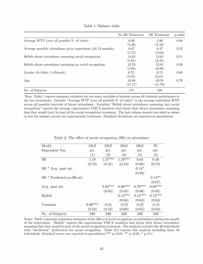
Table 1 shows that all pre-experiment outcomes as well as preferences elicited through our entry
survey are balanced across YMCA members who participated in Grow & Thrive with or without
social recognition.24 In the thirteen months preceding the experiment, participants on average
attended 6.67 times each month (for our two treatments with and without social recognition,
respectively 6.47 and 6.87 (p = 0.52).25 Overall, 73% of participants were female, and the average
age was 44.
23While we believe these responses are due to lack of attention when filling out the survey, we do acknowledge thepossibly that some individuals may have these preferences. For example, there could be modest individual(s) who donot want to be socially recognized far away from average attendance, but do not mind as much being observed closerto the mean population.
24Online Appendix Table H.1 shows a balance table for the full sample, including the incoherent individuals.25Moreover, the pre-trends are very similar for both participants and non-participants, as seen in Online Appendix
E.
15
4.2 The effect of social recognition on behavior
Figure 2 displays the cumulative distribution functions of attendance by treatment, showing that
the impact of social recognition is positive across all levels of attendance. We quantify these results
in Table 2.26 Column (1) of Table 2 reports a simple OLS regression on whether individuals
received the randomized social recognition treatment. The regression shows that social recognition
increased attendance by 1.19 visits (p = .105), which constitutes a 17% precent increase from the
6.96 attendances in the control group. In column (2) we control for past attendance, which is highly
correlated with treatment month attendance (ρ = 0.78, p < 0.001) and thus shrinks standard errors
significantly. Controlling for past attendance increases our estimate to 1.57 attendances27 (p =
0.001), which constitutes a 23% increase above control group attendance. Column (3) replicates
column (2) while also controlling for individuals’ beliefs about their attendance during the treatment
month assuming that they would be part of the social recognition treatment.28
Finally, in columns (4) and (5) we explore treatment effect heterogeneity. Column (4) reports
a regression that interacts the treatment effect of social recognition with past attendance. The
regression shows that the impact of social recognition is increasing by 0.14 attendance per past
attendance (p = 0.067) and that social recognition does not have much of an impact on members
with zero prior attendances. Given the tight correlation between past attendance and treatment
month attendance, this suggests that the treatment effect of social recognition is mostly multiplica-
tive. That is, social recognition increases attendance by a constant multiple of what attendance
would have been in the absence of social recognition. We formally estimate and test such a model
in column (5) by instrumenting the interaction between treatment and current attendance with
the interaction between treatment and past attendance. We estimate that the treatment effect of
social recognition is 14% (p = 0.048) of what attendance would have been in the absence of social
recognition. Overall, these results indicate that social recognition causally increased attendance at
the YMCA by between 17-23%.
4.3 The reduced-form social recognition function
We now estimate the utility from social recognition by analyzing individuals’ WTP to receive (or
avoid) social recognition. Our approach permits within-subject identification by eliciting partici-
pants’ WTP for social recognition conditional on all possible number of attendances. This directly
and non-parametrically identifies what we called the reduced-form social recognition function Rexp
in Section 2.
Figure 3 plots how WTP depends on the attendance level for the whole sample of coherent
participants, and also for YMCA members whose attendance prior to the experiment is above
or below median (5.1 visits per month). We plot the average WTP against the midpoint of the
26Table H.2 shows that the results are robust to using the full sample.27Recall that the untreated group had slightly higher past attendance, and thus a slightly higher propensity to
attend the YMCA during treatment month.28The results are identical when controlling for individuals’ beliefs about their attendance during the treatment
month assuming that they would not be part of the social recognition treatment
16
attendance interval for which it was elicited.29 The figure shows that WTP for social recognition
is increasing in the number of visits to the YMCA, consistent with both of the models summarized
in Section 2. Utility ranges from -$1.70 for zero attendances to $2.61 for twenty-three or more
attendances. As is apparent, these results do not depend at all on whether individuals have above-
or below-median attendance.
Figure 4 plots the ex-post utility from social recognition that each individual receives, together
with a quadratic fit. If an individual attended a times during treatment month, and had a WTP
for social recognition of R(a), then we assign social recognition utility R(a) to this individual. This
figure looks much like Figure 3, which is unsurprising given that Figure 3 suggests that there is
little heterogeneity in the social recognition function by one’s propensity to attend the YMCA. A
useful feature revealed by Figure 4, which we will utilize in our structural estimation, is that the
reduced-form social recognition function is well approximated by a quadratic function.
We quantify the reduced-form social recognition function in Table 3. Columns (1) and (2)
present OLS regressions of linear and quadratic fits, and show that WTP for social recognition is
increasing and concave in the number of visits. Columns (3) and (4) replicate this analysis with
Tobit regressions, which account for the fact that participants in our experiment could not express
WTP below -$8 or above $8.
In Table 4 we examine the degree of heterogeneity in the reduced-form social recognition func-
tion, using both OLS and Tobit regressions with linear and quadratic terms for past attendance.
As visually suggested by Figure 3, columns (1) and (2) show that there is little difference in the
social recognition functions of those with above versus below median past attendance. Column
(3) analyzes this further by interacting past attendance with the coefficients on attendance and
attendance squared. The interactions are tightly estimated zeroes, while the coefficients on at-
tendance and attendance squared remain largely unchanged compared to column (4) of Table 3.
We find very similar results for the tobit (columns 4 to 6). This provides strong evidence that
the social recognition function does not vary with individuals’ propensity to attend the YMCA.30
We use this fact in in our structural estimation of the impacts of applying our social recognition
intervention to the whole YOTA population, which has a somewhat lower average attendance than
the experimental population.31
Finally, we observe that the reduced-form social recognition function estimated here is consistent
with the action-based model. The action-based model predicts that SR utility should equal zero
at the population average, which was 3.16 attendances for the YOTA population during Grow &
29As noted in Section 3.3, the intervals of possible visits were the following: 0 visits, 1 visits, 2 visits, 3 visits, 4visits, 5 or 6 visits, 7 or 8 visits, 9 to 12 visits, 13 to 17 visits, 18 to 22 visits, and 23 or more visits.
30To be clear, we mean the social recognition function—not the social recognition utility a person ends up obtainingex-post at the end of the treatment month.
31In Online Appendix F we examine the relationship between social recognition functions and other demographics.Wald tests for the OLS and Tobit models suggest that there isn’t much of an interaction (p = 0.06 and p = 0.16,respectively), although there is some evidence that women have a less concave social recognition function. Becausewomen are somewhat over-represented in our experiment, this would imply that our out-of-sample estimates ofdeadweight loss would slightly underestimate it.
17
Thrive.32 Figures 3 and 4 both show that social recognition payoffs are approximately zero at 3
attendances. Both the OLS and Tobit models estimated in Table 3 cannot reject that that social
recognition is indeed zero at 3.16 attendances (p = 0.45 and p = 0.98, respectively).
5 Structural estimates of models and deadweight loss
Our results thus far provide us with a non-parametric estimate of the reduced form social recognition
functionRexp, and provide strong evidence of concavity. This qualitative finding of concavity implies
that social recognition will generate deadweight loss.
In this section, we build on this qualitative finding in two ways. First, we structurally estimate
the underlying social recognition utility functions. Second, we use those estimates to quantify the
degree of deadweight loss. In particular, we estimate the impact of applying our social recognition
intervention to the whole population of the YMCA of the Triangle Area (YOTA).
Throughout, we make the natural assumption that individuals care about how they are seen
relative to the broader YOTA population. For the action-based model, this implies the reference
point is the average attendance of the YOTA population. This assumption is well supported by
our reduced-form results that WTP at the average YOTA attendance is approximately zero.
For the type signaling model, note that individuals who are not socially recognized for their
particular attendance level are not recognized for being part of the experiment, and thus an ob-
server’s expectation of their type can only be that it is the mean of the broader population. Thus
the nature of the experimental design implies that an individual’s WTP for social recognition must
be the difference between the image utility of having their type revealed and the image utility of an
observer simply believing that they are part of the broader population. This implies that behavior
corresponding to that of the “average type” should generate the same social recognition payoffs as
if nothing about that individual’s behavior were observed.
Although natural, these assumptions complicate analysis because they imply that behavior
in our experiment is partial equilibrium behavior. A successful social recognition intervention
shifts the equilibrium, and thus the social recognition payoffs tied to any one particular action.
For example, individuals who evaluate their behavior relative to the average would have a more
demanding average to compare to, since a broadly applied social recognition intervention would
increase everyone’s behavior. Consequently, the function Rexp cannot be directly used to quantify
what deadweight loss from social recognition would be in a full equilibrium. Our strategy is therefore
to use the experimental data to estimate the structural social recognition function S, and use that
to quantify the equilibrium effects of applying social recognition to the YOTA population.
The key assumption for our out-of-sample estimates to be unbiased is that conditional on past
attendance, selection into our experiment is uncorrelated with social recognition utility functions.
Concretely, the question we answer is thus this: given the distribution of past attendance of the full
32This was (unsurprisingly) very close to the prior average month’s average of approximately 3 attendances, whichwe communicated to participants in our experiment.
18
YOTA population, but assuming that conditional on past attendance the experimental and the full
population have the same utility functions, what would be the deadweight loss of applying social
recognition to this full population. For the purpose of quantitatively interpreting our reduced-form
results about concavity, we view an answer to this potentially more narrow question as informative
as well. Even for this more modest out-of-sample exercise to be valid, however, we must still still
rely on the assumption, strongly supported by Table 4, that social recognition utility functions do
not vary by one’s propensity to attend the YMCA.
5.1 Assumptions and parameters for model estimation
Material utility
We normalize the material utility function such that an individual’s choice of attendance absent
social recognition or other incentives is simply his type θ. We also assume that individuals with
θ = 0 choose a = 0 and are inelastic to both social recognition and financial incentives, but that
the function is continuous in θ > 0. The existence of a large mass of θ = 0 types is motivated by
the empirical distribution of attendance.33 This normalization allows us to recover the distribution
of types in the population non-parametrically, simply by observing the distribution of attendance
in the broader YOTA population. These assumptions are satisfied by the functional form u(a; θ) =
a− a2
2θ .
Social recognition utility
Motivated by our reduced-form results and the quadratic fit in Figure 4, we assume that the
reduced-form social-recognition function Rexp in the experiment is quadratic. In the action-based
model, this assumption implies then S is given by β1(a− a)− β2
2 (a− a)2,34 and thus Rexp is given
by
Rexp(a) = γ1a−γ2
2a2 −
(γ1a0 −
γ2
2a2
0
), (3)
where a0 is the attendance of the whole YOTA population that month, and where γ2 = β2 and
γ1 = β1 + γ2a0. Notably, Rexp has only two free parameters: γ1 and γ2.
To study the implications of the type-based model, recall the assumption that S(θ, θ) = 0,
where θ is the average of the broader YOTA population. Define a∗exp(θ) as the optimal action
choice of a type θ in the experiment. When combined with our normalization assumption that
individuals choose a = θ in the absence of social recognition, this implies that Rexp must equal zero
33In the data, 39-51% of members attend 0 times on any given month. And conditional on not attending in theprior month and remaining a member, the likelihood of attending in the current month is only 19%.
34Since we assume that S is increasing, we technically have S = max(s, β1(a − a) − β22
(a − a)2), where s =
maxa(β1(a− a)− β2
2(a− a)2
). This means that S is strictly increasing for all a satisfying β1 − β2(a− a) ≥ 0 and is
flat thereafter. The estimates of β1 and β2 that we obtain imply that S is, in fact, strictly increasing for all possibleattendance levels a ≤ 31 both in the experiment and in the counterfactual equilibrium that would result if socialrecognition were applied to the whole population.
19
at a∗(θ) = a∗(a0). Thus Rexp under social recognition utility must have the form
Rexp(a) = γ1a−γ2
2a2 −
(γ1a∗(a0)− γ2
2a∗(a0)2
). (4)
Appendix B provides the derivations for the structural social recognition function S(θ; θ) that
generates the quadratic reduced-form social recognition function as above. There, we formally
derive the separating equilibrium, and we show that S is concave and approximately quadratic in
θ as well.
The parametric form of total utility
Our normalization assumptions on total utility U = a − a2
2θ + Rexp(a) imply that Rexp is in units
of “utils” rather than in units of money, as in WTP data. It will thus be convenient to write
Rexp(a) = ηRexp(a), where η is the marginal utility of money and Rexp(a) is the social recognition
utility in units of dollars. We will define R(a) := γ1a− γ2
2 a2 − γ0, so that γ1 = ηγ1 and γ2 = ηγ2.
Intuitively, the parameters γ1 and γ2 are revealed by our data on WTP for social recognition
at different levels of attendance, while the parameter η is revealed by our estimate of how much
social recognition actually affects behavior, given our monetization of the social recognition utility
function. To see the second point concretely, note that the attendance of a type θ receiving social
recognition in the experiment is given by
a∗exp(θ) = θ1 + ηγ1
1 + θηγ2(5)
≈ θ(1 + ηγ1) (6)
That is, social recognition increases attendance by a fraction of approximately ηγ1. The approxi-
mation in equation (6) holds when γ2 is small relative to γ1 (and when θ is not too large), which
we will estimate to be the case. This approximation coincides with our empirical results that the
effects of social recognition are approximately a constant fraction of what attendance would be in
the absence of social recognition.
The distribution of types
The distribution of types θ in the YOTA population is revealed non-parametrically by the distribu-
tion of their attendance. This follows directly from our normalization assumptions on the material
utility function.
5.2 Moment conditions for model parameters
The key parameters we must estimate are γ1, γ2 and η. We do this via generalized method of
moments (GMM). Equations (3) and (4) for the action-based and type-based models, respectively,
20
lead to three moment conditions of the form
E[Rexp(ai) · aki
]= 0
for k = 0, 1, 2. Given η and a0 these moments identify γ1 and γ2 , analogous to the regressions in
Table 3.
Next, equation (5) implies the moment condition
E
[ai + aiηγ1
1 + aiηγ2− ai|i ∈ control
]= τSR
for individuals i in the control group, where τSR is the average treatment effect of social recognition.
Given τSR and γ1 and γ2, this moment identifies η. To obtain τSR with, we set-up moment conditions
corresponding to the regression in column (2) of Table 2, which controls past behavior apasti . These
three moment conditions are simply
E[ai − τSR − b · apasti − a0,exp
]= 0
E[(ai − τSR − b · apasti − a0,exp
)apasti
]= 0
E[(ai − τSR − b · apasti − a0,exp
)1SR
]= 0
where 1SR is an indicator for being randomized into the social recognition treatment and a0,exp is
the average attendance of those in the experimental population not treated with social recognition.
Together, this yields seven moment conditions for a vector of six parameters: γ1, γ2, η, τSR, b
and a0,exp. The overidentification is a consequence of the restrictions that both the action-based
and type-based models impose on the constant term in equations (3) and (4), which restrict it to
be a function of γ1 and γ2.
Letting ξ := (γ1, γ2, η, τSR, b, a0,exp) denote the parameters, the GMM estimator chooses the
parameters ξ that minimize(m(ξ)−m(ξ)
)′W(m(ξ)−m(ξ)
), where m(ξ) are the theoretical
moments, m(ξ) are the empirical moments, and W is the optimal weighting matrix given by the
inverse of the variance-covariance matrix of the moment conditions. We approximate W using a
two-step estimator outlined in Hall (2005). In the first step, we set W equal to the identity matrix,35
and use this to solve the moment conditions for ξ, which we denote ξ1. Since ξ1 is consistent, by
Slutsky’s theorem the sample residuals u will also be consistent. We then use these residuals to
estimate the variance-covariance matrix of the moment conditions, S, given by Cov(zu), where z are
the instruments for the moment conditions. We then minimize(m(ξ)−m(ξ)
)′W(m(ξ)−m(ξ)
)using W = S−1, which gives the optimal ξ (Hansen, 1982).
35One other common approach is to use (zz′)−1as the weighting matrix in the first-stage, where z is a vector ofthe instruments in the moment equations. We confirmed our standard errors and point estimates are the same underboth choices.
21
5.3 Equilibrium predictions
The parameters γ1 = ηγ1 and γ2 = ηγ2 allow us to compute the equilibrium effects of applying
social recognition to the full population. The action-based and type-based models, however, impose
different requirements for inferring equilibrium behavior and deadweight loss from Rexp, which we
work through below.
Action-based model
The structural action-based model is S(a; a) = β1(a − a) − β2
2 (a − a)2, where the βi are obtained
from γi through the identities β2 = γ2 and β1 = γ1− γ2a0. To derive the equilibrium consequences
of applying social recognition to the whole YOTA population we must therefore compute what a,
average attendance, would be in equilibrium. Applying social recognition to the whole population
raises attendance and thus a. This raises the standard for “good” attendance, which in turn
increases the marginal social recognition payoffs from increasing a. Indeed, ∂∂aS = β1 + β2(a− a),
which is increasing in a.
To solve for equilibrium a, we note that a type θ’s optimal choice of action given a is a∗(θ) =
θ 1+β1+β2a1+θβ2
. Equilibrium average attendance must therefore satisfy
a = E
[θ
1 + β1
1 + θβ2
]+ aE
[θβ2
1 + θβ2
]. (7)
Because equation (7) is linear in a, it has a unique solution, and thus the equilibrium of the
action-based model must be unique. Equation (7) implies that equilibrium average behavior is
given by
aE =(1 + β1)E
[θ
1+θβ2
]1− β2E
[θ
1+θβ2
]Type-based model
In contrast to the action-based model, the type-based model implies that Rexp = Rpop. That is, the
reduced-form social recognition utility function we estimate for the experimental population would
be the same one that applies in an equilibrium in which social recognition is scaled up to apply to
everyone in the population. This is for two reasons. First, both the experimental population and
the broader population are assumed to care about how they compare to the average type θ in the
population. Unlike equilibrium average attendance a, θ is a primitive of the model that does not
change.
Second, because we have an (approximately) continuous strategy space, the equilibrium in our
model is a separating equilibrium, in which each type θ’s optimal choice of action depends on the
structural social recognition function S and on θ, but not on any other moments of the distribution
of θ (see Appendix B). This implies that even though the types θ that are in the experiment are
22
not representative of those in the population, the equilibrium choice of action of any give type θ
will be the same.
The property that a type θ’s choice of action is independent of the distribution of types (beyond
θ) generally holds for any signaling model with a continuous action space and a utility function that
satisfies the “single-crossing” property (Mailath, 1987). When the action space is not continuous,
however, this property generally does not hold for signaling models; see, e.g., Benabou and Tirole
(2006) for insightful implications of this for the case of binary actions. Our continuous action
space is thus crucial not only for making direct inferences about the shape of the social recognition
function, but also for making valid out-of-sample predictions for type-based signaling models.
Deadweight loss
We compute un-normalized deadweight loss as E[Rpop(a∗i )], where a∗i is the action chosen by indi-
viduals in equilibrium when social recognition is applied to the whole YOTA population. We also
compute the equivalent price metric by computing for each individual i, the reward per attendance
pi that would induce them to choose a∗i in the absence of social recognition. The first order condi-
tion for the optimal action in the absence of social recognition is ai = θi(1 + pi) in the absence of
social recognition.36 Since by definition this must equal individuals, attendance in the presence of
of social recognition, we have
1 + pi =aSRiθi
=1 + ηγ1
1 + θηγ2(8)
where aSRi is attendance in the presence of social recognition (but no piece-rate incentives).37
5.4 Results
Table 5 presents our estimates. Panel 5a presents the estimates of the main parameters γ1, γ2 and
η. For the action-based social recognition function, the parameter estimates imply S = 0.45(a −a) − 0.01(a − a)2.38 For the type-based social recognition function, the results in ppendix B give
us the approximation S(θ, θ) ≈ 0.47(θ − θ) − 0.02(θ − θ)2.39 All standard errors are clustered at
36Specifically, let pi(θ) denote the per-attendance price given to consumer i that lets them achieve the same levelof attendance a∗ as in social recognition. Then (suppressing θ for convenience) each individual’s utility is given byU(θ) = a− 1
2θa2 + pa. We can then use this to explicitly solve for p as a function of a∗ (and hence of θ). By taking
the FOC with respect to a:
0 = 1− 1
θa+ p
p =a
θ− 1
So to induce attendance a∗, an individual would need to be offered a price p such that p = a∗
θ− 1 = a∗
a− 1
37We exclude individuals with zero attendance from the average price metric, as this metric is undefined for them.38From section 5.3, we have S(a; a) = β1(a − a) − β2
2(a − a)2. Using β1 = ηγ1 − ηγ2a0 and β2 = ηγ2, we can
rewrite this as S(a; a) = (ηγ1 − ηγ2a0)(a − a) − ηγ22
(a − a)2. We then substitute a0 = 3.16 and the estimates fromTable 5a, η = 1.32, γ1 = 0.41, and γ2 = 0.02, to obtain the result.
39From equation 9, we have S(θ; θ) ≈(γ1(1 + γ1)− θγ2(1 + γ1)2
)(θ − θ) − γ2(1+γ1)2
2(θ − θ)2. The results
in Appendix B imply θ(1 + γ1) = a0. Substituting this and γ1 = ηγ1, γ2 = ηγ2 into S yields S(θ; θ) ≈
23
the subject level, and are based on the variance-convariance matrix computed using the efficient
two-step GMM estimator described in Section 5.2.
Panel 5b utilizes the parameter estimates from panel 5a to present estimates of deadweight loss,
behavior change, the equivalent price metric, and the normalized deadweight loss values. Because
the statistics in panel 5a are highly nonlinear functions of the parameters in panel 5a, we compute
95% confidence intervals without relying on asymptotic normality approximations. Instead, we
compute our confidence intervals using percentile-based bootstrap blocked at the individual level.
In Appendix G we show that our bootstrapped confidence intervals are nearly identical to those
computed analytically from asymptotic normality approximations for all but the normalized dead-
weight loss estimates. Using bootstrap simulations, we show that this is because the distributions of
the normalized deadweight loss estimates are not well approximated by normal distributions, which
implies that the first-order approximation utilized by the delta method has to perform poorly.
Column (1) in Table 5b presents the un-normalized deadweight loss estimates, while column (2)
presents the change in attendance that would result if the attendance of everyone in YOTA were
socially recognized. The estimates in column (2) imply a 19-23% increase in attendance, which
closely matches our reduced-form estimate of a 23% increase on the experimental population,
despite the two populations having different baseline attendance. The approximation in equation
(6), which shows that social recognition has an approximately proportional effect, clarifies why our
two estimates of percent increases are so similar.
Column (3) shows that the deadweight loss per extra attendance is 0.45 (CI 0.27-0.89) and 0.58
(CI 0.23-1.31) for the action-based and type-based models. Column (4) shows that on average, the
effects of social recognition are equal to piece-rate incentives of $0.36 and $0.27 in the action-based
and type-based models. Column (5) combines these estimates to produce deadweight loss per dollar
of behaviorally-equivalent incentives. We find this to be $1.23 for the action-based model and $2.15
for the type-based model. On the whole, these results are consistent with significant concavity in
the social recognition utility function, which produces significant deadweight loss.
These results also underscore the importance of working through the microfoundations of social
recognition utility. While both models produce estimates in the same ballpark, they are still
meaningfully different. One reason for this is that the action-based model predicts more behavior
change because of equilibrium adjustment that does not occur in the type-based model.
6 Misprediction of own behavior and its implications
A key and innovative feature of our design is that our elicitation of people’s WTP for social
recognition does not require them to form beliefs about their future attendance. This design feature
was motivated by growing evidence that individuals may hold incorrect beliefs about their future
behavior (e.g., DellaVigna and Malmendier, 2006; Grubb, 2009, 2015) In Figure 5, we assess the
2(θ − θ)2. We then substitute a0 = 3.16 and the estimates
from Table 5a, η = 1.11, γ1 = 0.35, and γ2 = 0.02, to obtain the result.
24
accuracy of individuals’ beliefs. We find that on average, individuals overestimate their attendance
by 35% (p < .05). Such misprediction has several important implications, which we discuss below.
6.1 Implications for experimental design
First, the possibility of misprediction implies that “strategy method” designs such as ours are
crucial for avoiding biases in individuals’ valuations of non-price levers. Consider the alternative
design strategy of simply eliciting WTP for being part of the social recognition program, with-
out conditioning on attendance. Because social recognition utility is monotonic in attendance,
overestimation of one’s future attendance would then lead one to overestimate the expected social
recognition utility one would derive. An analyst taking those WTPs at face value might then
conclude that social recognition is in fact positive-sum, rather than negative-sum as we find.
Such strategy-method designs are crucial beyond work evaluating social recognition schemes.
For example, applying our design strategy to an experiment such as that of Allcott and Kessler
(2019) would allow for estimates of the utility effect of conserving more or less energy than one’s
neighbors, without having to assume that people can accurately forecast their future energy use.
6.2 Implications for market structure
Incorrect beliefs about future behavior may lead individuals to overestimate the utility they may
obtain from a social recognition scheme. This overestimation can significantly effect market struc-
ture. As we discuss in the introduction, social recognition programs are frequently used by busi-
nesses to incentivize high performance among their employees . However, individuals’ evaluations
of workplaces with particularly aggressive social recognition programs would be upwardly biased if
individuals overestimate their likelihood of being recognized for good performance. In line with the
reasoning of behavioral IO models studying the implications of misprediction of behavior (DellaV-
igna and Malmendier, 2004), and of shrouded attributes (Gabaix and Laibson, 2006; Heidhues et
al., 2016), such overestimation can lead firms to use social recognition programs even when they
are negative-sum. This would result in inefficient incentive structures.
7 Limitations, robustness, and conclusions
A recent and growing literature establishes that public recognition of behavior can have large effects
in a number of economically consequential field settings. We build on this literature by developing
a framework for quantifying the social efficiency of using social recognition for behavior change. We
show theoretically that a simple indication of whether social recognition programs are more socially
efficient than traditional financial incentives is the shape of the social recognition utility function—if
it is concave (convex), then social recognition is negative-sum (positive-sum). Although it is often
assumed that one’s social recognition utility is linear in the audience’s inferences about one’s type
(e.g., Benabou and Tirole 2006, 2011; Ali and Benabou 2016), we show that this assumption is
far from innocuous for questions about the efficiency of social recognition interventions. We then
25
develop experimental techniques that permit robust and direct elicitation of the social recognition
utility function for individuals in the experiment, including a direct estimate of the curvature of
this function. And we develop structural methods that allow us to analyze—taking into account
the equilibrium effects—the behavioral and social efficiency consequence of scaling up the social
recognition intervention beyond the experimental sample.
We implement our approach with the YMCA of the Triangle Area. We estimate that publicizing
the attendance of all members of these branches would increase attendance by about 20%, but would
generate deadweight loss of $1.23-$2.15 per dollar of behaviorally-equivalent financial incentives.
This suggests that social recognition may not compare favorably to financial incentives as a means
of creating behavior change. Beyond the immediate policy implications, this finding also suggests
that, because of individuals’ overly optimistic beliefs, a competitive market could overuse social
recognition schemes.
That said, a number of caveats are in order.
First, our deadweight loss quantification should not be interpreted as a holistic assessment of
the welfare effects. Even if there is significant deadweight loss, the social benefits from behavior
change may be large, and thus a social recognition intervention may yield large and positive welfare
effects compared to doing nothing. Rather, our research question is about the welfare effects of
social recognition, holding constant the benefits from behavior change. Answering such a question
for an arsenal of different possible levers for behavior change provides a direct comparison of which
tools are most efficient in bringing about the desired behavior change.
Second, while our deadweight loss concept builds on classical tools and concepts in public
finance, practical applications of our framework may be tempered by political economy constraints.
In some settings, it may be more politically acceptable to rely on non-price interventions such
as social recognition rather than on financial incentives. And because, as we note above, the
welfare effects of behavior change may be large, social recognition may be an attractive second-best
solution. But even in such settings, our framework helps provide an answer to how socially costly
those political economy constraints are, and how important it may be to try to relax them.
Relatedly, the set of possible financial incentive schemes may be limited. We have shown that
social recognition provides the highest marginal incentives for the lowest types by virtue of being
a concave function. To the extent that targeting such low types is desirable, social recognition
may have an attractive targeting property over financial incentives if political economy or practical
considerations limit to linear incentive schemes. In this case our framework would be used to weight
the benefits of targeting against the efficiency costs of relying on a negative-sum lever.
Third, we emphasize that our results constitute only an initial data point on the efficiency
of social recognition levers. We conducted our study on a selected sample that is not fully rep-
resentative of the U.S. population, and thus our broad conclusions about the deadweight loss of
social recognition must be interpreted with caution. To the extent that curvature of the social
recognition utility function may vary meaningfully over the population, our quantitative estimates
may not hold in other contexts. Whether it is plausible that curvature may vary substantially
26
across different populations is a question for future research. Variation in the sensitivity to social
recognition poses a smaller problem, particularly for our normalized deadweight estimates. Since
sensitivity scales both the change in behavior and the WTP to be socially recognized, variation in
sensitivity is not likely to have a big effect on our conclusions about normalized deadweight loss.
Fourth, the core reasons for why individuals derive utility from social recognition matter. We
believe that our experiment mostly channels an intrinsic desire to appear “good,” as do many other
settings. In some contexts, however, the information revealed about individuals directly affects
their material payoffs. Plainly, our results about the intrinsic motives are not informative about
the shape of utility from extrinsic motives in such settings.
Fifth, our quantitative estimates cannot be directly applied to social recognition schemes that
produce different information structures; e.g., ones that recognize only if people are at the top or
not. However, as we show in Section 2, any information structure will generate deadweight loss
if the structural social recognition function is concave, and social efficiency gains if it is convex.
Thus, all else equal, different information structures would not change our qualitative result, and
would probably not have a big affect the normalized deadweight loss estimates.
Finally, despite a novel feature of our design that eliminates the need to (incorrectly) assume
rational expectations of future behavior, our elicitation method is not immune from all possible
forecasting biases. In particular, individuals may misforecast the intensity of feelings of pride or
shame, conditional on a particular realization of behavior. Testing this possibility would require a
very data-intensive design that elicits peoples WTP for social recognition after their attendance is
realized. Such an approach would require an order of magnitude more data than ours, and is thus
left for future research.
Despite the open questions and the weaknesses of our approach that we hope future work will
evaluate and address, our approach nevertheless provides a tractable toolkit for evaluating non-
price levers. Although non-price interventions such as “nudges” have become popular tools among
governments around the world (Thaler and Sunstein, 2008; OECD, 2017), there is little rigorous
economic analysis of the actual welfare effects of such interventions (Bernheim and Taubinsky,
2018). Extending the core frameworks of public economics to consider non-price interventions is
crucial for robust and holistic welfare analysis.
References
Al-Ubaydli, Omar, John A List, Danielle LoRe, and Dana Suskind, “Scaling for Economists:Lessons from the non-adherence problem in the medical literature,” Journal of Economic Perspectives,2017, 31 (4), 125–44. 2.3
Ali, S. Nageeb and Roland Benabou, “Image versus information: Changing societal norms and optimalprivacy,” Working Paper 22203, National Bureau of Economic Research 2016. 1, 2.1.1, 2.1.2, 2.2, 7
Allcott, Hunt and Judd B Kessler, “The welfare effects of nudges: A case study of energy use socialcomparisons,” American Economic Journal: Applied Economics, 2019. Forthcoming. 1, 4, 11, 21, 6.1
27
Andreoni, James and B. Douglas Bernheim, “Social image and the 50–50 norm: A theoretical andexperimental analysis of audience effects,” Econometrica, 2009, 77 (5), 1607–1636. 1, 6, 2.1.2
Angrist, Joshua D and Jorn-Steffen Pischke, Mostly harmless econometrics: An empiricist’s compan-ion, Princeton University Press, 2008. G
Ariely, Dan, Anat Bracha, and Stephan Meier, “Doing good or doing well? Image motivation andmonetary incentives in behaving prosocially,” American Economic Review, 2009, 99 (1), 544–555. 5, 12
Ashraf, Nava, Oriana Bandiera, and B Kelsey Jack, “No margin, no mission? A field experiment onincentives for public service delivery,” Journal of Public Economics, 2014, 120, 1–17. 1, 12
Auerbach, Alan J., The theory of excess burden and optimal taxation, Elsevier, 1985. 2.2, A
Augenblick, Ned and Matthew Rabin, “An experiment on time preference and misprediction in un-pleasant tasks,” Review of Economic Studies, 2019. Forthcoming. 3.7
Banerjee, Abhijit, Rukmini Banerji, James Berry, Esther Duflo, Harini Kannan, ShobhiniMukerji, Marc Shotland, and Michael Walton, “From proof of concept to scalable policies: Chal-lenges and solutions, with an application,” Journal of Economic Perspectives, 2017, 31 (4), 73–102. 2.3
Barankay, Iwan, “Rankings and social tournaments: Evidence from a crowd-sourcing experiment,” Whar-ton School of Business, University of Pennsylvania Working Paper, 2011, pp. 1–38. 1
Becker, Gary S., “A Note on Restaurant Pricing and Other Examples of Social Influences on Price,”Journal of Political Economy, 1991, 99 (5), 1109–1116. 1, 2.1.1
Benabou, Roland and Jean Tirole, “Incentives and Prosocial Behavior,” American Economic Review,2006, 96 (5), 1652–1678. 1, 5, 6, 2.1.2, 5.3, 7
and , “Laws and Norms,” Working Paper 17579, National Bureau of Economic Research 2011. 1, 2.2,7
Bernheim, B. Douglas and Dmitry Taubinsky, Behavioral public economics, Vol. 1, Elsevier, 2018. 4,7
, Andrey Fradkin, and Igor Popov, “The welfare economics of default options in 401 (k) plans,”American Economic Review, 2015, 105 (9), 2798–2837. 1
Besley, Timothy and Stephen Coate, “Workfare versus welfare incentive arguments for work require-ments in poverty-alleviation programs,” American Economic Review, 1992, 82 (1), 249–61. 1, 2.1.1
Blomquist, N. Soren, “Interdependent behavior and the effect of taxes,” Journal of Public Economics,1993, 51 (2), 211–218. 1, 2.1.1
Bloom, Nicholas and John Van Reenen, “Measuring and explaining management practices across firmsand countries,” Quarterly Journal of Economics, 2007, 122 (4), 1351—1408. 1
Bø, Erlend E, Joel Slemrod, and Thor O Thoresen, “Taxes on the internet: Deterrence effects ofpublic disclosure,” American Economic Journal: Economic Policy, 2015, 7 (1), 36–62. 1
Bradler, Christiane, Robert Dur, Susanne Neckermann, and Arjan Non, “Employee recognitionand performance: A field experiment,” Management Science, 2016, 62 (11), 3085–3099. 1
Bursztyn, Leonardo and Robert Jensen, “How Does Peer Pressure Affect Educational Investments?,”Quarterly Journal of Economics, 2015, 130 (3), 1329–1367. 1
and , “Social Image and Economic Behavior in the Field: Identifying, Understanding, and ShapingSocial Pressure,” Annual Review of Economics, 2017, 9 (1), 131–153. 1
28
, Bruno Ferman, Stefano Fiorin, Martin Kanz, and Gautam Rao, “Status goods: experimentalevidence from platinum credit cards,” Quarterly Journal of Economics, 2017, 133, 1561–1595. 1
, Georgy Egorov, and Robert Jensen, “Cool to be Smart or Smart to be Cool? Understanding PeerPressure in Education,” Review of Economic Studies, 2019. Forthcoming. 1, 5
, Thomas Fujiwara, and Amanda Pallais, “’Acting Wife’: Marriage Market Incentives and LaborMarket Investments,” American Economic Review, 2017, 107 (11), 3288–3319. 1
Carroll, Gabriel D, James J Choi, David Laibson, Brigitte C Madrian, and Andrew Metrick,“Optimal defaults and active decisions,” Quarterly Journal of Economics, 2009, 124 (4), 1639–1674. 1
Damgaard, Mette Trier and Christina Gravert, “The hidden costs of nudging: Experimental evidencefrom reminders in fundraising,” Journal of Public Economics, 2018, 157, 15–26. 1
Davis, Jonathan, Jonathan Guryan, Kelly Hallberg, and Jens Ludwig, “The economics of scale-up,” Technical Report, National Bureau of Economic Research 2017. 2.3
DellaVigna, Stefano, “Structual Behavioral Economics,” in B. Douglas Bernheim, Stefano DellaVigna,and David Laibson, eds., Handbook of Behavioral Economics, number 1, Elsevier, 2018. 1
and Ulrike Malmendier, “Contract design and self-control: Theory and evidence,” Quarterly Journalof Economics, 2004, 119 (2), 353–402. 6.2
and , “Paying not to go to the gym,” American Economic Review, 2006, 96 (3), 694–719. 6
, John A List, and Ulrike Malmendier, “Testing for altruism and social pressure in charitable giving,”Quarterly Journal of Economics, 2012, 127 (1), 1–56. 1, 6
, , , and Gautam Rao, “Voting to tell others,” The Review of Economic Studies, 2017, 84 (1),143–181. 1, 6, 11
Duflo, Esther, Rachel Glennerster, and Michael Kremer, “Using randomization in developmenteconomics research: A toolkit,” Handbook of development economics, 2007, 4, 3895–3962. 2.3
Exley, Christine, “Incentives for Prosocial Behavior: The Role of Reputations,,” Management Science,2018, 64 (5), 2460–2471. 5
Gabaix, Xavier and David Laibson, “Shrouded attributes, consumer myopia, and information suppres-sion in competitive markets,” Quarterly Journal of Economics, 2006, 121 (2), 505–540. 6.2
Gauri, Varun, Julian C Jamison, Nina Mazar, Owen Ozier, Shomikho Raha, and Karima Saleh,“Motivating bureaucrats through social recognition: evidence from simultaneous field experiments,” 2018.1
Gerber, Alan S, Donald P Green, and Christopher W Larimer, “Social pressure and voter turnout:Evidence from a large-scale field experiment,” American Political Science Review, 2008, 102 (1), 33–48. 1
Gosnell, Greer K, John A List, and Robert Metcalfe, “A new approach to an age-old problem: solvingexternalities by incenting workers directly,” Technical Report, National Bureau of Economic Research2016. 12
Grubb, Michael D., “Selling to overconfident consumers,” American Economic Review, 2009, 99 (5),1770–1807. 6
, “Overconfident consumers in the marketplace,” Journal of Economic Perspectives, 2015, 29 (4), 9–36. 6
Hall, Alistair R., “Generalized Method of Moments,” 2005. 5.2
29
Hansen, Lars Peter, “Large sample properties of Generalized Method of Moments estimators,” Econo-metrica, 1982, 50 (4), 1029–1054. 5.2
Heidhues, Paul, Botond Koszegi, and Takeshi Murooka, “Exploitative Innovation,” American Eco-nomic Journal: Microeconomics, 2016, 8 (1), 1–23. 6.2
Imas, Alex, “Working for the warm glow: On the benefits and limits of prosocial incentives,” Journal ofPublic Economics, 2014, 114, 14–18. 12
Karing, Anne, “Social signaling and childhood immunization: A field experiment in Sierra Leone,” WorkingPaper 2019. 1, 5
Karlan, Dean and Margaret A McConnell, “Hey look at me: The effect of giving circles on giving,”Journal of Economic Behavior & Organization, 2014, 106, 402–412. 1
Kosfeld, Michael and Susanne Neckermann, “Getting more work for nothing? Symbolic awards andworker performance,” American Economic Journal: Microeconomics, 2011, 3 (3), 86–99. 1
Lindbeck, Assar, Sten Nyberg, and Jorgen Weibull, “Social Norms And Economic Incentives In TheWelfare State,” Quarterly Journal of Economics, 1999, 114, 1–35. 1, 2.1.1
, , and Jorgen Weibull, “Social Norms and Welfare State Dynamics,” Journal of the EuropeanEconomic Association, 2003, pp. 533–542. 2.1.1
Loewenstein, George, Cass R Sunstein, and Russell Golman, “Disclosure: Psychology changeseverything,” 2014, 6, 391–419. 1
Mailath, George J, “Incentive compatibility in signaling games with a continuum of types,” Econometrica:Journal of the Econometric Society, 1987, pp. 1349–1365. 5.3, B
OECD, Behavioural Insights and Public Policy: Lessons from Around the World, OECD Publishing, 2017.7
Perez-Truglia, Ricardo and Guillermo Cruces, “Partisan interactions: Evidence from a field experi-ment in the united states,” Journal of Political Economy, 2017, 125 (4), 1208–1243. 1
and Ugo Troiano, “Shaming Tax Delinquents: Theory and Evidence from a Field Experiment in theUnited States,” Journal of Public Economics, 2018, 167, 120–137. 1
Thaler, Richard H and Cass R Sunstein, “Nudge: Improving decisions about health, wealth, andhappiness,” 2008. 7
Thunstrom, Linda, “Welfare effects of nudges: The emotional tax of calorie menu labeling,” Judgmentand Decision Making, 2019, 14 (1), 11–25. 1
WorldatWork, “Trends in Employee Recognition,” 2017. 1
Yoeli, Erez, Moshe Hoffman, David G Rand, and Martin A Nowak, “Powering up with indirectreciprocity in a large-scale field experiment,” Proceedings of the National Academy of Sciences, 2013, 110(Supplement 2), 10424–10429. 1
30
Figures and Tables
Figure 1: Illustration of social recognition information
Note: Figure shows the cumulative distribution function of attendance during the experiment across YMCAmembers in the social recognition treatment and the treatment without social recognition.
Figure 2: Cumulative distribution function of attendance during the experiment by treatment
0
.2
.4
.6
.8
1
0 10 20 30Attendance
No Social Recognition Social Recognition
Notes: Figure 2 shows the cumulative distribution function of attendance during the experiment acrossYMCA members in the social recognition treatment and the treatment without social recognition.
31
Figure 3: The reduced-form social recognition function (R)
-2
-1
0
1
2
3WTP ($)
0 5 10 15 20 25Visits
Avg. WTP Avg. WTP, at median past att.Avg. WTP, below median past att.
Notes: Figure 3 plots the average WTP for each of the eleven intervals of possible future attendances to theYMCA during the experiment. For intervals including more than one number of visits (e.g., “between 7 and8 visits”) the WTP is plotted at the average point of visits. The figure separately reports the average WTPfor the whole sample of coherent participants, and for coherent participants whose average attendance priorthe experiment was below/above the median past attendance.
32
Figure 4: Image payoffs by realized attendance during the experiment
-2
-1
0
1
2
3Social
RecognitionPayoff ($)
0 5 10 15 20Attendance during the experiment
Notes: Figure 4 presents a binned scatterplot of the WTP of each subject to receive social recognition attheir realized attendance level. The red line is a quadratic fit.
33
Figure 5: Beliefs about future attendance by attendance during the experiment
0
5
10
15
20
25Attendanceduring theexperiment
0 5 10 15 20 25Beliefs about future attendance
Notes: Figure 5 presents a binned scatterplot summarizing the relationship between the actual attendanceof subjects in the experiment and their beliefs about their attendance. For subjects in the social recognitiontreatment, their elicited beliefs about attendance the next month in the presence of social recognition areplotted. For subjects not in the social recognition treatment, their elicited beliefs about attendance the nextmonth absent social recognition are plotted.
34
Table 1: Balance table
No SR Treatment SR Treatment p-value
Average WTP (over all possible N. of visits) 0.98 1.06 0.88(5.26) (5.16)
Note: Table 1 reports summary statistics for our main variables of interest across all coherent participants inthe two treatments. Variable “Average WTP (over all possible N. of visits)” is the average individual WTPacross all possible intervals of future attendance. Variables “Beliefs about attendance assuming (no) socialrecognition” reports the average expectations YMCA members had about their future attendance assumingthat they would (not) be part of the social recognition treatment. The last column reports two sided p-valuesto test for balance across our experimental treatment. Standard deviations are reported in parentheses.
Table 2: The effect of social recognition (SR) on attendance
Model OLS OLS OLS OLS IVDependent Var. att. att. att. att. att.
(1) (2) (3) (4) (5)
SR 1.19 1.57*** 1.59*** 0.64 0.40(0.73) (0.45) (0.44) (0.68) (0.73)
SR * Avg. past att. 0.14*(0.08)
SR * Predicted no-SR-att 0.14**(0.07)
Avg. past att. 0.94*** 0.86*** 0.79*** 0.80***(0.04) (0.05) (0.06) (0.05)
Notes: Table 2 presents regression estimates of the effect of social recognition on attendance during the monthof the experiment. “Beliefs” reports the expectations YMCA members had about their future attendanceassuming that they would be part of the social recognition treatment. The analysis excludes the 46 individualswith “incoherent” preferences for social recognition. Table H.2 repeats this analysis including these 46individuals. Standard errors are reported in parentheses.*** p<0.01, ** p<0.05, * p<0.1.
35
Table 3: Willingness to pay for social recognition conditional on number of visits
Model OLS OLS Tobit TobitDependent Var. WTP WTP WTP WTP
(1) (2) (3) (4)
N. of visits 0.13*** 0.39*** 0.25*** 0.68***(0.01) (0.04) (0.03) (0.08)
N. of visits squared -0.01*** -0.02***(0.00) (0.00)
Note: Table 3 reports coefficient estimates from linear and quadratic models of willingness to pay for social recognitionat different numbers of visits. Columns (1) and (2) use OLS models while columns (3) and (4) use Tobit models. Theanalysis excludes the 46 individuals with “incoherent” preferences for social recognition. Table H.3 repeatsthis analysis including these 46 individuals. Standard errors, clustered at the subject level, are reported inparentheses. *** p<0.01, ** p<0.05, * p<0.1.
36
Table 4: Willingness to pay for social recognition conditional on number of visits—heterogeneityanalysis
Model OLS OLS OLS Tobit Tobit TobitDependent Var. WTP WTP WTP WTP WTP WTP
Sample ≥ Median < Median All ≥ Median < Median All
Note: Table 4 reports coefficient estimates from linear and quadratic models of willingness to pay for social recognitionat different numbers of visits. Columns (1) and (2) replicate Column (2) from 3, restricting the sample to subjectswho have above (below) median attendance during the fifty-four weeks prior to the experiment. Likewise, Columns(4) and (5) repeat Column (4) from 3, restricting the sample to subjects who have above (below) median attendanceduring the fifty-four weeks prior to the experiment. Columns (3) and (6) repeat Columns (2) and (4) from 3, butincluding interaction terms between past attendance and number of visits. The analysis excludes the 46 individualswith “incoherent” preferences for social recognition. Table H.4 repeats this analysis including these 46 individuals.Standard errors, clustered at the subject level, are reported in parentheses. *** p<0.01, ** p<0.05, * p<0.1.
Note: Panel 5a presents the GMM estimates from the moment conditions defined in 5.2. Standard errorsare clustered at the individual level, and are computed from the variance-covariance matrix derived from theefficient two-step estimator described in Section 5.2. Panel 5b presents the estimates for the counterfactualof enacting social recognition for the whole YMCA of the Triangle Area population. Column (1) presentsestimates of the DWL. Column (2) presents estimates of the average change in attendance, using equation(5). Column (4) presents estimates of the equivalent price metric, using equation(8).Bootstrapped percentile-based confidence intervals, sampled by subject with 1000 iterations, are reported in brackets for panel 5b.The analysis excludes the 46 individuals with “incoherent” preferences for social recognition. Table H.5repeats this analysis including these 46 individuals.
38
A General definition of deadweight loss
Consumers have utility given by U = u(a∗, y) + S, where y is their net earnings, and S is the
utility they derive from social recognition, as we defined in the body of the paper. Let Γ denote the
social recognition scheme, which consists of a visibility level ν as well as rules for what behaviors
are revealed or what signals are sent (e.g., all actions are revealed, or whether one is only a top
performer or not). We say Γ = ∅ if visibility is zero or if no information is revealed.
Let p denote a piece-rate incentive for behavior, such that choosing a produces financial rewards
of pa to the consumer. For each type θ, define the revenue-neutral incentive scheme CΓ(θ) =
(LΓ(θ), pΓ(θ)) such that pΓ > 0 and LΓ(θ) = −pΓ(θ)aΓ(θ), and such that C induces the effect on
type θ’s behavior as does Γ.40 Then we say that the deadweight loss of social recognition is how
much higher consumer surplus would be under incentives {CΓ(θ)} than under Γ. Our definition of
normalized deadweight loss is with respect to the average piece-rate incentives pΓ =∫θ∈Θ pΓ(θ)µ(θ),
where µ is the probability measure on types.
To formalize consumer surplus, we follow Auerbach (1985). Let a∗(p, Z,Γ; θ) denote the ac-
tion given piece-rate incentive p, wealth Z, transfer −L, and social recognition scheme Γ. Let
V (p, Z,Γ; θ) = u(a∗, Z,Γ; θ) +R(a∗) denote consumer’s indirect utility, where R(·) is the reduced-
form social recognition function mapping actions to utils. Generalizing the typical definition of
the consumer expenditure function, we define e(p,Γ; θ) as the minimum wealth necessary to obtain
utility V given a piece-rate incentive p and social recognition scheme Γ. The deadweight loss of
social recognition is
DWL(Γ) =
∫e(0,Γ; θ)µ(θ)−
∫e(pΓ, ∅; θ)µ(θ)
40Formally, such an incentive scheme always exists as long as substitution effects don’t overwhelm income effectsin the material utility function, an innocuous assumption that we make.
39
B Signaling model microfoundations
Define φ(θ) = θ(1+γ1)1+θγ2
. The structural social recognition function that leads to a quadratic reduced-
form social recognition function is given by S(θ, θ) = γ1φ(θ) − γ2
2 φ(θ)2 − s, where s = γ1φ(θ) −γ2
2 φ(θ)2. Note that for small values of θ, φ(θ) ≈ θ(1 + γ1), and thus S is approximately quadratic:
S ≈ γ1(1 + γ1)θ − γ2(1 + γ1)2
2θ2 − s.
Using the same approximation for θ, i.e., φ(θ) ≈ θ(1 + γ1),we can also see S is approximately
quadratic in θ − θ:
S ≈(γ1(1 + γ1)− θγ2(1 + γ1)2
)(θ − θ)− γ2(1 + γ1)2
2(θ − θ)2 (9)
We now show that an equilibrium action function is given by a∗(θ) = φ(θ). To see this, note
that if it were the case, then then the reduced-form social recognition function would be given by
R = γ1a − γ2
2 a2 − s. Given this reduced-form social recognition function, equation (5) gives that
each type θ’s optimal response is then simply
a∗ = θ1 + ηγ1
1 + θγ2
= φ(θ)
This shows that a∗(θ) = φ(θ) is, indeed, an equilibrium action function. Finally, because the
material utility function a− 12a2
θ satisfies the single-crossing property (the derivative with respect
to a, 1− aθ , is increasing in θ), the results of Mailath (1987) imply that this separating equilibrium
must be a unique separating equilibrium.
40
The remaining appendices are for online publication only
C Screenshots from the Experiment
Figure C.1: Invitation email to participate in Grow & Thrive
Figure C.1 shows a screenshot of the invitation email sent to YMCA members.
41
Figure C.2: Non-parametric elicitation of WTP: an example
(a) Strategy method
(b) BDM mechanism
Note: Figure C.2 shows a screenshot from our survey of the WTP elicitation for each number of possible visits tothe YMCA during the experiment. The example above reports the elicitation of WTP for attending one time. Thetop panel asks whether a participant wants to be socially recognized for attending one time. Participants make theirchoice by clicking their favorite option. The bottom panel asks how much a participant is willing to pay (from $0 to$8) to guarantee that his favorite option is implemented (notice that the bottom panel assumes that the participantanswered that he prefers not be recognized for attending one time). Participants choose the amount by moving theslider bar.
42
D Transcript of Frequently Asked Questions
FAQ – Grow & Thrive
Prepared for YMCA employees
Some general comments
If asked questions at the front desk, it is best if the front desk person says that he/she is aware of the Grow & Thrive program, but that she encourages the Y member to email questions to a specific person who can answer more thoroughly. For instance, the Y member inquiring could be provided with an email address.
Y staff should NOT reveal to Y members that they are part of an economic experiment. If Y members ask about why different people get different incentives, answer as per FAQ.
Below you will find a list of questions that YMCA members may ask, and the corresponding suggested answers.
Q: I have only completed the first part of the survey: will I still participate in drawing of $250 Y voucher? A: Yes
Q: I am curious: why are people randomized/assigned to the personal recogntion program and to receive extra rewards? A: Grow & Thrive is a pilot program: as such, we are evaluating different ways in which we might implement it on a larger scale in the future. [if the person insists:] We cannot provide further details at this moment.
Q: I have agreed to participate but now I don't want to be in the social recognition program: can you take me out of the social recognition program? A: By agreeing to participate in Grow & Thrive, you have also accepted the possibility to be randomly assigned by a computer lottery to participate in the social recognition program. If you do not want to be part of the social recognition program, you may withdraw from Grow & Thrive, in which case however you will also NOT receive any of the incentives of the program.
Q: Why is University of Chicago involved? A: University of Chicago scholars will help us evaluating our Grow & Thrive program and help us to improve it in the future.
Q: Is this an experiment? A: Grow & Thrive is a pilot program: if successful, we hope in the future to implement it on a larger scale to help our YMCA members live a healthier and fuller life.
43
Q: When will my donations be made? A: In July after the end of the Grow & Thrive program, we will email you with details on how the donations will be implemented. Q: During Grow & Thrive, do I have to check in with the front desk when I come to the Y? A: No, if you are part of Grow & Thrive, at the end of the month the Y staff will check how many times you came to the Y by counting the number of days you swiped your Y card to access the facilities. Q: How will I know if I won the $250 Y voucher? A: We will notify the winner of the drawing after the end of Grow & Thrive Q: If I win, will I receive the $250 in cash? A: You will receive it in the form of a discount on your future YMCA membership. Q: Who is providing the money for Grow & Thrive? A: An anonymous benefactor who has a strong passion for promoting healthy living and supporting the broader community. Q: Who else is participating in the social recognition program? A: I don't have this information at the moment, I am sorry. Q: In which group am I? [bits of this answer can also be used for people asking why they didn't get the extra reward, or why they are (are not) in the social recognition program despite their answers in the survey etc.] A: We will email you by June 15th to let you know which group you have been randomly assigned to. If you agreed to participate, with 10% chance a computer lottery will randomly select one of the answers you gave, and what you chose in that question will determine your program and reward. Otherwise, your program and reward will be randomly assigned to you: in this case you may or may not be part of the social recognition program. Q: What is the social recognition program again? A: Some Grow & Thrive members will also be part of a social recognition program. This group will receive at the end of the month a thank-you email, which will list their names and highlight the good that they have done for themselves by going to the Y during the month. The email will show how many times each participant of the social recognition program went to the Y during the 1-month Grow & Thrive. If you are not part of the social recognition program you will not receive nor be listed in this thank-you email. This is the only difference between being part or not of the social recognition program.
E Pre-trends in attendance by treatment group
Figure E.1 compares the average monthly attendance of the YMCA members for the treatment
group with social recognition to the treatment group absent social recognition.
44
Figure E.1: Attendance by treatment
Start of Exp.
0
1
2
3
4
5
6
7
8
9Averageattendance
May 15
- Jun
. 14,
2016
Jun.
15 - J
ul. 14
, 201
6
Jul. 1
5 - Aug
. 14,
2016
Aug. 1
5 - Sep
. 14,
2016
Sep. 1
5 - O
ct. 14
, 201
6
Oct. 15
- Nov
. 14,
2016
Nov. 1
5 - D
ec. 1
4, 20
16
Dec. 1
5 - Ja
n. 14
, 201
7
Jan.
15 - F
eb. 1
4, 20
17
Feb. 1
5 - M
ar. 14
, 201
7
Mar. 15
- Apr.
14, 2
017
Apr. 15
- May
14, 2
017
May 15
- Jun
. 14,
2017
Jun.
15 - J
ul. 15
, 201
7
Month
No Social Recognition Social Recognition
Figure E.1 shows the average monthly attendance of YMCA members in our two treatment groups during thethirteen months prior the experiment, and the month of the experiment..
F Reduced form SR function by member characteristics
Table F.1 repeats columns (2) and (4) of Table 3 including interactions with subjects’ age, gender (0
= male, 1 = female), average monthly past attendance, and donation to the last YMCA campaign.
In columns (2) and (4), we report the Wald Statistic for the test that the coefficients on all the
characteristics and their interactions with number of visits and number of visits squared are zero.
These statistics correspond to p-values of 0.06 and 0.16 respectively. Although the evidence that
the SR function varies by characteristics is weak, the results are suggestive that women have a less
concave SR function than men. Because women are over-represented in our experimental sample,
this implies that our deadweight loss estimates for the full YOTA population are slight lower bounds
45
Table F.1: Willingness to pay for social recognition conditional on number of visits—demographicanalysis
Model OLS OLS Tobit TobitDependent Var. WTP WTP WTP WTP
(1) (2) (3) (4)
N. visits 0.39*** 0.67*** 0.68*** 1.20***(0.04) (0.17) (0.08) (0.31)
N. visits squared -0.01*** -0.02*** -0.02*** -0.03***(0.00) (0.01) (0.00) (0.01)
Avg. past att. 0.04 0.07(0.06) (0.13)
N. visits * Avg. past att. -0.00 -0.01(0.01) (0.01)
N. visits sq. * Avg. past att. 0.00 0.00(0.00) (0.00)
Age -0.02 -0.04(0.03) (0.05)
N. visits * Age -0.00 -0.00(0.00) (0.01)
N. visits sq. * Age -0.00 -0.00(0.00) (0.01)
Gender (1 = Female) 1.21 2.47*(0.75) (1.47)
N. visits * Female -0.31*** -0.56***(0.09) (0.17)
N. visits sq. * Female 0.01*** 0.02***(0.00) (0.01)
Donation to last YMCA campaign 0.00 0.00(0.00) (0.01)
Note: Table F.1 reports coefficient estimates from linear and quadratic models of willingness to pay for socialrecognition at different numbers of visits. Columns (1) and (3) replicate columns (3) and (6) from Table 3. Columns(2) and (4) repeat Columns (1) and (3), but including interaction terms between number of visits and average pastattendance, gender (0 = male, 1 = female), age, and donation to the previous YMCA campaign..For columns (2)and (4) we report the Wald statistic for these demographic controls and their interactions with number of visits (12restrictions) and the corresponding p-values. The analysis excludes the 46 individuals with “incoherent” preferencesfor social recognition. Standard errors, clustered at the subject level, are reported in parentheses. *** p<0.01, **p<0.05, * p<0.1.
46
G Comparison of GMM and bootstrap results
For robustness, we repeat the GMM procedure outlined in 5.2, but here use the procedure to
estimate change in attendance, equivalent price metric, and deadweight loss directly rather than via
bootstrap. Mathematically, we minimize(m(ξ)−m(ξ)
)′W(m(ξ)−m(ξ)
), where ξ := (γ1, γ2, η,
τSR, b, a0,exp,∆a,EPM,DWL). To do so, we use 5 and 8 as additional moment conditions for both
the type-based and action-based models. We also use 7 as an additional moment condition for
the action-based model. We then use these estimates to calculate DWL∆a , the deadweight loss per
attendance, andDWL
∆aEPM , the deadweight loss per dollar of behaviorally-equivalent financial incentives.
The standard errors from this approach are calculated using the multivariate delta method. We
illustrate with the deadweight loss per attendance ratio. First note that theDWL and ∆a estimated
by GMM are consistent. We denote the estimated values ˆDWL and ∆a, and use N to denote the
number of observations. To calculate the standard errors for the deadweight loss per attendance,
we first note that, using the first two terms of the Taylor approximation:
ˆDWL
∆a≈ DWL
∆a+∇
(DWL
∆a
)·
(ˆDWL
∆a− DWL
∆a
)
Taking the variance of both sides:
V ar
[ˆDWL
∆a
]≈ V ar
[DWL
∆a+∇
(DWL
∆a
)·
(ˆDWL
∆a− DWL
∆a
)]
After simplifying, this yields:
V ar
[ˆDWL
∆a
]≈ V ar
[V ar(DWL)
Nµ2DWL
− 2Cov(DWL,∆a)
µ2DWL
+V ar(∆a)µ2
∆a
Nµ4DWL
]Note that the DWL and ∆a estimated by GMM are consistent, so we can use the estimated
moments of these parameters in the right-hand side of the above equation to estimate V ar[
ˆDWL∆a
](e.g., use µ∆afor µ∆a). Note that for the delta method and the resulting confidence intervals to be
a good approximation, the distribution of the underlying parameter must be approximately normal
(Angrist and Pischke, 2008). We provide normal probability plot of this in Figure G.1 as a visual
test. This figure compares the simulated quantiles of each of these parameters from 1000 bootstrap
iterations to corresponding quantiles were the distribution normal. This figure suggests that the
iterations of each parameter, and the DWL per attendance are well approximated by a normal. It
also suggests thatDWL
∆aEPM is not well approximated by a normal, and that there is a significant right
tail. Thus the standard errors and resulting confidence intervals from the delta method are likely to
be a poor approximation. Table G compares the point estimates and confidence intervals from this
approach and the approach outlined in 5. Comparing the point estimates and confidence interval
bounds, we note there are large discrepancies for the deadweight loss per dollar of behaviorally-
47
Table G.1: Structural model results: Comparison of bootstrap and GMM approaches
Note: Panel G.1a repeats Panel 5b, our preferred structural estimates. These use bootstrapped percentile-basedconfidence intervals, sampled by subject with 1000 iterations, are reported in brackets. Panel G.1b presents estimatesand confidence intervals using GMM and the delta method outlined in Section G.
equivalent financial incentives between the two approaches. This provides further evidence that the
distribution of the statistic is not normal, and that percentile-based confidence intervals are more
appropriate.
48
Figure G.1: Normal Probability Plots of Table 5 structural estimates
Notes: For each structural estimate in Table 5b, Figure G.1 compares the simulated quantiles from 1000 bootstrapiterations to corresponding quantiles were the distribution normal. Estimates that are better approximated by thenormal distribution lie closer to the 45 degree line. These estimates are charted separately for the type-based andaction-based models.
49
H Results using the full sample
In our main analysis we exclude 46 participants who gave “incoherent” answers in our elicitation
of WTP for social recognition. We define a participant to be incoherent if he/she “switches”
from wanting to be socially recognized to not wanting to be socially recognized as the number of
attendances increases. This leaves us with a sample of 339 participants. In this appendix we repeat
Tables 1– 5 using the full sample of 385, i.e., including all 46 participants. The results are seen in
Tables 1– H.5. We find that all our results are robust to including these incoherent participants.
Comparing Table H.1 to Table 1, we see that including the incoherent participants does not
lead to the sample being unbalanced along any dimension. In the thirteen months preceding the
experiment, participants on average attended with and without social recognition, respectively
6.34 and 6.65 (p = 0.59) times per month. This is slightly lower than 6.47 and 6.87 (p = 0.52)
attendances with and without social recognition respectively from our preferred sample, but well
in the same range.
In Table H.2 we reestimate that social recognition increases attendance by 16-20% over a one-
month period in our experiment.41 These are similar to the estimated 17-23% change in attendance
calculated using our preferred sample of coherent participants. Compared to Table 2, we do see
decreased significance in the interaction between social recognition and average past attendance(p =
0.17) in Column (4) and between social recognition and the predicted attendance absent social
recognition in Column (5) (p = 0.14).
Tables H.2 and H.4 show that our main results about the reduced-form social recognition
function are robust to including the incoherent participants. Columns (1) and (2) of Table H.2
present OLS regressions of linear and quadratic fits of the reduced form social recognition function.
Columns (3) and (4) replicate this analysis with Tobit regressions, which adjust for the censoring
of our WTP estimate at -$8 and $8. These results show that the properties of the reduced form
social recognition function, WTP for social recognition is increasing and concave in the number of
visits, are robust to the sample selection.
Table H.4 also verifies that we cannot reject the social recognition function is the same for those
with above median attendance compared to those with below median attendance for this enlarged
sample. We can see this by comparing Columns (1) and (2), which use OLS, and Columns (4) and
(5), which use the Tobit.
Table H.5 shows the deadweight loss estimates from our structural models when using the full
sample. We predict that attendance would increase by 16-20% if the Grow & Thrive program were
applied to the whole YMCA of the Triangle Area population using this full sample, which is similar
to the 19-23% from our preferred sample. Additionally, our structural estimates of per dollar of
behaviorally-equivalent financial incentives would increase from $1.23-$2.15 in our preferred sample
to $1.45-$2.47 when including the incoherent participants.
41The numerators of these percentages are the coefficients on SR in columns (1) and (2) of Table H.2. Thedenominator is the average attendance of the control group, 6.88.
50
Table H.1: Balance table (Full sample)
No SR Treatment SR Treatment p-value
Average WTP (over all possible N. of visits) 1.23 1.16 0.88(5.10) (4.96)
Note: Table H.1 repeats Table 1 including the 46 subjects who gave “incoherent” answers in our elicitation of
WTP for social recognition. Variable “Average WTP (over all possible N. of visits)” is the average individualWTP across all possible intervals of future attendance. Variables “Beliefs about attendance assuming (no)social recognition” reports the average expectations YMCA members had about their future attendanceassuming that they would (not) be part of the social recognition treatment. The last column reports twosided p-values to test for balance across our experimental treatment. Standard deviations are reported inparentheses.
51
Table H.2: The effect of social recognition (SR) on attendance (Full Sample)
Model OLS OLS OLS OLS IVDependent Var. att. att. att. att. att.
Notes: Table H.2 repeats Table 2 including the 46 subjects who gave “incoherent” answers in our elicitation ofWTP for social recognition.. This table presents regression estimates of the effect of social recognition on attendanceduring the month of the experiment. “Beliefs” reports the expectations YMCA members had about theirfuture attendance assuming that they would be part of the social recognition treatment. Standard errorsare reported in parentheses.*** p<0.01, ** p<0.05, * p<0.1.
Table H.3: Willingness to pay for social recognition conditional on number of visits (Full Sample)
Model OLS OLS Tobit TobitDependent Var. WTP WTP WTP WTP
(1) (2) (3) (4)N. of visits 0.10*** 0.35*** 0.18*** 0.60***
(0.01) (0.04) (0.03) (0.07)N. of visits squared -0.01*** -0.02***
Note: Table H.3 repeats Table 3 including the 46 subjects who gave “incoherent” answers in our elicitation ofWTP for social recognition.. This table reports coefficient estimates from linear and quadratic models of willingnessto pay for social recognition at different numbers of visits. Columns (1) and (2) use OLS models while columns (3)and (4) use Tobit models. Standard errors, clustered at the subject level, are reported in parentheses. ***p<0.01, ** p<0.05, * p<0.1.
52
Table H.4: Willingness to pay for social recognition conditional on number of visits—heterogeneityanalysis (Full Sample)
Model OLS OLS OLS Tobit Tobit TobitDependent Var. WTP WTP WTP WTP WTP WTP
(0.45) (0.44) (0.48) (0.90) (0.82) (0.92)Observations 2123 2112 4235 2123 2112 4235No. of Subjects 193 192 385 193 192 385Sample ≥ Median < Median All ≥ Median < Median All
Note: Table H.4 repeats Table 4 including the 46 subjects who gave “incoherent” answers in our elicitation ofWTP for social recognition. This table reports coefficient estimates from linear and quadratic models of willingnessto pay for social recognition at different numbers of visits. Columns (1) and (2) replicate Column (2) from H.3,restricting the sample to subjects who have above (below) median attendance during the fifty-four weeks prior tothe experiment. Likewise, Columns (4) and (5) repeat Column (4) from H.3, restricting the sample to subjects whohave above (below) median attendance during the fifty-four weeks prior to the experiment. Columns (3) and (6)repeat Columns (2) and (4) from H.3, but including interaction terms between past attendance and number of visits.Standard errors, clustered at the subject level, are reported in parentheses. *** p<0.01, ** p<0.05, * p<0.1.
Note: Table H.5 repeats Table 5 including the 46 subjects who gave “incoherent” answers in our elicitation ofWTP for social recognition. Panel H.5a presents the GMM estimates from the moment conditions defined in 5.2.Standard errors are clustered at the individual level, and are computed from the variance-covariance matrix derivedfrom the efficient two-step estimator described in Section 5.2. Panel H.5b presents the estimates for the counterfactualof enacting social recognition for the whole YMCA of the Triangle Area population. Column (1) presents estimatesof the DWL. Column (2) presents estimates of the average change in attendance, using equation (5). Column(4) presents estimates of the equivalent price metric, using equation (8). Bootstrapped percentile-based confidenceintervals, sampled by subject with 1000 iterations, are reported in brackets for panel H.5b.