54
| Date post: | 23-Mar-2016 |
| Category: |
Documents |
| Upload: | the-delta-epsilon |
| View: | 235 times |
| Download: | 2 times |


CONTENTS 1
Contents
Letter From The Editors 2
Letter From SUMS 2
Interview with Professor Eyal Goren 3Michael McBreen
On Primes in Arithmetic Progressions 7Vincent Quenneville-Belair
Object Detection Using Feature Selection and a Classifier Cascade 10Rishi Rajalingham
Optimizing Efficiency of a Geothermal Air Conditioner 13Alexandra Ortan and Vincent Quenneville-Belair
Table des caracteres invariants de gl2 sur un corps fini 17Marc Desgroseilliers
Interview with Benoit Charbonneau 21Agnes F. Beaudry
The Airplane Boarding Problem 23Alexandra Ortan, Erin Prosk and Vincent Quenneville-Belair
Spectrum and Expansion of Biregular Graphs 26Rosalie Belanger-Rioux and Ioan Filip
Partially Observable Markov Decision Processes 30Yang Li
Fun Results in Algebraic Topology 33Agnes F. Beaudry
Mathematical Digest 39Nan Yang
Once Upon a Time in a p-adic Approximation Lattice 41Vincent Quenneville-Belair
On Nodes and Knots on S3 44Tayeb Aissiou and Sergei Dyda
A Few Problems in Analytic Number Theory 47Maksym Radziwill
Graduate Studies: Applications and Beyond 50Leonid Chindelevitch
Credits 52
The δelta-ǫpsilon McGill Undergraduate Mathematics Magazine

2 Letter From SUMS
Letter From The Editors
Monday, November 26th, 2007
You have opened the second issue of the Delta-Epsilon. A slow, pleasant feeling of warmth is rising within you, asyou glimpse the many hours of unbounded delight that will follow. However, reader, take note:
The Delta-Epsilon needs your help.Its entire staff is leaving for graduate school next year, excepting Mr. Filip. We need replacements, or there will
be no more issues. So send us an email or approach us in Burnside corridors if you’re interested – it’s a barrel of funand an excellent way to contribute to departmental wellbeing.
This year’s issue is much more research oriented than the last one. If you’re unhappy with this, let us know. Wemake this journal for you, so we want to know you enjoy reading it, and believe it or not, we can adjust!
On a different note, keep sending your articles in – this year’s issue has benefited from a flood of excellent contri-butions. And if you have any comments, suggestions or outrages to communicate, we do check our email from time totime.
The editors of the [email protected]://sums.math.mcgill.ca/delta-epsilon/
Letter From SUMS
Monday, November 26th, 2007
The Society of Undergraduate Mathematics Students (SUMS) would like to congratulate the δelta-ǫpsilon on thepublication of its second issue. The δelta-ǫpsilon is a great achievement: undergraduates felt there was a need toshowcase the incredible undergraduate research being performed by mathematics students at McGill, and so theycreated a journal to do just that.
SUMS is proud to support such a worthy cause, and we wish the δelta-ǫpsilon, and the undergraduate mathematicsresearchers at McGill, many more successful years. Congratulations!
Sincerely,
Nicholas SmithSUMS President (for the SUMS Council)http://sums.math.mcgill.ca/
The δelta-ǫpsilon McGill Undergraduate Mathematics Magazine
Interview with Professor Eyal Goren 3
Interview with Professor Eyal Goren
Michael McBreen
The Delta-Epsilon interviewed Professor Eyal Goren from the Department of Mathematics andStatistics early this spring, asking about his research as an arithmetic geometer, but also aboutwhat made him choose his path. This is what he had to say.
What research are you currently working on?
In the large, I’m an arithmetic geometer. My research com-bines number theory, which in essence studies integers andtheir various generalizations like algebraic integers (num-bers that satisfy monic polynomial equations with integercoefficients), with algebraic geometry, which studies man-ifolds or varieties defined as the solutions to systems ofpolynomial equations in several variables.
VarietyGiven a set of polynomial equations
Pi(x1, x2, x3, . . . , xn) = 0 in a field K, the associ-ated variety is the set of points (x1, x2, . . . , xn) ∈ Kn
which satisfy the equations. Varieties generally havethe structure of a manifold away from a smallersingular locus, where they may have jagged edges orself-intersections.
In arithmetic geometry, you might take a polynomialequation with integer coefficients, reduce the coefficientsmod p and ask for solutions in characteristic p. This bringsanother dimension to the picture. The same equation givesa variety in characteristic p for every p, a complex varietywhen you look at complex solutions, and so on. Arithmeticgeometry, in the large, makes use of this extra dimensionto study problems that arise in number theory.
Can you picture varieties in characteristic p?
Yes, but it’s not clear what the picture means. It givesan intuition or a way of organizing your thoughts, ratherthan any solid meaning. But still, if you have an equationfor a line, you like to draw a line on the board becausethings behave rather similarly to usual geometry in manyrespects. Somehow, this whole geometric intuition makesarithmetic geometry work, and I enjoy very much trans-lating questions about numbers into geometric questions.
My own research is deeply concerned with construct-ing units. Pick a polynomial, say a monic polynomial withinteger coefficients, so that a root would be an algebraic in-teger. If its free coefficient is 1 or -1, the root would in factbe a unit. In other words, one can construct a ring whoseelements are algebraic integers and that element would beinvertible in that ring. It’s not hard to see, because thefree coefficient is the product of the roots of the polyno-mial, which are all algebraic integers. If it’s 1, then theroots are invertible. That’s not so hard, but the game isreally played differently: you first pick the extension of Qin which you want the number to lie in, for instance you
could pick Q[√
2], and in this field there’s a ring of integers,some of which are units. The question is how to find theseunits, and that turns out to be one of the major prob-lems of this type of algebraic number theory. Some of thestrongest tools we have come from arithmetic geometry.
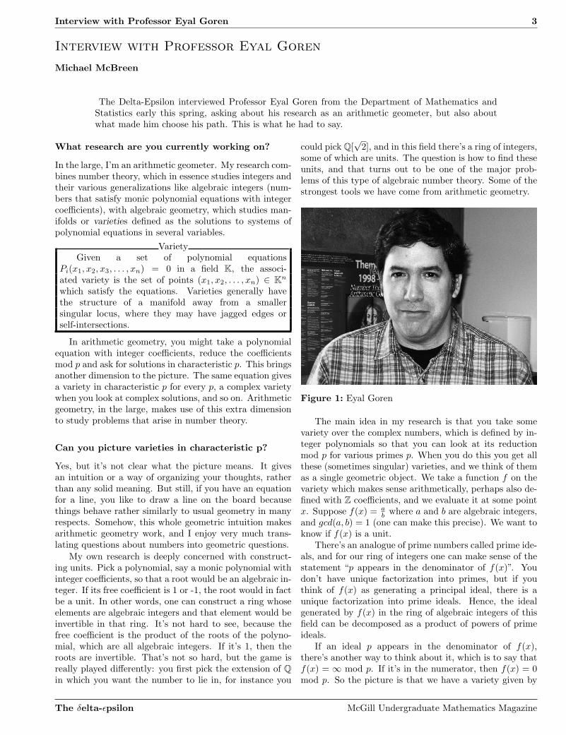
Figure 1: Eyal Goren
The main idea in my research is that you take somevariety over the complex numbers, which is defined by in-teger polynomials so that you can look at its reductionmod p for various primes p. When you do this you get allthese (sometimes singular) varieties, and we think of themas a single geometric object. We take a function f on thevariety which makes sense arithmetically, perhaps also de-fined with Z coefficients, and we evaluate it at some pointx. Suppose f(x) = a
b where a and b are algebraic integers,and gcd(a, b) = 1 (one can make this precise). We want toknow if f(x) is a unit.
There’s an analogue of prime numbers called prime ide-als, and for our ring of integers one can make sense of thestatement “p appears in the denominator of f(x)”. Youdon’t have unique factorization into primes, but if youthink of f(x) as generating a principal ideal, there is aunique factorization into prime ideals. Hence, the idealgenerated by f(x) in the ring of algebraic integers of thisfield can be decomposed as a product of powers of primeideals.
If an ideal p appears in the denominator of f(x),there’s another way to think about it, which is to say thatf(x) = ∞ mod p. If it’s in the numerator, then f(x) = 0mod p. So the picture is that we have a variety given by
The δelta-ǫpsilon McGill Undergraduate Mathematics Magazine
4 Interview with Professor Eyal Goren
polynomial equations, a point x on this variety (that is,a solution to those equations), and a function f on thevariety. And the function, the point and the variety canall be reduced mod p for most p. We define the 0-divisorof f roughly as the set of points where f(x) = 0, and the∞-divisor as the points where f(x) = ∞, and the state-ment that p is in the denominator of f(x) translates assaying that x mod p belongs to the ∞-divisor of f . Allthis works for general varieties and functions f , but themain idea here is to use a variety and a function whereeverything has an extra meaning. The varieties we are us-ing are parameter spaces or “moduli spaces”. The simplestexample is the variety that classifies elliptic curves up toisomorphism, i.e. whose points correspond to isomorphismclasses of elliptic curves.
Elliptic curvesAn elliptic curve is the set of solutions (x, y) to the
equation
y2 + a1xy + a3y = x3 + a2x2 + a4x + a6,
where we require that the resulting curve be nonsingular: if we write the equation as f(x, y) = 0,there is no point (x0, y0) such that d
dxf(x, y)|x0,y0and
ddy f(x, y)|x0,y0
are both zero. In C2, elliptic curves aretori.
You can look at a function on this space which vanishesexactly on the elliptic curves with some property - let’s callit “spin”. This is just a name, and there is no connectionto spin in physics. Take a point x without this property,i.e. such that f(x) 6= 0. To say that p appears in f(x)is to say that mod p, the elliptic curve has spin. That’snow a question about elliptic curves. It sounds like a lotof machinery to solve a simple-minded question, but thetruth is that we can almost never solve the simple questiondirectly. By cleverly choosing spaces, functions and points,you can translate the original question of whether f(x) isa unit into the question of whether the elliptic curve ac-quires a special property mod p, and these are questionswe can say much more about.
A lot of my research is concerned with the behavior ofelliptic curves and their higher dimensional generalizationswhen you reduce them mod p: seeing how various prop-erties of these varieties behave when you reduce them. Itturns out that those properties, when defined properly, areessentially geometric.
One interesting feature, and for many of us it’s a veryfrustrating feature, is that we almost never have equationsfor our moduli spaces. We know that they exist and arealgebraic varieties, but we can’t really describe them withequations. Everything goes through these translations: ev-ery point in the space has an extra meaning.
We talked about spaces which classify elliptic curves,and among these there are those that have some specialproperty. Similarly, you can have abelian varieties, whichare higher dimensional analogues of elliptic curves, andthey might have some interesting properties - part of the
game is to define such good properties. And then you lookat all abelian varieties with this property and you try toprove, for example, that they form a subvariety of the mod-uli space classifying all abelian varieties of this type. Allthis using pure thought, so to speak, never using equations:it would be horrible with equations, perhaps impossible.
The subvarieties that arise this way include those calledShimura varieties, and are very important in number the-ory and algebraic geometry. Therefore, one wants to studythem further. For example, one may try to study the lo-cal nature of some property, in the sense that you have anabelian variety and you ask if I slightly deform it, will thedeformation preserve this property. Usually the answer isno. You then ask yourself under what conditions will thedeformation preserve the property. And if you can findsuch conditions, that tells you about the local structure ofthe varieties you are defining.
These are very roundabout techniques, and definitelywhen one is first exposed to all this one should be very sus-picious as to whether the whole thing is worth the effort,but I think the answer is yes, we are proving stuff, andthe spaces we obtain are important for physics and otherapplications.
Prof. Goren now tells us about a different aspectof his research, certain cryptographic tools calledhash functions.
This part of my work is in collaboration with KristinLauter from Microsoft research. Amazingly, it relates tothe units we discussed earlier, but it would be too long toexplain the connection here.
Hash functions are critical tools in certain security pro-tocols used over the internet, for example in the digitalsignature protocols used in online transactions. From amathematical viewpoint, a hash function is a rather sim-ple object; it takes a bit string of arbitrary length and pro-duces a string of fixed length, say 32 bits. A very primitiveexample would be the following: if I wanted to check thatnobody is tampering with my hard drive while I’m awayfrom my office, I could use a function which takes the wholecontent of my hard drive and returns a 32 digit number.I would run this function before leaving the office and runit again when I come back, and if I get the same 32 digitnumber, it’s very likely no-one messed with the hard drivewhile I was gone.
For this to work, you need functions which are verysensitive to small changes. If someone hacks into his bankaccount and adds a single digit to his savings, you want todetect that. You also want it to be very hard for a personto know which changes to make to modify the value of thehash function in any given way.
Many of the currently used hash functions are quitesimple: you have this big potato, and you chop it up andfry it and so forth until it’s unrecognizable. You try todo something very complicated and aggressive to the dataand do it many times, and you hope it ends up properly
The δelta-ǫpsilon McGill Undergraduate Mathematics Magazine
Interview with Professor Eyal Goren 5
hashed. But it turns out these protocols aren’t as secureas people thought, so there’s a big search for good hashfunctions.
We propose to take this huge string of bits and use itas directions to walk on a graph. Imagine a graph whereeight edges go out from every vertex. The first part of thestring tells you which vertex to start on. Then you chopthe rest of the string into 3 bit pieces, and each 3-bit se-quence, which can encode 8 different possibilities, tells youwhich edge to move along next. Each vertex has a label,and the label of the end vertex is the output of the hashfunction.
You don’t want someone to be able to modify a few bitsof the input but still reach the same end vertex. You wanta graph where if you change even a single bit of input, youcould end up somewhere completely different. There arealso other cryptographic requirements that put additionalconditions on the process. So how do you construct a graphof this sort? It turns out that the best constructions thatwe know of come from number theory, and involve modularforms and elliptic curves, or abelian varieties, in character-istic p.
By using number theory to construct the graphs, we’reable to translate the security requirements of the hashfunctions into questions about elliptic curves, for exam-ple. In other words, we translate the problem of crackingthe hash function into a problem about elliptic curves. Youcan’t really prove that a Hash function is secure: you canonly show that the obvious attacks fail. In some sense, youplay the devil’s advocate by inventing methods of attackand showing that they fail. Since people have been think-ing about the relevant number theoretic problems for morethan a century now, we feel confident that the translatedproblem is truly hard, and this somehow justifies our faithin the security of the hash function.
You can also use these graphs to create pseudo-randomnumber generators, or to sample data sets. One of the bestways to sample of data is to do it randomly, but there’s aprice to pay for randomness, in running time or otherwise:it’s really very difficult to generate random numbers. Sofinding ways to mimic randomness is a big deal in com-puter science.
How did you get into mathematics?
It’s really a series of events. When I was about to turn six,I became very sick and I had to spend the whole summerin bed. My dad got me books in math, because he wasafraid I wouldn’t be able to catch up in class, but I endedup studying all this math which was quite hard for a sixyear-old. I really enjoyed just staying in bed and doingthose exercises.
Later, when I was ten, we learnt in school about divisi-bility properties: when is a number divisible by 3, by 5, by11 and so on. I was totally obsessed with finding a rule forseven, which is very tricky. I can’t really explain it, butthe problem appealed to me. I spent that summer at my
Grandparent’s place in Haifa, which is a harbor city in thenorth of Israel, in this little villa. I remember spendingthe hours before falling asleep thinking about this prob-lem, and eventually solving it, and that was a tremendousreward for me.
So what is the rule for divisibility by 7?
Actually, I’ve given it as an assignment in Algebra 1, soit’s on my course webpage
When I was in High school, I remember buying thosebooks of the Schaum series – because they were the cheap-est, so I could afford them. I think I liked then to calcu-late a lot, and see what the answer is. I also had the goodfortune to be in contact with a professor from the He-brew University, who gave me real math books and helpedme read them and understand them, so I was exposed tohigher mathematics, but I was never sure I wanted to domath. My main interest in high school was biology. I wasvery interested in immunology, the workings of the im-mune system, which is a truly fascinating subject. Musicwas another possible career choice.
Basically, I got to studying math in university by elimi-nation. Biology became a total mess at that time, becauseall the current theories about the immune system werediscovered to be false, and there were too many theoriescoming out, so I thought “let these people figure out firstwhat they want to say, and then we’ll see.” As for music,I played the piano for many years, and I realized the lifeof a performer was too difficult: very stressful, very com-petitive, and very few get to a position where they canactually play for an audience.
So I started university in math and physics, but afterone semester I got very irritated with the physicists, be-cause nothing was defined: what is mass? How do youknow that those are the forces working on a ladder? Andso forth. So I decided to transfer into math. Even then, Idid a lot of other things during my studies. For instance,I had a break of two years working in agriculture. I did dosome math during that period - I actually corresponded byletter with Ehud de Shalit from Hebrew University, whoeventually became my thesis supervisor.
What got me back to mathematics, and what keeps mewanting to do research, is in some sense the same thingthat had piqued my interest when I was five, or ten: Ireally wanted to understand why things were true, whatis the structure there - how do you tell, what’s the pat-tern. It comes from a place which is unmotivated by moresophisticated considerations.
How does it feel, when you suddenly go from apost-doc to a professor?
Actually, I think graduate school is the most exciting part.You have a lot of responsibilities as a professor, so in somesense graduate school is the time when you’re the mostcarefree, and it’s where your mind really expands. I re-
The δelta-ǫpsilon McGill Undergraduate Mathematics Magazine
6 Interview with Professor Eyal Goren
member, during my studies, encountering concepts that Ihad never thought of before, and it was very unsettling.
For instance, the first time I heard of the Banach-Tarskiparadox. You take a solid unit ball in R3, you divide it intofinitely many parts, and then using only rigid transforma-tions - no bending or anything like that - you can reassem-ble those parts into two solid unit balls. For me this wasvery unsettling, I remember being deeply troubled by thisphenomenon for weeks, because it shattered my intuitionand the way I understood the relevance of mathematics.
Another example is the notion of different cardinalitiesof infinite sets. When I was fourteen, I was babysitting myneighbor’s child. This neighbor had a degree in math, andone day he proved to me that there were the same numberof integers as squares, and that was a revolution for me. Iremember trying for weeks to check whether certain setsare the same size or not, and you could feel the mind phys-ically rewiring itself to digest these new phenomena. Asyou progress, you get more professional and there are lessand less instances like that, where you feel that a wholenew universe is being opened to you. Graduate school isa great time for that. There are other discoveries later on,
you discover your own theorems, but they’re very rarelyon the same fundamental level.
Any advice for undergraduates?
This is not just for undergraduates, this is universal advice.When people undertake a long term project, for instancegetting a degree or a PhD, very often they tend to for-get halfway why they’ve started it. They know they haveto finish it, but they can’t reconnect to the things thatprompted them to undertake this project to begin with.You see this phenomenon when classes are cancelled andeveryone is happy, which is pretty ironic, because you cameto university to learn this stuff, you’ve made that choice.So it’s good to try and reconnect to the reasons that gotyou to university, or made you go into the Ph.D. programand so on. This applies especially in math - I think peo-ple choose math for the same kind of reasons that I wasdescribing earlier, and I think it’s very important to re-connect to this desire to know, to learn more about thesepatterns, and to appreciate their beauty.
Jokes
A mathematician, a physicist, and an engineer are all given identical rubber balls and told to find the volume. Theyare given anything they want to measure it, and have all the time they need. The mathematician pulls out a measuringtape and records the circumference. He then divides by two times pi to get the radius, cubes that, multiplies by piagain, and then multiplies by four-thirds and thereby calculates the volume. The physicist gets a bucket of water,places 1.00000 gallons of water in the bucket, drops in the ball, and measures the displacement to six significant figures.And the engineer? He writes down the serial number of the ball, and looks it up. ¤
An engineer, a physist and a mathematician are sent to a desolated jail. The engineer is sent in first, alone, withnothing but a can containing his only potential source of food. After a few minutes, he looks into his pocket, findssome trash and make a can opener out of it. He then eats almost all the food and use the rest and the can to make asmall bomb to break the wall of his cell. He escapes, retires at the age of 55 to go travel around the world on a boat,and lives happily ever after.The physists is then sent in and, again, his only hope resides in his can of food. After a few hours, he takes a rockand writes on the ground. He then computes the exact angle and force at which he needs to throw his can to destroyboth the can and the wall. He eats the food, escapes and starts a new ground-breaking theory in which everything isrepresented as tiny 24 dimensional cans.The mathematician is then sent in the prison. After a week, the guardians come. They find him dead in his ownblood, lying face down in the corner of the cell. In the exact middle, the can lay perfectly still, and closed. Aroundit, an elegant drawing accompagnies a beautiful proof of the sphere packing problem – written in blood. Next to themathematician, the guardians find, and clean away in their ignorance, some text: “Theorem. If I don’t open the can,I will die. Proof. Suppose not.” ¤
The δelta-ǫpsilon McGill Undergraduate Mathematics Magazine

On Primes in Arithmetic Progressions 7
On Primes in Arithmetic Progressions
Vincent Quenneville-Belair
Dirichlet’s theorem is proved using the Riemann Zeta Function and similar Dirichlet series basedon characters. Indeed, the similar series satisfy an identity that will be used to derive an asymptotefor the sum of the reciprocals of primes in some congruence class, under the condition that theyare bounded away from zero.
Theorem (Dirichlet’s Theorem). An arithmetic progres-sion a + nm∞n=0 where a, n,m ∈ Z contains infinitelymany primes when gcd(a,m) = 1.
Introduction
Dirichlet proved the infinitude of primes in arithmetic pro-gressions in 1837 using ideas from Euler’s proof about theinfinite number of primes – a task so great that it is claimedto be the crowning achievement of the XIXth century1 innumber theory. The theorem equivalently states that thereexist infinitely many primes congruent to a mod m when aand m are coprime. The proof starts by noting that ζ(s),the Riemann Zeta Function, has a simple pole at s = 1and continues with the definition of similar series with thekey property that they are bounded away from zero. Thatis a major point: showing that these series are not zeroas s approaches 1 from the right. A survey of characters,examples of periodic functions from the integers to themultiplicative group of the complex numbers, will be nec-essary in defining these Dirichlet L Series. Euler’s geniuscomes into play when finding a factorization of all these se-ries and deriving from them an asymptotic behaviour forsums of primes. It is worth noting before beginning thefollowing simple result: an arithmetic progression containsat most one prime when gcd(a,m) > 1.
Riemann Zeta Function
The Riemann Zeta Function has very special propertieslinked to extremely deep topics in mathematics – such asthe Riemann Hypothesis, which claims that all the non-trivial zeros are on the ℜ(s) = 1/2 line. The journey intothe proofs of Dirichlet’s Theorem starts with the study ofthe Riemann Zeta Function and similar series. It is impor-tant to know that the next definition only makes sense forℜ(s) > 1.
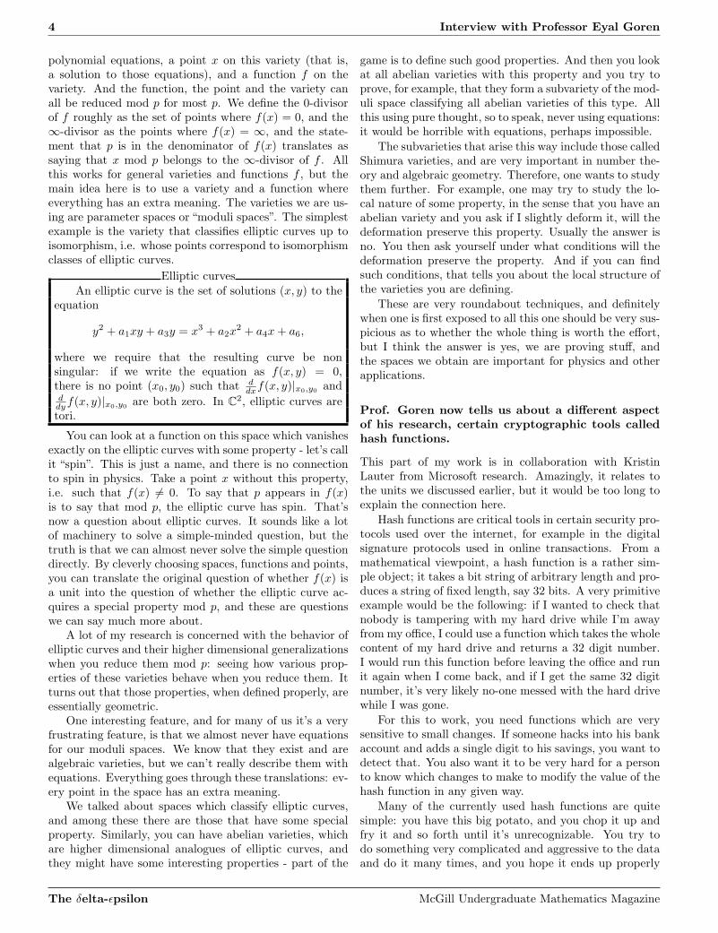
Definition 1. The Riemann Zeta Function, denoted ζ(s),is defined to be the following series for ℜ(s) > 1: [2]
ζ(s) =
∞∑
n=1
1
ns.
0
0.5
1
1.5
2
2.5
3
1 10 100
Figure 1: ζ(s) up to roughly 30 terms in the series on1 < s < 100.
Interestingly, ζ(s) can be extended uniquely to an ana-lytic function with a simple pole at s = 1. The uniquenessfollows from an important result in complex analysis stat-ing that if two functions f and g are analytic on a domainD and that there exists a sequence zn of points in D ac-cumulating at ω in D such that f(zn) = g(zn) then f = geverywhere in D [3].
Property 1. ζ(s) is absolutely convergent for ℜ(s) > 1.
This will follow from the proof of property 2, but theadaptation of the proof is left to the reader.
A function has a pole of order N at an isolated pointz0 if it diverges to infinity if the limit of (z − z0)
Nf(z) asz approaches the singular point z0 is neither zero nor ∞.
Property 2. ζ(s) has a simple pole at s = 1
Proof. Using the integral test for series,∫ x+1
1
dt
ts≤
x∑
n=1
1
ns≤ 1 +
∫ x
1
dt
ts
−1
s − 1
1
(x + 1)s−1≤
x∑
n=1
1
ns− 1
s − 1≤ 1 − 1
s − 1
1
xs−1.
Fixing s > 1 and letting x going to infinity,
0 ≤ ζ(s) − 1
s − 1≤ 1.
The result follows from the fact that lims→1+ ζ(s) = ∞but lims→1+ ζ(s)(s − 1) = 1. ¤
1Citation from a number theory lecture on March 2nd 2007 by Professor Henri Darmon.
The δelta-ǫpsilon McGill Undergraduate Mathematics Magazine

8 On Primes in Arithmetic Progressions
0
0.5
1
1 2 3 4 5 6 7 8
Figure 2: Approximating 1/x by sums.
Characters
Definition 2. A character χ modulo m (where m ≥ 1) isa homomorphism from (Z/mZ)∗ to C∗. It is extended toall Z by setting χ(a) = 0 when a is not coprime with m.[2]
From now on, α(n) is the order of n in (Z/mZ)∗, i.e.the smallest integer strictly greater than 1 with nα(n) ≡ 1(mod m). Note that α(n)|φ(m) by Euler’s theorem, whereφ(m) is the Euler-Phi function (φ(p) = p − 1 when p is aprime).
These characters χ(n) modulo m can be viewed as mul-tiplicative functions in the strict sense on Z, which haveperiod m, have image in C∗, are zero when n is not co-prime to m and take values among the α(n)th-roots ofunity. Furthermore, it is an important fact that there areφ(m) distinct characters for a fixed modulus m. Indeed,the group formed by the characters is abstractly isomor-phic to (Z/mZ)∗ which has φ(m) elements. [1, 2] Fromnow on, the modulus m is fixed.
Lemma 1. If χ = 1,∑
a χ(a) = φ(m), or otherwise zero.[2]
Proof. For χ = 1, the sum counts the number of elementsin (Z/mZ)∗ and is hence φ(m). If χ 6= 1, consider multi-plying by χ(b) 6= 1, knowing that b(Z/mZ)∗ = (Z/mZ)∗:
χ(b)∑
a
χ(a) =∑
a
χ(ab) =∑
a
χ(a).
Thus, (χ(b)−1)∑
a χ(a) = 0 which implies that∑
a χ(a) =0. ¤
The previous proof can be adapted to obtain the nextlemma.
Lemma 2. If a ≡ 1 (mod m),∑
χ χ(a) is either φ(m) or0. [2]
Proof. If a ≡ 1 (mod m), χ(a) = 1 and thus the sum iscounting the number of characters. If a 6≡ 1 (mod m), onetakes χ′(a) 6= 1 and
∑
χ
χ(a) =∑
χ
χ(a)χ′(a) = χ′(a)∑
χ
χ(a)
which implies as in lemma 1 that the sum is zero. Theprevious equation uses the fact that χ(a) takes values inthe α(a)th-roots of unity and that multiplying by one ofthem simply permutes them: their sum is thus the same.
¤
Dirichlet L Functions
With characters in hand, one can define the Dirichlet Lfunctions.
Definition 3. A Dirichlet L function [2] is a series
L(s, χ) =
∞∑
n=1
χ(n)/ns.
where χ(n) is a character modulo m.
Now, these series are absolutely convergent for ℜ(s) >1 from property 1 (their absolute value is bounded by theabsolute value of ζ(s)). Furthermore, one can use the nextproperty to show that the series converges uniformly forℜ(s) ≥ δ > 0 if χ 6= 1, which implies that L(s, χ) is con-tinuous for ℜ(s) > 0. The proof will be omitted: however,an interested reader can look for Abel’s sum in referencessuch as [2].
Property 3. For χ 6= 1, L(s, χ) converges (maybe notabsolutely) for ℜ(s) > 0. [2]
Property 4. The Dirichlet L function can be factored ina manner similar to Euler’s identity:
L(s, χ) =∏
p
(
1 − χ(p)
ps
)−1
.
Proof. With p denoting a prime from here onwards and pr
the greatest prime smaller than x,
∏
p<x
(
1 − χ(p)
ps
)−1
=∏
p<x
(
1 +χ(p)
ps+
χ(p)2
p2s+ ...
)
= lime→∞
∑
0≤e1,e2,...,er≤e
χ(pe1
1 pe2
2 ...perr )
(pe1
1 pe2
2 ...perr )
s
=∑
n x-smooth
χ(n)
ns
where a number n ∈ N is x-smooth if all its prime fac-tors are strictly smaller than x. The result is obtained byletting x going to infinity. ¤
The δelta-ǫpsilon McGill Undergraduate Mathematics Magazine
On Primes in Arithmetic Progressions 9
Using exactly the same method, one obtains the fac-torization of ζ(s). Remark also that L(s, 1) is similar toζ(s), in fact,
L(s, 1) =∏
p∤m
(
1 − 1
ps
)−1
= ζ(s)∏
p|m
(
1 − 1
ps
)
. (1)
Asymptotes concerning Primes
By taking the logarithm of both sides in property 4, weget
log L(s, χ) = − log∏
p
(
1 − χ(p)
ps
)
=∑
p
∑
n∈Z+
χ(pn)
npns. (2)
Again, replacing χ by 1 yields the result for ζ(s):
log ζ(s) =∑
p
p−s +∑
p
∞∑
n=2
1
npns
=∑
p
p−s + O(1), (3)
with the left side diverging as s approaches 1. It followsthat there are infinitely many primes and that the sum oftheir reciprocal diverges. Turning to equation 2 and divid-ing by χ(a) 6= 0, summing over all characters and applyinglemma 2,
∑
χ
χ(a)−1 log L(s, χ)
=∑
p
∑
n∈Z+
pn≡a(m)
n−1p−nsφ(m)
= φ(m)∑
p≡a(m)
p−s + φ(m)∑
p
∞∑
n=2pn≡a(m)
n−1p−ns
= φ(m)∑
p≡a(m)
p−s + O(1). (4)
If we can show that for χ 6= 1, L(s, χ) is non-zero ass → 1+, then the proof would be done: it would followthat the left hand side diverges, implying that there areinfinitely many primes congruent to a (mod m). [1]
Away from Zero
Naturally, it remains to prove that the Dirichlet L seriesare not zero as s → 1+.
Lemma 3. Let n 6≡ 0 (mod m), g(n) = φ(m)/α(n) andT = p−s. Then
∏
χ
(1 − χ(n)T ) = (1 − Tα(n))g(n),
where α(n) is the order of n in (Z/mZ)∗. [2]
Proof. First, consider W , the set of α(n)th-roots of unity.One has
∏
w∈W
(1 − wT ) = 1 −∑
w∈W
wT +∑
wi 6=wj∈W
wiwjT2
− ... + (−1)nTα(n)
= 1 − Tα(n).
Recall that the sum of all the roots of unity yields zero.The result follows since there are g(n) character modulom such that χ(n) = w. ¤
Having lemma 3 in hand (with T = p−s), it is nowpossible to factorize ζm(s) using equation 4 for ℜ(s) > 1where convergence is clear [2],
ζm(s) =∏
χ
L(s, χ) =∏
χ
∏
p
(
1 − χ(p)
ps
)−1
=∏
p∤m
(1 − p−sα(p))−g(p). (5)
Property 5. L(1, χ) 6= 0 when χ 6= 1. [2]
Proof. Suppose L(1, χ) = 0 for some χ. It would implythat ζm(s) is convergent for ℜ(s) > 0 since, as mentionedbefore, the simple pole of L(s, 1) at s = 1 would be re-moved by the zero of L(s, χ). Now, the right hand side ofequation 5 is
ζm(s) =∏
p∤m
(1 + p−α(p)s + p−2α(p)s + ...)g(p)
≥∏
p∤m
(1 + p−φ(m)s + p−2φ(m)s + ...)
≥∑
p∤m
1
pφ(m)s
but this last series goes to infinity as s → 1/φ(m) since thesum of the reciprocal of the primes diverges. This contra-dicts the convergence of ζm(s) and, hence, all L(1, χ) arenon-zero. ¤
Conclusion
Now, the left side of equations 4 diverges since, for χ 6= 1,L(s, χ) is bounded away from zero and so log(L(s, χ)) isbounded. Hence, the right side must diverge, becauseL(s, χ1) diverges, and thus so does the sum of the recipro-cal of the primes congruent to a modulo m. Done!
The author thanks professor Henri Darmon for hisguidance during the writing of this article.
References
[1] Harold Davenport. Multiplicative Number Theory.Springer, third edition, 2000.
[2] Jean-Pierre Serre. A Course in Arithmetic.Springer, 1973.
[3] David Wunsch, A. Complex Variables with Applica-tions. Pearson Education, third edition, 2005.
The δelta-ǫpsilon McGill Undergraduate Mathematics Magazine

10 Object Detection Using Feature Selection and a Classifier Cascade
Object Detection Using Feature Selection and a Classifier Cascade
Rishi Rajalingham
To construct an object-detector, one must provide a classifier model with training data from whichit will “learn” what distinguishes the object class. Commonly, the training data in question is alarge set of labeled images of class and non-class objects, and the distinguishing features are edgesextracted from these images. The set of all edges in the training data, or feature space, is large,and hence training a classifier is time-consuming. Furthermore, once trained, classification may becrude or slow in conventional methods. This paper will briefly describe the proposition to reducethe complete set of features, using Francois Fleuret’s conditional mutual information maximization(CMIM) algorithm, to a few most informative features; hence, the training time is considerablyreduced. Moreover, the classifier is trained as a cascade of weak classifiers, rejecting non-classimages quickly, as per Viola and Jones [1] , thus reducing classification time as well.
Conditional Mutual Information Maxi-
mization
In [2], Fleuret introduces the probabilistic notion of mu-tual information, specifically conditional mutual informa-tion maximization (CMIM), to the field of object detec-tion. The purpose of the CMIM algorithm is ultimatelyto select, from a given feature space, the small numberof features that are deemed most informative and hencebest represent a class of objects. It follows intuitively thatclassifying using this reduced set of features is far moreefficient than using the complete set.
To understand CMIM, first recall from information the-ory the concept of entropy (H) of a variable: H(U) rep-resents the uncertainty of U . Moreover, the conditionalentropy of a variable, H(U |V ) , represents the uncertaintyof U when V is known. (Thus it is trivial that, if U is afunction of V alone, then H(U |V ) = 0, and if U and Vare independent, then H(U |V ) = H(U) .) Using this, itis now possible to express conditional mutual information(I) as:
I(U ;V |W ) = H(U |W ) − H(U |W,V ).
The value I(U ;V |W ) gives an idea of the informationshared between U and V , given W . Within the objectdetection application, U must be understood as a class ofobjects, V as a feature about to be selected (or rejected),and W as the set of features already selected.
Thus, if the new feature V carries no or little new in-formation on the class, given some pre-selected features,then both conditional entropy terms are equal, or similar,and the conditional mutual information is zero, or small.Likewise, if the new feature V brings forth much new in-formation of the class U , which is what we seek, the con-ditional mutual information will be large. The reason forthe term ‘maximization’ now becomes clear.
To further tie this to the present application, letX1, . . . ,XN be the N features in the complete set. Forcommon object detection problems, the variable N is in theorder of tens of thousands. Likewise, let XV (1), . . . ,XV (K)
be the K features in the reduced set, where K is in the
order of tens. XV (1), . . . ,XV (K) can be obtained by it-erating over the complete set: first selecting the most in-formative feature XV (1), and subsequently selecting, andadding to the reduced set, the feature XV (i) for which theconditional mutual information is largest. For the com-plete algorithm or implemented code, refer to [2].
The advantages of using this reduced set of features lienot only in efficiency in computation power and time, butalso in theoretical performance. Indeed, by using fewerfeatures per classifier, the phenomenon of “overfitting” isavoided. Overfitting occurs when too many parameters,or in this case, features, relative to the training data need-lessly increases the complexity of the classifier model, pos-sibly resulting in a very poor classifier.
Features and Filters
Due to its computational complexity, and consequently,large computation time, the CMIM algorithm necessitatesthe use of very crude features that take limited values.This is best done by using binary features, where a valueof 1 indicates the presence of a specific edge, and 0, theabsence. Features are obtained by running filters over im-ages. The filters used in this approach are similar to theedge fragment detectors used in [3], and are called “crudeedge detectors”. Briefly, they return true (or binary 1) ifthe contrast between pixels across the supposed edge isgreater than the contrast between pixels along the edge.
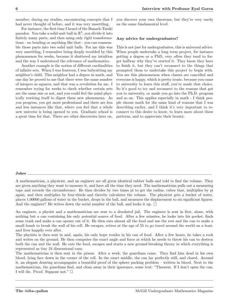
Running these filters of all eight orientations (see Fig-ure 1), in neighborhoods of size varying between 1 and 7pixels, at every pixel location of a training image of size24×24, we obtain 20×20×8×7 = 22400 features in total.
Weak Classifier Models
The classifier models implemented are linear classifiers;given any image from which N input features are ex-tracted, or alternatively given any feature vector ~x =(x1, . . . , xN ), the class is determined using:
f(~x) = sgn (〈~x, ~ω〉 + b) ,
The δelta-ǫpsilon McGill Undergraduate Mathematics Magazine

Object Detection Using Feature Selection and a Classifier Cascade 11
Figure 1: The crude edge detectors (top) return true ifthe contrast between the two pixels shown in solid dotsis greater than the contrast of neighbouring pixels, shownwith white circles. The detectors of four directions mapthe dark disk on the left to the corresponding edge maps(bottom).
for bias b and weight vector ~ω = (ω1, . . . , ωN ) computedin the training phase, and standard inner product 〈~x, ~ω〉. The Signum (sgn) function returns the sign of its argu-ment, and hence, the class of the image (positive or nega-tive).
This concept may be understood geometrically by vi-sualizing ~x as a point in N -space, while Π(~u) = ~u · ~ω + bis the equation for an (N − 1)-flat, or hyperplane, havingnormal vector ~ω and constant term b. It should be clearthat the hyperplane Π cuts the space in two, thus deter-mining the class of any image ~x by its coordinates. Whatremains is to determine the particular Π for each classifier,or equivalently to determine its ~ω and b. The following aremethods for determining the weights and bias.
Perceptron
The classical Perceptron (see [4], [5]) provides an iterativemethod, the Perceptron learning algorithm, to computethe weight vector. The vector, ~ω, is initialized and itera-tively corrected in the training process. If a training ex-ample is incorrectly classified, its feature vector is addedor subtracted, depending on its true class, to the weightvector. This process is known to converge for linearly sep-arable training sets.
Naive Bayesian Classifier
The naive Bayesian classifier classifies by comparing prob-abilities with a simple inequality. Let ~x = (x1, x2, . . . , xN )be the feature vector of an image, and Y (1 for positive, 0for negative), its class label. Then
f(x) =
1,P (Y = 1|X1 = x1, . . . ,XN = xN )
> P (Y = 0|X1 = x1, . . . ,XN = xN );
0, else.
or equivalently,
f(~x) = sgn
logP (Y = 1|X1 = x1, . . . ,XN = xN )
P (Y = 0|X1 = x1, . . . ,XN = xN )
.
Now, recall from statistics that for events A,B, Bayes’Theorem states that
P (A|B) =P (B|A) · P (A)
P (B).
Hence, assuming the Xi’s are conditionally independent (anaive assumption), and applying Bayes’ Theorem, we have
f(~x)
= sgn
log
∏Nk=1 P (Xk = xk|Y = 1)
∏Nk=1 P (Xk = xk|Y = 0)
+ logP (Y = 1)
P (Y = 0)
= sgn
N∑
k=1
logP (Xk = xk|Y = 1)
P (Xk = xk|Y = 0)+ log
P (Y = 1)
P (Y = 0)
Thus, we have arrived at the linear form f(~x) = sgn(~x ·~ω + b), with
ωk = logP (Xk = 1|Y = 1)P (Xk = 0|Y = 0)
P (Xk = 1|Y = 0)P (Xk = 0|Y = 1).
The Bayesian weight computation required no iteration(and thus cannot fail to converge), while still outdoing thePerceptron in both speed and accuracy. Despite the naiveassumption, experiments show that the Bayesian classifierresults in lower error rates when dealing with ‘real life’cases.
Bias
Assuming that the training set is well representative of theclasses in question, one should see in the distribution of theweighted sum of inputs, two quasi-distinct regions repre-senting the positive and negatives, respectively. It sufficesthen, for prescribed error rates, to estimate empirically athreshold value θ that best separates the classes. The biasb is then simply the negative of θ.
Strong Classifier: An Attentional Cascade
Given the classifier models, we may now string togetherseveral such weak classifiers to construct a strong one. The“attentional cascade” of Viola and Jones [1] does just this,and provides a way to achieve high detection rates whiledrastically decreasing detection time. The principal as-sumption is that, in any given image, the vast majority ofobjects will be negatives. In the specific case of face de-tection, this is known to be a well-founded assumption, asimages seldom contain more than a dozen distinct faces,while the number of non-faces is generally on the order oftens of thousands.
Implementing an attentional cascade means construct-ing a decision tree. The cascading method discussed in thispaper involves training each weak classifier sequentiallyusing an increasing number of inputs until the error con-straints are satisfied by that particular weak classifier. Theconstraints determining the characteristics of the strongclassifier are on the true-positive and false-positive rates.The terms true-positive, false-positive, true-negative, andfalse-negative make reference to whether the classificationwas correct (true/correct or false/incorrect), and the clas-sification return value (positive image or negative image).For example, in the case of a face detector, a misclassifiedface image is a false-negative.
The δelta-ǫpsilon McGill Undergraduate Mathematics Magazine
12 Object Detection Using Feature Selection and a Classifier Cascade
Table 1: Perceptron learning algorithm.• Given a training set of m labeled images: Dm = ( ~x1, y1), ( ~x2, y2), . . . , ( ~xm, ym), where the ~xi
is the feature vector for the i-th training image and y its corresponding label• Given weights vector ~ω• For each (~xi, y) pair in Dm
Initialize weights ω(j) ← 0 Do until classifier converges or 5000 iterations:
· Compute ∂ =
1, if ~xi · ~w ≥ 0;0, else.
· Update ω(j) ← ω(j) + (∂ − y)xi(j).
Table 2: Cascade training algorithm.• Given a set of labeled training images• Given an array of features for each image (output from Fleuret’s CMIM algorithm [2])• Initialize number of inputs to two (n ← 2)• Do until all the features have been used
Train weak classifier i Evaluate classification error on training set If TP-rate > true positive constraint and FP-rate < false positive constraint
· Move to next weak classifier (i ← i + 1)· Reset number of inputs (n ← 2)
Else· Increase number of inputs (n ← n + 1)
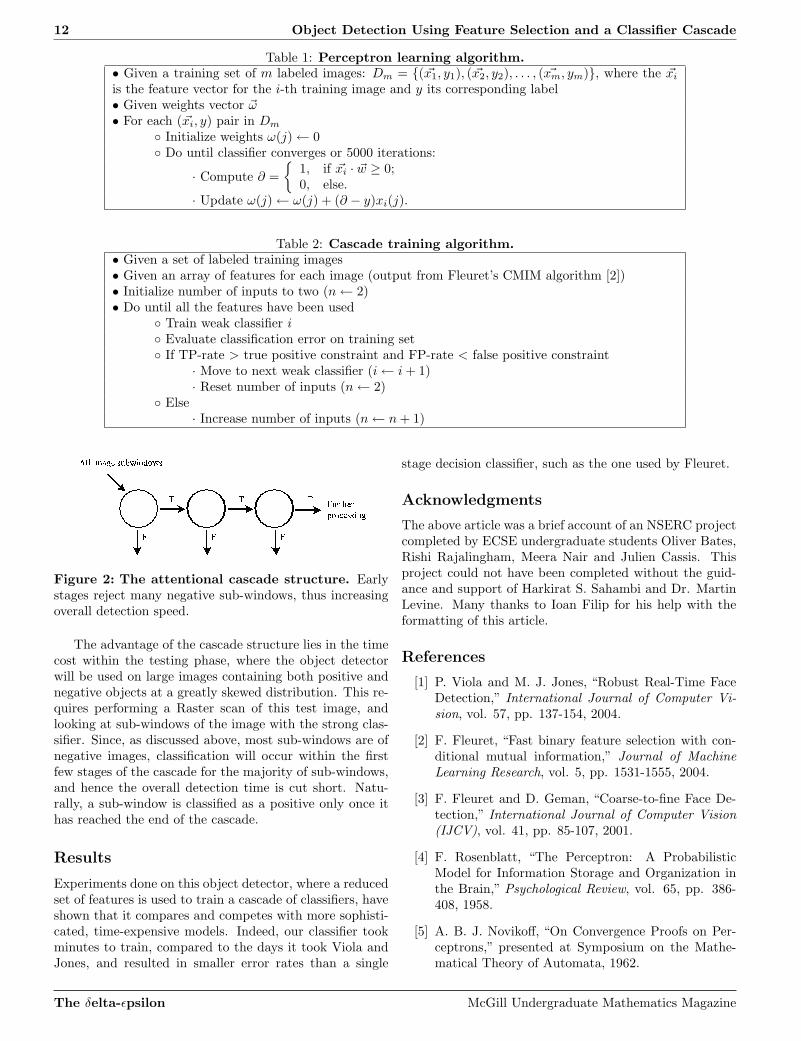
Figure 2: The attentional cascade structure. Earlystages reject many negative sub-windows, thus increasingoverall detection speed.
The advantage of the cascade structure lies in the timecost within the testing phase, where the object detectorwill be used on large images containing both positive andnegative objects at a greatly skewed distribution. This re-quires performing a Raster scan of this test image, andlooking at sub-windows of the image with the strong clas-sifier. Since, as discussed above, most sub-windows are ofnegative images, classification will occur within the firstfew stages of the cascade for the majority of sub-windows,and hence the overall detection time is cut short. Natu-rally, a sub-window is classified as a positive only once ithas reached the end of the cascade.
Results
Experiments done on this object detector, where a reducedset of features is used to train a cascade of classifiers, haveshown that it compares and competes with more sophisti-cated, time-expensive models. Indeed, our classifier tookminutes to train, compared to the days it took Viola andJones, and resulted in smaller error rates than a single
stage decision classifier, such as the one used by Fleuret.
Acknowledgments
The above article was a brief account of an NSERC projectcompleted by ECSE undergraduate students Oliver Bates,Rishi Rajalingham, Meera Nair and Julien Cassis. Thisproject could not have been completed without the guid-ance and support of Harkirat S. Sahambi and Dr. MartinLevine. Many thanks to Ioan Filip for his help with theformatting of this article.
References
[1] P. Viola and M. J. Jones, “Robust Real-Time FaceDetection,” International Journal of Computer Vi-sion, vol. 57, pp. 137-154, 2004.
[2] F. Fleuret, “Fast binary feature selection with con-ditional mutual information,” Journal of MachineLearning Research, vol. 5, pp. 1531-1555, 2004.
[3] F. Fleuret and D. Geman, “Coarse-to-fine Face De-tection,” International Journal of Computer Vision(IJCV), vol. 41, pp. 85-107, 2001.
[4] F. Rosenblatt, “The Perceptron: A ProbabilisticModel for Information Storage and Organization inthe Brain,” Psychological Review, vol. 65, pp. 386-408, 1958.
[5] A. B. J. Novikoff, “On Convergence Proofs on Per-ceptrons,” presented at Symposium on the Mathe-matical Theory of Automata, 1962.
The δelta-ǫpsilon McGill Undergraduate Mathematics Magazine

Optimizing Efficiency of a Geothermal Air Conditioner 13
Optimizing Efficiency of a Geothermal Air Conditioner
Alexandra Ortan and Vincent Quenneville-Belair
The underlying principle of a geothermal air-conditioning is to extract heat from the soil by runningwater through a series of pipes in the ground. However, since the installation costs of such a heatpump is very high, its configuration must be designed in such a way as to minimize them. Therelationship between power output and controlable parameters such as pipe radius and length isinvestigated to this end. A derivation of the temperature profile of the soil is done in order totake advantage of the greatest temperature difference. Two models are used for the water runningthrough the pipes: plug flow and Poisseuille flow, which were then used to predict the length ofpipe necessary.
Problem Description
A geothermal heating system takes advantage of the factthat the temperature of the soil fluctuates slower than thatof air, and in fact is almost stable at a certain depth. A se-ries of pipes is buried in the ground following different con-figurations, and water is circulated through them. Thusthe water either heats up or cools down depending on theseason. A heat exchanger installed in the house then usesthis water to either heat or cool the house and the waterre-enters the cycle.
The configuration of the pipes through the ground canbe either vertical or horizontal. As shown in the figuresopposite, the pipes can be streched out or coiled together.A variant of the system is to put run the pipes through apond of water, for better conductivity. A detailed analysisof each of them however could reveal the main differencesand thus allow for better choices of the most appropriateconfiguration.
The efficiency of such a system relies on how much heatcan be exchanged with the soil. Generally speaking, thelonger the pipe carrying water through the ground, thebetter the heat exchange. However, other factors, such asflow rate, pipe radius and geometry of the pipe are alsoto be considered in calculating the heat transfer occurringbetween water and soil.
Soil Temperature Profile
The premise of the geothermal heating system is that thesoil remains at almost constant temperature at a certaindepth. In order to take the best advantage of that, oneneeds to know exactly how the soil responds to the sea-sonal temperature changes in the air and calculate thatdepth.
The variation of the temperature in function of thedepth in the soil can be set up as a partial differentialequation [1]. Indeed, it can be assumed that Θ(x, t), thetemperature in function of the depth and of the time, re-spects the heat diffusion equation:
Θt = αΘxx,
where α is the thermal diffusivity of the soil. The seasonalvariation of the soil’s surface temperature yields a periodic
boundary condition:
Θ(0, t) = TA + ∆Teiσt,
where TA is the average temperature throughout the yearand σ−1 is proportional to a month. Now, a trial func-tion to transform the PDE in an ODE can be used:Θ(x, t) = TA + AeiσtW (x). It then follows that
W ′′(x) =iσ
αW (x)
with W (0) = 1 and limx→∞ W (x) = 0. Trying thenW (x) = emx gives that m = ±
√
σ2α (1 + i). Since W (x)
decays with x increasing, the negative value of m must beused. Finally, the result lies in the real part of Θ(x, t):
T (x, t) = ℜΘ(x, t)
= TA + e−√
σ2α x cos
(
−√
σ
2αx + σt
)
. (1)
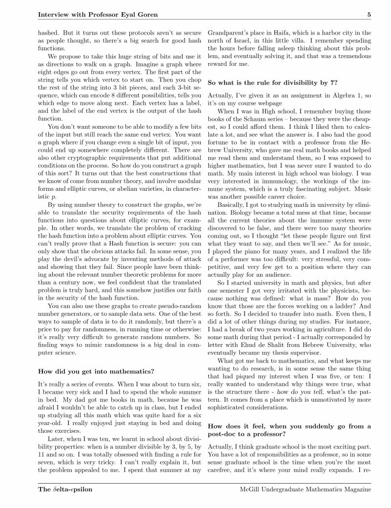
Using appropriate values for the constants gives thatthe ground temperature is almost uniformly 13C below2.5 m and that there is a temperature inversion at roughly1.5 m.
Winter Summer
Depth
Temperature
Ground
Air
Figure 1: Temperature profile in C of the ground forboth summer and winter as a function of the depth.
Plug Flow
A typical annual household’s energy consumption is about75 MBTU or around 80 MJ. Assuming water enters thesystem at 3C and heats up to the temperature of the soil,
The δelta-ǫpsilon McGill Undergraduate Mathematics Magazine

14 Optimizing Efficiency of a Geothermal Air Conditioner
that is 13C, a volumetric flow of 30 L/min would be re-quired to power the house. In a typical 1 cm pipes, thatmeans a flow rate of roughly 2 m/s.
Under the assumption that the soil remains at a con-stant temperature Ta and that the pipe is straight, it ispossible to find an equation for the power gained by a vol-ume element. First, using the relationship between energyand heat capacity, one has
P = ρw∆V cpw∆T
∆t(2)
for a change of temperature ∆T in a time ∆t of a volumeelement ∆V of water, and where ρw is the density of wa-ter and cpw is its thermal capacity. Now, the heat inputmust be related to the heat φ0 transferred from the soilto the pipe and the heat leaving the volume element byconvection φ1:
Φ = φ0 − φ1,
where φ0 = −hS(T − Ta) and φ1 = ρwAucpw∆T , with Sbeing the surface area of a volume element, A the cross-sectional area of the pipe and u the velocity of water inthe pipe and h the heat transfer coefficient.
Thus the governing equation for the temperature in thevolume element is:
ρw∆V cpw∆T
∆t+ ρwAu∆Tcpw
= −hS(T − Ta). (3)
In order to avoid references to a unit system, the equationshould be non-dimensionalized. Note that ∆V = A∆x =πR2∆x and that S = 2πR∆x, with R being the radius ofthe pipe. Taking the limit in which ∆x and ∆t go to 0,
ρwRcpwTt(x, t) + ρwRuTx(x, t)cpw
= −2h(T (x, t) − Ta) (4)
with boundary condition being T (0, t) = T1 and the initialcondition T (x, 0) = Ta, on can define x = x
R , T = TTa
,
t = 2hρRcpw
t and ǫ =ρcpw
2h u. The equation now becomes
Tt + ǫTx = 1 − T (5)
with boundary conditions T (0, t) = T1
Taand T (x, 0) = 1.
Solving for the steady state of the previous equation,and dropping the tilas for convenience,
T (x) = (T1 − Ta) e−x/ǫ + Ta.
Using this equation, it is possible to obtain the length ofthe pipe (as a function of radius, flow rate and initial tem-perature) needed by the water to reach a given tempera-ture T2, by solving for L in T (L) = T2
Ta:
L =Qρwcpw
2πRhln
(
T2 − Ta
Ta − T1
)
where Q = πR2u is the volumetric flow rate. Note thatthe length is dependent on h which can vary by up to anorder of magnitude, depending on the type of ground.
If u(t) = 0 in equation 4, it is possible to solve forT (x, t) since
Tt(x, t)
T (x, t) − Ta=
−2h
Rcpρ.
Integrating with respect to t yields
T = C(x) exp
( −2h
Rcpρt
)
+ Ta
where C(x) is a function determined by the initial condi-tion.
0
2
4
6
8
10
L
2 4 6 8 10 12 14 16 18 20
R
Figure 2: Expected pipe length in meters as a functionof the radius of the pipe using plug flow. The lowervalues seem to be too large to be practical. The topcurve uses h = 55W/Km
2, whereas the bottom curve uses
h = 675W/Km2.
Poiseuille Flow
A model refinement can be implemented by taking into ac-count non-uniform velocity profile in the pipe. Assumingu = u(r) with Poiseuille flow yields:
u = −∆P
4µ
(
R2 − r2)
,
where ∆P is change of pressure (assumed to be constantand negative) of the fluid. Now, the flow rate is
Q = 2π
∫ R
0
urdr
and the new energy equation
ρwcpwT t +Qρwcpw
πR2T x
= kwT xx − 2h
R
(
T − Ta
)
(6)
where T (x, t) was replaced by its average value over time,T (x, t).
The δelta-ǫpsilon McGill Undergraduate Mathematics Magazine
Optimizing Efficiency of a Geothermal Air Conditioner 15
Non-dimensionalizing gives
Pe
BiTt =
1
BiTxx + 1 − T ,
from which the steady-state temperature distribution is
T (x) = (T1 − Ta) eBiPe
x + Ta.
Thus to heat the water to T2, the length of the pipe mustbe
L = Rln
(
T2−Ta
T1−Ta
)
Pe −√
P 2e + 2Bi
0
0.2
0.4
0.6
0.8
1
L
2 4 6 8 10 12 14 16 18 20
R
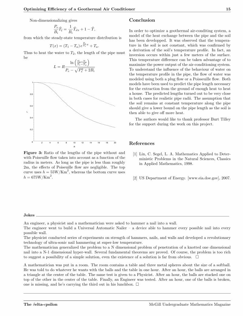
Figure 3: Ratio of the lengths of the pipe without andwith Poiseuille flow taken into account as a function of theradius in meters. As long as the pipe is less than roughly2m, the effects of Poiseuille flow are negligible. The topcurve uses h = 55W/Km
2, whereas the bottom curve uses
h = 675W/Km2.
Conclusion
In order to optimize a geothermal air-conditing system, amodel of the heat exchange between the pipe and the soilhas been developped. It was observed that the tempera-ture in the soil is not constant, which was confirmed bya derivation of the soil’s temperature profile. In fact, aninversion occurs within just a few meters of the surface.This temperature difference can be taken advantage of tomaximize the power output of the air-conditioning system.To understand the influence of the behaviour of water onthe temperature profile in the pipe, the flow of water wasmodeled using both a plug flow or a Poisseuille flow. Bothmodels have been used to predict the pipe length necessaryfor the extraction from the ground of enough heat to heata house. The predicted lengths turned out to be very closein both cases for realistic pipe radii. The assumption thatthe soil remains at constant temperature along the pipeshould give a lower bound on the pipe length as the soil isthen able to give off more heat.
The authors would like to thank professor Burt Tilleyfor the support during the work on this project.
References
[1] Lin, C. Segel, L. A. Mathematics Applied to Deter-ministic Problems in the Natural Sciences, Classicsin Applied Mathematics, 1998.
[2] US Department of Energy. [www.eia.doe.gov], 2007.
Jokes
An engineer, a physicist and a mathematician were asked to hammer a nail into a wall.The engineer went to build a Universal Automatic Nailer – a device able to hammer every possible nail into everypossible wall.The physicist conducted series of experiments on strength of hammers, nails, and walls and developed a revolutionarytechnology of ultra-sonic nail hammering at super-low temperature.The mathematician generalized the problem to a N dimensional problem of penetration of a knotted one dimensionalnail into a N-1 dimensional hyper-wall. Several fundamental theorems are proved. Of course, the problem is too richto suggest a possibility of a simple solution, even the existence of a solution is far from obvious. ¤
A mathematician was put in a room. The room contains a table and three metal spheres about the size of a softball.He was told to do whatever he wants with the balls and the table in one hour. After an hour, the balls are arranged ina triangle at the center of the table. The same test is given to a Physicist. After an hour, the balls are stacked one ontop of the other in the center of the table. Finally, an Engineer was tested. After an hour, one of the balls is broken,one is missing, and he’s carrying the third out in his lunchbox. ¤
The δelta-ǫpsilon McGill Undergraduate Mathematics Magazine

Table des caracteres invariants de gl2 sur un corps fini 17
Table des caracteres invariants de gl2 sur un corps fini
Marc Desgroseilliers
Apres une courte introduction concernant la theorie des representations, nous calculons les classesde conjugaison de gl2(k) pour un corps fini k, puis sa table de caracteres invariants par conjugaison.L’attrait de la technique utilisee vient du fait que les calculs effectues sont elementaires et permettentde deduire des informations interessantes sur le groupe associe.
La theorie des representations
L’idee (tres generale) derriere la theorie des representa-tions des groupes est d’etudier un groupe G a traversdes homomorphismes ρ : G → GL(V ) dans le grouped’automorphismes d’un espace vectoriel judicieusementchoisi. Habituellement, il est interessant d’etudier lesrepresentations – un vectoriel avec l’homomorphise ρ as-socie – dont les vectoriels sont dans un certain sens inde-composables. On dit alors qu’il s’agit d’une representationirreductible. La theorie des caracteres utilise la fonction detrace sur ces vectoriels pour deduire des proprietes interes-santes et utiles du groupe G. Cette theorie est entre autresune des pierres angulaires de la classification des groupessimples finis. Il est parfois fort difficile d’obtenir les car-acteres associes a une representation irreductible pour ungroupe, par exemple les groupes matriciels sur un corpsfini. Dans l’article qui suit, nous nous proposons de cal-culer des caracteres associes a l’algebre de Lie, elle memeliee au groupe matriciel en question. Nous nous bornonsa dire qu’une fois que cette table de caracteres associesest calculee, il est possible de deduire les caracteres irre-ductibles du groupe matriciel, sans entrer dans les details.
Enonce du probleme, notations, definitions
Soit gl2(Fq) l’anneau des matrices de dimension 2 sur Fq
le corps a q elements, ou q = pe. Il y a une action naturellede GL2(Fq), le groupes des matrices inversibles, par con-jugaison et nous notons O
(
a bc d
)
l’orbite de la matricesous cette action. Soit Ψ un caractere additif non-trivialsur Fq (un homomorphisme du groupe additif de Fq dans le
groupe multiplicatif de C, par exemple x 7→ e2πı
p TrFq/Fp (x)).Regardons l’homomorphisme ΘX : (gl2,+) → C∗;Y 7→Ψ(tr (XY )), qui est un caractere sur l’algebre de Lie.En prenant SO :=
∑
X∈O(Y ) ΘX pour un Y donne, nous
obtenons un caractere (puisque c’est une somme de car-acteres) qui est invariant par l’action de conjugaison deGL2 definie par g(χ(X)) = χ(gXg−1). L’interet de cetteconstruction reside en le fait que ces caracteres sont min-imaux , en ce sens qu’ils ne peuvent pas etre decomposesen somme de caracteres invariants par l’action de GL2.En effet, une telle decomposition partitionerait l’orbiteet les caracteres ne pourraient pas etre GL2-invariants.De plus, si l’orbite n’est pas triviale (elle ne contient pasl’identite), alors χtriviale /∈ SO. Nous pouvons alors utiliserle produit scalaire habituel (χ|Φ) := 1
|G|∑
g∈G χ(g)Φ(g)
et les relations d’orthogonalite pour conclure que le pro-duit scalaire entre le caractere trivial et Ψ est 0, et donc∑
m∈FqΨ(m) = 0. Nous souhaitons calculer SO, c’est-a-
dire∑
y∈O
Ψ(tr (yx))
=∑
m∈Fq
|(y ∈ gl2(Fq) : y ∈ O, tr(yx) = m)|Ψ(m) (1)
pour un x ∈ gl2(Fq) et une orbite O fixes.Premierement, observons que la somme est invariante
par rapport au choix de deux x dans la meme classe deconjugaison. Pour x et hxh−1 = x′ ∈ O′ et y ∈ O
∑
y∈O
Ψ(tr (xy))
=
∑
g∈GL2(Fq) Ψ(
tr(
xgyg−1))
|Stab(y)|
=
∑
g∈GL2(Fq) Ψ(
tr(
h−1(
hx′h−1gyg−1)
h))
|Stab(y)|=
∑
y∈O
Ψ(tr (x′y))
Classes de conjugaison
Le but de cette section est de classifier les classes de con-jugaison de gl2 et de compter le nombre d’elements danschaque classe. Nous utilisons sans distinction le vocabu-laire de classe de conjugaison et d’orbite, en gardant entete l’action de conjugaison de GL2(Fq) sur gl2(Fq). Nousobservons que |GL2(Fq)| = (q2 − 1)(q2 − q). En effet, nousavons (q2 − 1) choix pour la premiere ligne, et (q2 − q)pour la deuxieme ligne (nous eliminons les multiples de lapremiere ligne afin que le determinant soit non-nul).
Cas 1: elements centraux
Pour commencer, il est clair que les elements centraux, quicommutent avec tous les autres elements, sont seuls dansleur classe de conjugaison. Il y a q tels elements.
Cas 2: elements diagonalisables
Nous regardons maintenant les elements diagonalisablesavec valeurs propres distinctes. Soit A :=
(
α 0
0 β
)
. Nous
cherchons les elements g ∈ GL2(Fq) tels que gA=Ag. Si
The δelta-ǫpsilon McGill Undergraduate Mathematics Magazine

18 Table des caracteres invariants de gl2 sur un corps fini
g =(
a bc d
)
, les equations suivantes doivent etre satis-faites:
bβ = αb αc = βc
Comme α 6= β, nous avons que b = c = 0 et donc|Stab(A)| = (q − 1)2. Nous concluons que la taille de laclasse de conjugaison d’un element diagonalisable avecvaleurs propres distinctes est |GL2(Fq)|/|Stab(A)| = q(q +1).
Cas 3: Une valeur propre, non diagonalisable
Nous considerons ici des matrices non diagonalisables avecune seule valeur propre. La forme normale de Jordan dansce cas est
(
α 1
0 α
)
. Comme precedemment, nous determi-nons l’ordre du stabilisateur d’une telle matrice et arrivonsaux equations suivantes:
c = 0 a = d
Nous concluons qu’il y a q − 1 possibilites pour la valeurde a (a 6= 0 sinon le determinant est nul) et q possibilites
pour b. |Orbite| =|GL2(Fq)|
|Stabilisateur| = (q − 1)(q + 1) = q2 − 1.
Cas 4: aucune valeur propre dans Fq
Finalement, le polynome caracteristique de la matrice peutetre irreductible sur Fq. Puisque le polynome caracteris-tique est de degre 2, ses valeurs propres se situent dansune extension de Fq de degre 2, ou, plus simplement,Fq2 . Soient τ et ω les deux valeurs propres de la ma-trice
(
α βγ δ
)
en question. Nous voulons trouver l’ordre
du stabilisateur de cette matrice dans GL2(Fq).
Soient X une matrice dont le polynome caracteris-tique est irreductible sur Fq, Y la matrice diagonale as-sociee dans Fq2 , h la matrice telle que h−1Xh = Y et Fl’homomorphisme F : gl2(Fq2) → gl2(Fq2), (aij) 7→ (aij)
q
dont les points fixes sont les matrices avec coefficients dansFq . Nous avons le diagramme suivant
GL2(Fq2)Auth
- GL2(Fq2)
GL2(Fq2)
F
? Auth- GL2(Fq2)
F ′
?
ou Auth(z) := h−1zh et F ′ est definie de facon a rendrele diagramme commutatif. Dans ce cadre plus general,|StabGL(Fq)(X)| = |StabGL(Fq2 )(X)F |, ou GF denote les
points de G fixes par la fonction F .
Nous voudrions voir que |StabGL(Fq2 )(X)F | =
|StabGL(Fq2 )(Y )F ′ |. Soit g ∈ StabGL(Fq2 )(X)F =
StabGL(Fq)(X). Alors h−1ghY h−1g−1h = h−1gXg−1h =h−1Xh = Y d’ou nous concluons h−1gh ∈ StabGL(Fq2 )(Y )
et F ′(h−1gh) = h−1gh. De la meme maniere, on mon-tre que pour g′ ∈ StabGL(Fq2 )(Y )F ′
, alors hg′h−1 ∈StabGL(Fq2 )(X)F .
Soit Y comme ci-haut. Alors F ′(Y ) =h−1F (hY h−1)h = Y et puisque F est un homomor-phisme, alors il s’agit en fait de la congugaison de F (Y )par h−1F (h). Soit
T :=
(
α 00 β
)
| α, β ∈ Fq2
le tore dans Fq2 . On verifie que le normalisateur du toreest le sous-groupe engendre par 〈σ, T 〉, ou σ :=
(
0 1
1 0
)
.
Comme Y et F (Y ) ∈ T , on conclut que h−1F (h) ∈NormalisateurGL(Fq2 )(T ) et donc qu’il peut s’ecrire comme
σt pour t ∈ T . Nous avons donc que F ′(Y ) = Y ce quientraıne σtF (Y )t−1σ = Y ou σF (Y )σ = Y puisque deuxelements du tore commutent et que σ est son propre in-verse. Nous concluons que Y est de la forme
(
τ 0
0 τq
)
pour τ ∈ Fq2\Fq. De plus, |StabGL(Fq2 )(Y )F ′ | = q2 − 1
puisque le choix d’un element dans la case (1,1) de la ma-trice stabilisant Y specifie completement la matrice, et quele determinant doit etre non-nul. Nous concluons qu’il y aq(q−1) elements dans l’orbite d’un element dont les valeurspropres ne sont pas dans Fq.
De plus, supposons qu’on peut choisir t =(
α 0
0 β
)∈ Tpour un X donne. En operant un changement de basee1, e2 7→ e1,
αβ e2, et en faisant un choix approprie de
h, l’application F ′ se reduit a l’application de F , suivie dela conjugaison par σ = h−1F (h).
Table des caracteres
Notre but est de remplir la table suivante avec la valeur de∑
Y ∈O Ψ(tr (XY )) pour un X fixe dans chaque colonne.Nous avons la liberte de choisir le X qui nous convient lemieux (voir section 1).
Cette table possede une symetrie que nous utiliseronsabondamment. En effet, nous avons:
∑
y∈O
Ψ(tr (xy))
=
∑
g∈GL2(Fq) Ψ(
tr(
xgyg−1))
|StabGL2(Fq(y)|
=
∑
g∈GL2(Fq) Ψ(
tr(
g−1xgy))
|StabGL2(Fq)(x)||StabGL2(Fq)(x)||StabGL2(Fq)(y)|
=|O(y)||O(x)|
∑
x∈O
Ψ(tr (xy))
Autrement dit, la valeur dans la case (i, j) est un mul-tiple de la valeur de la case (j, i), ce multiple dependantuniquement de la taille des orbites en question.
Premiere ligne
La premiere ligne (et donc la premiere colonne, parl’observation precedente) est aisee puisqu’un element cen-
The δelta-ǫpsilon McGill Undergraduate Mathematics Magazine

Table des caracteres invariants de gl2 sur un corps fini 19
(
x 00 x
) (
x 00 y
) (
ω 00 ωq
) (
x 10 x
)
O
(
α 00 α
)
Ψ(2αx) Ψ(α(x + y)) Ψ(α(ω + ωq)) Ψ(2αx)
O
(
α 00 β
)
q(q + 1)Ψ(x(α + β)) q[Ψ(αy + βx) + Ψ(αx + βy)] 0 qΨ(x(α + β)) + Ψ(αx + βy)]
O
(
τ 00 τq
)
q(q − 1)Ψ(x(τ + τq)) 0 −q[Ψ(ωτ + ωqτq) + Ψ(ωτq + ωqτ)] −qΨ(x(τ + τq))
O
(
α 10 α
)
(q2 − 1)Ψ(2αx) (q − 1)Ψ(α(x + y)) −(q + 1)Ψ(α(ω + ωq)) −Ψ(2xα)
tral est seul dans sa classe de conjugaison. Les valeurssont donc, de gauche a droite, Ψ(2αx), Ψ(α(x + y)),Ψ(α(ω + ωq)) et Ψ(2αx). Nous concluons que les valeursde la premiere colonne sont, de haut en bas, Ψ(2αx),q(q+1)Ψ(x(α+β)), q(q−1)Ψ(x(τ +τ q)) et (q2−1)Ψ(2αx).
Case (2,2)
Nous voulons calculer la cardinalite des Y ∈ gl2(Fq) telsque
Y ∈ O
(
α 00 β
)
∩ tr
(
Y
(
x 00 y
))
= m
pour ensuite faire la somme sur tous les m ∈ Fq. Soit(
a bc d
)
une telle matrice. Nous avons, en comparant latrace et le determinant:
a + d = α + β (2)
ad − bc = αβ (3)
xa + yd = m (4)
d’ou d = m−x(α+β)y−x et a = −m+y(α+β)
y−x en utilisant (1) et
(3). Nous observons que 2 cas sont possibles: ad = αβou ad 6= αβ. Dans le deuxieme cas, pour b ∈ Fq∗ fixe, lechoix de c ∈ Fq∗ est fixe et il y a donc q − 1 matrices pourchaque m. Dans le cas ou ad = αβ, nous deduisons que
m2 − m(α + β)(x + y) + xy(α + β)2 + αβ(y − x)2 = 0.
L’equation est quadratique en m et donc
m =
(x + y)(α + β) ±
√
√
√
√
√
√
(x + y)2(α + β)2
−4(xy)(α + β)2
−4αβ(y − x)2
2
=(x + y)(α + β) ±
√
(y − x)2(α − β)2
2= αy + βx ou αx + βy
et nous pouvons calculer que ce resultat est toujours vraien caracteristique 2. Si m = αy+βx ou αx+βy, soit b = 0et il y a q possibilites pour la valeur de c, ou c = 0 et il ya q − 1 possibilites pour la valeur de b (b = c = 0 a dejaete compte). Nous concluons qu’il y a 2q − 1 possibilitespour m = αy +βx ou αx+βy. Nous verifions que tous les
elements de l’orbite ont ete pris en consideration puisque
2(2q − 1) + (qk2)(q − 1) = q(q + 1) =
∣
∣
∣
∣
O
((
α 00 β
))∣
∣
∣
∣
.
En se rappelant que∑
m∈FqΨ(m) = 0, nous concluons que
∑
Y ∈O
Ψ
(
tr
((
x 00 y
)
Y
))
= (q − 1)∑
m∈Fq\αy+βx,αx+βyΨ(m)
+ (2q − 1)(Ψ(αy + βx) + Ψ(αx + βy))
= −(q − 1)(Ψ(αy + βx) + Ψ(αx + βy))
+ (2q − 1)(Ψ(αy + βx) + Ψ(αx + βy))
= q(Ψ(αy + βx) + Ψ(αx + βy))
Case (2,3)
Soit Y ∈ O((
α 0
0 β
))
et H(
ω 0
0 ωq
)
H−1 un element dontle polynome caracteristique est irreductible sur Fq. Nousavons que F ′(H−1Y H) = H−1Y H puisque Y ∈ Fq estF -stable. Soit H−1Y H =
(
a bc d
)
= Y ′. Nous cherchonsalors, pour m ∈ Fq, une solution
aω + dωq = m ad − bc = α + β
a + d = α + β
puisque la conjugaison par H n’affecte ni la trace, nile determinant de la matrice Y . De plus, F ′(Y ′) =σF (Y ′)σ = Y ′ et donc d = aq et c = bq. En rem-placant ceci dans les equations ci-haut, nous obtenons
d = m−(α+β)ωωq−ω . Nous devons maintenant resoudre cq+1 =
dq+1 − αβ, pour c ∈ Fq2 . Premierement, c 6= 0, car sinon,la trace et le determinant de Y et de
(
ω 0
0 ωq
)
sont lesmemes, une absurdite puisque une matrice est diagonalis-able et l’autre pas. L’equation xq+1 − dq+1 + αβ = 0 nepeux avoir plus de q + 1 solutions. Comme (cq+1)q =
cq2+q = cq+1, nous concluons que cq+1 ∈ Fq. Par leprincipe du pigeonnier, pour chaque valeur de cq+1 dansFq∗, l’equation possede exactement q + 1 racines. Ceciimplique que
∑
Z∈O
Ψ
(
tr
((
ω 00 ωq
)
Z
))
= 0
puisqu’il y le meme nombre d’elements pour chaque valeurde m.
The δelta-ǫpsilon McGill Undergraduate Mathematics Magazine
20 Table des caracteres invariants de gl2 sur un corps fini
Case (3,3)
Nous utilisons un argument similaire a la case (2,3). SoitH−1( ω 0
0 ωq
)
H une matrice dont le polynome caracteris-
tique est irreductible sur Fq. On considere Y =(
a bc d
)
=
HXH−1, ou X ∈ O((
τ 0
0 τq
))
. Alors F ′(Y ) = Y et nousavons
d = aq c = bq
aq+1 − bq+1 = τ q+1 a + aq = τ + τ q
aω + aqωq = m
Si aq+1 = τ q+1, alors b = c = 0 et a ∈ τ, τ q et doncm = ωτ + ωqτ q ou m = ωτ q + ωqτ (ces deux valeurs sontdistinctes puisque τ et ω ∈ Fq2 \ Fq). Pour un m fixe telque aq+1 6= τ q+1, nous avons b 6= 0. On cherche donc lessolutions de l’equation aq+1 − τ q+1 = bq+1. Comme tousces elements sont dans Fq, que b 6= 0 et qu’une equation dedegre q +1 ne peut avoir plus de q +1 solutions (voir Case(2,3)), on en conclut qu’il y a exactement q +1 possibilitespour la valeur de b.
∑
Y ∈HOH−1
Ψ
(
tr
((
ω 00 ωq
)
Y
))
= Ψ(ωτ + ωqτ q) + Ψ(ωτ q + ωqτ)
+ (q + 1)∑
m∈Fq\ωτ+ωqτq,ωτq+ωqτΨ(m)
= −q[Ψ(ωτ + ωqτ q) + Ψ(ωτ q + ωqτ)]
Case (3,4)
Suivant la meme approche que precedemment, nous cher-chons les elements
(
a bc d
)∈ O((
τ 0
0 τq
))
tels que
a + d = τ + τ q ad − bc = τ q+1
x(a + d) + c = x(τ + τ q) + c = m
c 6= 0 sinon ad = τ q+1 et donc a, d = τ, τ q, une contra-diction puisque la matrice desiree est dans Fq. Pour c 6= 0fixe, alors un choix pour la valeur a dans Fq determine lavaleur de d, ce qui assigne alors une valeur univoque a b.On voit donc que
∑
Y ∈O
Ψ
(
tr
((
x 10 x
)
Y
))
= q∑
m∈Fq\x(τ+τq)Ψ(m)
= −qΨ(x(τ + τ q))
Case (4,2)
On cherche une matrice(
a bc d
)
telle que
a + d = 2α ad − bc = α2
xa + yd = m
Similairement a la case (2,2), a = 2αy−my−x et d = m−2αx
y−x .
Si ad = α2, alors m2 −m(2α)(x + y) + 4α2xy + α2(y−x)2
et donc, en utilisant la formule quadratique, m=2α(x+y).Dans ce cas, bc = 0 et il y a 2q−2 possibilites (car b = c = 0est impossible puisque la matrice n’est pas diagonalisable).Si ad 6= α2, alors bc 6= 0 et il y a q− 1 choix pour la valeurde b, ce qui determine univoquement la valeur de c. Onvoit donc, en utilisant
∑
m∈FqΨ(m) = 0, que
∑
Y ∈O
Ψ
(
tr
((
x 00 y
)
Y
))
= 2(q − 1)Ψ(α(x + y)) − (q − 1)Ψ(α(x + y))
= (q − 1)Ψ(α(x + y))
Case (4,4)
On cherche les elements(
a bc d
)
tels que
a + d = 2α ad − bc = α2
x(a + d) + c = x(2α) + c = m
On conclut que la valeur de c est completement determineepar le choix de m et vice-versa. Si c = 0, alors ad = α2
et donc a = d = α. Il y a donc q − 1 choix pour b, carsi b = 0, la matrice est diagonale. Si c 6= 0, alors il y a qchoix pour la valeur de a et les valeurs de b et d sont fixees.On conclut que
∑
Y ∈O
Ψ
(
tr
((
x 10 x
)
Y
))
= (q − 1)Ψ(2xα) + q∑
m∈Fq\x(a+d)
Ψ(m)
= (q − 1)Ψ(2xα) − qΨ(2xα)
= −Ψ(2xα)
Ces recherches furent effectuees durant un stage d’etede l’Institut des Sciences Mathematiques. Je tiens a re-mercier mon superviseur Emmanuel Letellier pour son aidetout au long de mes explorations mathematiques.
References
[1] Serge Lang, Algebra, Revised Third Edition, NewYork, Springer, 2002.
[2] Rudolf Lidl, Harald Niederreiter, FiniteFields, Encyclopedia of Mathematics and its appli-cations, vol 20, London, Addison-Wesley, 1983.
[3] Jean-Pierre Serre, Representations lineaires desgroupes finis, Paris, Methodes, 1998.
The δelta-ǫpsilon McGill Undergraduate Mathematics Magazine

Interview with Benoit Charbonneau 21
Interview with Benoit Charbonneau
Agnes F. Beaudry
This summer, the Delta-Epsilon interviewed prof. Benoit Charbonneau, at the time a postdoctoratestudent at McGill, now an assistant professor at Duke University. He talked to us about themechanics of becomming a mathematician, and told us about his experience on the road.
How would you describe “being a postdoc”?
I usually describe it by saying that it is not a diploma. InQuebec, we have a very special situation: we are consid-ered students by the ministry of education. But neitherMcGill nor anybody else on the planet considers postdocsas students. It is a position that you have after your PhD,where you actually do research. You are not permanent:we want to see what you’re made of.
How many postdocs does one usually do before get-ting a tenure track position? How does one makethe transition?
It’s a strange question, because these positions are notwell-defined. We usually say you did two postdocs if youhave been to different places. I’ve been at McGill forthree years now, and technically, I have done two postdocsfor the following reasons: the first year I was funded byJacques Hurtubise, and the subsequent years I was fundedby NSERC. So in funding terms, I did two different post-docs. However, I’ve been at the same university, so that’sone postdoc. Now I’m going to Duke as a visiting assis-tant professor, and that’s really considered to be a postdocposition: it is not a permanent position and is for youngpeople. Some people find jobs right away, and others haveto wait longer. It depends on various factors, like whereyou would like to be. I would like to end up in Quebec,hopefully Montreal, but I might not necessarily want togo to France for example. So if there was a permanentposition opening in France, I would not necessarily apply.Even then, if some position opens, they might not be inthe right field. There has been some positions opening inQuebec, but not in geometry. Hopefully, after five or sixyears of postdoc position, I’ll be out of it, and in a regularfaculty, tenure track position. We’ll see!
What is the difference between a postdoc positionand tenure track position?
Tenure track means you have three to five years to provewhat you can do. This is the time when it’s really publishor perish. The difference between tenure track and post-doc, is that you’re much more left to yourself as a postdoc.The university just said, “we’ll take you, for not that muchmoney, for three years or two.” Whereas, when you are afaculty member, there are saying, “we are taking you fortwo or three years, but we might also take you forever.”That’s the difference. With this also comes responsibility:
they want to evaluate you not only on your publishing, butalso on how much of an asset you are to the department,in helping with various committees, etc.
Figure 1: Benoit Charbonneau
How do you work as a postdoc, how does collabo-ration work?
Well, first of all, at most universities , the difference be-tween being regular faculty and postodcs, is that as a post-doc you are going to work with someone. I have been work-ing with Jacques Hurtubise for the past three years now,and I came to work with him. It does not mean that’sthe only thing I do. Collaborations develop in other waysas well. When the first paper that came out of my thesiswas put on the archive, which is the repository of all newpreprints that come out in math, a person in Brazil invitedme to come to Brazil and I spent ten days there. It couldhave come to nothing, but after a few days, we realizedthat we had a question, and that we could work on thatquestion. Most collaborations work that way: you have aquestion that you figure out you are both interested in, andyou try to bring your tools, you try to think, you argue,you go back in your respective rooms and think about it.
The δelta-ǫpsilon McGill Undergraduate Mathematics Magazine

22 Interview with Benoit Charbonneau
How does the collaboration work with your profes-sors?
You exit your PhD as an expert on a little something.What happened in my case is that Jacques is an expert ina different thing. He said: “Why don’t we study what youhave done and try to extend it.” He is bringing differenttools, different questions, and so am I. It’s not the sametype of relationship one has as an undergraduate when youare assigned a task to work on. In fact, if a project becomesboring, you go on to another subject.
What are you doing, why is it important, and howdoes it relate to other fields of mathematics andphysics?
I’m doing differential geometry, but more specifically gaugetheory, which is the study of vector bundles and connec-tions. That’s how mathematicians and differential geome-ters talk about it. For physicists, it is related to particles.They think of it in a very different way. What happens isthat there is some equation that came out of physics, inmy case Yang Mills’ instanton equation, which is a differ-ential equation for certain objects on certain spaces, andphysicists are interested in that since it represents some-thing that has to do with particles and with which theyplay. Mathematicians, on the other hand, realized that wecan gain some information in topology by studying theseequations. Although it’s not the first thing that happened,it was very powerful. Also, these equations by themselves,their space of solutions, trying to understand what’s goingon became in itself a field of research. Physicist take whatthey want out of it and interpret it in their own way.
Did you expect to be working on these projects?
When I applied to MIT, I said that I wanted to workon Seiberg-Witten, which is another part of gauge theory.It’s another concept coming from physics. In the simplestcase, the Seiberg-Witten theory is an explanation of themass gap. Seiberg-Witten was the correct formulation ofphysics to explain this phenomenon. My PhD supervisorTom Mrowka used Seiberg-Witten to proved interesting
results. I was at the right place at MIT and in the Bostonenvironment to study in that field, but that’s not whathappened. My advisor offered me a problem which is notthe problem I ended up solving. This problem required meto understand more of the Yang Mill theory.
Do you feel like a mathematician, after all thistime?
Absolutely. I think of it this way. When you are an under-grad, you are learning to be a mathematician. Most peopleafter their undergraduate degree are mathematicians in thesense that they know a lot of mathematics, that they arecarrying this knowledge. That is the goal of the under-graduate degree. The goal of the masters degree, in myopinion, is to make you an autonomous reader. When youare an undergraduate, you probably are not able to go inbooks and figure things out by yourself, although perhapssome smart students can. You will never read a math bookas you read a novel, but as a masters student, you learn pa-tience. You are assigned something to read, to understandand to chew on, to bring back to life in your own words.Then, as a PhD student, you learn to be an autonomousresearcher. If you define mathematician as somebody whodoes research, certainly, now I feel like a mathematician.I felt like a mathematician even before that, but I did notfeel equipped to do research. Now I have a lot of projectsand a lot of ideas.
Does it feel good to be a mathematician?
Oh yeah, absolutely: we are pushing back the frontiersof ignorance! Like discoverers. Although, maybe not ev-eryday: sometimes it’s depressing. You are always at thefrontiers of your own ignorance. In fact, if you understandeverything you do everyday, it is probably because you arenot working hard enough. It’s not comfortable: imaginespending two or three days on something when you haveno clue what’s going on. Then you feel like thinking “Ah!I’m a fraud, I don’t know how to do it!” Then you haveto go back to your victories of the past and see that youhave been able to achieve some outstanding results - andthis motivates you to keep trying until you succeed.
Jokes
A professor’s enthusiasm for teaching precalculus varies inversely with the likelihood of his having to do it. ¤
The highest moments in the life of a mathematician are the first few moments after one has proved the result, butbefore one finds the mistake. ¤
The reason that every major university maintains a department of mathematics is that it is cheaper to do this than toinstitutionalize all those people. ¤
The δelta-ǫpsilon McGill Undergraduate Mathematics Magazine

The Airplane Boarding Problem 23
The Airplane Boarding Problem
Alexandra Ortan, Erin Prosk and Vincent Quenneville-Belair
In order to increase the flying time of a plane, airplane companies try to minimize the boardingtime, which is one of the most lengthy parts of a plane’s turn time (the time gap between themoment it lands and the moment it takes off). Boarding time is increased by interferences betweenpassengers: a passenger trying to attain his seat is blocked by either passengers in front of himwho are stowing their luggage in the overhead (and thus blocking the aisle) or by seated passengersobstructing the access to his seat. To reduce boarding time, it is thus necessary to minimize thenumber of interferences between passengers by controlling the order in which they get onto theplane through a boarding policy.
As airline companies are looking to increase their prof-its, they are looking to maximize the flight time of planes.Delays can cost carriers around 22$US per additionalminute spent on the ground [4]. If every plane is delayed fora few minutes at every flight, this can amount to consider-able sums. Thus, airline companies have every advantageto minimize the turn time of a plane. While this time isalso used for servicing and cargo handling, the determiningfactors are passenger deboarding, cabin and galley servic-ing and passenger boarding, with the latter taking up thebiggest part [3]. The boarding time for an airplane can gofrom 30 to 60 minutes, of which deboarding takes 10-15,cleaning takes 15-20 and boarding takes up to 30 minutes[6]. While cleaning time can presumably not be much im-proved with the given resources, the boarding time can beimproved by implementing more efficient strategies.
Most airlines assign seats prior to the boarding process,so this gives some control over the order in which the pas-sengers get onto the plane by allowing the crew to call themaccording to a given method. While a lot of airlines use aback to front method, which boards passengers by blocks,starting from the back of the plane, some airlines havestarted experimenting new and more sophisticated strate-gies, like outside-in or rotating zones. However, finding theoptimal boarding method seems to fall into the NP-hardcomplexity class (non-deterministic polynomial time) andhence announces itself not to be an easy task! [5]
Hypothesis
The models will only consider what happens in a planewith only one aisle, since even if bigger planes have twoaisles, it is theoretically possible to avoid any interferencebetween them by directing each passenger to the aisle clos-est to his seat. The same sort of argument can be appliedto boarding using two doors or even to two levels; hence,using both doors, or floors, is equivalent to boarding twoindependent regions of the plane, each through a singledoor, because the aisle’s saturation limit can be easily at-tained through only one door and thus further people com-ing in the way would not be able to advance faster.
It is assumed that a passenger will always walk (at con-
stant speed) toward his assigned seat unless his passagethrough the aisle is blocked (aisle interference) or the ac-cess to his seat is obstructed by a passenger seated in thesame row in a seat closer to the aisle (seat interference)since passengers are seen to have a desire to reach theirplace rapidly. It is further assumed that every passengerwill seat only at his assigned seat and will put his luggage(in a fixed time [4]) into the overhead bin directly abovehis seat (which will be assumed to always accommodate asmuch luggage as is needed) since these are events that arecommonly expected.
Variables
Independent variables. The total number K of passen-ger on the plane – each one moving at speed v in the aisleand causing a time delay tA for an aisle interference andtS for a seat interference – are assigned seats according toa predefined sequence (called Boarding Policy) of seatingregions in the airplane – having a seat configuration with∆x as the width of one of the X rows of Y seats.Dependent variable. The total time, considering thenumber NA of different aisle interferences and the numberNS of seat interferences, taken to seat everyone is T .
Model A
Counting interferences
A seat in the plane is denoted by (x, y), wherex ∈ 0, ...,X is the row number and y ∈−ymin, ...,−1, 1, ..., ymax is the seat number, while pairs(x, 0) representing the aisle. Every passenger is as-signed a unique seat, and the order in which the pas-sengers board onto the plane is given by the sequence((x1, y1), (x2, y2), ..., (xK , yK)).
The boarding sequence can be partitioned into subse-quences
(x1, ..., xm1), (xm1+1, ..., xm2
), ..., (xmn−1+1, ..., xmn)
such that xmi+1 > ... > xmi+1and xmi
≤ xmi+1∀i, inother words a minimal decomposition into strictly decreas-ing subsequences by row number [1].
The δelta-ǫpsilon McGill Undergraduate Mathematics Magazine
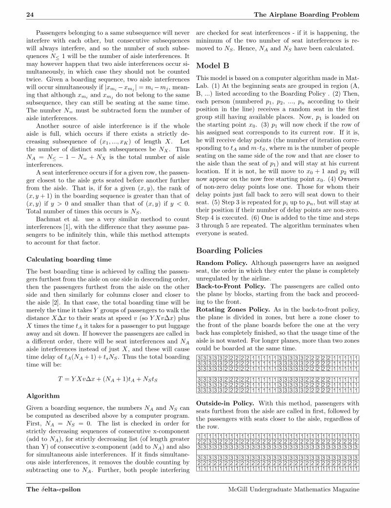
24 The Airplane Boarding Problem
Passengers belonging to a same subsequence will neverinterfere with each other, but consecutive subsequenceswill always interfere, and so the number of such subse-quences N≤ 1 will be the number of aisle interferences. Itmay however happen that two aisle interferences occur si-multaneously, in which case they should not be countedtwice. Given a boarding sequence, two aisle interferenceswill occur simultaneously if |xmi
−xmj| = mi −mj , mean-
ing that although xmiand xmj
do not belong to the samesubsequence, they can still be seating at the same time.The number N= must be subtracted form the number ofaisle interferences.
Another source of aisle interference is if the wholeaisle is full, which occurs if there exists a strictly de-creasing subsequence of (x1, ..., xK) of length X. Letthe number of distinct such subsequences be NX . ThusNA = N≤ − 1 − N= + NX is the total number of aisleinterferences.
A seat interference occurs if for a given row, the passen-ger closest to the aisle gets seated before another furtherfrom the aisle. That is, if for a given (x, y), the rank of(x, y + 1) in the boarding sequence is greater than that of(x, y) if y > 0 and smaller than that of (x, y) if y < 0.Total number of times this occurs is NS .
Bachmat et al. use a very similar method to countinterferences [1], with the difference that they assume pas-sengers to be infinitely thin, while this method attemptsto account for that factor.
Calculating boarding time
The best boarding time is achieved by calling the passen-gers furthest from the aisle on one side in descending order,then the passengers furthest from the aisle on the otherside and then similarly for columns closer and closer tothe aisle [2]. In that case, the total boarding time will bemerely the time it takes Y groups of passengers to walk thedistance X∆x to their seats at speed v (so Y Xv∆x) plusX times the time tA it takes for a passenger to put luggageaway and sit down. If however the passengers are called ina different order, there will be seat interferences and NA
aisle interferences instead of just X, and these will causetime delay of tA(NA + 1) + tsNS . Thus the total boardingtime will be:
T = Y Xv∆x + (NA + 1)tA + NStS
Algorithm
Given a boarding sequence, the numbers NA and NS canbe computed as described above by a computer program.First, NA = NS = 0. The list is checked in order forstrictly decreasing sequences of consecutive x-component(add to NA), for strictly decreasing list (of length greaterthan Y) of consecutive x-component (add to NA) and alsofor simultaneous aisle interferences. If it finds simultane-ous aisle interferences, it removes the double counting bysubtracting one to NA. Further, both people interfering
are checked for seat interferences - if it is happening, theminimum of the two number of seat interferences is re-moved to NS . Hence, NA and NS have been calculated.
Model B
This model is based on a computer algorithm made in Mat-Lab. (1) At the beginning seats are grouped in region (A,B, ...) listed according to the Boarding Policy . (2) Then,each person (numbered p1, p2, ..., pn according to theirposition in the line) receives a random seat in the firstgroup still having available places. Now, p1 is loaded onthe starting point x0. (3) p1 will now check if the row ofhis assigned seat corresponds to its current row. If it is,he will receive delay points (the number of iteration corre-sponding to tA and m ·tS , where m is the number of peopleseating on the same side of the row and that are closer tothe aisle than the seat of p1) and will stay at his currentlocation. If it is not, he will move to x0 + 1 and p2 willnow appear on the now free starting point x0. (4) Ownersof non-zero delay points lose one. Those for whom theirdelay points just fall back to zero will seat down to theirseat. (5) Step 3 is repeated for pi up to pn, but will stay attheir position if their number of delay points are non-zero.Step 4 is executed. (6) One is added to the time and steps3 through 5 are repeated. The algorithm terminates wheneveryone is seated.
Boarding Policies
Random Policy. Although passengers have an assignedseat, the order in which they enter the plane is completelyunregulated by the airline.Back-to-Front Policy. The passengers are called ontothe plane by blocks, starting from the back and proceed-ing to the front.Rotating Zones Policy. As in the back-to-front policy,the plane is divided in zones, but here a zone closer tothe front of the plane boards before the one at the veryback has completely finished, so that the usage time of theaisle is not wasted. For longer planes, more than two zonescould be boarded at the same time.
Outside-in Policy. With this method, passengers withseats furthest from the aisle are called in first, followed bythe passengers with seats closer to the aisle, regardless ofthe row.
The δelta-ǫpsilon McGill Undergraduate Mathematics Magazine
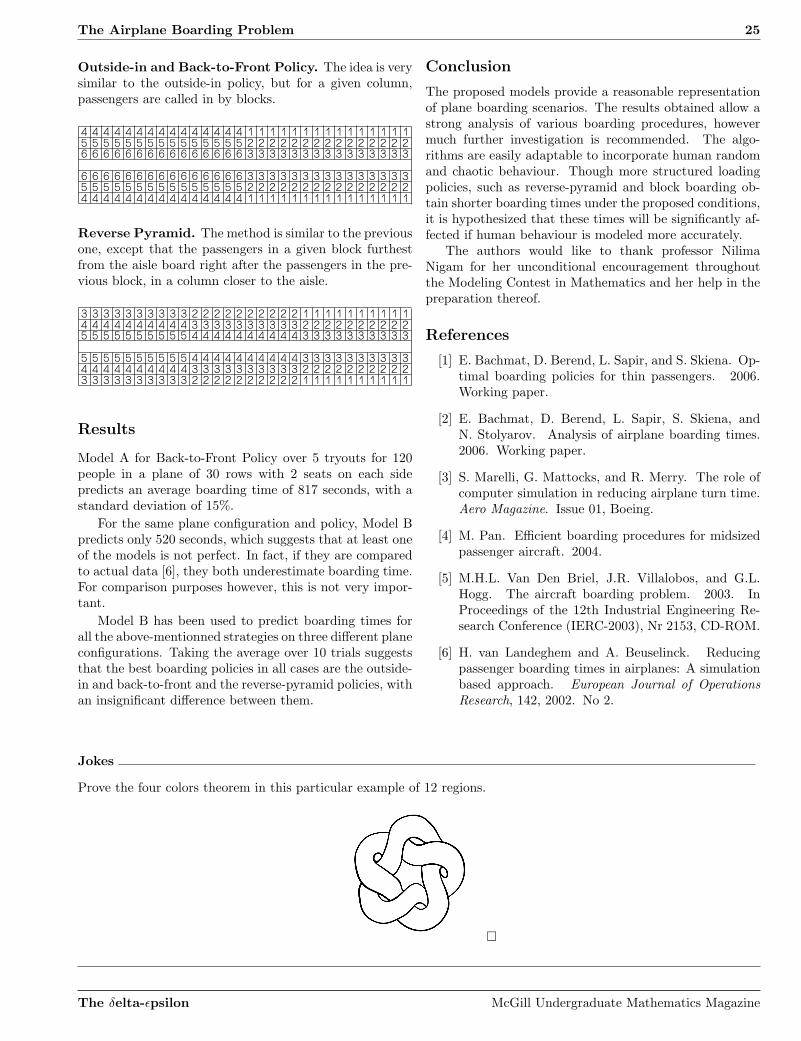
The Airplane Boarding Problem 25
Outside-in and Back-to-Front Policy. The idea is verysimilar to the outside-in policy, but for a given column,passengers are called in by blocks.
Reverse Pyramid. The method is similar to the previousone, except that the passengers in a given block furthestfrom the aisle board right after the passengers in the pre-vious block, in a column closer to the aisle.
Results
Model A for Back-to-Front Policy over 5 tryouts for 120people in a plane of 30 rows with 2 seats on each sidepredicts an average boarding time of 817 seconds, with astandard deviation of 15%.
For the same plane configuration and policy, Model Bpredicts only 520 seconds, which suggests that at least oneof the models is not perfect. In fact, if they are comparedto actual data [6], they both underestimate boarding time.For comparison purposes however, this is not very impor-tant.
Model B has been used to predict boarding times forall the above-mentionned strategies on three different planeconfigurations. Taking the average over 10 trials suggeststhat the best boarding policies in all cases are the outside-in and back-to-front and the reverse-pyramid policies, withan insignificant difference between them.
Conclusion
The proposed models provide a reasonable representationof plane boarding scenarios. The results obtained allow astrong analysis of various boarding procedures, howevermuch further investigation is recommended. The algo-rithms are easily adaptable to incorporate human randomand chaotic behaviour. Though more structured loadingpolicies, such as reverse-pyramid and block boarding ob-tain shorter boarding times under the proposed conditions,it is hypothesized that these times will be significantly af-fected if human behaviour is modeled more accurately.
The authors would like to thank professor NilimaNigam for her unconditional encouragement throughoutthe Modeling Contest in Mathematics and her help in thepreparation thereof.
References
[1] E. Bachmat, D. Berend, L. Sapir, and S. Skiena. Op-timal boarding policies for thin passengers. 2006.Working paper.
[2] E. Bachmat, D. Berend, L. Sapir, S. Skiena, andN. Stolyarov. Analysis of airplane boarding times.2006. Working paper.
[3] S. Marelli, G. Mattocks, and R. Merry. The role ofcomputer simulation in reducing airplane turn time.Aero Magazine. Issue 01, Boeing.
[4] M. Pan. Efficient boarding procedures for midsizedpassenger aircraft. 2004.
[5] M.H.L. Van Den Briel, J.R. Villalobos, and G.L.Hogg. The aircraft boarding problem. 2003. InProceedings of the 12th Industrial Engineering Re-search Conference (IERC-2003), Nr 2153, CD-ROM.
[6] H. van Landeghem and A. Beuselinck. Reducingpassenger boarding times in airplanes: A simulationbased approach. European Journal of OperationsResearch, 142, 2002. No 2.
Jokes
Prove the four colors theorem in this particular example of 12 regions.
¤
The δelta-ǫpsilon McGill Undergraduate Mathematics Magazine

26 Spectrum and Expansion of Biregular Graphs
Spectrum and Expansion of Biregular Graphs
Rosalie Belanger-Rioux and Ioan Filip
Graphs with a strong expansion property are extremely useful in many areas of mathematics andcomputer science, particularly in the design of efficient algorithms. It is, however, very difficultto explicitly construct infinite families of good expanders. In this paper, we study the spectrumof biregular graphs and show how it is related to their expansion coefficient. We also describe aconstruction of biregular expanders from elliptic curves. Finally, we present some experimentalresults on the second largest eigenvalues of biregular graphs with degrees 2 and 7.
Definition and preliminaries
A graph G = (V,E) consists of a set V of vertices and aset E ⊆ V × V of edges between the elements in V . Wesay that a graph G is bipartite and we write G = (L,R,E)if V can be partitioned into two subsets L and R (called“left” and “right” vertices) such that the edges in E arefrom elements of L to elements of R. Finally, we call abipartite graph a biregular graph if every left vertex hasdegree dL and every right vertex has degree dR (by degreeof v ∈ V we mean the number of edges in E incident tov). This implies that dL |L| = dR |R|.
An important property of graphs is the notion of expan-sion: how much larger than S ⊂ V can its set of neighborsbe. Graphs with a high expansion coefficient are extremelyuseful in computer science for the design of efficient algo-rithms, for combinatorial optimization and for construct-ing error-correcting codes, but they are also important inother fields like statistical physics.
Using a probabilistic approach, it is not difficult toprove the existence of infinitely many graphs with goodexpanding properties. However, explicit constructions offamilies of good expanders are hard to find and only ap-peared in the late 80’s (see [6]).
Our main interest is constructing biregular graphs withhigh expansion. The motivation for this particular classof graphs comes from applications where the structuresinvolved consist of two types of fundamentally differentnodes. For instance, when analyzing complex networkssuch as the Internet, one can distinguish between users andservers, viewed as vertices on a large graph. In this paper,we make rigorous the notion of expansion for a biregulargraph G and present some theoretical as well as experi-mental results relating expansion to the spectrum of G.
Definition 1. An (L,R, dL, dR, c) − expander is a bipar-tite graph on the sets of left vertices L and right verticesR, where the maximal degree of a left vertex is dL and themaximal degree of a right vertex is dR, such that dL ≤ dR
and for every X ⊂ L,
|∂(X)| ≥(
dL
dR+ c
(
1 − |X||L|
))
|X| . (1)
Here, ∂(X) = r ∈ R | ∃l ∈ X with (l, r) ∈ E, denotesthe set of neighbors of X.
Let G = (L,R,E) be a connected bipartite graphwith the sets L =
l1, . . . , l|L|
of left vertices and R =
r1, . . . , r|R|
of right vertices. (By connected we meanthat for all x, y in G, there exists a path in G from x toy.) We define the incidence matrix MG of G as follows
mGi,j =
1 (li, rj) ∈ E0 otherwise
.
Next, we define the adjacency matrix AG (note it is realand symmetric, so diagonalisable) such that
aGi,j =
1 (vi, vj) ∈ E0 otherwise
.
where vk = lk for 1 ≤ k ≤ |L| and vk′+|L| = rk′ for1 ≤ k′ ≤ |R|. In fact,
AG =
[
0 MM t 0
]
.
The eigenvalues of AG are called the spectrum of G. It iseasy to prove that the spectrum of G, a connected biregu-lar graph, is
√
dLdR = λ1 > λ2 ≥ . . . ≥ λn = −√
dLdR,
with λ 6= 0 being an eigenvalue if and only if −λ is aneigenvalue, if and only if λ is an eigenvalue of both M andMT . Note also that
A2G =
[
MMT 00 MT M
]
, (2)
so the ijth entry of A2G is the total number of paths of
length 2 between vi and vj , with any row or column sumequal to dLdR. It then follows that ±λ is an eigenvalueof AG if and only if λ2 is an eigenvalue of A2
G. Moreover,λ 6= 0 is an eigenvalue of A2
G if and only if it is an eigen-value of both MMT and MT M . Finally, we know that theeigenvector associated both with the largest eigenvalue of
AG and A2G is e1 = (1,...,1)√
|L|+|R|. The other vectors of the or-
thonormal eigenbasis of A2G will be called e2, . . . , e|L|+|R| .
We are now ready to prove the following theorem:
Theorem 1. Let G = (L,R,E) be a connected biregulargraph as defined above. Let λ2 = λ2(AG). Then G is an
(L,R, dL, dR, c)-expander, with c =dLdR−λ2
2
d2R
.
The δelta-ǫpsilon McGill Undergraduate Mathematics Magazine

Spectrum and Expansion of Biregular Graphs 27
Proof. (See [2]) Let A = A(G), and let X be a subset ofthe left vertices of G such that |X| ≤ α|L|, with x itscharacteristic vector (so the ith coordinate of x’s is 1 if
vi ∈ X, else it is 0). We have that xxT = ‖x‖2= |X|.
We shall bound |∂(X)||X| from below. Let C = xA. We know
that f(x) = x2 is a convex function, and so for any realnumbers ai, i = 1, . . . , k we have
(
k∑
i=1
a2i
)
≥ 1
k
(
k∑
i=1
ai
)2
.
Further, since there are precisely |∂(X)| coordinates Cj ofC that are not zero, we have:
‖C‖2=
|L|+|R|∑
j=1
C2j ≥
(
∑|L|+|R|j=1 Cj
)2
|∂(X)| =(|X| dL)
2
|∂(X)| ,
and so
|∂(X)||X| ≥ |X| d2
L
‖C‖2 . (3)
Remains to be found the required upper bound for ‖C‖2.
First, we expand x in terms of our orthonormal eigenbasisso that
AAT xT =
|L|+|R|∑
i=1
λ2i γiei.
Then,
‖C‖2= ‖xA‖2
= 〈xA, xA〉 = xAAT xT =
|L|+|R|∑
i=1
λ2i γ
2i .
Now, we know that,
γ1 = 〈x, e1〉 = xeT1 = |X|/
√
|L| + |R|,
so, since λ2 ≥ . . . ≥ λn,
‖C‖2 ≤ λ21γ
21 + λ2
2
|L|+|R|∑
i=2
γ2i
= γ21
(
λ21 − λ2
2
)
+ λ22 ‖x‖2
=|X|2
|L| + |R|(
dLdR − λ22
)
+ λ22 |X| .
Thus from 3 we obtain the following:
|∂(X)||X| ≥ d2
L|X|
|L|+|R| (dLdR − λ22) + λ2
2
or
∂(X) ≥ |X| d2L
α (dLdR − λ22) + λ2
2
for all X ⊆ L, |X| ≤ α|L|. Thus we have found a lowerbound for the expansion of subsets of the left vertices of
any connected biregular graph. Putting α = 1 and rear-ranging (see [1] for the case |L| = |R|) to obtain the formrequired by Definition 1, we get:
|∂(X)| ≥(
dL
dR+
(
dLdR − λ22
d2R
)(
1 − |X||L|
))
· |X| .
¤
Ramanujan graphs : definition and exam-
ples
We remind the reader that we are in fact interested inexplicit constructions of biregular graphs that are goodexpanders for any left size. Since a smaller second eigen-value implies a larger expansion, we would like to studythe asymptotic behavior of the second largest eigenvalueof a bipartite graph’s adjacency matrix as the left size ofthe graph grows. The following theorem is a generalisationof the Alon-Boppana bound for the eigenvalues of regulargraphs.
Theorem. Among the biregular graphs G = (L,R,E) wehave
lim inf|L|→∞
λ2(G) ≥√
dL − 1 +√
dR − 1.
This motivates in part the definition of Ramanujanbiregular graphs, graphs with their second largest eigen-value as small as possible in the asymptotic sense.
Definition 2. A biregular graph G = (L,R,E) is Ra-manujan if any non-trivial eigenvalue λ of AG satisfies
|√
dL − 1 −√
dR − 1| ≤ |λ| ≤√
dL − 1 +√
dR − 1.
We continue with two interesting examples of biregu-lar graphs. The first example is a specific infinite class ofbiregular graphs of left degree 2 and the second is basedon a construction using projective curves.
Example 1: Ramanujan graphs of left degree 2
Let n, k ∈ N with n ≥ k ≥ 1. Construct the graphG = (L,R,E;n, k) as follows.
Let L = 1, 2, . . . , n and R be the set whose elementsare the subsets of L of size k. Thus |L| = n and |R| =
(
nk
)
.An element x ∈ L is connected to an element S ∈ R ifand only if x ∈ S. The graph we obtain is biregular withdL =
(
n−1k−1
)
and dR = k.
Let M be the incidence matrix of G. Given i, j ∈ L ,there are precisely
#S ∈ R : i ∈ S, j ∈ S =
(
n − 2
k − 2
)
subsets of L of size k containing both i and j, so for i 6= j,this is also the number of walks of length 2 from i to j.
The δelta-ǫpsilon McGill Undergraduate Mathematics Magazine
28 Spectrum and Expansion of Biregular Graphs
Therefore, we have that
MM t =
(
n−1k−1
) (
n−2k−2
)
. . .(
n−2k−2
)
(
n−2k−2
) (
n−1k−1
)
. . .(
n−2k−2
)
......
. . ....
(
n−2k−2
) (
n−2k−2
)
. . .(
n−1k−1
)
=
(
n − 2
k − 1
)
In +
(
n − 2
k − 2
)
1 . . . 1...
. . ....
1 . . . 1
.
It is easy to see that the second eigenvalue of MM t is(
n−2k−1
)
and that its spectrum is
Spec(MM t) =
k
(
n − 1
k − 1
)
,
(
n − 2
k − 1
)
.
Consequently, by definition 2, our graph G =(L,R,E;n, k) is Ramanujan if and only if
√
(
n − 1
k − 1
)
− 1 −√
k − 1 ≤√
(
n − 2
k − 1
)
≤√
(
n − 1
k − 1
)
− 1 +√
k − 1.
Observe that for k = 2, these inequalities are trivial andthus the graphs G = (L,R,E;n, 2) are Ramanujan. More-over, note that the right inequality holds for any n, k withn ≥ k ≥ 1 and so by theorem 1, these graphs are relativelygood expanders.
Example 2: Biregular graphs from projectivecurves
Let F be the field with q elements and let P2(F) bethe projective plane over F. The general linear groupGLn+1(F) acts on A3\0 by multiplication by a matrixM ∈ GLn+1(F) and PGL3(F) = GL3(F)/F× acts similarlyon P2.
Let f(x, y, z) be a homogeneous polynomial of degreed = 3 and observe that the equation f(x : y : z) = 0 is welldefined. Denote by Zf (F) be the hypersurface of degree 3and dimension 1 given by
Zf (F) = x ∈ P2(F) | f(x) = 0.
We further assume that q > 16 and that f(x, y, z) is irre-ducible and non-singular on Zf (F), that is, on Zf ,
(
∂f
∂x,∂f
∂y,∂f
∂z
)
6= (0, 0, 0).
Now for every M ∈ PGL3(F), define Mf(x) =f(M−1x). Note that Mf is still a homogeneous polyno-mial of degree d and f(x) = 0 if and only if Mf(Mx) = 0.Therefore ZM f (F) = M · Zf (F). For simplicity, we write
S(M) for ZM f (F). Clearly, S(M) depends only on anM ∈ PGL3(F):
S(M) = M · S(I) = Mv | v ∈ S(I).
From our assumptions and by the theorems of Hasse-Weil and Bezout, we can conclude that S(M) = S(I)if and only if Mf = constant · f . We write g ∼ f forg = constant · f .
We can now construct the bipartite graph G =(L,R,E) as follows. The left vertices are in fact the setsS(M),
L = S(M) | M ∈ PGL3(F).Note that S(M) = S(N) if and only if N−1M ·S(I) = S(I),
if and only if N−1Mf ∼ f , and that PGL3 acts on L byM1 ·S(M2) = S(M1M2). The right vertices are the pointsin the projective plane, so R = P2(F). We put an edge(r, l) ∈ E where r ∈ R and l = S(M) ∈ L if r ∈ S(M),which is equivalent to the condition that M−1r ∈ S(I).
Clearly we have that |R| = q2 + q + 1. A computa-tion shows that the graph is biregular, with dL = #Zf (F).Also, we must have that
|L| =#PGL3(F)
#Stab(S(I)),
so in order to find dR we can compute the size of the stabi-lizer of S(I), namely #Stab(S(I)). Because f is not linear(as d > 1), we have
M ∈ PGL3(F) |M f ∼ f → Aut(Zf (F)),
where F is an algebraic closure of F. Applying once againBezout’s theorem we obtain
Mv = v,∀v ∈ Zf (F) ⇒ Mv = v,∀v ∈ Zf (F),
such that if v 7→ Mv is an automorphism of Zf (F), thenM must be a scalar matrix.
Let E[3](F) be the set of points of order 3 on E andassume the j-invariant for E, j(E), is neither 0 nor 1728.Observing that if M preserves E, then M must permutethe points of order 3 on E, we can conclude that
M ∈ PGL3 |M f ∼ f → 〈Id, i〉 · E[3](F),
where i is the hyperelliptic involution and Id is the trivialautomorphism. It is well known that |E[3](F)| = 1, 3 or 9.So if 3 ∤ N = q + 1 + err, and taking err = 0, q ≡ 1 mod3, we have a simple characterization of M ∈ PGL3(F) :Mf ∼ f because E[3](F) is trivial.
Now for r1 6= r2 ∈ R and given r3 6= r4, there exists amatrix M with Mr1 = r3 and Mr2 = r4. Consequently,we have that the number of common neighbors of r1 andr2, which is
u = |S(M) | M−1r1 ∈ S(I) ∩ S(M) | M−1r2 ∈ S(I)|,
is independent of r1, r2.
The δelta-ǫpsilon McGill Undergraduate Mathematics Magazine

Spectrum and Expansion of Biregular Graphs 29
Consider the matrix D = MM t with entries (d)rirj=
the number of walks of length 2 in the graph G = (L,R,E)between vertices ri and rj . Observe that
D =
dR u . . . u
u dR
......
. . . uu . . . u dR
= (dR − u)I + u
1 . . . 1...
. . ....
1 . . . 1
,
has spectrum
Spec(D) = dR−u+u
|R|, with multiplicity 1;0, with multip. |R| − 1.
(4)
Hence, the second largest eigenvalue of AG is λ2(AG) =√dR − u and according to the definition of biregular Ra-
manujan graphs (see definition 2), G = (L,R,E) is Ra-manujan if and only if
√
dR − 1 −√
dL − 1 ≤√
dR − u
≤√
dR − 1 +√
dL − 1,
which is equivalent to
dR + dL − 2−2√
(dR − 1)(dL − 1)
≤ dR(|R| − dL)
|R| − 1
≤ dR + dL − 2 + 2√
(dR − 1)(dL − 1).
The second inequality always holds; the first does notfor large values of q because
|L| =|PGL3(F)|Stab(S(I))
=q2(q3 − 1)(q3 − q)
Stab(S(I))= Θ(q8),
and so
dR =|L|dL
|R| = Ω(q6).
It can be verified in fact that asymptotically (as q →∞), the reverse inequality holds. Hence the graphs G =(L,R,E) described above are not Ramanujan as |F| → ∞.Expansion, however, is not reduced with the graphs notbeing Ramanujan (cf. theorem 1).
Experimental results
To conclude our article, let us present the computationalresults from our experiments on the distribution of theeigenvalues of biregular graphs. We constructed randomsimple connected biregular graphs, using the following idea(see [4]). First, build an array A of size dL|L|, with its firstdR cells containing r1, the next dR cells containing r2, etc.Then, permute the cells of A by a random permutationin SdL|L| to get the array A′, which defines a bipartite(multi)graph G, where the neighbors of l1 are the first dL
entries of A′, and so on. If G is a multigraph, return toarray A, take another permutation and check if it definesa simple connected bipartite graph.
We found that, among 159 random simple connectedbiregular graphs of degrees 2 and 7, with L = 1001, about79 of those were Ramanujan, while among 518 graphs ofleft size 39998, about 71 were Ramanujan. In fact, as isexpected, this percentage tends to slowly decrease as Lgrows larger (see Fig. 1).
Figure 1: The distribution of the second largest eigenvaluein random biregular graphs of left degree 2, right degree7 with left size 39998 (curve (a)) and left size 1001 (curve(b)). The vertical dotted line (c) indicates the Ramanujanbound.
Acknowledgments
We thank Professor Eyal Goren for his guidance and sup-port, which were crucial to our progress on this project.We are grateful to him for introducing us to this topic.We also thank Professor Nilima Nigam for her help withMatlab.
References
[1] Alon, Noga. “Eigenvalues and Expanders”, Combi-natorica , Vol. 6, 1986, p. 83-96.
[2] Tanner, R. Michael. “Explicit concentrators fromgeneralized N-gons”, SIAM J. Alg. Disc. Meth., Vol.5, No. 3, September 1984, p. 287-293.
[3] Hoory, S. Linial, N. Wigderson, A.“Expander graphsand their applications.” Bulletin of the AmericanMathematical Society, Vol. 43, No. 4, 2006, pp. 438-562.
[4] Jakobson, D. Miller, S. D. Rivin, I. Rudnick, Z.“Eigenvalue Spacings For Regular Graphs”, Emerg-ing Applications of Number Theory, Minneapolis,Vol. 109, 1996.
[5] Sole, P. “Ramanujan Hypergraphs and RamanujanGeometries.” Institute for Mathematics and Its Ap-plications, Vol. 109, 1999, pp. 583-590.
[6] Lubotzky, A. Phillips, R. and Sarnak, P. “Ramanu-jan Graphs”, Combinatorica, Vol. 8, 1988, pp. 261-277.
The δelta-ǫpsilon McGill Undergraduate Mathematics Magazine

30 Partially Observable Markov Decision Processes
Partially Observable Markov Decision Processes
Yang Li
In the field of artificial intelligence, many people are interested in finding new algorithms thatenable an agent to act intelligently in a world. Planning how to act in a stochastic world is amajor problem in the field. An intelligent agent must usually rely on an imperfect model of theworld to plan its actions. To improve the model used, the agent can learn a better model throughexperience; this makes learning another important problem in the field. Markov Decision Processes(MDPs) and Partially Observable Markov Decision Processes (POMDPs) are widely studied math-ematical models for these problems, originating from operations research [SS73]. POMDPs aremore expressive than MDPs because they model both partial observability (which can result, forexample, from having imperfect sensors) and probabilistic transitions (which are the result of theenvironment being stochastic). Unfortunately POMDPs are much harder to learn and to use forplanning. In this paper we present a new algorithm for learning POMDPs from data. The mainidea is to work with histories of actions and observations. We show that the new representationcan be used successfully to plan a good behavior.
Background
MDPs are formally represented as a 4-tuple(A,S, P (·), R(·)), where A is the action space, S is the statespace, P is the transition function P : S × A × S → [0, 1]that gives the probability that an action a will take theagent from state s to state s′ and R is the reward functionR : S → R which gives the agent’s immediate reward aftermoving to state s [SB98]. On every time step t, the agentwill observe the state of its environment, st and pick anaction at. This will cause the environment to transitionto a new state st+1 (determined by P ) and the agent willreceive a reward rt+1 determined by R. The behavior ofan agent can be described by a policy π : S → A thatspecifies what action should be taken in each state. Thevalue function V π : S → R expresses how good it is tobe in a certain state s if policy π will be used to chooseactions. It is defined as the expected value of the sum ofrewards that will be obtained when starting in s. In anMDP with a finite state and action set there is a uniqueoptimal value function, V ∗, and a corresponding optimalpolicy π∗.
For MDPs with continuous or large discrete state space,it is often handy to use state aggregation as it can re-duce the state space to a constant number of aggregatesG [SB98]. An aggregate G is a set of states combinedtogether to have a single value, and thus optimal action.Clearly, given an optimal policy π∗ over a non-aggregatedstate space and an optimal policy π′∗ over an aggregatedstate space, the expected value V π∗
(s) ≥ V π′∗
(s) ∀s ∈ S.This is because, if an aggregate contains states with a dif-ferent optimal action under π∗, at least one of these stateswill be forced to take a non-optimal action under π′∗.
This introduces the idea of splitting the state aggre-gates into smaller state aggregates. Since splitting willnever decrease the performance of the optimal policy, bysplitting aggregates we can improve the optimal policy.However, we do not want to split aggregates in which the
optimal policy is the same after splitting. In other words,we hope to split aggregates in such a way that the expectedreturn is significantly improved.
A POMDP is simply an MDP, but instead of beingable to observe the states, the agent is only able to ob-serve some features related to the state, according to someprobability distribution. Since the agent may observe cer-tain features of a state, but not enough to distinguish allstates from one another [KLC98], one set of features maymatch several different states. This induces state aliasingover observation features. Thus, we would like to repre-sent each state as an unique history of observations andactions, or at least, separate the aliased states to maxi-mize the value function.
For this to be possible, we assume a weaker version ofthe Markovian property. Instead of assuming the Marko-vian property that states that future observations and ex-pected reward depend only on the present observation andnot on any past observations [SB98], we assume that thefuture observations and expected reward depend only onthe past n observations (and actions) and not on any an-terior ones.
Under this assumption, which is much more reasonablethan the original one, we built an algorithm that enhancesa history by one unit of experience each time it thinks itis useful for maximizing the expected return.
Problem and Approach
For many problems, we would like our agents to be ableto improve their policy and internal world representationin an online fashion, as they observe new data. We expectthe agent to be able to observe features in the past thatcan help it guess in which state it is at the present time,and thus determine which action it should undertake next.
The δelta-ǫpsilon McGill Undergraduate Mathematics Magazine

Partially Observable Markov Decision Processes 31
Updating the Variable Length Histories Table(VLHT)
A history is a sequence of action-observation pairs. Ouralgorithm will maintain a table of histories, such that eachentry corresponds to a distinct state as perceived by theagent. The agent will decide what histories should be in-cluded in the table based on the data it observes. Eachentry in the VLHT will have an associated value (which isthe estimate of expected return if the agent acts accordingto policy π from that point on, having that history) anda corresponding action. In our approach, the agent willgather data in episodes, where each episode consists of atmost m steps. After m steps or after reaching a goal state,the episode ends and the return information for all the his-tories in the VLHT which have been experienced duringthe episode are updated.
Enhancing histories
Enhancing histories is done by adding more action-observation pairs (thus making it longer). Deciding whichhistory to enhance is the trickiest part of the problem. Weset a threshold on the variance of the returns followinga history to determine whether the history is representa-tive of a single state (or a group of states which have thesame optimal action), or if it may correspond to differentstates. This technique is simple, but it is very efficient andworks well enough for our purpose. To do this, the agentremembers the different observations after each of its his-tories and keeps the sum and squared sum of the returnsthat have been obtained so far for each history, in order tocompute the variance quickly and whenever necessary.
Our agent is expected to be able to learn the lengthof the history necessary to distinguish aliased states whichimpair the performance of the agent. The length of thehistory will vary depending on the world and the featuresobservable by the agent. The agent should stop adding ex-perience units to any history after the optimal policy canbe represented.
Algorithm 1 Variable Length History Algorithm
VLHT ← new table, while conditions C not met do
Learn(randomAction, m, parameters)end while
The VLH-algorithm
As seen in Algorithm 1 and 2, the VLH-algorithm is recur-sive and tells the agent to stop when the number of stepsremaining decreases to 0 or when the goal is reached.
In the recursion step of the algorithm, the agent, whenat state s, uses its sensors to gather observation o and un-dertakes an action a After ending in state s′, it will, again,use its sensors to observe o′ and decide which action to takenext. Actions are chosen in an ǫ-greedy fashion according
to the VLH table; that is, the best action as predicted bythe table is chosen with probability (1−ǫ) and a uniformlyrandom action is chosen with probability ǫ.
Each entry of the VLH table is defined recursively:(o, a) is a valid entry and e(o, a) is a valid entry if e is avalid entry. Thus, each entry of the table will be a sequenceof experience units, (o, a), of different lengths. Since thehistory of the actions of an agent is also a sequence of ex-perience units, by comparing the value of each sequencee(ot, a1), e(ot, a2), · · · , e(ot, an), we know which action ai
to choose when we observe ot and have history e.
Algorithm 2 Recursive Function of the VLH-algorithm
Learn(action, m, parameters)
o, a, s, r ← observation, action, state, rewards′ ← state after undertaking action a in sa′ ← action selected in a randomized way.o′, r′ ← observation at state s′, reward gainedh ← longest history in VLHT matching agent’sif agent in goal state then
s ← random statereturn reward
else if m = 0 thenreturn reward
end ifMCreturn ← r + γLearn(a′, m − 1, parameters)if (o, a) in VLHT then
error ← r + γMCreturn − VLHT[h]Update VLHT[h] (
∑
MCret,∑
MCret2)for all sub-histories(*) sh of h do
VLHT[sh] ← VLHT[sh] +α errorend for
elseVLHT[(o, a)] ← MCreturn
end ifif h has unusual outcomes then
h′ ← h+unit < o, a > followed by hVLHT[h′], ET[h′] ← MCreturn, 0
end if
(*) sub-histories of h which ends with the same (o, a) tupleas h.
An important property to notice is that the shorterlength histories will never be made obsolete by longer ones,and are quite useful, due to the fact that the agent does notalways have a history which matches an entry of the table.Furthermore, whenever the agent starts fresh, or thinksthat its history is inaccurate due to noise, the agent maypurposefully delete its history and start collecting experi-ence units from scratch; this will require knowledge aboutthe short histories.
When an episode is over, the agent will update its ta-ble and representation of the world. Updating the tableis straightforward as we update the history and all sub-histories equally by r+γMCreturn − VLHT[h], a commonerror term. We also update the sum of the returns and the
The δelta-ǫpsilon McGill Undergraduate Mathematics Magazine

32 Partially Observable Markov Decision Processes
sum of squared returns for each observation following forthe corresponding VLHT table entry.
The last and key part of the algorithm remains. In or-der to determine which history to enhance, we use the sumand sum squared of the Monte Carlo returns and calculatea variance. Clearly, aliased states with different optimalpolicy or very different optimal returns, will have variancethat is very high, and conversely, non-aliased states shouldhave very similar returns, thus low variance.
Results and Analysis
To test the VLH-algorithm, we use a simple π shaped grid-world with 9 states (Figure 1). The agent is equipped witha compass and can detect in which direction it can move,thus North, South, East, West form the whole actionspace A and o ⊂ A is an observation.
Figure 1: Grid-world (π shaped) with 3 pairs of aliasedstates (2 & 4, 6 & 7, 8 & 9)
Figure 2 shows the performance of the true, state-basedoptimal policy (horizontal top line) compared to the per-formance of policies found by our algorithm (averaged over30 independent runs). As we can see, the average per-formance of the near-optimal policy was not significantlybetter than the one of the policies found by the VLH-algorithm. This is really encouraging, given that VLH con-structs all its representation from observed data, withouthaving any prior knowledge about the environment.
Discussion
The first version of the VLH-algorithm seems promisingas it is simple and yet able to learn in environments withuncertainty. McCallum proposed a similar algorithm inhis PhD thesis; however, the VLH- algorithm has a dif-ferent approach for estimating which histories should beenhanced.
There are many adjustments which can improve theperformance of the algorithm. The most important one is
merging similar histories together. This would lower boththe space complexity and the time complexity of the algo-rithm.
Figure 2: Performance graph
The project was realized during Summer 2007 andfunded by a NSERC USRA supervised by Dr. Doina Pre-cup.
References
[SS73] R. D. Smallwood and E. J. Sondik. The optimalcontrol of partially observable Markov processes over afinite horizon. Operation research, 1973.
[M05] K. P. Murphy. A Survey of POMDP SolutionTechniques. 2005.
[SB98] R. Sutton and A. Barto. Reinforcment Learn-ing: An Introduction. MIT Press, 1998.[McC95] A. McCallum. Reinforcement Learning with Se-lective Perception and Hidden State. PhD thesis, Univ.Rochester, 1995.
[KLC98] L. P. Kaelbling, M. Littman, and A. Cassandra.Planning and acting in partially observable stochastic do-mains. Artificial Intelligence, 101, 1998.
Jokes
Relations between pure and applied mathematicians are based on trust and understanding. Namely, pure mathe-maticians do not trust applied mathematicians, and applied mathematicians do not understand pure mathematicians.¤
The δelta-ǫpsilon McGill Undergraduate Mathematics Magazine

Fun Results in Algebraic Topology 33
Fun Results in Algebraic Topology
Agnes F. Beaudry
Algebraic topology provides very elegant tools to prove fun results such as Brouwer’s Fixed PointTheorem, which says that every continuous function from the disk to itself has a fixed point; or theBorsuk-Ulam theorem, which states that every continuous map from the sphere to R2 sends a pairof antipodal points to the same point in R2. I want to give here a taste of the machinery. To dothis, I will provide an intuitive proof of Brouwer’s Fixed Point theorem, which illustrates the basicideas which are at the root of algebraic topology.
Introduction
Throughout, S1 denotes a circle, D2 a closed disk andI = [0, 1] the closed unit interval. You can picture S1
in R2 as the curve x2 + y2 = 1 and D2 as the set(x, y)|x2 + y2 ≤ 1.
My goal is to give an intuitive idea of how one provesthe following theorem using algebraic topology. You mighthave seen it proved using more analytic tools in one of theundergraduate analysis classes. The point here is not somuch the result (although it’s a great result), but the toolsused to prove it.
Theorem. Brouwer’s Fixed Point Theorem Everycontinuous map ϕ : D2 → D2 has a fixed point, i.e., thereis an x ∈ D2 such that ϕ(x) = x.
I will prove Brouwer’s fixed point theorem by contra-diction, showing that, if there is a map ϕ : D2 → D2 whichhas no fix point, then we can continuously deform the diskD2 onto the circle S1. Some key topological properties ofS1 make this impossible: this is what we will be lookingat. The proofs will not be rigorous, although everythingwe say can be made rigorous with more machinery.
Paths
We start with X, a topological space. Formally, a pathfrom x to y on X is a continuous map g : I → X suchthat g(0) = x and g(1) = y. You can picture this as aparametrized curve joining two points. An example is astraight line in R2 joining x and y, which we can write asl : I → R2
l(t) = ty + (1 − t)x.
At t = 0, the line is at x, and at t = 1, it is at y.
Another example is the arc of a circle. Say x = (1, 0)and y = (−1, 0). Then we can join x and y by an arc ofthe unit circle. We can parameterize this as g : I → R2
g(t) = (cos(πt), sin(πt)).
Similarly we can join x and y by h : I → R2
h(t) = (cos(−πt), sin(−πt)).
Figure 1: Some paths in R2.
With the line l(t) = ty + (1 − t)x, we now have threepaths joining the points (±1, 0). In fact, there are uncount-ably many such paths. How different are they? Supposewe take a rope and pin one end to (1, 0) and pin the otherend to (−1, 0). We would like to say that it does not mat-ter where we set down the rope on the plane, how muchwe stretch it, or how we move it around (without liftingit): as long as we do not cut it, it remains the same ropejoining the same two points.
We do the same thing for paths and say that two pathsare equivalent, or homotopic, if we can continuously de-form one path into the other, without cutting our curves.More precisely, two paths are homotopic if there is a familyof intermediate curves continuously transforming one pathinto the other.
For a general topological space X we say the following:let g0 : I → X and g1 : I → X be continuous maps joiningx and y, i.e., gi(0) = x and gi(1) = y for i = 1, 2. Wesay that g0 and g1 are homotopic if there exists a fam-ily of continuous maps F (s, t) = fs(t) : I × I → X suchthat F (0, t) = f0(t) = g0(t), F (1, t) = f1(t) = g1(t) withF (s, 0) = x and F (s, 1) = y for all s ∈ I. This means thatthe first curve is g0, the last curve g1, and each intermedi-ate curve is a path joining x and y.
For example, letting l(t) and g(t) be the paths in R2
described above, then
F (s, t) = fs(t) = (cos(πt), s · sin(πt))
The δelta-ǫpsilon McGill Undergraduate Mathematics Magazine

34 Fun Results in Algebraic Topology
is a homotopy from l(t) to g(t).
Figure 2: A homotopy between g0 and g1.
The idea is this: pick any two points on your surface X,say a torus, draw two curves or paths lying on your surfacejoining the points. If you can stretch and twist and shrinkthe first curve into the other, without cutting it, then thetwo paths are homotopic. The left-hand picture belowshows two paths on the torus which are homotopic, whilethe right-hand picture shows two non-homotopic paths.
Figure 3: Homotopic and non-homotopic loops on thetorus.
Loops
Now fix a point x0 on your surface X. Paths which startand end at x0 are called loops with base point x0.
Definition 1. A loop is a path f : I → X such thatf(0) = f(1).
We want to know which loops are homotopic. Let’s dothe exercise on D2. Let x0 be the center of this disk. Thefirst loop is the ‘do-nothing’ loop, i.e., c : I → D2 with
c(t) = x0, ∀t ∈ I.
Take another loop based at x0, say f : I → X. Can wedeform f into the constant loop, i.e., can we shrink f to thecenter? Intuitively, this seems possible. Indeed, since D2 isconvex we can join any point on the loop f to the point x0
by a straight line, and then shrink f to x0 along these lines.The homotopy is given by F (s, t) = fs(t) : I × I → D2
fs(t) = sx0 + (1 − s)f(t).
What this means is that any loop based at x0 on thedisk D2 is homotopic to the constant loop at x0. The onlything we used to prove this is that, for any point x ∈ D2,there is a line joining x and x0. This holds for any pointon the disk D2, not just the center. Hence the loops basedat any point are homotopic to the constant loop at thatpoint. We state this result as a lemma, for it will be usefullater:
Figure 4: Homotopy from f to the constant loop at x0.
Lemma 1. Any loop f : I → D2 based at x is homotopicto the constant loop at x.
Another example is R2. Pick any point x0 ∈ R2. Asfor the disk, any point can be joined to x0 by a straightline. Hence 1 gives a homotopy from any loop at x0 to theconstant loop at x0.
Though it seems intuitively obvious, it is harder toshow that any loop f : I → S2 based at x0 is homotopic tothe constant loop at x0. Here S2 denote a sphere, whichyou can visualize in R3 as the surface x2 + y2 + z2 = 1.
In all these examples, we could shrink the loops to apoint. This is not always the case. The loops on a torus T 1
are not all trivial. Let x0 ∈ T 1. Let f be the loop based atx0 which wraps around the torus in the vertical directionand h the loop which wraps around T 1 in the horizontaldirection (see the figure of the torus above).
The loop h is not homotopic to the constant loop, sincewe cannot pull it across the hole back to the point x0. It”contains” the hole while the constant loop does not. Thisis a fundamental difference between the two loops. On theother hand, the loop f does not surround the hole, but itencloses the inside of the torus. To shrink it to the con-stant loop, we would need to cut through the torus. Hencef and h are both essentially different from the constantloop at x0. Are they homotopic to each other? The an-swer is no, since h contains the hole of the torus and f doesnot. To deform h into f , we would need to pull it throughthe hole. Similarly, we cannot deform f into h. Therefore,we have at least two non-homotopic loops which are nothomotopic to the constant loop. Of course, we can makethese intuitive arguments rigorous.
The δelta-ǫpsilon McGill Undergraduate Mathematics Magazine
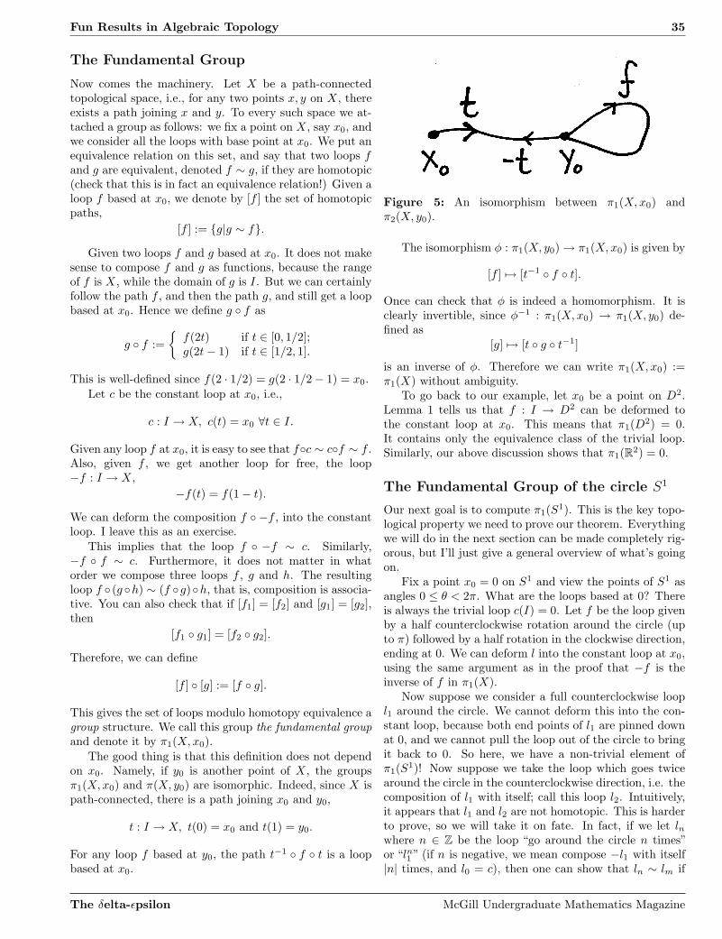
Fun Results in Algebraic Topology 35
The Fundamental Group
Now comes the machinery. Let X be a path-connectedtopological space, i.e., for any two points x, y on X, thereexists a path joining x and y. To every such space we at-tached a group as follows: we fix a point on X, say x0, andwe consider all the loops with base point at x0. We put anequivalence relation on this set, and say that two loops fand g are equivalent, denoted f ∼ g, if they are homotopic(check that this is in fact an equivalence relation!) Given aloop f based at x0, we denote by [f ] the set of homotopicpaths,
[f ] := g|g ∼ f.
Given two loops f and g based at x0. It does not makesense to compose f and g as functions, because the rangeof f is X, while the domain of g is I. But we can certainlyfollow the path f , and then the path g, and still get a loopbased at x0. Hence we define g f as
g f :=
f(2t) if t ∈ [0, 1/2];g(2t − 1) if t ∈ [1/2, 1].
This is well-defined since f(2 · 1/2) = g(2 · 1/2 − 1) = x0.
Let c be the constant loop at x0, i.e.,
c : I → X, c(t) = x0 ∀t ∈ I.
Given any loop f at x0, it is easy to see that fc ∼ cf ∼ f .Also, given f , we get another loop for free, the loop−f : I → X,
−f(t) = f(1 − t).
We can deform the composition f −f , into the constantloop. I leave this as an exercise.
This implies that the loop f −f ∼ c. Similarly,−f f ∼ c. Furthermore, it does not matter in whatorder we compose three loops f , g and h. The resultingloop f (g h) ∼ (f g)h, that is, composition is associa-tive. You can also check that if [f1] = [f2] and [g1] = [g2],then
[f1 g1] = [f2 g2].
Therefore, we can define
[f ] [g] := [f g].
This gives the set of loops modulo homotopy equivalence agroup structure. We call this group the fundamental groupand denote it by π1(X,x0).
The good thing is that this definition does not dependon x0. Namely, if y0 is another point of X, the groupsπ1(X,x0) and π(X, y0) are isomorphic. Indeed, since X ispath-connected, there is a path joining x0 and y0,
t : I → X, t(0) = x0 and t(1) = y0.
For any loop f based at y0, the path t−1 f t is a loopbased at x0.
Figure 5: An isomorphism between π1(X,x0) andπ2(X, y0).
The isomorphism φ : π1(X, y0) → π1(X,x0) is given by
[f ] 7→ [t−1 f t].
Once can check that φ is indeed a homomorphism. It isclearly invertible, since φ−1 : π1(X,x0) → π1(X, y0) de-fined as
[g] 7→ [t g t−1]
is an inverse of φ. Therefore we can write π1(X,x0) :=π1(X) without ambiguity.
To go back to our example, let x0 be a point on D2.Lemma 1 tells us that f : I → D2 can be deformed tothe constant loop at x0. This means that π1(D
2) = 0.It contains only the equivalence class of the trivial loop.Similarly, our above discussion shows that π1(R
2) = 0.
The Fundamental Group of the circle S1
Our next goal is to compute π1(S1). This is the key topo-
logical property we need to prove our theorem. Everythingwe will do in the next section can be made completely rig-orous, but I’ll just give a general overview of what’s goingon.
Fix a point x0 = 0 on S1 and view the points of S1 asangles 0 ≤ θ < 2π. What are the loops based at 0? Thereis always the trivial loop c(I) = 0. Let f be the loop givenby a half counterclockwise rotation around the circle (upto π) followed by a half rotation in the clockwise direction,ending at 0. We can deform l into the constant loop at x0,using the same argument as in the proof that −f is theinverse of f in π1(X).
Now suppose we consider a full counterclockwise loopl1 around the circle. We cannot deform this into the con-stant loop, because both end points of l1 are pinned downat 0, and we cannot pull the loop out of the circle to bringit back to 0. So here, we have a non-trivial element ofπ1(S
1)! Now suppose we take the loop which goes twicearound the circle in the counterclockwise direction, i.e. thecomposition of l1 with itself; call this loop l2. Intuitively,it appears that l1 and l2 are not homotopic. This is harderto prove, so we will take it on fate. In fact, if we let lnwhere n ∈ Z be the loop “go around the circle n times”or “ln1 ” (if n is negative, we mean compose −l1 with itself|n| times, and l0 = c), then one can show that ln ∼ lm if
The δelta-ǫpsilon McGill Undergraduate Mathematics Magazine

36 Fun Results in Algebraic Topology
and only if m = n. Also, these are the only equivalenceclasses, i.e., if f : I → S1 is a loop based at 0, then f ∼ lnfor some n ∈ Z.
Let me give a more precise idea of what’s going on.We look at the map f : R → S1 define by ϕ(x) = e2πix.This map sends all the integers to 1. Also, if we takea small enough neighborhood of a point x in R, sayIx = (x − 1/2, x + 1/2), the restriction of ϕ to Ix is ahomeomorphism onto its image. Hence ϕ is a local home-omorphism. We say that ϕ is a covering map of S1. Nowit’s a general fact that any loop γ on X can be lifted toa unique path in R starting at 0. That is, there exists aunique path g(t) in R such that g(0) = 0 and ϕ g = γ.
Letting γ0 be loop in S1, and let g0 be this unique path.Since γ0(1) = 1, it must be that g0(1) = n ∈ Z. If γ1 ishomotopic to γ0, the homotopy γs(t) lifts to a family gs(t)of continuous maps from g0 to g1 where g1 is the uniquelift of γ1 starting at 0. But since γs(1) = 1 for all s, wehave gs(1) ∈ Z for all s. We know that g0(1) = n ∈ Z,hence by continuity, it must be that g1(1) = n.
An isomorphism from π1(S1) to Z is given by associ-ating to each equivalence class of loops this integer. Westate this as a theorem:
Theorem. The fundamental group of the circle π1(S1) is
isomorphic to Z.
Retracts
Suppose we have a topological space X, and a subset A ofX (to which we give the subspace topology.) It might bepossible to retract X onto A, i.e., to shrink X to A, as inthe following picture.
Figure 6: A retract of X onto a subspace A.
To make this idea concrete, we define a retraction of atopological space X onto a subspace A to be a continuousfunction r : X → A, such that r restricts to the identitymap on A: r|A = idA.
Why do we care about retractions in the context of thefundamental group? Suppose A is a subspace of X, and gand h are paths in A. It might be ambiguous whether ornot they are homotopic by looking at A only. However, ifX retracts onto A, and as paths of X, g and h are homo-topic, we can conclude that g and h are homotopic in Aalso. This is what the following lemma says.
Lemma 2. Let X and A be as above, and let g : I → Aand h : I → A be paths in X with image in A. Supposeg and h are homotopic when viewed as paths in X, i.e.,there is a homotopy ft : I → X, from g to h. If there isa retraction r : X → A of X onto A, then the family ofmaps r ft : I → A is a homotopy of g and h in the spaceA.
The next proposition is the key to the proof of theo-rem , and this is here all the work pays off. The proof oftheorem is just the usual gymnastic of mathematics withthis proposition.
Proposition 1. There is no retraction of D2 onto S1.
Proof. For the sake of contradiction, suppose that such aretraction r existed. Consider the loops l1 and l0 based at0 on S1. We argued above that they represent distinct ho-motopy classes of π1(S
1). As paths on D2, lemma 1 showsthat there is a homotopy ft : I → D2 such that f0 = l1 andf1 = l0. Consider, r ft : I → S1, t ∈ I. By proposition2, this is a homotopy of l1 and l0 in S1! But l0 and l1 arenot homotopic in S1, a contradiction. Therefore, there isno such retraction r. ¤
Figure 7: A would-be retract of D2 onto S1.
As promised, here’s a proof of theorem
Proof. Brouwer’s Fixed point TheoremSuppose that ϕ : D2 → D2 is a continuous map which
has no fixed point. This means that x 6= ϕ(x) for allx ∈ D2, so we can draw a ray starting at ϕ(x) goingthrough x. This ray must meet the boundary of D2,namely S1, at one and only one point xr. Let r : D2 → S1
be defined by r(x) = xr (see figure below). This map isclearly continuous, because ϕ(x) is continuous. What doesit do to S1? If x ∈ S1, draw the ray starting from ϕ(x)passing through x. This ray meets S1 in one point xr.Clearly xr = x. Therefore r(x) = x. Hence r|S1 = idS1 .This means that r is a retraction of D2 onto S1, contra-dicting proposition 1. Therefore, all maps ϕ : D2 → D2
have a fix point. ¤
The δelta-ǫpsilon McGill Undergraduate Mathematics Magazine

Fun Results in Algebraic Topology 37
Other Interesting Results
Now that was just to give you a taste of what’s going on.The essential element was that π1(S
1) ≃ Z. As a con-clusion, I state here are a few other interesting theoremswhich are consequences of that fact.
Theorem. The Borsuk-Ulam Theorem For every con-tinuous map ψ : S2 → R2, there are antipodal points x and−x on S2 such that ψ(x) = ψ(−x).
Corollary 1. Whenever three closed sets A1, A2 and A3
have the property that S2 = A1∪A2∪A3, then at least oneof the sets Ai contains a pair of antipodal points, x and−x.
Theorem. Hamburger Theorem If A1, A2 and A3 areclosed and bounded sets in R3, there exists a plane which
cuts each Ai into two parts of equal measure.
Theorem. Fundamental Theorem of Algebra Everynon-constant polynomial f(x) ∈ C[x] has a root. That is,there is an α ∈ C such that f(α) = 0.
This article comes from notes written for a mini-lectureI gave at the Program for Young Scientists (PROMYS)at Boston University. I would like to thank prof. GlennStevens and everyone involved in PROMYS for hostingsuch a great program and making these mini-lectures pos-sible.
References
1. Allen Hatcher, Algebraic Topology, Cambridge Uni-versity Press, Cambridge, 2001
Jokes
An engineer, a physicist and a mathematician find themselves in an anecdote, indeed an anecdote quite similar tomany that you have no doubt already heard. After some observations and rough calculations the engineer realizes thesituation and starts laughing. A few minutes later the physicist understands too and chuckles to himself happily as henow has enough experimental evidence to publish a paper.This leaves the mathematician somewhat perplexed, as he had observed right away that he was the subject of ananecdote, and deduced quite rapidly the presence of humor from similar anecdotes, but considers this anecdote to betoo trivial a corollary to be significant, let alone funny. ¤
A mathematician organizes a lottery promising an infinite amount of money. Naturally, a lot of people buy tickets andthe mahematician earns a lot of money from the sales. When the lucky winner is finally announced, he goes to see themathematician, eager to get his prize. The mathematician looks at him calmly and says: “Here’s one dollar. Comeback tomorrow and I’ll give you half a dollar. Then the day after I’ll give you 1
3 of a dollar...” ¤
A lecturer tells the students to learn the phone-book by heart.The mathematicians are baffled: ‘By heart? Are you kidding?’The physics students ask: ‘Why?’The engineers sigh: ‘Do we have to?’The chemistry students ask: ‘Until next Monday?’The accounting-students (scribbling): ‘Until tomorrow?’The medicine students ask: ‘Should we start on the Yellow Pages?’The laws students answer: ‘We already have.’ ¤
The δelta-ǫpsilon McGill Undergraduate Mathematics Magazine


Mathematical Digest 39
Mathematical Digest
Nan Yang
Modern mathematics can be very abstract. A layman flipping through a mathematics textbookmay be so overwhelmed by the formalism that she loses sight of the very ideas which the formalismis trying to capture, even though the ideas themselves may be very intuitive and simple. In thisissue of Mathematical Digest we will take a look at two of them, isomorphisms and homomorphisms,from a non-mathematical perspective.
Isomorphism
The word ‘isomorphic’ appears in many courses describ-ing many different things. You may hear it in set theorydescribing ordered sets, or linear algebra describing vectorspaces, or abstract algebra describing groups, rings, fields,etc. You probably already know what it means: two thingsare isomorphic if they are, in the context of interest, thesame thing. Take, for example, chess (perhaps the bestexample available). Observe the following picture:
Figure 1: Chess
The picture on the left is a standard chessboard, madeof wood; the picture on the right is a chessboard madeout of, well, sidewalk. Yet we say that they are the ‘iso-morphic’, that they are the same game. Intuitively, this isbecause if you were to place them side by side, each moveon one corresponds uniquely to a move on the other. Agame to which chess is not isomorphic is, for instance, tic-tac-toe: for one thing, tic-tac-toe has no pieces to move!
It is possible to make the notion of isomorphism ofgames more rigorous as follows. The chessboard can be inone of finitely many states. At every stage the chessboardis in a given state. It is possible to move from one stateto another given that there is a single piece on the firststate that can be moved to a corresponding piece on thesecond state by a legal move. We then connect these twostates. If we represent the states by nodes, and the pos-sibility of ‘moving’ from one state to another by an edge,then we can think of Chess as a very large tree (of graphtheory), where repeated moves such as a knight movingback and forth between two positions is described by aninfinite branch. Then, given any game which has the aboveproperties (states, transition of states, etc), we can assign aunique tree to that game, up to isomorphism (this isomor-phism is well defined, for more information see a textbookon graph theory). Two games are isomorphic, then, whenthe trees assigned to them are isomorphic.
But I digress. What else can be a good, concrete anal-ogy for ‘isomorphism’? Let’s look at something a littlemore esoteric, and perhaps a bit far-fetched.
Beethoven’s 6th symphony is written in F major. Itsfirst few notes are:
Figure 2: Pastoral
But suppose it were written in some other key, say Cmajor. Of course, it certainly would sound different if itwere written in C major. And any music student would ar-gue with me that if it were performed in C major, it is notthe same piece of music. But I can dare say that those twopieces are ‘isomorphic’. How so? Because you can literally‘translate’ one into the other by ‘shifting’ notes up or down(the technical details will not be discussed here) and thusinformation is not lost in translation. If for some reasonthe only surviving copy of the score for the symphony hasbeen ‘shifted down’ so that it’s in C major, but we knowthat it should be in F major, we can easily translate itback to F major without loss of information. In this sense,the two pieces of music are ‘isomorphic’.
I mentioned the loss of information, because this is im-portant for the next concept that we will be discussing,homomorphism.
Homomorphism
You may have encountered homomorphisms before isomor-phisms because isomorphisms are, usually, ‘bijective homo-morphisms’. Therefore homomorphisms are more general.There is a very simple and concrete illustration of the ideathat two things are homomorphic: acronyms.
Figure 3: PHP
The δelta-ǫpsilon McGill Undergraduate Mathematics Magazine

40 Mathematical Digest
See? Think of the set of finite sequences of letters with-out spaces (i.e., ASDF, WADS, AGEFAWE) as having a‘structure’. Then we can think of the set of finite sequencesof words as having an even finer structure. When we mapfrom sequences of words to sequences of letters by usingacronyms, some information is lost, but not all. This isthe idea behind a ‘non-bijective’ isomorphism, or homo-morphism. By analogy of the example of a surviving copyof Beethoven’s 6th symphony being in the wrong key, sup-pose an error correction algorithm works by taking thefirst letter from every word of a text file and concatenating
them to form a sequence of letters, and transmitting bothparts. Suppose for some reason only the ‘error-correcting’part is received, then it would not be possible to translateit back to the original text, since any translation wouldnot be unique; but it is also possible to rule out textsthat cannot have been sent. For example, if you receivederror-correction code ‘N.A.N.’ but not the text, you couldnot say for certain whether the text sent had been ‘Not aNumber’, ‘National Academy of Neuropsychology’ or anyother possibilities. But you could say that it had not been‘Society of Undergraduate Math Students’.
The Department of Mathematics and Statistics at the University of North Carolina at Charlotte offers programs leadingto the Ph.D. degree in Applied Mathematics, the M.S. degree in Mathematics, and the M.A. degree in MathematicsEducation. Areas of study in the Ph.D. program include Alebra, Analysis, Computational Physics, Dynamical Sys-tems, Mathematical Finance, Numerical Methods, Partial Differential Equations and Mathematical Physics, Probability,Statistics, Stochastic Processes, and Topology. In support of these programs, the Department has a strong researchfaculty of international stature.For 2007-2008, assistantship stipends are set at $11,700 for Master’s students and $14,000 - $17,300 for Ph.D. students.A limited amount of additional fellowship and grant support is available on a competitive basis; recipients who qualifycan receive assistantship stipends of up to $20,000. Completing applications before January 15 is encouraged to receivefull consideration for financial support.The University has an enrollment of over 22,000 and continued steady growth is expected. The metropolitan areaof Charlotte is rapidly growing in terms of economic opportunity and cultural attractions that reflect a large andethnically diverse multinational community of over 1.5 million people. For further information and applications,contact Joel Avrin, Graduate Coordinator, Department of Mathematics, University of North Carolina at Charlotte,Charlotte, North Carolina 28223, (704) 687-4929; [email protected]. URL: www.math.uncc.edu/grad
The δelta-ǫpsilon McGill Undergraduate Mathematics Magazine
Once Upon a Time in a p-adic Approximation Lattice 41
Once Upon a Time in a p-adic Approximation Lattice
Vincent Quenneville-Belair
The type of a p-adic number z will be helpful in the study of the growth of the rational approxi-mation made by the lattice Ln(z). An interesting result about the type is that it is able to detectrational numbers since, for these numbers, it exists and takes on a specific value. Another key pointis that it has a maximal value.
Introduction
Once upon a time in a p-adic approximation lattice, thenorm of the shortest non-zero vector was expected toyield a good rational approximation. Lenstra, Lenstra andLovasv conceived a very efficient and now widely used al-gorithm for computing an almost orthogonal basis for alattice. The result obtained from it yields a very goodapproximation of the smallest vector of a lattice which,in turn, is a good rational approximation of a number.Indeed, a special kind of lattice will possess such an ap-proximation as its smallest vector – hence, the need for asuch a fast such algorithm. p-adic approximation lattices,as they are called, can be viewed as a p-adic analogue ofthe continued fraction expansion of a real number whichcan give very good approximation to a real number. Thegrowth of this good approximation, the smallest vector, isexpected to be exponential and this is what the type ofa lattice attempts to capture. Interestingly, the type willbe able to detect rational numbers. In general however, itwill be shown that the type might not exist.
Definition 1 ([4]). A lattice Λ is a set Za1+ ...+Zad witha1, ..., ad linearly independent real vectors in Rd.
Lattices are essentially a vector space over Z. No bigdeal! The fundamental parallelepiped P for the lattice Λcorresponds to
t1a1 + ... + tdad s.t. 0 ≤ t1, ..., td < 1
which can be identified with Rd/Λ. The volume of a latticeis defined as the volume of its fundamental parallelepiped.
det(Λ) = |det(a1, ..., ad)| = Vol(
Rd/Λ)
.
Type of a p-adic number
One of the motivation behing the study of the type is theproblem of rational recognition. Given a rational numberpresented as a real number, how can it be recognise as arational number? The naive way of doing would be to lookwhether the decimal expansion is periodic: if it is than thenumber is rational! In practice however, this is not a veryconvenient way and the type might be able to give betterresults as it will be seen with lemma 1.
Before considering rational detection, one will look atrational approximation. A special kind of lattices can beused in order to obtain good rational approximation to a
p-adic number. Their real equivalent could be seen as thewell-known continued fraction expansion. Continued frac-tions also give better algorithm of rational detection overthe naive method mentioned above. To attempt to makea good rational approximation, the linear form
a1 + a2z
where a1, a2 ∈ Z and z ∈ Qp could be made small. In thep-adic sense, it means to make it divisible by a high powerof p with p a prime as usual. Indeed, one can consider alattice of the following form:
Ln(z) := (a1, a2) ∈ Z2|a1 + a2z = 0 (mod pn) (1)
where z ∈ P1(Qp) = P1(Zp) and n ∈ Z+. It is a sublatticeof Z2, but pnZ2 is contained in it. There is a natural ho-momorphism from Z2 to Z/pnZ with kernel correspondingto Ln(z) from equation 1. This implies that
#(
Z2/Ln(z))
= Vol (Ln(z)) = pn
since the volume of the lattice has integer height and baseand is thus known to be an integer.
Remark. Qp corresponds to the field of p-adic numbersand Zp are the p-adic integers. A p-adic number is smallwhen it is divisible by a high power of p. Actually, thep-adic norm, |z|p, is the highest power of p that dividesz. In order to look at the projective line of Qp, one needsto homogenize equation 1: any denominators should becleared. If z = X/Y with X,Y ∈ Zp,
a1 + a2z = a1Y + a2X = 0.
Now, the case when Y = 1 is taken care of by equation 1.If Y 6= 0 (mod p) then diving through by Y reduces theequation to equation 1. If Y = 0, z = ∞ : it is a point “atinfinity”. Similarly, if Y = 0 (mod pn0) for some n0 > 0then, for the first few n at least, z will behave like a point“at infinity”.
Going back now to equation 1. For a fixed n, z =−a′
2/a′1 (mod pn) where the shortest vector is (a′
1, a′2). As
n goes to infinity, the smallest vector gives a better andbetter rational approximation to the p-adic number z. Theexpected behaviour is that mn, the norm of the smallestnon-zero vector, should grow exponentially with respect tolarge values of n. That is what the type of a p-adic numbertries to capture.
The δelta-ǫpsilon McGill Undergraduate Mathematics Magazine

42 Once Upon a Time in a p-adic Approximation Lattice
Definition 2 ([6]). z ∈ P1(Qp) is said to be of type α ∈ Rif the lattice Ln(z) satisfies
log(mn) = αn + On(1)
where
mn = minλ∈Ln(z)
λ6=0
‖λ‖ .
This definition of the type is readily extended to higherdimensions. However, a focus on the two dimensional casewill be maintained for simplicity. It is important to men-tion that the existence of the type for all p-adics is notguaranteed. Indeed, there exists numbers for which mn
does not converge. However, if z is a rational number, thetype exists. Even more, the type is an indicator of ratio-nality: heuristically, if z is a rational number, the shortestvector should after a while remain the same and thus thetype should be zero.
Lemma 1 ([6]). type(z) = 0 if and only if z = (y : x) ∈P1(Q).
Proof. Suppose that z ∈ P1(Q). Then z = (y : x), so that,if a1 = −x and a2 = y, a1 + a2z = 0 (mod pn). Thus,mn ≤ ‖(−x, y)‖ which implies that log mn is bounded andthus that the type is zero.
Suppose now that type(z) = 0. It implies that mn ≤eC for some constant C ∈ R. However, there are onlyfinitely many points of the lattice with norm smaller thaneC since the lattice is discrete. It implies that there is suchan element for infinitely many n in the sequence of smallestnon-zero vectors. Call it (x, y). Hence, z = −x
y , a rationalnumber. ¤
Even though the type of rational numbers is zero, itcan be shown that the average type is log(p)/2 [6]. Actu-ally, this value of the type is maximal. Thus most numbershave it.
Lemma 2. The maximal value of the type is log(p)/dwhere d is the dimension of the lattice.
A reader wishing to prove this lemma could look at Her-mite’s theorem or at Minkowski’s Convex Body theorem.It is not by accident that Minkowski’s theorem appearshere: it may be considered as a fundamental element ofthe geometry of numbers which relates to many elementsin this article. [1]
Theorem (Hermite’s theorem [5, 3]). There exists a con-stant µd ∈ R>0 dependent only on d such that
mdn(z) ≤ µdVol (Λ)
2
where Λ is a lattice of dimension d.
Hermite’s theorem will be stated without proof, but aninterested reader can look into [3].
Proof of lemma 2. Using theorem from Hermite,
mn ≤ M1/21 ≤ (µdVol (Λ)
2)
12d .
Since Vol (Ln(z)) = pn,
log(mn)
n≤ 2n log(p)
2dn+
log(µd)
2dn
which goes to log(p)/d as n goes to infinity. ¤
Existential Problem
As mentioned earlier, not all p-adic numbers have a type.For instance, the Liouville number z1 =
∑∞n=1 pn! does not
have one since its coefficients are too scarce.
Before jumping to proving that the type does not nec-essarily exist in general, it is important to explain how thisapproximation was obtained. A fast algorithm to computethe shortest vector of a lattice is needed. This is wherethe Lenstra-Lenstra-Lovasv algorithm comes in. This al-gorithm is able to find a vector very close to the shortestnon-zero one in the lattice. The approximation of the typeis made using log(mn)/n which converge, by definition 2,towards the type as n becomes large. Figures in this arti-cles show log(mn)/n as n grows. In particular, z1 in figure1 can be seen to diverge.
0.2
0.3
0.4
0.5
0.6
0.7
0.8
0.9
100
101
102
103
log(mn(z))/n
n
Figure 1: This graph shows log(mn(z1))/n in function ofn for z1 =
∑∞i=1 5i!. As it can be obversed from these nu-
merical considerations, the type does not exist in this case.
The δelta-ǫpsilon McGill Undergraduate Mathematics Magazine

Once Upon a Time in a p-adic Approximation Lattice 43
0.765
0.77
0.775
0.78
0.785
0.79
0.795
0.8
0.805
100
101
102
103
log(mn(z))/n
n
Figure 2: Same axis as figure 1. The 5-adic number giv-ing this graph was generated in a way that would makeit reach type = π/4. This lovely pattern rather seems toconverge to the maximal type.
Lemma 3. type(z) does not exist for z = z1 =∑∞
n=1 pn!
and z = z2 =∑∞
n=j towerk(j) for k ∈ Z>2 where
towerk(j) = ptowerk−1(j) and tower0(j) = j.
Proof. First, one considers z′1 = z1 (mod p(N+1)!) for Nlarge. The norm of the smallest vector of Ln(z1) is smallerthan the norm of (−z′1, 1) for all n such that N ! < n ≤(N + 1)!. Also, (z′1)
2 + 1 ≤ 4(z′1)2 ≤ 4N2p2N !. Hence,
log(m(N+1)!)
(N + 1)!≤ log(1 + (z′1)
2)
2(N + 1)!≤ log(4N2p2N !)
2(N + 1)!
≤ 1
N + 1log(p) +
log(2N)
(N + 1)!
which goes to zero as N → ∞. Since z1 is not a rationalnumber, it cannot have type zero and so it does not haveone. It is possible to adapt the previous steps to z = z2
easily.Second, one considers z′2 = z2 (mod pM) where M =
towerk−1(N) for N large. One notes that (z′2)2 + 1 ≤
4N2p2towerk−1(N) = (2NpM )2. For all n such that M =towerk−1(N) < n ≤ towerk−1(N + 1) = M′,
mn <√
1 + (z′2)2
and so
log(mM ′)
M ′ ≤ log(1 + towerk(N)2)
2M ′
≤ M
M ′ log(p) +log(2N)
M ′
which goes to zero as N goes to infinity. However, z2 isnot a rational since its base p expansion is not periodic:the type is not zero if it has one. [2] Thus, the type(z2)does not exist. ¤
The algorithm mentioned above for approximating thetype can also be adapted to seek for new values of type.Indeed, up to now, the only values of the type observedare zero and the maximal. The general idea is that theseries expansion is developed term by term while attempt-ing to keep log(mn)/n close to the desired type. Figure2 shows an attempt to generate a number with type π/4.An interesting pattern can be observed!
Conclusion
To wrap up, the type of a p-adic number corresponds tothe exponential growth rate of p-adic approximation lat-tices. Some interesting properties can be observed. A p-adic number is rational if and only if its type is zero. Fur-ther, a maximal value was shown to exist. However, theexistence of the type is not guaranteed. For instance, theLiouville number z1 =
∑∞n=0 pn! and z2 =
∑∞n=0 towerk(n)
with k ∈ Z>2 do not have one. Up to now, if a p-adic num-ber has a type, it only has been observed to be either zeroor maximal. Some numerical results showed attempts tofind numbers with different values. They were obtainedusing the Lenstra-Lenstra-Lovasv algorithm that is ableto find a vector that is close to the smallest non-zero one.And thus, the smallest vector lived happily ever after, forit was now well approximated by the algorithm...
The author would like to thank professor Henri Dar-mon and Dr. Christian Wuthrich for their support andadvices throughout the elaboration of this article.
References
[1] J.W.S. Cassels. An Introduction to the Geometry ofNumbers. Springer-Verglag, 1959.
[2] Wiliam Leveque. Fundamentals of Number Theory.Dover, New York, 1996.
[3] M. Pohst and H. Zassenhaus. Algorithmic algebraicnumber theory. Encyclopedia of Mathematics andits Applications. Cambridge University Press, Cam-bridge, 1990.
[4] H. Silverman, Joseph and John Tate. RationalPoints on Elliptic Curves. Undergraduate Texts inMathematics. Springer, New York, 1992.
[5] Nigel Smart. The Algorithm Resolution of Diophan-tine Equation. London Mathematical Society, Cam-bridge, 1998.
[6] Christian Wuthrich. On p-adic elliptic logarithmsand p-adic approximation lattices. 2006.
The δelta-ǫpsilon McGill Undergraduate Mathematics Magazine
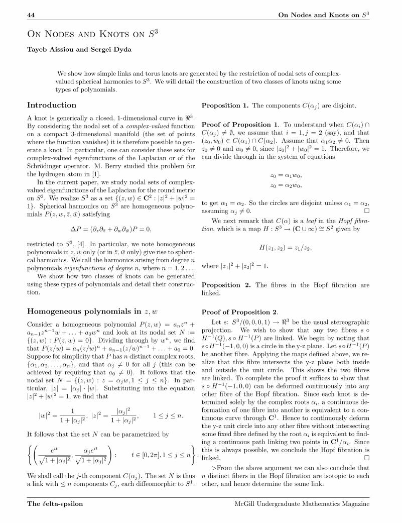
44 On Nodes and Knots on S3
On Nodes and Knots on S3
Tayeb Aissiou and Sergei Dyda
We show how simple links and torus knots are generated by the restriction of nodal sets of complex-valued spherical harmonics to S3. We will detail the construction of two classes of knots using sometypes of polynomials.
Introduction
A knot is generically a closed, 1-dimensional curve in ℜ3.By considering the nodal set of a complex-valued functionon a compact 3-dimensional manifold (the set of pointswhere the function vanishes) it is therefore possible to gen-erate a knot. In particular, one can consider these sets forcomplex-valued eigenfunctions of the Laplacian or of theSchrodinger operator. M. Berry studied this problem forthe hydrogen atom in [1].
In the current paper, we study nodal sets of complex-valued eigenfunctions of the Laplacian for the round metricon S3. We realize S3 as a set (z, w) ∈ C2 : |z|2 + |w|2 =1. Spherical harmonics on S3 are homogeneous polyno-mials P (z, w, z, w) satisfying
∆P = (∂z∂z + ∂w∂w)P = 0,
restricted to S3, [4]. In particular, we note homogeneouspolynomials in z, w only (or in z, w only) give rise to spheri-cal harmonics. We call the harmonics arising from degree npolynomials eigenfunctions of degree n, where n = 1, 2 . . ..
We show how two classes of knots can be generatedusing these types of polynomials and detail their construc-tion.
Homogeneous polynomials in z, w
Consider a homogeneous polynomial P (z, w) = anzn +an−1z
n−1w + . . . + a0wn and look at its nodal set N :=
(z, w) : P (z, w) = 0. Dividing through by wn, we findthat P (z/w) = an(z/w)n + an−1(z/w)n−1 + . . . + a0 = 0.Suppose for simplicity that P has n distinct complex roots,α1, α2, . . . , αn, and that αj 6= 0 for all j (this can beachieved by requiring that a0 6= 0). It follows that thenodal set N = (z, w) : z = αjw, 1 ≤ j ≤ n. In par-ticular, |z| = |αj | · |w|. Substituting into the equation|z|2 + |w|2 = 1, we find that
|w|2 =1
1 + |αj |2, |z|2 =
|αj |21 + |αj |2
, 1 ≤ j ≤ n.
It follows that the set N can be parametrized by
(
eit
√
1 + |αj |2,
αjeit
√
1 + |αj |2
)
: t ∈ [0, 2π], 1 ≤ j ≤ n
.
We shall call the j-th component C(αj). The set N is thusa link with ≤ n components Cj , each diffeomorphic to S1.
Proposition 1. The components C(αj) are disjoint.
Proof of Proposition 1. To understand when C(αi) ∩C(αj) 6= ∅, we assume that i = 1, j = 2 (say), and that(z0, w0) ∈ C(α1) ∩ C(α2). Assume that α1α2 6= 0. Thenz0 6= 0 and w0 6= 0, since |z0|2 + |w0|2 = 1. Therefore, wecan divide through in the system of equations
z0 = α1w0,
z0 = α2w0,
to get α1 = α2. So the circles are disjoint unless α1 = α2,assuming αj 6= 0. ¤
We next remark that C(α) is a leaf in the Hopf fibra-tion, which is a map H : S3 → (C ∪∞) ∼= S2 given by
H(z1, z2) = z1/z2,
where |z1|2 + |z2|2 = 1.
Proposition 2. The fibres in the Hopf fibration arelinked.
Proof of Proposition 2.
Let s: S3/(0, 0, 0, 1) → ℜ3 be the usual stereographicprojection. We wish to show that any two fibres s H−1(Q), s H−1(P ) are linked. We begin by noting thatsH−1(−1, 0, 0) is a circle in the y-z plane. Let sH−1(P )be another fibre. Applying the maps defined above, we re-alize that this fibre intersects the y-z plane both insideand outside the unit circle. This shows the two fibresare linked. To complete the proof it suffices to show thats H−1(−1, 0, 0) can be deformed continuously into anyother fibre of the Hopf fibration. Since each knot is de-termined solely by the complex roots αi, a continuous de-formation of one fibre into another is equivalent to a con-tinuous curve through C1. Hence to continuously deformthe y-z unit circle into any other fibre without intersectingsome fixed fibre defined by the root αi is equivalent to find-ing a continuous path linking two points in C1/αi. Sincethis is always possible, we conclude the Hopf fibration islinked. ¤
>From the above argument we can also conclude thatn distinct fibers in the Hopf fibration are isotopic to eachother, and hence determine the same link.
The δelta-ǫpsilon McGill Undergraduate Mathematics Magazine

On Nodes and Knots on S3 45
Figure 1: Two leafs of the Hopf fibration (links) plottedusing the above construction.
Torus knots
Let m > 1, n > 1, (m,n) = 1 be two relatively prime inte-gers.
Proposition 3. There exist two (real) spherical harmon-ics P,Q on S3 such that the nodal set of P + iQ has con-nected components isomorphic to the (m,n) torus knot.
Proof of Proposition 3. The idea is to choose a real-valued polynomial P (z, z, w, w) that will be “responsible”for rotation around the torus, and real-valued polyno-mial Q(z, z, w, w) that will be “responsible” for localiza-tion on the torus. Then the components of the nodal setN (P + iQ) = N (P ) ∩N (Q) will define the torus knot.
We proceed to choose
P (z, z, w, w) = zmwn + wnzm. (4)
This polynomial is harmonic (since every term is har-monic), and its nodal set is given by
(z/z)m = −(w/w)n.
Letting z = |z|eit, w = |w|eis, we find that
2mt = −π + 2ns ( mod 2π),
so t and s are related by
t =π(2j − 1)
2m+
ns
m,
thus defining the rotation around the torus.We next describe the polynomial Q(z, z, w, w) =
Q(|z|, |w|). According to [3, Thm. 4.1], its restriction to
S3 = |z|2 + |w|2 = 1 is given by the Jacobi polynomialP 0,0
n = Pn (this is the only spherical harmonic invariantunder SO(2) × SO(2) ⊂ SO(4)). The zeros of Pn give riseto the two-dimensional tori in S3, while the polynomial Pdefines the rotation around these tori.
¤
Explicit construction for m + n even
We construct the polynomial Q explicitly in the case whenm + n is even, say m + n = 2k. We look for a polynomialQ of the form
k∑
j=0
ak−j |z|2(k−j)|w|2j .
Setting ak=1 and demanding that Q be harmonic impossesthat
aj = (−1)j
(
k
j
)2
.
Accordingly, if we let |z|2/|w|2 = x, we find that
Q2k = |w|2k
k∑
j=0
(−1)j
(
k
j
)2
xj
:= |w|2kqk(x),
where qk(x) =∑k
j=0(−1)j(
kj
)2xj . Form a related generat-
ing function
qk(x) :=
k∑
j=0
(
k
j
)2
xj .
Claim 1.
qk(x) =
k∑
j=0
(
k
j
)2
xj = (1 − x)kPk((1 + x)/(1 − x)),
where Pk is the k-th Legendre polynomial.
Proof of the Claim: This can be done by induction onk by showing the Legendre polynomial recursion relation
(k + 1) Pk+1(x) − (2k + 1) x Pk(x) + k Pk−1(x) = 0.
is valid. The details are left as an exercise to thereader. ¤
It follows from Claim 1 that
qk(x) = (1 + x)kPk((1 − x)/(1 + x)).
Accordingly, if we let −1 ≤ αk < αk−1 < . . . < α1 < α0 ≤1 denote the roots of Pk(x), then the roots βj of qk(x)satisfy (1 − βj)/(1 + βj) = αj , or
βj =1 − αj
1 + αj.
It follows that all βj are real and positive.
The δelta-ǫpsilon McGill Undergraduate Mathematics Magazine
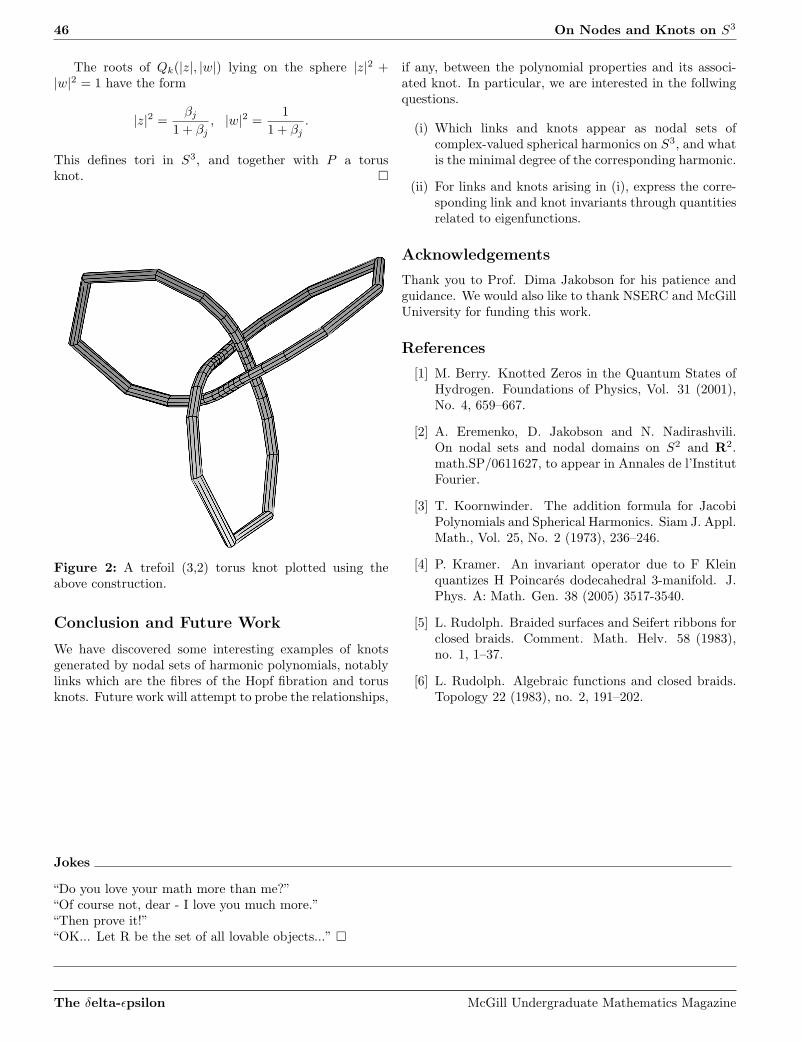
46 On Nodes and Knots on S3
The roots of Qk(|z|, |w|) lying on the sphere |z|2 +|w|2 = 1 have the form
|z|2 =βj
1 + βj, |w|2 =
1
1 + βj.
This defines tori in S3, and together with P a torusknot. ¤
Figure 2: A trefoil (3,2) torus knot plotted using theabove construction.
Conclusion and Future Work
We have discovered some interesting examples of knotsgenerated by nodal sets of harmonic polynomials, notablylinks which are the fibres of the Hopf fibration and torusknots. Future work will attempt to probe the relationships,
if any, between the polynomial properties and its associ-ated knot. In particular, we are interested in the follwingquestions.
(i) Which links and knots appear as nodal sets ofcomplex-valued spherical harmonics on S3, and whatis the minimal degree of the corresponding harmonic.
(ii) For links and knots arising in (i), express the corre-sponding link and knot invariants through quantitiesrelated to eigenfunctions.
Acknowledgements
Thank you to Prof. Dima Jakobson for his patience andguidance. We would also like to thank NSERC and McGillUniversity for funding this work.
References
[1] M. Berry. Knotted Zeros in the Quantum States ofHydrogen. Foundations of Physics, Vol. 31 (2001),No. 4, 659–667.
[2] A. Eremenko, D. Jakobson and N. Nadirashvili.On nodal sets and nodal domains on S2 and R2.math.SP/0611627, to appear in Annales de l’InstitutFourier.
[3] T. Koornwinder. The addition formula for JacobiPolynomials and Spherical Harmonics. Siam J. Appl.Math., Vol. 25, No. 2 (1973), 236–246.
[4] P. Kramer. An invariant operator due to F Kleinquantizes H Poincares dodecahedral 3-manifold. J.Phys. A: Math. Gen. 38 (2005) 3517-3540.
[5] L. Rudolph. Braided surfaces and Seifert ribbons forclosed braids. Comment. Math. Helv. 58 (1983),no. 1, 1–37.
[6] L. Rudolph. Algebraic functions and closed braids.Topology 22 (1983), no. 2, 191–202.
Jokes
“Do you love your math more than me?”“Of course not, dear - I love you much more.”“Then prove it!”“OK... Let R be the set of all lovable objects...” ¤
The δelta-ǫpsilon McGill Undergraduate Mathematics Magazine
A Few Problems in Analytic Number Theory 47
A Few Problems in Analytic Number Theory
Maksym Radziwill
The four problems below belong to a branch of Number theory called Analytic Number Theory.My hope is that they give a glimpse of this beautiful subject.
1. What is the probability that two integers
are coprime?
Suppose your friend picks a very large integer x (say, biggerthan the number of atoms in the universe). You randomlychoose two integers m,n in the interval [1, x]. What is theprobability that (m,n) = 1? As your friend takes x big-ger and bigger this probability will tend to 6/π2. In otherwords:
limx→∞
1
x2
∑
1 ≤ m, n ≤ x(m, n) = 1
1 =6
π2(1)
There is another more leisurely way to state problem 1.Suppose you are placed at the origin of the plane R2. Sup-pose further that at each lattice point of R2 (each exceptthe origin) there is a beautiful girl studying math. Eachis beautiful and different from the others. If you draw asquare with end vertices at (±R,±R) how many distinctgirls inside the square can you see without moving? Clearlynot all of them! If you see the blonde with coordinate (1, 1)you cannot see the brunette with coordinate (2, 2). How-ever, if someone lets R −→ ∞ the percentage of girls inthe square that you (or as a matter of fact anybody elseat the origin) will be able to see, will tend to 6/π2. Now,such a useful thing clearly needs a proof. Here it is.
Proof. We are going to prove (1). The Moebius functionµ is the unique function N −→ C such that for all integersn ∈ N the relation
∑
d|nµ(d) =
1 if n = 10 otherwise
holds. (Dear reader : if you bother, find an explicit formfor µ(n) and note that |µ(n)| ≤ 1 for all n ∈ N. We’ll usethat last relation.) In particular,
∑
d|md|n
µ(d) =
1 if (m,n) = 10 otherwise
for all m,n ∈ N. The above observations gives that
∑
m, n ≤ x(m, n) = 1
1 =∑
m,n≤x
∑
d|md|n
µ(d)
=∑
d≥1
µ(d)∑
m, n ≤ xd|md|n
1
=∑
d≤x
µ(d)
∑
m ≤ xd|m
1
2
(2)
Exactly ⌊x/d⌋ = x/d + O(1) integers m ≤ x are divisibleby d. Therefore (2) becomes
∑
m, n ≤ x(m, n) = 1
1 = x2∑
d≤x
µ(d)
d2+ O
x∑
d≤x
1
d
(3)
Since 1/t is stricly decreasing and continuous, the bound
∑
d≤x
1
d= O
(∫ x
1
dt
t
)
= O (lnx)
holds. We’re almost finished. We want to replace
∑
d≤x
µ(d)
d2by
∞∑
d=1
µ(d)
d2=
1
ζ(2)=
6
π2
By doing so we over/under estimate by
∑
d>x
µ(d)
d2= O
(
∑
d>x
1
d2
)
= O
(∫ ∞
x
dt
t2
)
= O
(
1
x
)
It follows that (3) is equal to 6x2/π2 + O(x ln x). ¤
2. How many squarefree integers ≤ x ?
In some (naive) sense this problem is the “inverse” of prob-lem 3. How would we approach it? Any integer n can bewritten as n = ab2 with a squarefree. Now n = ab2 issquarefree if and only if b = 1. Is the Moebius function ofany help here? Yes. Just remark that, for n = ab2 with asquarefree,
∑
d2|nµ(d) =
∑
d|bµ(d) =
1 if b = 1 (i.e. n ∈ S)0 otherwise
The δelta-ǫpsilon McGill Undergraduate Mathematics Magazine

48 A Few Problems in Analytic Number Theory
where S is the set of squarefree integers. Therefore, thenumber of squarefree integers ≤ x is,
∑
n≤x
∑
d2|nµ(d) =
∑
d≤√x
µ(d)∑
n ≤ xd2|n
1
=∑
d≤√x
µ(d)( x
d2+ O(1)
)
= x∑
d≤√x
µ(d)
d2+ O
(
x1/2)
Again, we want to replace,
∑
d≤√x
µ(d)
d2by
∞∑
d=1
µ(d)
d2=
1
ζ(2)
Doing so, we make an error of
O
∑
d>√
x
1
d2
= O
(∫ ∞
√x
dt
t2
)
= O
(
1√x
)
It follows that the number of squarefree integers less thanx is equal to x/ζ(2) + O
(
x1/2)
.
3. How many powerful integers ≤ x ?
We say that an integer n ∈ N is powerful if all the expo-nents in its prime factorization are greater than 2. Allsquares are powerful. Are there a lot more of power-ful numbers than squares? No. Not even three timesmore. This glorious fact certainly deserves a proof. Toget started: is there an explicit way to write down a pow-erful number? Note that any integer α ≥ 2 can be writtenas 2n+3m with n ≥ 0 and m ∈ 0, 1. Thus, any powerfulnumber can be written as n2m3 with m squarefree. Hence,the number of powerful integers ≤ x is,
∑
n2m3 ≤ xm ∈ S
1 =∑
m ≤ x1/3
m ∈ S
∑
n≤√
x/m3
1 (4)
=√
x∑
m ≤ x1/3
m ∈ S
( √x
m3/2+ O(1)
)
=√
x∑
m ≤ x1/3
m ∈ S
m−3/2 + O(
x1/3)
We use our old trick and replace the finite sum above bythe infinite sum
∑
m∈Sm−3/2 =
ζ (3/2)
ζ (3)
This operation costs
O
∑
m>x1/3
1
m3/2
= O
(∫ ∞
x1/3
dt
t3/2
)
= O(
x−1/6)
We conclude that (4) is equal to(
ζ(3/2)ζ(3)
)
· √x + O(
x1/3)
.
4. How many abelian groups of order ≤ x ?
We will need some heavy machinery for this one! Leta(n) denote the number of abelian groups of order n. Bythe fundamental theorem (for finite abelian groups) weknow that a(·) is (weakly) multiplicative. Moreover forany prime p and exponent α ≥ 0 we have a(pα) = P (α),where P (α) is the number of partitions of α. The numberof partitions of α corresponds to the number of solutionsin N to α = x1 + 2x2 + 3x3 + . . ..
For complex |z| < 1,
∞∑
n=1
P (n)zn =∑
x1,x2,...∈N
zx1+2x2+3x3+...
=
(
∑
x1∈N
zx1
) (
∑
x2∈N
z2x2
)
. . .
=
∞∏
j=1
1
1 − zj
Now, for complex Re s > 1, (the product below is takenover the primes),
∞∑
n=1
a(n)
ns=
∏
p
∞∑
j=0
a(
pj)
pjs
=∏
p
∞∑
j=0
P (j)
(
1
ps
)j
=∏
p
∞∏
j=1
1
1 − p−sj=
∞∏
j=1
ζ (sj)
where in the last line we interchanged the two products.(The motivated reader can check that this is legitimate).Let’s define b(n) such that
∑∞n=1 b(n)n−s = ζ(2s)ζ(3s) . . ..
Thus∑
d|n b(d) = a(n) and
∑
n≤x
|b(n)| = Oε
(
x1/2+ε)
for any fixed ε > 0 (the implicit constant in the big−Odepends on ε). The last estimate is a consequence of the(absolute) convergence of
∑∞n=1 b(n)n−s for all Re s > 1/2.
Now, we are ready to charge. The number of (non-isomorphic, of course) abelian groups of order ≤ x is
∑
n≤x
∑
d|nb(d) =
∑
d≤x
b(d)∑
n ≤ xd|n
1
=∑
d≤x
b(d)(x
d+ O(1)
)
= x∑
d≤x
b(d)
d+ Oε
(
x1/2+ε)
The δelta-ǫpsilon McGill Undergraduate Mathematics Magazine

A Few Problems in Analytic Number Theory 49
We replace the finite sum
∑
d≤x
b(d)
dby
∞∑
d=1
b(d)
d=
∞∏
j=2
ζ(j)
making an error of
O
(
∑
d>x
|b(d)|d
)
= O
(
1
x1/2−ε·∑
d>x
|b(d)|d1/2+ε
)
= O(
x−1/2+ε)
where the last estimate follows from the convergence of∑∞
d=1 |b(d)|d−1/2−ε . We conclude that the number ofabelian groups 6 x is
∞∏
j=2
ζ(j)
· x + Oε
(
x1/2+ε)
With a little more work Erdos and Sarkozy showed that
∑
1≤n≤x
a(n) =
∞∏
j=2
ζ(j)
· x + O(
x1/2)
.
For an more precise estimate, see Ivic’s book.
Concluding remarks
In the end, what is Analytic number theory? The an-swer, if such a thing exists, is approximated by the fol-lowing quote of Henryk Iwaniec (one of the great Analytic
number theorists of this century): “Analytic number theorypursues hard classical problems of an arithmetical natureby means of best available technologies from any branch ofmathematics, and that is its beauty and strength. Analyticnumber theory is not driven by one concept; consequentlyit has no unique identity.”
Let us note that the problems given above, altough nothard (if we are satisfied with the remainder terms as given)and folklore, contains the germs of extremely deep prob-lems. Improving the error term in problem 2, requires theuse of analytical techniques. In fact, establishing a verysharp error term is a problem at the depth of the RiemannHypothesis. The estimates in problems 2, 3 and 4 can allbe improved by the use of complex analysis. (see [2])
It is my hope that the reader perceive a certain coher-ence in the demarche used to solve the above problems,so that Iwaniec’s remark gains in strength. It took me awhile to realize how true and wonderful it is!
References
[1] Edmund Hlawka. Geometric and analytic numbertheory Springer-Verlag, c1991.
[2] Harold Davenport. Multiplicative Number Theory.Springer, third edition, 2000.
[3] Aleksandar Ivic. Lectures on mean values of theRiemann Zeta function Springer-Vlg, c1991.
Jokes
A chemist, a physicist, and a mathematician are stranded on an island when a can of food rolls ashore. The chemistand the physicist comes up with many ingenious ways to open the can. Then suddenly the mathematician gets a brightidea: “Assume we have a can opener ...” ¤
A lecturer: “Now we’ll prove the theorem. In fact I’ll prove it all by myself.” ¤
Q: What does an analytic number theorist say when he’s drowning?A: Log-log, log-log, log... ¤
Q: Why can’t you grow wheat in Z/6Z?A: It’s not a field. ¤
Q: Why is the integral along the contour of Western Europe zero?A: Because all the Poles are in the Eastern part. ¤
What is the difference between an argument and a proof? An argument will convince a reasonable man, but a proofis needed to convince an unreasonable one. ¤
The δelta-ǫpsilon McGill Undergraduate Mathematics Magazine

50 Graduate Studies: Applications and Beyond
Graduate Studies: Applications and Beyond
Leonid Chindelevitch
Those of you who are entering your last year of undergraduate studies are probably consideringdifferent options for what lies ahead. Those of you who still have a year or two to go may not be soworried yet, but nevertheless the question of where to go next invariably comes to mind from timeto time. And when you are dealing with existential questions of this kind, it always helps to knowthat you are not alone, and that other people have gone through the same ordeal.
Since enrolling in graduate school is certainly one of themost popular options, In this short article I am going toanswer some questions that you will undoubtedly be ask-ing yourselves when the time comes to apply to graduateschool. My hope is that it will help you avoid some of thedifficulties that I had to face at this time two years ago.
But first, some background questions to give you anidea of where I am coming from.
What did you do in undergrad? I was a McGillundergraduate student in the Joint Honours program inMathematics and Computer Science from 2003 to 2006.What convinced me to go on to graduate school were mythree successful NSERC-USRA summer research experi-ences.
What university are you currently enrolled in? Iam starting the second year of a PhD program in AppliedMathematics at MIT (Massachusetts Institute of Technol-ogy - if you apply there, make sure you get the name right).That’s in the U.S., but only a 5-6 hour drive away fromMontreal.
What are you specializing in? My areas of applica-tion are biology and linguistics. This is a little bit unusual(the “standard”areas of application for mathematics beingphysics, computer science, and combinatorics), but that iswhat matches my research interests.
What are the good schools in your field of stud-ies? Generally speaking, there are a lot of excellent uni-versities in Canada and the United States, in both pureand applied mathematics. In Canada, McGill, Universityof Toronto and University of British Columbia are particu-larly strong in mathematics (both pure and applied), whileWaterloo and Simon Fraser University are very strong inapplied mathematics. In the US, the top universities forpure math would be Harvard, MIT, Princeton, Berkeleyand Stanford; for applied math: MIT, New York Univer-sity, Berkeley, Brown, Johns Hopkins, and I am certainlyforgetting some others. You can consult the latest an-nual ratings available at the Careers and Placement Center(CAPS), located in the Brown building. I also used their
help to improve my personal statement (it’s a free service,so take advantage of it)!
When did you first think about where you wantedto go? I believe that I first heard about MIT in my firstyear of undergrad. The context was that it’s a well-reputedschool which is very difficult to get in. It was at that timethat I decided to make it a challenge for myself to get intograduate school there. I like setting high goals, although Ididn’t believe I could achieve this one until I actually gotmy acceptance letter.
When should we start thinking about it? It’s nevertoo early to start thinking about where you would like togo. However, you should definitely start planning your ap-plication process in September of your last year. If youwait longer, things may get difficult (especially if you areapplying to universities in the US). Also, make sure toapply for funding before the deadlines in mid-October!
And now, the questions which are directly related tothe application process. I would like to mention that myfriend Marco Carone, whose story is similar to mine, haswritten an excellent and very detailed overview of the ap-plication process, which is available online2.
When should we start applying? Different universi-ties have different deadlines. If you are going to be apply-ing to US universities, their deadlines are earlier (typicallyaround mid-December). Canadian universities have laterdeadlines (usually February or March), but if you can getall of your applications out of the way before Christmasbreak, you will save yourself a lot of time in your lastsemester. I did everything just before the deadlines, butin retrospective, I wish I hadn’t.
How much time does it take to apply? This dependson the number of universities you apply to. I applied tosix (and I wouldn’t recommend applying to more than 10).The first application is always the hardest. The statementof purpose, the biographical information, the reference let-ters, the GRE scores, the textbook information - believe itor not, some schools actually ask you to list all the text-books you have used during your undergraduate career - allthese take a long time to put together. Each subsequent
2www.math.mcgill.ca/students/undergrad/gradschoolapp
The δelta-ǫpsilon McGill Undergraduate Mathematics Magazine

Graduate Studies: Applications and Beyond 51
one gets easier, but it is still a considerable time invest-ment. On average, I would estimate about 5-10 hours peruniversity (extended over a period of several days, becauseof all the different components).
Finally, some questions related to graduate studies ingeneral, and PhD studies in the US in particular.
How does one pay for one’s graduate studies? Usu-ally, the university will mention the conditions of your ad-mission in your acceptance letter; in particular, you will benotified about the source of funding for your studies. Typi-cally, your tuition will be free (covered by the department);you will also receive some money for living expenses. Inexchange, the university will usually impose some teachingduties on you, such as grading papers or teaching a sec-tion in one of the undergraduate courses. Since grading isnot as much fun as teaching, make sure to find out whatrequirements you need to fulfill to get to teach.
Also, you may or may not be able to take the fundingthat you receive from NSERC abroad (FQRNT is usuallymore flexible in that respect); you may also have to ne-gotiate with your university. Some universities will allowyou to combine external funding with departmental fund-ing, some will not (in order to ensure everyone is at thesame level); still others (like MIT) will settle on a compro-mise (e.g. a lower departmental funding plus your externalfunding).
What’s more important in considerering a gradschool: good researchers, good teaching, good gradstudents? One of my friends (a professor) once told methat, although you learn a lot from your teachers, youlearn even more from your peers. Of course, in the idealworld, you would have everything - great students, greatprofessors and exciting research. In reality, there may bea slight trade-off. My suggestion is to visit all the uni-versities where you have been accepted and that you areconsidering (they will usually pay for your travel expenses,even the US ones) and talk to both the professors that youare interested in and to the students. Most importantly,you have to be in an environment which stimulates you,and you are the only one who can decide that. Don’t takeother peoples’ word for it!
What are the pros and cons of doing a PhD withoutdoing a Masters? If you are sure that a PhD is whatyou ultimately want, then going into a PhD program di-rectly (which is what usually happens in the US) is a goodoption. Despite the common misconception, a PhD doesnot mean you have to continue in academia afterwards -it actually gives you a lot of options. The disadvantage isthat you have to go all the way, as you may not get anydiploma otherwise (in a way, you can think of a Mastersdegree as a safety net for that case). Many universities (in-cluding MIT) have so-called “qualifying exams”, and if youfail them twice, you leave without a degree; my qualifyingexams are coming up in two weeks, so I really shouldn’tbe writing this right now... oh well.
On the other hand, if your research background is notas strong as you would like it to be, or if you are not surethat you would like to go all the way to a PhD, then doinga Masters degree first is preferable. This is what typicallyhappens in Canadian universities (although you can get aMasters degree in some US universities too). The disad-vantage is that overall, it may take a year longer to getyour PhD if you go through the Masters program first.
What kind of undergraduate students are fit for aPhD in mathematics? That’s a provocative question!As the goal of most PhD programs is to produce originalresearch (whether in the form of a thesis or otherwise),the most important “fitness” criterion is an interest and anability to do research. The other qualities you will needare perseverance, patience and a willingness to work longhours when necessary; if you do not mind spending severalhours on a challenging assignment problem, then you arean excellent PhD candidate.
Are extracurricular activities important to get ac-cepted in mathematics? Unfortunately, I don’t know.I am still not sure what it was in my resume that got mein, but I am certain that my involvement in extracurricularactivities did not hinder my cause (I was actively involvedin the SUMS council, was the president of the 2006 CUMC,and also ran or helped run several student organizations).From what I understand, the universities look most of allat your research ability, but it also helps if you show youare a “well-rounded” person.
Compare MIT students with McGill students. Ihaven’t talked to enough graduate students at McGill toget a representative sample. The main difference betweenthe undergraduates at McGill and those at MIT is thatthose at McGill actually sleep...
Are you as involved in the MIT student life as youwere here? Unfortunately, not as much, but it’s not forlack of opportunity. I am involved in a lot of extracurric-ular activities and clubs, but mostly as an active memberrather than an executive (with the exception of the MITEsperanto Club).
How was the transition from the Canadian to theAmerican education system? Relatively smooth - theone thing that really gets on my nerves is the use of the im-perial system in the US. From the experience of my friendswho are doing graduate studies in Canada, I would say thatthe difference between undergrad and graduate school ismore significant than the difference between the Canadianand the American education systems.
What’s the meaning of life? The meaning of life isto find the meaning of life! Sorry about the infinite recur-sion...
The δelta-ǫpsilon McGill Undergraduate Mathematics Magazine

52 Credits
Credits
The Delta-Epsilon Editing Team
In alphabetical order
• Agnes F. Beaudry
• Ioan Filip
• Michael McBreen
• Alexandra Ortan
• Vincent Quenneville-Belair
• Nan Yang
Cover Art and Design
• Michael McBreen
• Mathieu Menard
Acknowledgements
Now has come the time to say some thanks! We would like to thank professor Eyal Goren, professor Benoit Charbonneauand Leonid Chindelevitch for taking the time to speak with us and for all the great advice they sent out to theundergraduates. Thank you SUMS for your multi-dimensional support; if it would be as elegant, we truly believe thatyou would give us infinitely many parameters to work with. We are grateful to the Science Undergraduate Society,the Arts Undergraduate Society, the Faculty of Science, the Department of Mathematics and Statistics, the Institutdes sciences mathematiques and the Centre de recherche mathematiques for providing the funding. We also take thisoccasion to thank the Science Undegraduate Society for awarding us the Best Student Publication Award for last year’sissue. We also would like to thank Alex Dergachev for having freely let us use his server without which editing a journalis a mess. Finally, thank you, reader, for the thing you are defined to do! Without you, needless to say, we would beuseless.
The δelta-ǫpsilon McGill Undergraduate Mathematics Magazine


