The Demonstrations & Science Experiment (DSX) Experiment (DSX) Update for RBSP Science Working Group 23-24 May 2011 Dave Lauben, Stanford Gregory Ginet, MIT/LL Michael Starks, AFRL Mark Scherbarth, AFRL
Transcript
The Demonstrations & Science Experiment (DSX)Experiment (DSX)
Update for RBSP Science Working Group
23-24 May 2011
Dave Lauben, Stanford Gregory Ginet, MIT/LLMichael Starks, AFRLMark Scherbarth, AFRL
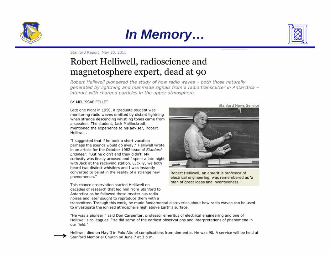
In Memory…
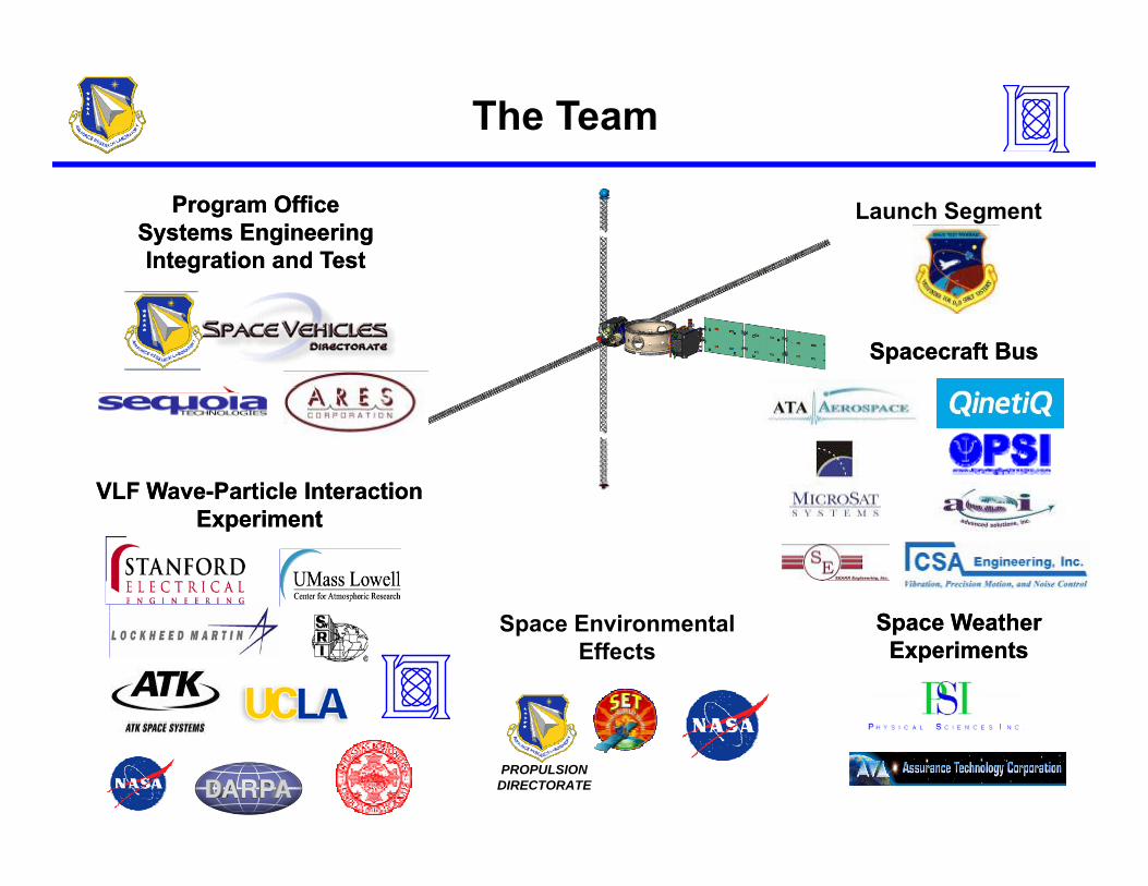
The Team
Launch SegmentProgram OfficeProgram OfficeSystems EngineeringSystems EngineeringIntegration and TestIntegration and Test
Spacecraft BusSpacecraft Bus
VLF WaveVLF Wave--Particle Interaction Particle Interaction a ea e a t c e te act oa t c e te act oExperimentExperiment
Space EnvironmentalEffects
Space WeatherSpace WeatherExperimentsExperiments
PROPULSIONDIRECTORATE
Outline
• Introduction and Motivation• DSX spacecraft and experimental payloads• Science question where is the 20 dB?• Science question – where is the 20 dB?• Science question – radiation pattern in plasma?• Conjunction opportunities• Summary
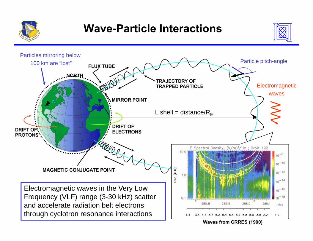
Wave-Particle Interactions
Particles mirroring below 100 km are “lost” Particle pitch-angle
ELF/VLF Waves Control Particle Lifetimes Electromagnetic waves
L shell = distance/RE
Electromagnetic waves in the Very Low Frequency (VLF) range (3 30 kHz) scatterFrequency (VLF) range (3-30 kHz) scatter and accelerate radiation belt electrons through cyclotron resonance interactions
Waves from CRRES (1990)
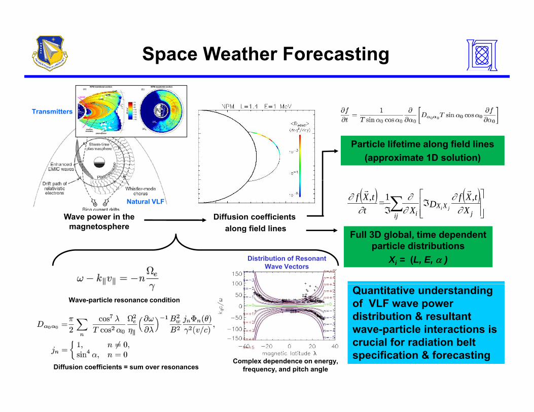
Space Weather Forecasting
Transmitters
Diffusion coefficient along field lines
Particle lifetime along field lines(approximate 1D solution)
Wave power in the magnetosphere
Diffusion coefficients along field lines
( ) ( )⎥⎥⎦
⎤
⎢⎢⎣
⎡ℑ
ℑ∑ jXX
iijX
tXfD
X=
ttXf
ji ∂∂
∂∂
∂∂ ,1,
F ll 3D l b l ti d d t
Natural VLF
gFull 3D global, time dependent
particle distributions Xi = (L, E, α )Distribution of Resonant
Wave Vectors
Quantitative understanding of VLF wave power distribution & resultant wave-particle interactions is
Wave-particle resonance condition
crucial for radiation belt specification & forecasting
Diffusion coefficients = sum over resonancesComplex dependence on energy,
frequency, and pitch angle
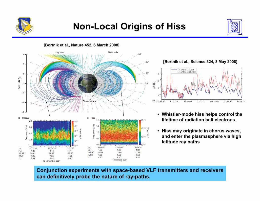
Non-Local Origins of Hiss
[Bortnik et al., Nature 452, 6 March 2008]
[Bortnik et al., Science 324, 8 May 2008][Bortnik et al., Science 324, 8 May 2008]
Whi tl d hi h l t l th• Whistler-mode hiss helps control the lifetime of radiation belt electrons.
• Hiss may originate in chorus waves, and enter the plasmasphere via high p p glatitude ray paths
Conjunction experiments with space-based VLF transmitters and receivers can definitively probe the nature of ray-paths.
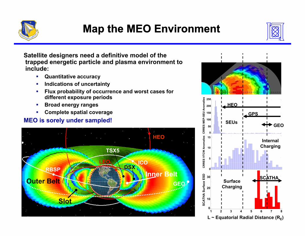
Map the MEO EnvironmentMap the MEO Environment
Satellite designers need a definitive model of the trapped energetic particle and plasma environment to include:
Slot (Dose behind 82.5 mils Al)
Quantitative accuracyIndications of uncertaintyFlux probability of occurrence and worst cases for different exposure periodsB d HEO
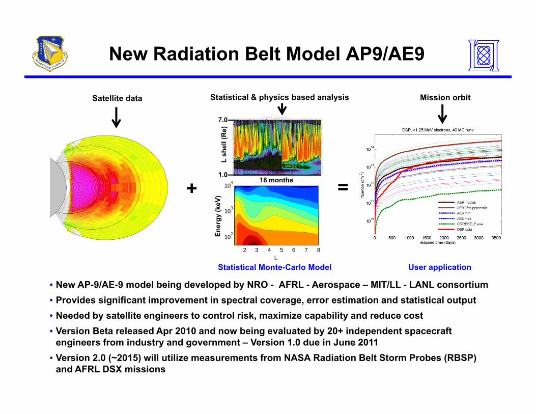
Satellite data Statistical & physics based analysis Mission orbit
TEM1c PC 4 (6.77%)4 18 months
L sh
ell (
Re
1.0
Ener
gy (k
eV)
( %)
2
103
104 18 months+ =E
L
2 3 4 5 6 7 8
102
Statistical Monte-Carlo Model User application
• New AP-9/AE-9 model being developed by NRO - AFRL - Aerospace – MIT/LL - LANL consortium• New AP-9/AE-9 model being developed by NRO - AFRL - Aerospace – MIT/LL - LANL consortium• Provides significant improvement in spectral coverage, error estimation and statistical output• Needed by satellite engineers to control risk, maximize capability and reduce cost • Version Beta released Apr 2010 and now being evaluated by 20+ independent spacecraft
engineers from industry and government – Version 1.0 due in June 2011• Version 2.0 (~2015) will utilize measurements from NASA Radiation Belt Storm Probes (RBSP)
and AFRL DSX missions
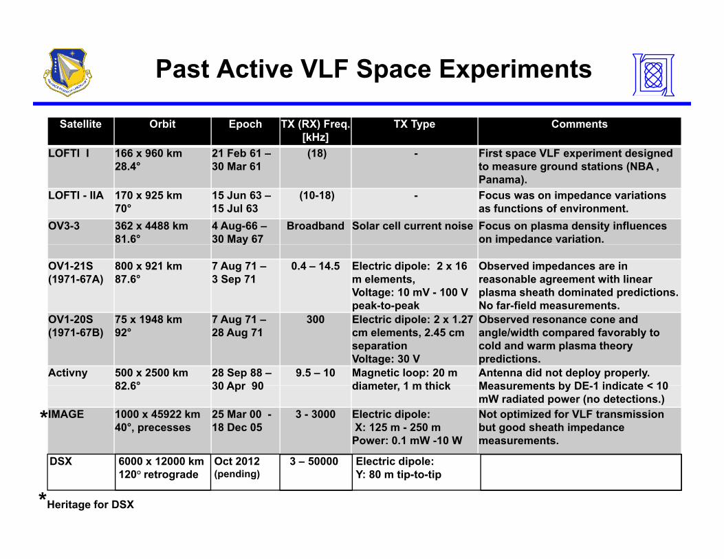
Past Active VLF Space Experiments
Satellite Orbit Epoch TX (RX) Freq. [kHz]
TX Type Comments
LOFTI I 166 x 960 km28.4°
21 Feb 61 –30 Mar 61
(18) - First space VLF experiment designed to measure ground stations (NBA ,Panama).
LOFTI - IIA 170 x 925 km70°
15 Jun 63 –15 Jul 63
(10-18) - Focus was on impedance variations as functions of environment.
OV3-3 362 x 4488 km81.6°
4 Aug-66 –30 May 67
Broadband Solar cell current noise Focus on plasma density influences on impedance variation.y p
OV1-21S (1971-67A)
800 x 921 km87.6°
7 Aug 71 –3 Sep 71
0.4 – 14.5 Electric dipole: 2 x 16 m elements, Voltage: 10 mV - 100 V peak-to-peak
Observed impedances are in reasonable agreement with linearplasma sheath dominated predictions. No far-field measurements.
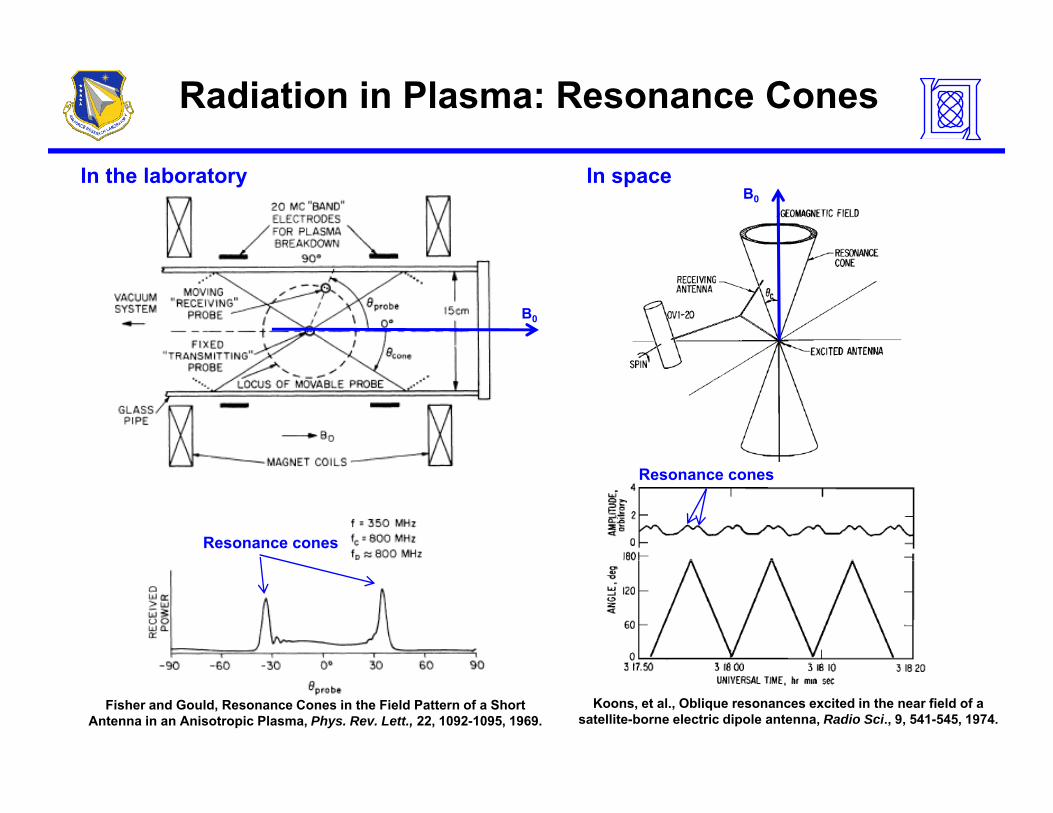
OV1-20S (1971-67B)
75 x 1948 km92°
7 Aug 71 –28 Aug 71
300 Electric dipole: 2 x 1.27 cm elements, 2.45 cm separationVoltage: 30 V
Observed resonance cone and angle/width compared favorably to cold and warm plasma theory predictions.
Activny 500 x 2500 km82 6°
28 Sep 88 –30 Apr 90
9.5 – 10 Magnetic loop: 20 m diameter 1 m thick
Antenna did not deploy properly. Measurements by DE 1 indicate < 1082.6 30 Apr 90 diameter, 1 m thick Measurements by DE-1 indicate < 10 mW radiated power (no detections.)
IMAGE 1000 x 45922 km40°, precesses
25 Mar 00 -18 Dec 05
3 - 3000 Electric dipole:X: 125 m - 250 m Power: 0.1 mW -10 W
Not optimized for VLF transmission but good sheath impedance measurements.
*
*Heritage for DSX
DSX 6000 x 12000 km120° retrograde
Oct 2012(pending)
3 – 50000 Electric dipole:Y: 80 m tip-to-tip
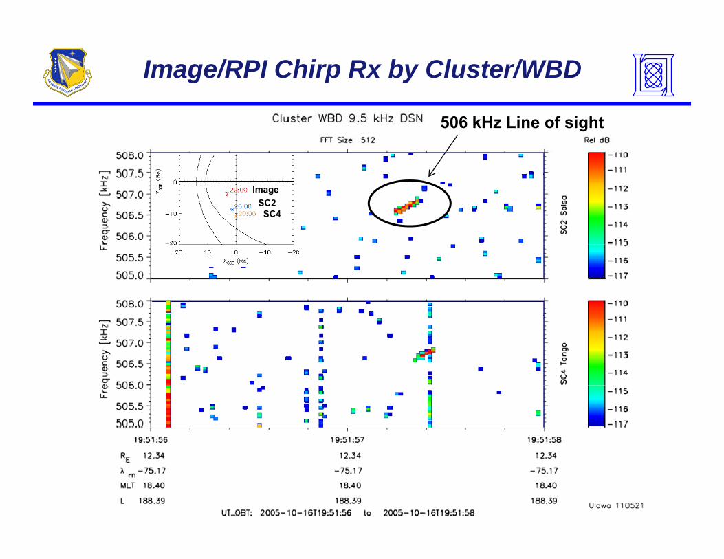
Image/RPI Chirp Rx by Cluster/WBD
506 kHz Line of sight
ImageSC2SC4
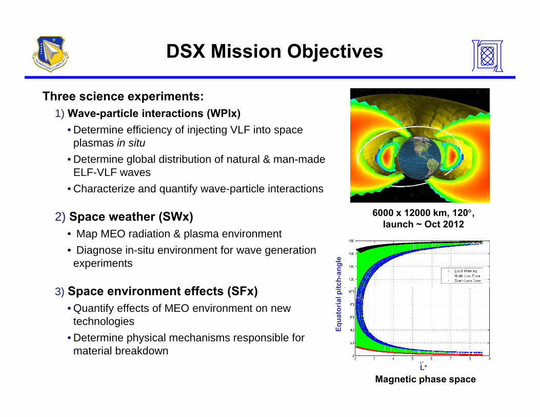
DSX Mission Objectives
Three science experiments:1) Wave-particle interactions (WPIx)
• Determine efficiency of injecting VLF into space• Determine efficiency of injecting VLF into space plasmas in situ
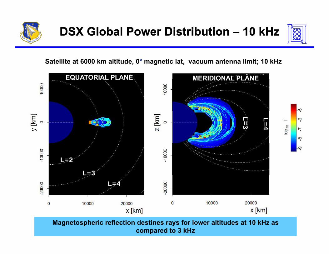
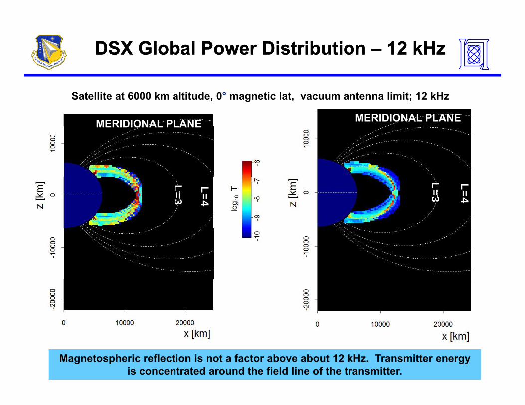
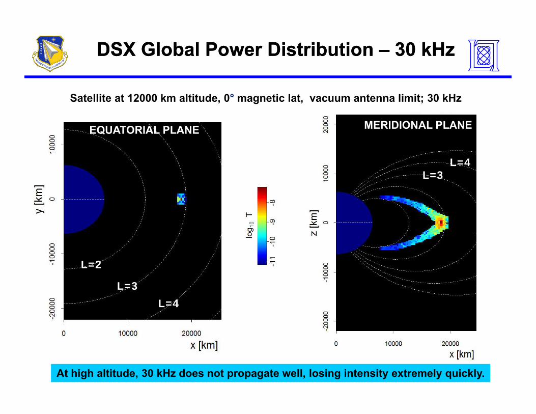
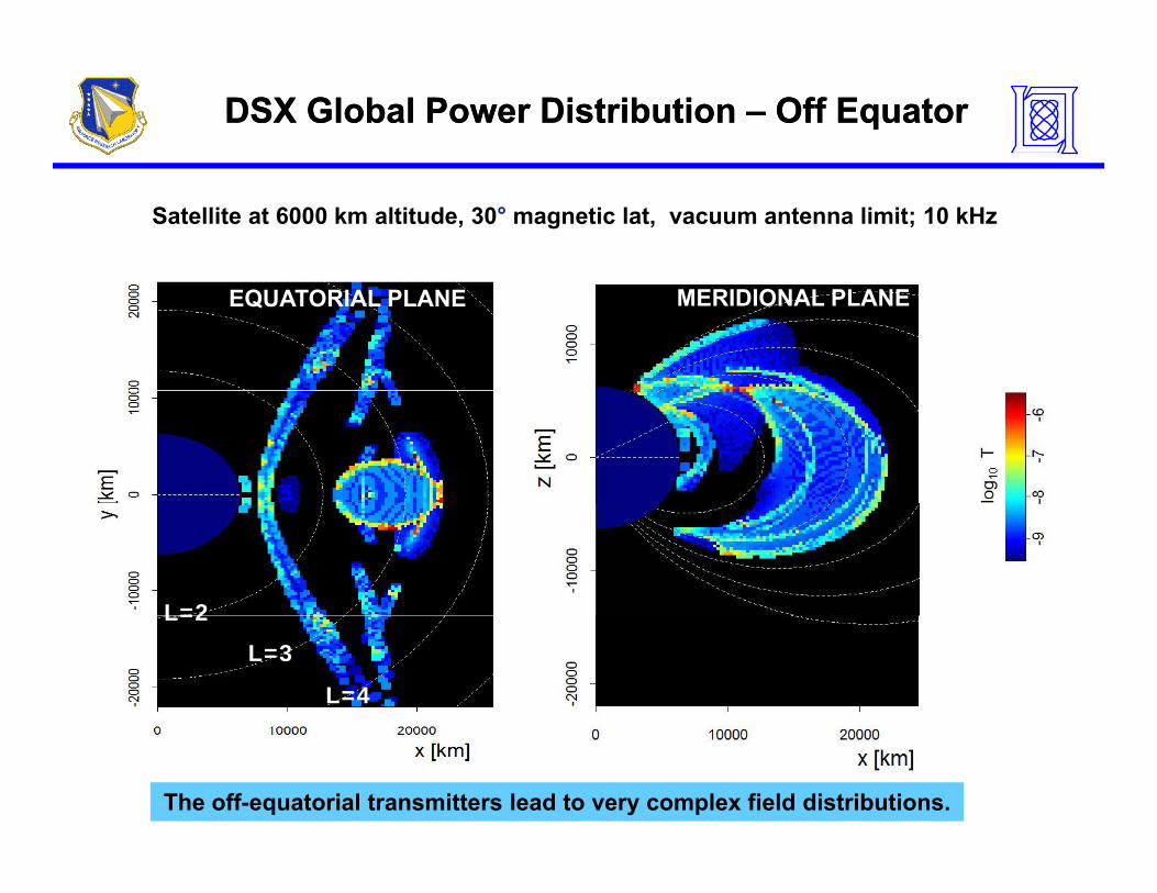
• Determine global distribution of natural & man-made ELF-VLF waves
• Characterize and quantify wave-particle interactions
2) Space weather (SWx)• Map MEO radiation & plasma environment
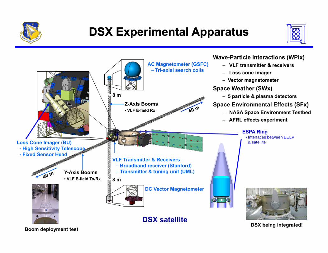
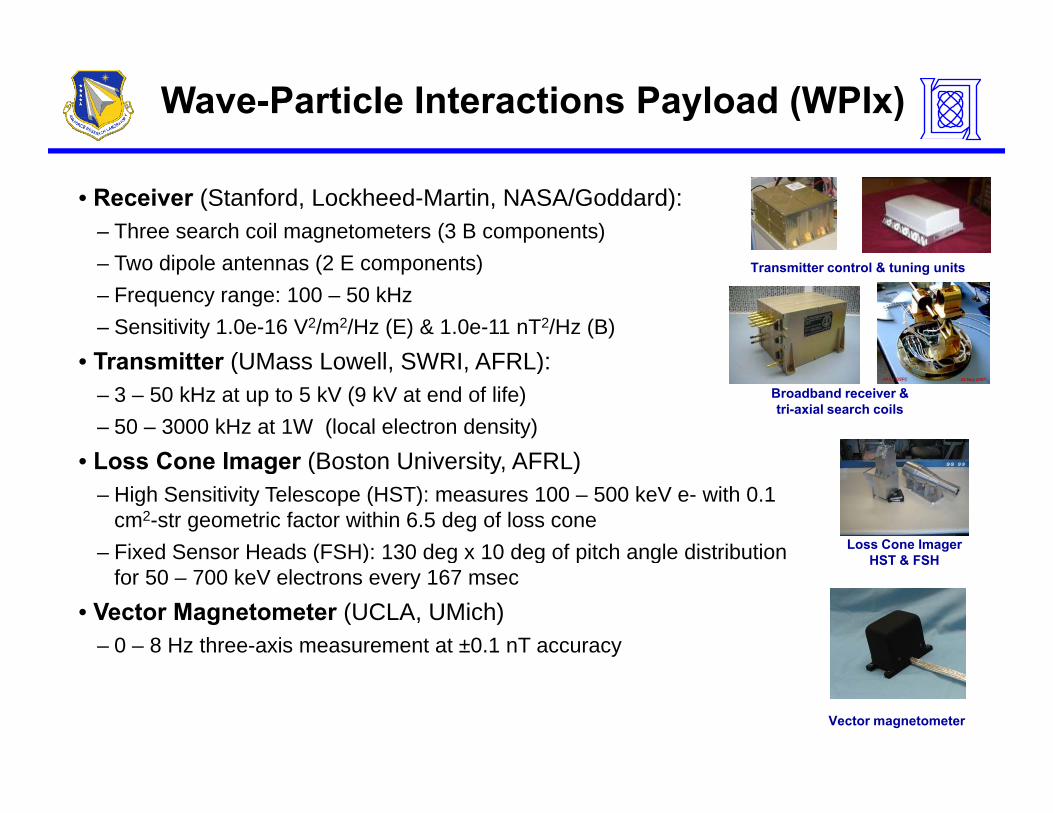
• Receiver (Stanford, Lockheed-Martin, NASA/Goddard):– Three search coil magnetometers (3 B components)– Two dipole antennas (2 E components)– Frequency range: 100 – 50 kHz – Sensitivity 1.0e-16 V2/m2/Hz (E) & 1.0e-11 nT2/Hz (B) T itt (UM L ll SWRI AFRL)
Transmitter control & tuning units
• Transmitter (UMass Lowell, SWRI, AFRL):– 3 – 50 kHz at up to 5 kV (9 kV at end of life)– 50 – 3000 kHz at 1W (local electron density)
• Loss Cone Imager (Boston University AFRL)
Broadband receiver & tri-axial search coils
14 May 2007NASA GSFC 14 May 200714 May 2007NASA GSFC
• Loss Cone Imager (Boston University, AFRL)– High Sensitivity Telescope (HST): measures 100 – 500 keV e- with 0.1
cm2-str geometric factor within 6.5 deg of loss cone– Fixed Sensor Heads (FSH): 130 deg x 10 deg of pitch angle distribution Loss Cone Imager
HST & FSH( ) g g p gfor 50 – 700 keV electrons every 167 msec
• Vector Magnetometer (UCLA, UMich)– 0 – 8 Hz three-axis measurement at ±0.1 nT accuracy
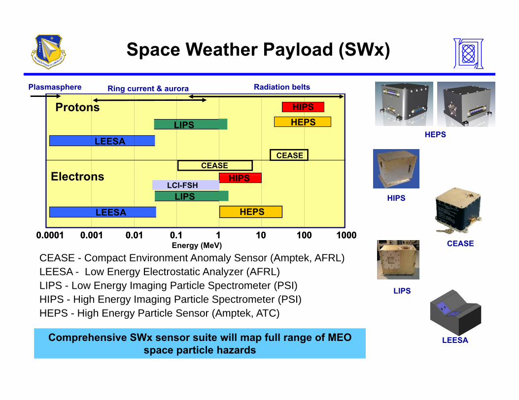
gy y ( )LIPS - Low Energy Imaging Particle Spectrometer (PSI)HIPS - High Energy Imaging Particle Spectrometer (PSI)HEPS - High Energy Particle Sensor (Amptek, ATC)
LIPS
Comprehensive SWx sensor suite will map full range of MEO space particle hazards
Comprehensive SWx sensor suite will map full range of MEO space particle hazards
LEESA
Space Weather Effects Payload (SFx)
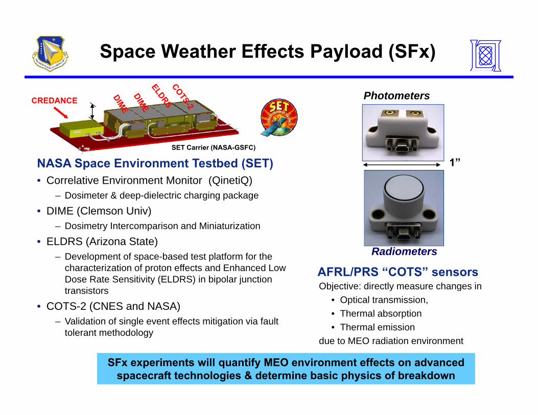
CREDANCE Photometers
SET Carrier (NASA-GSFC)
NASA Space Environment Testbed (SET)• Correlative Environment Monitor (QinetiQ)
1”• Correlative Environment Monitor (QinetiQ)
– Dosimeter & deep-dielectric charging package
• DIME (Clemson Univ)– Dosimetry Intercomparison and Miniaturization
• ELDRS (Arizona State)– Development of space-based test platform for the
characterization of proton effects and Enhanced Low Dose Rate Sensitivity (ELDRS) in bipolar junction
AFRL/PRS “COTS” sensorsRadiometers
Objective: directly measure changes intransistors
• COTS-2 (CNES and NASA)– Validation of single event effects mitigation via fault
SFx experiments will quantify MEO environment effects on advanced spacecraft technologies & determine basic physics of breakdown
SFx experiments will quantify MEO environment effects on advanced spacecraft technologies & determine basic physics of breakdown
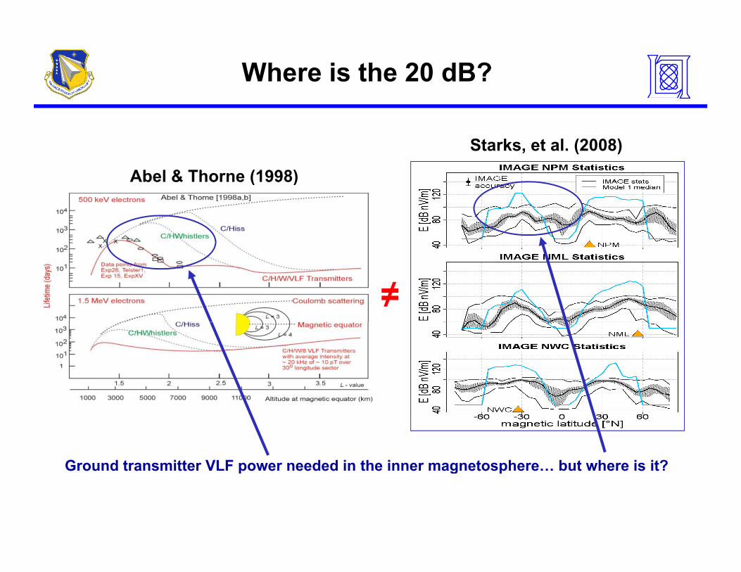
Where is the 20 dB?
Abel & Thorne (1998)
Starks, et al. (2008)
Abel & Thorne (1998)
≠
Ground transmitter VLF power needed in the inner magnetosphere but where is it?Ground transmitter VLF power needed in the inner magnetosphere… but where is it?
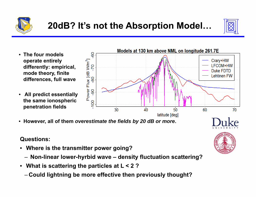
20dB? It’s not the Absorption Model…
• The four models operate entirelyoperate entirely differently: empirical, mode theory, finite differences, full wave
• All predict essentially the same ionospheric penetration fields
• However, all of them overestimate the fields by 20 dB or more.
Questions:• Where is the transmitter power going?
– Non-linear lower-hyrbid wave – density fluctuation scattering?• What is scattering the particles at L < 2 ?
– Could lightning be more effective then previously thought?
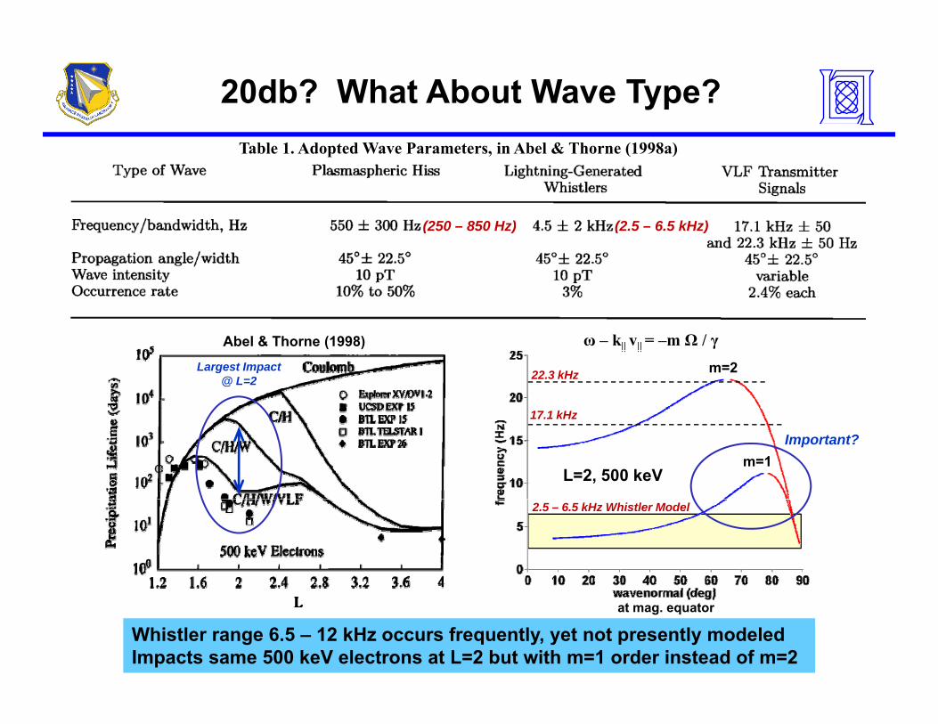
20db? What About Wave Type?
(250 850 Hz) (2 5 6 5 kHz)
Table 1. Adopted Wave Parameters, in Abel & Thorne (1998a)
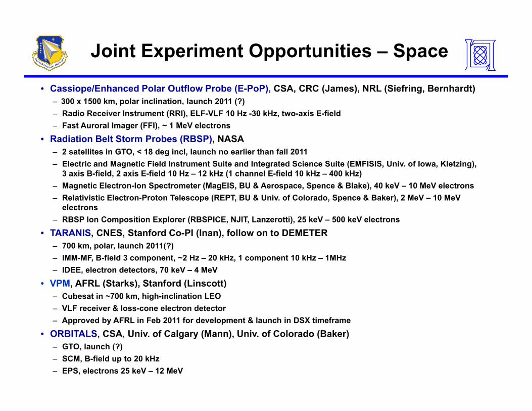
• Radiation Belt Storm Probes (RBSP), NASA– 2 satellites in GTO, < 18 deg incl, launch no earlier than fall 2011– Electric and Magnetic Field Instrument Suite and Integrated Science Suite (EMFISIS, Univ. of Iowa, Kletzing),
electrons– RBSP Ion Composition Explorer (RBSPICE, NJIT, Lanzerotti), 25 keV – 500 keV electrons
TARANIS CNES Stanford Co PI (Inan) follow on to DEMETER• TARANIS, CNES, Stanford Co-PI (Inan), follow on to DEMETER– 700 km, polar, launch 2011(?)– IMM-MF, B-field 3 component, ~2 Hz – 20 kHz, 1 component 10 kHz – 1MHz– IDEE, electron detectors, 70 keV – 4 MeV
• VPM AFRL (Starks) Stanford (Linscott)• VPM, AFRL (Starks), Stanford (Linscott)– Cubesat in ~700 km, high-inclination LEO– VLF receiver & loss-cone electron detector– Approved by AFRL in Feb 2011 for development & launch in DSX timeframe
• ORBITALS CSA Univ of Calgary (Mann) Univ of Colorado (Baker)ORBITALS, CSA, Univ. of Calgary (Mann), Univ. of Colorado (Baker)– GTO, launch (?)– SCM, B-field up to 20 kHz– EPS, electrons 25 keV – 12 MeV
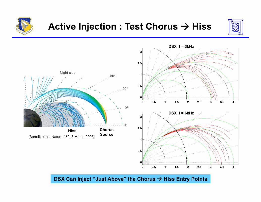
Active Injection : Test Chorus Hiss
DSX f = 3kHz
DSX f = 6kHz
[Bortnik et al., Nature 452, 6 March 2008]
ChorusSource
Hiss
DSX f 6kHz
DSX Can Inject “Just Above” the Chorus Hiss Entry Points
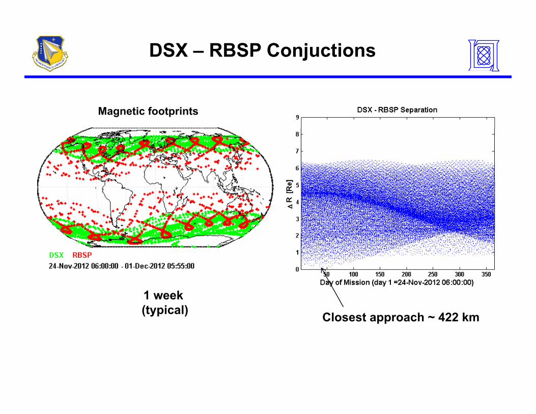
DSX – RBSP Conjuctions
Magnetic footprints
1 week (typical) Closest approach ~ 422 km
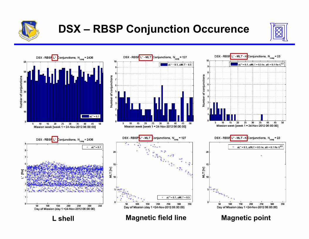
DSX – RBSP Conjunction Occurence
L shell Magnetic field line Magnetic point
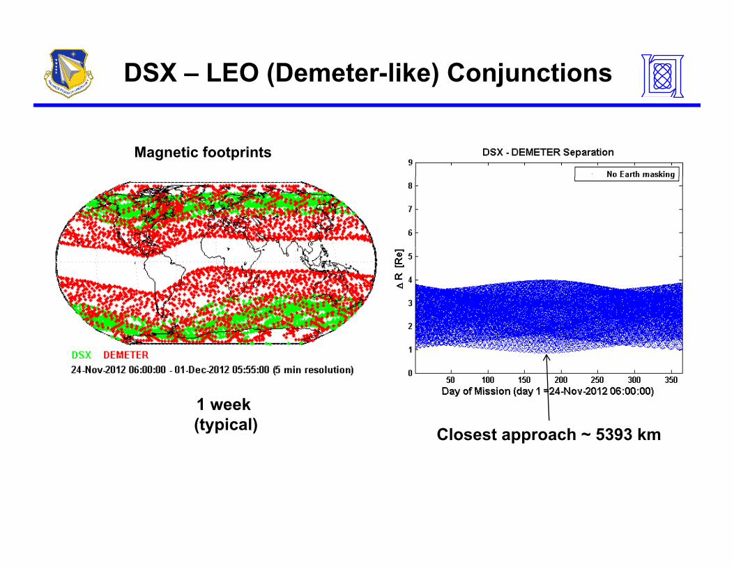
DSX – LEO (Demeter-like) Conjunctions
Magnetic footprints
1 week (typical) Closest approach ~ 5393 km
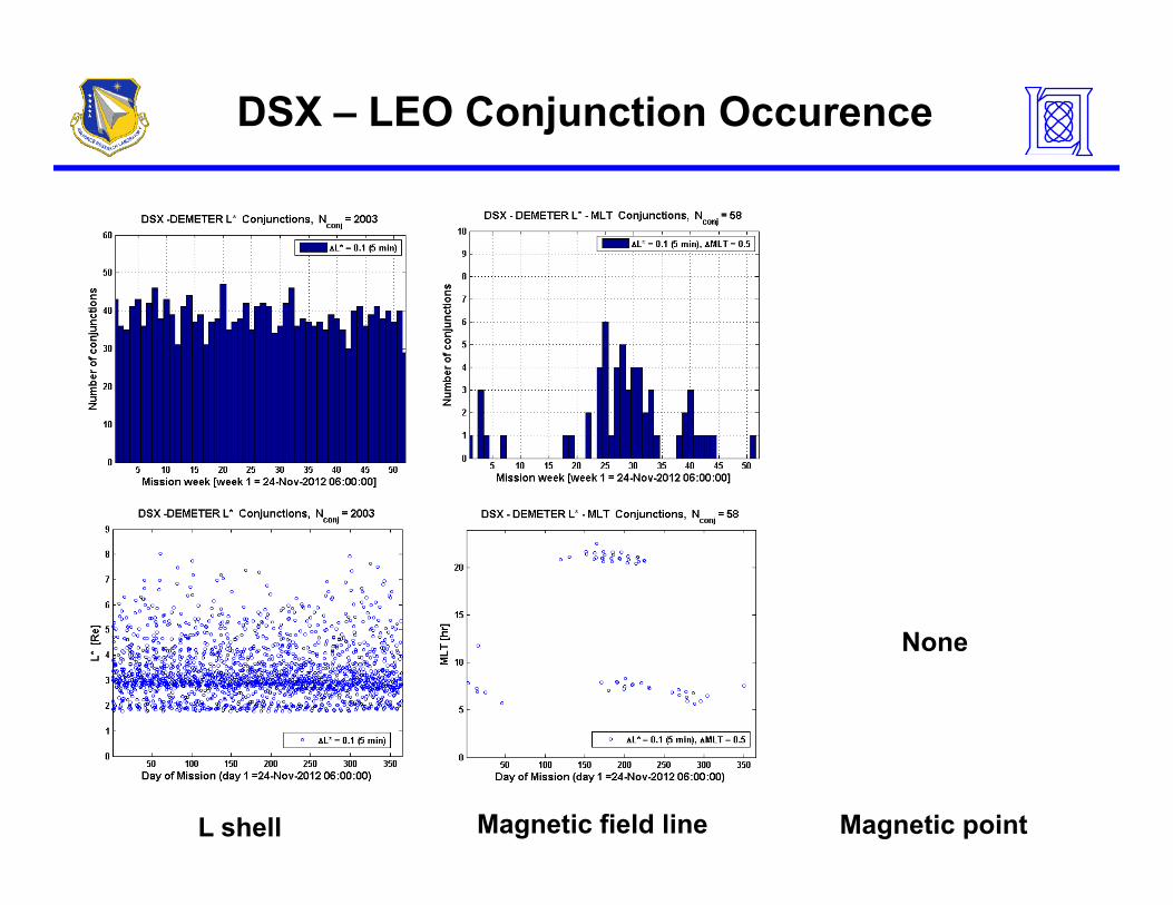
DSX – LEO Conjunction Occurence
None
L shell Magnetic field line Magnetic point
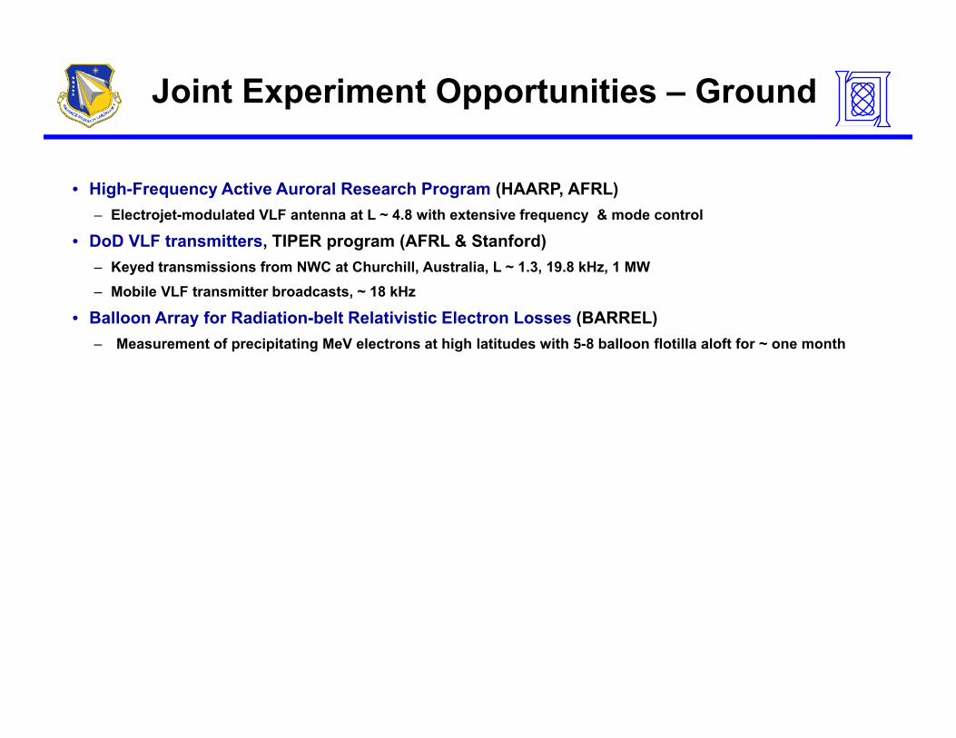
Joint Experiment Opportunities – Ground
• High-Frequency Active Auroral Research Program (HAARP, AFRL)– Electrojet-modulated VLF antenna at L ~ 4.8 with extensive frequency & mode control
• DoD VLF transmitters, TIPER program (AFRL & Stanford)– Keyed transmissions from NWC at Churchill, Australia, L ~ 1.3, 19.8 kHz, 1 MW– Mobile VLF transmitter broadcasts, ~ 18 kHz
• Balloon Array for Radiation-belt Relativistic Electron Losses (BARREL)Balloon Array for Radiation belt Relativistic Electron Losses (BARREL)– Measurement of precipitating MeV electrons at high latitudes with 5-8 balloon flotilla aloft for ~ one month
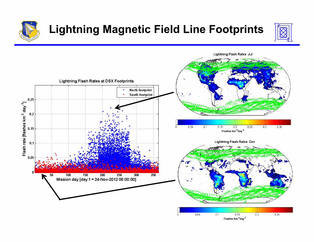
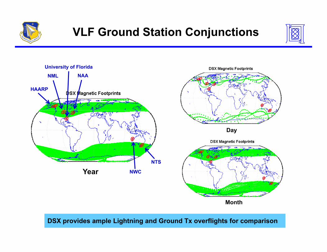
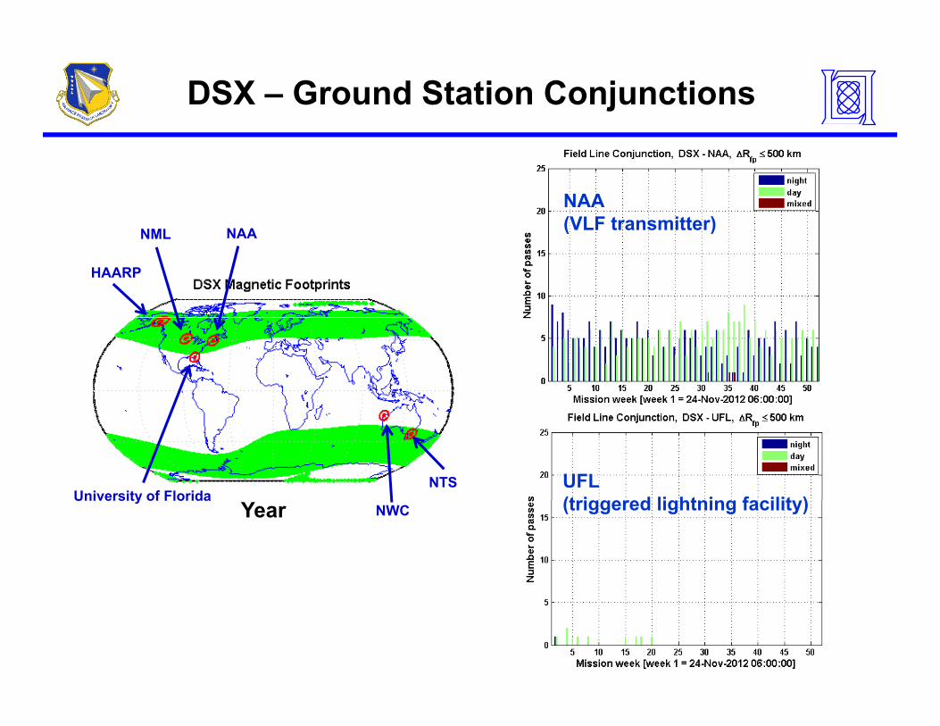
DSX – Ground Station Conjunctions
NAA(VLF transmitter)NAA
HAARP
NML (VLF transmitter)
University of FloridaNTS UFL
(triggered lightning facility)YearUniversity of Florida
NWC (triggered lightning facility)
Summary
• DSX is manifest for launch as secondary payload on DMSP F-19 with launch in Oct 2012 (decision on launch date to be made in Jun 2011)
• DSX will make detailed measurements of in-situ VLF waves– Missing 20 dB of VLF power is a big inner magnetosphere questiong p g g p q
• Tremendous opportunities for mono-static and bi-static VLF transmit-receive measurements
– Determine VLF antenna transmission efficiencyDetermine VLF antenna transmission efficiency – Validate chorus – hiss conversion model
• Comprehensive particle detector suite will map poorly explored MEO regionMEO region
– Provides much needed data to update climatological radiation belt models used for spacecraft design
• Lots of good science to be done!• Lots of good science to be done!
Backup Slides
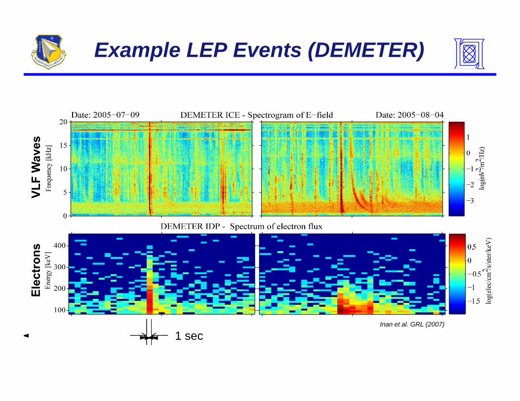
Example LEP Events (DEMETER)W
aves
VLF
ctro
nsEl
ec
Inan et al. GRL (2007)( )
1 sec
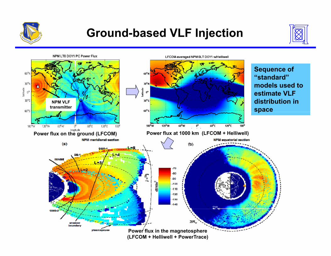
Ground-based VLF Injection
Sequence of “standard”
NPM VLF transmitter
models used to estimate VLF distribution in space
Power flux on the ground (LFCOM) Power flux at 1000 km (LFCOM + Helliwell)
p
Power flux in the magnetosphere(LFCOM + Helliwell + PowerTrace)
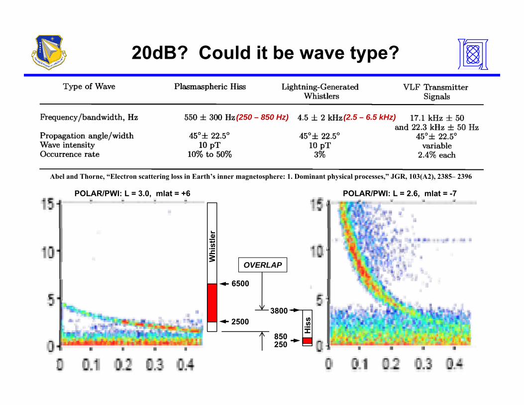
20dB? Could it be wave type?
(250 – 850 Hz) (2.5 – 6.5 kHz)
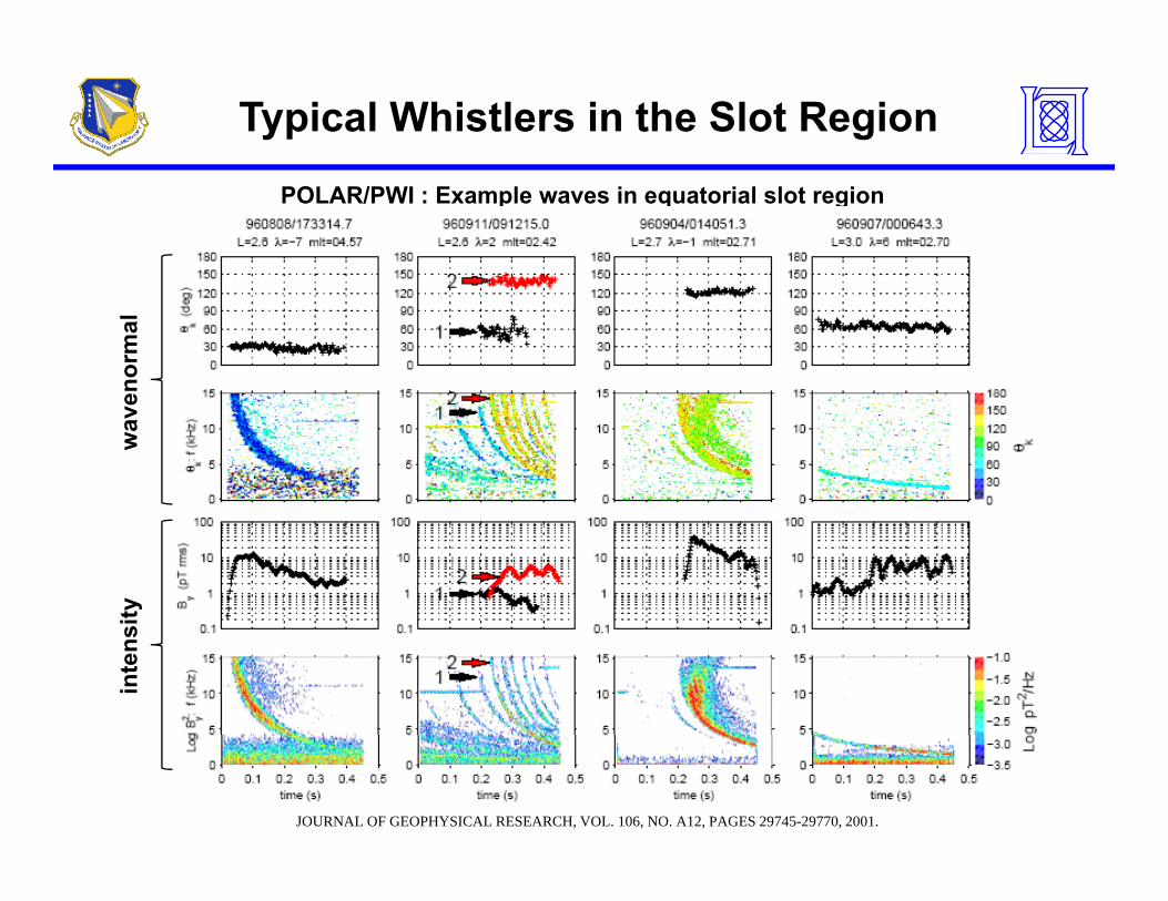
Abel and Thorne “Electron scattering loss in Earth’s inner magnetosphere: 1 Dominant physical processes ” JGR 103(A2) 2385– 2396
POLAR/PWI: L = 2.6, mlat = -7POLAR/PWI: L = 3.0, mlat = +6
Abel and Thorne, Electron scattering loss in Earth s inner magnetosphere: 1. Dominant physical processes, JGR, 103(A2), 2385– 2396
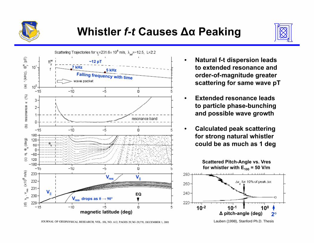
5 kHzorder-of-magnitude greaterscattering for same wave pT
• Extended resonance leads to particle phase-bunchingto particle phase-bunching and possible wave growth
• Calculated peak scatteringfor strong natural whistlerfor strong natural whistlercould be as much as 1 deg
Scattered Pitch-Angle vs. Vresfor whistler with E = 50 V/mfor whistler with E100 = 50 V/m
V||
V||V drops as θ 90°
Vres
EQ
Lauben (1998), Stanford Ph.D. Thesis
10-2 10-1 100
∆ pitch-angle (deg)magnetic latitude (deg)
Vres drops as θ → 90°
2°
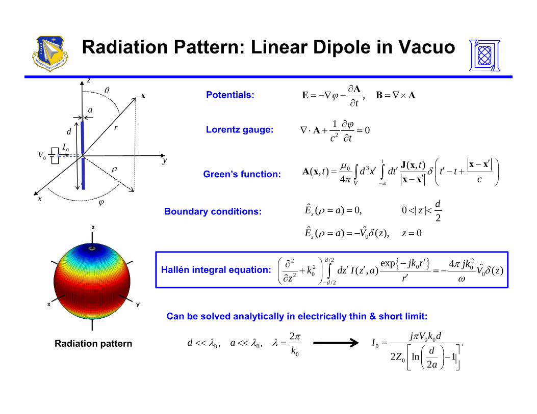
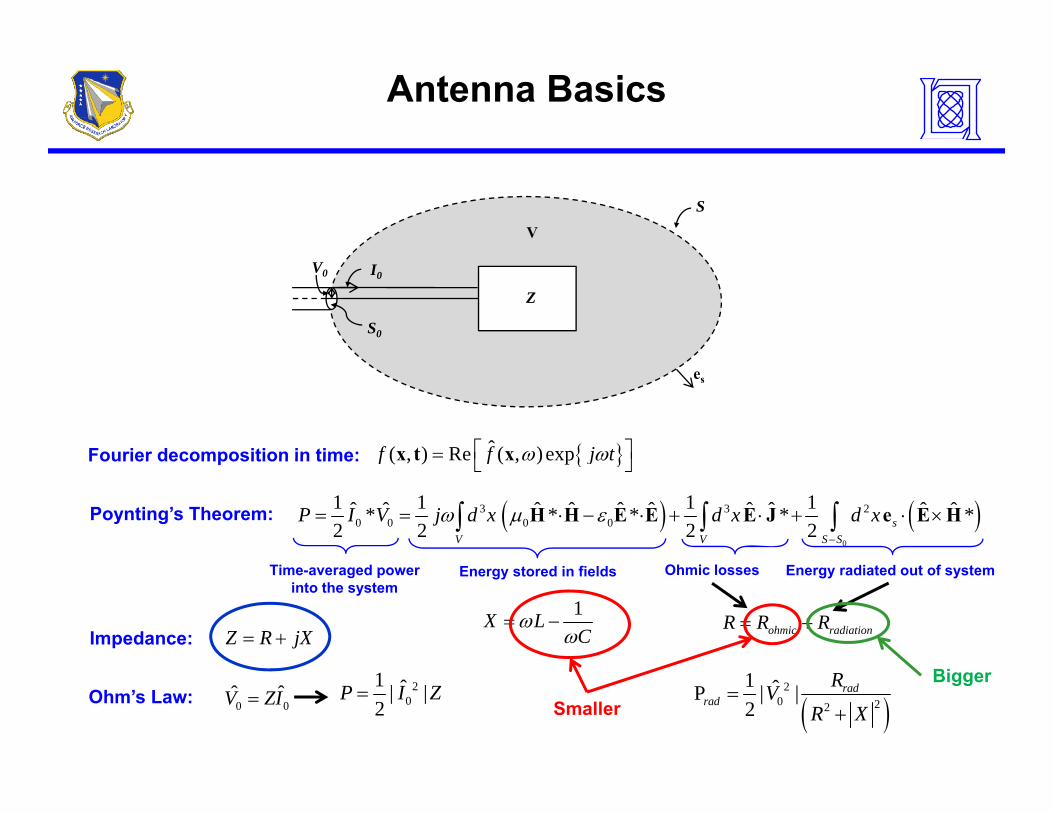
Antenna Basics
S
V
Z
V0 I0
S0
es
ˆ( ) Re ( ) expf f j tω ω⎡ ⎤= ⎣ ⎦x t xFourier decomposition in time: ( , ) Re ( , ) expf f j tω ω⎡ ⎤⎣ ⎦x t x
( ) ( )0
3 3 20 0 0 0
1 1 1 1ˆ ˆ ˆ ˆ ˆ ˆ ˆ ˆ ˆ ˆ* * * * *2 2 2 2 s
V V S S
P I V j d x d x d xω μ ε−
= = ⋅ − ⋅ + ⋅ + ⋅ ×∫ ∫ ∫H H E E E J e E H
Fourier decomposition in time:
Poynting’s Theorem:
ohmic radiationR R R= +1X LC
ωω
= −Z R jX= +
Time-averaged power into the system
Ohmic lossesEnergy stored in fields Energy radiated out of system
Impedance:
0 0ˆ ˆV ZI=
20
1 ˆ| |2
P I Z=Ohm’s Law: Smaller
Bigger
( )2
0 22
1 ˆP | |2
radrad
RVR X
=+
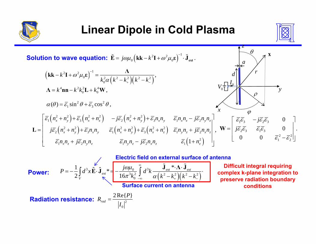
Linear Dipole in Cold Plasmazz
rd
a
θ x( ) 12 20 0 .j kωμ ω μ
−= − + ⋅ extE kk I ε J
( ) 12 2k ω μ−
− + =Λkk I ε
Solution to wave equation:
yρ
d
0V 0I( ) ( )( )0 2 2 2 2 2
0
,kk k k k k
ω μα + −
+− −
kk I ε
4 2 2 40 0 ,k k k k= − +Λ nn L W
2 21 3( ) sin cos ,α θ ε θ ε θ= +
x ϕ1 3( ) ,
( ) ( ) ( )( ) ( ) ( )
( )
2 2 2 2 2 21 3 2 3 1 2
2 2 2 2 2 22 3 1 3 1 2 ,
x y x z x y x y x z y z
x y x y x y x z y z x z
n n n n j n n n n n n j n n
j n n n n n n n n n n j n n
ε ε ε ε ε ε
ε ε ε ε ε ε
⎡ ⎤+ + + − + + −⎢ ⎥⎢ ⎥= + + + + + +⎢ ⎥⎢ ⎥
L1 3 2 3
2 3 1 32 2
00 .
0 0
jjε ε ε εε ε ε ε
ε ε
−⎡ ⎤⎢ ⎥= ⎢ ⎥⎢ ⎥⎣ ⎦
W
( )21 2 1 2 1 1x z y z y z x z zn n j n n n n j n n nε ε ε ε ε⎢ ⎥+ − +⎣ ⎦
1 20 0 ε ε⎢ ⎥−⎣ ⎦
3 3 *1 ˆ ˆ jωμ ∞ ⋅ ⋅∫ ∫
J Λ JElectric field on external surface of antenna
Difficult integral requiring
( )( )3 30
3 2 2 2 2 20
1 ˆ ˆ *2 16
ext extext
V
jP d x d kk k k k k
ωμπ α−∞ + −
= − ⋅ = − ⋅− −∫ ∫
J Λ JE JPower:
Surface current on antenna
g q gcomplex k-plane integration to preserve radiation boundary
conditions2 Re PR =Radiation resistance: 2
0radR
I=Radiation resistance:
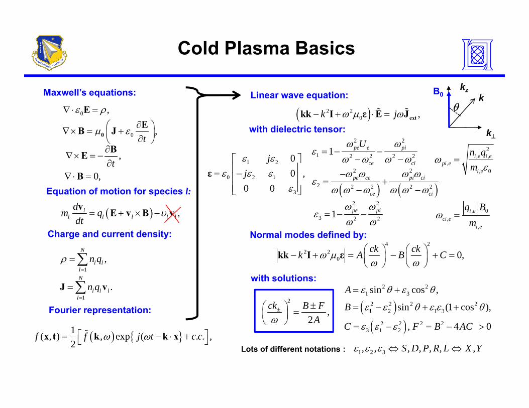
Cold Plasma Basics
0 ,ε ρ∇ ⋅ =E∂⎛ ⎞E
( )2 20 ,k jω μ ω− + ⋅ = extkk I ε E J
Maxwell’s equations: Linear wave equation:
ith di l t i t
B0kz
kθ
0 ,t
μ ε ∂⎛ ⎞∇× = +⎜ ⎟∂⎝ ⎠0
EB J
,t
∂∇× = −
∂BE
0∇⋅ =B1 2
0 2 1
00 ,
jjε ε
ε ε ε⎡ ⎤⎢ ⎥= −⎢ ⎥ε
2 2
1 2 2 2 21 pe e pi
ce ci
Uω ωε
ω ω ω ω= − −
− −2 2pe ce pi ciω ω ω ω−
with dielectric tensor:
2, ,
,, 0
i e i epi e
i e
n qm
ωε
=
k⊥
0,∇ B
( ) ,ll l l l ldm qdt
υ= + × −v E v B v
0 2 1
30 0j
ε⎢ ⎥⎢ ⎥⎣ ⎦ ( ) ( )2 2 2 2 2
pe ce pi ci
ce ci
εω ω ω ω ω ω
= +− −
2 2
3 2 21 pe piω ωε
ω ω= − −
Equation of motion for species l:
, 0,
,
i eci e
i e
q Bm
ω =
1
,N
l ll
n qρ=
=∑N
∑
Charge and current density:4 2
2 20 0,ck ckk A B Cω μ
ω ω⎛ ⎞ ⎛ ⎞− + = − + =⎜ ⎟ ⎜ ⎟⎝ ⎠ ⎝ ⎠
kk I ε
Normal modes defined by:
with solutions:
( ) 1( ) (f f⎡ ⎤
( )( )
2 21 3
2 2 2 21 2 1 3
2 2 2 23 1 2
sin cos ,
sin (1 cos ),
, 4 0
A
B
C F B AC
ε θ ε θ
ε ε θ ε ε θ
ε ε ε
= +
= − + +
= − = − >
2
,2
ck B FAω
± ±⎛ ⎞ =⎜ ⎟⎝ ⎠
1
.l l ll
n q=
= ∑J v
Fourier representation:
t so ut o s
( ) 1( , ) , exp ( . . ,2
f f j t c cω ω⎡ ⎤= − ⋅ +⎣ ⎦x t k k x( )
Lots of different notations : 1 2 3, , , , , , ,S D P R L X Yε ε ε ⇔ ⇔
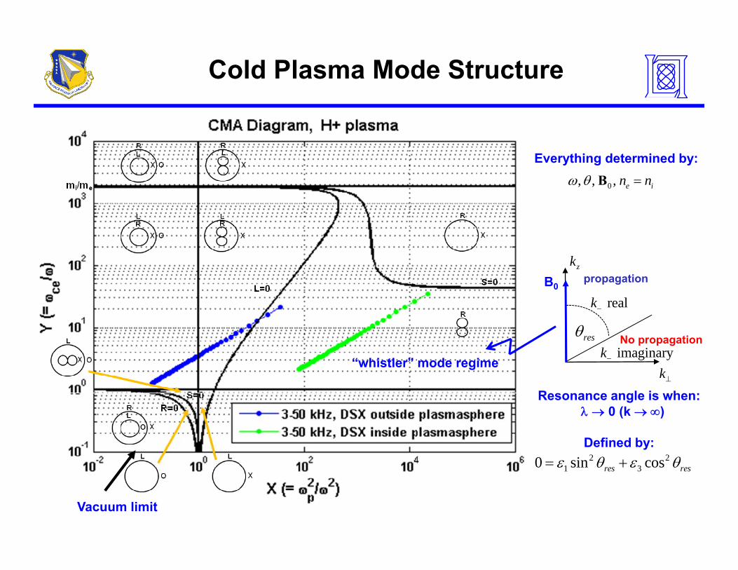
Cold Plasma Mode Structure
θ BEverything determined by:
0, , , e in nω θ =B
real k−
zkB0
propagation
k⊥
resθimaginaryk−No propagation
R l i h
“whistler” mode regime
2 20 sin cosε θ ε θ= +
Resonance angle is when:λ → 0 (k → ∞)
Defined by:
Vacuum limit
1 30 sin cosres resε θ ε θ= +
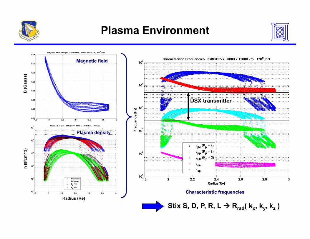
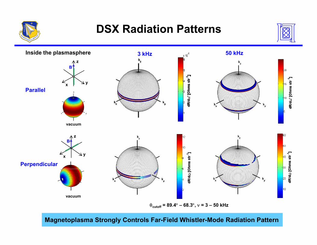
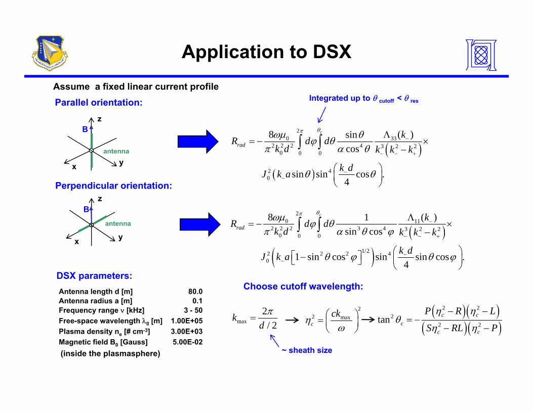
Application to DSX
Parallel orientation:
Bz
Assume a fixed linear current profile
θ
Integrated up to θ cutoff < θ res
B
x yantenna ( )
( )
20 33
2 2 2 4 3 2 20 0 0
2 40
8 ( )sincos
sin sin cos .4
c
radkR d d
k d k k k
k dJ k a
θπωμ θϕ θπ α θ
θ θ
−
− − +
−−
Λ= − ×
−
⎛ ⎞⎜ ⎟⎝ ⎠
∫ ∫
Perpendicular orientation:
Bz
antenna
( )0 4⎜ ⎟⎝ ⎠
( )2
0 112 2 2 3 4 3 2 2
8 ( )1sin cos
c
radkR d d
k d k k k
θπωμ ϕ θπ α θ ϕ
−Λ= − ×∫ ∫
x y ( )
( )0 0 0
1/22 2 2 40
sin cos
1 sin cos sin sin cos .4
k d k k k
k dJ k a
π α θ ϕ
θ ϕ θ ϕ
− − +
−−
−
⎛ ⎞⎡ ⎤− ⎜ ⎟⎣ ⎦ ⎝ ⎠
∫ ∫
DSX parameters:Ch t ff l thAntenna length d [m] 80.0
Antenna radius a [m] 0.1Frequency range ν [kHz] 3 - 50Free-space wavelength λ0 [m] 1.00E+05Plasma density ne [# cm-3] 3.00E+03
max2/ 2
kdπ
=
Choose cutoff wavelength:
( )( )( )( )
2 22
2 2tan c c
cc c
P R L
S RL P
η ηθ
η η
− −= −
− −
22 maxc
ckηω
⎛ ⎞= ⎜ ⎟⎝ ⎠y e [ ]
Magnetic field B0 [Gauss] 5.00E-02( )( )
~ sheath size(inside the plasmasphere)
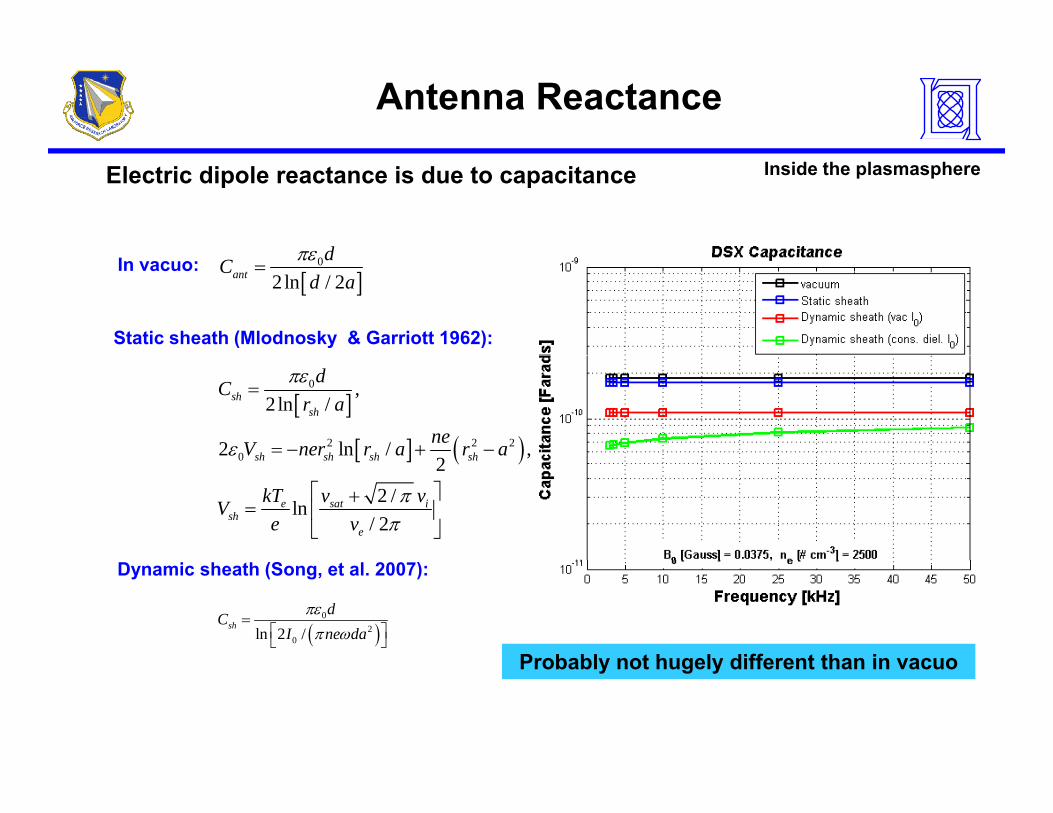
Antenna Reactance
Electric dipole reactance is due to capacitance
dπε
Inside the plasmasphere
In vacuo:
Static sheath (Mlodnosky & Garriott 1962):
[ ]0
2 ln / 2antdC
d aπε
=
[ ]
[ ] ( )
0
2 2 20
,2 ln /
2 ln / ,2
shsh
sh sh sh sh
dCr a
neV ner r a r a
πε
ε
=
= − + −[ ] ( )0 ,2
2 /ln/ 2
sh sh sh sh
e sat ish
e
kT v vVe v
ππ
⎡ ⎤+= ⎢ ⎥
⎣ ⎦
Dynamic sheath (Song, et al. 2007):
( )0
20ln 2 /
shdC
I ne daπεπ ω
=⎡ ⎤⎣ ⎦
Probably not hugely different than in vacuoProbably not hugely different than in vacuo
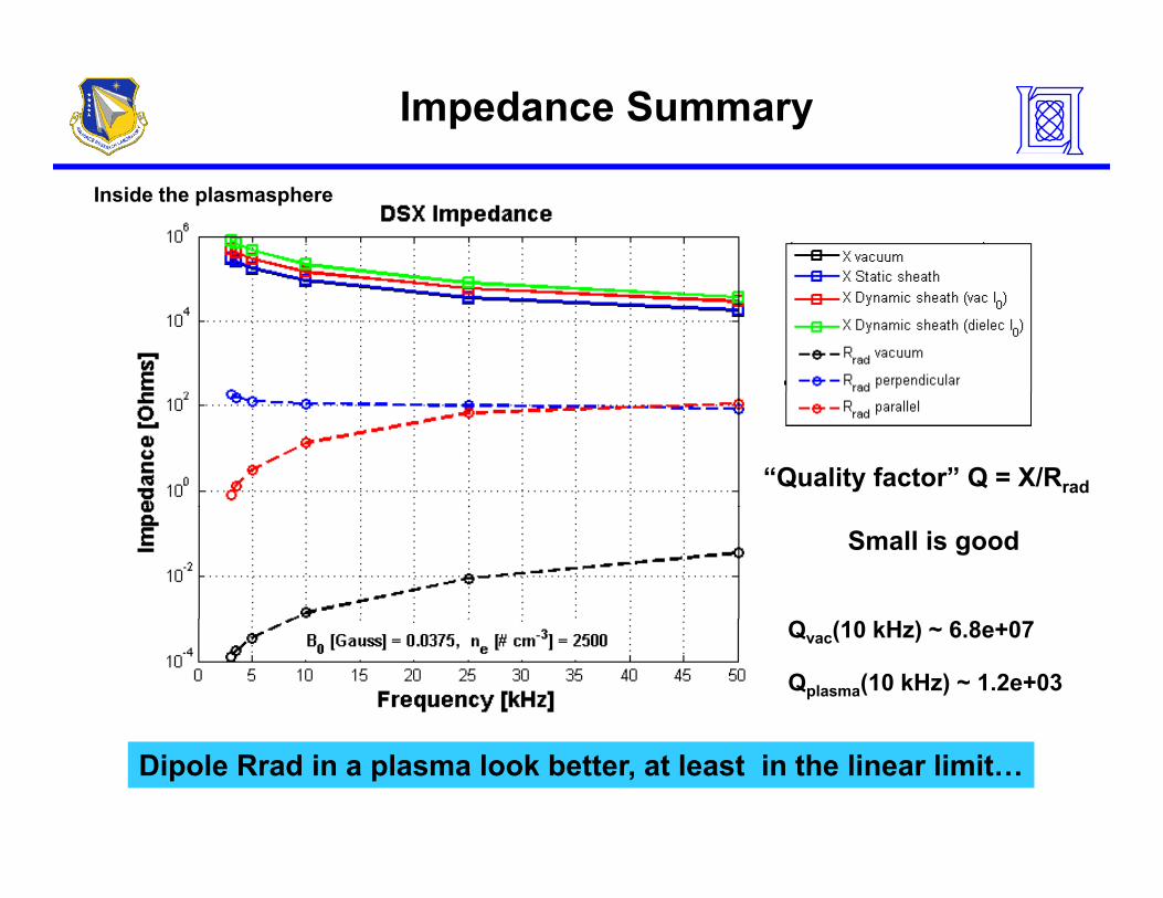
Impedance Summary
Inside the plasmasphere
“Quality factor” Q = X/Rrad
Small is good
Qvac(10 kHz) ~ 6.8e+07
Qplasma(10 kHz) ~ 1.2e+03
Dipole Rrad in a plasma look better, at least in the linear limit…
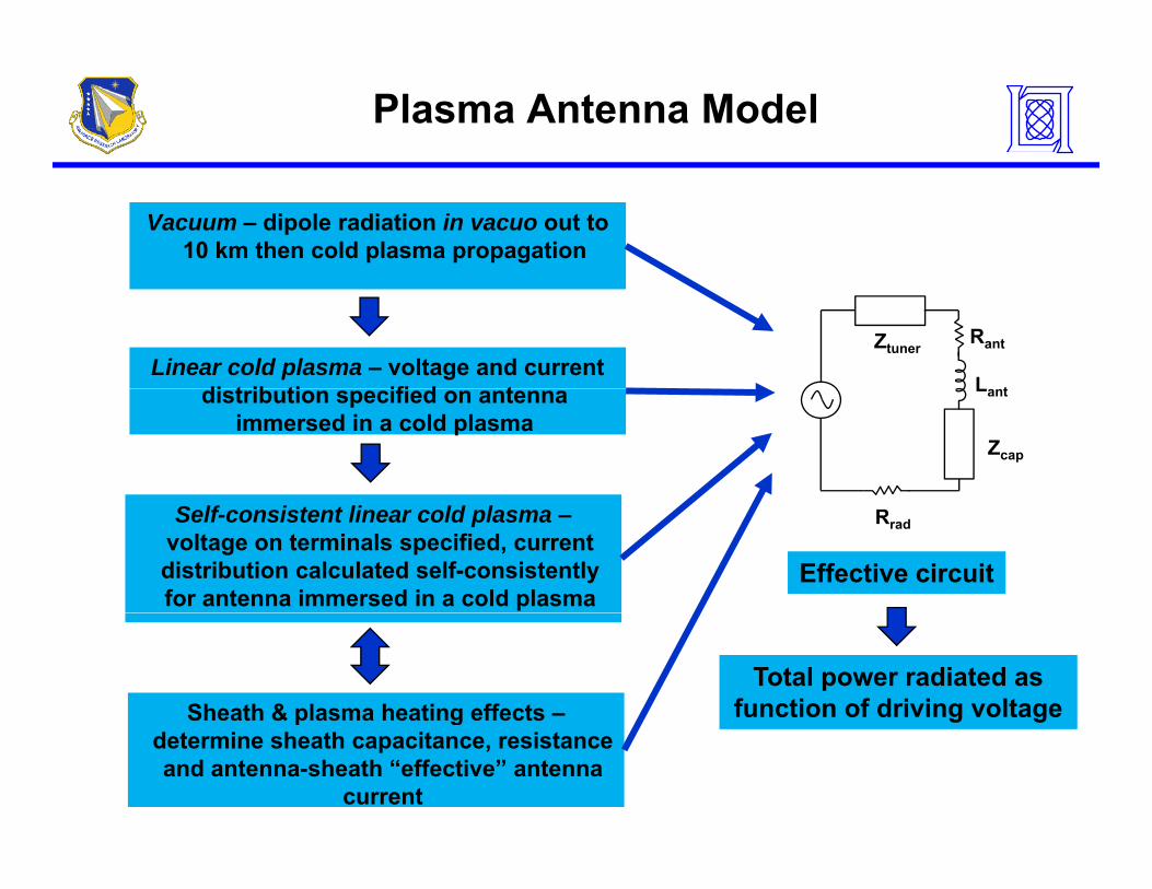
Plasma Antenna Model
Vacuum – dipole radiation in vacuo out to 10 km then cold plasma propagation
Linear cold plasma – voltage and current di t ib ti ifi d t
ZtunerRant
L tdistribution specified on antenna immersed in a cold plasma
Lant
Zcap
Self-consistent linear cold plasma –voltage on terminals specified, current distribution calculated self-consistently for antenna immersed in a cold plasma
Rrad
Effective circuit
Sheath & plasma heating effects –Total power radiated as
function of driving voltage gdetermine sheath capacitance, resistance and antenna-sheath “effective” antenna
current
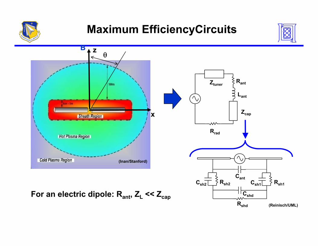
B
Maximum EfficiencyCircuitsB z
θ
ZtunerRant
Lant
x
Rrad
Zcap
(Inan/Stanford)
CantCsh1 Rsh1Csh2 Rsh2
CshdFor an electric dipole: Rant, ZL << Zcap(Reinisch/UML)Rshd