i THE DESIGN AND DEVELOPMENT OF A MOBILE COLONOSCOPY ROBOT by Joseph Christopher Norton Submitted in accordance with the requirements for the degree of Doctor of Philosophy The University of Leeds Institute of Functional Surfaces School of Mechanical Engineering January 2017
Transcript
i
THE DESIGN AND DEVELOPMENT OF A MOBILE COLONOSCOPY
ROBOT
by
Joseph Christopher Norton
Submitted in accordance with the requirements for the degree of
Doctor of Philosophy
The University of Leeds
Institute of Functional Surfaces
School of Mechanical Engineering
January 2017
ii
The candidate confirms that the work submitted is his/her own, except where work which
has formed part of jointly-authored publications has been included. The contribution of the
candidate and the other authors to this work has been explicitly indicated below. The
candidate confirms that appropriate credit has been given within the thesis where reference
has been made to the work of others.
The work included in the papers below is partly used in Chapters 1 – 6:
“RollerBall: a mobile robot for intraluminal locomotion” – IEEE BioRob, 2016 proceedings
Authors: J. Norton, A. Hood, A. Neville, D. Jayne, P. Culmer, A. Alazmani and J. Boyle
I was responsible for the technical work carried-out, the co-authors were responsible for
reviewing the paper.
This copy has been supplied on the understanding that it is copyright material and that no
quotation from the thesis may be published without proper acknowledgement.
CHAPTER 2 LITERATURE REVIEW ........................................................................................... 6
2.1. The colon ....................................................................................................................................... 6
2.2. Colonic inspection and intervention .................................................................................. 8
2.3. Current procedures ................................................................................................................... 8
APPENDIX A: DC MOTOR AND GEARBOX DATA SHEETS............................................. 199
APPENDIX B: 3D PRINTER RESIN (LS600) DATA SHEET ............................................ 201
APPENDIX C: CALCULATIONS FOR THE TISSUE TENSION DURING TRACTION TESTS ............................................................................................................................................ 202
APPENDIX D: AN ALTERNATIVE, SOFT ROBOTIC LOCOMOTION CONCEPT ......... 202
Table 6.1 – The average strain outputs for all Strain gauges and multiple loads. .............. 138
Table 6.2 – The average model coefficients from different masses (SG2). ........................ 139
Table 6.3 – The calibration constants for all strain gauges. ............................................... 140
Table 6.4 – Force sensing validation. .................................................................................. 140
Table 6.5 – The main results from the Manual tests with camera feedback. .................... 166
Table 6.6 – The results from the Manual and Auto force control tests. ............................ 172
Table 6.7 – The results from the manual and automated orientation control tests. ......... 175
Table 6.8 – The results from the manual and automated orientation control tests. ......... 177
Table 7.1 – A summary of how the RollerBall prototype met the desired specifications .. 185
Table A.D.1 – Some methods of achieving variable compliance. ....................................... 206
1
Chapter 1
Introduction
1.1. Background The colon, or large bowel, is part of the gastro-intestinal tract, positioned between the small
intestine and rectum. The thin, sensitive tissue and tortuous shape make this region of the
body extremely challenging to access. This is a significant issue as there are a number of
common diseases that affect the colon: rates of inflammatory bowel disease (mainly
ulcerative colitis and Crohn’s disease) and colorectal cancer are high in the Western world
and are rapidly increasing in developing countries – costing Europe alone billions of Euros
[1, 2]. Colorectal cancer is the world’s 3rd leading cause of cancer related death [3] and as
with all forms of cancer, the stage at which it is diagnosed greatly impacts patient survival
[4, 5]. If detected at any early stage, treatment is relatively simple, cheap and highly
effective. Since the patient will typically have no symptoms and no reason to suspect that
anything is wrong at this point, the only way to ensure early detection is through a reliable
mass-screening program. This should be applied to a subset of the healthy population based
on risk factors, of which age is the most significant. A number of screening methods exist
including fecal occult blood testing, virtual colonoscopy, sigmoidoscopy and conventional
colonoscopy (which is generally considered to be the most common and effective [6]).
A colonoscopy, typically performed under sedation, involves the use of a colonoscope
(Figure 1.1; a long, flexible endoscope) to visually inspect the entire inner surface of the
colon over a period of about 30 minutes.
Figure 1.1 - A conventional colonoscope. [7]
2
Despite their frequent use and powerful diagnostic and therapeutic capabilities,
colonoscopies are a decidedly imperfect solution. The colonoscope is a largely passive device
(only the tip can be actively steered) while the colon is long (up to 1.8m), loosely anchored
and has a highly complex shape with multiple acute bends [8]. The force necessary to
advance the colonoscope can only be applied from outside the patient, so when the tip
encounters resistance (e.g. when trying to navigate a corner) a compressive force is applied
to the flexible shaft, causing it to buckle outwards and even looping back on itself. This can
stretch the connective tissue that anchors the colon to the abdominal wall and cause severe
discomfort. Indeed, more than 10% of attempted colonoscopies are aborted due to
excessive looping and patient discomfort [9]. Unsurprisingly, it can be difficult to convince
asymptomatic people to undergo a painful procedure purely for screening purposes, and
compliance rates – even among those in elevated risk categories – were found to be below
60% [10].
In order to increase success rates and patient compliance with routine colonoscopies, the
procedure should be made as easy, reliable and as comfortable as possible. This in turn will
require new procedure that avoids the shortcomings of the conventional colonoscopy,
including the high forces placed on the colonoscope and the resulting looping. Intuitively,
these phenomena could be eradicated by pulling the instrument from the tip rather than
pushing it from the back and the overall size of the device, and its mobility, improved.
Motivated by this logical hypothesis, an increasing number of research groups have been
working to develop mobile, self-propelled endoscopy robots over the past 20 years. This is
a challenging task and so, despite several attempts, a successful, commercial mobile robot
has yet to be developed.
1.2. The CoDIR project CoDIR (Colonic Disease Investigation by Robot hydro-colonoscopy) is an EU funded project1
that aims to produce a novel robotic alternative to colonoscopy. It is a collaborative effort
by The University of Leeds and The University of Dundee.
The overall aim of the project is to produce a mobile robotic platform to investigate the
colon and carry-out tasks such as taking biopsies – ultimately overcoming the drawbacks of
conventional colonoscopy. The complete system (the device, the console and all the
associated hardware and software) will be developed. The key features of this alternative
approach are to:
1 European Research Council – Reference: CoDIR (268519)
3
Use warm water to distend the colon (hydro-colonoscopy), instead of carbon
dioxide. Preliminary trials have shown that this could reduce patient discomfort and
globally distend the colon. The denser liquid medium could also assist the
locomotion of the robotic device.
Minimize trauma by using a miniature robotic device that applies small forces to the
colonic tissue. This could allow it to be used in weakened colons (such as those with
inflammatory bowel disease) and could further reduce patient discomfort.
Improve mobility within the colon by having full control over the device’s position
and orientation (ie. an on-board locomotion mechanism), increasing diagnostic and
therapeutic efficacy.
If successful, this system would have a global impact. The potential to vastly improve on the
current procedure quality and overall effectiveness is substantial, but so are the challenges.
The work produced over the duration of the project, even if the system itself is commercially
unsuccessful, is likely to further science by introducing novel technologies and insights into
this fast growing area.
1.3. PhD aim and contribution There is undoubtedly significant motivation to research a technology such as this. The area
of mobile in vivo robotics is still relatively new and so any novel technologies and technical
insights developed herein could have an impact on both the medical and robotic fields,
addressing fundamental questions such as “What challenges face the development of
mobile in vivo robots?” and “Could devices such as these be a viable solution to future
medical procedures?”
The aim of this work was to develop a mobile robotic device to traverse the length of a fluid-
filled colon, providing a stable platform for the use of diagnostic and therapeutic tools2. This
included all aspects of development, including: mechanical design, fabrication, electronics
integration and device control. The major steps taken to achieve this included:
1. Reviewing current literature in order to better understand: the unique environment
of the colon; the diseases affecting this region; current methods used to inspect and
intervene in the colon and their limitations; the potential of a mobile robotic
solution, including what has been done previously and what can be learnt going
forward.
2 The robot described in this thesis is one of two robotic devices that will be used in the CoDIR system. One developed at the University of Leeds and the other at the University of Dundee.
4
2. Critiquing an existing concept (RollerBall) that was generated in the CoDIR project
– in light of the reviewed literature – and make necessary design modifications.
3. Completing a detailed design of RollerBall before fabricating a working prototype.
4. Characterising the performance of the individual mechanisms through theoretical
calculations and a series of benchtop experiments.
5. Exploring current methods of gaining traction on the colon and developing a
functional solution by considering literature and a robust empirical assessment of
proposed solutions.
6. Developing the electronics and software required to control the prototype in a
laboratory setting.
7. Assessing the efficacy of the device through a structured set of experiments.
The specific, technical contributions to the medical robotics community are:
A novel method of achieving locomotion in the colon and a detailed assessment of
its efficacy.
Insight into the design and fabrication of small scale prototype, in vivo robotics.
A functional method of gaining traction on the colonic lumen and a suggested
optimal solution.
Work on controlling a mobile robotic device in a synthetic colon environment.
1.4. Thesis structure The individual chapters are summarised below:
Chapter 2 – Literature review
This presents relevant literature, including topics such as current procedures used to inspect
the colon and various locomotion techniques that could be used on a mobile colonoscopy
robot
Chapter 3 – Mechanical design, fabrication and characterisation
This introduces the RollerBall concept – a novel, mobile wheeled device. The design is
described, as well as fabrication and benchtop characterisation of the key mechanical
components.
Chapter 4 – Gaining traction in the colon
A critical requirement for a mobile device that uses the lumen to achieve locomotion is
gaining sufficient traction on the low friction lumen. This explores the challenge in detail and
a suitable tread pattern is proposed after empirically assessing multiple designs.
5
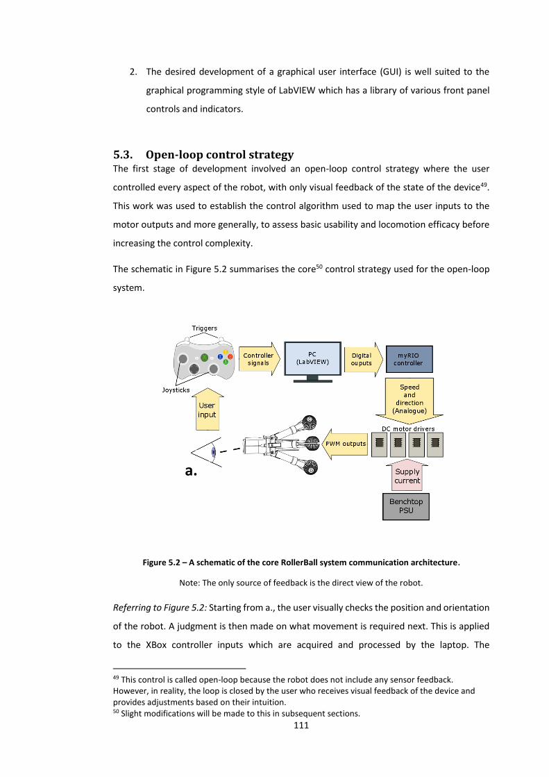
Chapter 5 – System Integration and Open-loop control
This includes work on manually controlling the robot. The associated hardware and software
are developed and a series of tests to assess the efficacy of the control strategy and
locomotion technique are carried-out.
Chapter 6 – Closed-loop control
This chapter builds on the previous, manual control and describes the development of more
advanced, closed-loop control to improve usability, locomotion efficacy and safety.
Chapter 7 – Discussion and Conclusions
Here the key insights into topics such as locomotion efficacy and device usability are
discussed before summarising the work in a series of conclusions.
Chapter 8 – Future work
The final chapter includes suggestions for future developments on the work presented in
this thesis.
Appendix
An appendix provides further detail, including datasheets.
6
Chapter 2
Literature review
This chapter provides an overview of relevant literature on the research of
mobile colonoscopy robots. The topics covered include: the anatomy of the
colon; the need for investigating the colon and the procedures currently
available; the potential of using a mobile colonoscopy robot and; a summary
of various locomotion techniques that could be used. The goal of this chapter
is to communicate the major clinical need for an effective method of directly
accessing the colon and the challenges involved, before concluding what
locomotion techniques are most suited to this unique environment.
2.1. The colon The colon, or large bowel, starts at the ileocecal valve and can thereafter be divided into
several sections (Figure 2.1), starting with the caecum and appendix, followed by the
ascending, transverse and descending colon. The last section is the sigmoid colon (which is
positioned before the rectum and anal canal). The colon is highly variable in its size and
shape, with its length ranging between ca. 1.30 m and 1.88 m in adults [11] [12] (sigmoid
(160 mm) and caecum (40 mm ) [13] [12]). Diameters range from 105 mm in the caecum to
as narrow as 16 mm in other regions of the colon [14] [15]. The shape has a number of
flexures (bends): two are acute (the hepatic and splenic flexures) and, on average, 9.6 are
moderate (< 90o) flexures [11], all contributing to a highly variable, tortuous shape.
The colon is sacculated3 due to the colonic haustra; particularly noticeable when the colon
is distended (insufflated). The colon is partially mobile, attached to the peritoneum4 via
flexible mesocolons5. The lumen is between 0.7 and 1.5 mm thick [16] and is comprised of a
series of distinct, concentric layers, including: the mucosa, muscularis mucosae, submucosa
and muscle layers (Figure 2.1).
3 Comprising of a series of distinct “pouches” or “sacs”. 4 The membrane lining the cavity of the abdomen and covering the abdominal organs. 5 Flat tissue connecting the peritoneum to the colon - blood vessels, nerves and lymphatics branch through this.
7
The tissue’s frictional characteristics have a huge impact on the design and locomotion
efficacy of a mobile robotic device that uses contact based forms of locomotion. As is
discussed in [17], a knowledge of the characteristics are useful to:
Determine the required stroke length to achieve effective locomotion.
Devise an efficient and safe method of clamping to the tissue to manipulate the
friction forces.
Control the device, where knowledge of how these characteristics change with
varying parameters (such as speed and normal load) is useful for the control of the
actuators.
The colon is highly lubricious as it is covered with a layer of shear-thinning mucus. The
resulting frictional characteristics are complex and not well understood – this will be
explored in more detail in Chapter 4.
Figure 2.1 - A diagram of the large intestine (colon), showing its various segments and a cross-section of the multi-layered tissue. [18]
8
2.2. Colonic inspection and intervention There are a number of diseases that can affect the colon, including inflammatory diseases
such as ulcerative colitis and Crohn’s disease, and the more deadly colorectal cancer – the
world’s 3rd leading cause of cancer related death [3]. These require diagnosis and treatment,
with several different procedures available, ranging from completely non-invasive (such as
computed tomography and faecal occult blood testing) to the more invasive and widely used
conventional colonoscopy. These often come at significant economic cost. In Europe alone,
the combined annual direct treatment costs for these are estimated at around €18 billion
[1, 2]. More important than this is the effect these diseases have on quality and length of
life. Worldwide, it is estimated that, annually, over 1 million individuals are diagnosed with
colorectal cancer, with a mortality rate of nearly 33 % [19]. As it is with other forms of cancer,
early diagnosis has a huge impact on mortality: If diagnosed at the latest stage, only 1 in 10
patients will survive longer than 5 years; if diagnosed at the earliest stage, this increases to
9 in 10 [5]. However, the physical properties of the colon and its inherent inaccessibility
make directly inspecting and operating in this environment very challenging indeed. There
are many factors that may lead to late diagnosis but to give an indication of the seriousness,
a study of more than 1 million colonoscopies showed that 29 % of cancers were detected
‘late’ [20].
2.3. Current procedures The is no doubt that having effective diagnostic and therapeutic procedures for the colon is
important; the questions are whether direct access to the colon is required and if so, what
is the best method of achieving that.
2.3.1. Virtual colonoscopy
If direct access to the colon is not required then Computed tomography colonography (CTC)
or virtual colonoscopy may be the best solution to inspect the colon. It is one of the more
modern, alternative techniques used and is specifically focused on colorectal cancer and the
detection of adenomas/polyps. A virtual 3D model of the colon is produced using helical CT
and advanced rendering techniques. It is then meticulously inspected by a specialist for
abnormalities. Bowel preparation and colonic insufflation are both required [21].
This is an attractive procedure with seemingly few drawbacks due to its complete non-
invasiveness. However, the newest, least invasive procedure is not always the most effective
[22]. Table 2.1 presents the main advantages and disadvantages of CTC [21-24].
9
Table 2.1 - The advantages and disadvantages of Virtual colonoscopy (CTC):
Advantages Disadvantages
Non-invasive procedure leads to significantly
fewer complications and improved patient
comfort/adherence.
Insufficient efficacy data. Currently, CTC has a
lower sensitivity (ability to detect polyps),
particularly with small polyps (< 6mm)6 [21].
With polyp sizes < 6 mm, 6 – 9 mm and > 9 mm
the sensitivity of CTC is estimated as 29%, 66%
and 97% respectively. In comparison, the
estimated sensitivity for CC is 80%, 88% and
91% respectively [23].
Bowel preparation often less intensive and
sedation not required.
Poor detection of flat adenomas and general
lack of histology information.
Effective at viewing entire colon, even in cases
where there is severe narrowing of the colon.
Long term effects of radiation unknown,
although one study estimates that there is still
a risk (0.14%) of cancer post CTC [21].
Can detect extra-luminal abnormalities. 7-16% of patients who undergo CTC a
conventional colonoscopy anyway [21, 23].
Requires more frequent follow-ups.
Is less cost effective in most cases.
Can be time consuming due to the required
collection and manipulation of data.
Although presenting some attractive advantages, two significant limitations of CTC, when
compared to procedures that directly inspect/access the colon, are its inability to carry out
therapeutic and robust diagnostic tasks such as polypectomies and biopsies (this is crucial
for the treatment of colorectal cancer) [25] and its poor performance at detecting small or
flat abnormalities (which would most likely be the case with early stage cancer). CTC is
merely a diagnostic tool aimed at the detection of polyps and can augment but not replace
the all-round, complete diagnostic and therapeutic procedure of something like the
conventional colonoscopy.
It would appear that direct access (using a colonoscope, for example) is required the
majority of the time. Some of the more common indications are listed in Table 2.2 [26].
6 The polyp size threshold determining whether or not a polypectomy is necessary is currently a controversial issue. Most experts recommend the threshold to be > 6 mm due to the prevalence of cancer in patients with diminutive adenomas being approximately 0.1%.
10
Table 2.2 - Colonoscopy indications [13]:
Colonoscopy indications
Evaluating an abnormality found using barium enema.
Evaluation of unexplained gastrointestinal bleeding.
Unexplained iron-deficiency anaemia.
Investigating the colon for synchronous cancer or neoplastic polyps.
Precise diagnosis of chronic inflammatory bowel disease.
Unexplained, clinically significant diarrhoea.
Diagnosis and treatment of colonic lesions.
Foreign body removal.
Excision of colonic polyp.
Decompression of acute nontoxic megacolon or sigmoid volvulus.
Balloon dilation of stenotic lesions.
Palliative treatment of bleeding neoplasms.
Marking neoplasms for localization.
It is easy to see why there are estimated to be more than 14 million colonoscopies carried
out around the world each year [27]. Due to the nature of the procedure, there remain
several contraindications to performing a conventional colonoscopy, the primary one being
severe inflammatory bowel disease. In these cases, the colonic wall is particularly sensitive
to perforation [13] and alternative procedures are required.
2.3.2. Conventional colonoscopy
By far the most common invasive procedure for inspecting the colon is the conventional
colonoscopy; this is the benchmark that any alternative should improve on. The total
colonoscopy is a procedure by which the entire colon can be inspected and, in some cases,
allows for local therapeutic action. It was first described by Shinya and Wolff in 1969,
bringing about the development of an effective means of diagnosing diseases and carrying-
out small procedures, such as polypectomy7, in situ. Since then the colonoscopic procedure,
and the equipment used, have improved significantly, resulting in it becoming the “gold
standard” for the detection and prevention of colorectal neoplasms, as well as the diagnosis
of a number of colorectal diseases [13].
7 Removal of an abnormal feature called a polyp.
11
2.3.2.1. Colonoscopy equipment
The conventional colonoscope is a flexible tube, 130-170 cm long and 1.3 - 1.5 cm in
diameter. It is fitted with an actuated section at the distal end to facilitate passage around
the tortuous colon. This can be bent in any direction using the steering controls. The core of
the colonoscope usually contains a channel for tools and cables for the various lights and
cameras present at the tip of the instrument (Figure 2.2). Additional equipment is required
to carry out a colonoscopy, including a display for the real-time images from the colonoscope
and a unit to regulate pressure within the colon.
Figure 2.2 - Colonoscope within the colon, including detail of the colonoscope tip. [28]
2.3.2.2. Outline of the current procedure
When required, a total colonoscopy procedure consists of four discrete phases: bowel
preparation, sedation, colonoscope insertion and colonoscope withdrawal [13]. These are
briefly described below:
12
Bowel preparation
Bowel preparation is an unpleasant but essential part of the colonoscopy, required to
improve vision of the colonic mucosa. Most preparation methods involve the administration
of an oral laxative the day before the colonoscopy in order to purge the colon of any residual
matter. The intake of clear fluids during this period is highly encouraged to prevent
dehydration. Most procedures involve the ingestion of PEG-ELS (a balanced electrolytic
solution containing polyethylene glycol) or Phosphosoda (sodium phosphate). A strict
dietary regime is then followed, with regular ingestion of the selected laxative and
electrolyte solution. Antispasmodics are usually administered during the procedure as
circular muscle spasticity is known to impair vision of the colon.
Sedation
Most colonoscopy procedures can be performed successfully without sedation but,
endoscopists are encouraged to have a flexible attitude towards patient sedation. This is
because of the anxiety understandably involved in the diagnosis of diseases, embarrassment
due to the invasiveness of the procedure and pre-empted pain.
Colonoscope insertion
It is common for colonoscopists to perform a total colonoscopy hundreds of times and yet it
remains a difficult technique to perfect. It is said that an average of 275 procedures are
required before achieving competence [29]. The procedure is difficult because it involves
the manual insertion of a flexible tube into a compliant, sensitive, tortuous-shaped and
mobile colon using an external force. The exact technique used varies but what is clear is
that the procedure requires significant expertise, “feel” and dexterous manipulation of the
colonoscope.
In brief, a colonoscopy involves the insertion of a colonoscope into the anus with the aim of
reaching the caecum and thus observing the whole colon. This requires the simultaneous
controlling of the steering wheel controls with one hand and manual insertion of the
colonoscope shaft with the other (Figure 2.3). The colonoscope advances when a
combination of external force and internal tip steering is used. The external application of
pressure8, and combined insertion and withdrawal movements, are used to control the
buckling of the device and prevent undesirable loops forming. These loops often prevent
completion of the procedure, can increase patient discomfort and can even result in
perforation of the colonic wall (Figure 2.4). To aid in the advancement of the colonoscope
8 To the abdomen via the surgeon’s hand.
13
and visualisation of the tissue, the colon is distended using a pressurized gas (usually air or
carbon dioxide). This distension often causes patient discomfort but performs an essential
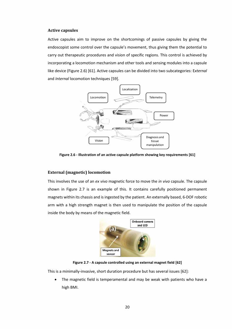
and electronics that exceed the limits of current technology. A more plausible approach is
to not restrict the size and shape to a capsule. The resulting devices could simply be called
“Mobile colonoscopy robots”.
2.4. A mobile colonoscopy robot The development of a fully mobile, semi-autonomous diagnostic and therapeutic robotic
platform could be a vast improvement on conventional colonoscopy. The use of a warm fluid
(hydro-colonoscopy) could further improve colonic investigation by increasing caecal
intubation rates and by reducing patient discomfort. The focus of the CoDIR project is to use
a combination of these two methods to realise an optimum solution to colonic inspection
11 In addition to this, the capsule will always be pressed against the side of the lumen nearest the external magnet, further reducing the efficacy of on-board tools.
22
and intervention. Below is a list of the general requirements of such a robotic device for use
in a hydro-colonoscopy environment.
2.4.1. Device requirements and environmental challenges
The mobile robotic platform will be required to traverse a very unique and challenging
environment. This is particularly true in the case of hydro-colonoscopies, where the device
will not only be operating in a sensitive, compliant, tubular environment with varying shapes
and sizes, but will also be fully submerged in a liquid. The device may use the surrounding
tissue to push against or anchor itself. This will introduce new challenges considering the
anatomy: the tissue is sensitive to perforation, extremely compliant, irregularly-shaped and
has a low coefficient of friction due to a thick layer of mucus – the lumen giving rise to a
complex set of frictional characteristics. Alternatively, the device could swim through the
liquid medium with little to no contact with the surrounding tissue (provided there is
sufficient colonic distension). A device operating in such an environment would have a
number of requirements for it to be successful. The more important requirements with the
reasons for each, are shown in Table 2.5 and continued in Table 2.6:
Table 2.5 - General requirements for a mobile robotic platform for hydro-colonoscopy.
Requirement Description Justification
Small size Have a rigid diameter ideally less than 26 mm and a length less than 40 mm [8, 14, 15, 63].
Studies on the anatomy of the colon estimate a minimum colon diameter of 26 mm, giving an indication of the maximum width/diameter of a rigid robot. A short length would improve mobility around acute flexures.
High speed
Complete a standard colonoscopy in a one hour timeframe, preferably reaching the caecum in 6 – 8 min [63].
In order to be a viable replacement for a conventional colonscope, a MCR should not lengthen the already time consuming procedure as this could increase procedural complications and costs.
High mobility
Traverse the full length of the large intestine; turning corners, stopping, starting and reversing its direction at the caecum [63].
Mobility is crucial in this case as it would directly affect the diagnostic performance of the device. The mobility is also crucial in ensuring successful caecal intubation.
Safe Cause little to no damage to the surrounding colonic tissue [63].
The colonic tissue is sensitive, particularly in patients suffering from diseases such as diverticulosis. The interaction of the device with the colon, in terms of material chemistry and physical contact, must not cause damage to the tissue. As with all other in vivo medical devices, this is of paramount importance to this device.
23
Table 2.6 - General requirements for a mobile robotic platform for hydro-colonoscopy (Continued).
Requirement Description Justification
Be adaptable Operate in a wide variety of patients.
In order to be successful, the device should be able to operate in patients with a large variability in colon diameter, shape and tissue surface features.
Provide a stable platform
Provide a stable platform for the use of cameras and biopsy tools.
In order to successfully view details of the colon with an on-board camera, a stable platform is required with a smooth locomotion technique. Additional therapeutic tools require a stable, anchored device in order to operate accurately and efficiently.
An effective locomotion technique
Have a robust locomotion mechanism and appropriate locomotion technique [63].
Locomotion is potentially the greatest challenge involved in designing such a device. The technique used should be appropriate to the unique environment of the colon; it must provide efficient and reliable locomotion in vivo (despite the tissue frictional characteristics and mechanical properties). The locomotion technique will determine the procedure length and overall effectiveness of the device [63].
Be robust Overall robust device and if possible, an included failsafe.
Failure in vivo would have serious implications. A failsafe may have to be included to manage the potential risks of device malfunction.
Overcome tether drag (thrust)
The device should have the ability to pull a tether behind itself, achieving an average thrust of at least 1 N12 to overcome the associated drag.
Ideally, an in vivo device should be wireless as it would increase biocompatibility and device mobility. However, most devices include a tether as it simplifies on-board electronics, power supply and provides a means of manually removing the device in the event of a malfunction (failsafe).
Easy to use The device should operate in the colon with minimal input from the user.
A significant cause of many of the drawbacks of colonoscopy is the difficulty of the procedure (and the required experience) [36] [38]. A procedure that is easy to perform will allow more attention to be given to important tasks such as diagnosis and surgical intervention.
These major requirements will be used to assess the effectiveness of current devices and
the design of future concepts.
12 This is an estimate from preliminary experiments conducted by researcher in the CoDIR group.
24
2.5. Locomotion techniques It is clear that choosing an appropriate form of locomotion is crucial for the effectiveness of
the device. It must take into account the unique geometry of the environment, as well as
the tissue and lumen properties. Although there has been significant research focus on the
design of active devices to traverse the intestine – using a number of different forms of
locomotion – no device has fully succeeded due to the challenging environment.
Furthermore, substantial work has been done on devices operating in a collapsed colon and
less on devices designed to operate in a distended colon13. The tissue properties and colonic
environment vary considerably between a collapsed and distended colon, therefore the
design features will vary considerably too.
There are two broad classes of locomotion technique that could be used: Contact-based
locomotion and Swimming in the liquid filled colon (having limited to no contact with the
tissue). This section includes a number of designs that have been (or could be) used for an
active, mobile colon-based device. The focus of this thesis is to design a device for use in a
hydro-colonoscopy procedure and so the effectiveness of each design for use in this specific
environment will be reviewed in the following format: Description of the technique; an
example device and; whether it is feasible (when considering this context).
2.5.1. Swimming forms of locomotion
The use of a liquid to distend the colon during hydro-colonoscopy is a relatively new
technique that has yet to be widely adopted. Consequently, no robotic devices purposefully
built for swimming in the tortuous, fluid-distended colon currently exist. One of the primary
advantages of hydro-colonoscopy is the reduced patient discomfort. Intuitively, if a device
could be designed to swim within the colon with limited to no contact with the tissue then
discomfort could be further reduced, as would other complications such as tissue damage.
As there are currently no hydro-colonoscopy specific robots, general swimming techniques
that are used, particularly in small robotic devices, will be investigated.
2.5.1.1. Conventional propeller
Description: Using conventional propellers to provide propulsion.
Example: Carta et al. [64] developed a propeller-based capsular device for use in the fluid
filled stomach. The neutrally buoyant prototype capsule (15 x 40 mm), shown in Figure 2.8,
13 Additionally, no recorded work has been found on devices designed to operate in a fluid-distended colon (hydro-colonoscopy).
25
comprises of four propellers (3 mm diameter), each powered by a DC motor (4 x 8 mm, Didel
MK04S-24).
Figure 2.8 - A device powered by four conventional propellers. [64]
Feasibility: Tests showed “satisfactory results in terms of controllability” but “limited
autonomy” with the operator controlling the device manually with a joystick [64]. Although
this capsule originally had a different application, such a design could be used in a hydro-
colonoscopy procedure. The small size and its controllability mean that it has great potential
to traverse the tortuous fluid filled colon. However, limitations such as low thrust (likely
preventing the use of a tether) and the restricted space for on-board tools suggest that it is
not suitable for this specific application.
2.5.1.2. Ring thruster
Description: Replacing conventional propellers with ring propellers as a form of propulsion.
Example: Kennedy et al. [65] describe the design of a ring propeller, shown in Figure 2.9. This
differs from a conventional propeller in that there is no central hub connecting the blades
to the drive shaft. Instead, the blades are connected to an outer ring which is the rotor of an
electric motor. A stator ring around rotor completes the propeller unit.
Figure 2.9 - An exploded view of a ring propeller. [65]
26
Feasibility: It was seen that these propellers were between 40 and 80% more efficient than
alternative, conventional propellers. Other advantages of ring propellers include [66]:
Compact mechanism due to the exclusion of gearing and drive shafts.
Housing of the blades within the motor unit improves the safety aspect.
The design allows for close proximity, counter rotating propellers.
Little work has been done on miniature versions of this type of propulsion. The manufacture
would undoubtedly be challenging but, if an efficient motor can be manufactured and the
thrust is scalable from the larger ring propellers previously tested, this offers a promising
solution to propelling a colon-based capsule.
2.5.1.3. Rotating helix
Description: Rotating a helix will provide thrust as the thread-like structure pushes against
the viscous fluid medium.
Example: Chen et al. [67] designed the device shown in Figure 2.10. It is designed for use in
an endovascular environment and so must be very small (ideally < 3 mm). It has four rotating
helixes to propel and steer the device.
Figure 2.10 - Example of a device that uses rotating helixes. [67]
Feasibility: These devices can be significantly miniaturized and use flexible tails/helixes and
so could provide an attractive, biocompatible solution to swimming within small, in vivo
environments. Such devices do, however, have significant disadvantages, including: the
predicted thrust force is very low and the propulsion is more effective in a viscous medium,
not the watery medium present in hydro-colonoscopy. A device with a helix diameter of 5
mm has a thrust of approximately 6 mN at 200 rad/s [68], much too low for a tethered
device.
27
2.5.1.4. Pressurized jet
Description: Using a simple, high pressure jet of water to produce thrust (from the inertial
forces of the accelerated water).
Example: Mosse et al. [63] developed the device shown in Figure 2.11. This was more of an
internally propelled colonoscope than a fully mobile capsule device, although the propulsion
method could be used for a capsule device if a tether is included. Mazumdar et al. [69]
designed and built the compact, highly manoeuvrable device shown in Figure 2.12. The robot
steers itself by means of on-board centrifugal pumps. Although these are used for steering,
they could also be used as a form of primary propulsion in a similar device such as that stated
in [70], which has four eccentric rotor pump units based on the Downingtown-Huber design.
Figure 2.11 - An example of a device that uses a pressurized jet. [63]
Figure 2.12 - A device that uses on-board centrifugal pumps. [69]
Feasibility: An attractive feature of using pressurized water jets for propulsion is that, like
conventional propellers, they can be easily controlled in terms of direction and speed by
using electronic valves. This in turn makes devices controlled by them highly mobile [69].
There is also an absence of external rotating parts, such as propellers, which is expected to
improve the safety aspect. However, the difficulty of achieving sufficient thrust arises when
such devices are scaled-down for use in vivo because of their inefficiency (50% [70]). The
well-known fact remains that jet-propulsion is more suited to low speed applications, and
propellers to high speed applications. Additionally, on-board pumps attain a relatively low
28
thrust for their size, with the 25 mm diameter pumps in [69] only achieving 0.125 N. An
alternative is using a tether to transmit the pressurized fluid from an external pump to the
device, as in [63]. This has the disadvantage of high drag from the tether (especially in the
tortuous colon)14. Furthermore, the tether would have to be up to 2 m long whilst being as
thin as possible. Having sufficient flow through such a tube would require a very high
pressure. The device in [63] used 20 Bar and only managed to move a distance of 300 mm
proximal to the anus before resistive forces became too large. Some minor tissue damage
was seen and would be expected to worsen if the jet pressure was increased to the required
amount.
2.5.1.5. Vortex rings
Description: Loosely inspired by the propulsion of squid and jelly fish, this involves the
generation of traveling vortex rings using pulsed jets of water through a narrow orifice.
Example: This form of propulsion was investigated by Mohseni et al. [71], as well as a
number of other authors. It is said that this form of pulsed jet is more efficient than a steady
jet of equivalent mass flow rate, and so aims to improve on the previously mentioned
pressurized-jet designs. A simple piston pump is used to firstly draw in water and then
rapidly eject the water through the same orifice. As the stream of water travels out the
orifice it wraps-up into a traveling vortex ring. This procedure is repeated in short succession
to achieve a row of vortex rings and a positive net thrust (Figure 2.13).
Figure 2.13 - The generating of vortex rings. [71]
Feasibility: This form of locomotion improves on the pressurized-jet’s low efficiency, whilst
maintaining the same advantages of control and biocompatibility. However, insufficient
work has been carried on scaled-down versions of this propulsion method and as such, the
achievable thrust is still relatively low compared to the propeller alternatives. In [72], a 25
mm piston, actuated using a voice-coil, produced a maximum thrust of approximately 70
mN. This value was expected to rise to approximately 250 mN if an improved voice-coil
14 A conventional tether containing thin electrical wires would likely have a smaller diameter and, potentially, lower stiffness (improved flexibility).
29
actuator was used. Therefore, significant work would need to be carried out in order to
achieve the desired 1 N from a pump with a diameter less than 25 mm.
2.5.1.6. Fins (fish-like)
Description: Simple fish-like locomotion involving side-to-side movement of a fin. Some use
a propulsive wave travelling down the length of the body and/or fin to provide a net forward
thrust.
Example: Guo et al. [73] developed the device shown in Figure 2.14. It is designed to mimic
the undulating swimming style of fish, where a propulsive wave is propagated down the
body and/or fin. Ionic exchange Polymer Metal Composites (IPMC) actuators were used to
achieve the motion. Wang et al. [74] developed a similar device, except Shape Memory
Alloys (SMA) were used with an elastic energy storage mechanism to improve actuation
efficiency (Figure 2.15). Takagi et al. [75] designed a robot to mimic the swimming style of
rays (Rajiform swimming). They achieved this using multiple IPMC actuators positioned
parallel to each other down the length of the fin (Figure 2.16). Actuating them sequentially
produced a traveling wave which then resulted in a propulsive force. Kosa et al. [76]
designed a swimming device that propels itself by means of a travelling wave, produced
using piezo-electric micro-actuators (Figure 2.17).
Figure 2.14 – Example #1 of a simple finned device using IPMC actuators. [73]
Figure 2.15 - Example #2 of a simple finned device using SMA actuation. [74]
30
Figure 2.16 - Rajiform swimming using a flexible fin. [75]
Figure 2.17 - Example #3 of a simple finned device. [76]
Feasibility: Fish-like propulsion is said to more efficient than propeller based propulsion, with
the added advantage of a smaller turning radius [74] (a clear benefit for a device operating
in the tortuous colon). The propulsion mechanism could be made to be simple and compact,
potentially allowing these devices to be significantly miniaturized. Furthermore, the flexible
nature of the devices means they would increase their feasibility for use in sensitive,
constricted areas. However, swimming using a fish-like form of locomotion also has its
drawbacks, the most notable is that, while recorded velocities were high (up to 112 mm/s
in [74]), the propulsive forces of such devices are very low (3.75 x 10⁻⁴ N [73]). This severely
restricts the possibility of tethered devices as they would most likely have insufficient thrust
to overcome the associated drag. In hydro-colonoscopies there may be air pockets and/or
stenosis of the colon and a swimming device would struggle in these cases, reducing its
overall feasibility for practical use.
31
2.5.1.7. Summary – swimming forms of locomotion
Swimming devices designed for use in the colon would have a clear biocompatibility
advantage as they would have limited contact with the sensitive colonic walls. This lack of
lumen contact and potential for miniaturisation could result in high mobility and thus caecal
intubation rates could be high. However, two critical issues currently remain with this form
of locomotion:
1. Generating sufficient thrust – This seems to rule out fin-based methods as well as
most pressurized jet methods, although pulsed vortex rings and propellers (both
conventional and ring) seem more promising. The most capable methods could still
struggle to achieve sufficient thrust to pull a tether.
2. Carrying supplementary tools – By their very nature, these devices are designed to
be small, compact and do not include a means of anchoring themselves against the
tissue for stability. This complicates the inclusion of on-board tools as they not only
add weight and complexity but are more effective from a stable (fixed) platform.
These limitations point towards the use of the surrounding tissue for propulsion and
stabilisation (anchoring).
2.5.2. Contact-based forms of locomotion
The two major issues present in swimming forms of locomotion could be solved by using the
surrounding colonic walls as an anchor to push or pull against in order to propel the device.
It would also provide a means of keeping the device stationary, allowing supplementary
tools to be used. Relying on the tissue to propel the device does present some new
challenges, including:
Maintaining a high level of mobility whilst being in continuous contact with the
tissue.
Attaining sufficient traction and having a large enough stroke15 to carry out efficient
motion in the flexible, low friction environment.
Adjusting to the variable shape and size of the colon while achieving the above.
Realizing all the aforementioned without damaging the sensitive colonic tissue.
15 Because of the inherent low friction there is likely to be a degree of slip during contact. When traction is made, the soft, elastic tissue needs to be deformed a certain degree before providing sufficient resistance for locomotion.
32
Below are some locomotion techniques currently used for colon-based devices, and others
from different applications that could be adapted for use in this context:
2.5.2.1. Impact-driven
Description: This maintains the compact shape of a capsule and locomotion is achieved using
the inertia of a moving mass to propel the robot forwards (Figure 2.18). This can be described
as “vibratory locomotion” [77].
Example: The device designed by Carta et al. [77] uses an off-centre rotating mass to achieve
vibratory locomotion. Because the mass is off-centre, a net forward force is produced and
the capsule advances in small steps.
Figure 2.18 - Impact-driven capsule device. [77]
Feasibility: This form of locomotion is most effective on hard surfaces and so would be
extremely inefficient in the mobile and compliant colon [77] – the energy from the vibrating
mass would be dissipated through deforming the visco-elastic tissue. Furthermore, although
the capsule is compact, the lack of fine movement control, lack of device steering and
anchoring mechanism would not allow the housing and effective use of supplementary
tools.
2.5.2.2. Elongated toroid
Description: This is a unique form of locomotion designed to mimic the cytoplasmic
streaming ectoplasmic tube found in amoebae Figure 2.19, a.
Example: Hong et al. [78] designed the “whole-skin locomotion device” shown in Figure 2.19,
b. It aimed to mimic the natural system by contracting one end of a mobile toroid. This
results in the extending of the opposite end of the device as the toroid turns itself inside-out
33
(Figure 2.19, a.). Activating the appropriate ring actuator (eg. 1a, 2a or 3a in Figure 2.19, a.)
as it reaches the end of the toroid results in a continuous forward motion.
Figure 2.19 - Elongated toroid form of locomotion. a. The locomotion technique. b. An example of such a device. [78]
Feasibility: This has the potential to effectively move inside the colon as the whole body
generates traction whilst the front advances16. It has the additional advantages of reduced
tissue damage and having a compact shape which could result in high caecal intubation
rates. However, this is a complex locomotion mechanism that has not yet been fully
developed or tested in vivo. Furthermore, the lack of fine steering control and the fact that
the actuation mechanism dominates the composition of the body reduces its ability to house
16 This could also exploit the larger magnitude static friction.
a.
b.
34
additional tools and cameras. It also does not have a means of actively changing its diameter
which may limit its use in a distended colon (due to less device-tissue contact).
2.5.2.3. Wheeled/tracked
Description: This involves the use of conventional wheels or tracks, spaced evenly around
the body, to propel the device through a tubular environment. Some form of extension
mechanism is often used to ensure the wheels/tracks remain in contact with the surface as
the diameter of the tubular environment changes.
Example: Sliker et al. [79] developed the tracked device shown in Figure 2.20, a. This device
has a track on each side to provide propulsion, with a textured track surface to improve
traction. It was designed for use in the small bowel, but is not constrained to it. During one
study, it was tested and deemed suitable for natural orifice transluminal endoscopic surgery
(NOTES) and for use in the colon.
Kwon et al. [80] designed and built the pipeline inspection robot shown in Figure 2.20, b.
Although not designed for use in vivo, such a design could be implemented due to its ability
to adapt to varying diameters (advantageous for maintaining traction within the colon). A
similar device was developed by Park et al. [81]. This comprises of a single module which has
the ability to adapt more easily to changing diameters and has improved mobility around
bends (Figure 2.20, c.). Liu et al. [82] used wheels instead of tracks, with a flexible, modular
layout to improve mobility around bends (Figure 2.20, d.).
Lambrecht et al. [83] show how an alternative to both wheels and tracks, Wegs™, could be
used to improve mobility over uneven terrain (Figure 2.20, e.).
35
Figure 2.20 - Various wheeled / tracked devices. a. – c. Tracked devices. [79], [80], [81] d. Pipe inspection, wheeled device. [82] e. Device using Whegs. [83]
No such device has currently been designed to replace a colonoscope and to be used in a
distended colon, particularly one that is fluid filled. Therefore, some general assumptions
will have to be made on the feasibility of such devices.
Feasibility: In one study, the robot described in [79] was successful in achieving locomotion
in vivo, but the tests highlighted some common issues with using such devices, namely the
difficulty in miniaturizing the complicated actuation mechanism and the often slow
a.
b.
d.
c.
e.
36
movement speeds due to high torque requirements. In terms of mobility around tortuous
bends, tracked devices would theoretically perform badly due to their slip-steer approach,
and their long and inflexible tracks/bodies. Modular wheeled devices such as that described
in [82] are more promising in this regard, due to their smaller contact areas and more flexible
bodies.
A major concern with wheeled devices is attaining sufficient traction on the compliant,
slippery and uneven colonic lumen. Pipeline inspection robots adjust their diameter to
maintain contact with the surrounding surface. A similar approach could be used to improve
traction in the colon. Tracks are known to have higher traction than wheels but due to their
drawbacks of high complexity and inflexibility, an alternative approach would be
advantageous. One approach is the use of Wegs™ - these combine the obstacle traversing
ability of legs with the simplicity and high rotational speeds of wheels [83]. It is hypothesized
that the higher contact pressure of the individual legs will help to improve traction in the
colon by deforming the tissue surface and penetrating the slippery mucus layer to reach the
higher friction mucosa surface. Combining the features of diameter adjustment seen in
pipeline inspection robots with an optimum wheel design may be a promising solution to a
mobile colon-based device.
2.5.2.4. Screw thread
Description: A rotating, spiral-shaped structure is used to provide propulsion. As the thread
interlocks with the surface a net force is generated in the axial direction (Figure 2.21, a.).
Example: Kim et al. [84] describe a novel solution to propelling a device within the colon.
Locomotion was successful after several aspects of the design were optimized including
Figure 2.21 - Screw thread-based locomotion. a. The locomotion technique. b. An example of a device. [84]
b.
a.
37
Feasibility: This device has a significant advantage of reduced complexity and so could be
easily miniaturized. However, a fundamental issue with this design is the high probability of
twisting the colonic tissue, causing both tissue damage and inefficient locomotion.
Furthermore, the device does not have the ability to be steered and would not provide a
fully controllable, stable platform for surgical tools.
2.5.2.5. Snake-like
Description: These devices use serpentine locomotion to propel themselves. In smaller
snakes, this involves the movement of an S-shaped horizontal wave down the length of the
body to push against obstacles or against the ground itself. In larger snakes, a form of
peristalsis is used, similar to the inchworm form of locomotion. A combination of both forms
could be used.
Example: Crespi et al. [85] designed and built an amphibious, snake-like robot that
successfully achieved both ground and water based locomotion (Figure 2.22).
Figure 2.22 - Amphibious, snake-like device. [85]
Feasibility: The amphibious nature of this device and its relatively small diameter are
attractive features. However, it is not suitable for use in the colon because of the space
required to carry out serpentine locomotion - the device would likely struggle around acute
flexures and restricted diameters. It also could result in patient discomfort and tissue
damage due to its size and form of locomotion (causing potentially large deformations of
the colon – ie. stretching the sensitive (innervated) mesocolons).
38
2.5.2.6. Inchworm
Description: This is one of the most popular forms of locomotion developed for use in the
human GI tract, due largely to its simple mechanism and compact shape (similar to that of a
worm) [86]. In its simplest form, this locomotion technique involves the positive
displacement of the device by a actuating a central “extensor” and the control of friction
using some form of clamp at either end of the device [63]. Therefore, these devices operate
most effectively in a small diameter lumen.
Example: Phee et al. [87] describe the design of a prototype inchworm device that uses
expandable body segments and a mechanical clamp at either end to propel itself within the
colon (Figure 2.23). Wang et al. [88] use a similar design except the mechanical clamps are
replaced with a high friction, full-bellow skin (Figure 2.24). Other methods, such as
expandable bellows and directional friction, have been used to achieve the required friction
control, with similar success attained. The device shown in, Figure 2.25 [89], uses extendable
arms as anchors. The “feet” have specially designed pads to increase friction against the
colon lumen.
Figure 2.23 - Example 1 of an inchworm device. [87]
Figure 2.24 - Example 2 of an inchworm device. [88]
39
Figure 2.25 - Example 3 of an inchworm device, showing a novel method of controlling friction. [89]
Feasibility: The success of these devices in a fluid-distended colon is unknown but assumed
to be poor due to the consequent lack of traction (reduced tissue contact). Many studies
have been carried out in collapsed colons. In these studies, a large stroke (sometimes greater
than 100 mm) is required to achieve effective locomotion, significantly deforming the colon
and requiring a long body. This introduces several problems: Firstly, there is an “accordion
effect” where the tissue is deformed during a forward movement without the device
achieving a positive displacement, resulting in very inefficient locomotion. Secondly, the
stretching of the tissue could be uncomfortable for the patient and could potentially cause
tissue damage, particularly if a mechanical clamp is used to anchor the device17. Lastly, this
type of locomotion is not particularly well suited to the acute flexures due to its long length
and the aforementioned accordion effect. The inefficient locomotion technique may result
in a poor caecal intubation rate, may not allow it to be used in patients with weakened
colonic walls and may prolong procedure time. A general lack of fine movement control and
mobility adds to its ineffectiveness and furthermore, reduces its ability to house
supplementary tools.
2.5.2.7. Legged
Description: Using varying shaped legs, foot design and walking gait to achieve locomotion.
This requires the synergy of both: achieving contact with the tissue (so that a force can be
transmitted) and the displacing of those contact points to achieve locomotion [90]. This type
of locomotion has been widely researched as it is expected to achieve higher locomotion
efficiency than the inchworm technique [91, 92].
17 A mechanical clamp is often used to ensure sufficient traction in the slippery colon.
40
Example: Li et al. [91] designed a device that aims to mimic the movement of the natural
mucus-cilia system (Figure 2.26). This is a very simple device with legs that have only a single
degree of freedom and a gait that avoids the accordion effect. Valdastri et al. [92] present a
12-legged device designed to be swallowed and then distend the tissue while advancing with
a simple walking gait. Traction was achieved by using hook-shaped feet and a large number
of legs (ie. contact points - allowing for reduced individual contact forces) (Figure 2.27).
Figure 2.26 - Example 1 of a legged device. [91]
Figure 2.27 - Example 2 of a legged device. [92]
Feasibility: Legged devices are often chosen because of their adaptability to challenging
surfaces and environments. They also have the ability to avoid critical areas and so could
reduce tissue trauma. The actuation mechanism used and the lever effect of the legs often
results in a large stroke length, advantageous in the mobile colon. Traction could also be
optimized by varying the foot design and increasing local tissue deformation at each contact
point [90]. One of the main issues with legged devices however, is the high complexity which
adversely impacts miniaturization. This could be addressed by using a gait that can be
simplified to a basic, alternating sweeping action with a single degree of freedom. This will
result in a technique similar to the “moving anchor” described below. It could increase the
possibility of miniaturization and increase the robustness of the device.
41
Another issue with legged devices is their effectiveness in a distended colon. This requires
long legs in order to make contact with the tissue and would consequently introduce a new
problem: the increased overall size of the device and the resulting reduced effectiveness in
small apertures. Finally, in order for a legged device to be feasible, the foot design must be
optimized. The previously mentioned devices utilize a relatively small foot size and high
rigidity material. Although some thought has gone into biocompatibility, these devices could
still potentially damage the sensitive tissue at the highly deformed contact points. This
suggests the need for soft, compliant limbs with additional consideration into the use of less
destructive traction/adhesion mechanisms.
2.5.2.8. Simplified legged (moving anchor)
Description: This is a simplified legged form of locomotion and involves the moving of an
anchor point down the length of the device. This could be achieved, for example, by the
moving of legs down the length of the body in waves (similar to a millipede) or, by the linear
movement of a clamp/anchor.
Example: Kim et al. [93] designed the device shown in Figure 2.28. The robot extends its
arms out to make contact with the tissue of the collapsed colon before moving the anchor
backwards to achieve a forward step.
Figure 2.28 - Example of a device using a "moving anchor." [93]
A. shows the mechanism and B. the prototype and scale.
Feasibility: This form of locomotion has the primary advantage over other legged devices of
being compact and simple. Its main drawbacks, when considered for use in hydro-
colonoscopy, are its presumed ineffectiveness in a large diameter (distended) colon. This
issue, as with conventional legged-devices, is due to the relatively short extendable arms
42
which would not make complete contact with the tissue in large apertures and would
therefore have low traction. They could be lengthened but this would then require them to
have a complex mechanism to adjust their length for narrow apertures and negate the
original advantage of simplicity.
The arms in Figure 2.28 are rigid and sharp in order to produce a reliable anchor. This could
seriously affect the overall biocompatibility due to a high risk of perforation of the colonic
tissue. This form of locomotion also requires a large stroke in order to overcome the
“stretch” in the tissue and so requires a relatively long actuation mechanism in the device’s
body. It also has some limitations when considering the mobility, as there is no steering
mechanism and the paddles’ traction is most effective in one direction only.
2.5.2.9. Summary - Contact-based locomotion
When compared to swimming methods of locomotion, the contact-based forms of
locomotion show great potential in the area of propulsion force and ability to house surgical
tools (due to their stable, anchored platforms). The primary concern with this type of
locomotion is achieving sufficient traction while maintaining both mobility and safety. This
is where most of the current designs fall short. The devices that seem to achieve the highest
traction are the ones that deform the tissue, for example the legged designs. However, these
clearly have a higher risk of causing tissue damage due to high contact pressures. The most
promising solutions in terms of mobility are simple legged devices and varying diameter
wheeled devices. These have the ability to steer around flexures in the colon and the high
stroke length (or continuous rotation in the case of wheels) could produce effective
locomotion by increasing traction and reducing the “accordion effect”. It is clear that
significant work is still required to produce an effective diagnostic and therapeutic robotic
platform for hydro-colonoscopy. Due to the requirements of having a tether and the ability
to house surgical tools, contact-based locomotion seems most suitable. The design of such
a device is challenging and requires the optimizing of both mobility and traction, while
ensuring a very high level of biocompatibility.
2.6. Conclusions from literature There is considerable motivation to develop an effective procedure for the direct inspection
of and intervention in the colon. The CoDIR project could significantly improve the current
colonoscopy procedure by replacing the colonoscope with a small, mobile robotic platform.
The development of this platform presents a number of challenges mainly due to the
complex environment. This is particularly true with hydro-colonoscopy, as the entire colon
is filled with a liquid. With respect to the anatomy, the tortuous shape and varying diameter
43
suggest a small, highly mobile device is required and the locomotion technique must also be
highly adaptable. The sensitivity of the tissue suggests a soft interface is needed as well as a
robot structure that adapts to the environment rather than one that adapts the environment
to itself; this will be challenging to achieve due to the properties of the colon. And finally,
the low friction mucus layer highlights the need for finding a method of achieving sufficient
traction while causing minimal tissue damage.
A number of mobile robotic devices were reviewed. The inclusion of a tether is
advantageous in easing the challenge of developing on-board electronics and can provide a
means of manually retrieving the device in an emergency. Although a swimming device
would be beneficial in terms of trauma, the thrust generated by these devices is very small
and would struggle to overcome the tether drag. Furthermore, such a device does not
provide a stable platform for the use of surgical tools. For these reasons, a contact-based
device has been deemed most suitable. Various locomotion strategies were then
investigated and it was concluded that wheeled and legged devices are most feasible for use
in this unique environment. Of these two, wheeled locomotion was chosen as the technique
to explore further. This decision was based on a number of advantages of this method:
The continuous rotation of the wheels may favour the low friction, visco-elastic and
low modulus tissue. Legged and inchworm-like locomotion are limited as they
require long stroke lengths and complex mechanical linkages: they first must make
contact with the lumen and then overcome the stretch in the tissue to produce a
net forward movement.
Wheels can be highly modified to suit their environment, including their shape,
material and surface texture. A specialised wheel could be designed to have high
traction and low trauma in this unique context.
The continuous contact with the lumen (contact-based locomotion) results in a
stable, anchored platform and could make the use of diagnostic and therapeutic
tools more effectively18.
Actuation of wheels (e.g. using DC motors) is well understood in terms of mechanical
transmission and electronic control. It can also provide both high torque and
rotational speeds.
18 However, one caveat of this is the need for a mechanism to alter the size of the robot (workspace) to suit the varying diameters of the colon.
44
Chapter 3
Mechanical design, fabrication and characterisation
This chapter introduces the RollerBall concept – a wheeled robot conceived
prior to this PhD. A series of design refinements to this core concept are then
described before going into the detailed design of the device. Specifics on the
fabrication and assembly of the full working prototype are then given before
the chapter concludes with a full benchtop characterisation of the key
mechanisms of the robot.
3.1. Specifications of a mobile colonoscopy robot
Major requirements of a mobile colonoscopy robot were proposed in Table 2.5 and 2.6 in
Section 2.4.1. These were used to inform the design of the robot presented in this thesis and
to evaluate its performance. To add to this, Table 3.1 includes the major design specifications
that were derived from the requirements.
Table 3.1 – A list of the major specifications of a mobile colonoscopy robot.
Requirement Specification Notes
Small size Diameter less than 26 mm and length not more than 40 mm.[8, 14, 15, 63]
These values consider average diameters of the colon reported in literature.
High speed A linear speed of at least 3.85 mm/s.
Assuming a colon length of 1.85 m [11] [12] and 8 mins to reach the caecum [63].
High mobility (including effective locomotion technique)
Move in forward and reverse directions through a flexible lumen. Traverse a range of corners from 30 o to 120 o
The majority of flexures are less than 90 o, with two on average being larger [11].
Overcome tether drag (thrust)
Greater than 1 N gross thrust.
This was a value proposed after preliminary investigations by the CoDIR group on the expected tether drag.
Safe Maximum pressure at wheel interface less than 3 Bar [94, 95]. No mechanical induced trauma beyond mucosal
Pressures in the order of 3 Bar are said to be required to perforate the colon [94, 95] therefore, contact pressure should not exceed this. As described by Lee et
45
layer after 10 s of continuous slip.
al., trauma confined to the mucosa could be considered acceptable as it is the underlying submucosa that contains blood vessels and lymph nodes [96].
Be adaptable
Working diameter of 26 mm (required diameter) to ca. 62 mm.
Based on the expected diameter ranges in the colon [97] [8].
Provide a stable platform
Able to fix the robot position and orientation (fixed platform).
Provided the device is adaptable, it should have a stable, fixed structure to provide a platform for the use of surgical tools.
Be robust Last at least 10 hours of continuous, manual handling and normal operation (locomotion) without failure.
In a clinical setting, parts of the device may be deposable and so only require a short lifespan, while others should not fail after many hours of use. This value was chosen as a preliminary target for the current, 3D printed prototype and will allow it to be used for all the bench top tests.
The subsequent pages include the design and fabrication of a robot to meet these
specifications.
3.2. RollerBall: a mobile, wheeled robot There are a number of different locomotion techniques and potential robot designs that
could be conceptualised for this application. A review of current literature suggested that a
wheeled robot could be a promising candidate for the CoDIR project because of a number
of strengths summarised in the previous chapter.
As with any contact-based form of locomotion, gaining traction is crucial to the device’s
efficacy. A number of authors have shown that using a tread pattern can greatly increase
the friction on the intestine [96, 98, 99] and so it was assumed that this would allow the
effective use of a wheeled device such as that presented here19. The limited literature
available on the design of such devices and the inherent complexity of the environment
means that there are a number of questions on the efficacy of a robot concept that can only
be determined empirically.
3.2.1. Concept overview
A wheeled robot called “RollerBall” was conceived prior to the start of this PhD. Figure 3.1
illustrates the major design features that it comprises of:
19 This challenge of gaining traction on the colon is explored in great detail in Chapter 4.
46
Figure 3.1 - An illustration of the core RollerBall concept.
This figure shows: A. Central chassis with an Expansion mechanism to provide a stable platform in varying
diameter lumens; B. Wheel mechanism to provide tractive effort and; C. The stable platform allows it to house
on-board diagnostic and therapeutic tools to provide similar functionality to a colonoscope.
At the heart of the design is a central chassis from which extend three radially distributed,
expandable arms. An Expansion mechanism (Figure 3.1, A.) is used to ensure the wheels are
always in contact with the lumen as the diameter changes. At the end of each of the arms is
a wheel, rotated by a Wheel mechanism within the arm itself (Figure 3.1, B.). Driving the
wheels produces a net forward or backward movement, and adjusting the individual speeds
steers the device. The contact-based locomotion and ability to adjust the angle of the arms
means the robot can provide a stable platform for the effective use of on-board diagnostic
and therapeutic tools (such as a camera, light source and biopsy tool – Figure 3.1, C.).
RollerBall went through three prototype iterations before the start of this PhD. The different
versions are shown in Figure 3.2.
47
Figure 3.2 - The various iterations of RollerBall, from the start of the CoDIR project - V1 - to the concept adopted at the start of this PhD - V3.
The concept began by using tracks for locomotion (Figure 3.2, V1) – chosen for the presumed
increase in traction. This was later switched for spherical wheels because tracks require a
complex and bulky actuation mechanism which could seriously restrict miniaturization.
Spherical wheels are not only simple to actuate, but they are also compact, an atraumatic
shape and are likely to have good traction as a larger proportion of the wheel surface can
make contact with the thin, low modulus lumen (Figure 3.3).
Figure 3.3 - An illustration of how spherical wheels offer a more functional, less traumatic solution in the
intestine.
Concept V1 and V2 in Figure 3.2 used a passive mechanism to expand the arms. Although
adding complexity, it was thought that more control over the angle of the arms and the
V1. V2.
V3.
48
amount of force they apply to the lumen is required – this is the main development from V2
to V3. From this stage onwards the arms are actuated by an expansion mechanism in the
central chassis which allows the device to actively adapt to the size of the surrounding
lumen.
The V3 concept was fabricated but not fully assembled (as can be seen in Figure 3.2) or
empirically assessed prior to this PhD; details such as how to package on-board electronics,
control the device (including both hardware and software components) and information on
how the device performs as a whole, were lacking. Preliminary tests on robot V1 – 3 showed
that the RollerBall concept had potential but had a number of necessary refinements. It was
decided that the main focus of this PhD should be on characterising, refining and testing of
this core concept with the aim of advancing it to a full working prototype.
3.3. RollerBall V4 The development of RollerBall V1 – 3 highlighted a number of missing features and
significant challenges. The resolving of these makes up the majority of the work in this thesis
and are summarised in Table 3.2.
Table 3.2 - A summary of the major changes made to RollerBall and the work carried-out to progress it to a working prototype.
Issue/Challenge Solution Addressed in…
Integration of electronics into the
prototype.
An electronics module at the front of
the robot was designed.
Current chapter
Potential stability issue with V3
due to offset location of Centre of
Mass (Hereafter: CoM).
Methods of stabilising the device
were proposed.
Current chapter
Minor issues with arm design
including axle play/alignment, a
bulky wheel hub and lack of force
feedback.
The arm was redesigned to improve
axle alignment, reduce the profile of
the wheel hub and include a method
of force sensing.
Current chapter
Wire routing and device
encapsulation.
Preliminary work was done on the
efficient routing of the wiring. This
and the design of the electronics
module were done with
encapsulation in mind.
Current chapter
Material selection, fabrication and
assembly of a robust prototype.
A material was chosen and then
fabrication and assembly were
Current chapter
49
refined to produce a functional,
robust prototype.
Gaining traction in the colon. An in-depth review of literature and
an empirical evaluation of a number
of tread designs was carried out.
Chapter 4
System development and control The the control and its associated
electronics hardware were developed
iteratively from open-loop to a more
advanced closed-loop system.
Chapter 5
The following pages elaborate on some of these major changes made to the concept to
progress it from V3 to V4 (Figure 3.4).
Figure 3.4 - Renders showing the advancement of the RollerBall concept from V3 to V4 made during this PhD.
3.3.1. Electronics module
The main motivation for having a device like RollerBall (which is able to maintain a fixed,
stable position in the colon) is the effective use of diagnostic and therapeutic tools. To
achieve this, the first major design modification was the inclusion of an electronics module.
This could be placed at a number of different locations around the robot however, the
position of the arms makes it intuitive to place the electronics in a module at the front of
the device (as was illustrated in Figure 3.1, C. and Figure 3.4). This module is designed to be
replaceable, anticipating the usefulness of having different functionality based on the
patient and the context - for example: a simple, low cost module that contains only a camera
and light source could be used for mass screening. This could be switched for a more
Ideally, RollerBall should be able to maintain a central position within the colon lumen (such
as that shown in Figure 3.4) while allowing the orientation (or pose) to be adjusted.
NB: Orientation refers to the angular position of the robot’s longitudinal axis
relative to the axis of the lumen. The orientation shown in Figure 3.4 and
Figure 3.5, B. - where the robot and lumen axes are aligned - is hereafter
considered the desired “idle” orientation.
Initially, the location of the CoM of the robot (positioned in front of the wheels) seems to
present a potential issue with this stability. This was confirmed in preliminary tests, where
the prototype was unable to maintain the desired, central orientation.
Referring to Figure 3.5, B: The weight of the device produces a torque (Tmg) between the
wheel contact points20 that acts to rotate the robot (destabilising it). This torque is
proportional to the weight of the robot (mg) and distance L1. L1 is inversely proportional to
the angle, a, therefore this torque is most pronounced when the arms are closed (in a narrow
diameter lumen). In air, the only forces opposing this are friction forces FFr 1 and FFr 2.
Figure 3.5 – Considering RollerBall’s stability.
A. Testing an early prototype in ‘flat-pack’ plastic highlighted the issue of this offset CoM – A central, horizontal
orientation was difficult to maintain. B. A Free-body diagram showing the major forces affecting the stability of
RollerBall. mg is the weight of the robot, acting from the CoM; Tmg is the resulting torque, perpendicular to the
wheel contact points; a is the angle of the arm (which determines L1 ); Fmg are the forces produced by Tmg at
the wheel-tissue interface and; FFr are the friction forces that oppose these.
20 The FBD is simplified, in reality there are three wheel contact points: one at the top, two at the
bottom, with the two lower wheels sharing FFr 2 and Fmg.
A. B.
51
The intended use of water to distend the colon (included in the scope of the CoDIR project)
could alleviate this issue. The electronics module is positioned at the front of the device (ie.
furthest from the wheels) and therefore, the module could be designed to include sufficient
buoyancy to counteract, or at least assist with, the offset CoM (weight). Nevertheless, a
practical limitation during laboratory testing of the prototype is that this solution is
completely dependent on the support of the fluid and this could complicate testing. Two
temporary alternatives were explored:
1. A passive spring mechanism at the front of the robot to support the offset CoM.
This was realised by incorporating a simple spring element into the electronics module and
designing it to deform from two main force vectors (represented by arrows in Figure 3.6, A.):
approximately front-on (e.g. a haustral fold) and from below (e.g. the weight of the device
(mg) and narrowing diameters (elastic restoring forces from the tissue).
Figure 3.6 – Integrating a passive spring element.
A. An early RollerBall prototype with integrated spring element to support the front of the robot (offset CoM) –
the arrows show the directions in which the spring is designed to deform. B. The device being tested in ‘flat-
pack’ plastic.
Preliminary tests in a ‘flat-pack’ plastic tube showed that the spring element could
effectively support the device (Figure 3.6, B.) and deform over obstacles however, a crucial
limitation halted further use of this option: the spring element (a physical protrusion)
severely restricts the workspace of the robot’s tip.
2. An artificial environment that allows RollerBall to gain large amounts of traction.
The second option assumes that if there is sufficient traction between the wheels and the
lumen, the friction forces (FFr in Figure 3.5, B.) combined with the tractive effort from the
wheels could oppose the offset CoM and help to maintain the robot’s orientation. The
A. B.
52
absence of any protrusions (such as the spring in Option 1) also allows the orientation to be
adjusted in any direction and hence more closely represent the intended use/performance.
This high traction option was used for the remainder of the work presented in this thesis,
with various soft silicone tubes being used as the test environments in Chapter 5 and
Chapter 6.
3.3.3. Arm design
A number of modifications were made to the robot arm. Referring to Figure 3.7: The profile
of the wheel hub was reduced to ensure maximum wheel contact occurs21; two ball bearings
were included to reduce the axle play and improve alignment; the base of the arm was
redesigned to incorporate force sensors (a half-bridge strain gauge circuit) and lastly, the
efficient routing of the motor and sensor wires was considered.
Figure 3.7 – Renders showing the design progression of the arm (wheel mechanism).
3.3.4. Preliminary encapsulation considerations
The scope of this project did not include major factors associated with commercialization,
such as: mass manufacture and assembly; unit cost (including whether whole or part of the
device would be disposable); biocompatibility (in terms of the materials used) and; complete
encapsulation and ability to be re-sterilised. However, two preliminary steps were taken:
21 In a narrow diameter lumen (arms “closed”), tissue will likely contact the outer surface of the arm and increase drag. The highest point on the arm is the wheel hub; the size of the wheels could be increased to be protrude much further than this point, but this would also increase the overall diameter of the robot and restrict its use in small apertures. Currently, the best solution is to reduce the profile of the wheel hub as much as possible to ensure maximum tissue-wheel contact.
53
1. The previously mentioned, detachable electronics module groups the sensitive
electronics in a housing that would be easier to seal than if the components were
distributed across the robot.
2. The routing of the wires, including details of how the tether attaches to the rear of
the robot and how the expansion motor (previously exposed in V3) is covered, were
carefully considered.
3.3.5. Fabrication and assembly
RollerBall V1-3 highlighted the challenge of fabricating and assembling small, intricate
robots. At this scale, the small parts are fragile and require careful selection of the tolerances
used between push-fit components. The prototype needs to function properly while being
robust enough to carry-out a number of potentially long duration, challenging benchtop
tests without failure. If parts do fail, they need to be remade and replaced with relative ease
so as to not slow prototype development. A precise and accurate 3D printing technique was
used to manufacture the individual parts from a durable resin. These were post processed
by hand to ensure a suitable tolerance and surface finish before assembly.
3.4. Detailed design This section provides a full description of RollerBall (V4) and is approximately divided into
three subsections based on the key components: The Wheel mechanism (Figure 3.8, i.), the
Expansion mechanism (Figure 3.8, ii.) and the Electronics module (including wire routing and
tether coupling) (Figure 3.8, iii.):
Figure 3.8 – A cross-sectional view of RollerBall V4 showing the three main components.
i. The wheel mechanism; ii. The expansion mechanism and; iii. The electronics module.
iii. ii.
i.
5 mm
54
3.4.1. Wheel mechanism
The net speed and direction of the robot can be controlled by adjusting each of the three
wheel speeds independently. This setup also allows the robot to turn on-the-spot (ie. adjust
its orientation while stationary).
Referring to Figure 3.9: Each wheel is actuated by its own high power DC motor located in
the arm. The motor rotates the wheel via a 1:1 bevel gear assembly that is contained within
the spherical wheel. This split wheel arrangement is an efficient use of space and ensures a
compact arm/wheel mechanism (as can be seen in the cross-sectional view). One of the
bevel gears is fused to one half of the wheel and then the axle is fused to both wheel halves
(therefore, transmitting the torque to the whole wheel). The wheel and axle assembly is
supported by two 5 mm ball bearings.
Figure 3.9 – The wheel mechanism of the robot.
An exploded view of the various components and a cross-sectional view of the assemble arm. A 5 mm scale bar
is included for both.
1 of 2 Strain
gauges
Worm wheel
DC motor Gearbox Wheel hub
Wheel nut
Wheel half
1 of 2 ball
bearings
Wheel axle
Arm base
Bevel gear
5 mm
Shoulder (hinge) 1:1 bevel gear assembly
Chassis front
55
The requirements in Chapter 2 suggest that RollerBall should perform at least as well as the
colonoscopy. This means it should be able to reach the caecum in 6-8 mins – a linear speed22
of at least 3.85 mm/s; the wheels are 17.25 mm in diameter therefore giving a rotational
speed of ca. 4.3 rpm (assuming no slip). This is a relatively low speed in the context of DC
motors and so a high torque motor assembly could be used to ensure the motors do not stall
during normal operation. At the initial stage of development when the motors were
selected, it was difficult to predict the degree of slip that the robot would encounter and the
required tractive effort (torque). Therefore, a 6 mm Maxon RE6 with a 221:1 reduction
gearbox was selected as it provided a good balance of speed and torque (See Appendix A.
for the motor and gear box data sheets).
3.4.1.1. Force sensing
The ability to measure the force applied by the arms (from the expansion mechanism
described in the next section) is useful to prevent trauma, ensure wheel-tissue contact and
control traction. The DC motor greatly increases the strength and stiffness of the arm,
meaning low strain levels are present at the range of forces the robot can apply – this was
confirmed visually (qualitatively) and from Finite Element Analysis (Solidworks Simulation)
(Figure 3.10). Therefore, this setup was deemed suitable for using conventional strain
gauges (GF series, foil gauges by TML, bonded with a cyanoacrylate plastic adhesive). The
arm design and motor position were modified to locate the maximum stress/strain in a
suitable position for the strain gauges: In-other-words, far enough from the shoulder joint
to give space for the sensor leads, with the gauges positioned over the region of maximum
strain to improve signal output (annotated on Figure 3.10). A half bridge circuit (compressive
and tensile strain gauges) was used to further amplify the strain gauge output signal and
provide some temperature compensation. A detailed description of the force sensing
(including performance and calibration aspects) is provided in Chapter 6.
22 8 mins to traverse a 1.85 m colon.
56
Figure 3.10 – A screenshot of the simple FEA carried out on the arm.
A force of 2 N (greater than the maximum force applied by the expansion mechanism, described in the next
section) was applied to the end of the motor (modelled as a steel cylinder). The region of high stress/strain is
located approximately in the centre of the strain gauge mounting.
3.4.2. Expansion mechanism
The expansion mechanism is used to adjust the angle of the three arms. This has two
purposes: to secure the robot in position by ensuring the arms are always in contact with
the lumen (ie. a stable platform) and; to apply a force normal to the lumen to both provide
and control traction.
Referring to 3.11: A worm gear assembly is used to convert the motor shaft rotation into an
angular displacement of the arms. All three arms are connected to a single worm gear
therefore, all are adjusted simultaneously.
Ideally, the arms should be independently controlled. This would allow each arm to apply
the same amount of force to the lumen and remain stable in all robot orientations. With the
current setup, high friction between two of the three arms (or an obstacle) could stall the
expansion mechanism motor before the third arm has applied sufficient force to the lumen
to gain traction. A further limitation is that the expansion mechanism is not back-drivable
and so needs to be continuously controlled to avoid trauma and maintain the desired force.
However, the mechanism required to actuate each arm independently would be significantly
more complex (and harder to miniaturise) and so was not included in the scope of this PhD.
As with the wheel mechanism, it was difficult to determine the exact amount of torque
required from this motor. Intuitively, high torque is needed to ensure sufficient force can be
applied at all three wheel-tissue interfaces and considering that a single motor is the only
source of actuation. A high speed may also be required to ensure the arms can rapidly alter
Region of high
stress/strain
57
the force (to either increase traction or avoid trauma). The same Maxon 6 mm motor (221:1
gear reduction) was used for a balance of speed and torque, however, a further 20:1
reduction was chosen for the worm gear assembly as the torque requirements are greater
in this mechanism.
The motor was screwed into the chassis front and locked in place by a flat ‘key’ in the chassis
rear. A steel axle, supported by two 5 mm ball bearings, was used as the hinge of the arm
(shown in Figure 3.11).
Figure 3.11 – The expansion mechanism of the robot.
This figure includes an exploded view of the various components and a cross-sectional view of the assemble
mechanism showing the compact arrangement and details of the transmission. A 5 mm scale bar is included for
both.
Worm gear
1 of 2 ball
bearings Chassis rear
Chassis front
Shoulder
hinge/axle
5 mm
58
3.4.3. Electronics housing and cable routing
An electronics module was designed for any on-board electronics23, containing them and
helping to reduce the complexity of future encapsulation.
Referring to Fig. 3.12: The module is screwed onto the front of RollerBall (chassis front) and
includes a transparent cap for the camera. As mentioned in the stability considerations, this
could be used in future developments to provide buoyancy and help counteract the offset
CoM.
Figure 3.12 – The electronics module.
This figure includes an exploded view of the various components and a view of the assembled unit. A 5 mm
scale bar is included for both.
Referring to Figure 3.13: A 3 mm outer diameter, 24-core, flexible tether was used. The
insulation was stripped from the end section before threading the bundled wires through
the enclosed channel to the front of the robot and into the electronics module. The
individual wires were then separated and threaded back through slots in the module to their
respective locations.
23 This currently just includes a camera however, the motor driver boards shown in Figure 3.12 were designed by the collaborators (University of Dundee).
5 mm
Camera
Transparent
cap
Motor driver
boards
Fastening
screws Chassis front
Electronics
module (EM) Base of EM
59
Figure 3.13 – A cross-sectional view showing the route of the tether core.
The individual wires are then fed back through the electronics module to their respective components. A 5 mm
scale bar is included.
Referring to Fig. 3.14: An end cap was then placed around the tether to seal the back of the
robot. This is fixed to the chassis rear via a ridge and is itself held together by a cable strain
reliever – securing the tether in place using friction.
Figure 3.14 – The tether attachment comprising of an end cap and strain reliever.
The cross-sectional view shows how the individual components press together with a tight push-fit tolerance. A
5 mm scale bar is included for both.
Tether core
5 mm
Tether
Tether Strain reliever
End cap (half) Ridge
Chassis rear
5 mm
60
3.5. Prototype fabrication and assembly
3.5.1. Fabrication
The manufacture of the small, complex parts that make up RollerBall is well suited to 3D
printing. This is especially true with the manufacture of the prototype presented in this
thesis as multiple small iterations and replacement components were required. Because of
the small feature size on some of the parts, an in-house DLP (Digital Light Projection) printer
was used (EnvisionTEC, Perfactory 3 mini, multi lens). This had a resolution between 15 and
60 µm, and could accurately reproduce the parts from CAD models with a smooth surface
finish. The most durable resin available was used – LS600 (EnvisionTEC; the data sheet can
be seen in Appendix B.). Despite the high precision and accuracy of the printer, many of the
parts that had a push-fit tolerance had to be manually sanded-down to remove support
features. All parts were 3D printed, with the exception of the following high load, high wear
parts: the 2 mm wheel axles and arm shoulder axles (which were machined from stainless
steel); the 5 mm ball bearings (commercially available, metal) and the worm and wheel gear
assembly (which were custom made from steel and brass respectively).
The prototype was designed with dimensions that exceeded the requirements but that were
considered to be suitable for laboratory based testing. A smaller prototype could have been
fabricated using commercially available 4 mm motors, giving the potential to reduce the
overall dimensions by ca. 30 %24 (an image of this is included in the Future work, Section
8.1). However, the fabrication would have been even more convoluted and the plastic resin
may not have given the small features the required strength. The larger scale used also
meant that further modifications and repairs were less complex to perform and the robust
prototype could be extensively tested on.
3.5.2. Assembly
Once the parts had been manufactured, assembly was completed in the following steps:
Referring to Figure 3.15:
Step 1 – Strain gauges
The strain gauges were first bonded to the prepared, flat surfaces of the arm base. These
were then covered in silicone to provide some wear protection. The strain gauge leads were
then threaded through the arm base and soldered to a contact that was bonded to the arm.
24 Since they make up a large proportion of the device, this magnitude reduction is calculated assuming that the motors are the governing factor in the overall size of the device.
61
Insulated wires were then soldered to the contact and the worm wheel fixed into the arm
using superglue. The finished part is shown in Figure 3.15, A.
Step 2 – Robot arms
The bevel gear was held in position before screwing the DC motor into the wheel hub.
Loctite™ 243 (thread locking adhesive) was used as a non-permanent method of preventing
the motor from unwinding itself in high torque situations. The two bearings were then
placed into the wheel hub with a push-fit tolerance – the assembled motor, gear and
bearings are shown in Figure 3.15, B. The axle (which is bonded to one half of the wheel)
was then inserted into the bearings before screwing the two wheel halves together; again,
Loctite™ was used to fix the wheels to the axle and prevent them from unwinding. The arm
base could then be inserted over the motor and wheel hub with a push-fit to complete the
arm assembly. Steps 1 and 2 were repeated for all three arms (Figure 3.15, C.).
Figure 3.15 – A sequence of photos taken during the assembly of the three arms.
A.
B. C.
62
Referring to Figure 3.16:
Step 3 – Robot chassis
Six ball bearings were inserted into the chassis front and then a DC motor with an epoxy-
bonded worm gear was screwed into position. The chassis rear was then slid over the motor
and inserted into the chassis front with a push-fit. The finished chassis is shown in Figure
3.16, A.
Step 4 – Inserting the wires and electronics module
The next step was to thread the bundled wires from the rear of the chassis to the front of
the electronics module, via the route described in Section 3.3.3. The individual wires were
then threaded back through their respective slots (one for each arm) as shown in Figure
3.16, B.
Step 5 – Soldering
The prepared arms and camera were then soldered to their respective wires on the chassis
(Figure 3.16, C.). The excess length of wire from the individual components was then pulled
back into the electronics module before inserting the camera with a push-fit. The arms were
then inserted into their respective shoulders before being held in place by inserting the axles
(hinges).
Step 6 – Tether attachment
The final step involved neatening the wires (eg. any slack still present) before fixing the
tether in place using the two halves of the tether end cap (Figure 3.16, D.). This end cap was
itself held together by the tether strain reliever, pressed over the cap with a tight push-fit.
The finished prototype is shown in Figure 3.16, E.
63
Figure 3.16 – A sequence of photos taken during the assembly of the chassis and rest of the prototype.
The final prototype is shown in E. and includes overall dimensions (when the arms are collapsed fully) of L = 95
mm and W = 35 mm.
A.
B. C.
D. E.
L
W
64
3.6. Benchtop characterisation This section describes the theoretical and actual performance of the individual wheel and
expansion mechanisms through calculations and benchtop experiments.
3.6.1. Theoretical performance
3.6.1.1. Wheel mechanism
Assuming low friction, the theoretical maximum wheel velocity (𝜔𝑀) (no load) was
calculated as 84.2 rpm (8.82 rad/s) using Equation 3.1:
𝜔𝑀 = 𝜔𝑁𝐿
𝑛𝐺 (3.1)
where 𝜔𝑁𝐿 is the no load speed of the motor (18600 rpm)25 and 𝑛𝐺 is the gear reduction
(221).
The theoretical maximum tractive effort26 (𝑇𝐸𝑀) was calculated as 3.74 N using Equation
3.2:
𝑇𝐸𝑀 = 𝜏𝑚. 𝑛𝐺 . 𝜂𝑔. 𝜂𝑏
𝑟 (3.2)
where 𝜏𝑚 is the motor’s maximum torque (0.000485 Nm), 𝑛𝐺 is the gearbox reduction
(221), 𝑟 is the radius of the wheel (0.0086 m), 𝜂𝑔 is the efficiency of the gearbox (0.6) and
𝜂𝑏 is the efficiency of the bevel gears (assumed to be 0.5 because of the rough plastic gears
used).
3.6.1.2. Expansion mechanism
The arms can be adjusted with a theoretical maximum angular velocity (𝜔𝐴) of 4.21 rpm
(0.44 rad/s), calculated using Equation 3.3:
𝜔𝐴 = 𝜔𝑛
𝑛𝐺 . 𝑛𝑊 (3.3)
where 𝜔𝑛 is the maximum speed of the motor (18600 rpm), 𝑛𝐺 is the gearbox reduction
(221:1) and 𝑛𝑊 is the worm gear reduction (20:1).
25 The efficiency of bevel gears is typically high and so total friction in the wheel mechanism was expected to be low and hence no load speed was used. 26 Or force applied to the substrate.
65
The length of the arms (54.5 mm) and the diameter of the wheels (17.24 mm) means that
RollerBall has a large workspace, able to operate in diameters ranging from ca. 35 mm (arms
approximately closed) to 137 mm (arms perpendicular to chassis – fully open).
The arms actively apply a force perpendicular to the arm (𝐹𝐴) that is proportional to the
motor torque. The theoretical maximum force per arm was calculated as 4.47 N using
Equation 3.4:
𝐹𝐴 =
𝜏𝑚. (𝑛𝐺 . 𝑛𝑊). 𝜂𝑔. 𝜂𝑏 𝐿
𝑁𝐴 (3.4)
Where 𝜏𝑚 is the motor’s maximum (continuous) torque (0.000324 Nm), 𝐿 is the length of
the arm (from the shoulder joint to the wheel axle) (0.0545 m), 𝑛𝐺 is the gearbox reduction
(221:1), 𝑛𝑊 is the worm gear reduction (20:1), 𝜂𝑔 is the efficiency of the gearbox (0.6), 𝜂𝑏
is the efficiency of the worm gear assembly (assumed to be 0.85) and 𝑁𝐴 is the number of
arms (in this case, 3).
The inclusion of force sensors (that record cantilever bending force, ie. normal force) and
the fact that normal load is used to control traction (based on Coulomb’s law) means that it
is important to know how much of the arm force is applied normal to the lumen at different
arm angles (Figure 3.17).
Figure 3.17 – The relationship between the Arm force (FA) and the resulting Normal force (FN).
𝛉
FN
66
Assuming the robot axis is aligned with the lumen axis, the normal force applied by the arm
(FN) is proportional to the arm force and the cosine of the arm angle, as shown in Equation
3.5.
𝐹𝑁 = 𝐹𝐴. cos(θ) (3.5)
where 𝐹𝐴 is the arm force and θ is angle between the arm and the chassis. Therefore, when
the arms are fully closed, 100 % of the force is applied normal to the lumen. When the arms
are fully open (perpendicular to the chassis), 0 % of the force is applied to the lumen and
any force from the elasticity of the tissue is applied parallel to the arm axis and so not
registered by the strain gauges. In-other-words, the expansion mechanism and force
sensing become less effective in larger diameter lumens.
3.6.2. Actual (Benchtop) performance
Simple benchtop experiments were carried out to assess the functional performance of the
wheel and expansion mechanisms with the aim of characterising their outputs and
identifying any potential limitations in their performance (or function).
3.6.2.1. Method - Wheel mechanism
To measure the rotational speed, a visible mark was placed on the wheel before it was filmed
rotating at maximum speed for 5 revolutions (visually assessed). The time taken per
revolution was then used to calculate the rotational speed. A total of 5 repetitions were
carried out.
To measure the maximum tractive effort, a single arm of RollerBall with a high friction tread
pattern was pressed (FN) into a block of silicone to prevent slip (Figure 3.18). This silicone
was placed on a linear bearing slide, which in turn was connected via a steel rod to an in-line
load cell. The current to the motor was then increased to the maximum rated current and
the resulting tractive effort (TE) was transmitted to and measured by the load cell (this test
rig is described in more detail in Chapter 4). Variance was high and so a total of 10 repetitions
were carried out.
67
Figure 3.18 – A close-up view of the test rig used to measure the maximum tractive effort of the wheel
mechanism.
A preload (FN) is placed on the arm to increase the friction between the wheel and silicone to a level that stalls
the motor. The tractive effort (TE) is subsequently measured.
3.6.2.2. Method - Expansion mechanism
The angular speed of the arm(s) was also measured visually. A single arm was attached to
the robot chassis which itself was secured in position. The arm was then filmed expanding
at maximum speed, from fully closed to fully open. A backdrop with angle increments was
used to determine when the arm reached 90 o (fully open) (Figure 3.19). The time taken was
used to calculate the angular speed and a total of 5 repetitions were carried out to find the
average.
Figure 3.19 – A close-up view of the test rig used to measure the maximum expansion speed of the arm.
The chassis is secured in place and angle increments are used to visually assess when the arm has reached the
desired angle.
To measure the maximum expansion force, the prototype was kept in the configuration
shown in Figure 3.19 and a beam load cell was lowered down to make contact with the
TE
FN
68
wheel and block its expansion. Current to the motor was then increased to the maximum
rated current of the motor and the peak force recorded27. A total of 10 repetitions were
carried out due to high variance seen in the results.
3.6.3. Results and discussion
Table 3.3 summarises the theoretical performance of the individual mechanisms and the
results from the benchtop assessment.
Table 3.3 - The theoretical and actual performance of the wheel and expansion mechanisms.
The actual wheel speed slightly exceeds the theoretical value. This is presumably due to
inaccuracy in the applied voltage (the driver board could have applied a larger voltage than
desired). This speed will likely drop to ca. 25.7 rpm when in continuous slip against the
lumen28. This still exceeds the minimum required speed of 4.3 rpm mentioned in the
requirements in Chapter 2. The actual tractive effort was significantly lower than the
theoretical value. Again, this could be attributed to an inaccuracy in the applied current and
the value used for the efficiency of the bevel gears (0.5) which was clearly overestimated29.
Despite the high losses in the wheel mechanism, the available tractive effort is still large and
is likely to exceed requirements.
The measured angular speed of the arm was significantly higher than the theoretical value.
This further supports that there was an inaccuracy in the voltage applied by the driver board.
Conversely, the actual force per arm (1.47 N) was much lower than the theoretical value.
This is presumably from the high static friction at the many interfaces (including: worm gear
assembly, motor gears and between the arm shoulder and the chassis) and requires further
attention in future developments.
27 In future developments, this was achieved by using strain gauges on the arms. 28 Assuming the motor rotates at the nominal speed (5670 rpm). 29 Logically, friction loss in the plastic gears will be high. From the experiments, efficiency of the bevel gears is in the order of 0.4.
69
3.7. Summary The RollerBall concept was chosen for this PhD because of the possible advantages of using
wheeled locomotion in this context and the potential seen in the development of V1 – 3.
Provided traction can be made, the use of wheels may suit the low modulus tissue because
of the continuous, high rotational speeds achievable. The individual motor speeds can also
be easily and precisely controlled to perform small, precise movements of the robot – useful
for the effective use of tools. Commercially available DC motors also provide a high power
to size ratio, increasing the ease of miniaturisation. The adjustable arms could ensure that
the device provides a stable platform in varying diameter lumens which will also be crucial
for the effective use of on-board diagnostic and therapeutic tools.
A number of refinements were made to the design of the pre-existing V3 concept:
1. A module was designed to house the electronics.
2. The stability (CoM) was considered and a solution presented.
3. A number of minor design changes were made to the concept and more major
modifications made to the arm design.
4. Preliminary encapsulation considerations were made.
5. A suitable fabrication technique (using a durable material) was found. Step-by-step
assembly was then carried-out to produce a robust prototype.
A large proportion of the prototype parts were 3D printed from a durable resin. The overall
size of the device (with the arms in a ‘closed’ position) was approximately 95 x 35 mm. This
exceeds the requirements suggested in Chapter 2, however, it was deemed a suitable scale
for the first fully working prototype and the planned laboratory work. Encapsulation was
considered during the designing and fabrication of the prototype however, it is not currently
water-tight and would therefore not be suitable for repeated use in a flooded or unhygienic
environment. The robustness of the prototype was evident in handling (during and post
fabrication) however, whole device tests are needed to show this.
The individual mechanisms functioned as intended in benchtop tests. The wheel tractive
effort and rotational speed exceeded requirements. The requirements of the expansion
mechanism are not well established at this stage and will need to be assessed in whole
device tests. Two potential limitations of the expansion mechanism may hinder the
performance of the robot: the high damping in the expansion mechanism and the lack of
independent arm actuation.
70
Further work is required to address two major necessities:
1. Gaining traction on the colon lumen.
2. Development of the whole robotic system, including electronic hardware and
control software.
As mentioned at the start of this chapter - despite the clear advantages of using wheeled
locomotion and the successful fabrication of a prototype - it will be necessary to test the
device as a whole before being able to comment on the concepts overall efficacy as a mobile
colonoscopy robot.
71
Chapter 4
Gaining traction in the colon
This chapter explores the feasibility of gaining traction in the colon – critical
to the overall efficacy of RollerBall. Literature is first reviewed, covering topics
such as the properties of the colonic mucosa, previous attempts to
characterise the friction and existing work on designing tread patterns for a
biological substrate. Literature shows that the frictional characteristics are
extremely complex and so a robust empirical approach was then used to
investigate the performance of a number of 3D printed, patterned wheels.
These were assessed both in terms of traction and trauma, with the goal of
choosing a suitable tread pattern for RollerBall.
4.1. Introduction Achieving functional levels of traction is crucial for the effective locomotion of wheeled
devices as it allows forces (be it propulsive, resistive or stabilising) to be transmitted to the
surrounding environment. It is also important to understand the specific frictional
characteristics of the wheel-substrate contact as it allows the forces to be predictably
controlled [17]. This is particularly challenging for RollerBall as the colon is arguably one of
the most difficult biological substrates to gain traction on because of its unique properties
and inherently low friction characteristics. Ideally, the wheels should provide sufficient
traction with minimal normal force being applied to the tissue (high friction coefficient) –
reducing the demands on the mechanical system and helping to minimise mechanically
induced trauma due to excessive pressures. There are a number of intuitive ways to control
friction on the colonic lumen, including: Suction – using a vacuum to adhere to the soft
tissue; Muco-adhesives – exploiting the adhesive interaction between a synthetic muco-
adhesive and the biological mucus layer and; Tread patterns – increasing resistance by the
physical interaction of the tread and the tissue substrate.
A muco-adhesive is a polymer based adhesive that, as the name suggests, interacts with the
mucus layer of the colon. It can be described by combining a number of theoretical
mechanisms, including: the electronic theory – attractive forces present due to the build-up
of electrical charges at the interfaces; the absorption theory – comparatively larger forces
arise from the formation of hydrogen and van der Waals bonds; the wetting theory – stating
72
that interfacial energy should be considered as it is an important factor in muco-adhesion
and; the diffusion theory – the penetration and physical entanglement of the molecules in
the mucus and adhesive provides further adhesion [100, 101].This has been used for local
drug delivery, where capsules are coated with a muco-adhesive to adhere to the tissue and
slowly release a drug. It could also be used on a mobile robotic platform to gain traction
against the low friction mucus. Dodou et al. [102] looked to develop this method and static
friction was seen to increase by a factor as high as four, demonstrating its effectiveness at
adhering to the mucus layer. No tissue damage is caused as the adhesive bonds to the mucus
layer itself. This is a huge advantage of muco-adhesives however, there are a number of
issues with using this method to gain traction: Firstly, the static friction is high but once the
bonds are broken the friction reduces significantly [103]. Secondly, and similarly, once the
bond is broken and the hydrogel has swollen, the muco-adhesive is no longer effective and
will not adhere as it did initially. A means of renewing the muco-adhesive layer is required
for repeatable adhesion. Lastly, muco-adhesives often require some time to form a bond
and so the movement speed of the device will be restricted [100, 102-104].
Octopuses use suction cups to effectively increase resistance on a number of different
surfaces underwater; actively adhering to the surface, increasing contact area and friction
between their rough-textured30 pads and the substrate [105]. A passive sucker, such as that
presented in [106], could be designed for the colon to increase adhesion and improve
friction at the same time. However, considering the context of a mobile wheeled robot:
suckers can create strong attachment forces but their uncertain efficacy at resisting shear,
combined with the relatively complex mechanism required to create and control the
vacuum, means that this form of increasing friction is most suited to applications requiring
a static, long duration hold and not the rapid or continuous shear present in mobile robots.
This challenge is shown in work by Patronik et al. [107], where friction was only considered
satisfactory when a textured (tread) surface was added. Similarly, the drawbacks of using
muco-adhesives suggest they are also suited to such (low shear) applications. Therefore, the
comparatively simpler mechanism of using tread patterns – which is most often used in
mobile applications – will be the focus of this work.
The aim of this Chapter is to find a suitable tread pattern for Rollerball, which has high
traction and yet imposes low trauma at the levels of normal force required. The substrate is
first described in detail before the current theory of gaining traction on soft biological
30 This is a key feature to improve friction.
73
substrates is presented. There are a huge number of factors contributing to traction in this
context, as an illustration, Figure 4.1 shows some of the most significant.
Figure 4.1 – An illustration of some of the many factors contributing to the overall traction achieved by a wheel on colonic tissue.
Main factors including: normal load (affecting contact area, elastic restoring force and fluid thickness);
rotational speed (affecting the properties of the mucus and tissue and overall hydrodynamics); the underlying
tissue properties (dissipating energy and determining factors such as contact area); the tissue substrate (which
is multi-layered, has a surface roughness and a non-Newtonian mucus layer) and; the tread surface (including
its surface roughness, tread geometry, scale and surface chemistry).
The complexity means that it is questionable whether a suitable model could be created to
accurately predict how a tread will perform, particularly since the substrate is likely to
change from individual to individual. As a result, this chapter explores previous successful
tread designs used in this (or similar) context and uses that to provide further insight into
the mechanisms involved. The knowledge gained is then applied to a comprehensive
experimental study on the performance of various macro-scale, 3D printed tread patterns,
the results of which contribute to a better understanding of how to achieve high traction on
the colon. Lastly, a wheel tread candidate for RollerBall and optimum solution are proposed.
74
4.2. The colonic mucosa Tread patterns are extensively used to improve traction between two surfaces. The
geometry, scale and material properties of the tread are largely chosen based on the
substrate. On hard, dry and rough substrates (tarred roads, for example) this is a somewhat
simple task where traction is increased by increasing road-tyre contact using a soft rubber
compound and a large, smooth tyre. In comparison, the mechanisms involved in the
tribological interactions between soft, wet biological tissue and a relatively harder surface
are less described in literature. To explore the mechanisms involved, the substrate should
first be well defined. The colon was described in Chapter 2 - Section 2.1, as being thin, soft
and lubricious; this section adds to it by including details on the mucosa that are relevant to
traction.
The human intestine has an extremely low friction lumen. Work by Lyle et al. [108] highlights
this, reporting friction coefficients ranging from 0.0004 (between smooth steel and small
intestine) to 0.018 (between micro-patterned PDMS and small intestine) – these values
could be even lower on the colon. Three features contribute greatly to this: the properties
of the underlying tissue; the substrate features/roughness and; the properties of the mucus.
4.2.1. Tissue properties
Intestinal tissue is extremely soft and there is little documentation on the mechanical
properties of human colon, particularly in vivo.
Under tension, the maximum stress and destructive strain of the colon vary between 0.87 -
0.9 MPa and 62.8 - 180 % respectively [109, 110]. The tissue is viscoelastic, with higher strain
rates yielding higher stress. Higa et al. [111] showed that the absolute stress under
compression varied from 14.7 kPa to 204.8 KPa, with a change in compression rate from 0.02
mm/s to 5 mm/s. If stressed in different directions, the multi-layered structure of the colon
results in the mechanical properties shown in Figure 4.2.
75
Figure 4.2 – The stress-strain curves of two colon specimens (large bowel) under transversal and axial tensile loading. [109]
4.2.2. Surface features
When laid flat, the colonic lumen is comprised of millimetre-scale creases or ridges. These
are likely to differ greatly from individual to individual and also based on colon regions
however, as an example, Buselli et al. [99] reported them ranging from 0.72 mm to 1.18 mm
in amplitude. The surface is smooth on the micro-scale, comprised largely of tube-shaped
crypts which are separated by connective lamina propria (with a single layer of epithelial
cells near the lumen) – the overall appearance is described as honeycomb-like and the
features said to be in the order of hundreds of nanometres [112].
4.2.3. Mucus layer
The lumen is covered by mucus that consists of two distinct layers: a firmly adhered layer
and a loose, mobile layer. The average overall thickness varies greatly, ranging from 135 µm
[113] to in excess of 200 µm [114]. The thickness is determined by the balance between
secretion and degradation rates [113]. In humans secretion occurs at ca. 240 ± 60 µm/h
76
therefore, if not degraded, a thickness in excess of 700 µm could occur [114]. The mucus is
non-Newtonian, with a viscosity ranging from 0.16 – 1000 Pa.s as shear rate is decreased
from 100 to 0.01 rad/s. This can be qualitatively described as changing from a gel-like
substance to water [113, 115]. The presence of this thick mucus blanket and its two distinct
layers is crucial to the frictional characteristics of the colon. On a high level, it creates a
“slippage plane” where a body that contacts the colon surface shears the mobile mucus layer
and the adhered layer remains unstirred (ie. direct contact with the epithelium is not made)
[113].
4.2.4. Summary of properties
Because of the relatively few studies on the specific topic of frictional characteristics, some
studies on the small intestine have also been included. As a way of comparison, Table 4.1
presents the major features of both.
Table 4.1 - A comparison of the small and large intestine.
Attribute Small intestine Large intestine
Mechanical
properties1
0.83 MPa (at 88% strain), ca. 138% yield
strain [109].
0.65 MPa & 0.83 MPa (at 88% &
136% strain). ca. 177% yield strain
[109].
Tissue thickness 1 – 3 mm (depending on distension)
The differences shown in Table 4.1 do not detract from the major similarities: they are both
soft, visco-elastic and covered in a lubricious mucus layer.
4.3. Frictional regime The most common and well known friction model involves two dry surfaces contacting each
other with a normal force. The resulting friction force approximately follows Coulomb’s law,
where friction increases linearly with normal load as the degree of asperity-asperity contact
is increased – direct contact must be made for this form of resistance to take place. Total
friction force is proportional to the degree of contact (which is proportional to normal load),
the surface roughness and the material properties (as asperity deformation provides
resistance). Contact is improved by matching the surface roughness of the tread with the
substrate and thus maximising asperity-asperity interlocking [99]. However, it is clear that
the friction model in the intestine is more complex and does not follow this law because of
the many factors involved (illustrated in Figure 4.1). Obvious indicators of this are the
presence of an adhesive force at zero load [17] and a nonlinear dependence of the friction
coefficient and normal load [119].
As Lyle et al. [120] have emphasised, a number of authors have studied this subject but the
frictional characteristics of the colon (or intestine as a whole) are still not well understood.
Interpreting the results from studies that use different experimental designs and control
different variables (such normal load, contact area, velocity etc.) is challenging, with the
individual effect of each variable and the complexity of the biological substrate having
differing, sometimes contradictory, results.
There appear to be a number of factors affecting resistance to motion in this environment
and so the frictional characteristics could be described by combining them [121]:
1. Micro asperity-based (Coulomb) friction – There may be direct contact between the
asperities of the two surfaces and a resulting friction force that approximately
follows Coulomb’s law. Zhang [121] and Lyle et al. [108] have shown that this is a
very small component of the total resistance and in fact, as will be discussed later,
it is unclear whether direct contact is actually made. Therefore, the component of
the friction force that is load dependent (and hence said to approximately follow
Coulomb’s law) may in fact arise not from direct, micro-scale asperity-asperity
contact, but from Environmental resistance.
78
2. Environmental resistance – Sometimes referred to as “edge-effects” [120] or
hysteresis losses [122], this resistance is from the visco-elastic deformation of the
intestinal tissue. This can occur at different scales, including: the global deformation
of the surrounding tissue by the robot or robot’s appendage and the multiple,
localised deformations of the lumen created by individual features of a tread
pattern. The magnitude of this is proportional to the tissue modulus (or elastic
restoring force which provides resistance to deformation), the tread groove volume
(or volume of tissue squeezed) and the tread geometry (as the tread face must
provide an effective obstruction during shear) [17, 98, 122]. Since the tissue is visco-
elastic, this resistance increases with increased velocities (shear rates) [111, 119,
121].
3. Viscous friction – This results from the adhesive and viscous properties of the mucus.
While the contact is static31, the tacky mucus provides an adhesive force. Then,
during movement, resistance comes from the viscosity which provides resistance to
shear [120]. Therefore, this force should largely be dependent on: the surface area
in contact with the mucus (including the contact angle, ie. surface chemistry) and
the apparent viscosity (which is dependent on mucus thickness and inversely
proportional to shear rate). Intuitively, this resistance should therefore decrease
with velocity however, literature is unclear on this and the results are sometimes
contradictory [17, 115, 121].
The convoluted frictional characteristics and the unclear mechanisms involved suggests
there is still a need for further investigation. This will be reported in the subsequent sections,
including: exploring how nature optimises traction and whether this could be applied to the
intestine (Next section); reviewing others previous work on the use of tread patterns on
biological tissue (Section 4.5) and in the experimental assessment of various macro-scale
tread patterns (Section 4.7).
4.4. Looking to nature As it is often with other areas of research, nature may help in finding an elegant solution to
gaining traction in the colon. Tree frogs have a remarkable ability to both adhere to (and
gain traction on) a wide range of surfaces including smooth and wet substrates. Their toe
pads have hexagonal pillars 10 – 15 µm wide, separated by ca. 1 µm channels32 [123]. Each
31 Or at very low velocities. 32 Hexagonal pillars are most common however, a number of other geometries (including 4, 5 and 7 polygons) are also
present.
79
pillar is then covered in smaller, 10 - 40 nm pillars (Figure 4.3). One reason hexagons may be
used in nature is that they can be very efficiently packed into a given space. This gives rise
to both a high contact area and a large drainage channel area. The mechanical properties of
the toe pads are also key: the surface of the pad (the micro and nano-scale pillars) are
keratinised with a modulus similar to silicone rubber (5 - 15 MPa) – thought to provide a
conformable surface that is also wear resistant. The underlying toe pad has a much lower
stiffness of 4 – 25 kPa (on par with some of the softest known biological structures) [124].
These functional surfaces increase traction and/or adhesion through a number of
mechanisms, including: increasing real contact (as the pattern conforms to the substrate and
the micro-scale pillars interlock with the substrate asperities); encouraging the displacement
and even distribution of thin fluid layers on the surface of the substrate, reducing fluid film
lubrication and increasing the effect of capillary forces (adhesion) and lastly; exploiting van
der Waals forces that arise from the intimate contact between the pillars and the substrate
[123, 125-130].
Figure 4.3 – The hierarchy of features on a tree frog toe pad, modified from [130].
Researchers have attempted to mimic these functional surfaces with a similar, but slightly
larger, scale and geometry. The work showed that a surface with this pattern is much more
effective on a wet substrate than a surface with no pattern. The following was also noted
[125-128]:
A micro-patterned tread produced less stick-slip as the individual pillars can deform
and so maintain contact during shear.
Crack propagation33 is hindered.
33 As the two interfaces are pulled apart, the crack (separation) releases strain energy that encourages the propagation of the separation. The pillars slow this by deforming and ensuring the interfaces stay in contact for as long as possible.
80
Elongated pillars (orientated with the long edge perpendicular to the direction of
shear) result in higher friction.
A similar tread pattern could be used on the colon to improve traction however, the efficacy
of a tree frog’s toe pad on an intestinal substrate (that is comparable in stiffness and has a
thick mucus layer) has yet to be investigated.
4.4.1. Considering hydrodynamics
The toe pads of tree frogs are highly specialised to effectively handle fluid at the interface.
Hydrodynamics should be considered in the context of RollerBall because the colon has a
layer of mucus and in some cases may be flooded; RollerBall also uses wheeled locomotion
and so high shear rates (90 rpm, ca. 81 mm/s) and a rolling contact are present. A fluid layer
drastically reduces friction (as the fluid is much easier to shear than the underlying tissue)
and in some cases may completely prevent the direct contact of two surfaces. A rapid de-
wetting of the surface (displacing excess liquid) increases the degree of tread-surface
contact, providing resistance sooner and to a greater degree. These are both desirable for a
wheeled robot which should gain traction in a short time with little slip – improving
locomotion efficiency and controllability.
Hydroplaning occurs when the hydrodynamic pressure of the contact zone matches the
wheel contact pressure and the wheel is then supported by the fluid film. This fluid film can
shear much more easily than the substrate and so traction is reduced [131]. Tyre treads are
known to delay hydroplaning by providing channels for this fluid to escape [131, 132].
Hydroplaning is greatly affected by the viscosity (and density) of the liquid and the relative
velocity; a more viscous liquid (such as the mucus in the colon) and a high speed resulting in
a much larger hydroplaning risk [130, 133]. However, despite the high viscosity of the
intestinal mucus, it is uncertain whether conventional hydroplaning could occur in this
context because of the presumed low net speed of the robot. In saying this, it is worth
speculating that the firmly adhered mucus layer could still entirely support the tread surface
if the contact pressure and feature height are not great enough to penetrate it.
If the tread surface is not completely supported by the mucus layer, a very likely issue is the
presence of trapped “liquid islands” between the wheel and substrate. These can smooth
the substrate surface and therefore reduce asperity-induced viscoelastic deformation of the
tread (or tissue in the case of the colon) [133] - friction is reduced presumably on both the
micro and macro scales. Logically, this effect is could be pronounced on the soft, visco-elastic
colonic surface as some of the energy put into displacing the fluid will be lost deforming the
81
underlying tissue instead. Regardless of the exact state and its effect on traction, the fluid
layer between the tread and substrate should be displaced as quickly and completely as
possible.
Gupta et al. [134] investigated what effect micro pillars had on hydrodynamic repulsion
(force required to displace the liquid between two approaching surfaces). The work showed
that pillars effectively reduce hydrodynamic repulsion by providing channels for fluid to flow
through when the fluid layer is thin. Referring to Figure 4.4: The distance (h) at which fluid
flows through the channels is h0 and is seen to be dependent on channel depth – ie. the
channels have no effect when h > h0. When h << h0, the channels again have no effect as fluid
is displaced radially from the individual pillar surfaces.
Figure 4.4 – A sequence of images showing out-flow of fluid from a patterned surface.
When the fluid thickness (h) is greater than a critical thickness (h0), the channels have no effect. When the
critical thickness is reached, fluid flows through the channels and helps to reduce hydrodynamic repulsion.
When the thickness drops significantly below the critical thickness, the channels again have no effect.
Persson et al. [130] showed similar results: Channels assist in drainage because they increase
the effective separation between the surfaces. For optimum squeeze-out speed, a
hierarchical distribution of channels should be used, as highlighted in work done on tree frog
toe pads. In order to increase both adhesion and friction, the tree frog must rapidly remove
excess liquid during each toe strike. The dense array of hierarchical channels is said to
provide a means for the liquid to flow out of, reducing hydrodynamic repulsion at multiple
fluid thicknesses because of the hierarchal structure. As the fluid is displaced, it first flows
through the larger channels and then as the fluid layer reaches a critical thickness, it flows
through the smaller channels until an extremely thin layer remains. This more intimate
contact increases friction and the extremely thin fluid layer increases adhesion [130, 134]. A
higher channel volume and channels perpendicular to the direction of travel have been
shown to be most effective in the automotive industry [132]. It is unclear if this is from
enhanced de-wetting, but elongated pillars have also been shown to improve friction on a
wetted surface (in the axis perpendicular to the direction of shear) [128].
82
4.5. Tread patterns for biological use A number of authors have researched the use of tread patterns on biological tissue to
increase traction (or adhesion) and minimize trauma. In this chapter, these are broadly
separated into two classes: “micro-treads” and “macro-treads” – where micro-treads have
a feature scale less than 200 µm. The aim is to provide further insight into the frictional
characteristics of the intestine and help direct the design and testing of a suitable tread for
RollerBall.
4.5.1. Micro-treads
These treads tend to assume that direct contact will be made with the intestinal lumen
(specifically, the underlying epithelial cells). Therefore, the tread feature dimensions are
chosen in an effort to match the roughness of the substrate and so increase real contact and
resistance from the interlocking of the tread features with the substrate asperities [99].
Buselli et al. [99] explored the use of circular pillars, with diameters ranging between 15 and
180 µm, on porcine colon. A height of 100 µm was maintained and the spacing varied
between 11.5 and 135 µm. The use of pillars was shown to increase the friction coefficient
from a range of 0.17 - 0.4 (control) to 0.23 – 0.75 (pillars). Similarly, Glass et al. [135] tested
an array of circular, 140 µm diameter, 140 µm high and 105 µm spaced pillars, this time on
small intestine. The tread pattern increased the friction coefficients from a range of ca. 0.09
- 0.25 for a flat surface to ca. 0.15 - 0.4 for the pattern surface (the variation being from
normal load).
Lee et al. [96] tested patterns that included: a control (smooth), square-shaped pillars,
parallel grooves (to direction of shear), perpendicular grooves, pyramid-shaped pillars and
bottle-shaped pillars. Although geometrically different, the relative heights, widths and
spaces between the features were kept constant (approximately 65 µm high, 85 µm wide
and spaced 65 µm apart). Parallel grooves were shown to give the highest friction coefficient
(exceeding unity and increasing the coeff. by ca. 158% compared to the control). This was
closely followed by Perpendicular grooves. Tread geometry was said to have less of an effect
on friction at higher normal loads due to resistance being dominated by edge-effects.
Chen et al. [123] assessed the efficacy of hexagonal shaped pillars (as well as other shapes)
as the interface for surgical graspers. Elongated hexagons (parallel to the direction of shear,
ca. 100 µm long, 50 µm wide and 30 µm high) performed best on wetted liver, with a friction
coefficient between 0.7 and 0.9. It is unknown how these geometries perform on intestinal
tissue at either micro or macro scale.
83
NB: The majority of these tests were carried out at relatively low velocities
(sometimes less than 1 mm/s) and low normal loads (typically less than 1
N).
4.5.2. Macro-treads
Macro-treads rely on the physical squeezing or deforming of the tissue between tread
features to provide resistance – exploiting environmental resistance [121]. The other
components (Coulombic and viscous) contribute, but less significantly.
Accoto et al. [122] looked solely at a smooth coupon and a coupon with rectangular grooves
2 mm wide (spaced 4 mm apart). The flat surface had a friction coefficient in the order of
0.001 and the rectangular grooved surface a value of ca. 0.47. Wang et al. [17] used a
metallic, flat coupon (control) and compared it to coupons with triangular, cylindrical and
rectangular-shaped features (each feature approximately 1.5 mm wide). Surface geometry
was shown to have a significant effect on the friction coefficient, with the control having the
lowest (approximately 0.15) and the triangular surface the highest (approximately 0.875).
Gao et al. [98] investigated a number of less conventional, more complex tread patterns.
The patterned grooves all had a depth of 0.5 mm and a width of either 0.5 mm or 1 mm. The
following patterns were tested: Smooth (control), array of circular holes, ring-shaped holes,
perpendicular grooves (to direction of shear), perpendicular wavy grooves, square-shaped
holes and oblique or diamond-shaped holes. The oblique grid performed best, followed by
the square grid indicating that a more complex groove pattern with both multi-orientation
grooves and a high groove area/volume is important. In this work it was stated that friction
force is related more to tread channel volume rather than tread surface area (ie.
environmental (deformation), not Coulombic (asperity contact)). The friction coefficients
exceeded unity, most likely due to the inclusion of a Carbopol polymer used to increase
muco-adhesive forces. Lastly, Kim et al. [117] tested various end-effectors with either
rounded, flat or hollow-tipped tubes and with varying number of protrusions – focusing
almost entirely on environmental resistance. A single, flexible, flat-tip tube had a friction
coefficient of 1.17, whilst a rigid flat-tip had a coefficient of 0.52. Generally, the use of
multiple tubes gave better traction than single tubes as they have a higher chance of
interlocking and generating a stable contact. An optimum design included 9 flexible, 2 mm
long, 0.76 mm diameter (0.25 mm bore) tubes (coeff. of 1.46).
84
4.6. Literature summary and discussion Superficially, micro-scale tread patterns seem to be an attractive option. They could be
designed to closely match the scale of roughness of the colon which would theoretically
maximize contact area (asperity-asperity contact) and result in high friction. The micro-scale
of the tread would also ensure less trauma is inflicted on the tissue as stress is evenly
distributed across the many micro features/treads. Furthermore, if there were sufficiently
high stress concentrations to pierce the mucosa, the micro-treads cannot physically
penetrate far enough to reach the submucosa. However, to achieve this high friction, the
treads must contact the surface and the surface should ideally be a comparable stiffness, if
not higher than the tread - this would ensure the deformation of the asperities provides
resistance. The presence of a mucus layer, and the low stiffness of the tissue, may hinder
this for the following reasons:
Firstly, the mucus layer must be displaced before the treads can contact the underlying
tissue epithelium. It is likely that very little real contact will be made because the mucus is
comparatively thick. This is particularly true in the colon where the firmly adhered mucus
layer would require significant force to displace and can be in excess of 150 µm thick [118].
Thus, there is likely to remain a thin layer of mucus between the tread and the tissue
epithelium (particularly under low loads)34 and resistance is likely to come almost entirely
from the mucus. At low velocities, this resistance is from the adhesive bond between the
mucus and the contacting surface. While shearing does break these bonds, if the velocity is
low enough, stress relaxation in the tissue may allow them to reform [119, 120]. At higher
velocities, resistance comes from the shear forces within the mucus [120]. This may explain
the seemingly high friction coefficient at low normal loads and velocities – sometimes
exceeding unity - because resistance from the mucus is not dependent on load but on
adhesion, and these bonds can reform. At high normal loads, the very little to no direct
contact between the two surfaces would result in a low friction coefficient as resistance due
to the properties of the mucus are expected to remain relatively constant regardless of load.
Secondly, the tissue has an extremely low mechanical modulus. On the micro-scale it is
therefore assumed that, even if asperity-asperity contact could be made, resistance from
the micro-scale deformation will be low as the low volume of tissue is easily displaced by the
relatively stiff tread features. The seemingly poor scalability (of traction with normal load
34 It is true that a tread pattern, including micro-pillars, can reduce hydrodynamic repulsion and promote the displacement of liquid from a contact however, a micro-scale tread will have little effect on a mucus layer that can be thicker than 500 µm with a firmly adhered layer as thick, or thicker, than the height of the pillars.
85
and speed) of micro-treads is highlighted by the fact that the friction coefficient is shown to
decrease greatly with normal load. The friction coefficients of the micro-scale patterns
mentioned in this paper were seen to reduce by ca. 43 – 69 % with an increase in normal
load. As mentioned previously, this is likely due to the fact that the source of resistance is
changing from the muco-adhesive forces (non-load-dependent and so a high value) to the
comparatively lower forces from shearing the mucus. Another possible explanation for this
reduction is that mucus is progressively squeezed out of the crypts on the intestine surface
as load increases, enhancing lubrication [119, 122], smoothing the substrate and further
reducing (or likely preventing) real contact [130]. Finally, when considering the practical use
of these treads, it is intuitive that they are easily flooded by thick fluid layers and the features
can be clogged by small debris. The micro scale means the individual pillars/treads are also
susceptible to damage and their fabrication complex. Therefore, micro-scale tread patterns
seem to be very effective at low sliding speeds and low normal loads however, their
appropriateness for a functional wheel under high speeds and loads is questionable.
Under higher normal loads and speeds, the dominant form of resistance on intestine is from
environmental resistance, which can increase net resistance by an order of magnitude
compared to the other forms of resistance [108]. It is less dependent on contact area and
more on tread groove volume (ie. the volume of tissue squeezed/displaced between the
tread features). High stress concentrations are favoured as they deform the tissue greatly
and therefore more tissue is ‘squeezed’ [17]. Any protrusion will deform the tissue and
provide resistance (as was emphasised by the simple features used in [117]) however, tread
geometry has been shown to have a significant effect. For example, ridges with a triangular
cross-section outperform ridges with a rounded cross-section [17]. An array of circular holes
is outperformed by a grid of square holes which in turn is exceeded by a grid of diamond-
shaped holes [98]. Environmental resistance requires tissue to deform into the tread grooves
before the tread face can provide an obstruction during shear [17]. Having a large groove
volume to surface area ratio (and thus high stress concentrations) is one part of the solution;
the other must be the orientation of the grooves (tread faces) as elastic restoring force is
applied to any edges that deform the tissue during shear and is applied in the direction of
shear. Therefore, perpendicular-lined grooves should give the highest level of resistance as
the tissue cannot deform around it (as it would with circular pillars for example [98]).
However, this may present a problem during shear since tissue may not successfully re-enter
the tread grooves and could instead pile-up only at the leading edge – particularly at high
velocities where stress relaxation does not occur fast enough (Figure 4.5).
86
Figure 4.5 – An illustration of how tissue deforms into perpendicular (to shear) tread features.
Perpendicular treads may perform badly during shear – they could behave as a single surface with one gripping
edge (effectively negating the presence of multiple grooves).
On-the-other-hand, parallel-lined grooves provide less obstruction to the tissue during shear
however, the soft tissue readily enters into the tread. It is therefore logical that the front
edges of diamond-shaped grooves [98] (or the similar shaped hexagonal pillars) provide a
combination of these two requirements: they are angled in such a way that they both
simultaneously encourage the ingress of tissue and provide an edge to resist the elastic
restoring force. This may be why they performed best in literature.
The friction coefficient of macro-scale tread patterns should be less dependent on normal
load as the mucus and surface roughness have less of a significant role in resistance. As a
result, these treads appear to favour applications with higher sliding speeds and normal
loads. Literature supports this with coefficients - although generally lower than those
achieved with micro-scale treads – reducing only slightly (ca. 6 % [17, 122]) with increasing
normal load. The implication of this is that friction forces could be effectively controlled by
adjusting normal load. The reduced need to match the colon roughness and the simple
mechanism of gaining traction could also mean that these treads function well on all regions
of the colon. However, one significant drawback of using them is the potential for high
trauma from the exploitation of high localised forces. And so, in summary:
Despite the advantage of low trauma and high friction coefficients, micro-scale
treads do not appear well suited to the colon – particularly under higher normal
loads and shear rates.
Macro-scale treads seem most appropriate as they exploit the dominant form of
resistance (environmental) and are generally more robust and scalable. They are
also easier to manufacture.
87
Tread geometry has an effect on macro-scale friction coefficients. Parallel and
perpendicular-lined treads show promise, as does an array of elongated hexagonal-
shaped pillars.
A compromise may have to be made between the robust, scalable traction of macro-
scale treads and the delicate, low trauma interface of micro-scale treads.
4.7. Experimental work The reviewed literature emphasises the challenge of gaining traction on a colonic substrate.
Although there have been a number of groups that have successfully shown the efficacy of
tread patterns on some biological substrates, including the colon, there has been little on
the functional performance of macro-scale patterns specifically. Furthermore, most have
focused on the sliding of a flat coupon as opposed to a wheel undergoing slip35. Results have
also varied greatly and in some cases are contradictory – such as the extent to which normal
load affects friction coefficient, the effect of surface area and velocity (shear rate). Lastly,
there has been no real attempt to quantify the trauma caused by tread patterns on the colon
(beyond a basic qualitative description). The main desired outcomes of this experimental
section are to therefore:
1. Gain a better understanding of the efficacy of macro-scale tread patterns on colonic
tissue (under relatively high normal loads and rotational speed - slip).
2. Determine the effect tread geometry has on traction performance.
3. Attempt to quantify the trauma caused by such treads.
Four steps were planned to achieve these outcomes:
Step 1 – Design36 (including geometry, scale and aspect ratio) and fabricate the tread
patterns.
Step 2 – Empirically assess which of the patterns (including a control) results in the
highest traction; both in a static and dynamic (continuous slip) case.
Step 3 - Modify the aspect ratio and scale of the best performing tread in an attempt to
optimise it further.
Step 4 – Place each tread pattern under a range of loads and continuous slip and observe
tissue trauma.
35 The impact the mucus has in this situation is therefore unclear. 36 Based on intuition, preliminary tests and the reviewed literature.
88
Literature reports experimental results with few repetitions and often high variance. This is
expected as these tests are laborious (with many control variables) and generally, biological
substrates are renowned for high variability. A total of 16 repetitions per condition was
therefore chosen to give more robust results and allow statistical significance to be
considered. To avoid an excessive number of repetitions, the contact area, velocity and
material properties of the tread were not varied and focus was maintained on tread
geometry and its effect on traction and trauma.
4.7.1. Tread design and fabrication
4.7.1.1. Tread design
A number of geometries of tread have been tested in literature. One that consistently shows
promise, and is hence the focus of this work, is a tread consisting of closely spaced hexagonal
pillars (or similar diamond-shaped pillars [98, 123]). The large surface area can effectively
distribute force and so has the potential to reduce trauma; the interlocking channels are
effective at rapidly de-wetting a surface and promoting an intimate contact between the
two surfaces and; the multifaceted shape of the pillars may also provide high environmental
resistance on soft substrates, as shown by the use of a similar pattern in [98, 123]. Using
elongated hexagons has been shown to improve friction results however, the best
orientation is unclear in literature [123, 128] and therefore both orientations have been
included in this study. To better understand the role of tread geometry, a number of other
simple treads were also included. These were: A control (smooth) tread, parallel lines (to the
direction of shear) and perpendicular grooves - both shown to be effective by Lee et al. [96].
A feature width of 750 µm, depth of 500 µm and aspect ratio (Feature width : Space between
features) of 1:1 was chosen and maintained for all the treads. This was based on preliminary
experimental work and on a range of successful macro-scales reviewed in literature which
tends to consider the average thickness of the mucus layer37. In an attempt to optimise the
chosen tread pattern (in terms of traction and trauma – Step 3), the width and depth of the
features were then reduced to 500 µm and 330 µm respectively, and a 2:1 aspect ratio also
explored. This scale was selected as it approaches the limit of the fabrication technique used
37 A tread height exceeding the average mucus thickness is desirable as it improves the likelihood of the mucus being effectively displaced and real contact made. A high channel volume would also squeeze more tissue, providing greater environmental resistance.
89
and is close to (but larger than) the chosen point at which a tread is considered micro-scale
in this work (200 µm). All the tread geometries and relative scales are shown in Figure 4.6.
Figure 4.6 – The geometric patterns assessed in this experimental work and their given names.
Para = Parallel ridges; Perp = Perpendicular ridges; H.Pe = Hexagonal pillars (arranged perpendicular to shear);
H.Pe.s = Hexagonal pillars of a smaller scale (500 vs 750 µm); H.Pe.2:1.s = Hexagonal pillars of a smaller scale,
spaced closer together.
This selection will allow the hypothesis that perpendicular orientated, elongated hexagonal
pillars provide superior traction (compared to simple lined treads) - particularly during
shear38. It will also give some indication of whether both traction and trauma can be
optimised by adjusting the scale and aspect ratio.
4.7.1.2. Material selection
With rubber wheels on rough road surfaces, friction is due to viscoelastic deformation of the
rubber tread39 [130]. On a very soft substrate, the opposite must be true: friction is primarily
due to the viscoelastic deformation of the substrate by the much stiffer tread pattern
(Environmental resistance). To reduce trauma in vivo the compliance of the two contacting
bodies could be matched to reduce interfacial stress concentrations [136]. This is a challenge
38 More specifically, it will confirm that resistance occurs primarily along perpendicular, gripping edges (which should be very evident when comparing the parallel lined tread with the perpendicular lined tread) and that the presence of both perpendicular and parallel grooves/channels found in hexagonal tread will help to maintain these gripping edges during shear (as tissue ingress is encouraged and a long edge/face is provided to resist the elastic restoring force). 39 “substrate asperities generate pulsating deformations of the tread material that increase friction”
90
as colonic tissue is extremely soft and so even materials such as silicone will be significantly
stiffer. A soft material is also expected to conform more closely to the substrate, increasing
real contact area and thus increasing normal friction. Furthermore, previously mentioned
research has suggested that a pattern that can deform increases friction because the
patterns remain in contact with the substrate longer. Crucially, however, if environmental
resistance is indeed the main source of resistance on tissue, deformation of the substrate is
required and so a very soft tread pattern may not be as advantageous as expected. In fact,
a soft tread may reduce friction as mucus is less effectively displaced and the tissue surface
is smoothed (by the presence of liquid islands). Nature uses a combination: The surface of a
tree frog’s toe pad is hard wearing and relatively stiff compared to the incredibly soft
underlying tissue [124]. This allows the bulk of the toe pad to conform to the surface while
the surface structures provide resistance (by displacing the liquid and interlocking with the
surface asperities). It is clear that a balance is required. Too stiff a material and trauma could
be large; too soft a material and friction due to environmental resistance may be minimal.
As a starting point - and to simplify fabrication - a rigid material was used to guarantee tissue
deformation and tread feature integrity.
4.7.1.3. Tread fabrication
The wheels were fabricated out of a plastic resin (HTM140, EnvisionTEC) using a 3D printer
(EnvisionTEC, Perfactory 3 mini, multi-lens). This had a resolution between 15 and 60 µm and
could accurately fabricated the wheels from CAD models (Figure 4.7). A by-product of this
was the build lines (orientated perpendicular to the wheels direction of shear – Figure 4.8),
giving a surface roughness (Rz) of the Control that is in the order of the colon: 6.4 µm. This
was measured using a contactless profilometer device (Alicona Infinite Focus). To simplify
the tread design, a cylindrical wheel shape was used40 with similar dimensions to the
spherical wheels used on RollerBall (including: a width of 7.25 mm and diameter of ca. 17.25
mm). The exact real contact area was expected to vary slightly from repetition-to-repetition
because of the high variability of the underlying substrate, and so would be difficult to
measure/calculate. The global contact area of the wheel was also expected to vary but on
average was measured as ca. 36 mm2.
40 As opposed to the spherical shape used on RollerBall. A sphere would require the tread scale to vary across the surface of the wheel in order to maintain the aspect ratio used.
91
Figure 4.7 – The 3D printed tread patterns.
i. Smooth (control); ii. Parallel ridges (Para); iii. Perpendicular ridges (Perp); iv. Hexagonal pillars (arranged
perpendicular to shear, H.Pe); v. Hexagonal pillars (arranged parallel to shear, H.Pa); vi. Hexagonal pillars
spaced closer together (H.Pe.2:1); vii. Hexagonal pillars of a smaller scale (500 vs 750 µm, H.Pe.s); viii.
Hexagonal pillars of a smaller scale, spaced closer together (H.Pe.2:1.s).
Figure 4.8 – A microscopic view of the “smooth” surface of the control.
This figure gives an indication of the regular, lined features produced in the 3D printing technique used. Surface
roughness (RZ) is 6.4 µm.
92
4.7.2. Test apparatus
There were a large number of potential experimental variables, some relating to the
mechanics (eg. Speed, degree of slip, normal load and contact area), some to the substrate
used (eg. age of the tissue, source and region of colon used, how it is secured to the rig
(backing and amount of tension), mucus condition (hydration) and tissue temperature) and
others to the tread itself (eg. tread geometry, scale, aspect ratio and material used
(mechanical properties)). The test conditions were simplified to avoid excessive test
duration and complexity by considering what the most important variables were (partly
chosen from literature and partly from preliminary studies) and then controlling them as
accurately as possible using a custom made test rig. The test rig (shown in Figure 4.9) had
the major requirements of:
Applying a repeatable, accurate normal force to the wheel.
Applying a torque to the wheel tread.
Using a realistic (biological) substrate.
As the purpose of this work was to determine the functional performance of various 3D
printed tread patterns, where possible, worst case conditions were used. These included:
A strained substrate – This was done for a number of reasons: firstly, and most
significantly, to more closely represent the conditions during a colonoscopy (an
insufflated colon)41; secondly, to flatten the substrate; and lastly, to squeeze-out
mucus from the mucosa (increasing lubrication).
A thick mucus layer – The mucus layer is highly variable and is likely to have one of
the most significant effects on traction. The distal part of the colon was used as this
is expected to have the thickest mucus layer.
A flooded substrate – Liquid may be present in the colon (especially in the case of
hydro-colonoscopy), flooding the substrate ensures the mucus layer remains
hydrated (low viscosity) and shows the treads’ ability to rapidly displace liquid during
slip. Yoshida et al. [137] state that the tissue (mucus) hydration plays a key role in
reducing friction. A partly de-hydrated mucus could greatly increase traction
because of the high viscosity, while a diluted mucus layer may give traction values
less than those found in vivo (ie. a naturally hydrated mucus).
41 Lyle et al. also suggest that placing the tissue under stress may be a more “natural representation of the tissue mechanics in vivo”.
93
Figure 4.9 – The traction rig and key components.
a. Tissue clamp; b. Silicone base; c. Linear guide rail; d. Bed load cell (traction); e. Robot wheel; f. Lightweight
motor bracket; g. Linear guide rail; h. Beam load cell (normal load); i. Linear guide rail and j. Counter balance
spring mechanism.
Referring to Figure 4.9: A clamp (a.) was used to hold the colon tissue sample on top of a
block of soft silicone (b.) (Shore 00-30). The clamp was placed on a low friction linear ball-
bearing slide (c.) and was connected to the bed load cell (Transducer Technique, GS0-150)
(d.) via a rigid steel rod. This setup allowed any shear force applied to the tissue to be
precisely measured by the load cell with minimal losses. To assess the functional
94
performance of the tread patterns, the drivetrain from the actual robot prototype (e.) was
used to rotate the wheel. A stiff, lightweight bracket (f.) secured this assembly to a separate
linear ball-bearing slide perpendicular to the substrate (g.). This allowed the wheel assembly
to be lowered onto the surface and any torque applied by the motor to be isolated from the
beam load cell. The beam load cell (h.) was secured to a third linear ball-bearing slide (i.), in-
line with the wheel and bed load cell. The wheel bracket was coupled to the end of the beam
load cell using rubber cord (thus maintaining contact - and hence normal load - between the
two, while allowing rotation from wheel torque). The combined mass was applied as a
normal, passive load (weight) to the tissue. An adjustable spring (j.) opposes this and was
used to set the desired amount of normal load applied to the substrate. A motor controller
(ESCON 24/2) was used to supply and control the desired motor current (torque) and a
compact RIO (National Instruments, cRIO-9024) was used to acquire all the data.
4.7.3. Tissue preparation
Fresh pig colons were acquired from an abattoir on the day of testing. The pigs were all 5 –
6 months old and the distal 1 m of the colon was used. The tissue was gently washed with
water to remove any residual matter before being placed in a container of room
temperature, phosphate buffered saline solution to prevent dehydration and degradation.
All tests were completed within 5 hrs (below the 10 hrs recommended by Kim et al. [117]).
When required, a 120 mm long sample was cut from the colon, opened flat and pierced onto
one side of the tissue clamp in a longitudinal orientation. A mass of 193 g42 was then hung
from the opposite side of the sample to gently stretch the tissue in the longitudinal axis
before being clamped in place (Figure 4.10). The sample was then placed onto the silicone
base and immediately hydrated with a ca. 2 mm deep layer of saline solution.
42 The calculations for this are shown in Appendix C.
Counter-
balance
spring
Silicone
backing
Beam load cell
Linear slide
95
Figure 4.10 – A tissue sample clamped in a pre-tensioned state.
Tension is applied by hanging a mass in the longitudinal axis (red arrow in the figure).
4.7.4. Traction test protocol
Each wheel was washed in IPA to remove any residue before being attached to the motor
assembly for testing. The beam load cell and wheel assembly were then lowered onto the
centre of the tissue sample and the desired normal load applied by adjusting the spring
mechanism. To evaluate the initial treads (750 µm scale), two normal loads were used: 25
gf and 50 gf43. Pressures in the order of (and sometimes exceeding) 3 Bar are said to be
required to perforate the colonic tissue [94, 95], therefore these are well within this limit
and the force available from the expansion mechanism (102 gf). After ca. 20 s, demand
current to the DC motor was increased linearly from zero to 120 mA (half the rated current
of the motor) over 20 s. At this point the current was maintained for 5 s before decreasing
at the same rate to 0 mA. Increasing the current linearly allowed the maximum static traction
to be measured. The nominal operating voltage of the motor was maintained throughout
therefore, during continuous slip, the estimated speed was 90 rpm (corresponding to ca. 81
mm/s linear shear rate, based on the nominal speed of the motor). The bed load cell
recorded the tractive effort while the beam load cell recorded the normal load. After one
repetition, the beam load cell and wheel assembly were raised and the tissue clamp and bed
load cell slid a set distance forward to align with a new area of tissue. The next repetition
was then carried out. This was done for a total of four repetitions per tissue sample, with
43 During tests with the modified scale and aspect ratio, only 50 gf was used as the purpose was only to compare them to the preliminary treads, not assess their load dependence.
96
four tissue samples being used for each tread (two from the distal end of the colon segment
and two from the proximal end), resulting in a total of 16 repetitions per tread pattern/load
combination. Table 4.2 summarises the number of repeats per condition.
Table 4.2 - A matrix showing the total number of repetitions carried out in the traction tests.
Condition
25 gf Normal load 50 gf Normal load
Proximal
colon sample
Distal colon
sample
Proximal
colon sample
Distal colon
sample
Tread
pattern
Sm 8 8 8 8
Perp 8 8 8 8
Para 8 8 8 8
H.Pa 8 8 8 8
H.Pe 8 8 8 8
H.Pe.s - - 8 8
H.Pe.2:1 - - 8 8
H.Pe.2:1.s - - 8 8
4.7.5. Data analysis
A typical traction profile from a single repetition consists of two distinct features (Figure
4.11): a sharp increase to a peak traction value (Static traction) (Figure 4.11, a.) followed by
a return to a lower magnitude (Dynamic traction) (Figure 4.11, b.) - where the wheel is in a
continuous slip regime. The results were simplified into two traction coefficients that were
used to describe the overall performance of the tread: The Static traction coefficient (µs) was
calculated by dividing the static (peak) traction by the corresponding normal load at that
instant; and the Dynamic traction coefficient (µd) was calculated by dividing the average
traction over a steady-state five seconds of the run by the mean normal load over the same
five seconds.
97
Figure 4.11 – A typical traction profile from one repetition.
The plot in this figure shows two distinct features: a. The static case and b. The dynamic case, where the wheel
is in continuous slip.
4.8. Results and discussion Similar to literature referenced in this chapter, the results showed a high level of variance –
particularly evident in the static case (Figure 4.12). This made obtaining statistically
significant results challenging. In the dynamic case (Figure 4.13), variance was considerably
less, indicating that the traction mechanism is much more consistent and predictable. The
reason for this is uncertain however, one explanation could be that while static, there is high
variability in: the degree of direct contact (and the thickness of the underlying mucus layer);
the volume of tissue squeezed between the treads and, although every effort was made to
avoid it, the length of time from the wheel making contact with the substrate to the start of
the test (affecting degree of stress relaxation in the tissue). The implication of these could
be a highly variable magnitude of resistance. During continuous slip, these variabilities could
even out resulting in less overall variance between repetitions.
a.
b.
98
4.8.1. Effect of Colon and colon region used
As was highlighted in the literature review: the size, shape and properties of the colon can
be highly variable from individual to individual and so will give varying traction results.
Because of the limited size of the tissue specimens and the fact that a new contact patch
was used for each repetition, many different colon specimens (from multiple pigs) were used
to obtain all the results. Comparing results from different colons and regions (testing them
against the null hypothesis that they are not from the same group), it was seen that the
majority (10/13) of the results showed no statistical significance (p > 0.05) between traction
Figure 4.12 – A boxplot showing the traction coefficients from the static condition.
Plot shows tests under 25 and 50 g loads. Each box has n = 16 repetitions.
Figure 4.13 – A boxplot showing the traction coefficients from the dynamic condition.
Plot shows tests under 25 and 50 g loads. Each box has n = 16 repetitions.
99
coefficients from the same tread on different colons and colon regions. In the dynamic
condition (slip), 7/13 of the results showed no statistical significance. The lack of significance
and the differing results between static and dynamic cases is likely due to the opposing
variances in the results44. This, in addition to the requirement of having a tread pattern for
all regions of the colon and the use of a macro-scale tread, suggested that the results from
each tread pattern could be combined (regardless of colon and region) to give an overall
indication of how each tread performs generally – this is how the results are displayed in
Figures 4.12 and 4.13.
4.8.2. Effect of tread geometry
Referring to Figure 4.12, Static case: The tread geometry was shown to greatly affect the
traction coefficient. The control had a mean coefficient of 0.112 ± 0.068 (averaged across
both loads, n = 32). The highest coefficient was seen by the 750 µm scale perpendicular tread
(0.755 ± 0.264), closely followed by the 750 µm scale H.Pe tread (0.676 ± 0.248). A
perpendicular orientation in the tread patterns was a clear advantage as the coefficients for
Perpendicular tread and H.Pe were greater than their parallel counterparts.45
Referring to Figure 4.13, Dynamic case: As one would expect, the dynamic traction
coefficients were significantly lower than in the static condition. Interestingly, the
performance of the Perpendicular tread greatly decreased when slip was introduced. In this
case, H.Pe had the highest coefficient of 0.348 ± 0.084, closely followed by H.Pa which had
a coefficient of 0.300 ± 0.0731 (compared to 0.058 ± 0.021 of the Control).
The control had a higher traction coefficient than similar controls in literature. This was
attributed to the micro-scale build features that result from 3D printing fabrication (in this
case, lines perpendicular to the direction of shear). This highlights two things: the commonly
unwanted rough surface finish from 3D printing may be advantageous in this case, resulting
in a hierarchy of tread features that improve de-wetting and; the overall poor performance
of micro-scale ridges/grooves on the colon due to no direct contact with the tissue
epithelium. A further reason for this comparatively high friction coefficient could be
manufacturing inaccuracies: it was seen that the wheels were slightly misaligned and this
caused vibrations during continuous slip that could have increased resistance from
hysteresis losses in the tissue.
44 Lyle et al. found similar, non-statistically significant results when looking at friction coefficients on different intestine regions. 45 The results for the Hexagonal treads under 50 g load were not statistically significant.
100
The outperforming of the perpendicular compared to parallel-lined treads confirms the
hypothesis that resistance is produced largely at perpendicular gripping edges. Furthermore,
the subsequent poor performance of perpendicular lined treads during shear confirms the
hypothesis that the combined perpendicular and parallel grooves found in H.Pe and H.Pa
provide a more ideal condition where tissue can squeeze into the channels and maintain
contact with the perpendicular gripping edges (as opposed to the scenario shown in Figure
4.5, Section 4.6).
4.8.3. Effect of scale and aspect ratio
Reducing the scale of the tread and the distance between features (2:1 aspect ratio) reduced
the traction coefficients. This supports the theory that environmental resistance (tread
groove volume and high stress concentrations) has a more dominant effect than tread
surface area. Of these altered treads, the 500 µm scale, 1:1 aspect ratio H.Pe tread had the
highest static traction coefficient of 0.553 ± 0.099 and the 500 µm scale, 2:1 aspect ratio
H.Pe tread had the highest dynamic traction coefficient of 0.287 ± 0.023.
4.8.4. Effect of Normal load
It was evident in literature that the friction coefficient decreases with an increase in load.
The exact reason for this is unclear but it is suggested that one of the causes is the increasing
load squeezes out mucus and water from the mucosa [119, 122] another may be the altering
of the mucus properties [138] and another still is the transition from one form of resistance
to another. The results in this study somewhat support this, showing the traction coefficient
of the majority of the tread geometries46 decreasing slightly as normal load doubles
(although, with limited statistical significance). In the static case, as expected, the control
showed the greatest reduction of 30.5 % (p < 0.05). Parallel, Hexagonal (perpendicular),
Hexagonal (parallel) and perpendicular showed reductions of 21.2 % (p > 0.05), 16.8 % (p >
0.05), 6.0 % (p > 0.05) and 4.0 % (p > 0.05) respectively. In the dynamic case, the control and
hexagonal (perpendicular) showed an increase in the traction coefficient of 16.1 % (p > 0.05)
and 1.4% (p > 0.05) respectively. Perpendicular, parallel and hexagonal (parallel) all showed
a reduction in the coefficient of 21.1 % (p < 0.05), 4.3 % (p > 0.05) and 14.8 % (p < 0.05).
4.8.5. Limitations
Firstly, it is also important to emphasise the limitation of the literature values referenced in
this chapter (including tissue and mucus properties, and friction coefficients). Animals are
often used in lieu of humans in research. There are obvious anatomical differences and the
46 Except H.Pe and the Control in the dynamic case (the results were not statistically significant, however).
101
properties are said to be fairly similar by some [94, 139] and quite different by others [110]
– a further indication of the complexity involved. Work referenced in this thesis included
data from all sources (cadaveric and animal; in vivo and in vitro). For example, cadaveric
tissue is said to lose its tone, having a lower stiffness than living tissue. A comparison of in
vivo and in vitro mechanical properties of goat colon showed that, at a low compression
rate, the tissue is stiffer in-vitro [111]. There is also expected to be variability in mechanical
properties from individual to individual due to the complexity and uniqueness of biological
organisms.
The most significant limitation from the experimental work was the environment, with the
obvious limitation being the use of porcine colon in lieu of human. Because it was decided
to carry-out a high number of repetitions, a compromise was made on the complexity of the
tests and test rig. The temperature of the tissue was kept relatively constant at room
temperature - from dissection to traction tests. The tissue properties are different as a result
of this reduced temperature and the lack of blood supply [120]. Saline solution was also used
to flood the substrate. This would have altered the properties of the mucus, with the
viscosity expected to be lower than in vivo due to dilution [113, 137]. However, traction from
the macro-scale treads is expected to be less dependent on the mucus properties and so this
should not be an issue (it is also unclear what effect the saline had on the tissue water
content and hence mechanical properties). Lastly, because the deformation of the tissue is
key to the traction coefficient, a compliant backing was used and the properties of this are
expected to only loosely represent those found in vivo. Because of the experimental
complexities, including the worst-case, unique conditions used (eg. strained substrate), it is
difficult to say whether results over or underestimate the friction response. In situ tests were
shown to give lower friction coefficients (presumed to be due to higher tissue temperature,
muscle tone, mucus replenishment and maintained blood flow to the area) by Lyle et al.
[120]. Despite these uncertainties, the high number of repetitions used in this study,
combined with the repeatable experimental method used, enable an informed selection of
tread pattern for functional use and a better understanding of the friction mechanisms on
this unique substrate.
102
4.9. Trauma assessment A significant motivation for developing a device like RollerBall is the potential for greatly
reduced patient discomfort and procedure complications. The use of rigid, macro-scale
tread patterns – which are designed to gain traction by deforming/squeezing the substrate
– presents an obvious danger of causing trauma on the sensitivity of the tissue. This section
uses the same experimental setup used in the traction work but this time explores the
trauma caused by the treads when placed under higher loads and continuous slip.
4.9.1. Method
Similar conditions to the traction tests were used. In this case, however, the wheel was
placed into continuous slip for 10 seconds using a step current input. Higher normal loads of
50 g, 100 g and 200 g were used as no trauma was visible during the 25 g traction tests. A
single repetition was carried out per load and tread type, resulting in a total of n = 24. The
contact patches from each repetition (often visible to the naked eye) were stained with black
India ink, excised and then placed in individual test tubes to be fixed over 24 hrs using
formaldehyde. The small, thin tissue samples were held flat using thin, flexible and
permeable plastic filter paper. The samples were then moved to and stored in a 70% solution
of ethanol. Histology47 was carried out on each sample to assess mucosal trauma. It was
difficult to ensure the slice was taken from a suitable site therefore, three slices were taken
across the sample to increase the probability of acquiring a representative cross-sectional
view of the trauma caused (an illustration of this is shown in Figure 4.14).
Figure 4.14 – An illustration showing one of the prepared tissue samples pre-histology.
The small tissue sample is held flat between two permeable plastic filter membranes (and paper clips). Three
slices were then taken across the region of interest, as shown by the red lines. The wheel rotation (green
arrow) was about the axis shown by the black dotted line.
47 A preserved tissue sample is embedded in wax and then thinly sliced. These slices are then imaged using standard light microscopy.
103
Each histology slice was carefully inspected for abnormal, mechanical induced features and
the slice with the greatest amount of trauma was chosen and ranked using Table 4.3. This
degree of trauma, and the maximum load at which no major trauma was seen, were used to
assess each tread pattern.
Table 4.3 - A summary of the features used to rank the tread trauma.
Degree of
trauma Description Example slice
0
No features visible (mucosa
intact, no abnormalities
detected)
1 Very small features
2 Small features
3 Large features (eg.)
*Very small features, considered an abnormally rough surface or very small cuts48.
**Larger cuts but well within mucosal layer.
***Distinct eroding or compressing of mucosal layer.
****Cuts through, or complete erosion of, mucosa.
48 Unclear in some cases but included as potential trauma.
*
**
***
****
104
4.9.2. Results and discussion
Despite a well-developed, repeatable protocol and standard histology methods, it was found
that this process was difficult to precisely control and the results from the study were
unclear in many cases. This was attributed to the method used to collect the data and the
obscure nature of the images:
Firstly, the storing of the samples may have caused two noteworthy issues: The membrane
used to keep the sample flat may have caused once visible features (eg. a lesion) to close
and eroded (or deformed) sections of tissue to flatten-out, making their detection difficult.
The latter was particularly evident with the parallel tread which displayed distinct (to the
naked eye) grooves post-test (Figure 4.15). During the histology investigation, these features
were no longer visible – suggesting that they could have in fact been dents rather than cuts.
Secondly, slicing the sample in the correct region also proved difficult because of the
embedding process (in which the tissue is embedded in wax) – the region of interest
becomes less visible, obscured by the opaque wax. The inclusion of 3 slices spaced evenly
apart from each other (shown previously in Figure 4.14) was chosen to increase the
probability of slicing the contact patch (region of interest). To further improve this, the tissue
samples were kept as small as possible, with the region of interest kept repeatedly in the
centre of the sample.
Figure 4.15 – Visible grooves or ‘dents’ seen post-test (Parallel tread, 50 g load).
105
The decision to select the slice with the worst trauma for each tread and load condition was
deemed the most accurate method of assessment available. Trauma confined to the upper
region of the mucosa was considered acceptable as this is can heal effectively as it does not
contain vasculature. The results are summarized in Table 4.4:
Table 4.4 - Tread trauma results showing the degree of trauma seen and the load it first occurred at.
Tread: Sm Para H.Pe.2:1.s H.Pe.s Perp H.Pe.2:1 H.Pe H.Pa
Trauma: 0-1 0-1 1-2 1-2 2-3 3 3 3
Max Load (g): 200 200 200 200 100 50 50 < 50
Trauma was less than expected, considering how stiff the tread patterns are compared to
the tissue. The control, parallel, H.Pe.s and H.Pe.2:1.s all caused what was thought to be
acceptable levels of trauma, even up to loads of 200 gf. This may be because the dual mucus
layer creates a “slippage” plane [113] and effectively protects the underlying tissue. The
perpendicular tread showed acceptable levels of trauma up to 100 gf of normal load but
clearly eroded the mucosa at 200 gf. H.Pe, H.Pa and H.Pe.2:1 all showed significant levels of
trauma above loads of 50 gf.
4.10. Traction and trauma conclusions Literature suggests that, for applications requiring high shear rates (velocities) and
functional levels of traction, a macro-scale tread pattern may be most suitable for the colon
for the following reasons: ease of manufacture (and reduced chance of tread
contamination); scalability (less dependent on the presence of mucus and surface
roughness) - meaning traction can more effectively be controlled using normal load and the
performance is unlikely to change significantly from region to region; and environmental
resistance is a dominant form of resistance against the soft substrate. Outcomes from the
experimental work included:
A macro-scale tread pattern greatly increases the traction coefficient compared to
a control (micro-scale features).
Tread geometry has a significant effect on the traction coefficient, with H.Pe and
Perp treads resulting in the highest coefficients in the static case. During slip, the
more complex, H.Pe and H.Pa had the highest traction coefficients.
106
Reducing the scale and the spacing between the pillars reduced the traction
coefficient, indicating that resistance is primarily from environmental resistance.
The large scale hexagonal tread patterns caused significant trauma, while the other
geometries and the smaller scale hexagonal patterns caused less.
The H.Pe.2:1.s was chosen for use on RollerBall as it may provide the best performance,
balancing traction and trauma. If this tread were to be used with 50 gf normal load and if
slip is controlled, RollerBall could produce ca. 27.5 gf of tractive effort per wheel (82.5 gf net
propulsion) - this could be improved in future work.
4.10.1. An optimum tread for the colon?
In light of the experimental work presented here and the literature reviewed, an optimum
tread pattern for the intestine (and other wet, biological substrates) could include the
following bio-inspired, hierarchical design:
A macro-scale, elongated hexagonal tread pattern made from a very low modulus,
visco-elastic material (approaching that of the colon and surrounding tissue).
This could improve friction as the tread conforms to the substrate and helps to reduce
trauma by limiting peak stress concentrations. The visco-elastic deformation of the tread
may increase hysteresis losses [130], while also helping to reduce crack propagation
(maintaining contact with the tissue for longer, thus prolonging static friction). A high
channel volume should be used, meaning deep and wide spaces between pillars (such
as that used in the experimental work). This will ensure tissue can be effectively
squeezed into the spaces and fluid readily displaced.
The surface of these macro-scale pillars could be covered with a higher stiffness array
of micro-scale hexagonal pillars, treated with a hydrophobic layer [128].
While the underlying low modulus, macro-scale features improve contact, exploit
environmental resistance (including losses in the tread itself) and displace thick fluid
layers effectively - the micro-scale pillars produce a hierarchy of features that will
improve de-wetting of the contact further. This will increase the likelihood of the stiffer,
micro-scale features making direct contact with the surface asperities and will maximise
coulombic and viscous friction.
107
Chapter 5
System Integration and Open-loop Control
This chapter describes the steps taken to advance RollerBall from the pure
mechanical device described in Chapter 3, to a fully mobile and controllable
prototype. This includes the development of the electronics hardware and the
associated control software. A series of laboratory-based, whole-device
experiments are used to direct the development of the control and test the
overall efficacy of the robot.
5.1. Introduction Chapter 3 introduced the design and fabrication of the RollerBall concept. It then showed
that the individual mechanisms function as intended by characterising their performance in
a series of calculations and benchtop experiments. Chapter 4 then addressed the essential
requirement of gaining traction in the colon and the results indicated that substantial
traction could in fact be acquired, with the potential for further, significant improvements
to be made in future work. These chapters justified the further development of the concept
to a fully operational prototype; this required consideration of the desired functionality and
intended use of the device (System requirements), and then the development of both the
electronic hardware and software control. It was expected that this would be a significant
challenge and may bring to light fundamental limitations of the concept therefore, the goal
of this work was to simultaneously progress the prototype from an open-loop stage to a
more advanced, closed-loop stage while assessing its overall efficacy.
5.1.1. System requirements
RollerBall is designed to traverse the length of the colon with a number of desired attributes
that will ultimately determine the robot’s functionality and overall efficacy as a colonoscopy
procedure. General requirements of a mobile colonoscopy robot were suggested in Chapter
2; Table 5.1 considers what the specific, ideal control attributes are based on these, and their
associated software requirements.
108
Table 5.1 – The major (ideal) control attributes.
Desired control
attribute Description Software requirement
High mobility
Stop, start, traverse corners, adjust
orientation while stationary and
adapt to changing diameters.
A method of mapping user inputs to
motor outputs that result in the
desired movement(s).
Safe to use
Prevent trauma and discomfort
caused by the robot, and potential
damage to the robot itself.
Include feedback and software limits
to control the amount of force
applied to each arm.
Simple to use
Minimal input from the operator
and intuitive, accurate control.
Incorporate a simple method of
controlling the device and viewing
feedback. Automate as many
processes as possible.
To achieve these at the prototype stage, there are a number of requirements that are
specific to the hardware used (Table 5.2):
Table 5.2 – The major requirements of the electronic (control) Hardware.
Hardware requirement Description
Simple user interface
Use an intuitive controller and a graphical user interface
for viewing data (feedback) and setting parameters.
This would help to improve usability.
Low latency communication and
data processing
Rapid acquiring, processing and displaying of data to
achieve smooth robot control with minimal errors
(which may cause damage to the robot or
surroundings). This would help both the mobility and
safety control aspects.
Robust and scalable (adaptable)
Able to incorporate various future add-ons, such as:
visual feedback (camera) and force sensing. Allow the
modifying and replacing of parts to be carried out
easily. This is crucial to this, prototype-stage of
development.
Flexible tether
A tether should be used to simplify the on-board
electronics and as a fail-safe (manual method of
retrieving the robot). This would also help to simplify
the electronics development at this stage.
109
5.1.2. System development strategy
The aim of this chapter (and the next) is to develop the hardware and software required to
achieve the desired control summarised in Tables 5.2 & 5.3, while simultaneously assessing
the efficacy of the concept. A number of objectives were planned to achieve this:
1. Design and build the system hardware and associated communication architecture.
2. Develop an initial (open-loop) method of processing the user inputs to control the
net speed and orientation of the robot, and angle of the arms.
3. Design and build a test environment for the robot that will allow the software to be
developed in a controlled, iterative manner.
4. Assess the performance of the open-loop system before progressing further.
5. If open-loop tests are successful, develop a closed-loop method of controlling the
robot – improving safety, locomotion efficacy and usability.
6. Assess the performance of the closed-loop system and conclude on the robot’s
overall locomotion efficacy and usability.
5.2. Hardware Emphasis was placed on understanding and developing the core concept and facilitating
multiple iterative changes to the system. Consequently, the hardware (the majority of which
is shown in Figure 5.1) was chosen and developed with this in mind.
At the heart of the system is the robot (Figure 5.1, a.). Power and data communication is
transmitted to the robot via a thin (3 mm) and flexible tether (Figure 5.1, b.). Initially just
eleven wires of the available twenty four were used: two per DC motor and three for the
camera. The motor wires were connected directly to four DC motor driver boards (Figure
5.1, c.) and the camera wires to a USB video grabber. Control signals (speed and direction)
were sent to the individual driver boards by a myRIO-1900 controller (National Instruments)
with USB interface (Figure 5.1, d.). This has a powerful embedded processor (Dual core Xilinx
Z-7010; 667 MHz speed and 256 MB non-volatile memory), a number of digital and analogue
input/outputs and was used for high priority processing and transmitting of data. The DC
motor driver boards were powered via a benchtop power supply unit (Figure 5.1, e.). An
Xbox 360 games console controller (Microsoft) was used as the primary method of user
input, chosen for its intuitive layout (Figure 5.1, f.). A laptop computer (Figure 5.1, g.) was
used as a graphical user interface and to integrate the myRIO, Xbox controller and any other
additional hardware used in future developments.
110
Figure 5.1 – The majority of the components that make up the RollerBall platform.
a. The prototype; b. Tether; c. DC motor driver boards; d. myRIO controller; e. Benchtop power supply; f. Xbox
controller and; g. Laptop PC
This setup satisfies the requirements set out in Table 5.2. It is robust and allows for the
modification of each stage of the communication process, with for example, the inclusion of
different sources of feedback. The PC provides a large display for the GUI and multiple ports
for connecting to the various hardware used. Processing is shared between the myRIO and
Laptop to reduce latency and improve reliability.
LabVIEW (National Instruments) was used as the programming language for the robot
control. This was decided for two main reasons:
1. The intended use (and availability of) National Instruments hardware, including the
myRIO (and cRIO used in Chapter 4). LabVIEW is particularly effective at
communicating between these (and other hardware) and a PC. This allows for the
natural integration and parallel running of multiple programs on different
processing units.
a. b.
c. d.
e.
f.
g.
111
2. The desired development of a graphical user interface (GUI) is well suited to the
graphical programming style of LabVIEW which has a library of various front panel
controls and indicators.
5.3. Open-loop control strategy The first stage of development involved an open-loop control strategy where the user
controlled every aspect of the robot, with only visual feedback of the state of the device49.
This work was used to establish the control algorithm used to map the user inputs to the
motor outputs and more generally, to assess basic usability and locomotion efficacy before
increasing the control complexity.
The schematic in Figure 5.2 summarises the core50 control strategy used for the open-loop
system.
Figure 5.2 – A schematic of the core RollerBall system communication architecture.
Note: The only source of feedback is the direct view of the robot.
Referring to Figure 5.2: Starting from a., the user visually checks the position and orientation
of the robot. A judgment is then made on what movement is required next. This is applied
to the XBox controller inputs which are acquired and processed by the laptop. The
49 This control is called open-loop because the robot does not include any sensor feedback. However, in reality, the loop is closed by the user who receives visual feedback of the device and provides adjustments based on their intuition. 50 Slight modifications will be made to this in subsequent sections.
a.
112
commands are then output to the myRIO controller which calculates the required motor
speeds to achieve the desired movement (using the dedicated embedded processor for
consistent performance). The motor speeds and direction are then output to each of the
motor driver boards which are powered by a benchtop power supply unit. The driver boards
output the corresponding PWM signals to the motors via the tether, resulting in a change in
either the position, orientation or arm angle of the robot (or all simultaneously). The whole
process is repeated continuously.
All processing could have been carried-out on the PC however, to increase performance, the
myRIO processor was dedicated to time critical aspects of the control, such as: acquiring
signals, calculating motor speeds with minimal latency and handling potentially fatal errors
(ie. minimising potential damage caused by or to the robot). The next section describes this
use of resources and the major programs that make up the system.
5.3.1. System architecture
The hardware was shown previously in Figure 5.1 and the open-loop control strategy was
shown in Figure 5.2. Figure 5.3 combines the two and shows an overview of the main
hardware, control programs, resource use and communication flow.
Figure 5.3 – The RollerBall system architecture showing the distribution of the peripheral devices, the main programs and flow of data.
113
For reference, the distribution and naming of the hardware in the robot is shown in Figure
5.4.
Figure 5.4 – A modified render showing the location and naming of the four DC motors (M1 – 4) and camera
(CAM). It also shows the coordinate frame used.
Referring to Figure 5.3: The XBox controller is connected directly to the Laptop PC via USB.
A simple program (“Acquire inputs”) is used to acquire the data and distribute it to its
dependents. The camera (Analogue video (AV) output) is connected to the Laptop via a USB
grabber. A program (“Grab images”) is used to acquire the images and another program
(“Update GUI”) is used to display this and other data (including the XBox values) on the GUI
(Laptop display). Relevant data (such as the XBox values) is sent over a “Network stream” (a
National Instruments method of inter-device network communication) to the myRIO. Here,
a program called “Expansion control” is used to control the angle of the arms (actuated by
Motor 4, Figure 5.4.) and another, as the name suggests, is used to control the position and
orientation of the robot (determined by the relative speed and direction of Motors 1 – 3,
Figure 5.4).
The localisation of the robot can be split into two tasks: the Expansion control (arm angle)
and the Position and orientation control (wheel speeds). These are the two main programs
that control the robot and will be discussed in subsequent sections.
114
5.4. Expansion control Control of the angle between the robot arms and the chassis is required to adapt the size of
the device to changing lumen diameters, and thus maintain traction and a stable platform.
At this stage control is relatively straightforward: driving the expansion motor in the robot
chassis at a defined rate will adjust the angle of the arms proportionally. The motor driver
boards have two inputs: Speed (an analogue voltage, 0 – 2.5 V) and Direction (a digital input).
They have one output: a PWM signal of defined amplitude, frequency and duty cycle. The
rate of expansion, and the direction (expand or contract), can therefore be altered by simply
inputting these two variables.
A program, running on the Laptop, was first written to acquire all the data from the XBox
controller. The XBox triggers were then used to intuitively control the speed and direction
of the arms; Figure 5.5 shows the location of these on the controller and their movement
direction.
Figure 5.5 – An illustration of the XBox controller showing the inputs used.
Each trigger has a potentiometer and so the degree of depression of each could be measured
by the Laptop and converted into a 0 – 2.5 V range. A separate program, running on the
myRIO, was then written to operate as illustrated in Figure 5.6.
115
Figure 5.6 – A flow chart of the open-loop expansion control.
Motor voltage is proportional to Trigger depression, ie. 2.5V is trigger fully depressed.
This gives the user full manual control over the position (angle) of the arms and the rate at
which it is altered by squeezing the associated trigger.
5.5. Orientation and position control When the three arms of RollerBall are pressed against the lumen by the expansion
mechanism, the device is held in position. Then the orientation of the robot’s longitudinal
axis can be placed and maintained in-line with the axis of the lumen in a central, idle position.
From here, the orientation could be adjusted in any direction to either navigate a corner or
line-up with a target. This will suit the use of diagnostic and therapeutic tools well, giving the
operator a view of the whole lumen and the ability to position the tip of the robot as desired.
Figure 5.7 and 5.8 define the coordinate system and the direction of the forces used to move
the robot.
116
Figure 5.7 – An isometric, free body diagram of RollerBall in a lumen
A Cartesian coordinate frame is fixed to the tip of the robot. The three wheels apply a tractive effort (TE) to the
lumen and are used to move the robot towards a target (T) in 3D space.
Figure 5.8 – A 2D (x-y plane) view from the rear of RollerBall showing the even spacing of the three wheels/motors (M1 – 3).
In this plane, the tractive effort of each wheel results in a force towards the centre of the robot (F1 – F3).
Adjusting the relative speed of each of the motors can be used to turn the robot towards the target (T).
Currently there is one source of feedback – the visual position of the robot – determined by
looking at the device itself (a perspective similar to Figure 5.7). The desired functionality
(previously mentioned in Table 5.1) is to have control over the net speed and direction of
the robot (the global position), and the ability to adjust its orientation either while moving -
to navigate a corner - or while stationary - to observe a region of interest. Assuming the
robot orientation is central (as shown in Figure 5.7), a net forward or backward movement
could be achieved by simultaneously driving all three wheels at a fixed speed and direction.
Introducing a differential speed in the wheels would cause the robot to turn as it moves and,
117
if the speed and direction of the appropriate wheels are adjusted correctly, the orientation
could be adjusted while the global position of the robot is fixed (ie. rotating on-the-spot).
One of the main tasks of the control software is to use an algorithm to map some user inputs
onto each individual motor, setting its speed and direction to perform the requested
movement.
5.5.1. Motor speed control
The XBox controller has two analogue joysticks: left and right. These were chosen to control
the position and orientation of the robot with the user inputs shown in Figure 5.5. Each has
two potentiometers; one registers movement in the ‘x’ axis and the other in the ‘y’ axis
therefore, the Cartesian position of the joystick can be defined. The desired mobility control
was achieved at the user (input) level by having the ‘y’ axis of the left joystick control the
gross forward or backward speed of the robot (a movement in the ‘z’ axis in figures 5.7 and
5.8). The right joystick is used to make adjustments to the orientation (ie. introduce a
differential speed in the wheels – a movement in the x-y plane in Figures 5.7 and 5.8).
Example: Moving just the left joystick forwards will move the robot straight
forwards at a speed proportional to the ‘y’ position of the joystick – all motors
turn at the same rate. Moving just the right joystick up and to the right will
adjust the orientation of the robot such that the tip (front) is facing up and to
the right (also at a rate proportional to how far the joystick is moved).
Combining the two joystick movements would cause the robot to move
forwards while turning up and to the right.
Practically, the left joystick defines a variable called the Global speed (𝜔𝐺𝑙𝑜𝑏𝑎𝑙) 51. The right
joystick defines the Target variable – the requested position of the robot tip in the x-y plane.
An algorithm uses this Target to calculate the required Turning (differential) speed and
direction of each motor (𝜔𝑇𝑢𝑟𝑛𝑖𝑛𝑔(𝑛), where ‘n’ is the motor number: M1, M2 or M3 in
Figure 5.4)52. The Global speed is then added to the Turning speed to define the overall speed
and direction of each motor (𝜔𝑀(𝑛), Equation 5.1), where the sign defines the direction of
rotation and again, ‘n’ is the motor number.
𝜔𝑀(𝑛) = 𝜔𝑇𝑢𝑟𝑛𝑖𝑛𝑔(𝑛) + 𝜔𝐺𝑙𝑜𝑏𝑎𝑙 (5.1)
51 Global or ‘gross’ speed refers to the user defined forward or backward speed of the robot through the colon, where the sign of 𝜔𝐺𝑙𝑜𝑏𝑎𝑙 is the direction. 52 Turning speed refers to the differential speed of each motor that results in the required movement direction.
118
The summation of the individual motor speeds determines the movement direction and net
speed of the whole robot53 (𝜔𝑁𝑒𝑡, Equation 5.2):
𝜔𝑁𝑒𝑡 = 𝜔𝑀(1) + 𝜔𝑀(2) + 𝜔𝑀(3) (5.2)
The user defines the Global speed and direction by adjusting the ‘y’ axis value of the left
joystick. The potentiometer value is converted to a -50 to +50 % range – ie. joystick fully back
sets the Global speed to -50% and joystick fully forward sets the Global speed to +50%. On-
the-other-hand, the Turning speed (𝜔𝑇𝑢𝑟𝑛𝑖𝑛𝑔(𝑛),) is calculated by passing the user input
(Target) through an algorithm that converts it into a speed for each motor.
As previously mentioned, the Turning speed is set using the right joystick. The potentiometer
analogue values are acquired and the position naturally defined in the Cartesian plane as
shown in Figure 5.9. This x-y plane of the joystick can be superimposed onto the x-y plane
defined in Figure 5.8, such that moving the joystick up (+y) will move the tip of the robot up.
Figure 5.9 – The right joystick is used to set the desired Target (T) which is defined in the x-y plane.
The algorithm calculates the required speed and direction of each motor (𝜔𝑇𝑢𝑟𝑛𝑖𝑛𝑔(𝑛), a
range of -50% to +50%) that would move the tip of the robot towards the Target. The Global
speed is added to this to determine the speed and direction of each motor (𝜔𝑀(𝑛), a range
of -100% to +100%). This sequence of steps is summarised in Figure 5.10.
53 The net speed of the robot is similar to the global speed set by the user, but takes into consideration the turning component (a differential speed in the individual motors/wheels)
119
Figure 5.10 – A schematic summarising how the user inputs are mapped onto the motor outputs which move the robot.
5.5.1.1. Defining the individual motor speeds
When considering the x-y plane of the robot (shown previously in Figure 5.8 and in more
detail in Figure 5.11), each wheel can only apply a force in-line with the centre of the robot.
Therefore, to orientate the robot towards a target, the relative speed of each of the wheels
needs to be adjusted, with the individual speeds from each wheel being summed to produce
a resultant vector that moves the tip in one direction.
To calculate the relative speeds of each motor, the Cartesian coordinate system (x, y) was
first converted to a Polar coordinate system (r, θ) (where r and θ are in the ranges of 0 – 50%
and 0 – 360o respectively). This plane is comprised of three sectors (S1 – 3, Figure 5.11),
created by the arm arrangement. The effect adjusting each wheel speed had on the robot
orientation was then considered:
120
Figure 5.11 – A schematic showing how the relative motor speeds are assigned using the angle of the Target.
S1 – 3 are the three sectors created by the three wheels/motors (M1 – 3). Each sector is then split into two
further sub-sectors (eg. S11 and S12). The Target (T) is defined in the polar coordinate system (r, θ), where the
angle can be used to determine what sector the Target is in. Knowing the sector and sub-sector is important as
it determines the relative motor speeds required to move in that direction. a. – c. are three examples of the
relative motor speeds at each Target angle of 0o, 60 o and 120o.
Referring to Figure 5.11: Moving to the Target in S1 (polar coordinates: 50%, 60o) is most
efficiently achieved by increasing the velocity of M3 (𝜔𝑅(3)). This is because force F3 is
directly in-line with this angle and so any applied force moves the robot tip in the correct
direction (ie. not requiring any input from M1 or M2 to achieve the motion). The robot could
turn in this direction by driving M3 only, however, reversing M1 and M2 (which both have
component forces in-line with F3) could further assist with turning. So, when the Target is at
this angle (60 o), M3 is given a maximum relative velocity of 1 and M1 & M2 are rotated in
the opposite direction at a lower relative velocity of -0.5 (Figure 5.11, annotation a.).
NB: The exact magnitude used for these relative velocities is not crucial. The
motor in-line with the current Sector (M3 in the example) is given a higher
value because it is the primary source of movement force. The motors either
side of the current Sector (M1 and M2 in the example) are assisting rather
121
than solely driving the motion and so are given a lower relative velocity, in
this case a relative velocity of -0.5 was chosen (the negative sign denoting a
reversed rotation). What is most important is the difference between the
individual motor speeds as this determines the resulting movement direction
- and this is explicitly set using the input angle.
Continuing with the example (Target at 50%, 60 o): as the angle of the Target is reduced to
0o (ie. into S11), it begins to align with the force applied by M1 and so this motor is given the
highest relative velocity. In the case where the Target is at 0o, M1 is given a relative velocity
of -1 and M2 & M3 given slower relative velocities of 0.5 (Figure 5.11, annotation b.).
Similarly, as the angle of the Target is increased to 120o (ie. into S12), it aligns with the force
applied by M2 and therefore, M2 is given the highest relative velocity of -1 and M1 and M3
relative velocities of 0.5 (Figure 5.11, annotation c.). Since the arms are symmetrical, this
same relationship the Target has to the individual relative velocities in S1 (S11 & S12) could
be applied to S2 and S3.
The angle is used to determine what Sector (S1 – S3) the Target is in and then Equations 5.3
– 5.5 are used to calculate the relative velocities at that specific angle.
Equation 5.3 is the relative velocity of the motor in the first subsector (eg. S11, M1 in Figure
5.11):
𝜔𝑅(𝑆𝑛1) = −1 (0.5 + 0.5 (1 −𝜃
60)) = −1 → 0.5 (5.3)
Equation 5.4 is the relative velocity of the motor in the second subsector (eg. S12, M2 in
Figure 5.11):
𝜔𝑅(𝑆𝑛2) = +0.5 (1 − (𝜃
30)) = −1 → 0.5 (5.4)
Equation 5.5 is the relative velocity of the motor opposite the current Sector (eg. M3 in
Figure 5.11):
𝜔𝑅(𝑆) = 0.5 + 0.5 (𝜃
60) = 0.5 → 1 (5.5)
Multiplying the relative velocity of each wheel (𝜔𝑅(𝑛)) by the radius of the Target (0 – 50%)
gives the Turning speed of each wheel (𝜔𝑇𝑢𝑟𝑛𝑖𝑛𝑔(𝑛)). As mentioned previously, this Turning
speed is then added to the Global speed and the resulting value and sign determines the
122
final speed and direction of each motor (ie. Equation 5.1). This whole process is carried out
by the Position and Orientation Control program and is described further with the
supplementary Figure 5.12.
Figure 5.12 – An overview of the Position and Orientation control program.
5.5.2. Summary
To control the movement of RollerBall, simultaneous control over the angle of the arms and
the position and orientation of the device is required. The angle of the arms is adjusted using
the two triggers and a manual Expansion control program that was described in Section 5.4.
The two joysticks are then used to control the position and orientation of the robot in a
separate program. A method to map the user (joystick) inputs to the motor outputs was
explored; this used a Polar coordinate system, with the angle and radius of the target being
used to calculate the Turning speed of each motor by means of three equations (Equations
5.3 – 5.5). The Turning speed is added to the Global speed to define the net speed of each
motor and the requested movement is performed. These programs were written and
simulated in LabVIEW. To assess the efficacy of this control method, the associated
programs and the prototype in general, a test environment was next required.
123
5.6. Test environment The colon is a complex environment and one that presents a particular challenge to mobile
robots. Advanced control is crucial to the success of the RollerBall concept and like many
development processes, this requires multiple iterations of testing and refining. If carried
out in a biological, hydro-colonoscopy environment, this would present significant issues:
1. It would require the use of many tissue specimens that need to be carefully
prepared, positioned, secured and distended with fluid. This would undoubtedly
result in the iterative process being slow.
2. Human colon is difficult to acquire, with the most common source being thiel
cadavers (where the structure and properties have been altered by the preserving
process [109]). Animals, such as pigs and dogs, are often used as a substitute (eg. in
Chapter 4, pig colon was used) however, they are anatomically different – in Chapter
4 the pig colon was seen to have more pronounced haustral folds and a generally
smaller diameter than human values stated in literature. Therefore, if this animal
substitute was used, the size and shape of the ex vitro colon environment would be
limited by the anatomy of the animal and would result in an inefficient use of the
tissue (with some parts unusable due to their small diameter or unrealistically
pronounced haustra).
3. The fact that the RollerBall prototype is a complex device and is not fully
encapsulated means that the electronics could be damaged by the biological fluids
and sterilisation would be extremely difficult, if not impossible. This would mean
that a new prototype would be required for each subsequent test – especially if the
colon was distended with fluid.
4. A biological environment would present a unique limitation to the development of
the control: the visibility of the device as it moves inside the tissue is restricted. This
is important as a clear view of the prototype orientation, arm angle and general
physical state is required to assess the control and provide insights as to how to
improve the performance.
124
What is required is an environment that is robust, reusable and does not compromise the
sensitive electronics, allowing the prototype to be used over many iterations. Furthermore,
the environment should ideally allow the individual control aspects (such as cornering ability
or adjusting the arm angle) to be visually assessed in a controlled, isolated setting. Then,
more specifically the environment should include the following features to broadly
represent the colon:
Varying diameters.
Multiple corners of different angles.
A thin and flexible lumen.
Partial support that allows the lumen to move and expand.
Obstacles to represent the haustra.
It would be nearly impossible to recreate the biological colon out of synthetic materials and
satisfy all of these requirements and therefore, a compromise had to be made on how
realistic the environment was. The traction work was carried out on a biological substrate
and it was shown that substantial traction can be acquired using a tread pattern (with further
improvements possible). This outcome suggested that the frictional characteristics could be
excluded from this environment as it was already assessed separately. A higher friction
substrate could be used, reducing the complexity of the environment and allowing the
orientation of the robot to be adjusted in all directions because the offset CoM (mentioned
in Chapter 3, Section 3.2.2) could be overcome by the available tractive effort.
Two synthetic tubes were designed to meet the aforementioned requirements. One
included no corners but a diameter that varied from 90 mm to 40 mm over its length54 (the
schematics are shown in Figure 5.13). This would allow the control of RollerBall’s orientation
and arm angle to be investigated, as well as straight line speeds. The second tube included
multiple corners but a fixed, 60 mm diameter lumen. This would allow mobility around
corners to be assessed, with the combination of the two tubes giving an indication of overall
usability and locomotion efficacy. Clear silicone (Smooth-on, Sorta Clear), with a Shore
hardness of 40A, was used to provide a flexible and durable lumen. This was painted onto a
machined and treated foam mould. Multiple coats were applied to build-up a layer thickness
of approximately 1 mm. The tubes were durable enough to then be rolled off of the moulds
54 The diameters were chosen to represent the average diameter of the human colon but at a
slightly larger scale since the prototype does not yet meet the size requirements.
125
before gluing nylon tabs onto the tubes with silicone adhesive. These tabs were used to
suspend the tubes from an aluminium support frame using thin nylon line.
Figure 5.13 – A schematic showing the geometry and dimensions of the two main tubes used to evaluate RollerBall.
Suspending the tubes, such as that shown in Figure 5.14, ensured the shape of the colon was
maintained while allowing the free expansion of the lumen and partial mobility of the tube
during tests.
126
Figure 5.14 – The silicone tube with multiple corners, suspended by thin nylon line from an aluminium frame.
This environment was used for the majority of the work in this chapter55. The following pages
describe the development of the control software and the assessing of the overall efficacy
of the RollerBall concept.
5.7. Open-loop system evaluation A series of laboratory-based experiments were carried out to assess the efficacy of the open-
loop control system and the general locomotion efficacy of RollerBall.
5.7.1. Method
The complete RollerBall system (including the hardware in Figure 5.1, the system
architecture described in Figure 5.3 with the individual control programs described in
Sections 5.4 and 5.5) was assembled. A prototype without a camera was used and so the
only source of feedback was the visual state of the device in the transparent lumen (provided
by the user). Two groups of experiments were then carried out, one in each tube: Group 1
used the tube with changing diameters to assess RollerBall’s ability to adapt to narrowing
apertures and adjust its position and orientation. Group 2 used the tube with multiple
corners to further assess RollerBall’s mobility, this time around corners. Both tubes were
used to assess the locomotion efficacy and qualitative usability.
5.7.1.1. Group 1 – Changing diameter tube
The tube with changing diameters was suspended from the aluminium frame in a similar
way to that shown in Figure 5.14. During one repetition, the prototype was first inserted into
the large end of the tube before the arms were expanded to make contact with the lumen.
The expansion of the arms was adjusted “by eye” – with the angle being increased until the
wheels had deformed the lumen and there was sufficient traction for the robot to maintain
a central/level orientation (Figure 5.15).
55 A third tube, similar to the varying diameter tube, was fabricated to include multiple haustra-like obstacles and was used to assess the closed-loop control of the arm angle (Expansion mechanism). This is described in more detail in Chapter 6.
127
Figure 5.15 – The idle/starting position of RollerBall in the changing diameter tube.
The longitudinal axis of the robot (arrow) was aligned with the longitudinal axis of the lumen
(dotted line). The checkered boxes are 1 cm square.
From this starting position, the user then attempted to traverse the length of the tube; this
required the simultaneous adjusting of the arm angle (as the diameter narrowed), the
orientation (to maintain a central/level pose) and the global position (ie. the Global speed
and direction). Each test was videoed from above and the recordings used to calculate max
speeds (in constant diameter sections) and the average movement speed across the length
of the tube. One practice run was taken before completing a total of five repetitions.
5.7.1.2. Group 2 – Tube with multiple corners
The silicone tubes were switched. During one repetition in this next tube, RollerBall was
inserted in the end with the smallest angle bend and the arms expanded to stabilise the
robot in the idle position (Figure 5.16).
Figure 5.16 – The idle/starting position of RollerBall in the tube with multiple corners.
The longitudinal axis of the robot (arrow) was aligned with the longitudinal axis of the lumen (dotted line). The
checkered boxes are 1 cm square.
128
From the starting position, the user then attempted to traverse the corners in order of
increasing acuteness. Again, this required the simultaneous adjusting of the arm angle (this
time mainly to control traction), the orientation (to navigate a corner) and the global
position (ie. the Global speed and direction). The tests were videoed from above and the
recordings used to calculate the average movement speed across the length of the tube.
One practice run was taken before completing a total of five repetitions.
5.7.2. Results
The entire length of the narrowing diameter tube was successfully traversed in all five
repetitions (a sequence of images from one repetition is shown in Figure 5.17, a.). The
average speed while doing so was calculated as 4.9 1.7 mm/s (n = 5) from the video
recordings. Maximum speeds in the order of 22 - 29 mm/s were also recorded in the
constant diameter sections of the tube, where the arm angle did not need to be adjusted.
The orientation of the device could be adjusted on-the-spot in both wide and narrow
apertures (wide aperture shown in Figure 5.17, b.).
Figure 5.17 – A sequence of images from one repetition in the changing diameter tube tests.
a. One complete repetition and b. Adjusting the orientation.
129
RollerBall was successful in traversing the majority of the corners during tests in the second
tube. A sequence from one of the repetitions is shown in Figure 5.18.
Figure 5.18 – A sequence of images from one repetition in the tube with multiple corners.
The success rate for each corner of the tube (from all 5 repetitions) is shown in Table 5.3:
Table 5.3 – Cornering success rate.
Corner angle 30o 50o 80o 100o
Success rate (n=5) (%) 100 80 60 60
The average speed from one complete repetition of the tube (traversing all corners) was
measured as 3.6 mm/s.
130
5.7.3. Discussion
Tests in the variable diameter tube showed that the orientation of RollerBall can be
controlled in both an expanded and collapsed robot state. Maintaining a central, “level”
orientation in the tube during tests was required to prevent the front of the device from
catching on the lumen and stopping progress. This required the user to make frequent, small
adjustments to the orientation during forward locomotion. The controllability - particularly
when adjusting the orientation - showed the efficacy of the method used to control the
individual motor speeds.
The lack of force feedback meant that it was difficult to assess when to alter the angle of the
arms. In order to maintain a stable platform and traction, while moving from one aperture
to another, the user had to monitor the degree of lumen distension around the wheels. The
force sometimes reached a level large enough to stall the motors in the expansion and wheel
mechanisms – likely to cause damage in vivo and to the prototype if repeated many times.
Despite the simple approach used to control the arms, the tests showed that RollerBall can
use the expansion mechanism to operate in varying apertures.
Tests in the second tube further demonstrated the mobility of RollerBall and efficacy of the
locomotion technique as it successfully traversed multiple bends. Unsuccessful cornering
was attributed to the length of the prototype and the high friction between it and the
silicone tube; if the angle of approach was suboptimal, the device became wedged in the
corner (Figure 5.19) and required considerable manoeuvring to free it.
Figure 5.19 – An image of RollerBall stuck in a corner.
The use of DC motors and the control strategy employed meant that very precise
movements could be made by intuitive adjustments of the analogue joysticks and triggers.
However, the fact that the user was required to simultaneously control speed, orientation
and arm angle meant that controlling the robot, particularly around bends, was challenging.
Precise, manual control is particularly difficult when the device rolls because this changes
131
the user’s axis of reference56. The issue of the lack of automation is highlighted by the slow
average movement speed in both tubes: 4.9 1.7 mm/s (n = 5) in the first tube and 3.6 mm/s
(n = 1) in the second tube, compared to the peak speeds of ca. 22 – 29 mm/s when little user
input was required (in a straight section of tube, for example). Despite these low values, the
speed broadly meets the requirements for a colonoscopy procedure.
5.7.4. Conclusions
Preliminary tests of the open-loop system revealed the following:
The system architecture functions as intended, allowing the prototype to be
controlled robustly.
The prototype itself is robust and can be handled and tested with no part failures.
The individual mechanisms functioned as intended and provided sufficient
performance for the required movements in the silicone tubes.
The control strategy used, and the programs developed, were effective in manually
controlling the robot with intuitive user inputs. Tests in the silicone tubes showed
the efficacy of the locomotion technique; the device can adapt to varying diameters,
provide a stable platform, adjust its orientation and navigate a range of corners.
Control was less intuitive once the robot had rolled about the lumen axis; an on-
board camera could improve usability by maintaining a fixed view/reference for the
user.
The length of the device restricted movement around acute bends as it was greater
than the bend radius. Similarly, the silicone tubes were effective at providing a
reusable environment and high traction, however, high friction between the body
of the robot and the lumen further hindered progress in some cases.
The average speed of the device meets the requirements however, it could be
greatly improved with more advanced control; the user inputs, despite being
intuitive, were cumbersome as multiple tasks needed to be carried-out
simultaneously. Furthermore, the lack of force feedback meant that control of the
arm angles was difficult and excessive force may have been applied.
The success of these tests encouraged the further development of RollerBall. They
suggested that the inclusion of embedded force sensors and a camera may greatly improve
56 Steering the device using the image from an on-board, forward facing camera will likely alleviate this problem as the view (image) is fixed to the axis of the robot.
132
mobility, usability and safety; they could also permit the automated closed-loop control of
arm expansion and device orientation. Automation is expected to significantly reduce the
demand on the user and greatly increase the overall movement speed. A forward facing
camera and force feedback would also mean that the robot could operate in a non-
transparent tube. The pursuit of automation is the main theme of the next Chapter.
133
Chapter 6
Closed-loop control
This chapter concludes the control development and evaluation of RollerBall.
Force sensing is first included on each arm to permit the arm force (and so
angle) to be adjusted autonomously. A forward facing camera was then
included and the image feedback used to automate the adjusting of robot
orientation. The effect this automation had on locomotion efficacy and
usability was then assessed in a series of experiments before finishing with a
test showing the feasibility of semi-autonomous control of the entire robot.
6.1. Closed-loop control system The rigid arms connected to the Expansion mechanism via a non-back-drivable mechanism
and the method of locomotion used by RollerBall (continuous control of wheel speeds)
means that advanced, automated control is not only desirable but may be a necessity to
ensure its efficacy as a colonoscopy procedure. The manual, open-loop experiments showed
that the device could be controlled intuitively but it needs several advancements, namely:
1. Force feedback from each arm to ensure a safe threshold is not exceeded.
2. A method of automating the arm actuation, maintaining a desired force range for
acquiring traction in changing diameters and ensuring a stable platform.
3. The integration of a forward facing camera to - apart from the obvious requirement
of visualising the colon - improve usability by giving the user a fixed view of the robot
orientation.
4. A method of automating the orientation control to assist in maintaining a desired
pose.
This section explores these advancements and ends with whole device tests to validate them
and the overall efficacy of RollerBall.
6.2. Expansion control Active control of the arm angles is required to maintain traction and a stable platform; it is
also necessary to limit the applied force to avoid damaging both the colon and the robot
itself. The stiff arms, described in Chapter 3, were each fitted with a half bridge strain gauge
circuit close to the shoulder joint where strain is highest.
134
6.2.1. Instrumentation
The setup shown in Figure 6.1 was used for the force sensing. A Wheatstone bridge circuit
was used to measure the strain of each arm, with half of the bridge active (two strain gauges
on the arm) and the other half passive, placed separately to the robot on a conditioning
board. A change in voltage is measured from the changing resistance of the strain gauges
during arm flexing. The analogue voltage signals from the strain gauges are transmitted via
the tether to a conditioning board. The conditioning board also included voltage regulators
for the bridge excitation and a PSoC 3 (Programmable system-on-chip) to condition the
signals, including: amplification using the embedded OP amps, analogue to digital
conversion and transmitting of the strain signals via I2C at a rate of 200 Hz. The myRIO
acquired the I2C data and was also used to power the conditioning board via an internal,
regulated voltage source.
Figure 6.1 – A schematic of the force sensing system.
This shows only the major components to the system. Only one of the three arms is shown.
The conditioning board was fabricated and the strain gauges integrated into the prototype.
The next step was to characterise the output and calibrate it to measure force.
135
6.2.2. Characterisation
The resistance of strain gauges changes proportionally with the amount of strain placed
across them; this resistance can then be measured as an analogue voltage. The strain, and
how it changes with different loads, is determined by the material properties of the arm.
Ideally, strain is proportional to the input load (and so constant with a constant input).
Therefore, the system is stable and a calibration coefficient can be used to determine the
load from the raw strain signal. The strain gauge setup described in the previous section was
put through a number of tests to characterise the force sensing system.
A simple test was first done to validate the signal acquisition over time. To do this, the
system was powered-up and the raw strain signal data collected for ca. 30 min. The system
was then left on for ca. 2 hours before collecting raw data for another 30 mins. This was
done to assess whether the system needs to be “warmed-up” before being used. The results
showed that, as expected, there is some noise in the signal. This could be from a number of
sources but was not considered an issue as it is small in comparison to the strain values
measured during normal use. Initial trials showed that a 100 g mass resulted in a strain
output greater than 1000. The noise is therefore only 2% of what would be considered a
high input load given the expansion mechanism capabilities. It could easily be filtered-out in
the software using a low-pass filter. While the system was “cold”, the strain value was seen
to decrease slightly over time (from a value of 2 to -16 over 30 mins – presumably from the
increase in temperature and resulting change in resistance/perceived strain). Once warm,
the strain value remained relatively constant over the 30 min duration (with a standard
deviation of 2.5), thus indicating that the system is stable once warmed-up.
To characterise the force sensing, the output strain profile that results from a step load input
was investigated. With a perfectly elastic, linear material, the output profile should closely
match the input profile, with straight edges and a constant steady-state output; this is
required for both calibration and acquiring accurate force readings.
6.2.2.1. Characterisation method
The entire RollerBall system was switched-on and left to warm-up for approximately two
hours. A single arm of RollerBall was fixed at the shoulder in a horizontal orientation -
measured using a small spirit level. A known mass was then hung, instantaneously, from the
end of the arm and left for approximately 30 seconds while the strain data was measured at
200 Hz by the myRIO and logged at 100 Hz. The mass was then removed and the arm left
unloaded until the strain reading returned to zero. A different mass was then hung from the
arm in the same way. This was repeated for three different masses (11.2 g, 51.0 g and 101.2
136
g)57 and three repetitions per mass. The entire process was carried-out on all three arms of
RollerBall.
A typical strain output from these experiments, including a superimposed ideal step input,
is shown in Figure 6.2. It is clear that the output is not ideal; most noteworthy is an increasing
strain over time. The latter was attributed largely to the 3D printer resin used to fabricate
the arms which is not purely elastic and creeps under constant load (this was confirmed with
a long duration test, the profile of which is shown later in Figure 6.3). The former attributed
to both the material properties and the method used to apply the load.
Figure 6.2 – A plot showing the first 2.5 seconds of the collected strain data.
This figure highlights the suboptimal response from the strain gauges: material “creep” (increasing
strain over time).
The collected data was processed to characterise this non-linear behaviour and assess the
repeatability of the strain readings. It was later used to calibrate the sensors.
57 These were values were chosen based on the available force from the expansion mechanism and were measured accurately using a KERN digital scale (PCB 1000-2) with a resolution of 0.01g.
137
6.2.2.2. Data processing
A number of steps were required to process the strain data:
1. Find the point at which the material begins to creep (ie. separate the linear and non-
linear regions of the strain profile).
2. Determine a robust method of measuring an accurate strain value that can be used
for calibration and subsequent force readings.
3. Model the creep behaviour of the material.
A MATLAB script was written to process the data and achieve the three points mentioned
above. It first locates the point at which the strain output begins to increase over time
(material creep). This was found by searching for the peak second derivative of the strain
output in the first 250 ms of data acquisition (Figure 6.3, annotation 1.).
Hypothesis: When the mass is first placed onto the arm, the strain output
rapidly increases in the first few milliseconds (almost instantaneously). The
rate of change of the gradient in this region is very small as the output is
approximately linear – an elastic response. When the full mass has been
placed onto the arm and the arm has undergone the majority of its
deformation, there is a spike in the second derivative as the arm transitions
from elastic to plastic deformation (material creep).
This point in time signifies the end of the (approximately) linear response and is the point of
interest (POI) (Figure 6.3, annotation 2.).
138
Figure 6.3 – An annotated plot showing a strain response from a long duration step input.
This figure shows that the material creep occurs over a long duration and includes annotations
showing how the data was processed.
From this POI, the next 250 ms of strain data was averaged and stored as the strain value for
that mass (later used for calibration) (Figure 6.3, annotation 3.). A model was then fitted to
the data, from the POI to the end of the non-linear region (Figure 6.3, annotation 4.). This
was done using the curve fitting tool in MATLAB (cftool). This script was run for all data sets
collected.
6.2.2.3. Results and discussion
The data processing script was successful in repeatedly locating the POI. This allowed the
subsequent 250 ms of data to be averaged to find a strain value for each specific mass. The
average strain data from all three strain gauges is shown in Table 6.1.
Table 6.1 – The average strain outputs for all Strain gauges and multiple loads.
The low standard deviation seen in the strain values indicated that the strain gauges are
robust and give repeatable readings. There are a number of factors that could account for
the slight deviation, including: inaccuracies in the data processing, variability in the force
sensing system (eg. temperature or noise) and most significantly, the method used to apply
the load. The latter was seen as disturbances in the linear region of the strain profile and
may have also increased the apparent damping in the system58.
The remaining non-linear region of the strain profile, under all loads, was then successfully
described (Equation 6.1) with a time-dependent, two-term power series model (R2 > 0.95)
using the curve fitting tool in MATLAB:
𝑓 𝜀(𝑡) = 𝑎. 𝑡𝑏 + 𝑐 (6.1)
Where c is the strain at the start of the model and a & b are the coefficients that determine
how the strain increases over time. Interestingly, a & c have a linear relationship (R2 > 0.99)
with mass and b is relatively constant. The constant value of b suggests that it relates to the
material properties (constant over all loads). The coefficients of the model, from a single
strain gauge, are shown in Table 6.2.
Table 6.2 – The average model coefficients from different masses (SG2).
SG2
Mass (g) a (Avg., n=3) ± std b (Avg., n=3) ± std c (Avg., n=3) ± std
11.2 27.6 ± 1.8 0.21 ± 0.00 103 ± 3.1
51.0 107 ± 5.5 0.22 ± 0.01 466 ± 3.4
101.2 221 ± 15.3 0.21 ± 0.01 916 ± 14.7
Some variation was seen in the model coefficients, although they were considered
acceptably low. This is most likely from the human error associated with the load
application, mentioned previously. The linear relationship of a and c with mass, and the
constant value of b suggests that this material creep could be predicted and compensated
for. The previous Figure 6.3 shows the material creep over a period of approximately 25
58 The masses were applied by hand, hung from the arm by a thin nylon line. The masses had to be gently released so as to not introduce added force from the inertia of the falling mass. The release of the mass (over a few milliseconds), combined with the expected stretch in the nylon line, may have slowed the strain response – ie. increased apparent damping – and introduced variability.
140
minutes. This duration was chosen as whole robot tests could take this length of time.
Assuming the robot arms are under 100 gf of load, the creep will introduce a significant error
of ca. 67 % after 25 minutes. There are three possible solutions for this:
1. Compensate for the material creep (ie. apply a time varying offset to the output).
2. Use a different, purely elastic material for the arms.
3. Keep the length of time the arms are under load to a minimum.
6.2.3. Calibration and validation
The average strain values displayed in Table 6.1 (found post-processing) were used to
determine the calibration coefficients for each strain gauge. The average values were
plotted and a linear fit applied. The R2 was greater than 0.99 for all strain gauges, indicating
that they could be used to accurately measure force. The gradient of each plot was
calculated and used as the calibration constants (Table 6.3).
Table 6.3 – The calibration constants for all strain gauges.
SG1 SG2 SG3
Coefficient 12.93 10.45 11.19
To validate the calibration and determine the accuracy of the force sensing (excluding the
material creep), two random masses (28.7 g and 68.5 g) were hung from a randomly selected
arm (in this case, SG2). The collected data was processed using the MATLAB script. The
average strain value was divided by the calibration coefficient and the force (gf) calculated.
Table 6.4 shows the results.
Table 6.4 – Force sensing validation.
Expected force (gf) Measured force (gf) (Avg., n = 3) ± std
28.7 29.8 ± 3.8
68.5 69.9 ± 2.1
The average percentage error was calculated as ca. 2.9 % across the two loads. Without
human inaccuracies in the force application, this could be significantly lower and suggests
that, provided the material creep is dealt with, the force sensing system is effective.
141
6.2.4. Material creep compensation – feasibility trials
The low variance in the model coefficients (Table 6.2) and their linear relationship with mass
meant that it may be possible to compensate for the material creep. The relationship
between the model coefficients and mass was first determined by calculating the
corresponding gradient of the linear regression. The previous MATLAB script was then
modified to have the following functionality (Figure 6.4):
Figure 6.4 – A flowchart showing the various stages used to compensate for the material creep.
An example output plot from this compensation program is shown in Figure 6.5.
142
Figure 6.5 – An example output from the material creep compensation program.
Applied load = 68.5 g
Figure 6.5 demonstrates that the program could successfully compensate for the material
creep, giving an approximately steady-state strain/force output close to the value of the
actual applied load. However, this program was developed for post-processing the data and
was not suitable for real-time processing of the strain data. Such a task would require a more
complex program that tracks the force history and applies the appropriate constants to the
model in real-time. This work was not justified as the material used (resin) is specific to the
prototype and future devices are likely to use more linear, elastic materials. Therefore, it
was decided that the material creep would not be compensated for and the duration of each
test on the prototype would instead be kept to a minimum; if within one minute, the error
would be ca. 20 %. This was considered suitable for the current application as a safe force
range (rather than a very specific, accurate force) could be maintained to avoid damage to
the robot.
6.2.5. Summary – Force sensing
Half bridge strain gauge circuits were used to measure the force applied to each arm of
RollerBall. The sensing system was robust and could measure instantaneous force with only
minor variance. The strain data required post processing to calculate this applied force but
143
could do so accurately (ca. 2.9 % error). The material used for the prototype (a 3D printed
resin) exhibited a non-linear strain response during prolonged loading, expected to be from
the plastic deformation (creep) of the material. This was accurately modelled and it was
demonstrated that, given more time and further development, this could be compensated
for in real-time. Other alternatives suggested were: using a different, purely elastic material
for the arms and; not compensating for the creep but instead keeping prototype testing
duration to a minimum. The latter was chosen based on the intended use of different
materials in future developments.
6.2.6. Expansion control strategy
Tests on the open-loop system highlighted the demanding task the user has to control the
robot smoothly. Reducing the remand on the user is a desired requirement for this
procedure and automating parts of the control will also likely improve the locomotion
efficacy (eg. speed). The first task to automate is the arm angle (Expansion control). This
needs to be adjusted frequently to maintain traction in a lumen that is highly variable in
diameter along its length.
6.2.6.1. Closed-loop force control
Each arm is fitted with a half bridge strain gauge circuit that can effectively measure the
normal force applied to it. This was initially included to ensure a “safe” force threshold was
not exceeded however, it could also be used to control the arm angle by keeping the force
within a desired range.
As the lumen narrows, the elastic force on the arms increases and is measured by the strain
gauges. The Expansion mechanism could then compensate for this by contracting the arms
under closed-loop (PID) control - using the strain gauge feedback - to maintain a desired
force. This is a complex problem as there are a number of different factors affecting the
control system, including:
1. The inertial load on the motor from the five stage gearbox, worm gear assembly and
three robot arms. Given this setup, the inertia is expected to be high.
2. High friction load on the motor from the gearbox, worm gear assembly and shoulder
joint. The static friction in particular is expected to be very high. This was seen in the
benchtop characterisation where the actual force was only ca. 30 % of the
theoretical output.
3. The non-linear properties of the arm and lumen material. This includes the material
creep mentioned previously and hysteresis losses.
144
4. The combined backlash of the worm gear assembly and motor gearbox.
5. The presence of two scenarios: contracting the arms (little resistance) and
expanding the arms (high resistance – deforming the lumen).
These factors will have some predictable, negative effects:
1. The inertial load, high friction and non-linear material properties (including
hysteresis losses) will introduce significant damping into the system and greatly
increase the rise time (reduce responsiveness). The damping of the material was
seen in the force sensing characterisation.
2. Backlash, and the transition from expanding to contracting, could introduce
instability as the force may suddenly change. This could manifest as high frequency
oscillations as the control attempts to compensate with equal, unattainable brevity.
This will make the use of the Integral (I) and Derivative (D) constants in the PID both
crucial and challenging, as they are both time dependant.
The complexity of the system suggested that the automation should be developed
empirically (eg. using intuition and manual PID tuning) with the ultimate goal of assessing
whether keeping the maximum arm force within a desired safe range is possible with the
current mechanical setup. Two programs were written to achieve this force control and are
summarised in Figure 6.6.
Referring to Figure 6.6: Given that all three arms are actuated by a single motor and safety
is paramount, it was decided that the max force value (Fmax) from all three strain gauge pairs
(max(SG1-3)) should be used for the closed-loop control of the force and resulting angle of
the arms.
145
Figure 6.6 – A simplified overview of the closed-loop force control programs.
The individual forces were monitored continuously in a dedicated, high loop-rate (200 Hz)
program and filtered using a low pass filter. The conditioned value was then sent to a
separate program to adjust the force using conventional PID control. The first stage of this
automated force control, and so having the highest priority, was to check whether a safety
threshold had been exceeded. If so, the arms were immediately contracted before PID
control was considered. If the force was within safe limits, the current Fmax value was used
to adjust the arm angle using two separate PID constants; one for contracting the arms and
the other for expanding the arms.
Two sets of constants were required as the two tasks are likely to have different
characteristics:
146
1. During expansion, the arms will be in contact with the lumen and so need to deform
the material, adding extra damping and slowing the system down (increasing the
output rise time).
2. During contraction, the arms are not obstructed and in fact may be assisted by the
elastic force that is applied to the wheels by the stretched lumen. This could have
the effect of reducing rise time.
To tune the PID controllers, the prototype was inserted into a straight silicone59 tube,
supported by a rigid frame (Figure 6.7). The arms were then expanded to make contact with
the lumen and apply a small force of ca. 15 gf.
Figure 6.7 – The silicone tube and support frame used to secure RollerBall during closed-loop force control tests.
Very small PID constants were then applied to both controllers before a desired force was
set and the automated force control engaged60. The prototype and force output were
observed while the PID constants were slowly increased. This began with increasing the
Proportional (P) constant to achieve the required force and rise time without the system
becoming unstable (oscillating uncontrollably). The Integral constant (I) was increased if
there was a steady-state error and lastly, the Derivative constant (D) was slowly increased
to reduce the overshoot.
59 The same silicone was used as previous tests (Shore hardness of 40 A). 60 The included safety threshold ensured that the prototype was not damaged during tuning.
147
To validate the automated control, the desired force was cycled through a number of
different values (ca. 20 gf, 50 gf and 80 gf), alternating between high and low forces. The
slow responsiveness of the system limited the value of P that could be used. Too high a value
and the arms oscillated – ie. the force value changed much faster than the Expansion
mechanism (arm velocity) could compensate for. This was seen to place the system into
continuous oscillation (Figure 6.8).
Figure 6.8 – A plot showing the undesirable continuous oscillation present when the Proportional (P) constant was too high.
The presence of backlash was expected to augment this issue and also restrict how much D
could be used to reduce the settling time and overshoot. When the “slack” in the system is
taken up by the Expansion Mechanism (or a disturbance), the force changes unrealistically
fast in that instant. Since the D constant is proportional to the rate of change, the system
can over compensate if D is too large. The I constant was also ineffective in this system;
likely causes are the presence of backlash and the added error over time from the material
creep - even an extremely small (ca. 0.0001, compared to the value of P used – ca. 0.15)
value resulted in continuous oscillation. The result of these limitations was that a
compromise had to be made on the performance: A lower than ideal P value was used to
avoid oscillations, and because D could not be used to a large enough extent. I was not used.
148
The output, shown in Figure 6.9 was tuned to be slightly underdamped in order to reduce
rise time and achieve maximum responsiveness.
Figure 6.9 – Two plots showing the force response from a series of set point changes by the user.
The first plot shows the raw force output from all three arms. The second plot shows just the
maximum force measured (as this is what the controller uses). The various user input levels are
shown by the blue dotted lines. A 20% safety margin was considered acceptable.
A larger P value was used for the contraction constants, as safety (avoiding high forces) was
prioritised over traction (expansion): the arms could be expanded at a rate of ca. 4.3 gf/ms
and contracted at a rate of ca. 6 gf/ms. The first plot in Figure 6.9, showing the output from
all three arms (strain gauges), highlights a further limitation of the Expansion Mechanism:
the lack of individual arm control. The force on SG 1 is considerably lower than SG2 and 3
because of gravity (the mass of the robot is placed across SG2 and 3). This will likely remain
149
when there is a subsequent increase in the demand force as the controller uses only the max
force (ie. SG 3 in this case).
There was some error in the magnitude of the force output, particularly at low loads. This
was attributed to both the low P value (insufficient force to effectively make small arm angle
adjustments) and the lack of I control. The significant overshoot and underdamped response
was a result of the inability to effectively use D control. At higher loads, this overshoot was
within the 20% safety margin and so was not considered an issue.
6.3. Orientation control The orientation of RollerBall required continuous user input to control. This was necessary
to counteract the offset CoM when stationary and to maintain the desired pose during
movement (ideally a horizontal, forward facing orientation).
For example: as Global speed was increased, any slight difference in the
wheel speeds (from the joystick Target coordinates) resulted in RollerBall
moving at an angle. To avoid colliding with the lumen and to maintain the tip
of the robot in the advantageous central location, the user had to advance in
a series of small movements, alternating between advancing (by increasing
the Global speed) and updating the orientation (by reducing the Global speed
and adjusting the Target – joystick coordinates). This was seen in the open-
loop tests and will be shown again in the tests in subsequent sections.
The “pulsating” (stop-start) movement highlighted the necessity of having advanced
control with this concept.
6.3.1. Conceptual control strategy
Hypothetically, RollerBall could include both automated arm control (as shown in the
previous section) and some form of automated orientation control. This orientation control
could have the user interface illustrated in Figure 6.10 and the functionality shown in Figure
6.11.
150
Figure 6.10 – The actual GUI, modified to represent the hypothetical functionality.
a. The centre of the robot view; b. The tracked Target (lumen centre); c. – e. Buttons are used to
switch between manual and auto control; f. The user sets the speed and direction; g. The user also
sets the desired force application and; h. A force gauge displays the force data.
Figure 6.11 – A flowchart showing an overview of the hypothetical orientation control.
a.
b.
e.
c. d.
f.
g.
h.
151
Referring to Figure 6.10 and 6.11: While in auto-pilot (“Manual Orientation” and “Manual
Force” buttons deselected), the arms will expand to make contact with the lumen and apply
a force set by the user (“Desired force”). This force will be displayed to the user on the force
gauge. The images from the forward facing camera could then be processed to extract the
distinct ellipses of the haustra. Mathematically finding the centre of these ellipses and then
averaging them will give a point (Target) approximately in the centre of the lumen and
towards the direction of the bend (Figure 6.10, b. and with steps summarised in Figure 6.12).
This Target could be used to adjust the orientation in real-time. If the user would like to
move the orientation to point the robot at a region of interest, then simply “clicking” the
point on the image could send the pixel coordinates to the controller which then adds this
offset to the Target found from the haustra (ie. using the lumen centre as a reference). This
level of control would require the user to simply select the desired movement speed and
direction. If the centre of the haustra cannot be found, the program would automatically
turn on “Manual Orientation” and prompt the user to control the robot.
Figure 6.12 – An example of the image processing steps likely required.
A. The original image. B. Sharpened image with higher contrast. C. Use edge detection to detect
haustral ridges. Use function to fit circles to large curves and find their centres. D. Average the circle
centres to find the Target coordinates – approximately in the centre of the lumen.
152
This method of orientation control is unique in that it does not require additional sensors
that would add further complexity and cost to the device. It is also independent of gravity;
the 3D trajectory required to traverse the colon limits the use of on-board IMU’s to control
orientation. This software could feasibly be developed in LabVIEW as it has the necessary
image processing functions required to carry out the steps shown in Figure 6.12. However,
given the current low frame-rate of the camera (30 fps) and the limited processing power of
the myRIO, it may not be possible to achieve effective closed-loop control as it requires high
frequency operation. An intermediate, simplified alternative was explored to validate the
feasibility of this control concept.
6.3.2. Preliminary development
Detecting the haustral ridges is likely to be the most demanding part of the control, requiring
significant software development, a high frame rate camera and large processing power. To
demonstrate the potential of the automated orientation control, the goal was modified to
track a simple object (of defined colour and shape) and use this as the Target for the Position
and Orientation controller (which was previously developed to use Joystick coordinates). The
program used to track the image and acquire the Target coordinates is summarised in Figure
6.13.
Referring to Figure 6.13: After acquiring a single image, the program first checks whether a
Target template61 exists. If it doesn’t (on the first run of the program, for example) then it
waits for the user to select the live camera feed on the User interface (UI). Selecting an
object on the camera image will save a rectangular region of interest (ROI) around the mouse
coordinates. The program then learns the specific pattern of pixels contained within it – the
Target template. A new image is acquired before it and the Target template are input to a
LabVIEW function called “IMAQ: Match Color Pattern.” This function searches for the Target
template within the given image. If a successful match is found, the coordinates of the match
in the image are extracted and displayed as a dot on the UI. If no match is found, the user is
notified and the coordinates “0, 0” are output to the Position and Orientation control
program – ie. no differential speed is applied to the motors.
61 A saved image (Region of interest - ROI) containing the Target object, eg. a red circle.
153
Figure 6.13 – An overview of the preliminary closed-loop orientation control program.
The successfully tracked coordinates are then converted to the same output range as the
Joystick (Figure 6.14) so that they can be used in the pre-existing Position and Orientation
control program.
154
Figure 6.14 – A diagram showing the coordinate conversion.
The Position and Orientation control program was then modified to use the coordinates of
the tracked object (Target) and closed-loop PID control to automate the orientation
adjustment; this is summarised in Figure 6.15.
Figure 6.15 – A schematic showing an overview of the closed-loop orientation control strategy/program.
This program could successfully track a target and output the correct coordinates. One
limitation, however, was the frame rate of the camera used (30 fps). PID control requires a
high frequency process variable (Target) so that it can update the output to the plant (wheel
motors) at a high rate. This ensures that there is sufficient time for the plant to adjust to the
155
new error (which, in this case, is the distance from the Target to the centre of the robot).
Currently, the image updates, a target is found and then sent to the Position and Orientation
control program which calculates the new motor speeds. The robot moves in a set direction
and at a potentially high speed. During this movement the image and image tracking could
remain unchanged and hence, by the time a new Target has been acquired, the robot may
have overshot. The PID controller will detect an extremely fast rate of change in the error as
this new Target is found and could compensate however, a higher loop rate is required.
6.3.2.1. Tuning the closed-loop Orientation Control
As with the Expansion control, this system was tuned manually. Before this however, a
solution had to be found to the issue of the slow image frame rate and latency due to image
processing. The PID controller ideally needs to operate at a high frequency, thus requiring a
high frequency process variable (error input). To achieve this, the image acquisition, image
processing and automated (PID) Orientation control were separated and run in parallel, with
the communication flow shown in Figure 6.16
Figure 6.16 – An overview of the system architecture, showing just the items associated with Orientation control.
Image processing is carried out on the Laptop for high processing power. Position and Orientation control
(calculating the wheel speeds) is carried out on the myRIO for consistent performance.
156
The Image processing required significant processing power and so was carried out on the
Laptop. The acquired images and tracked target were updated on the GUI. The Target was
then sent to the myRIO where the PID control took place. The myRIO was used for a
consistent, highly robust loop rate. To accommodate for the difference in loop rates
between the image grabber (ca. 30 Hz or 30 fps) and the PID controller (ca. 200 Hz) - and to
smooth the Target coordinates - the Target was put through a moving average filter at the
higher rate.
A moving average introduces lag in the output data equal to half of the sample width (span)
- this is usually unwanted. In this case, the lag is desirable as it has the effect of delaying
rapid changes in the tracked Target. Because of the slight imperfections in the Image
processing and the slow camera frame rate compared to the robot movement speed, the
Target coordinates could change significantly, regardless of sampling rate; this means
filtering based on frequency will not be as effective. Control issues result when a new Target
is acquired that has a large error (distance from the centre of the robot to the Target) as the
PID controller output would be large and the movement speed great (thus likely to
overshoot). Therefore, the error was used as the moving average span and hence, when a
new Target is found far from the current robot position, the moving average span is large
and the output value slowly increases to the actual value. As the robot moves towards the
Target, the error reduces and so does the moving average span. This increases the
responsiveness for the final small adjustments necessary. So, despite the low Target refresh
rate and potentially high variance, this provides a smoothed, high frequency output for the
controller.
To tune and evaluate the image tracking and automated orientation control, a separate test
rig was developed. This had two components: the first was a short, straight section of tube
to house the robot. The second component was a target with objects for the software (and
robot) to track. The objects needed to move in a repeatable way to allow for multiple
iterations to be carried-out and compared. A straight section of silicone tube was secured in
a rigid frame, with two supports at either end to hold the lumen open. Opposite this was
placed a round target with multiple LEDs arranged in a circle around the centre. These LEDs
were controlled using the myRIO and permitted a repeatable sequence to be executed. The
setup is shown in Figure 6.17
157
Figure 6.17 – An overview of the system architecture, showing just the items associated with Orientation control.
The LEDs in the array are named: top (T), top right (TR) etc.
To automate the LED sequence, a program was written to control the LED array based on
the location of the current Target (tracked image). This had the functionality described in
Figure 6.18.
158
Figure 6.18 – An overview of the control program used for the LED array.
Starting from the central LED, the orientation is adjusted to align the robot (centre of the
camera view) with the current illuminated LED. The image tracking returns the Target
(tracked LED) and if it is within the dead-space (ie. approximately in the centre of the camera
image ± several pixels) for 0.5 seconds, the program considers the Target successfully
reached and it turns on the next LED in the sequence.
Individual LEDs were switched on and the PID constants adjusted manually until the system
was stable and had satisfactory performance; stability (low overshoot / overdamped) was
desirable. The control was then validated by completing the following sequence
autonomously for three repetitions: C – TL – C – TR – C – BL – C – BR – C (ie. an “X” shape).
The automated orientation control was shown to successfully adjust RollerBall’s orientation
to point at each LED in the sequence, in all three repetitions. The results from one repetition
are shown in Figure 6.19:
159
Figure 6.19 – The results from one repetition of tuning the automated orientation control.
i. is an x-y plot showing the tracked coordinates of the Target (the Targets are annotated) – a close grouping of coordinates (darker trace) indicates a slower movement. ii. is a plot showing how the error (distance from
Target) changes over time. There is a rapid increase as the tracking detects the new LED and then a decrease as the robot moves toward it. When the Target is within a dead-space of 5 (green region on the Error plot) for
more than 0.5 s, a new LED/Target is turned on. tn is therefore the time taken to move to a Target.
160
Referring to Figure 6.19: The first plot (i.) shows the coordinates of the tracked Target (LED).
Starting from C, a new Target appears (eg. TL at coordinates (-30, 30)) and the robot slowly
moves towards it. As the robot moves, the tracked Target coordinates approach the centre
of the camera view (ie. 0, 0)62. This movement direction is shown in the second (ii.) plot:
when LED TL is switched on there is a spike in the error (ie. the image tracking detects the
target far from the robot centre). The robot then starts to more towards the Target and so
the error (distance between it and the robot centre) decreases. When the Target reaches
the centre of the camera view (an error of less than 5) and remains there for 0.5 s, a different
LED (Target) is switched on and the process repeats.
All Targets (eight orientation adjustments in total) were reached in an average total time of
22.8 ± 0.5 seconds (n=3), found by summing the individual times to each Target (eg. “tn” in
Figure 6.19, ii.). The variance in the time taken to reach each Target indicates that there is
an imbalance in the motor speeds and the robot moves faster in some directions than
others. This is also shown by the dense array of Target coordinates leading from LEDs TL and
TR – the robot moved comparatively slower than the Target was acquired.
6.4. Closed-loop system evaluation The experiments on the open-loop (manual control) RollerBall system in Chapter 5 showed
the efficacy of the locomotion technique but highlighted the great need for automation. This
section evaluates the more advanced, closed-loop RollerBall system, which includes: a
forward facing camera view, automated expansion (force) control and automated
orientation control. This work was carried out in three stages:
1) To evaluate the need for automation, the robot was manually controlled through
silicone tubes in both forward and reverse63 directions. The maximum force and
user input speed (Global speed) were recorded. The forward facing camera was
also included; this was done to assess whether giving the user a fixed point of
view (reference) would help with orientation adjustment.
2) Tests were then carried out with fully automated Expansion control. This was
expected to improve usability and locomotion efficacy (especially speed) by
allowing the user to give more attention to the position and orientation control.
It should also ensure traction is always maintained and normal force does not
62 The plot shows the movement of the Target relative to the fixed reference of the centre of the camera image, not the robot relative to the Target 63 This was not assessed previously.
161
exceed unsafe limits (where trauma to the lumen or damage to the robot could
occur64). A third test environment was introduced; one that has multiple rings
down its length to simulate the haustral bands.
3) The final tests evaluated the automated orientation control. A purpose built test
rig was used to assess how the automated orientation control compares to
manual orientation control. This was done to assess the feasibility of
incorporating lumen tracking in future developments. If this could be done then
the user would need to only input the desired speed, direction and force and the
robot is controlled autonomously.
6.4.1. Test environments
Four synthetic colon environments were used in this experimental work. The two previously
developed (one straight with a varying diameter and the other fixed diameter but with
multiple corners) were included. The open-loop tests revealed the issue of having a lumen
with too high friction: the robot body easily catches on the tube and hinders progress. Talc
powder was used as it provided some friction reduction but maintained enough for the robot
to be able to maintain a central orientation (ie. counteract the offset CoM). The thin layer
slightly obscured the view of the robot however, it was still visible and encouraged the use
of the forward facing camera for orientation feedback.
A third tube was developed to more thoroughly assess the Expansion control. The biological
colon has global changes in lumen diameter as well as local changes (such as haustra) – the
arms must adapt to both. A straight, varying diameter tube was fitted with thick silicone
bands on the outer surface. This maintained a smooth lumen internally, while presenting
RollerBall with local regions of higher stiffness (simulating ridges). These three tubes were
individually hung from an aluminium frame by thin nylon line and all are shown in Figure
6.20.
64 Even if tissue damage does not occur, excessive normal force on the arms was seen to stall the wheel motors in the manual control tests and should be avoided.
162
Figure 6.20 – Three of the silicone tubes used to test the closed-loop control of RollerBall.
The talc slightly obscures the view of the robot. i. The tube with multiple corners (each marked with a black
line). ii. The tube with changing diameter. iii. The tube with changing diameter and local regions of high
stiffness (creating obstacles – local regions of changing diameter).
The test rig described in Section 6.3.2.1. (Figure 6.17) was used for the orientation control
tests.
iii.
ii.
i.
163
6.4.2. Method
Although Manual control tests have been carried out, each of these subsequent group of
tests have a manual control included for comparison. This will also factor-in the user’s
increase in ability from practice over time.
6.4.2.1. Force sensing and camera feedback
The robot was first placed into one end of the tube (either Figure 6.20 i. or ii.) and the force
sensors reset. The arms were then expanded to make contact with the lumen and apply a
force just below the user defined safe limit65. The user then attempted to traverse the length
of the tube before reversing back to the start. The main source of feedback was the camera
view and the maximum force reading; both displayed on the GUI (Laptop). The goal was to
traverse the tubes as fast as possible whilst maintaining control of orientation (ie. moving in
a controlled manner) and avoiding excessive deformation of the lumen (ie. excessive force).
The maximum force, Global speed input and camera feeds (from the robot and an external
camera view of the entire tube) were recorded. This method was completed for the
following repetitions:
One practice and then five repetitions in the changing diameter tube at a force limit
of 150 gf.
One practice run and then five repetitions in the tube with multiple corners at a
force limit of 100 gf.
These test results were used to more accurately describe the level of user input required
and the need for automation. They were also used to assess the locomotion efficacy when
reversing and when using the forward facing camera view as orientation feedback.
6.4.2.2. Automated force control
These tests were carried out in tubes i. – iii. (Figure 6.20) with the automated expansion
control activated (repetitions under full manual control were also included for comparison).
Tests under full manual control were done first: The robot was placed into the tube and the
force sensors reset before expanding the arms to contact the lumen with approximately 100
gf of force. A large force limit of 200 gf was set to give the user more control over the force
(ie. avoiding the automated force limit overriding the control). The user then attempted to
traverse the length of the tube before reversing back to the start. As the goal was to assess
65 Different force limits were used to assess the importance of arm force on mobility.
164
force control, during these tests, more emphasis was placed on maintaining a central
orientation and fixed force of 100 gf than Global speed. The maximum force and camera
feeds (from the robot and an external camera view of the entire tube) were recorded. This
was completed for three repetitions in all three tubes shown in Figure 6.20 (with an
additional practice run included when transitioning to a new tube).
The tests were then repeated but this time, automated expansion control was engaged and
a desired force was set66. Again, the tubes were traversed before reversing back to the start,
with emphasis being placed on maintaining a central orientation and controlled movements
during locomotion. The maximum force and camera feeds (from the robot and an external
camera view of the entire tube) were recorded, and three repetitions per tube completed.
These tests were carried out to assess the efficacy of the automated expansion control;
whether it could adjust the arm angle continuously to maintain a desired force range. The
effect this had on locomotion efficacy and usability was also considered.
6.4.2.3. Automated orientation control
The final tests had two stages, both carried out with automated orientation control (and
manual control included for comparison).
Stage one: RollerBall was placed into the straight tube opposite the LED array in the
configuration shown previously in Figure 6.17, Section 6.3.2.1. The automated expansion
control was then activated to secure the robot in a central orientation – ie. centre of camera
view aligned with the central LED. The LED sequence program was then run; this displayed
a new object to which the user attempted to move the robot tip towards manually. Aligning
the centre of the camera image with the illuminated LED for more than 0.5 seconds activated
the next target. A different sequence to the one used for tuning was completed as fast and
smoothly as possible: C – T – C – L – C – B – C – R – C.
A total of five repetitions were carried out before switching to automated orientation
control and the process repeated. The forward facing camera images were recorded, as well
as both the user input target (joystick coordinates) and tracked image target coordinates.
These tests were used to assess the efficacy of the automated orientation control in terms
of its ability to track a target and use the coordinates to adjust the orientation of RollerBall.
66 This was chosen to just give enough traction to traverse the tube and was determined during the practice run
165
Stage two: RollerBall was placed into the straight, narrowing diameter tube (Figure 6.20)
and a fixed target placed at one end. The user then attempted to traverse the length of the
tube while maintaining the target in the centre of the camera view (automated expansion
control was activated). This was done for five repetitions before being repeated with
automated orientation control activated. In this case, the user just had control of the Global
speed. Again, the forward facing camera images were recorded, as well as both the user
input target (joystick coordinates) and tracked image target coordinates. These tests were
used to gain a better understanding of the feasibility of full autonomous control and allow
final conclusions to be made on the overall RollerBall concept.
6.4.3. Results and discussion
6.4.3.1. Force sensing and camera feedback
A sequence of images from one repetition in both tubes and a screenshot showing the GUI
(user feedback) are shown in Figure 6.21 and Figure 6.22 respectively.
Figure 6.21 – A sequence of images from the manual tests which included camera feedback.
a. Shows one repetition from the tube with multiple corners and b. shows one repetition from the tube with
changing diameter.
166
Figure 6.22 – A screenshot of the GUI during one test.
The coordinates of the joystick are displayed to the user (Tjoystick). a. Shows how the force is displayed to the
user. “Manual override” (b.) is selected, indicating to the user that they must control arm force and
orientation.
The GUI slightly improved the usability by providing a fixed reference for the orientation
control. However, a view of the entire robot was still necessary to navigate around acute
bends. The camera was positioned ca. 80 mm from the wheels and so judging when to start
turning into the corner was difficult; this further highlighted the disadvantage of having a
long device.
RollerBall successfully traversed the length of both tubes in all repetitions. The results are
shown in Table 6.5:
Table 6.5 – The main results from the Manual tests with camera feedback.
Tube Success rate
(n = 5)
Average forward
speed (n=5)
Average backward
speed (n = 5)
Multiple corner
100% 7.2 ± 0.9
mm/s 15.4 ± 2.3
mm/s
Changing diameter
100% 7.7 ± 0.6
mm/s 13.4 ± 2.5
mm/s
The inclusion of the forward facing camera and slight reduction in lumen friction appeared
to improve the locomotion efficacy and controllability, with average speeds and success
rates higher than in the first manual control tests. Interestingly, the backward locomotion
167
speed was significantly higher than the forward (particularly in the tube with multiple
bends). This was noted for two reasons:
1. Less emphasis was placed on maintaining a central orientation during backward
locomotion.
2. But more significantly, while reversing, the wheels approach the corners first and
pull the rest of the robot body around the corner – this means that the long body
does not have to be carefully navigated/lined-up before traversing a bend.
The maximum force and user speed input (Global speed) from a single repetition in the
tube with changing diameter are shown in Figure 6.23.
Figure 6.23 – Plots showing the maximum arm force and Global speed (user input) from one repetition in the tube with changing diameter.
The green region is when the robot is moving forwards and the red, when the robot is in reverse. The software
force limit of 150 gf is shown by the red dotted line.
As expansion force was not closely monitored, during the first 35 seconds of the forward
movement of RollerBall, the maximum force is shown to increase steadily, with occasional
reductions where the user noted excessive deformation and contracted the arms. The force
limit was reached and the automated safety mechanism engaged; the force plot shows
successive increasing and decreasing force showing the switching between the user demand
to expand and the software overriding due to the force limit. This was in the continually
narrowing section of the tube, where the user could not effectively adjust the Global speed,
orientation and arm angle simultaneously. The Global speed trace highlights the significant
user input required and the characteristic pulsating movement as the user switches from
168
adjusting the orientation (or arm angle) to advancing forwards (increasing the Global speed).
There were some occasions where the user was able to advance with a consistent positive
Global speed, showing that smooth locomotion was feasible on some occasions.
The force and Global speed plots in the tube with multiple corners (Figure 6.24) further
highlight the significant user input required to control RollerBall.
Figure 6.24 – Plots showing the maximum arm force and Global speed (user input) from one repetition in the tube with multiple corners.
The green region is when the robot is moving forwards and the red, when the robot is in reverse. The software
force limit of 100 gf is shown by the red dotted line.
The force reached the maximum safe limit on multiple occasions. The force was also seen to
reduce to approximately zero as the user contracted the arms to assist with traversing a
bend, thus the force trace has a very “jagged” appearance. This alternating between the
force limit and zero force is largely due to the lack of individual arm control, which has been
mentioned and will be further described in the next section. The Global speed trace
emphasised the characteristic pulsating locomotion and this time, there were even fewer
occasions when consistent (smooth) locomotion was achieved.
6.4.3.2. Automated force control
Despite the limitations seen when developing the automated force control (such as not
being able to fully utilise Integral and Derivative components of the PID controller),
automating the arm angle (force control) was shown to be achievable with the current
prototype and control strategy used. A desired force range was maintained for the majority
of the test durations, while traversing three different geometry tubes. Figure 6.25 shows the
169
maximum force and Global speed under both manual and automated expansion control
from one repetition in the changing diameter tube.
Figure 6.25 – Plots showing the maximum arm force and Global speed (user input) from one repetition in the tube with changing diameter – under both manual and auto force control.
a. Shows the results from the manual test. The software force limit of 200 gf is shown by the red dotted line. b.
shows the results from the automated force control test. The green region is a 20 % desired range.
As with previous tests, these results show the significant user input required and the
resulting poor control over arm force during manual control. The Global speed is made up
of many narrow (short duration) peaks, highlighting the necessity to make short, pulsating
movements (Figure 6.25, a.). In comparison, the automated expansion control has a much
more consistent force output and is kept within the 20% desired range (Figure 6.25, b.). The
lack of user input required to control the arms meant that more attention could be given to
170
position and orientation control. This is seen by the slightly wider (longer duration) Global
speed peaks, indicating that prolonged (smooth) forward movement was achieved.
The maximum force exceeded the safety margin in the tests in the narrowing tube with
multiple, localised ridges (star-shaped annotations in Figure 6.26, b.). This shows the
challenge of continuously adjusting arm force with both global and local changes in
diameter, as the force can rapidly increase with a small net movement of the robot.
Figure 6.26 – Plots showing the maximum arm force and Global speed (user input) from one repetition in the tube with changing (global and local) diameter – under both manual and auto
force control.
a. Shows the results from the manual test. The software force limit of 200 gf is shown by the red dotted line. b.
shows the results from the automated force control test. The green region shows the 20 % desired range and
star-shaped annotations indicate when the maximum force exceeded this range.
171
Figure 6.27 shows the results from one repetition in the tube with multiple corners.
Figure 6.27 – Plots showing the maximum arm force and Global speed (user input) from one repetition in the tube with multiple corners – under both manual and auto force control.
a. Shows the results from the manual test. The software force limit of 200 gf is shown by the red dotted line. b.
shows the results from the automated force control test. The green region shows the 20 % desired range and
star-shaped annotations indicate when the maximum force exceeded this range (this time from the user
manually contracting the arms.
The force was kept within 20 % of the desired value for the majority of the tests. Again, the
noisy appearance of the force traces, and the fact that the force exceeds the desired range
in some cases, shows that the expansion controller cannot respond fast enough to maintain
a desired force while moving. The arms had to be manually contracted on several occasions
in this tube (marked with star-shaped annotations in Figure 6.27, b.); this was done to free
the device when it got stuck at a corner and is shown by the sudden drop in force.
172
Although not immediately noticeable on the previous Figures 6.25 – 6.27, generally, usability
was markedly enhanced by automating the expansion control as the user had one less task
to control and traction was more consistently maintained. However, the pulsating
locomotion characteristic remains with or without automated expansion control showing
that the simultaneous control of orientation and position is the most demanding aspect of
control.
The reduced demand on the user meant that the average speed was increased in both
movement directions; Table 6.6 summarises these results.
Table 6.6 – The results from the Manual and Auto force control tests.
Again, locomotion in reverse was seen to result in a higher average movement speed. Less
emphasis on orientation control by the user cannot alone explain it; the concept efficacy
appears to be improved because of the arm arrangement. However, this was not the case in
the tube with ridges, where movement in reverse was slower and was attributed to the
ridges more easily obstructing the wheels – and having a greater impact on control - in this
direction.
The fundamental limitation of not being able to individually adjust each arm of this current
RollerBall concept was clear in these tests and is shown in Figure 6.28.
173
Figure 6.28 – A plot showing the high variability between force outputs from all three arms during one test.
The green region indicates the desired force range. A force of less than 20 gf on any arm would likely have
resulted in a loss of traction at that wheel.
While the maximum force is maintained at approximately the desired amount (100 gf), the
force on one or more of the arms can be very low and may result in a complete loss of
traction. Little can be done about this except increase the desired force and risk damaging
the lumen or robot. There is also the question of arm angle and the resulting change in
applied normal load. This was mentioned in the design of RollerBall and presents an issue
with the current expansion control. Ideally, the arms require position feedback, which can
then be used to calculate the arm angle and hence estimate a more realistic magnitude of
force applied normal to the lumen. Currently, in a large diameter lumen, the arms may only
detect a small force (since only a small component of the applied force is normal to the arm);
when in reality the arms are applying a significantly larger force as the majority of it is applied
parallel to the arm axis.
174
6.4.3.3. Automated orientation control
Stage 1 – Adjusting orientation while robot is stationary
The robot was able to navigate through the entire sequence successfully in all ten (including
both manual and auto) repetitions. Automated orientation control significantly improved
the performance in a number of ways:
The most obvious was the lack of user input required. The successful completion of the
sequence under automated control shows the feasibility of future image tracking and
autonomy developments. The trajectory and locomotion efficiency was greatly improved.
This can be seen qualitatively in Figure 6.29, which contrasts the coordinates of the tracked
Target in all five repetitions under both manual and auto control.
Figure 6.29 – A comparison of the x-y plots of the tracked Target, from all repetitions, under Manual and Auto orientation control.
The profiles for each repetition in the Auto plot are similar, showing repeatability. The shape
is also what you would expect from the sequence used: a distinct cross. The Manual plot is
in stark contrast to this; the profiles show high variability between repetitions and the
overall shape only loosely represents a cross. The success of the automated control in this
sequence (compared to that used to tune the system) validates the efficacy of both the
method used to calculate wheel speeds and the closed-loop orientation control strategy.
175
Figure 6.30 provides further insight into the performance enhancement.
Figure 6.30 – A comparison of the error plots of the tracked Target, from one repetition, under Manual and Auto orientation control.
The average error was calculated and annotated with a red dotted line. The green region indicates the
accepted error.
An immediate difference between Manual and Auto in Figure 6.30 is the average maximum
error. This indicates that, during Manual control, the user frequently and significantly
overshot the Target. This is also shown by the greater number of peaks, each representing
one movement orientation adjustment. Manual control also took longer to complete the
sequence; this is shown by the time axis and summarised in Table 6.7: 49.8 seconds versus
25.5 seconds.
Table 6.7 – The results from the manual and automated orientation control tests.
Average number of peaks (movements) (n=5)
Average time to complete sequence (n = 5)
Manual control 27.4 ± 10.5 49.8 ± 6.7 s
Auto control 9.6 ± 1.5 25.5 ± 5.2 s
Fine orientation adjustments were particularly difficult under Manual control. This is shown
by the greater average number of features (27.4 versus 9.6), particularly at low errors –
representing multiple small robot movements (user inputs) taken to accurately align with
the Target. Some of the variance in both the x-y plots and the error plots may be from an
unwanted offset (such as friction) on the individual wheel speeds.
176
Stage 2 – Adjusting orientation while robot is moving
The final stage of testing attempted to show the feasibility of combining automated
expansion and orientation control to provide semi-autonomous movement through the
colon, where the user only has to control Global speed. Semi-autonomous control was
achieved, however, the performance was suboptimal. The x-y plots from the best repetition
during manual and semi-autonomous (Auto) control are shown in Figure 6.31.
Figure 6.31 – A comparison of the x-y plots of the tracked Target, from one repetition, under Manual and Auto orientation control – during forward movement.
Ideally, the Target would be kept consistently in the centre of the camera view and
therefore, both x-y plots would have a close grouping of coordinates about the origin (0, 0).
The erratic movements displayed on the plots, particularly under Manual control, emphasise
the challenge of maintaining a central orientation while moving the robot forwards.
Automated control appears to improve the movement efficiency (with a closer grouping of
the Target coordinates) however, the closed-loop control is not responsive enough to
achieve smooth locomotion (which would have appeared as a very tight grouping of Target
coordinates). Interestingly, the majority of movements in both x-y plots are located above
the origin. This is due to the instability of the prototype from the offset CoM and the
requirement to frequently lift the robot tip (counteracting gravity).
Figure 6.32 and Table 6.8 provide greater insight into the differences between Manual and
semi-autonomous robot control.
177
Figure 6.32 – A comparison of the error plots of the tracked Target, from one repetition, under Manual and Auto orientation control – during forward movement.
The average error was calculated and annotated with a red dotted line. The green region indicates the
accepted error.
Table 6.8 – The results from the manual and automated orientation control tests.
Avg. no. of peaks (movements) above
Dead-band (n=5)
Avg. error
(n = 5)
Avg. time outside of Dead-band
(n = 5)
Avg. time to traverse tube
(n = 5)
Manual control 10.0 ± 1.4 7.7 ± 1.5 15.0 ± 4.0 s 24.2 ± 3.3 s
Semi-auto control
13.0 ± 2.6 3.9 ± 0.5 6.9 ± 1.6 s 41.2 ± 4.9 s
The semi-autonomous control carries out more frequent adjustments, shown by the higher
average number of peaks above the dead-band (13 versus 10). However, the time outside
of the dead-band is less - as is the average error - indicating that the automated orientation
control does improve orientation adjustment accuracy. This accuracy appears to come at a
cost as the average time to traverse the tube is significantly longer with the semi-
autonomous control. This longer duration was because slower Global speeds had to be used
to give the automated orientation controller sufficient time to correct for the change in
orientation – ie. greater speed could have been achieved if maintaining the central
orientation was not important or, if a more responsive and advanced controller was used.
6.5. Summary – Closed-loop control In Chapter 5, the integrated RollerBall platform was developed and full control over the
device’s position, orientation and arm angle was achieved in purpose built, synthetic silicone
tubes. Intuitive XBox controller inputs were then used to manually control the device.
178
Despite the success of the tests, it was clear that autonomy was needed as the simultaneous
manual control of position (Global speed and direction), orientation (differential Turning
speeds) and arm angle was challenging. However, the overall efficacy of the locomotion
technique and method used to adjust the motor speeds was shown.
In this Chapter, the subsequent inclusion of a forward facing camera and a lower friction
lumen slightly improved usability and locomotion efficacy. During these tests, monitoring
the Global speed (user input) and maximum arm force highlighted the necessity of having
more advanced (closed-loop) control with a faster response time. Strain gauges were used
to provide the arm force feedback and they could repeatedly acquire accurate force
measurements. However, this required post processing to account for the non-linear
material properties of the 3D printed resin. The feasibility of compensating for this non-
linearity was demonstrated but not incorporated in real-time, hence the force sensing
system had a degree of inaccuracy. The force feedback was used to automate the arm
expansion with satisfactory performance – mechanical features of the current prototype
(such as friction and back-lash) were limiting factors on performance. Despite these issues,
the arm angle could be controlled in closed loop and this was shown to greatly improve
usability, locomotion efficacy and avoid excessive (unsafe) force application.
The final control development was automating the orientation control using the camera
feedback. A control strategy that used the coordinates of a tracked image as the Target for
the Position and Orientation control program was successfully implemented. The device
could autonomously adjust its orientation and track a user defined movement pattern while
stationary. It did this with much greater performance than when done manually. Slight
variance between movements in different directions showed that control efficiency and
usability (both auto and manual) could be improved by including wheel position feedback.
This could be used to reduce the unwanted offsets applied to the speeds by friction in the
individual wheel mechanisms. This is achievable but requires added hardware and software
complexity. To complete the evaluation of RollerBall, tests were done to assess whether full
semi-autonomous control was feasible (ie. the user defines Global speed and the robot
advances while controlling arm angle and orientation autonomously). Results indicated that
this level of autonomy is plausible, but the mechanical design of the current prototype (such
as the high inertial load on the expansion motor and the low camera frame rate) severely
complicates this.
179
Chapter 7
Discussion and conclusions
There is no doubt that the successful development of a mobile colonoscopy robot could have
a major global impact on the diagnosing and treating of colonic diseases. The work
presented in this thesis not only provides insight into the development of a robotic platform
for hydro-colonoscopy, but also into the wider challenge of designing, fabricating,
controlling and testing small in vivo robots.
The work in this thesis has made a number of significant contributions to the field, notably:
1. A robust method of evaluating robots for use in a complex biological lumen
environments.
2. An optimum solution proposed for gaining traction on the intestinal lumen based on
a review of literature and an in-depth experimental evaluation of 3D printed tread
patterns.
3. An effective control strategy for a mobile, wheeled, intra-luminal robot.
7.1. Discussion The RollerBall concept is a novel solution to locomotion in the colon and one that provides
improved performance and functionality when compared to the current state-of-the-art
summarised in Chapter 2. The actuation of spherical wheels by high power DC motors not
only gives precise control of robot movement, but has the advantage over other locomotion
techniques of providing continuous shear of the wheel contact – thrust can be produced
even in the presence of significant slip. Because of this, net thrust, and in most cases
movement speeds, are likely to be greater than other devices (particularly impact-driven
[77], inchworm [87, 88], legged [91, 92] and all swimming devices reviewed [64, 67, 73, 74]).
Literature on related robots puts little emphasis on the inclusion and effective use of on-
board diagnostic and therapeutic tools. This is a major requirement if such a device is to
improve on the conventional colonoscope and one that other mobile colonoscopy robots
(particularly inchworm [87, 88], magnetic [62] and swimming devices [64, 67, 73, 74]) may
be limited by because of their lack of a central and stable, yet mobile, platform. RollerBall
includes a compact expansion mechanism to actively adapt the wheels to the local diameter
of the colon lumen. The complexity of this mechanism is reduced significantly by actuating
all three arms using a single DC motor; the result is an elegant solution to maintaining
180
contact with the lumen while maintaining high mobility. The stable platform that RollerBall
can provide at any given location within the colon is a key strength compared to other
designs and could greatly increase the ability for it to house and effectively use on-board
tools. The subsequent development of this concept to a full working prototype revealed a
number of challenges and proposed solutions.
Fabrication will always be a challenge with small, complex electro-mechanical, in vivo
devices, as there is both the essential requirement to operate in constrained environments
and the desired requirement for further miniaturisation to improve mobility and safety of
the device. The size of RollerBall was governed largely by the size of the DC motors used, but
also by the desire to reduce fabrication complexity and improve durability. 3D printing using
DLP (Digital Light Projection) technology was a logical choice for the manufacturing
technique. It has the ability to accurately recreate small, complex parts from CAD models at
an acceptable cost. It also supports the iterative design process used to develop the
prototype, with replacement parts rapidly fabricated on demand. A limitation in the 3D
printer material was discovered and is one that many will encounter with current resin-
based printers: the photo-cured material first requires post curing and then is subject to
degradation over subsequent prolonged exposure to light and extreme temperatures. The
resin also exhibits a non-linear response to loading, and plastic deformation (material creep)
was evident during prolonged loading of the arms. Despite these, the advantages of 3D
printing still make this an attractive solution and future advancements in the technology will
likely address the current limitations. 3D printing was an essential part of this work and it is
easy to speculate that without it, the prototype development would not have been possible.
The overall size of RollerBall could be considerably reduced by using smaller (4 mm)
commercially available DC motors and with minor design refinements to more efficiently
package the components. However, it will likely require a different method of fabrication as
the smaller, plastic parts may not have the required structural durability. One example may
be the technique of selective laser sintering or melting (SLS or SLM) metal powders to create
parts with significantly higher strength, but with some dimensional inaccuracy and
significant post-processing required [140]. Assembly would also be more challenging
because all components will likely be scaled-down and so require more care and precision
to handle.
Biological environments are complex and accessing them to carry out frequently tests on a
robot at various stages of development is not always possible or practical. This was
particularly true for RollerBall and the colon. However, because of the inherent complexity
181
and variability in biological environments the efficacy of in vivo robots can only be shown
empirically, no matter how promising the concept seems at conception and how refined the
design . To evaluate the RollerBall concept and direct the development of the control and
other refinements, a testing process was created that could be utilised and built upon by
others developing in vivo robots. The first stage was to test the individual mechanical
components; characterising and validating their performance. The next step was to identify
key components that cannot be assessed effectively without using biological tissue (for
example, the work on gaining traction necessitated a biological substrate, as an investigation
of the completely unique, complex frictional characteristics was essential). In cases such as
this, biological tissues must be used and incorporated into a test rig. A compromise may
have to be made on the number of biological variables that are controlled - but it should
repeatedly recreate the key biological conditions. The other components of the robot can
be assessed using a synthetic environment. This segregation reduces the complexity of the
testing protocol and enables numerous iterative stages of testing and refining. The colon
was abstracted into key geometries (features) and properties. Because the traction had been
explored separately, recreating the frictional characteristics in these tests was not as
essential and so they could be fabricated using a durable silicone. Complexity (in both the
testing and fabrication) was further reduced by splitting the features across a number of
environments (for example, one tube with no corners but a varying diameter and another
with a constant diameter but multiple corners). In addition to the reduced complexity, this
also allowed the individual aspects of the prototype to be evaluated in a much more
controllable, repeatable and targeted approach. Although RollerBall did not reach this
stage, after sufficient iterations of testing and design refinement are made, the device could
then be evaluated more realistically in a biological environment, with the previous steps
giving confidence that the device will function. It is imagined that these biological tests
would themselves be divided into three stages: tests in biological samples carried out in a
laboratory setting (ex vivo); tests in either a cadaveric human or animal model and lastly; in
vivo tests in a living human or animal.
A major requirement for RollerBall to be successful was the attaining of sufficient traction
to provide locomotion, while avoiding trauma to the sensitive tissue. A thorough exploration
of relevant literature and the evaluation of several 3D printed wheel treads showed that
traction can be gained on this mucus covered surface, with friction coefficients ranging from
0.34 during continuous shear and as high as 0.76 when static. The large difference between
static and dynamic traction suggests that ideally, the wheels should have torque feedback
and hence be able to control slip. Modifications to the tread geometry and scale were shown
182
to significantly reduce the trauma caused, but it appears that a trade-off has to be made on
the amount traction achieved. An array of elongated hexagonal pillars (1000 µm in length,
500 µm in width, 330 µm in depth and spaced 250 µm apart) caused negligible trauma while
providing functional levels of traction (in static and dynamic cases). It was evident in this
work that there is still room for further improvement and so an optimum, bioinspired
patterned surface that considered what was learnt from literature and the experimental
work was proposed. The approach is to use a hierarchy of hexagonal shaped pillars. The
larger underlying pillars should be made from a soft, visco-elastic material to conform to the
substrate while also providing environmental resistance and low trauma. The superficial,
micro-scale pillars should have a hydrophobic coating and be made from a comparatively
stiffer material for improved de-wetting, micro tissue deformation and high wear resistance.
The combination of both scales should provide maximum traction by increasing contact de-
wetting and exploiting both micro and macro sources of resistance. These insights, and the
proposed solution, may have applications outside of the colon. A number of medical and
surgical instruments require high traction and low trauma, such as mobile robots in the small
intestine [135], abdominal cavity [79, 141] and soft tissue surgical graspers [142] to name a
few.
The size and shape of the colon can be highly variable along its length - controlling any device
in this will likely be a challenge. The rigid design of RollerBall provides a number of
advantages, such as the ability to use high power DC motors and the stable platform the arm
arrangement provides. However, there is an obvious compliance mismatch: the
environment is extremely soft and mobile, and the robot is rigid, with fixed linkages. The
result of this is the necessity for advanced, closed-loop control to not only provide effective
locomotion but also improve safety and reduce the demand on the user; the simultaneous
control of the many actuators proved to be an onerous task when carried out under full
manual control. Tests also highlighted that the lack of feedback and autonomy could damage
both the robot and the environment. The solution was to automate the two main
components of the robot control, the arm force (angle) and the orientation adjustment.
Closed-loop control of the arm force was effective at creating compliance and despite
features of the current prototype limiting the performance, a desired force range was
approximately maintained and showed the efficacy of this approach. It may be logical to
include a compliant section in the arm that would ease the control complexity by providing
some passive deformation. This could be done however, it presents some challenges that
are not immediately obvious. The first is the added length that this section would add, given
that the DC motors are also packaged in the arms. The other is the potential loss of traction
183
in narrow apertures: as the arms approach the chassis of the robot (a small angle) the tissue
could contact the arms, deform them and reduce the degree of contact of the aft wheels.
The accurate and precise control of robot orientation is crucial to this device’s efficacy; with
the resulting high mobility improving both locomotion and the effective use of tools. The
method used to map the user inputs to motor outputs showed that the device could be
controlled intuitively but with significant effort. This was particularly so given the offset CoM
present in the current prototype and the environment used, which lacked fluid support (ie.
buoyancy in the robot to counteract the CoM). The question was posed whether semi-
autonomous control of the device was possible, as this would result in the procedure having
very high usability and could improve overall functionality. Feasibility of the expansion
control was demonstrated, so the only remaining aspect to automate was the orientation
control. This was done using an elegant approach of using the images from the camera and
the unique features of the colon as feedback. The control requires a reference and since the
trajectory of the robot in the colon can be anywhere in three dimensional space, this limits
the use of gravity as a reference. The feasibility of this control strategy was shown by
successfully automating the orientation adjustment while stationary. Semi-autonomous
control of arm force and device orientation, while moving at a user defined speed, was
shown to be plausible but is limited by current technology.
At this point, it is natural to ask whether the device is suitable for clinical (commercial) use
and what it might take to reach that stage. The successful fabrication of the prototype, the
demonstrated locomotion efficacy and the possibility of improving the autonomous control
suggest that it is plausible that RollerBall could be used in a clinical setting. However, it would
require the refinement of a number of aspects, including: more advanced orientation
control using a high framerate camera and effective processing of the images; the wheels
should be fitted with position (and ideally, torque) feedback to reduce the variability
between wheel speeds and hence reduce movement error; ideally, there should be
individual control of the arms and they should also include position feedback to calculate
the normal force at different arm angles (Compliant sections could be included in the arm
design to reduce the demand on the controller); biocompatible materials should be used for
obvious safety reasons. The material should also be sufficiently durable and combined with
a fabrication technique with the required precision; the overall size of the device will have
to be reduced significantly. This will require more efficient packaging of the components and
the use of smaller DC motors; there is also the question of the required encapsulation and
sterilisation. The device could be designed to have some degree of modularity, allowing
184
certain components (eg. the arms) to be disposable. The other components need to be
sealed and made from a material that can be sterilised effectively; and lastly, the cost of this
robot would undoubtedly be high and could limit its wide-spread adoption. The
aforementioned modularity (disposable components) and further refinements made to
reduce complexity could bring the cost down to an acceptable level.
It is clear that many challenges need to be addressed before RollerBall could be used
clinically; some technical (such as additional feedback, miniaturisation and more advanced
control), some commercial (such as a reduction in the complexity and associated fabrication
cost) and some clinical (for example, the change in practice, the associated training required
and the need for sterilisation). Many of these are associated with the complexity of
RollerBall (both in terms of the physical design and the control). A promising alternative
locomotion technique for a mobile colonoscopy robot is proposed in Appendix D and
considers the area of soft robotics. RollerBall may be best suited to another application that
does not require as many modifications to the design – industrial, pipe-inspection robots for
example. The design and control aspects of RollerBall meet a large number of the main
requirements set out by Mirats-Tur et al. [143], including: adaptability to different tube
diameters; ability to function in water67; high mobility; ability to house a number of sensors;
high movement speed; and autonomous navigation (to which RollerBall is well on its way).
7.2. Conclusions The work presented in this thesis on the design, fabrication, control and testing of RollerBall
provides insight into this specific research area and the wider challenge of developing in vivo
robots for healthcare.
The aim of this PhD was to develop a mobile robot to traverse the length of a fluid-filled
colon, while providing a stable platform for the use of surgical tools. RollerBall was
developed and although it didn’t completely meet the requirements, was shown to be a
viable solution. The original objectives were successfully achieved:
Current literature was reviewed to gain a better understanding of the technical
challenge and appropriate locomotion techniques. This showed the major need for
alternatives to the conventional colonoscopy, suggested requirements for a mobile
robot and wheeled locomotion was seen to be one of the more promising
locomotion techniques.
67 RollerBall has not been made water-tight, however, a fluid environment does suit the design because of the intended inclusion of a buoyant electronics module.
185
An existing concept, RollerBall, was evaluated and a number of design modifications
made to it. A final, detailed design of the robot was included and the fabrication of
a durable prototype described. The performance of individual mechanisms of this
prototype were then characterised in a series of benchtop tests, revealing that they
function as intended.
A thorough review of literature on the essential requirement of gaining traction on
the colon was carried out and the insights used to design, test and propose a suitable
tread pattern for RollerBall. The hexagonal array of pillars showed that high traction
and low trauma is possible on the colon.
The complete, integrated robotic system was then developed and both manual and
semi-autonomous methods of control were explored in a number of iterative tests
in synthetic lumens. These showed the efficacy of the locomotion technique, control
strategy and possibility of making the device autonomous.
In addressing the objectives, many of the desired robot specifications were also achieved.
Table 7.1 summarises these:
Table 7.1 – A summary of how the RollerBall prototype met the desired specifications
Original specification Actual performance/value
Comments
Diameter less than 26 mm and length not more than 40 mm.
Diameter of 35 mm and length of 95 mm.
Specification not met, but could be with further miniaturization and the use of 4 mm DC motors (See Section 8.1).
A linear speed of 3.85 mm/s. Average speeds ranging from 11 – 30.5 mm/s were achieved.
The DC motors provided high rotational speed and so, provided slip is controlled, speeds significantly above 3.85 mm/s can be achieved.
Move in forward and reverse directions through a flexible lumen. Traverse a range of corners from 30 o to 120 o
RollerBall was able to stop, start, move forwards, reverse and traverse corners ranging between 30 o and 100 o.
The length of the prototype hindered progress around acute flexures and should be addressed to improve mobility.
Greater than 1 N gross thrust. Assuming a normal load of 100 gf, the expected gross thrust is 1.62 N.
Results in Chapter 4 only considered a maximum normal load of 50 gf however, 100 gf could be safely used. This gives the stated gross thrust assuming a linear relationship
186
between normal load and traction.
Maximum pressure at wheel interface less than 3 Bar. No mechanical induced trauma beyond mucosal layer after 10 s of continuous slip.
Force was successfully limited in the control software. No trauma was inflicted beyond the mucosa when using the small scale hexagonal tread pattern.
This could be greatly improved using a compliant material for the tread pattern.
Working diameter of 26 mm (required diameter) to ca. 62 mm.
The expansion mechanism used allowed the prototype to operate successfully in lumen diameters ranging from 40 – 90 mm.
This could be reduced by miniaturising the prototype but highlights the efficacy of the expansion mechanism in adapting the robot to a large change in diameter.
Able to fix the robot position and orientation (fixed platform).
RollerBall provides a fixed, stable platform.
This provides a distinct advantage over devices such as inchworm and passive capsules.
Last at least 10 hours of continuous, manual handling and normal operation (locomotion) without failure.
No part failures were recorded after more than 10 hours of normal use.
Robustness could be greatly improved by using a stronger, more durable material such as titanium.
It was concluded that RollerBall has the potential to be used in a clinical setting, but this
would require further research and consideration of commercialisation aspects (such as
mass manufacture) to achieve.
187
Chapter 8
Future work
This chapter briefly summarises some of the main aspects to this PhD which
would benefit from further investigation – particularly if RollerBall is to be
used in a biological environment.
8.1. Miniaturisation and fabrication
One of the most significant factors limiting the use of the current RollerBall prototype in a
biological environment is its size. A larger scale was used to ease fabrication and to improve
durability with the 3D printing material used. It was envisaged that a 30 % reduction in the
overall size would be feasible using commercially available 4 mm DC motors. With no other
changes to the design, this would reduce the dimensions to approximately 25 mm in
diameter (arms collapsed) and 70 mm in length (Figure 8.1). This new diameter meets the
required value of 26 mm however, the length does not and would require further reduction.
One method to reduce the length could be to use smaller gear reductions in the wheel
motors (which currently exceed torque requirements). The layout of the motors and gear
assemblies could also be refined to make more efficient use of the space. And finally,
significantly smaller cameras are available commercially and would greatly reduce the length
of the electronics module.
Figure 8.1 – An image showing an approximately 30 % smaller model of RollerBall, next
to the existing prototype. The grid is comprised of 1 cm squares.
188
Fabricating the smaller scale device shown in Figure 8.1 would be a challenge and would
require careful selection of the material and a suitable fabrication technique. It may also
require a simplification of the design to avoid excessively small features. A proposed solution
is to use a metal 3D printing technique – this technology has a comparable resolution to
conventional, plastic 3D printing methods, with greatly improved strength. The metal used
should be biocompatible to allow its safe use in vivo, such as titanium.
8.2. Encapsulation and design refinements
Encapsulation is another crucial body of work required. Seals should be included to protect
the electronics contained within the robot. As mentioned previously, containing the majority
of the electronics in the front module reduces the complexity of encapsulation by requiring
fewer seals. A reduction in the complexity of the rest of the concept design would also assist
in this area and should be investigated further.
RollerBall would benefit from a number of additional design modifications:
A failsafe mechanism to manually collapse the arms and allow device removal. This
was envisaged as a mechanical release mechanism in the robot, actuated by the user
pulling a cable running through a working channel in the tether. Keeping the
mechanism simple and purely mechanical would be an advantage as it could
increase robustness and reduce cost. This or a more suitable, alternative approach,
should be explored.
The electronics module was located at the front of the device partly due to the
future potential of including buoyancy to counteract the offset CoM. This should be
investigated further and could greatly improve robot control and stability in a
flooded environment.
A method of individually actuating the arm angles would be of great benefit. This
was not explored in this thesis but, if achieved, could greatly improve stability and
locomotion efficacy by ensuring all wheels are in contact with the lumen and under
an optimum load for traction.
8.3. Optimising functional surfaces for high traction and low
trauma against soft tissues
The work on gaining traction in the colon had some promising results that would benefit
from further investigation:
189
The effect of surface area, velocity and surface hydrophobicity should be explored
in a similar, repeatable method. These were not explored in this thesis and have
shown varying, sometimes contradictory, results in literature.
No studies have thoroughly assessed what effect tread compliance has on traction
and trauma. This, and the previous point, should ideally be carried out in an even
more biologically accurate environment and validated in situ.
Despite the robust protocol used, the experimental work on trauma did not provide
as clear results as hoped. The work in this thesis could be built on to give a more
quantitative trauma assessment. More specifically, multiple repetitions could be
used to increase confidence in the results. A more effective method of storing and
slicing the samples could also be used to improve histology results.
Although it would likely require significant work, the bio-inspired solution that was
proposed for high traction and low trauma against tissue should be explored as it
shows great promise. It may provide an effective interface for a number of medical
applications.
Lastly, the more advanced tread pattern must be incorporated onto the spherical
wheels and its functional performance assessed in vivo.
8.4. Electronics and control
The majority of the electronics hardware for the current RollerBall prototype was kept
separate from the device to simplify the development process. As a result, the motor PWM
signals were transmitted down the length of the tether alongside the camera signal and all
three strain signals from the arms. Although this method was implemented successfully and
reduced the complexity of the on-board electronics, it required a total of 20 individual wires
to achieve and was seen to increase noise in the strain output. Developing on-board strain
conditioning circuits and motor driver boards would significantly reduce the number of wires
required in the tether and could reduce unwanted noise in the strain signal by transmitting
data digitally (eg. via I2C). Fewer wires could reduce tether induced drag in the colon
because of the resulting reduction in stiffness and mass of the tether.
Provided individual arm actuation is achieved, a more robust method of sensing force should
be developed and used for closed-loop control of each arm. Crucial to the efficacy of this
control is a reduction in the inertial load seen by the actuator. This would depend on the
actuation mechanism used, but could be achieved by reducing the mass of the arms and
using an actuator that does not require a multiple stage gearbox. A more advanced method
190
of compensating for the different forces on the arm during expansion and contraction
should be explored as switching PID constants introduces instability.
A method of closed-loop orientation control, that used the haustral ridges as references,
was proposed in this thesis. Orientation control was shown to be feasible by successfully
tracking a user defined target however, further work is required to develop the in vivo image
tracking. Specifically, a method of robustly detecting the haustral ridges (and hence lumen
centre) should be investigated. The main challenge is expected to be in filtering the camera
images to extract the required features and also in reducing the associated processing time.
RollerBall would also benefit from two additional sources of feedback. The first is a method
to detect (and hence control) slip – be it wheel position/speed, wheel torque or a
combination of the two. This could improve traction by exploiting the static friction
coefficient and improve locomotion efficiency by reducing movement error. The second
source of feedback is the arm angle. This could not only be used to improve arm control but
also be used to calculate the force applied normal to the tissue at different arm angles.
8.5. Test environment
A noteworthy limitation in the work carried out in this thesis is the colon environment used
to assess the robot. This was chosen to allow repeatable testing and was deemed suitable
for the preliminary stage of the concept development. The traction work on porcine tissue
increased confidence in the robot’s ability to gain traction in vivo, however, a more
biologically accurate environment should be used in future developments. It is proposed
that an ex vivo section of porcine colon could be suspended from a rigid frame as an
intermediate stage between silicone tubes and in vivo animal (or human cadaver) trials. The
performance of the robot in a flooded environment should also be investigated. This could
begin in silicone tubes, similar to those used in this thesis, and would show the efficacy of
the proposed buoyancy method used to improve stability.
191
REFERENCES 1. Kaplan, G.G., The global burden of IBD: from 2015 to 2025. Nat Rev Gastroenterol
Hepatol, 2015. 12(12): p. 720-727. 2. Luengo-Fernandez, R., et al., Economic burden of cancer across the European Union:
a population-based cost analysis. The lancet oncology, 2013. 14(12): p. 1165-1174. 3. Liu, X., et al., Automated measurement of quality of mucosa inspection for
colonoscopy. Procedia Computer Science, 2010. 1(1): p. 951-960. 4. Siegel, R., C. Desantis, and A. Jemal, Colorectal cancer statistics, 2014. CA Cancer J
Clin, 2014. 64(2): p. 104-17. 5. CRUK. Bowel Cancer Statistics. 2016 December 2016]; Available from:
6. Gavin, D.R., et al., The national colonoscopy audit: a nationwide assessment of the quality and safety of colonoscopy in the UK. Gut, 2013. 62(2): p. 242-9.
7. Olympus. Colonoscope. [cited 2017; Available from: http://www.olympusamerica.com/presspass/press_pass_cut/images/msg/GIF-H180lg.jpg.
8. Alazmani, A., et al., Quantitative assessment of colorectal morphology: Implications for robotic colonoscopy. Medical Engineering & Physics, 2016. 38(2): p. 148-154.
9. Mitchell, R.M., et al., Successful colonoscopy; completion rates and reasons for incompletion. Ulster Med J, 2002. 71(1): p. 34-7.
10. Taylor, D.P., et al., Comparison of compliance for colorectal cancer screening and surveillance by colonoscopy based on risk. Genet Med, 2011. 13(8): p. 737-43.
11. Eickhoff, A., et al., Colon anatomy based on CT colonography and fluoroscopy: Impact on looping, straightening and ancillary manoeuvres in colonoscopy. Digestive and Liver Disease, 2010. 42(4): p. 291-296.
12. Sadahiro, S., et al., Analysis of Length and Surface-Area of Each Segment of the Large-Intestine According to Age, Sex and Physique. Surgical and Radiologic Anatomy, 1992. 14(3): p. 251-257.
13. Tytgat, G., Gastroenterological Endoscopy. 2010: Georg Thieme Verlag. 14. Paparo, F., et al., Computed tomography of the bowel: A prospective comparison
study between four techniques. European Journal of Radiology, 2013. 82(1): p. E1-E10.
15. Strodel, W.E., et al., Therapeutic and Diagnostic Colonoscopy in Nonobstructive Colonic Dilatation. Annals of Surgery, 1983. 197(4): p. 416-421.
16. Marchesini, R., et al., Ex-Vivo Optical-Properties of Human Colon Tissue. Lasers in Surgery and Medicine, 1994. 15(4): p. 351-357.
17. Wang, K.D. and G.Z. Yan, Research on measurement and modeling of the gastro intestine's frictional characteristics. Measurement Science and Technology, 2009. 20(1): p. 015803.
18. Online, E.B., Large intestine: mucosa and musculature in humans. 2013: Encyclopædia Britannica.
19. Cunningham, D., et al., Colorectal cancer. The Lancet. 375(9719): p. 1030-1047. 20. Logan, R.F.A., et al., Outcomes of the Bowel Cancer Screening Programme (BCSP) in
England after the first 1 million tests. Gut, 2012. 61(10): p. 1439-1446. 21. Martín-López, J.E., et al., Efficacy of CT colonography versus colonoscopy in
screening for colorectal cancer. Radiología (English Edition), 2011. 53(4): p. 355-363. 22. Howard, K., et al., Preferences for CT colonography and colonoscopy as diagnostic
tests for colorectal cancer: a discrete choice experiment. Value Health, 2011. 14(8): p. 1146-52.
23. van Gils, P., et al., A literature review of assumptions on test characteristics and adherence in economic evaluations of colonoscopy and CT-colonography screening. Eur J Cancer, 2009. 45(9): p. 1554-9.
24. Osama, A., H.H. Solieman, and H.A. Zaytoun, Role of CT virtual colonoscopy versus conventional colonoscopy in the evaluation of colonic polyps. The Egyptian Journal of Radiology and Nuclear Medicine, 2013. 44(3): p. 425-432.
25. Tapia-Siles, S.C., S. Coleman, and A. Cuschieri, Current state of micro-robots/devices as substitutes for screening colonoscopy: assessment based on technology readiness levels. Surgical Endoscopy, 2016. 30(2): p. 404-413.
26. Hafner, M., Conventional colonoscopy: Technique, indications, limits. European Journal of Radiology, 2007. 61(3): p. 409-414.
27. Seeff, L.C., et al., How many endoscopies are performed for colorectal cancer screening? Results from CDC's survey of endoscopic capacity. Gastroenterology, 2004. 127(6): p. 1670-1677.
28. Hopkins, J. Colonoscope in colon. [cited 2017; Available from: http://www.hopkinsmedicine.org/gastroenterology_hepatology/clinical_services/basic_endoscopy/colonoscopy.html.
29. Sedlack, R.E., Training to competency in colonoscopy: assessing and defining competency standards. Gastrointestinal Endoscopy, 2011. 74(2): p. 355-U259.
30. Britannica. Colonoscopy examination. [cited 2017; Available from: https://www.britannica.com/science/colonoscopy.
31. Sages. Colonoscope looping. [cited 2017; Available from: https://www.sages.org/image-category/fundamentals-diagnostic-colonoscopy/.
32. Barclay, R.L., et al., Colonoscopic withdrawal times and adenoma detection during screening colonoscopy. New England Journal of Medicine, 2006. 355(24): p. 2533-2541.
33. Harris, J.K., et al., Factors associated with the technical performance of colonoscopy: An EPAGE Study. Dig Liver Dis, 2007. 39(7): p. 678-89.
34. van Rijn, J.C., et al., Polyp miss rate determined by tandem colonoscopy: a systematic review. Am J Gastroenterol, 2006. 101(2): p. 343-50.
35. Gurudu, S.R. and F.C. Ramirez, Quality measurement and improvement in colonoscopy. Techniques in Gastrointestinal Endoscopy, 2012. 14(1): p. 21-28.
36. Singh, H., et al., Colonoscopy and its complications across a Canadian regional health authority. Gastrointest Endosc, 2009. 69(3 Pt 2): p. 665-71.
37. Rex, D.K., et al., Quality indicators for colonoscopy. Gastrointest Endosc, 2006. 63(4 Suppl): p. S16-28.
38. Bowles, C.J.A., et al., A prospective study of colonoscopy practice in the UK today: are we adequately prepared for national colorectal cancer screening tomorrow? Gut, 2004. 53(2): p. 277-283.
39. Liberman, A.S., I. Shrier, and P.H. Gordon, Injuries sustained by colorectal surgeons performing colonoscopy. Surg Endosc, 2005. 19(12): p. 1606-9.
40. Chung, Y.W., et al., Patient factors predictive of pain and difficulty during sedation-free colonoscopy: a prospective study in Korea. Dig Liver Dis, 2007. 39(9): p. 872-6.
41. Committee, A.S.o.P., et al., Complications of colonoscopy. Gastrointest Endosc, 2011. 74(4): p. 745-52.
42. Denis, B., et al., Harms of colonoscopy in a colorectal cancer screening programme with faecal occult blood test: a population-based cohort study. Dig Liver Dis, 2013. 45(6): p. 474-80.
43. Navaneethan, U., et al., Prevalence and risk factors for colonic perforation during colonoscopy in hospitalized inflammatory bowel disease patients. J Crohns Colitis, 2011. 5(3): p. 189-95.
44. Korman, L.Y., et al., Characterization of forces applied by endoscopists during colonoscopy by using a wireless colonoscopy force monitor. Gastrointest Endosc, 2010. 71(2): p. 327-34.
45. Leung, F.W., et al., A proof-of-principle, prospective, randomized, controlled trial demonstrating improved outcomes in scheduled unsedated colonoscopy by the water method. Gastrointest Endosc, 2010. 72(4): p. 693-700.
46. Pohl, J., et al., Water infusion for cecal intubation increases patient tolerance, but does not improve intubation of unsedated colonoscopies. Clin Gastroenterol Hepatol, 2011. 9(12): p. 1039-43 e1.
47. Leung, F.W., et al., Water-aided colonoscopy: a systematic review. Gastrointest Endosc, 2012. 76(3): p. 657-66.
48. Ransibrahmanakul, K., et al., Comparative Effectiveness of Water vs. Air Methods in Minimal Sedation Colonoscopy Performed by Supervised Trainees in the US - Randomized Controlled Trial. American Journal of Clinical Medicine, 2010. 7(3): p. 113-118.
49. Leung, J., et al., A randomized, controlled trial to confirm the beneficial effects of the water method on U.S. veterans undergoing colonoscopy with the option of on-demand sedation. Gastrointest Endosc, 2011. 73(1): p. 103-10.
50. Friedland, S., T. Kaltenbach, and R. Soetikno, Use of The Double Balloon Enteroscope System to Complete Incomplete Colonoscopy. Techniques in Gastrointestinal Endoscopy, 2008. 10(3): p. 124-127.
51. Lee, D.W., et al., Use of a variable-stiffness colonoscope decreases the dose of patient-controlled sedation during colonoscopy: a randomized comparison of 3 colonoscopes. Gastrointest Endosc, 2007. 65(3): p. 424-9.
52. Hewett, D.G. and D.K. Rex, Cap-fitted colonoscopy: a randomized, tandem colonoscopy study of adenoma miss rates. Gastrointest Endosc, 2010. 72(4): p. 775-81.
53. DeMarco, D.C., et al., Impact of experience with a retrograde-viewing device on adenoma detection rates and withdrawal times during colonoscopy: the Third Eye Retroscope study group. Gastrointest Endosc, 2010. 71(3): p. 542-50.
54. Ng, W.S., et al., Development of a Robotic Colonoscope. Digestive Endoscopy, 2000. 12: p. 131 - 135.
55. Kim, B., et al., Inchworm-like colonoscopic robot with hollow body and steering device. Jsme International Journal Series C-Mechanical Systems Machine Elements and Manufacturing, 2006. 49(1): p. 205-212.
56. Vucelic, B., et al., The aer-o-scope: proof of concept of a pneumatic, skill-independent, self-propelling, self-navigating colonoscope. Gastroenterology, 2006. 130(3): p. 672-7.
57. Groth, S., et al., High cecal intubation rates with a new computer-assisted colonoscope: a feasibility study. Am J Gastroenterol, 2011. 106(6): p. 1075-80.
58. Hawes, R.H., Endoscopic innovations. Gastrointest Endosc, 2013. 78(3): p. 410-3. 59. Menciassi, A., M. Quirini, and P. Dario, Microrobotics for future gastrointestinal
endoscopy. Minim Invasive Ther Allied Technol, 2007. 16(2): p. 91-100. 60. Van Gossum, A., et al., Capsule Endoscopy versus Colonoscopy for the Detection of
Polyps and Cancer. New England Journal of Medicine, 2009. 361(3): p. 264-270. 61. Ciuti, G., A. Menciassi, and P. Dario, Capsule Endoscopy: From Current Achievements
to Open Challenges. Biomedical Engineering, IEEE Reviews in, 2011. 4: p. 59-72. 62. Arezzo, A., et al., Experimental assessment of a novel robotically-driven endoscopic
capsule compared to traditional colonoscopy. Dig Liver Dis, 2013. 45(8): p. 657-62. 63. Kassim, I., et al., Locomotion techniques for robotic colonoscopy. Ieee Engineering in
Medicine and Biology Magazine, 2006. 25(3): p. 49-56.
194
64. Carta, R., et al., Wireless powering for a self-propelled and steerable endoscopic capsule for stomach inspection. Biosens Bioelectron, 2009. 25(4): p. 845-51.
65. Kennedy, G.C. and J.K. Holt. Developing a high efficiency means of propulsion for underwater vehicles. in Southcon/95. Conference Record. 1995.
66. Holt, J.K. and D.G. White. High efficiency, counter-rotating ring thruster for underwater vehicles. in Autonomous Underwater Vehicle Technology, 1994. AUV '94., Proceedings of the 1994 Symposium on. 1994.
67. Chen, B., et al., Research on the Kinematic Properties of a Sperm-Like Swimming Micro Robot. Journal of Bionic Engineering, 2010. 7: p. S123-S129.
68. Ha, N.S. and N.S. Goo, Propulsion Modeling and Analysis of a Biomimetic Swimmer. Journal of Bionic Engineering, 2010. 7(3): p. 259-266.
69. Mazumdar, A., et al. A compact, maneuverable, underwater robot for direct inspection of nuclear power piping systems. in Robotics and Automation (ICRA), 2012 IEEE International Conference on. 2012.
70. Korde, U.A., Study of a jet-propulsion method for an underwater vehicle. Ocean Engineering, 2004. 31(10): p. 1205-1218.
71. Mohseni, K., Pulsatile vortex generators for low-speed maneuvering of small underwater vehicles. Ocean Engineering, 2006. 33(16): p. 2209-2223.
72. Polsenberg-Thomas, A.M., J. Burdick, and K. Mohseni. An experimental study of voice-coil driven synthetic jet propulsion for underwater vehicles. in OCEANS, 2005. Proceedings of MTS/IEEE. 2005.
73. Shuxiang, G., et al. Underwater Swimming Micro Robot Using IPMC Actuator. in Mechatronics and Automation, Proceedings of the 2006 IEEE International Conference on. 2006.
74. Wang, Z., et al., A micro-robot fish with embedded SMA wire actuated flexible biomimetic fin. Sensors and Actuators A: Physical, 2008. 144(2): p. 354-360.
75. Takagi, K., et al. Development of a Rajiform Swimming Robot using Ionic Polymer Artificial Muscles. in Intelligent Robots and Systems, 2006 IEEE/RSJ International Conference on. 2006.
76. Kosa, G., M. Shoham, and M. Zaaroor. Analysis of a Swimming Micro Robot. in Biomedical Robotics and Biomechatronics, 2006. BioRob 2006. The First IEEE/RAS-EMBS International Conference on. 2006.
77. Carta, R., et al., A multi-coil inductive powering system for an endoscopic capsule with vibratory actuation. Sensors and Actuators A: Physical, 2011. 172(1): p. 253-258.
78. Hong, D.W., M. Ingram, and D. Lahr, Whole Skin Locomotion Inspired by Amoeboid Motility Mechanisms. Journal of Mechanisms and Robotics, 2009. 1(1): p. 011015.
79. Sliker, L.J., et al., Surgical evaluation of a novel tethered robotic capsule endoscope using micro-patterned treads. Surg Endosc, 2012. 26(10): p. 2862-9.
80. Young-Sik, K., et al. Design and motion planning of a two-moduled indoor pipeline inspection robot. in Robotics and Automation, 2008. ICRA 2008. IEEE International Conference on. 2008.
81. Jungwan, P., K. Taehyun, and Y. Hyunseok. Development of an actively adaptable in-pipe robot. in Mechatronics, 2009. ICM 2009. IEEE International Conference on. 2009.
82. Liu, Q., T. Ren, and Y. Chen, Characteristic analysis of a novel in-pipe driving robot. Mechatronics, 2013. 23(4): p. 419-428.
83. Lambrecht, B.G.A., A.D. Horchler, and R.D. Quinn. A Small, Insect-Inspired Robot that Runs and Jumps. in Robotics and Automation, 2005. ICRA 2005. Proceedings of the 2005 IEEE International Conference on. 2005.
84. Kim, Y.T. and D.E. Kim, Novel Propelling Mechanisms Based on Frictional Interaction for Endoscope Robot. Tribology Transactions, 2010. 53(2): p. 203-211.
195
85. Crespi, A. and A.J. Ijspeert, Online Optimization of Swimming and Crawling in an Amphibious Snake Robot. Robotics, IEEE Transactions on, 2008. 24(1): p. 75-87.
86. Dario, P., et al., Modeling and Experimental Validation of the Locomotion of Endoscopic Robots in the Colon. The International Journal of Robotics Research, 2004. 23(4): p. 549-556.
87. Phee, L., et al., Analysis and development of locomotion devices for the gastrointestinal tract. Biomedical Engineering, IEEE Transactions on, 2002. 49(6): p. 613-616.
88. Kundong, W., et al. Squirm robot with full bellow skin for colonoscopy. in Robotics and Biomimetics (ROBIO), 2010 IEEE International Conference on. 2010.
89. Karagozler, M.E., et al. Miniature Endoscopic Capsule Robot using Biomimetic Micro-Patterned Adhesives. in Biomedical Robotics and Biomechatronics, 2006. BioRob 2006. The First IEEE/RAS-EMBS International Conference on. 2006.
90. Stefanini, C., Modeling and Experiments on a Legged Microrobot Locomoting in a Tubular, Compliant and Slippery Environment. The International Journal of Robotics Research, 2006. 25(5-6): p. 551-560.
91. Weida, L., et al. A Novel Locomotion Principle for Endoscopic Robot. in Mechatronics and Automation, Proceedings of the 2006 IEEE International Conference on. 2006.
92. Quirini, M., et al. Design of a Pill-Sized 12-legged Endoscopic Capsule Robot. in Robotics and Automation, 2007 IEEE International Conference on. 2007.
93. Kim, H.M., et al., Active locomotion of a paddling-based capsule endoscope in an in vitro and in vivo experiment (with videos). Gastrointest Endosc, 2010. 72(2): p. 381-7.
94. Heijnsdijk, E.A., et al., Inter- and intraindividual variabilities of perforation forces of human and pig bowel tissue. Surg Endosc, 2003. 17(12): p. 1923-6.
95. Moshkowitz, M., et al., A novel device for rapid cleaning of poorly prepared colons. Endoscopy, 2010. 42(10): p. 834-6.
96. Lee, S.H., et al., An optimal micropatterned end-effecter for enhancing frictional force on large intestinal surface. ACS Appl Mater Interfaces, 2010. 2(5): p. 1308-16.
97. Paparo, F., et al., Computed tomography of the bowel: a prospective comparison study between four techniques. Eur J Radiol, 2013. 82(1): p. e1-e10.
98. Gao, P., et al., Microgroove cushion of robotic endoscope for active locomotion in the gastrointestinal tract. Int J Med Robot, 2012. 8(4): p. 398-406.
99. Buselli, E., et al., Evaluation of friction enhancement through soft polymer micro-patterns in active capsule endoscopy. Measurement Science and Technology, 2010. 21(10): p. 105802.
100. Dodou, D., P. Breedveld, and P.A. Wieringa, Mucoadhesives in the gastrointestinal tract: revisiting the literature for novel applications. Eur J Pharm Biopharm, 2005. 60(1): p. 1-16.
101. Smart, J.D., The basics and underlying mechanisms of mucoadhesion. Adv Drug Deliv Rev, 2005. 57(11): p. 1556-68.
102. Dodou, D., et al., Mucoadhesive films inside the colonic tube: performance in a three-dimensional world. J R Soc Interface, 2008. 5(28): p. 1353-62.
103. Dodou, D., P. Breedveld, and P.A. Wieringa, Stick, unstick, restick sticky films in the colon. Minim Invasive Ther Allied Technol, 2006. 15(5): p. 286-95.
104. Dodou, D., P. Breedveld, and P.A. Wieringa, Friction manipulation for intestinal locomotion. Minim Invasive Ther Allied Technol, 2005. 14(3): p. 188-97.
105. Tramacere, F., et al., The morphology and adhesion mechanism of Octopus vulgaris suckers. PLoS One, 2013. 8(6): p. e65074.
106. Ge, D., et al., Quantitative study on the attachment and detachment of a passive suction cup. Vacuum, 2015. 116: p. 13-20.
196
107. Patronik, N.A., et al. Improved Traction for a Mobile Robot Traveling on the Heart. in 2006 International Conference of the IEEE Engineering in Medicine and Biology Society. 2006.
108. Lyle, A.B., J.T. Luftig, and M.E. Rentschler, A tribological investigation of the small bowel lumen surface. Tribology International, 2013. 62: p. 171-176.
109. Egorov, V.I., et al., Mechanical properties of the human gastrointestinal tract. Journal of Biomechanics, 2002. 35(10): p. 1417-1425.
110. Christensen, M.B., K. Oberg, and J.C. Wolchok, Tensile properties of the rectal and sigmoid colon: a comparative analysis of human and porcine tissue. Springerplus, 2015. 4: p. 142.
111. Higa, M., et al., Passive mechanical properties of large intestine under in vivo and in vitro compression. Med Eng Phys, 2007. 29(8): p. 840-4.
112. Shamsuddin, A.M., P.C. Phelps, and B.F. Trump, Human Large Intestinal Epithelium - Light-Microscopy, Histochemistry, and Ultrastructure. Human Pathology, 1982. 13(9): p. 790-803.
113. Cone, R.A., Barrier properties of mucus. Adv Drug Deliv Rev, 2009. 61(2): p. 75-85. 114. Gustafsson, J.K., et al., An ex vivo method for studying mucus formation, properties,
and thickness in human colonic biopsies and mouse small and large intestinal explants. Am J Physiol Gastrointest Liver Physiol, 2012. 302(4): p. G430-8.
115. Lai, S.K., et al., Micro- and macrorheology of mucus. Adv Drug Deliv Rev, 2009. 61(2): p. 86-100.
116. Finkelstone, L., E. Wolf, and M.W. Stein, Etiology of small bowel thickening on computed tomography. Canadian Journal of Gastroenterology, 2012. 26(12): p. 897-901.
117. Kim, D.E. and Y.T. Kim, Biotribological investigation of a multi-tube foot for traction generation in a medical microrobot. Proceedings of the Institution of Mechanical Engineers, Part H: Journal of Engineering in Medicine, 2009. 223(6): p. 677-686.
118. Atuma, C., et al., The adherent gastrointestinal mucus gel layer: thickness and physical state in vivo. American Journal of Physiology-Gastrointestinal and Liver Physiology, 2001. 280(5): p. G922-G929.
119. Kim, J.S., et al., Experimental investigation of frictional and viscoelastic properties of intestine for microendoscope application. Tribology Letters, 2006. 22(2): p. 143-149.
120. Lyle, A.B., et al., Preliminary Friction Force Measurements on Small Bowel Lumen When Eliminating Sled Edge Effects. Tribology Letters, 2013. 51(3): p. 377-383.
121. Zhang, C., et al., Modeling of Velocity-dependent Frictional Resistance of a Capsule Robot Inside an Intestine. Tribology Letters, 2012. 47(2): p. 295-301.
122. Accoto, D., et al. Measurements of the frictional properties of the gastrointestinal tract. in World Tribology Congress. 2001.
123. Chen, H., et al., Bioinspired Surface for Surgical Graspers Based on the Strong Wet Friction of Tree Frog Toe Pads. ACS Appl Mater Interfaces, 2015. 7(25): p. 13987-95.
124. Barnes, W.J., et al., Elastic modulus of tree frog adhesive toe pads. J Comp Physiol A Neuroethol Sens Neural Behav Physiol, 2011. 197(10): p. 969-78.
125. Varenberg, M. and S.N. Gorb, Hexagonal Surface Micropattern for Dry and Wet Friction. Advanced Materials, 2009. 21(4): p. 483-486.
126. Drotlef, D.M., et al., Morphological studies of the toe pads of the rock frog, Staurois parvus (family: Ranidae) and their relevance to the development of new biomimetically inspired reversible adhesives. Interface Focus, 2015. 5(1): p. 20140036.
127. Drotlef, D.-M., et al., Insights into the Adhesive Mechanisms of Tree Frogs using Artificial Mimics. Advanced Functional Materials, 2013. 23(9): p. 1137-1146.
128. Iturri, J., et al., Torrent Frog-Inspired Adhesives: Attachment to Flooded Surfaces. Advanced Functional Materials, 2015. 25(10): p. 1499-1505.
197
129. Murarash, B., Y. Itovich, and M. Varenberg, Tuning elastomer friction by hexagonal surface patterning. Soft Matter, 2011. 7(12): p. 5553.
130. Persson, B.N.J., Wet adhesion with application to tree frog adhesive toe pads and tires. Journal of Physics: Condensed Matter, 2007. 19(37): p. 376110.
131. Cho, J.R., et al., Numerical investigation of hydroplaning characteristics of three-dimensional patterned tire. European Journal of Mechanics - A/Solids, 2006. 25(6): p. 914-926.
132. Fwa, T., et al., Effectiveness of Tire-Tread Patterns in Reducing the Risk of Hydroplaning. Transportation Research Record: Journal of the Transportation Research Board, 2009. 2094: p. 91-102.
133. Persson, B.N.J., et al., Rubber friction on wet and dry road surfaces: The sealing effect. Physical Review B, 2005. 71(3).
134. Gupta, R. and J. Frechette, Measurement and scaling of hydrodynamic interactions in the presence of draining channels. Langmuir, 2012. 28(41): p. 14703-12.
135. Glass, P., E. Cheung, and M. Sitti, A legged anchoring mechanism for capsule endoscopes using micropatterned adhesives. IEEE Trans Biomed Eng, 2008. 55(12): p. 2759-67.
136. Majidi, C., Soft robotics: a perspective—current trends and prospects for the future. Soft Robotics, 2014. 1(1): p. 5-11.
137. Yoshida, H., Y. Morita, and K. Ikeuchi, Biological lubrication of hydrated surface layer in small intestine. Tribol. Interface Eng. Ser.: Tribol. Res. Des. Eng. Syst, 2003. 41: p. 425-428.
138. Gong, J.P., Friction and lubrication of hydrogels—its richness and complexity. Soft Matter, 2006. 2(7): p. 544-552.
139. Kararli, T.T., Comparison of the gastrointestinal anatomy, physiology, and biochemistry of humans and commonly used laboratory animals. Biopharmaceutics & Drug Disposition, 1995. 16(5): p. 351-380.
140. Olakanmi, E.O., R.F. Cochrane, and K.W. Dalgarno, A review on selective laser sintering/melting (SLS/SLM) of aluminium alloy powders: Processing, microstructure, and properties. Progress in Materials Science, 2015. 74: p. 401-477.
141. Rentschler, M.E., S.M. Farritor, and K.D. Iagnemma, Mechanical Design of Robotic In Vivo Wheeled Mobility. Journal of Mechanical Design, 2007. 129(10): p. 1037.
142. Heijnsdijk, E.A.M., et al., Slip and damage properties of jaws of laparoscopic graspers. Surgical Endoscopy and Other Interventional Techniques, 2004. 18(6): p. 974-979.
143. Tur, J.M.M. and W. Garthwaite, Robotic devices for water main in‐pipe inspection: A survey. Journal of Field Robotics, 2010. 27(4): p. 491-508.
144. Majidi, C., Soft Robotics: A Perspective—Current Trends and Prospects for the Future. Soft Robotics, 2013. 1(P): p. 5-11.
145. Kim, S., C. Laschi, and B. Trimmer, Soft robotics: a bioinspired evolution in robotics. Trends Biotechnol, 2013. 31(5): p. 287-94.
146. Pfeifer, R., M. Lungarella, and F. Iida, The challenges ahead for bio-inspired 'soft' robotics. Communications of the ACM, 2012. 55(11): p. 76.
147. Lin, H.T., G.G. Leisk, and B. Trimmer, GoQBot: a caterpillar-inspired soft-bodied rolling robot. Bioinspir Biomim, 2011. 6(2): p. 026007.
148. Shepherd, R.F., et al., Multigait soft robot. Proceedings of the National Academy of Sciences, 2011. 108(51): p. 20400-20403.
149. Ying, S., et al., Variable Stiffness Structures Utilizing Fluidic Flexible Matrix Composites. Journal of Intelligent Material Systems and Structures, 2008. 20(4): p. 443-456.
198
150. Jiang, A., et al. Design of a variable stiffness flexible manipulator with composite granular jamming and membrane coupling. in Intelligent Robots and Systems (IROS), 2012 IEEE/RSJ International Conference on. 2012.
151. Yong-Jae, K., et al., A Novel Layer Jamming Mechanism With Tunable Stiffness Capability for Minimally Invasive Surgery. Robotics, IEEE Transactions on, 2013. 29(4): p. 1031-1042.
152. Wagner, N.J. and J.F. Brady, Shear thickening in colloidal dispersions. Physics Today, 2009. 62(10): p. 27-32.
153. Kuder, I.K., et al., Variable stiffness material and structural concepts for morphing applications. Progress in Aerospace Sciences, 2013. 63: p. 33-55.
154. Stokes, A.A., et al., A Hybrid Combining Hard and Soft Robots. Soft Robotics, 2014. 1(1): p. 70-74.
155. Laschi, C., et al., Soft Robot Arm Inspired by the Octopus. Advanced Robotics, 2012. 26(7): p. 709-727.
199
APPENDIX A: DC motor and gearbox data sheets
200
201
APPENDIX B: 3D printer resin (LS600) data sheet
202
APPENDIX C: Calculations for the tissue tension during traction
tests
Longitudinal stress (thin walled)
Tissue dimensions: mean thickness of 1 mm; mean diameter of 28.7 mm (width once cut of
It is clear that achieving variable compliance is possible and that there are a number of ways
to do so. However, it is important to note that most methods require an external input, such
as heat or pressure, which would add complexity to the device. If variable compliance is used
it should be carefully chosen with biocompatibility in mind.
D.1.3. Soft actuators
A soft robot would require soft actuators. Biological muscles show some of the ideal
attributes of a soft actuator: They have a high contraction ratio; they are efficient; they are
intrinsically compliant and yet can smoothly adjust their stiffness to, for example, a high
stiffness load-carrying/impact state [146]. A few soft actuators currently being used or
researched are listed below:
Dielectric elastomers.
Ionic polymer metal composites (IPMC).
Shape memory alloy (SMA).
Shape memory polymer (SMP).
Liquid crystal elastomers.
Pressurized air/liquid (McKibben’s muscles or bellows).
There are a large number of different soft actuators available suggesting that it may be
possible to design a completely soft robot.
D.1.4. Summary
Soft robotics is an exciting area of research that focuses on the interaction of robotic devices
with sensitive environments (such as the human body). A soft bodied device has a clear
advantage for use in the colon, reducing the chance of tissue damage, increasing robustness
and increasing adaptability without the need for advanced control. Material selection is
crucial and is dependent on the function of each component. Some components can be
permanently soft while others benefit from variable compliance. In the latter, there are a
number of technologies available for this. There are also a number of soft actuators available
which could increase the percentage of soft materials used in the device. While a completely
“soft” device may have a biocompatibility advantage, a hybrid device could be more
effective. Each component of the robot could be tailored to its specific use, with structural
components made out of more rigid materials and components that contact the sensitive
tissue out of soft materials. An example of this is shown in Figure A.D.4, where a rigid device
is used to house the circuitry and the robotic gripper is made out of soft materials:
209
Figure A.D.4 – An example of a hybrid robotic device that uses both soft and rigid materials. [154]
D.2. Soft colonoscopy robot - Conceptual design Octopuses have the remarkable ability to adapt to their surroundings. They highlight one of
the many advantages of having a soft body that can adapt to the environment. An octopus-
like device was therefore the starting point of the design. Octopus tentacles have a complex
array of muscles, laid out in varying orientations, as shown in Figure A.D.5.
Figure A.D.5 – The basic muscle layout of an octopus tentacle. N – central nervous fibres, T – transverse muscles, L – longitudinal muscles and O – Oblique muscles. [155]
Work has been carried out by [155] to develop a robotic tentacle. The biological design was
simplified to include fewer muscles (SMA actuators) and yet it remains a complex
mechanism (Figure A.D.6).
210
Figure A.D.6 – A robotic octopus tentacle. L – longitudinal actuators, T – transverse actuators, W – central wires and S – support structure. [155]
The use of a similar design for a miniaturized, in vivo colonoscopy robot seems unrealistic
due to the complexity of both the mechanism and the required control.
D.2.1. Sweeping action
The many degrees of freedom of an octopus limb could be reduced to a simple sweeping
action. This constrains the limb to one plane, rather than the complex alternative. This
sweeping action, with the soft and flexible limbs sweeping back and forth, mimics the
movement of cilia found in nature.
211
How this could be implemented with a colonic based device is shown in Figure A.D.7.
Figure A.D.7 – Concept using sweeping locomotion. a) Side view. b) Front view.
During the propulsion sweep, some limbs make contact with the surrounding environment.
They then conform to it before gaining traction and imparting a propulsive force. The limbs
then sweep back to the original position. This is repeated by equally spaced radial limbs to
achieve a net forward displacement. The use of six limbs that work in two groups of three
could result in efficient locomotion. One group sweeps backward to propel the device
(propulsion phase), while the other group sweeps forward to prepare for the next propulsive
sweep (return phase).
There are a number of potential issues with this design, however. Firstly, the limbs that are
sweeping forward (return phase) should not make contact with the surrounding tissue. Any
contact would result in a force that opposes the propulsive force, thus lowering the
a)
b)
212
locomotion efficiency. This would be particularly evident in small diameter environments
where the space is restricted (Figure A.D.8).
Figure A.D.8 – Diagram showing locomotion inefficiency in small diameter colon.
The blue arrow indicates the propulsive phase and the red arrow shows the non-propulsive, return phase. The
red stars indicate unwanted collision with the lumen.
This could be overcome by having some control over the shape and/or compliance of the
limbs. Furthermore, the limbs in the propulsive phase could be used to distend the colon,
removing it from the path of the return phase limbs. During the return phase, the limbs could
either be actively bent to avoid contact with the surrounding tissue or their stiffness could
be reduced. With the latter, if the limbs did make contact during the return phase, their low
stiffness would result in minimal force transmission. This is a possible solution but introduces
additional complexity into the system.
D.2.2. Paddling action
The issues of high complexity and inefficient locomotion found in the sweeping form of
locomotion could be solved by removing the return phase, and thus simplifying it further.
This can be achieved by using a paddling action: a continuous rotation rather than a two
phase system. A simple diagram of this is shown in Figure A.D.9: