The Design of Rijndael - Homepage Joan Daemenjda.noekeon.org/JDA_VRI_Rijndael_2002.pdfThe Design of...

Joan Daemen, Vincent Rijmen

The Design of Rijndael

AES — The Advanced Encryption Standard

November 26, 2001

Springer-Verlag

Berlin Heidelberg NewYorkLondon Paris TokyoHong Kong BarcelonaBudapest

2

Foreword

Rijndael was the surprise winner of the contest for the new Advanced En-cryption Standard (AES) for the United States. This contest was organizedand run by the National Institute for Standards and Technology (NIST) be-ginning in January 1997; Rijndael was announced as the winner in October2000. It was the “surprise winner” because many observers (and even someparticipants) expressed scepticism that the U.S. government would adopt asan encryption standard any algorithm that was not designed by U.S. citizens.

Yet NIST ran an open, international, selection process that should serveas model for other standards organizations. For example, NIST held their1999 AES meeting in Rome, Italy. The five finalist algorithms were designedby teams from all over the world.

In the end, the elegance, efficiency, security, and principled design ofRijndael won the day for its two Belgian designers, Joan Daemen and VincentRijmen, over the competing finalist designs from RSA, IBM, CounterpaneSystems, and an English/Israeli/Danish team.

This book is the story of the design of Rijndael, as told by the designersthemselves. It outlines the foundations of Rijndael in relation to the previousciphers the authors have designed. It explains the mathematics needed tounderstand the operation of Rijndael, and it provides reference C code andtest vectors for the cipher.

Most importantly, this book provides justification for the belief thatRijndael is secure against all known attacks. The world has changed greatlysince the DES was adopted as the national standard in 1976. Then, argu-ments about security focussed primarily on the length of the key (56 bits).Differential and linear cryptanalysis (our most powerful tools for breakingciphers) were then unknown to the public. Today, there is a large public lit-erature on block ciphers, and a new algorithm is unlikely to be consideredseriously unless it is accompanied by a detailed analysis of the strength ofthe cipher against at least differential and linear cryptanalysis.

This book introduces the “wide trail” strategy for cipher design, andexplains how Rijndael derives strength by applying this strategy. Excellentresistance to differential and linear cryptanalysis follow as a result. Highefficiency is also a result, as relatively few rounds are needed to achieve strongsecurity.

VI

The adoption of Rijndael as the AES is a major milestone in the history ofcryptography. It is likely that Rijndael will soon become the most widely-usedcryptosystem in the world. This wonderfully written book by the designersthemselves is a “must read” for anyone interested in understanding this de-velopment in depth.

Ronald L. RivestViterbi Professor of Computer Science

MIT

Preface

This book is about the design of Rijndael, the block cipher that becamethe Advanced Encryption Standard (AES). According to the ‘Handbook ofApplied Cryptography’ [68], a block cipher can be described as follows:

A block cipher is a function which maps n-bit plaintext blocks to n-bit ciphertext blocks; n is called the block length. [. . . ] The functionis parameterized by a key.

Although block ciphers are used in many interesting applications such as e-commerce and e-security, this book is not about applications. Instead, thisbook gives a detailed description of Rijndael and explains the design strategythat was used to develop it.

Structure of this book

When we wrote this book, we had basically two kinds of readers in mind.Perhaps the largest group of readers will consist of people who want to reada full and unambiguous description of Rijndael. For those readers, the mostimportant chapter of this book is Chap. 3, that gives its comprehensive de-scription. In order to follow our description, it might be helpful to read thepreliminaries given in Chap. 2. Advanced implementation aspects are dis-cussed in Chap. 4. A short overview of the AES selection process is given inChap. 1.

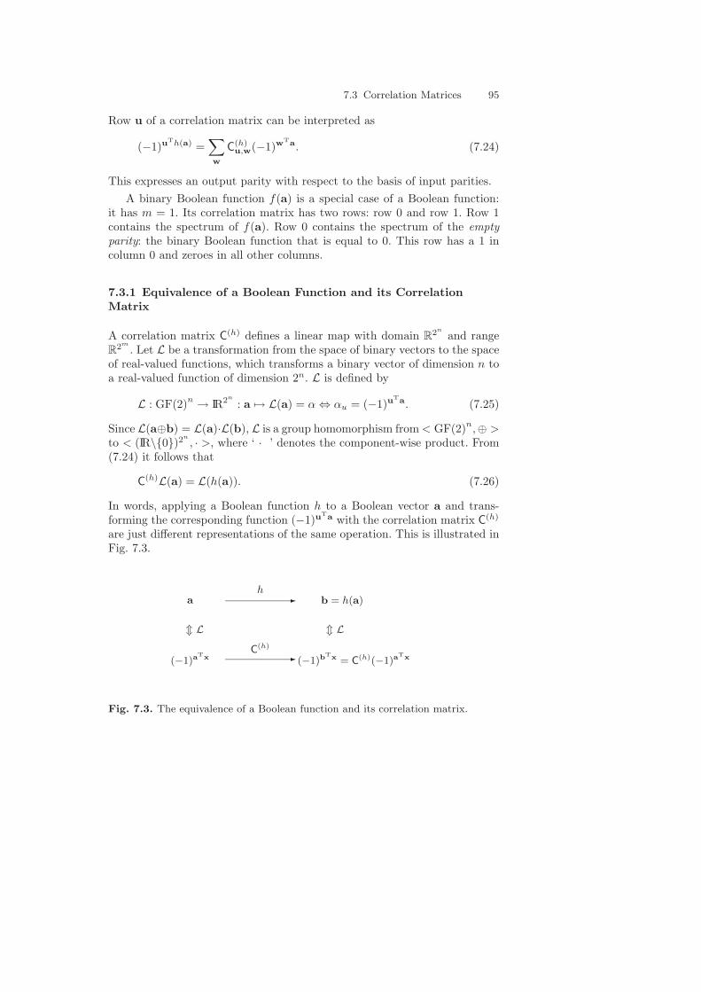
A large part of this book is aimed at the readers who want to know whywe designed Rijndael in the way we did. For them, we explain the ideas andprinciples underlying the design of Rijndael, culminating in our wide traildesign strategy. In Chap. 5 we explain our approach to block cipher designand the criteria that played an important role in the design of Rijndael. Ourdesign strategy has grown out of our experiences with linear and differentialcryptanalysis, two cryptanalytical attacks that have been applied with somesuccess to the previous standard, the Data Encryption Standard (DES). InChap. 6 we give a short overview of the DES and of the differential andthe linear attacks that are applied to it. Our framework to describe linearcryptanalysis is explained in Chap. 7; differential cryptanalysis is described

VIII Preface

in Chap. 8. Finally, in Chap. 9, we explain how the wide trail design strategyfollows from these considerations

Chapter 10 gives an overview of the published attacks on reduced-roundvariants of Rijndael. Chapter 11 gives an overview of ciphers related toRijndael. We describe its predecessors and discuss their similarities and dif-ferences. This is followed by a short description of a number of block ciphersthat have been strongly influenced by Rijndael and its predecessors.

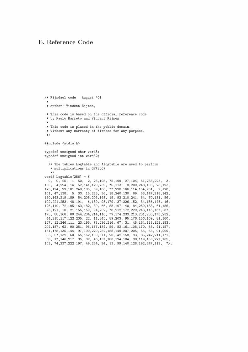
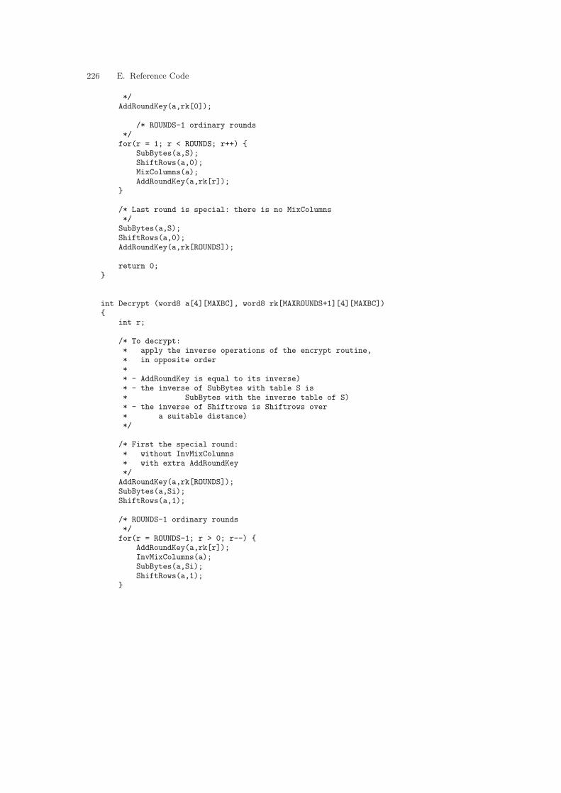
In Appendix A we show how linear and differential analysis can be appliedto ciphers that are defined in terms of finite field operations rather thanBoolean functions. In Appendix B we discuss extensions of differential andlinear cryptanalysis. To assist programmers, Appendix C lists some tablesthat are used in various descriptions of Rijndael, Appendix D gives a setof test vectors, and Appendix E consists of an example implementation ofRijndael in the C programming language.

See Fig. 1 for a graphical representation of the different ways to read thisbook.

1

2

5 6 7 8 9

3

4

10

11

�

� � � � � �

��

�

Fig. 1. Logical dependence of the chapters.

Large portions of this book have already been published before: Joan’sPhD thesis [18], Vincent’s PhD thesis [80], our submission to AES [26], andour paper on linear frameworks for block ciphers [22].

Acknowledgements

This book would not have been written without the support and help ofmany people. It is impossible for us to list all people who contributed alongthe way. Although we probably will make oversights, we would like to namesome of our supporters here.

First of all, we would like to thank the many cryptographers who con-tributed to developing the theory on the design of symmetric ciphers, andfrom who we learned much of what we know today. We would like to mentionexplicitly the people who gave us feedback in the early stages of the design

Preface IX

process: Johan Borst, Antoon Bosselaers, Paulo Barreto, Craig Clapp, ErikDe Win, Lars R. Knudsen, and Bart Preneel.

Elaine Barker, James Foti and Miles Smid, and all the other people atNIST, who worked very hard to make the AES process possible and visible.

The moral support of our family and friends, without whom we wouldnever have persevered.

Brian Gladman, who provided test vectors.Othmar Staffelbach, Elisabeth Oswald, Lee McCulloch and other proof-

readers who provided very valuable feedback and corrected numerous errorsand oversights.

The financial support of K.U.Leuven, the Fund for Scientific Research –Flanders (Belgium), Banksys, Proton World and Cryptomathic is also greatlyappreciated.

November 2001 Joan Daemen and Vincent Rijmen

Contents

1. The Advanced Encryption Standard Process . . . . . . . . . . . . . . 11.1 In the Beginning . . . . . . . . . . . . . . . . . . . . . . . . . . . . . . . . . . . . . . . 11.2 AES: Scope and Significance . . . . . . . . . . . . . . . . . . . . . . . . . . . . . 11.3 Start of the AES Process . . . . . . . . . . . . . . . . . . . . . . . . . . . . . . . . 21.4 The First Round . . . . . . . . . . . . . . . . . . . . . . . . . . . . . . . . . . . . . . . 31.5 Evaluation Criteria . . . . . . . . . . . . . . . . . . . . . . . . . . . . . . . . . . . . . 4

1.5.1 Security . . . . . . . . . . . . . . . . . . . . . . . . . . . . . . . . . . . . . . . . . 41.5.2 Costs . . . . . . . . . . . . . . . . . . . . . . . . . . . . . . . . . . . . . . . . . . . 41.5.3 Algorithm and Implementation Characteristics . . . . . . . 4

1.6 Selection of Five Finalists . . . . . . . . . . . . . . . . . . . . . . . . . . . . . . . 51.6.1 The Second AES Conference . . . . . . . . . . . . . . . . . . . . . . . 51.6.2 The Five Finalists . . . . . . . . . . . . . . . . . . . . . . . . . . . . . . . . 6

1.7 The Second Round . . . . . . . . . . . . . . . . . . . . . . . . . . . . . . . . . . . . . 71.8 The Selection . . . . . . . . . . . . . . . . . . . . . . . . . . . . . . . . . . . . . . . . . . 7

2. Preliminaries . . . . . . . . . . . . . . . . . . . . . . . . . . . . . . . . . . . . . . . . . . . . . 92.1 Finite Fields . . . . . . . . . . . . . . . . . . . . . . . . . . . . . . . . . . . . . . . . . . . 10

2.1.1 Groups, Rings, and Fields . . . . . . . . . . . . . . . . . . . . . . . . . 102.1.2 Vector Spaces . . . . . . . . . . . . . . . . . . . . . . . . . . . . . . . . . . . . 112.1.3 Fields with a Finite Number of Elements . . . . . . . . . . . . 132.1.4 Polynomials over a Field . . . . . . . . . . . . . . . . . . . . . . . . . . 132.1.5 Operations on Polynomials . . . . . . . . . . . . . . . . . . . . . . . . 142.1.6 Polynomials and Bytes . . . . . . . . . . . . . . . . . . . . . . . . . . . . 152.1.7 Polynomials and Columns . . . . . . . . . . . . . . . . . . . . . . . . . 16

2.2 Linear Codes . . . . . . . . . . . . . . . . . . . . . . . . . . . . . . . . . . . . . . . . . . 172.2.1 Definitions . . . . . . . . . . . . . . . . . . . . . . . . . . . . . . . . . . . . . . 172.2.2 MDS codes . . . . . . . . . . . . . . . . . . . . . . . . . . . . . . . . . . . . . . 19

2.3 Boolean Functions . . . . . . . . . . . . . . . . . . . . . . . . . . . . . . . . . . . . . . 192.3.1 Bundle Partitions . . . . . . . . . . . . . . . . . . . . . . . . . . . . . . . . 202.3.2 Transpositions . . . . . . . . . . . . . . . . . . . . . . . . . . . . . . . . . . . 212.3.3 Bricklayer Functions . . . . . . . . . . . . . . . . . . . . . . . . . . . . . . 222.3.4 Iterative Boolean Transformations . . . . . . . . . . . . . . . . . . 22

2.4 Block Ciphers . . . . . . . . . . . . . . . . . . . . . . . . . . . . . . . . . . . . . . . . . . 232.4.1 Iterative Block Ciphers . . . . . . . . . . . . . . . . . . . . . . . . . . . . 24

XII Contents

2.4.2 Key-Alternating Block Ciphers . . . . . . . . . . . . . . . . . . . . . 252.5 Block Cipher Modes of Operation . . . . . . . . . . . . . . . . . . . . . . . . 27

2.5.1 Block Encryption Modes . . . . . . . . . . . . . . . . . . . . . . . . . . 272.5.2 Key-Stream Generation Modes . . . . . . . . . . . . . . . . . . . . . 272.5.3 Message Authentication Modes . . . . . . . . . . . . . . . . . . . . . 282.5.4 Cryptographic Hashing . . . . . . . . . . . . . . . . . . . . . . . . . . . . 29

2.6 Conclusions . . . . . . . . . . . . . . . . . . . . . . . . . . . . . . . . . . . . . . . . . . . . 29

3. Specification of Rijndael . . . . . . . . . . . . . . . . . . . . . . . . . . . . . . . . . . 313.1 Differences between Rijndael and the AES . . . . . . . . . . . . . . . . . 313.2 Input and Output for Encryption and Decryption . . . . . . . . . . 313.3 Structure of Rijndael . . . . . . . . . . . . . . . . . . . . . . . . . . . . . . . . . . . . 333.4 The Round Transformation . . . . . . . . . . . . . . . . . . . . . . . . . . . . . . 33

3.4.1 The SubBytes Step . . . . . . . . . . . . . . . . . . . . . . . . . . . . . . . 343.4.2 The ShiftRows Step . . . . . . . . . . . . . . . . . . . . . . . . . . . . . . 373.4.3 The MixColumns Step . . . . . . . . . . . . . . . . . . . . . . . . . . . . . 383.4.4 The Key Addition . . . . . . . . . . . . . . . . . . . . . . . . . . . . . . . . 40

3.5 The Number of Rounds . . . . . . . . . . . . . . . . . . . . . . . . . . . . . . . . . 413.6 Key Schedule . . . . . . . . . . . . . . . . . . . . . . . . . . . . . . . . . . . . . . . . . . 43

3.6.1 Design Criteria . . . . . . . . . . . . . . . . . . . . . . . . . . . . . . . . . . . 433.6.2 Selection . . . . . . . . . . . . . . . . . . . . . . . . . . . . . . . . . . . . . . . . 43

3.7 Decryption . . . . . . . . . . . . . . . . . . . . . . . . . . . . . . . . . . . . . . . . . . . . 453.7.1 Decryption for a Two-Round Rijndael Variant . . . . . . . 453.7.2 Algebraic Properties . . . . . . . . . . . . . . . . . . . . . . . . . . . . . . 463.7.3 The Equivalent Decryption Algorithm . . . . . . . . . . . . . . 48

3.8 Conclusions . . . . . . . . . . . . . . . . . . . . . . . . . . . . . . . . . . . . . . . . . . . . 50

4. Implementation Aspects . . . . . . . . . . . . . . . . . . . . . . . . . . . . . . . . . . 534.1 8-Bit Platforms . . . . . . . . . . . . . . . . . . . . . . . . . . . . . . . . . . . . . . . . 53

4.1.1 Finite Field Multiplication . . . . . . . . . . . . . . . . . . . . . . . . . 534.1.2 Encryption . . . . . . . . . . . . . . . . . . . . . . . . . . . . . . . . . . . . . . 544.1.3 Decryption . . . . . . . . . . . . . . . . . . . . . . . . . . . . . . . . . . . . . . 55

4.2 32-Bit Platforms . . . . . . . . . . . . . . . . . . . . . . . . . . . . . . . . . . . . . . . 564.3 Dedicated Hardware . . . . . . . . . . . . . . . . . . . . . . . . . . . . . . . . . . . . 59

4.3.1 Decomposition of SRD . . . . . . . . . . . . . . . . . . . . . . . . . . . . 604.3.2 Efficient Inversion in GF(28) . . . . . . . . . . . . . . . . . . . . . . . 61

4.4 Multiprocessor Platforms . . . . . . . . . . . . . . . . . . . . . . . . . . . . . . . . 614.5 Performance Figures . . . . . . . . . . . . . . . . . . . . . . . . . . . . . . . . . . . . 624.6 Conclusions . . . . . . . . . . . . . . . . . . . . . . . . . . . . . . . . . . . . . . . . . . . . 62

5. Design Philosophy . . . . . . . . . . . . . . . . . . . . . . . . . . . . . . . . . . . . . . . . 635.1 Generic Criteria in Cipher Design . . . . . . . . . . . . . . . . . . . . . . . . 63

5.1.1 Security . . . . . . . . . . . . . . . . . . . . . . . . . . . . . . . . . . . . . . . . . 635.1.2 Efficiency . . . . . . . . . . . . . . . . . . . . . . . . . . . . . . . . . . . . . . . 645.1.3 Key Agility . . . . . . . . . . . . . . . . . . . . . . . . . . . . . . . . . . . . . . 64

Contents XIII

5.1.4 Versatility . . . . . . . . . . . . . . . . . . . . . . . . . . . . . . . . . . . . . . . 645.1.5 Discussion . . . . . . . . . . . . . . . . . . . . . . . . . . . . . . . . . . . . . . . 64

5.2 Simplicity . . . . . . . . . . . . . . . . . . . . . . . . . . . . . . . . . . . . . . . . . . . . . 655.3 Symmetry . . . . . . . . . . . . . . . . . . . . . . . . . . . . . . . . . . . . . . . . . . . . . 65

5.3.1 Symmetry Across the Rounds . . . . . . . . . . . . . . . . . . . . . . 665.3.2 Symmetry Within the Round Transformation . . . . . . . . 665.3.3 Symmetry in the D-box . . . . . . . . . . . . . . . . . . . . . . . . . . . 675.3.4 Symmetry and Simplicity in the S-box . . . . . . . . . . . . . . 685.3.5 Symmetry between Encryption and Decryption . . . . . . 685.3.6 Additional Benefits of Symmetry . . . . . . . . . . . . . . . . . . . 68

5.4 Choice of Operations . . . . . . . . . . . . . . . . . . . . . . . . . . . . . . . . . . . . 695.4.1 Arithmetic Operations . . . . . . . . . . . . . . . . . . . . . . . . . . . . 705.4.2 Data-Dependent Shifts . . . . . . . . . . . . . . . . . . . . . . . . . . . . 70

5.5 Approach to Security . . . . . . . . . . . . . . . . . . . . . . . . . . . . . . . . . . . 715.5.1 Security Goals . . . . . . . . . . . . . . . . . . . . . . . . . . . . . . . . . . . 715.5.2 Unknown Attacks Versus Known Attacks . . . . . . . . . . . . 725.5.3 Provable Security Versus Provable Bounds . . . . . . . . . . . 73

5.6 Approaches to Design . . . . . . . . . . . . . . . . . . . . . . . . . . . . . . . . . . . 735.6.1 Non-Linearity and Diffusion Criteria . . . . . . . . . . . . . . . . 735.6.2 Resistance against Differential and Linear Cryptanalysis 735.6.3 Local Versus Global Optimization . . . . . . . . . . . . . . . . . . 74

5.7 Key-Alternating Cipher Structure . . . . . . . . . . . . . . . . . . . . . . . . 765.8 The Key Schedule . . . . . . . . . . . . . . . . . . . . . . . . . . . . . . . . . . . . . . 76

5.8.1 The Function of a Key Schedule . . . . . . . . . . . . . . . . . . . . 765.8.2 Key Expansion and Key Selection . . . . . . . . . . . . . . . . . . 775.8.3 The Cost of the Key Expansion . . . . . . . . . . . . . . . . . . . . 775.8.4 A Recursive Key Expansion . . . . . . . . . . . . . . . . . . . . . . . 78

5.9 Conclusions . . . . . . . . . . . . . . . . . . . . . . . . . . . . . . . . . . . . . . . . . . . . 79

6. The Data Encryption Standard . . . . . . . . . . . . . . . . . . . . . . . . . . . 816.1 The DES . . . . . . . . . . . . . . . . . . . . . . . . . . . . . . . . . . . . . . . . . . . . . . 816.2 Differential Cryptanalysis . . . . . . . . . . . . . . . . . . . . . . . . . . . . . . . . 836.3 Linear Cryptanalysis . . . . . . . . . . . . . . . . . . . . . . . . . . . . . . . . . . . . 856.4 Conclusions . . . . . . . . . . . . . . . . . . . . . . . . . . . . . . . . . . . . . . . . . . . . 87

7. Correlation Matrices . . . . . . . . . . . . . . . . . . . . . . . . . . . . . . . . . . . . . 897.1 The Walsh-Hadamard Transform . . . . . . . . . . . . . . . . . . . . . . . . . 89

7.1.1 Parities and Selection Patterns . . . . . . . . . . . . . . . . . . . . . 897.1.2 Correlation . . . . . . . . . . . . . . . . . . . . . . . . . . . . . . . . . . . . . . 897.1.3 Real-valued Counterpart of a Binary Boolean Function 907.1.4 Orthogonality and Correlation . . . . . . . . . . . . . . . . . . . . . 907.1.5 Spectrum of a Binary Boolean Function . . . . . . . . . . . . . 91

7.2 Composing Binary Boolean Functions . . . . . . . . . . . . . . . . . . . . . 937.2.1 XOR . . . . . . . . . . . . . . . . . . . . . . . . . . . . . . . . . . . . . . . . . . . 937.2.2 AND . . . . . . . . . . . . . . . . . . . . . . . . . . . . . . . . . . . . . . . . . . . 93

XIV Contents

7.2.3 Disjunct Boolean Functions . . . . . . . . . . . . . . . . . . . . . . . . 947.3 Correlation Matrices . . . . . . . . . . . . . . . . . . . . . . . . . . . . . . . . . . . . 94

7.3.1 Equivalence of a Boolean Function and its CorrelationMatrix . . . . . . . . . . . . . . . . . . . . . . . . . . . . . . . . . . . . . . . . . . 95

7.3.2 Iterative Boolean Functions . . . . . . . . . . . . . . . . . . . . . . . . 967.3.3 Boolean Permutations . . . . . . . . . . . . . . . . . . . . . . . . . . . . 96

7.4 Special Boolean Functions . . . . . . . . . . . . . . . . . . . . . . . . . . . . . . . 987.4.1 XOR with a Constant . . . . . . . . . . . . . . . . . . . . . . . . . . . . . 987.4.2 Linear Functions . . . . . . . . . . . . . . . . . . . . . . . . . . . . . . . . . 987.4.3 Bricklayer Functions . . . . . . . . . . . . . . . . . . . . . . . . . . . . . . 98

7.5 Derived Properties . . . . . . . . . . . . . . . . . . . . . . . . . . . . . . . . . . . . . . 997.6 Truncating Functions . . . . . . . . . . . . . . . . . . . . . . . . . . . . . . . . . . . 1007.7 Cross-correlation and Autocorrelation . . . . . . . . . . . . . . . . . . . . . 1017.8 Linear Trails . . . . . . . . . . . . . . . . . . . . . . . . . . . . . . . . . . . . . . . . . . . 1027.9 Ciphers . . . . . . . . . . . . . . . . . . . . . . . . . . . . . . . . . . . . . . . . . . . . . . . 103

7.9.1 General Case . . . . . . . . . . . . . . . . . . . . . . . . . . . . . . . . . . . . 1037.9.2 Key-Alternating Cipher . . . . . . . . . . . . . . . . . . . . . . . . . . . 1047.9.3 Averaging over all Round Keys . . . . . . . . . . . . . . . . . . . . . 1057.9.4 The Effect of the Key Schedule . . . . . . . . . . . . . . . . . . . . . 106

7.10 Correlation Matrices and Linear Cryptanalysis Literature . . . . 1087.10.1 Linear Cryptanalysis of the DES . . . . . . . . . . . . . . . . . . . 1087.10.2 Linear Hulls . . . . . . . . . . . . . . . . . . . . . . . . . . . . . . . . . . . . . 109

7.11 Conclusions . . . . . . . . . . . . . . . . . . . . . . . . . . . . . . . . . . . . . . . . . . . . 111

8. Difference Propagation . . . . . . . . . . . . . . . . . . . . . . . . . . . . . . . . . . . 1138.1 Difference Propagation . . . . . . . . . . . . . . . . . . . . . . . . . . . . . . . . . . 1138.2 Special Functions . . . . . . . . . . . . . . . . . . . . . . . . . . . . . . . . . . . . . . . 114

8.2.1 Affine Functions . . . . . . . . . . . . . . . . . . . . . . . . . . . . . . . . . . 1148.2.2 Bricklayer Functions . . . . . . . . . . . . . . . . . . . . . . . . . . . . . . 1148.2.3 Truncating Functions . . . . . . . . . . . . . . . . . . . . . . . . . . . . . 115

8.3 Difference Propagation Probabilities and Correlation . . . . . . . . 1158.4 Differential Trails . . . . . . . . . . . . . . . . . . . . . . . . . . . . . . . . . . . . . . . 117

8.4.1 General Case . . . . . . . . . . . . . . . . . . . . . . . . . . . . . . . . . . . . 1178.4.2 Independence of Restrictions . . . . . . . . . . . . . . . . . . . . . . . 117

8.5 Key-Alternating Cipher . . . . . . . . . . . . . . . . . . . . . . . . . . . . . . . . . 1188.6 The Effect of the Key Schedule . . . . . . . . . . . . . . . . . . . . . . . . . . . 1198.7 Differential Trails and Differential Cryptanalysis Literature . . 119

8.7.1 Differential Cryptanalysis of the DES Revisited . . . . . . 1198.7.2 Markov Ciphers . . . . . . . . . . . . . . . . . . . . . . . . . . . . . . . . . . 120

8.8 Conclusions . . . . . . . . . . . . . . . . . . . . . . . . . . . . . . . . . . . . . . . . . . . . 122

Contents XV

9. The Wide Trail Strategy . . . . . . . . . . . . . . . . . . . . . . . . . . . . . . . . . . 1239.1 Propagation in Key-alternating Block Ciphers . . . . . . . . . . . . . . 123

9.1.1 Linear Cryptanalysis . . . . . . . . . . . . . . . . . . . . . . . . . . . . . . 1239.1.2 Differential Cryptanalysis . . . . . . . . . . . . . . . . . . . . . . . . . 1259.1.3 Differences between Linear Trails and Differential Trails126

9.2 The Wide Trail Strategy . . . . . . . . . . . . . . . . . . . . . . . . . . . . . . . . 1269.2.1 The γλ Round Structure in Block Ciphers . . . . . . . . . . . 1279.2.2 Weight of a Trail . . . . . . . . . . . . . . . . . . . . . . . . . . . . . . . . . 1299.2.3 Diffusion . . . . . . . . . . . . . . . . . . . . . . . . . . . . . . . . . . . . . . . . 130

9.3 Branch Numbers and Two-Round Trails . . . . . . . . . . . . . . . . . . . 1319.3.1 Derived Properties . . . . . . . . . . . . . . . . . . . . . . . . . . . . . . . 1339.3.2 A Two-Round Propagation Theorem . . . . . . . . . . . . . . . . 133

9.4 An Efficient Key-Alternating Structure . . . . . . . . . . . . . . . . . . . . 1349.4.1 The Diffusion Step θ . . . . . . . . . . . . . . . . . . . . . . . . . . . . . . 1349.4.2 The Linear Step Θ . . . . . . . . . . . . . . . . . . . . . . . . . . . . . . . 1369.4.3 A Lower Bound on the Bundle Weight of Four-Round

Trails . . . . . . . . . . . . . . . . . . . . . . . . . . . . . . . . . . . . . . . . . . . 1369.4.4 An Efficient Construction for Θ . . . . . . . . . . . . . . . . . . . . 137

9.5 The Round Structure of Rijndael . . . . . . . . . . . . . . . . . . . . . . . . . 1389.5.1 A Key-Iterated Structure . . . . . . . . . . . . . . . . . . . . . . . . . . 1389.5.2 Applying the Wide Trail Strategy to Rijndael . . . . . . . . 142

9.6 Constructions for θ . . . . . . . . . . . . . . . . . . . . . . . . . . . . . . . . . . . . . 1439.7 Choices for the Structure of I and π . . . . . . . . . . . . . . . . . . . . . . 145

9.7.1 The Hypercube Structure . . . . . . . . . . . . . . . . . . . . . . . . . 1459.7.2 The Rectangular Structure . . . . . . . . . . . . . . . . . . . . . . . . 147

9.8 Conclusions . . . . . . . . . . . . . . . . . . . . . . . . . . . . . . . . . . . . . . . . . . . . 147

10. Cryptanalysis . . . . . . . . . . . . . . . . . . . . . . . . . . . . . . . . . . . . . . . . . . . . . 14910.1 Truncated Differentials . . . . . . . . . . . . . . . . . . . . . . . . . . . . . . . . . . 14910.2 Saturation Attacks . . . . . . . . . . . . . . . . . . . . . . . . . . . . . . . . . . . . . 149

10.2.1 Preliminaries . . . . . . . . . . . . . . . . . . . . . . . . . . . . . . . . . . . . 15010.2.2 The Basic Attack . . . . . . . . . . . . . . . . . . . . . . . . . . . . . . . . . 15010.2.3 Influence of the Final Round . . . . . . . . . . . . . . . . . . . . . . . 15210.2.4 Extension at the End . . . . . . . . . . . . . . . . . . . . . . . . . . . . . 15310.2.5 Extension at the Beginning . . . . . . . . . . . . . . . . . . . . . . . . 15310.2.6 Attacks on Six Rounds . . . . . . . . . . . . . . . . . . . . . . . . . . . . 15310.2.7 The Herds Attack . . . . . . . . . . . . . . . . . . . . . . . . . . . . . . . . 154

10.3 Gilbert–Minier Attack . . . . . . . . . . . . . . . . . . . . . . . . . . . . . . . . . . 15410.3.1 The Four-Round Distinguisher . . . . . . . . . . . . . . . . . . . . . 15410.3.2 The Attack on Seven Rounds . . . . . . . . . . . . . . . . . . . . . . 155

10.4 Interpolation Attacks . . . . . . . . . . . . . . . . . . . . . . . . . . . . . . . . . . . 15610.5 Symmetry Properties and Weak Keys as in the DES . . . . . . . . 15610.6 Weak keys as in IDEA . . . . . . . . . . . . . . . . . . . . . . . . . . . . . . . . . . 15710.7 Related-Key Attacks . . . . . . . . . . . . . . . . . . . . . . . . . . . . . . . . . . . . 15710.8 Implementation Attacks . . . . . . . . . . . . . . . . . . . . . . . . . . . . . . . . . 157

XVI Contents

10.8.1 Timing Attacks . . . . . . . . . . . . . . . . . . . . . . . . . . . . . . . . . . 15710.8.2 Power Analysis . . . . . . . . . . . . . . . . . . . . . . . . . . . . . . . . . . . 158

10.9 Conclusion . . . . . . . . . . . . . . . . . . . . . . . . . . . . . . . . . . . . . . . . . . . . 160

11. Related Block Ciphers . . . . . . . . . . . . . . . . . . . . . . . . . . . . . . . . . . . . 16111.1 Overview . . . . . . . . . . . . . . . . . . . . . . . . . . . . . . . . . . . . . . . . . . . . . . 161

11.1.1 Evolution . . . . . . . . . . . . . . . . . . . . . . . . . . . . . . . . . . . . . . . 16111.1.2 The Round Transformation . . . . . . . . . . . . . . . . . . . . . . . . 162

11.2 SHARK . . . . . . . . . . . . . . . . . . . . . . . . . . . . . . . . . . . . . . . . . . . . . . . 16311.3 Square . . . . . . . . . . . . . . . . . . . . . . . . . . . . . . . . . . . . . . . . . . . . . . . . 16511.4 BKSQ . . . . . . . . . . . . . . . . . . . . . . . . . . . . . . . . . . . . . . . . . . . . . . . . 16811.5 Children of Rijndael . . . . . . . . . . . . . . . . . . . . . . . . . . . . . . . . . . . . 171

11.5.1 Crypton . . . . . . . . . . . . . . . . . . . . . . . . . . . . . . . . . . . . . . . . . 17111.5.2 Twofish . . . . . . . . . . . . . . . . . . . . . . . . . . . . . . . . . . . . . . . . . 17211.5.3 Anubis . . . . . . . . . . . . . . . . . . . . . . . . . . . . . . . . . . . . . . . . . 17211.5.4 Grand Cru . . . . . . . . . . . . . . . . . . . . . . . . . . . . . . . . . . . . . 17311.5.5 Hierocrypt . . . . . . . . . . . . . . . . . . . . . . . . . . . . . . . . . . . . . . 173

11.6 Conclusion . . . . . . . . . . . . . . . . . . . . . . . . . . . . . . . . . . . . . . . . . . . . 173

A. Propagation Analysis in Galois Fields . . . . . . . . . . . . . . . . . . . . . 175A.1 Functions over GF(2n) . . . . . . . . . . . . . . . . . . . . . . . . . . . . . . . . . . 176

A.1.1 Difference Propagation . . . . . . . . . . . . . . . . . . . . . . . . . . . . 177A.1.2 Correlation . . . . . . . . . . . . . . . . . . . . . . . . . . . . . . . . . . . . . . 177A.1.3 Functions that are Linear over GF(2n) . . . . . . . . . . . . . . 179A.1.4 Functions that are Linear over GF(2) . . . . . . . . . . . . . . . 180

A.2 Functions over (GF(2n))� . . . . . . . . . . . . . . . . . . . . . . . . . . . . . . . . 181A.2.1 Difference Propagation . . . . . . . . . . . . . . . . . . . . . . . . . . . . 182A.2.2 Correlation . . . . . . . . . . . . . . . . . . . . . . . . . . . . . . . . . . . . . . 182A.2.3 Functions that are Linear over GF(2n) . . . . . . . . . . . . . . 182A.2.4 Functions that are Linear over GF(2) . . . . . . . . . . . . . . . 183

A.3 Representations of GF(pn) . . . . . . . . . . . . . . . . . . . . . . . . . . . . . . . 184A.3.1 Cyclic Representation of GF(pn) . . . . . . . . . . . . . . . . . . . 184A.3.2 Vector Space Representation of GF(pn) . . . . . . . . . . . . . 184A.3.3 Dual Bases . . . . . . . . . . . . . . . . . . . . . . . . . . . . . . . . . . . . . . 185

A.4 Boolean Functions and Functions in GF(2n) . . . . . . . . . . . . . . . 186A.4.1 Differences in GF(2)n and GF(2n) . . . . . . . . . . . . . . . . . . 186A.4.2 Relationship Between Trace Patterns and Selection

Patterns . . . . . . . . . . . . . . . . . . . . . . . . . . . . . . . . . . . . . . . . 187A.4.3 Relationship Between Linear Functions in GF(p)n and

GF(pn) . . . . . . . . . . . . . . . . . . . . . . . . . . . . . . . . . . . . . . . . . 187A.4.4 Illustration . . . . . . . . . . . . . . . . . . . . . . . . . . . . . . . . . . . . . . 190

A.5 Rijndael-GF . . . . . . . . . . . . . . . . . . . . . . . . . . . . . . . . . . . . . . . . . . . 192

Contents XVII

B. Trail Clustering . . . . . . . . . . . . . . . . . . . . . . . . . . . . . . . . . . . . . . . . . . . 195B.1 Transformations with Maximum Branch Number . . . . . . . . . . . 196B.2 Bounds for Two Rounds . . . . . . . . . . . . . . . . . . . . . . . . . . . . . . . . . 199

B.2.1 Difference Propagation . . . . . . . . . . . . . . . . . . . . . . . . . . . . 200B.2.2 Correlation . . . . . . . . . . . . . . . . . . . . . . . . . . . . . . . . . . . . . . 202

B.3 Bounds for Four Rounds . . . . . . . . . . . . . . . . . . . . . . . . . . . . . . . . 204B.4 Two Case Studies . . . . . . . . . . . . . . . . . . . . . . . . . . . . . . . . . . . . . . 205

B.4.1 Differential Trails . . . . . . . . . . . . . . . . . . . . . . . . . . . . . . . . . 205B.4.2 Linear Trails . . . . . . . . . . . . . . . . . . . . . . . . . . . . . . . . . . . . . 207

C. Substitution Tables . . . . . . . . . . . . . . . . . . . . . . . . . . . . . . . . . . . . . . . 211C.1 SRD . . . . . . . . . . . . . . . . . . . . . . . . . . . . . . . . . . . . . . . . . . . . . . . . . . 211C.2 Other Tables . . . . . . . . . . . . . . . . . . . . . . . . . . . . . . . . . . . . . . . . . . . 212

C.2.1 xtime . . . . . . . . . . . . . . . . . . . . . . . . . . . . . . . . . . . . . . . . . . . 212C.2.2 Round Constants . . . . . . . . . . . . . . . . . . . . . . . . . . . . . . . . . 212

D. Test Vectors . . . . . . . . . . . . . . . . . . . . . . . . . . . . . . . . . . . . . . . . . . . . . . 215D.1 KeyExpansion . . . . . . . . . . . . . . . . . . . . . . . . . . . . . . . . . . . . . . . . . 215D.2 Rijndael(128,128) . . . . . . . . . . . . . . . . . . . . . . . . . . . . . . . . . . . . . . . 215D.3 Other Block Lengths and Key Lengths . . . . . . . . . . . . . . . . . . . . 217

E. Reference Code . . . . . . . . . . . . . . . . . . . . . . . . . . . . . . . . . . . . . . . . . . . 221

Bibliography . . . . . . . . . . . . . . . . . . . . . . . . . . . . . . . . . . . . . . . . . . . . . . . . . . 229

Index . . . . . . . . . . . . . . . . . . . . . . . . . . . . . . . . . . . . . . . . . . . . . . . . . . . . . . . . . 235

1. The Advanced Encryption Standard Process

The main subject of this book would probably have remained an esoteric topicof cryptographic research — with a name unpronounceable to most of theworld — without the Advanced Encryption Standard (AES) process. There-fore, we thought it proper to include a short overview of the AES process.

1.1 In the Beginning . . .

In January 1997, the US National Institute of Standards and Technology(NIST) announced the start of an initiative to develop a new encryptionstandard: the AES. The new encryption standard was to become a FederalInformation Processing Standard (FIPS), replacing the old Data EncryptionStandard (DES) and triple-DES.

Unlike the selection process for the DES, the Secure Hash Algorithm(SHA-1) and the Digital Signature Algorithm (DSA), NIST had announcedthat the AES selection process would be open. Anyone could submit a can-didate cipher. Each submission, provided it met the requirements, would beconsidered on its merits. NIST would not perform any security or efficiencyevaluation itself, but instead invited the cryptology community to mountattacks and try to cryptanalyse the different candidates, and anyone whowas interested to evaluate implementation cost. All results could be sent toNIST as public comments for publication on the NIST AES web site or besubmitted for presentation at AES conferences. NIST would merely collectcontributions using them to base their selection. NIST would motivate theirchoices in evaluation reports.

1.2 AES: Scope and Significance

The official scope of a FIPS standard is quite limited: the FIPS only appliesto the US Federal Administration. Furthermore, the new AES would onlybe used for documents that contain sensitive but not classified information.

2 1. The Advanced Encryption Standard Process

However, it was anticipated that the impact of the AES would be much largerthan this: for AES is the successor of the DES, the cipher that ever since itsadoption has been used as a worldwide de facto cryptographic standard bybanks, administrations and industry.

Rijndael’s approval as a government standard gives it an official ‘certifi-cate of quality’. AES has been submitted to the International Organizationfor Standardization (ISO) and the Internet Engineering Task Force (IETF)as well as the Institute of Electrical and Electronics Engineers (IEEE) areadopting it as a standard. Still, even before Rijndael was selected to be-come the AES, several organizations and companies declared their adoptionof Rijndael. The European Telecommunications Standards Institute (ETSI)uses Rijndael as a building block for its MILENAGE algorithm set, and sev-eral vendors of cryptographic libraries had already included Rijndael in theirproducts.

The major factors for a quick acceptance for Rijndael are the fact thatit is available royalty-free, and that it can be implemented easily on a widerange of platforms without reducing bandwidth in a significant way.

1.3 Start of the AES Process

In September 1997, the final request for candidate nominations for the AESwas published. The minimum functional requirements asked for symmetricblock ciphers capable of supporting block lengths of 128 bits and key lengthsof 128, 192 and 256 bits. An early draft of the AES functional requirementshad asked for block ciphers also supporting block sizes of 192 and 256 bits,but this requirement was dropped later on. Nevertheless, since the requestfor proposals mentioned that extra functionality in the submissions wouldbe received favourably, some submitters decided to keep the variable blocklength in the designs. (Examples include RC6 and Rijndael.)

NIST declared that it was looking for a block cipher as secure as triple-DES, but much more efficient. Another mandatory requirement was that thesubmitters agreed to make their cipher available on a world wide royalty-freebasis, if it would be selected as the AES. In order to qualify as an officialAES candidate, the designers had to provide:

1. A complete written specification of the block cipher in the form of analgorithm.

2. A reference implementation in ANSI C, and mathematically optimizedimplementations in ANSI C and Java.

3. Implementations of a series of known-answer and Monte Carlo tests, aswell as the expected outputs of these tests for a correct implementationof their block cipher.

1.4 The First Round 3

4. Statements concerning the estimated computational efficiency in bothhardware and software, the expected strength against cryptanalytic at-tacks, and the advantages and limitations of the cipher in various appli-cations.

5. An analysis of the cipher’s strength against known cryptanalytic attacks.

It turned out that the required effort to produce a ‘complete and proper’submission package would already filter out several of the proposals. Early inthe submission stage, the Cryptix team announced that they would provideJava implementations for all submitted ciphers, as well as Java implementa-tions of the known-answer and Monte Carlo tests. This generous offer tooksome weight off the designers’ shoulders, but still the effort required to com-pile a submission package was too heavy for some designers. The fact thatthe AES Application Programming Interface (API), which all submissionswere required to follow, was updated two times during the submission stage,increased the workload. Table 1.1 lists (in alphabetical order) the 15 submis-sions that were completed in time and accepted.

Table 1.1. The 15 AES candidates accepted for the first evaluation round.

Submissions Submitter(s) Submitter type

CAST-256 Entrust (CA) Company

Crypton Future Systems (KR) Company

DEAL Outerbridge, Knudsen (USA–DK) Researchers

DFC ENS-CNRS (FR) Researchers

E2 NTT (JP) Company

Frog TecApro (CR) Company

HPC Schroeppel (USA) Researcher

LOKI97 Brown et al. (AU) Researchers

Magenta Deutsche Telekom (DE) Company

Mars IBM (USA) Company

RC6 RSA (USA) Company

Rijndael Daemen and Rijmen (BE) Researchers

SAFER+ Cylink (USA) Company

Serpent Anderson, Biham, Knudsen (UK–IL–DK) Researchers

Twofish Counterpane (USA) Company

1.4 The First Round

The selection process was divided into several stages, with a public workshopto be held near the end of each stage. The process started with a submission


stage, which ended on 15 May 1998. All accepted candidates were presentedat The First Advanced Encryption Standard Candidate conference, held inVentura, California, on 20-22 August 1998. This was the official start of thefirst evaluation round, during which the international cryptographic commu-nity was asked for comments on the candidates.

1.5 Evaluation Criteria

The evaluation criteria for the first round were divided into three major cate-gories: security, cost and algorithm and implementation characteristics. NISTinvited the cryptology community to mount attacks and try to cryptanalysethe different candidates, and anyone interested to evaluate implementationcost. The result could be sent to NIST as public comments or be submittedfor presentation at the second AES conference. NIST collected all contribu-tions and would use these to select five finalists. In the following sections wediscuss the evaluation criteria.

1.5.1 Security

Security was the most important category, but perhaps the most difficultto assess. Only a small number of candidates showed some theoretical designflaws. The large majority of the candidates fell into the category ‘no weaknessdemonstrated’.

1.5.2 Costs

The ‘costs’ of the candidates were divided into different subcategories. A firstcategory was formed by costs associated with intellectual property (IP) issues.First of all, each submitter was required to make his cipher available for freeif it would be selected as the AES. Secondly, each submitter was also askedto make a signed statement that he would not claim ownership or exercisepatents on ideas used in another submitter’s proposal that would eventuallybe selected as AES. A second category of ‘costs’ was formed by costs asso-ciated with the implementation and execution of the candidates. This coversaspects such as computational efficiency, program size and working memoryrequirements in software implementations, and chip area in dedicated hard-ware implementations.

1.5.3 Algorithm and Implementation Characteristics

The category algorithm and implementation characteristics grouped a num-ber of features that are harder to quantify. The first one is versatility, meaning

1.6 Selection of Five Finalists 5

the ability to be implemented efficiently on different platforms. At one endof the spectrum should the AES fit 8-bit micro-controllers and smart cards,which have limited storage for the program and a very restricted amount ofRAM for working memory. At the other end of the spectrum the AES shouldbe implementable efficiently in dedicated hardware, e.g. to provide on-the-flyencryption/decryption of communication links at gigabit-per-second rates. Inbetween there is the whole range of processors that are used in servers, work-stations, PCs, palmtops etc., which are all devices in need of cryptographicsupport. A prominent place in this range is taken by the Pentium family ofprocessors due to its presence in most personal computers.

A second feature is key agility. In most block ciphers, key set up takessome processing. In applications where the same key is used to encrypt largeamounts of data, this processing is relatively unimportant. In applicationswhere the key often changes, such as the encryption of Internet Protocol(IP) packets in Internet Protocol Security (IPSEC), the overhead due to keysetup may become quite relevant. Obviously, in those applications it is anadvantage to have a fast key setup.

Finally, there is the criterion of simplicity, that may even be harder toevaluate than cryptographic security. Simplicity is related to the size of thedescription, the number of different operations used in the specification, sym-metry or lack of symmetry in the cipher and the ease with which the algo-rithm can be understood. All other things equal, NIST considered it to bean advantage for an AES candidate to be more simple for reasons of ease ofimplementation and confidence in security.

1.6 Selection of Five Finalists

In March 1999, the second AES conference was held in Rome, Italy. Theremarkable fact that a US Government department organized a conferenceon a future US Standard in Europe is easily explained. NIST chose to combinethe conference with the yearly Fast Software Encryption Workshop that hadfor the most part the same target audience and that was scheduled to be inRome.

1.6.1 The Second AES Conference

The papers presented at the conference ranged from crypto-attacks, ciphercross-analysis, smart-card-related papers, and so-called algorithm observa-tions. In the session on cryptographic attacks, it was shown that FROG,Magenta and LOKI97 did not satisfy the security requirements imposed byNIST. For DEAL it was already known in advance that that the security re-quirements were not satisfied. For HPC weaknesses had been demonstratedin a paper previously sent to NIST. This eliminated five candidates.


Some cipher cross-analysis papers focused on performance evaluation. Thepaper of B. Gladman [37], a researcher who had no link with any submission,considered performance on the Pentium processor. From this paper it becameclear that RC6, Rijndael, Twofish, MARS and Crypton where the five fastestciphers on this processor. On the other hand, the candidates DEAL, Frog,Magenta, SAFER+ and Serpent appeared to be problematically slow. Otherpapers by the Twofish team (Bruce Schneier et al.) [84] and a French teamof 12 cryptographers [5] essentially confirmed this.

A paper by E. Biham warned that the security margins of the AES can-didates differed greatly and that this should be taken into account in theperformance evaluation [7]. The lack of speed of Serpent (with E. Biham inthe design team) was seen to be compensated with a very high margin of se-curity. Discussions on how to measure and take into account security marginslasted until after the third AES conference.

In the session on smart cards there were two papers comparing the perfor-mance of AES candidates on typical 8-bit processors and a 32-bit processor:one by G. Keating [48] and one by G. Hachez et al. [40]. From these papersand results from other papers, it became clear that some candidates simplydo not fit into a smart card and that Rijndael is by far the best suited for thisplatform. In the same session there were some papers that discussed poweranalysis attacks and the suitability of the different candidates for implemen-tations that can resist against these attacks [10, 15, 27].

Finally, in the algorithm observations session, there were a number ofpapers in which AES submitters re-confirmed their confidence in their sub-mission by means of a considerable amount of formulas, graphs and tables andsome loyal cryptanalysis (the demonstration of having found no weaknessesafter attacks of its own cipher).

1.6.2 The Five Finalists

After the workshop there was a relatively calm period that ended with theannouncement of the five candidates by NIST in August 1999. The finalistswere (in alphabetical order): MARS, RC6, Rijndael, Serpent and Twofish.

Along with the announcement of the finalists, NIST published a statusreport [72] in which the selection was motivated. The choice coincided withthe top five that resulted from the response to a questionnaire handed outat the end of the second AES workshop. Despite its moderate performance,Serpent made it thanks to its high security margin. The candidates that hadnot been eliminated because of security problems were not selected mainlyfor the following reasons:

1. CAST-256: comparable to Serpent but with a higher implementationcost.

1.7 The Second Round 7

2. Crypton: comparable to Rijndael and Twofish but with a lower securitymargin.

3. DFC: low security margin and bad performance on anything other than64-bit processors.

4. E2: comparable to Rijndael and Twofish in structure, but with a lowersecurity margin and higher implementation cost.

5. SAFER+: high security margin similar to Serpent but even slower.

1.7 The Second Round

After the announcement of the five candidates NIST made another open callfor contributions focused on the finalists. Intellectual property issues andperformance and chip area in dedicated hardware implementations enteredthe picture. A remarkable contribution originated from NSA, presenting theresults of hardware performance simulations performed for the finalists. Thisthird AES conference was held in New York City in April 2000. As in theyear before, it was combined with the Fast Software Encryption Workshop.

In the sessions on cryptographic attacks there were some interesting re-sults but no breakthroughs, since none of the finalists showed any weak-nesses that could jeopardize their security. Most of the results were attackson reduced-round versions of the ciphers. All attacks presented are only ofacademic relevance in that they are only slightly faster than an exhaustivekey search. In the sessions on software implementations, the conclusions ofthe second workshop were confirmed.

In the sessions on dedicated hardware implementations there was atten-tion for Field Programmable Gate Arrays (FPGAs) and Application-SpecificIntegrated Circuits (ASICs). In the papers Serpent came out as a consistentlyexcellent performer. Rijndael and Twofish also proved to be quite suited forhardware implementation while RC6 turned out to be expensive due to itsuse of 32-bit multiplication. Dedicated hardware implementations of MARSseemed in general to be quite costly. The Rijndael related results presented atthis conference are discussed in more detail in Chap. 4 (which is on efficientimplementations) and Chap. 10 (which is on cryptanalytic results).

At the end of the conference a questionnaire was handed out asking aboutthe preferences of the attendants. Rijndael resoundingly voted as the public’sfavourite.

1.8 The Selection

On 2 October, 2000, NIST officially announced that Rijndael, without modifi-cations, would become the AES. NIST published an excellent 116-page report


in which they summarize all contributions and motivate the choice [71]. Inthe conclusion of this report, NIST motivates the choice of Rijndael with thefollowing words.

Rijndael appears to be consistently a very good performer in bothhardware and software across a wide range of computing environ-ments regardless of its use in feedback or non-feedback modes. Itskey setup time is excellent, and its key agility is good. Rijndael’svery low memory requirements make it very well suited for restricted-space environments, in which it also demonstrates excellent perfor-mance. Rijndael’s operations are among the easiest to defend againstpower and timing attacks. Additionally, it appears that some defensecan be provided against such attacks without significantly impactingRijndael’s performance.Finally, Rijndael’s internal round structure appears to have goodpotential to benefit from instruction-level parallelism.

2. Preliminaries

In this chapter we introduce a number of mathematical concepts and explainthe terminology that we need in the specification of Rijndael (in Chap. 3),in the treatment of some implementation aspects (in Chap. 4) and when wediscuss our design choices (Chaps. 5–9).

The first part of this chapter starts with a discussion of finite fields, therepresentation of its elements and the impact of this on its operations of addi-tion and multiplication. Subsequently, there is a short introduction to linearcodes. Understanding the mathematics is not necessary for a full and correctimplementation of the cipher. However, the mathematics is necessary for agood understanding of our design motivations. Knowledge of the underlyingmathematical constructions also helps for doing optimised implementations.Not all aspects will be covered in detail; where possible, we refer to booksdedicated to the topics we introduce.

In the second part of this chapter we introduce the terminology thatwe use to indicate different common types of Boolean functions and blockciphers. Finally, we give a short overview of the modes of operation of ablock cipher.

When the discussion moves from a general level to an example specificto Rijndael, the text is put in a grey box.

Notation. We use in this book two types of indexing:

subscripts: Parts of a larger, named structure are denoted with subscripts.For instance, the bytes of a state a are denoted by ai,j (see Chap. 3).

superscripts: In an enumeration of more or less independent objects, wherethe objects are denoted by their own symbols, we use superscripts. Forinstance the elements of a nameless set are denoted by {a(1),a(2), . . .},and consecutive rounds of an iterative transformation are denoted byρ(1), ρ(2), . . . (see Sect. 2.3.4).

10 2. Preliminaries

2.1 Finite Fields

In this section we present a basic introduction to the theory of finite fields.For a more formal and elaborate introduction, we refer to the work of Lidland Niederreiter [58].

2.1.1 Groups, Rings, and Fields

We start with the formal definition of a group.

Definition 2.1.1. An Abelian group < G,+ > consists of a set G and anoperation defined on its elements, here denoted by ‘+’:

+ : G × G → G : (a, b) �→ a + b. (2.1)

In order to qualify as an Abelian group, the operation has to fulfill the fol-lowing conditions:

closed: ∀ a, b ∈ G : a + b ∈ G (2.2)associative: ∀ a, b, c ∈ G : (a + b) + c = a + (b + c) (2.3)

commutative: ∀ a, b ∈ G : a + b = b + a (2.4)neutral element: ∃0 ∈ G,∀ a ∈ G : a + 0 = a (2.5)

inverse elements: ∀ a ∈ G,∃ b ∈ G : a + b = 0 (2.6)

Example 2.1.1. The best-known example of an Abelian group is < Z,+ >:the set of integers, with the operation ‘addition’. The structure < Zn,+ > isa second example. The set contains the integer numbers 0 to n − 1 and theoperation is addition modulo n.

Since the addition of integers is the best known example of a group, usuallythe symbol ‘+’ is used to denote an arbitrary group operation. In this book,both an arbitrary group operation and integer addition will be denoted bythe symbol ‘+’. For some special types of groups, we will denote the additionoperation by the symbol ‘⊕’ (see Sect. 2.1.3).

Both rings and fields are formally defined as structures that consist of aset of elements with two operations defined on these elements.

Definition 2.1.2. A ring < R,+, · > consists of a set R with two operationsdefined on its elements, here denoted by ‘+’ and ‘·’. In order to qualify as aring, the operations have to fulfill the following conditions:

1. The structure < R,+ > is an Abelian group.2. The operation ‘·’ is closed, and associative over R. There is a neutral

element for ‘·’ in R.

2.1 Finite Fields 11

3. The two operations ‘+’ and ‘·’ are related by the law of distributivity:

∀ a, b, c ∈ R : (a + b) · c = (a · c) + (b · c). (2.7)

The neutral element for ‘·’ is usually denoted by 1. A ring < R,+, · > iscalled a commutative ring if the operation ‘·’ is commutative.

Example 2.1.2. The best-known example of a ring is < Z,+, · >: the set ofintegers, with the operations ‘addition’ and ‘multiplication’. This ring is acommutative ring. The set of matrices with n rows and n columns, with theoperations ‘matrix addition’ and ‘matrix multiplication’ is a ring, but not acommutative ring (if n > 1).

Definition 2.1.3. A structure < F,+, · > is a field if the following twoconditions are satisfied:

1. < F,+, · > is a commutative ring.2. For all elements of F , there is an inverse element in F with respect to the

operation ‘·’, except for the element 0, the neutral element of < F,+ >.

A structure < F,+, · > is a field iff both < F,+ > and < F\{0}, · > areAbelian groups and the law of distributivity applies. The neutral element of< F\{0}, · > is called the unit element of the field.

Example 2.1.3. The best-known example of a field is the set of real num-bers, with the operations ‘addition’ and ‘multiplication.’ Other examples arethe set of complex numbers and the set of rational numbers, with the sameoperations. Note that for these examples the number of elements is infinite.

2.1.2 Vector Spaces

Let < F,+, · > be a field, with unit element 1, and let < V,+ > be anAbelian group. Let ‘�’ be an operation on elements of F and V :

� : F × V → V. (2.8)

Definition 2.1.4. The structure < F, V,+,+, ·,� > is a vector space overF if the following conditions are satisfied:

1. distributivity:

∀ a ∈ F,∀ v,w ∈ V : a � (v+w) = (a � v)+ (a � w) (2.9)∀ a, b ∈ F,∀ v ∈ V : (a + b) � v = (a � v)+ (a � v) (2.10)

2. associativity:

∀ a, b ∈ F,∀ v ∈ V : (a · b) � v = a � (b � v) (2.11)

12 2. Preliminaries

3. neutral element:

∀ v ∈ V : 1 � v = v. (2.12)

The elements of V are called vectors, and the elements of F are the scalars.The operation ‘+’ is called the vector addition, and ‘�’ is the scalar multi-plication.

Example 2.1.4. For any field F , the set of n-tuples (a0, a1, . . . , an−1) forms avector space, where ‘+’ and ‘�’ are defined in terms of the field operations:

(a1, . . . , an)+ (b1, . . . , bn) = (a1 + b1, . . . , an + bn) (2.13)a � (b1, . . . , bn) = (a · b1, . . . , a · bn). (2.14)

A vector v is a linear combination of the vectors w(1),w(2), . . . ,w(s) ifthere exist scalars a(i) such that:

v = a(1) � w(1) + a(2) � w(2) + · · · + a(s) � w(s). (2.15)

In a vector space we can always find a set of vectors such that all elements ofthe vector space can be written in exactly one way as a linear combination ofthe vectors of the set. Such a set is called a basis of the vector space. We willconsider only vector spaces where the bases have a finite number of elements.We denote a basis by

e =[e(1), e(2), . . . e(n)

]T

. (2.16)

In this expression the T superscript denotes taking te transpose of the columnvector e. The scalars used in this linear combination are called the coordinatesof x with respect to the basis e:

co(x) = x = (c1, c2, . . . , cn) ⇔ x =∑n

i=1ci � e(i). (2.17)

In order to simplify the notation, from now on we will denote vector additionby the same symbol as the field addition (‘+’), and the scalar multiplicationby the same symbol as the field multiplication (‘·’). It should always be clearfrom the context what operation the symbols are referring to.

A function f is called a linear function of a vector space V over a field F ,if it has the following properties:

∀ x,y ∈ V : f(x + y) = f(x) + f(y) (2.18)∀ a ∈ F,∀ x ∈ V : f(ax) = af(x). (2.19)

The linear functions of a vector space can be represented by a matrix multi-plication on the coordinates of the vectors. A function f is a linear functionof the vector space GF(p)n iff there exists a matrix M such that

co(f(x)) = M · x,∀ x ∈ GF(p)n. (2.20)


2.1.3 Fields with a Finite Number of Elements

A finite field is a field with a finite number of elements. The number ofelements in the set is called the order of the field. A field with order m existsiff m is a prime power, i.e. m = pn for some integer n and with p a primeinteger. p is called the characteristic of the finite field.

All finite fields used in the description of Rijndael have a characteristic of 2.By the symbol ‘⊕’, we will always denote the addition operation in a fieldwith a characteristic of 2.

Fields of the same order are isomorphic: they display exactly the samealgebraic structure differing only in the representation of the elements. Inother words, for each prime power there is exactly one finite field, denotedby GF(pn). From now on, we will only consider fields with a finite number ofelements.

Perhaps the most intuitive examples of finite fields are the fields of primeorder p. The elements of a finite field GF(p) can be represented by the integers0, 1, . . . , p − 1. The two operations of the field are then ‘integer additionmodulo p’ and ‘integer multiplication modulo p’.

For finite fields with an order that is not prime, the operations additionand multiplication cannot be represented by addition and multiplication ofintegers modulo a number. Instead, slightly more complex representationsmust be introduced. Finite fields GF(pn) with n > 1 can be represented inseveral ways. The representation of GF(pn) by means of polynomials overGF(p) is quite popular and is the one we have adopted in Rijndael and itspredecessors. In the next sections, we explain this representation.

2.1.4 Polynomials over a Field

A polynomial over a field F is an expression of the form

b(x) = bn−1xn−1 + bn−2x

n−2 + · · · + b2x2 + b1x + b0, (2.21)

x being called the indeterminate of the polynomial, and the bi ∈ F thecoefficients.

We will consider polynomials as abstract entities only, which are neverevaluated. Because the sum is never evaluated, we always use the symbol ‘+’in polynomials, even if they are defined over a field with characteristic 2.

The degree of a polynomial equals � if bj = 0,∀j > �, and � is the smallestnumber with this property. The set of polynomials over a field F is denotedby F [x]. The set of polynomials over a field F , which have a degree below �,is denoted by F [x]|�.

In computer memory, the polynomials in F [x]|� with F a finite field canbe stored efficiently by storing the � coefficients as a string.

14 2. Preliminaries

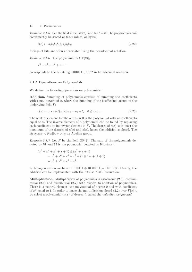
Example 2.1.5. Let the field F be GF(2), and let � = 8. The polynomials canconveniently be stored as 8-bit values, or bytes:

b(x) �→ b7b6b5b4b3b2b1b0. (2.22)

Strings of bits are often abbreviated using the hexadecimal notation.

Example 2.1.6. The polynomial in GF(2)|8x6 + x4 + x2 + x + 1

corresponds to the bit string 01010111, or 57 in hexadecimal notation.

2.1.5 Operations on Polynomials

We define the following operations on polynomials.

Addition. Summing of polynomials consists of summing the coefficientswith equal powers of x, where the summing of the coefficients occurs in theunderlying field F :

c(x) = a(x) + b(x) ⇔ ci = ai + bi, 0 ≤ i < n. (2.23)

The neutral element for the addition 0 is the polynomial with all coefficientsequal to 0. The inverse element of a polynomial can be found by replacingeach coefficient by its inverse element in F . The degree of c(x) is at most themaximum of the degrees of a(x) and b(x), hence the addition is closed. Thestructure < F [x]|�,+ > is an Abelian group.

Example 2.1.7. Let F be the field GF(2). The sum of the polynomials de-noted by 57 and 83 is the polynomial denoted by D4, since:

(x6 + x4 + x2 + x + 1) ⊕ (x7 + x + 1)= x7 + x6 + x4 + x2 + (1 ⊕ 1)x + (1 ⊕ 1)= x7 + x6 + x4 + x2.

In binary notation we have: 01010111 ⊕ 10000011 = 11010100. Clearly, theaddition can be implemented with the bitwise XOR instruction.

Multiplication. Multiplication of polynomials is associative (2.3), commu-tative (2.4) and distributive (2.7) with respect to addition of polynomials.There is a neutral element: the polynomial of degree 0 and with coefficientof x0 equal to 1. In order to make the multiplication closed (2.2) over F [x]|�,we select a polynomial m(x) of degree �, called the reduction polynomial.


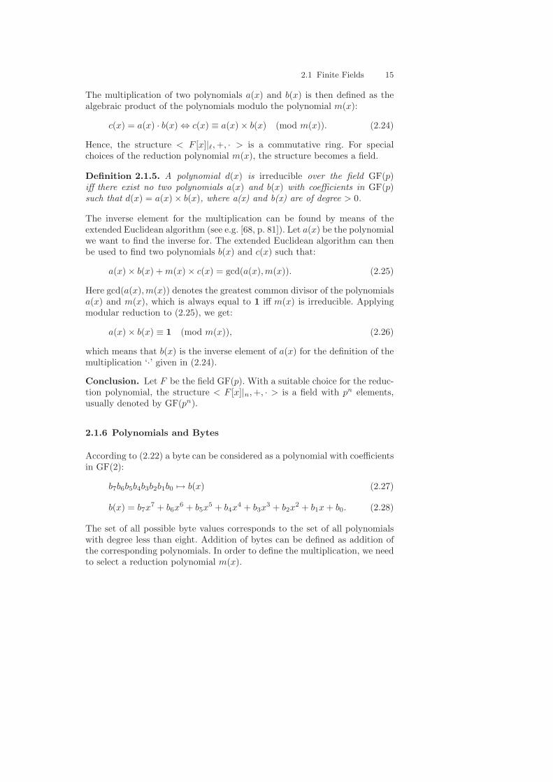
The multiplication of two polynomials a(x) and b(x) is then defined as thealgebraic product of the polynomials modulo the polynomial m(x):

c(x) = a(x) · b(x) ⇔ c(x) ≡ a(x) × b(x) (mod m(x)). (2.24)

Hence, the structure < F [x]|�,+, · > is a commutative ring. For specialchoices of the reduction polynomial m(x), the structure becomes a field.

Definition 2.1.5. A polynomial d(x) is irreducible over the field GF(p)iff there exist no two polynomials a(x) and b(x) with coefficients in GF(p)such that d(x) = a(x) × b(x), where a(x) and b(x) are of degree > 0.

The inverse element for the multiplication can be found by means of theextended Euclidean algorithm (see e.g. [68, p. 81]). Let a(x) be the polynomialwe want to find the inverse for. The extended Euclidean algorithm can thenbe used to find two polynomials b(x) and c(x) such that:

a(x) × b(x) + m(x) × c(x) = gcd(a(x),m(x)). (2.25)

Here gcd(a(x),m(x)) denotes the greatest common divisor of the polynomialsa(x) and m(x), which is always equal to 1 iff m(x) is irreducible. Applyingmodular reduction to (2.25), we get:

a(x) × b(x) ≡ 1 (mod m(x)), (2.26)

which means that b(x) is the inverse element of a(x) for the definition of themultiplication ‘·’ given in (2.24).

Conclusion. Let F be the field GF(p). With a suitable choice for the reduc-tion polynomial, the structure < F [x]|n,+, · > is a field with pn elements,usually denoted by GF(pn).

2.1.6 Polynomials and Bytes

According to (2.22) a byte can be considered as a polynomial with coefficientsin GF(2):

b7b6b5b4b3b2b1b0 �→ b(x) (2.27)

b(x) = b7x7 + b6x

6 + b5x5 + b4x

4 + b3x3 + b2x

2 + b1x + b0. (2.28)

The set of all possible byte values corresponds to the set of all polynomialswith degree less than eight. Addition of bytes can be defined as addition ofthe corresponding polynomials. In order to define the multiplication, we needto select a reduction polynomial m(x).

16 2. Preliminaries

In the specification of Rijndael, we consider the bytes as polynomials.Byte addition is defined as addition of the corresponding polynomials. Inorder to define byte multiplication, we use the following irreducible polyno-mial as reduction polynomial:

m(x) = x8 + x4 + x3 + x + 1. (2.29)

Since this reduction polynomial is irreducible, we have constructed a rep-resentation for the field GF(28). Hence we can state the following: In theRijndael specification, bytes are considered as elements of GF(28). Opera-tions on bytes are defined as operations in GF(28).

Example 2.1.8. In our representation for GF(28), the product of the elementsdenoted by 57 and 83 is the element denoted by C1, since:

(x6 + x4 + x2 + x + 1) × (x7 + x + 1)= (x13 + x11 + x9 + x8 + x7) ⊕ (x7 + x5 + x3 + x2 + x)

⊕ (x6 + x4 + x2 + x + 1)= x13 + x11 + x9 + x8 + x6 + x5 + x4 + x3 + 1

and

(x13 + x11 + x9 + x8 + x6 + x5 + x4 + x3 + 1)≡ x7 + x6 + 1 (mod x8 + x4 + x3 + x + 1).

As opposed to addition, there is no simple equivalent processor instruction.

2.1.7 Polynomials and Columns

In the Rijndael specification, 4-byte columns are considered as polyno-mials over GF(28), having a degree smaller than four. In order to define themultiplication operation, the following reduction polynomial is used:

l(x) = x4 + 1. (2.30)

This polynomial is reducible, since in GF(28)

x4 + 1 = (x + 1)4. (2.31)

In the definition of Rijndael, one of the inputs of the multiplication is aconstant polynomial.

Since l(x) is reducible over GF(28), not all polynomials have an inverseelement for the multiplication modulo l(x). A polynomial b(x) has an inverseif the polynomial x + 1 does not divide it.

2.2 Linear Codes 17

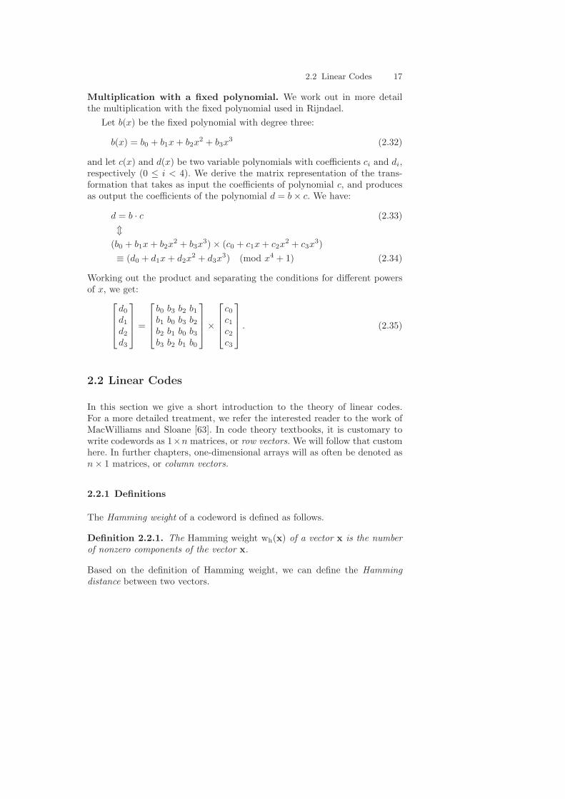
Multiplication with a fixed polynomial. We work out in more detailthe multiplication with the fixed polynomial used in Rijndael.

Let b(x) be the fixed polynomial with degree three:

b(x) = b0 + b1x + b2x2 + b3x

3 (2.32)

and let c(x) and d(x) be two variable polynomials with coefficients ci and di,respectively (0 ≤ i < 4). We derive the matrix representation of the trans-formation that takes as input the coefficients of polynomial c, and producesas output the coefficients of the polynomial d = b × c. We have:

d = b · c (2.33)�

(b0 + b1x + b2x2 + b3x

3) × (c0 + c1x + c2x2 + c3x

3)≡ (d0 + d1x + d2x

2 + d3x3) (mod x4 + 1) (2.34)

Working out the product and separating the conditions for different powersof x, we get:

d0

d1

d2

d3

=

b0 b3 b2 b1

b1 b0 b3 b2

b2 b1 b0 b3

b3 b2 b1 b0

×

c0

c1

c2

c3

. (2.35)

2.2 Linear Codes

In this section we give a short introduction to the theory of linear codes.For a more detailed treatment, we refer the interested reader to the work ofMacWilliams and Sloane [63]. In code theory textbooks, it is customary towrite codewords as 1×n matrices, or row vectors. We will follow that customhere. In further chapters, one-dimensional arrays will as often be denoted asn × 1 matrices, or column vectors.

2.2.1 Definitions

The Hamming weight of a codeword is defined as follows.

Definition 2.2.1. The Hamming weight wh(x) of a vector x is the numberof nonzero components of the vector x.

Based on the definition of Hamming weight, we can define the Hammingdistance between two vectors.

18 2. Preliminaries

Definition 2.2.2. The Hamming distance between two vectors x and y iswh(x−y), which is equal to the Hamming weight of the difference of the twovectors.

Now we are ready to define linear codes.

Definition 2.2.3. A linear [n, k, d] code over GF(2p) is a k-dimensional sub-space of the vector space GF(2p)n, where any two different vectors of the sub-space have a Hamming distance of at least d (and d is the largest numberwith this property).

The distance d of a linear code equals the minimum weight of a non-zerocodeword in the code. A linear code can be described by each of the twofollowing matrices:

1. A generator matrix G for an [n, k, d] code C is a k×n matrix whose rowsform a vector space basis for C (only generator matrices of full rank areconsidered). Since the choice of a basis in a vector space is not unique, acode has many different generator matrices that can be reduced to oneanother by performing elementary row operations. The echelon form ofthe generator matrix is the following:

Ge =[Ik×k Ak×(n−k)

], (2.36)

where Ik×k is the k × k identity matrix.2. A parity-check matrix H for an [n, k, d] code C is an (n − k) × k matrix

with the property that a vector x is a codeword of C iff

HxT = 0. (2.37)

If G is a generator matrix and H a parity-check matrix of the same code, then

GHT = 0. (2.38)

Moreover, if G = [I C] is a generator matrix of a code, then H =[−CT I

]is a

parity-check matrix of the same code.The dual code C⊥ of a code C is defined as the set of vectors that are

orthogonal to all the vectors of C:

C⊥ = {x | xyT = 0,∀ y ∈ C}. (2.39)

It follows that a parity-check matrix of C is a generator matrix of C⊥ andvice versa.

2.3 Boolean Functions 19

2.2.2 MDS codes

The theory of linear codes addresses the problems of determining the distanceof a linear code and the construction of linear codes with a given distance.We review a few well-known results.

The Singleton bound gives an upper bound for the distance of a code withgiven dimensions.

Theorem 2.2.1 (The Singleton bound). If C is an [n, k, d] code, thend ≤ n − k + 1.

A code that meets the Singleton bound, is called a maximal distance sepa-rable (MDS) code. The following theorems relate the distance of a code toproperties of the generator matrix G.

Theorem 2.2.2. A linear code C has distance d iff every d − 1 columns ofthe parity check matrix H are linearly independent and there exists some setof d columns that are linearly dependent.

By definition, an MDS-code has distance n− k + 1. Hence, every set of n− kcolumns of the parity-check matrix are linearly independent. This propertycan be translated to a requirement for the matrix A:

Theorem 2.2.3 ([63]). An [n, k, d] code with generator matrix

G =[Ik×k Ak×(n−k)

],

is an MDS code iff every square submatrix of A is nonsingular.

A well-known class of MDS codes is formed by the Reed-Solomon codes, forwhich efficient construction algorithms are known.

2.3 Boolean Functions

The smallest finite field has an order of 2: GF(2). Its two elements are denotedby 0 and 1. Its addition is the integer addition modulo 2 and its multiplicationis the integer multiplication modulo 2. Variables that range over GF(2) arecalled Boolean variables, or bits for short. The addition of 2 bits correspondswith the Boolean operation exclusive or, denoted by XOR. The multiplica-tion of 2 bits corresponds to the Boolean operation AND. The operation ofchanging the value of a bit is called complementation.

A vector whose coordinates are bits is called a Boolean vector. The oper-ation of changing the value of all bits of a Boolean vector is called comple-mentation.

20 2. Preliminaries

If we have two Boolean vectors a and b of the same dimension, we can applythe following operations:

1. Bitwise XOR: results in a vector whose bits consist of the XOR of thecorresponding bits of a and b.

2. Bitwise AND: results in a vector whose bits consist of the AND of thecorresponding bits of a and b.

A function b = φ(a) that maps a Boolean vector to another Booleanvector is called a Boolean function:

φ : GF(2)n → GF(2)m : a �→ b = φ(a), (2.40)

where b is called the output Boolean vector and a the input Boolean vector.This Boolean function has n input bits and m output bits.

A binary Boolean function b = f(a) is a Boolean function with a singleoutput bit, in other words m = 1:

f : GF(2)n → GF(2) : a �→ b = f(a), (2.41)

where b is called the output bit. Each bit of the output of a Boolean functionis itself a binary Boolean function of the input vector. These functions arecalled the component binary Boolean functions of the Boolean function.

A Boolean function can be specified by providing the output value for the2n possible values of the input Boolean vector. A Boolean function with thesame number of input bits as output bits can be considered as operating onan n-bit state. We call such a function a Boolean transformation. A Booleantransformation is called invertible if it maps all input states to different outputstates. An invertible Boolean transformation is called a Boolean permutation.

2.3.1 Bundle Partitions

In several instances it is useful to see the bits of a state as being partitionedinto a number of subsets, called bundles. Boolean transformations operatingon a state can be expressed in terms of these bundles rather than in termsof the individual bits of the state. In the context of this book we restrictourselves to bundle partitions that divide the state bits into a number ofequally sized bundles.

Consider an nb-bit state a consisting of bits ai where i ∈ I. I is called theindex space. In its simplest form, the index space is just equal to {1, . . . , nb}.However, for clarity the bits may be indexed in another way to ease specifica-tions. A bundling of the state bits may be reflected by having an index withtwo components: one component indicating the bundle position within thestate, and one component indicating the bit position within the bundle. Inthis representation, a(i,j) would mean the state bit in bundle i at bit position

2.3 Boolean Functions 21

j within that bundle. The value of the bundle itself can be indicated by ai. Onsome occasions, even the bundle index can be decomposed. For example, inRijndael the bundles consist of bytes that are arranged in a two-dimensionalarray with the byte index composed of a column index and a row index.

Examples of bundles are the 8-bit bytes and the 32-bit columns in Rijndael.The non-linear steps in the round transformations of the AES finalist Serpent[3] operate on 4-bit bundles. The non-linear step in the round transformationof 3-Way [20] and BaseKing [23] operate on 3-bit bundles. The bundles canbe considered as representations of elements in some group, ring or field.Examples are the integers modulo 2m or elements of GF(2m). In this way,steps of the round transformation, or even the full round transformation canbe expressed in terms of operations in these mathematical structures.

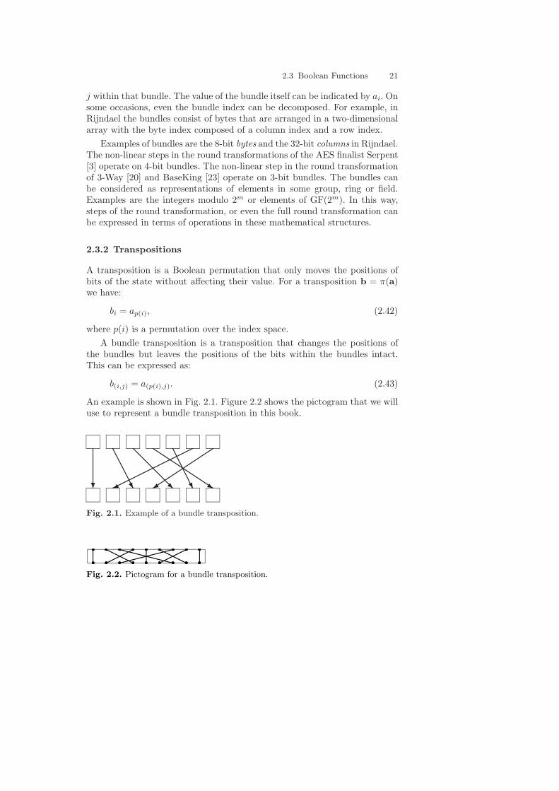
2.3.2 Transpositions

A transposition is a Boolean permutation that only moves the positions ofbits of the state without affecting their value. For a transposition b = π(a)we have:

bi = ap(i), (2.42)

where p(i) is a permutation over the index space.A bundle transposition is a transposition that changes the positions of

the bundles but leaves the positions of the bits within the bundles intact.This can be expressed as:

b(i,j) = a(p(i),j). (2.43)

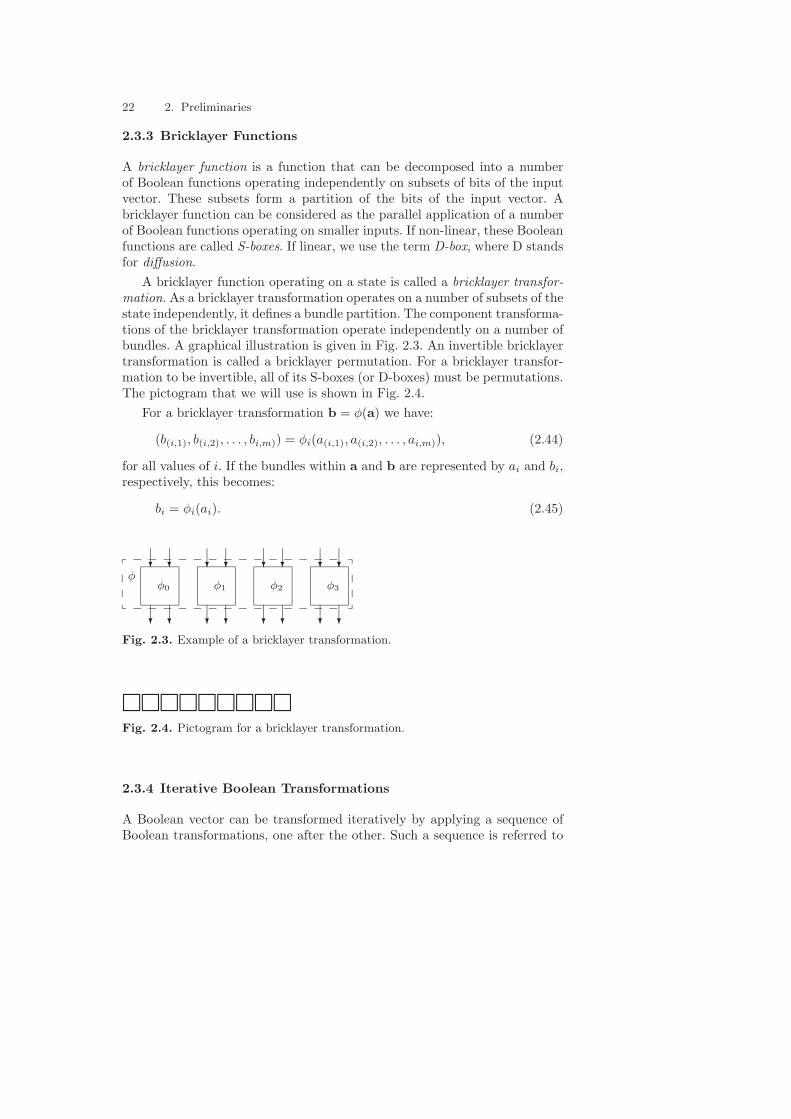
An example is shown in Fig. 2.1. Figure 2.2 shows the pictogram that we willuse to represent a bundle transposition in this book.

� � � ��

Fig. 2.1. Example of a bundle transposition.

Fig. 2.2. Pictogram for a bundle transposition.

22 2. Preliminaries

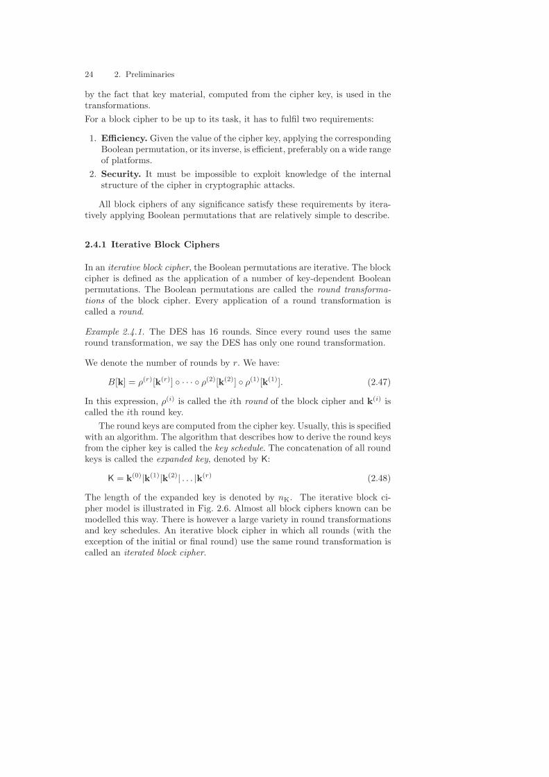
2.3.3 Bricklayer Functions

A bricklayer function is a function that can be decomposed into a numberof Boolean functions operating independently on subsets of bits of the inputvector. These subsets form a partition of the bits of the input vector. Abricklayer function can be considered as the parallel application of a numberof Boolean functions operating on smaller inputs. If non-linear, these Booleanfunctions are called S-boxes. If linear, we use the term D-box, where D standsfor diffusion.

A bricklayer function operating on a state is called a bricklayer transfor-mation. As a bricklayer transformation operates on a number of subsets of thestate independently, it defines a bundle partition. The component transforma-tions of the bricklayer transformation operate independently on a number ofbundles. A graphical illustration is given in Fig. 2.3. An invertible bricklayertransformation is called a bricklayer permutation. For a bricklayer transfor-mation to be invertible, all of its S-boxes (or D-boxes) must be permutations.The pictogram that we will use is shown in Fig. 2.4.

For a bricklayer transformation b = φ(a) we have:

(b(i,1), b(i,2), . . . , bi,m)) = φi(a(i,1), a(i,2), . . . , ai,m)), (2.44)

for all values of i. If the bundles within a and b are represented by ai and bi,respectively, this becomes:

bi = φi(ai). (2.45)

� �

� �

� �

� �

� �

� �

� �

� �

φ0 φ1 φ2 φ3

φ

Fig. 2.3. Example of a bricklayer transformation.

Fig. 2.4. Pictogram for a bricklayer transformation.

2.3.4 Iterative Boolean Transformations

A Boolean vector can be transformed iteratively by applying a sequence ofBoolean transformations, one after the other. Such a sequence is referred to

2.4 Block Ciphers 23

as an iterative Boolean transformation. If the individual Boolean transfor-mations are denoted with ρ(i), an iterative Boolean transformation is of theform:

β = ρ(r) ◦ . . . ◦ ρ(2) ◦ ρ(1). (2.46)

A schematic illustration is given in Fig. 2.5. We have b = β(d), whered = a(0),b = a(m) and a(i) = ρ(i)(a(i−1)). The value of a(i) is called theintermediate state. An iterative Boolean transformation that is a sequence ofBoolean permutations is an iterative Boolean permutation.

ρ(1)

ρ(2)

ρ(3)

�

�

�

�

�

�

�

�

�

�

�

�

�

�

�

�

�

�

�

�

�

�

�

�

�

�

�

�

�

�

�

�

Fig. 2.5. Iterative Boolean transformation.

2.4 Block Ciphers

A block cipher transforms plaintext blocks of a fixed length nb to ciphertextblocks of the same length under the influence of a cipher key k. More precisely,a block cipher is a set of Boolean permutations operating on nb-bit vectors.This set contains a Boolean permutation for each value of the cipher key k. Inthis book we only consider block ciphers in which the cipher key is a Booleanvector. If the number of bits in the cipher key is denoted by nk, a block cipherconsists of 2nk Boolean permutations.

The operation of transforming a plaintext block into a ciphertext block iscalled encryption, and the operation of transforming a ciphertext block intoa plaintext block is called decryption.

Usually, block ciphers are specified by an encryption algorithm, beingthe sequence of transformations to be applied to the plaintext to obtainthe ciphertext. These transformations are operations with a relatively simpledescription. The resulting Boolean permutation depends on the cipher key

24 2. Preliminaries

by the fact that key material, computed from the cipher key, is used in thetransformations.For a block cipher to be up to its task, it has to fulfil two requirements:

1. Efficiency. Given the value of the cipher key, applying the correspondingBoolean permutation, or its inverse, is efficient, preferably on a wide rangeof platforms.

2. Security. It must be impossible to exploit knowledge of the internalstructure of the cipher in cryptographic attacks.

All block ciphers of any significance satisfy these requirements by itera-tively applying Boolean permutations that are relatively simple to describe.

2.4.1 Iterative Block Ciphers

In an iterative block cipher, the Boolean permutations are iterative. The blockcipher is defined as the application of a number of key-dependent Booleanpermutations. The Boolean permutations are called the round transforma-tions of the block cipher. Every application of a round transformation iscalled a round.

Example 2.4.1. The DES has 16 rounds. Since every round uses the sameround transformation, we say the DES has only one round transformation.

We denote the number of rounds by r. We have:

B[k] = ρ(r)[k(r)] ◦ · · · ◦ ρ(2)[k(2)] ◦ ρ(1)[k(1)]. (2.47)

In this expression, ρ(i) is called the ith round of the block cipher and k(i) iscalled the ith round key.

The round keys are computed from the cipher key. Usually, this is specifiedwith an algorithm. The algorithm that describes how to derive the round keysfrom the cipher key is called the key schedule. The concatenation of all roundkeys is called the expanded key, denoted by K:

K = k(0)|k(1)|k(2)| . . . |k(r) (2.48)

The length of the expanded key is denoted by nK. The iterative block ci-pher model is illustrated in Fig. 2.6. Almost all block ciphers known can bemodelled this way. There is however a large variety in round transformationsand key schedules. An iterative block cipher in which all rounds (with theexception of the initial or final round) use the same round transformation iscalled an iterated block cipher.

2.4 Block Ciphers 25

�k(3)

�k(2)

�k(1)

�k

ρ(1)

ρ(2)

ρ(3)

�

�

�

�

�

�

�

�

�

�

�

�

�

�

�

�

�

�

�

�

�

�

�

�

�

�

�

�

�

�

�

�

Fig. 2.6. Iterative block cipher with three rounds.

2.4.2 Key-Alternating Block Ciphers

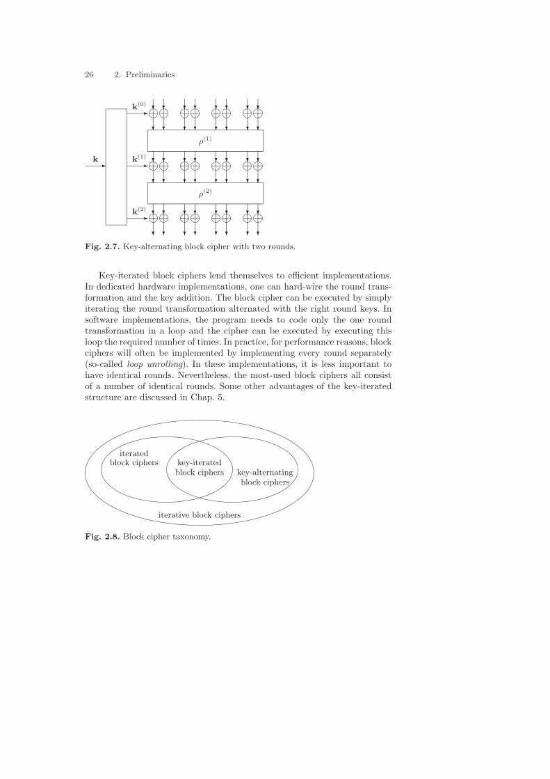
Rijndael belongs to a class of block ciphers in which the round key is ap-plied in a particularly simple way: the key-alternating block ciphers. A key-alternating block cipher is an iterative block cipher with the following prop-erties:

1. Alternation. The cipher is defined as the alternated application of key-independent round transformations and key additions. The first roundkey is added before the first round and the last round key is added afterthe last round.

2. Simple key addition. The round keys are added to the state by meansof a simple XOR A key addition is denoted by σ[k].

We have:

B[k] = σ[k(r)] ◦ ρ(r) ◦ σ[k(r−1)] ◦ · · · ◦ σ[k(1)] ◦ ρ(1) ◦ σ[k(0)]. (2.49)

A graphical illustration is given in Fig. 2.7.Key-alternating block ciphers are a class of block ciphers that lend them-

selves to analysis with respect to the resistance against cryptanalysis. Thiswill become clear in Chaps. 7–9. A special class of key-alternating block ci-phers are the key-iterated block ciphers. In this class, all rounds (except maybethe first or the last) of the cipher use the same round transformation. Wehave:

B[k] = σ[k(r)] ◦ ρ ◦ σ[k(r−1)] ◦ · · · ◦ σ[k(1)] ◦ ρ ◦ σ[k(0)]. (2.50)

In this case, ρ is called the round transformation of the block cipher. Therelations between the different classes of block ciphers that we define hereare shown in Fig. 2.8.

26 2. Preliminaries

�k(2)

�k(1)

�k(0)

k�

ρ(1)

ρ(2)

�

�

�

�

�

�

�

�

�

�

�

�

�

�

�

�

�

�

�

�

�

�

�

�

�

�

�

�

�

�

�

�

�

�

�

�

�

�

�

�

�

�

�

�

�

�

�

�

Fig. 2.7. Key-alternating block cipher with two rounds.

Key-iterated block ciphers lend themselves to efficient implementations.In dedicated hardware implementations, one can hard-wire the round trans-formation and the key addition. The block cipher can be executed by simplyiterating the round transformation alternated with the right round keys. Insoftware implementations, the program needs to code only the one roundtransformation in a loop and the cipher can be executed by executing thisloop the required number of times. In practice, for performance reasons, blockciphers will often be implemented by implementing every round separately(so-called loop unrolling). In these implementations, it is less important tohave identical rounds. Nevertheless, the most-used block ciphers all consistof a number of identical rounds. Some other advantages of the key-iteratedstructure are discussed in Chap. 5.

key-iteratedblock ciphers

iteratedblock ciphers

key-alternatingblock ciphers

iterative block ciphers

Fig. 2.8. Block cipher taxonomy.

2.5 Block Cipher Modes of Operation 27

2.5 Block Cipher Modes of Operation

A block cipher is a very simple cryptographic primitive that can convert aplaintext block to a ciphertext block and vice versa under a given cipherkey. In order to use a cipher to protect the confidentiality or integrity of longmessages, it must be specified how the cipher is used. These specifications arethe so-called modes of operation of a block cipher. In the following sections,we give an overview of the most-widely applied mode of operation. Modes ofencryption are standardized in [43], the use of a block cipher for protectingdata integrity is standardized in [42] and cryptographic hashing based on ablock cipher is standardized in [44].

2.5.1 Block Encryption Modes

In the block encryption modes, the block cipher is used to transform plaintextblocks into ciphertext blocks and vice versa. The message must be split upinto blocks that fit the block length of the cipher. The message can then beencrypted by applying the block cipher to all the blocks independently. Theresulting cryptogram can be decrypted by applying the inverse of the blockcipher to all the blocks independently. This is called the Electronic CodeBook mode (ECB).

A disadvantage of the ECB mode is that if the message has two blocks withthe same value, so will the cryptogram. For this reason another mode has beenproposed: the Cipher Block Chaining (CBC) mode. In this mode, the messageblocks are randomised before applying the block cipher by performing anXOR with the ciphertext block corresponding with the previous messageblock. In CBC decryption, a message block is obtained by applying the inverseblock cipher followed by an XOR with the previous cryptogram block.

Both ECB and CBC modes have the disadvantage that the length of themessage must be an integer multiple of the block length. If this is not thecase, the last block must be padded, i.e. bits must be appended so that ithas the required length. This padding causes the cryptogram to be longerthan the message itself, which may be a disadvantage is some applications.For messages that are larger than one block, padding may be avoided bythe application of so-called ciphertext stealing [70, p. 81], that adds somecomplexity to the treatment of the last message blocks.

2.5.2 Key-Stream Generation Modes

In so-called key-stream generation modes, the cipher is used to generate a key-stream that is used for encryption by means of bitwise XOR with a messagestream. Decryption corresponds with subtracting (XOR) the key-stream bitsfrom the message. Hence, for correct decryption it suffices to generate the

28 2. Preliminaries

same key-stream at both ends. It follows that at both ends the same functioncan be used for the generation of the key-stream and that the inverse cipher isnot required to perform decryption. The feedback modes have the additionaladvantage that there is no need for padding the message and hence that thecryptogram has the same length as the message itself.

In Output Feed Back mode (OFB) and Counter mode, the block cipher isjust used as a synchronous key-stream sequence generator. In OFB mode, thekey-stream generator is a finite state machine in which the state has the blocklength of the cipher and the state updating function consists of encryptionwith the block cipher for some secret value of the key. In Counter mode,the key-stream is the result of applying ECB encryption to a predictablesequence, e.g. an incrementing counter.

In Cipher Feed Back mode (CFB), the key-stream is a key-dependentfunction of the last nb bits of the ciphertext. This function consists of en-cryption with the block cipher for some secret value of the key. Among thekey-stream generation modes, the CFB mode has the advantage that decryp-tion is correct from the moment that the last nb bits of the cryptogram havebeen correctly received. In other words, it has a self-synchronizing property.In the OFB and Counter modes, synchronization must be assured by externalmeans. For a more thorough treatment of block cipher modes of operationfor encryption, we refer to [68, Sect. 7.2.2].

2.5.3 Message Authentication Modes

Many applications do not require the protection of confidentiality of mes-sages but rather the protection of their integrity. As encryption by itself doesnot provide message integrity, a dedicated algorithm must be used. For thispurpose often a cryptographic checksum, requiring a secret key, is computedon a message. Such a cryptographic checksum is called a Message Authenti-cation Code (MAC). In general, the MAC is sent along with the message forthe receiving entity to verify that the message has not been modified alongthe way.

A MAC algorithm can be based on a block cipher. The most widespreadway of using a block cipher as a MAC is called the CBC-MAC. in its simplestform it consists of applying a block cipher in CBC mode on a message andtaking (part) of the last cryptogram block as the MAC. The generation ofa MAC and its verification are very similar processes. The verification con-sists of reconstructing the MAC from the message using the secret key andcomparing it with the MAC received. Hence, similar to the key-stream gen-eration modes of encryption, the CBC-MAC mode of a block cipher does notrequire decryption with the cipher. For a more thorough treatment of messageauthentication codes using a block cipher, we refer to [68, Sect. 9.5.1].

2.6 Conclusions 29

2.5.4 Cryptographic Hashing

In some applications, integrity of a message is obtained in two phases: firstthe message, that may have any length, is compressed to a short, fixed-length message digest with a so-called cryptographic hash function, and sub-sequently the message digest is authenticated. For some applications thishash function must guarantee that it is infeasible to find two messages thathash to the same message digest (collision resistant). For other applications,it suffices that given a message, no other message can be found so that bothhash to the same message digest (second-preimage resistant). For yet otherapplications it suffices that given a message digest, no message can be foundthat hashes to that value (one-way or preimage resistant).

A block cipher can be used as the compression function of an iterated hashfunction by adopting the Davies-Meyer, Matyas-Meyer-Oseas or Miyaguchi-Preneel mode (see [68]). In these modes the length of the hash result (andalso the chaining variable) is the block length. In the assumption that theunderlying block cipher has no weaknesses, and with the current state ofcryptanalysis and technology, a block length of 128 bits is considered sufficientto provide both variants of preimage resistance. If collision resistance is thegoal, we advise the adoption of a block length of 256 bits. For a more thoroughtreatment of cryptographic hashing using a block cipher, we refer to [68,Sect. 9.4.1].

2.6 Conclusions

In this chapter we have given a number of definitions and an introduction tomathematical concepts that are used throughout the book.

3. Specification of Rijndael

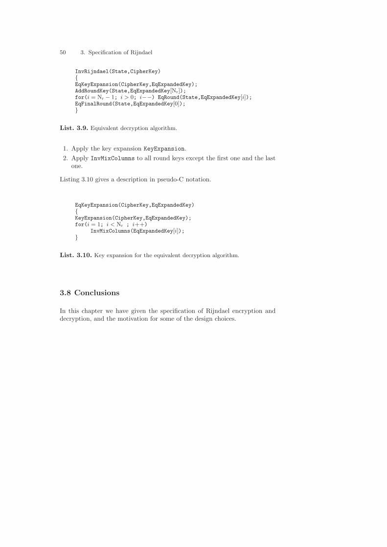
In this chapter we specify the cipher structure and the building blocks ofRijndael. After explaining the difference between the Rijndael specificationsand the AES standard, we specify the external interface to the ciphers. This isfollowed by the description of the Rijndael structure and the steps of its roundtransformation. Subsequently, we specify the number of rounds as a functionof the block and key length, and describe the key schedule. We conclude thischapter with a treatment of algorithms for implementing decryption withRijndael. This chapter is not intended as an implementation guideline. Forimplementation aspects, we refer to Chap. 4.

3.1 Differences between Rijndael and the AES

The only difference between Rijndael and the AES is the range of supportedvalues for the block length and cipher key length.

Rijndael is a block cipher with both a variable block length and a variablekey length. The block length and the key length can be independently spec-ified to any multiple of 32 bits, with a minimum of 128 bits and a maximumof 256 bits. It would be possible to define versions of Rijndael with a higherblock length or key length, but currently there seems no need for it.

The AES fixes the block length to 128 bits, and supports key lengths of128, 192 or 256 bits only. The extra block and key lengths in Rijndael werenot evaluated in the AES selection process, and consequently they are notadopted in the current FIPS standard.

3.2 Input and Output for Encryption and Decryption

The input and output of Rijndael are considered to be one-dimensional arraysof 8-bit bytes. For encryption the input is a plaintext block and a key, and theoutput is a ciphertext block. For decryption, the input is a ciphertext blockand a key, and the output is a plaintext block. The round transformation ofRijndael, and its steps, operate on an intermediate result, called the state.

32 3. Specification of Rijndael

The state can be pictured as a rectangular array of bytes, with four rows.The number of columns in the state is denoted by Nb and is equal to theblock length divided by 32. Let the plaintext block be denoted by

p0p1p2p3 . . . p4·Nb−1,

where p0 denotes the first byte,and p4·Nb−1 denotes the last byte of the plain-text block. Similarly, a ciphertext block can be denoted by

c0c1c2c3 . . . c4·Nb−1.

Let the state be denoted by

ai,j , 0 ≤ i < 4, 0 ≤ j < Nb.

where ai,j denotes the byte in row i and column j. The input bytes aremapped onto the state bytes in the order a0,0, a1,0, a2,0, a3,0, a0,1, a1,1, a2,1,a3,1, . . . . For encryption, the input is a plaintext block and the mapping is

ai,j = pi+4j , 0 ≤ i < 4, 0 ≤ j < Nb. (3.1)

For decryption, the input is a ciphertext block and the mapping is

ai,j = ci+4j , 0 ≤ i < 4, 0 ≤ j < Nb. (3.2)

At the end of the encryption, the ciphertext is extracted from the state bytaking the state bytes in the same order:

ci = ai mod 4,i/4, 0 ≤ i < 4Nb. (3.3)

At the end of decryption, the plaintext block is extracted from the stateaccording to

pi = ai mod 4,i/4, 0 ≤ i < 4Nb. (3.4)

Similarly, the key is mapped onto a two-dimensional cipher key. The cipherkey is pictured as a rectangular array with four rows similar to the state. Thenumber of columns of the cipher key is denoted by Nk and is equal to thekey length divided by 32. The bytes of the key are mapped onto the bytes ofthe cipher key in the order: k0,0, k1,0, k2,0, k3,0, k0,1, k1,1, k2,1, k3,1, k4,1 . . . .If we denote the key by:

z0z1z2z3 . . . z4·Nk−1,

then

ki,j = zi+4j , 0 ≤ i < 4, 0 ≤ j < Nk. (3.5)

The representation of the state and cipher key and the mappings plaintext–state and key–cipher key are illustrated in Fig. 3.1.

3.3 Structure of Rijndael 33

k0

k1

k2

k3

k4

k5

k6

k7

k8

k9

k10

k11

k12

k13

k14

k15

k16

k17

k18

k19

k20

k21

k22

k23

p0

p1

p2

p3

p4

p5

p6

p7

p8

p9

p10

p11

p12

p13

p14

p15

Fig. 3.1. State and cipher key layout for the case Nb = 4 and Nk = 6.

3.3 Structure of Rijndael

Rijndael is a key-iterated block cipher: it consists of the repeated applicationof a round transformation on the state. The number of rounds is denoted byNr and depends on the block length and the key length.

Note that in this chapter, contrary to the definitions (2.47)–(2.50), thekey addition is included in the round transformation. This is done in orderto make the description in this chapter consistent with the description in theFIPS standard.

Following a suggestion of B. Gladman, we changed the names of somesteps with respect to the description given in our original AES submission.The new names are more consistent, and are also adopted in the FIPS stan-dard. We made some further changes, all in order to make the descriptionmore clear and complete. No changes have been made to the block cipheritself.

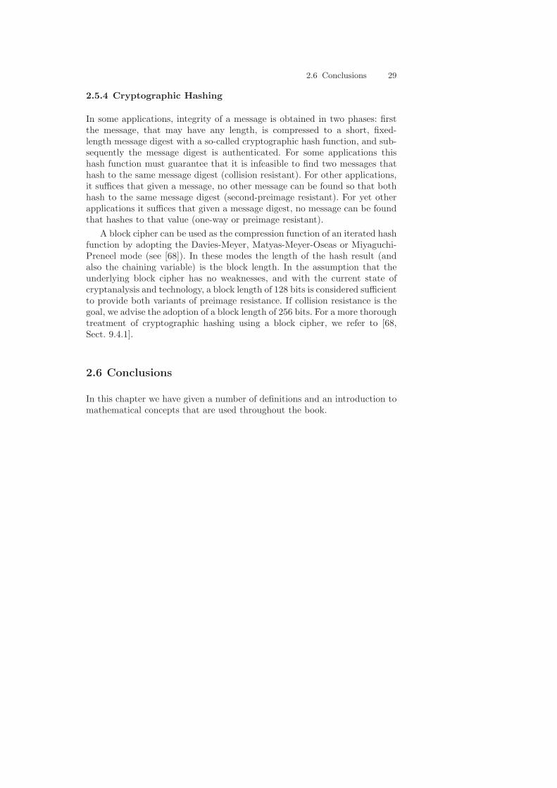
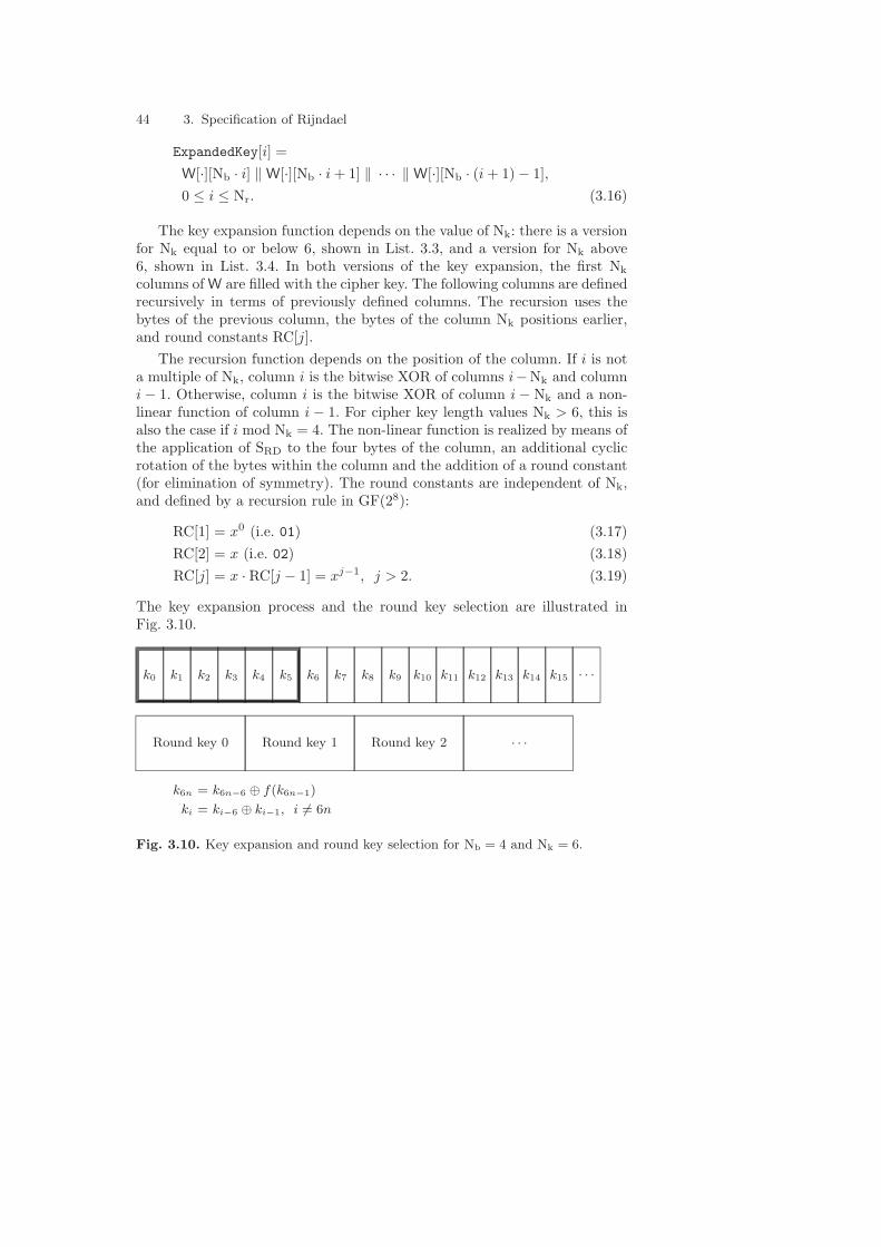
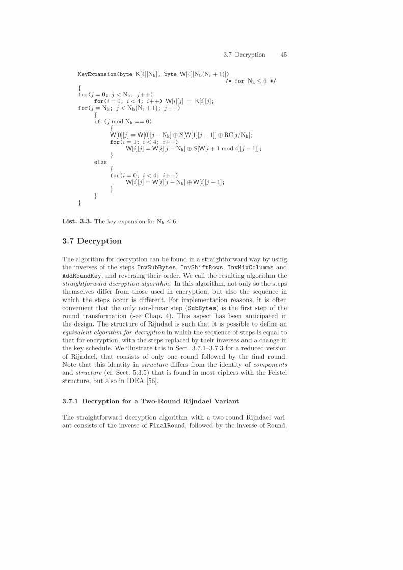
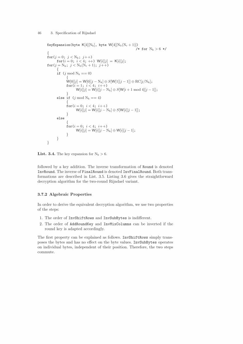
An encryption with Rijndael consists of an initial key addition, denotedby AddRoundKey, followed by Nr−1 applications of the transformation Round,and finally one application of FinalRound. The initial key addition and everyround take as input the State and a round key. The round key for round iis denoted by ExpandedKey[i], and ExpandedKey[0] denotes the input of theinitial key addition. The derivation of ExpandedKey from the CipherKey isdenoted by KeyExpansion. A high-level description of Rijndael in pseudo-Cnotation is shown in List. 3.1.

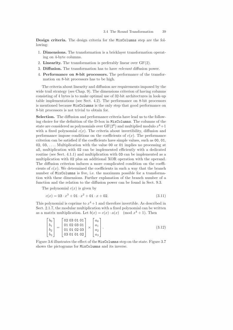
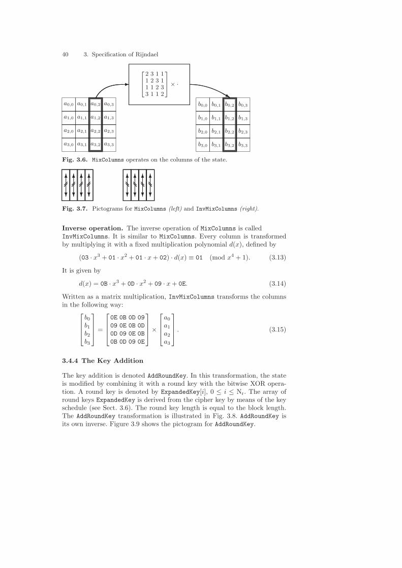
3.4 The Round Transformation

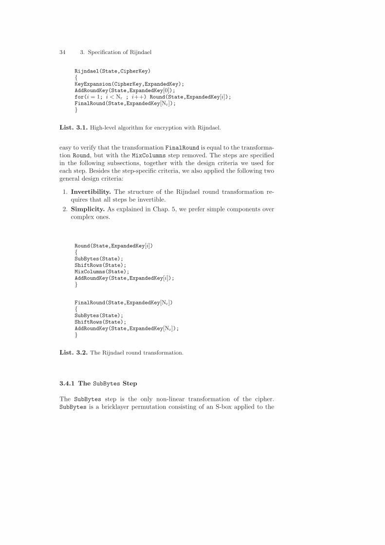
The round transformation is denoted Round, and is a sequence of four trans-formations, called steps. This is shown in List. 3.2. The final round of the ci-pher is slightly different. It is denoted FinalRound and also shown in List. 3.2.In the listings, the transformations (Round, SubBytes, ShiftRows, . . . ) op-erate on arrays to which pointers (State, ExpandedKey[i]) are provided. It is


Rijndael(State,CipherKey){KeyExpansion(CipherKey,ExpandedKey);AddRoundKey(State,ExpandedKey[0]);for(i = 1; i < Nr ; i++) Round(State,ExpandedKey[i]);FinalRound(State,ExpandedKey[Nr]);}

List. 3.1. High-level algorithm for encryption with Rijndael.

easy to verify that the transformation FinalRound is equal to the transforma-tion Round, but with the MixColumns step removed. The steps are specifiedin the following subsections, together with the design criteria we used foreach step. Besides the step-specific criteria, we also applied the following twogeneral design criteria:

1. Invertibility. The structure of the Rijndael round transformation re-quires that all steps be invertible.

2. Simplicity. As explained in Chap. 5, we prefer simple components overcomplex ones.

Round(State,ExpandedKey[i]){SubBytes(State);ShiftRows(State);MixColumns(State);AddRoundKey(State,ExpandedKey[i]);}

FinalRound(State,ExpandedKey[Nr]){SubBytes(State);ShiftRows(State);AddRoundKey(State,ExpandedKey[Nr]);}

List. 3.2. The Rijndael round transformation.

3.4.1 The SubBytes Step

The SubBytes step is the only non-linear transformation of the cipher.SubBytes is a bricklayer permutation consisting of an S-box applied to the

3.4 The Round Transformation 35

bytes of the state. We denote the particular S-box being used in Rijndaelby SRD. Figure 3.2 illustrates the effect of the SubBytes step on the state.Figure 3.3 shows the pictograms that we will use to represent SubBytes andits inverse.

a0,0

a1,0

a2,0

a3,0

a0,1

a1,1

a2,1

a3,1

a0,2

a1,2

a2,2

a3,2

a0,3

a1,3

a2,3

a3,3

b0,0

b1,0

b2,0

b3,0

b0,1

b1,1

b2,1

b3,1

b0,2

b1,2

b2,2

b3,2

b0,3

b1,3

b2,3

b3,3

SRD�

�

Fig. 3.2. SubBytes acts on the individual bytes of the state.

�

�

�

�

�

�

�

�

�

�

�

�

�

�

�

�

�

�

�

�

�

�

�

�

�

�

�

�

�

�

�

�

Fig. 3.3. The pictograms for SubBytes (left) and InvSubBytes (right).

Design criteria for SRD. We have applied the following design criteria forSRD, appearing in order of importance:

1. Non-linearity.a) Correlation. The maximum input-output correlation amplitude

must be as small as possible.b) Difference propagation probability. The maximum difference

propagation probability must be as small as possible.2. Algebraic complexity. The algebraic expression of SRD in GF(28) has

to be complex.

Only one S-box is used for all byte positions. This is certainly not a necessity:SubBytes could as easily be defined with different S-boxes for every byte. Thisissue is discussed in Chap. 5. The non-linearity criteria are inspired by linearand differential cryptanalysis. Chap. 9 discusses this in depth.

Selection of SRD. In [74], K. Nyberg gives several construction methods forS-boxes with good non-linearity. For invertible S-boxes operating on bytes,


the maximum correlation amplitude can be made as low as 2−3, and the max-imum difference propagation probability can be as low as 2−6. We decided tochoose — from the alternatives described in [74] — the S-box that is definedby the following function in GF(28):

g : a → b = a−1. (3.6)

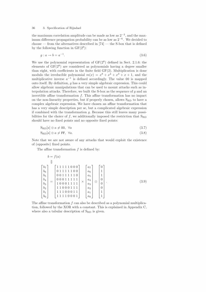
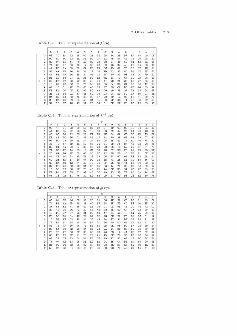
We use the polynomial representation of GF(28) defined in Sect. 2.1.6: theelements of GF(28) are considered as polynomials having a degree smallerthan eight, with coefficients in the finite field GF(2). Multiplication is donemodulo the irreducible polynomial m(x) = x8 + x4 + x3 + x + 1, and themultiplicative inverse a−1 is defined accordingly. The value 00 is mappedonto itself. By definition, g has a very simple algebraic expression. This couldallow algebraic manipulations that can be used to mount attacks such as in-terpolation attacks. Therefore, we built the S-box as the sequence of g and aninvertible affine transformation f . This affine transformation has no impacton the non-linearity properties, but if properly chosen, allows SRD to have acomplex algebraic expression. We have chosen an affine transformation thathas a very simple description per se, but a complicated algebraic expressionif combined with the transformation g. Because this still leaves many possi-bilities for the choice of f , we additionally imposed the restriction that SRD

should have no fixed points and no opposite fixed points:

SRD[a] ⊕ a = 00, ∀a (3.7)SRD[a] ⊕ a = FF, ∀a. (3.8)

Note that we are not aware of any attacks that would exploit the existenceof (opposite) fixed points.

The affine transformation f is defined by:

b = f(a)�

b7

b6

b5

b4

b3

b2

b1

b0

=

1 1 1 1 1 0 0 00 1 1 1 1 1 0 00 0 1 1 1 1 1 00 0 0 1 1 1 1 11 0 0 0 1 1 1 11 1 0 0 0 1 1 11 1 1 0 0 0 1 11 1 1 1 0 0 0 1

×

a7

a6

a5

a4

a3

a2

a1

a0

⊕

01100011

. (3.9)

The affine transformation f can also be described as a polynomial multiplica-tion, followed by the XOR with a constant. This is explained in Appendix C,where also a tabular description of SRD is given.


Inverse operation. The inverse operation of SubBytes is calledInvSubBytes. It is a bricklayer permutation consisting of the inverse S-boxSRD

−1 applied to the bytes of the state. The inverse S-box SRD−1 is obtained

by applying the inverse of the affine transformation (3.9) followed by takingthe multiplicative inverse in GF(28). The inverse of (3.9) is specified by:

x7

x6

x5

x4

x3

x2

x1

x0

=

0 1 0 1 0 0 1 00 0 1 0 1 0 0 11 0 0 1 0 1 0 00 1 0 0 1 0 1 00 0 1 0 0 1 0 11 0 0 1 0 0 1 00 1 0 0 1 0 0 11 0 1 0 0 1 0 0

×

y7

y6

y5

y4

y3

y2

y1

y0

⊕

00000101

. (3.10)

Tabular descriptions of SRD−1 and f−1 are given in Appendix C.

3.4.2 The ShiftRows Step

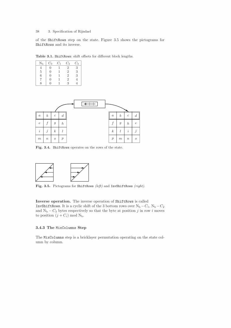
The ShiftRows step is a byte transposition that cyclically shifts the rows ofthe state over different offsets. Row 0 is shifted over C0 bytes, row 1 overC1 bytes, row 2 over C2 bytes and row 3 over C3 bytes, so that the byte atposition j in row i moves to position (j − Ci) mod Nb. The shift offsets C0,C1, C2 and C3 depend on the value of Nb.

Design criteria for the offsets. The design criteria for the offsets are thefollowing:

1. Diffusion optimal. The four offsets have to be different (see Defini-tion 9.4.1).

2. Other diffusion effects. The resistance against truncated differentialattacks (see Chap. 10) and saturation attacks has to be maximized.

Diffusion optimality is important in providing resistance against differentialand linear cryptanalysis. The other diffusion effects are only relevant whenthe block length is larger than 128 bits.

Selection of the offsets. The simplicity criterion dictates that one offset istaken equal to 0. In fact, for a block length of 128 bits, the offsets have to be0, 1, 2 and 3. The assignment of offsets to rows is arbitrary. For block lengthslarger than 128 bit, there are more possibilities. Detailed studies of truncateddifferential attacks and saturation attacks on reduced versions of Rijndaelshow that not all choices are equivalent. For certain choices, the attacks canbe extended with one round. Among the choices that are best with respectto saturation and truncated differential attacks, we picked the simplest ones.The different values are specified in Table 3.1. Figure 3.4 illustrates the effect


of the ShiftRows step on the state. Figure 3.5 shows the pictograms forShiftRows and its inverse.

Table 3.1. ShiftRows: shift offsets for different block lengths.

Nb C0 C1 C2 C3

4 0 1 2 35 0 1 2 36 0 1 2 37 0 1 2 48 0 1 3 4

a

e

i

m

b

f

j

n

c

g

k

o

d

h

l

p

a

f

k

p

b

g

l

m

c

h

i

n

d

e

j

o

��

Fig. 3.4. ShiftRows operates on the rows of the state.

��

�

��

�

Fig. 3.5. Pictograms for ShiftRows (left) and InvShiftRows (right).

Inverse operation. The inverse operation of ShiftRows is calledInvShiftRows. It is a cyclic shift of the 3 bottom rows over Nb−C1, Nb−C2

and Nb −C3 bytes respectively so that the byte at position j in row i movesto position (j + Ci) mod Nb.

3.4.3 The MixColumns Step

The MixColumns step is a bricklayer permutation operating on the state col-umn by column.


Design criteria. The design criteria for the MixColumns step are the fol-lowing:

1. Dimensions. The transformation is a bricklayer transformation operat-ing on 4-byte columns.

2. Linearity. The transformation is preferably linear over GF(2).3. Diffusion. The transformation has to have relevant diffusion power.4. Performance on 8-bit processors. The performance of the transfor-

mation on 8-bit processors has to be high.

The criteria about linearity and diffusion are requirements imposed by thewide trail strategy (see Chap. 9). The dimensions criterion of having columnsconsisting of 4 bytes is to make optimal use of 32-bit architectures in look-uptable implementations (see Sect. 4.2). The performance on 8-bit processorsis mentioned because MixColumns is the only step that good performance on8-bit processors is not trivial to obtain for.

Selection. The diffusion and performance criteria have lead us to the follow-ing choice for the definition of the D-box in MixColumns. The columns of thestate are considered as polynomials over GF(28) and multiplied modulo x4+1with a fixed polynomial c(x). The criteria about invertibility, diffusion andperformance impose conditions on the coefficients of c(x). The performancecriterion can be satisfied if the coefficients have simple values, such as 00, 01,02, 03, . . . . Multiplication with the value 00 or 01 implies no processing atall, multiplication with 02 can be implemented efficiently with a dedicatedroutine (see Sect. 4.1.1) and multiplication with 03 can be implemented as amultiplication with 02 plus an additional XOR operation with the operand.The diffusion criterion induces a more complicated condition on the coeffi-cients of c(x). We determined the coefficients in such a way that the branchnumber of MixColumns is five, i.e. the maximum possible for a transforma-tion with these dimensions. Further explanation of the branch number of afunction and the relation to the diffusion power can be found in Sect. 9.3.

The polynomial c(x) is given by

c(x) = 03 · x3 + 01 · x2 + 01 · x + 02. (3.11)

This polynomial is coprime to x4 +1 and therefore invertible. As described inSect. 2.1.7, the modular multiplication with a fixed polynomial can be writtenas a matrix multiplication. Let b(x) = c(x) · a(x) (mod x4 + 1). Then

b0

b1

b2

b3

=

02 03 01 0101 02 03 0101 01 02 0303 01 01 02

×

a0

a1

a2

a3

. (3.12)

Figure 3.6 illustrates the effect of the MixColumns step on the state. Figure 3.7shows the pictograms for MixColumns and its inverse.


a0,0

a1,0

a2,0

a3,0

a0,1

a1,1

a2,1

a3,1

a0,2

a1,2

a2,2

a3,2

a0,3

a1,3

a2,3

a3,3

b0,0

b1,0

b2,0

b3,0

b0,1

b1,1

b2,1

b3,1

b0,2

b1,2

b2,2

b3,2

b0,3

b1,3

b2,3

b3,3

2 3 1 11 2 3 11 1 2 33 1 1 2

× ·�

Fig. 3.6. MixColumns operates on the columns of the state.

�

�

�

�

�

�

�

�

Fig. 3.7. Pictograms for MixColumns (left) and InvMixColumns (right).

Inverse operation. The inverse operation of MixColumns is calledInvMixColumns. It is similar to MixColumns. Every column is transformedby multiplying it with a fixed multiplication polynomial d(x), defined by

(03 · x3 + 01 · x2 + 01 · x + 02) · d(x) ≡ 01 (mod x4 + 1). (3.13)

It is given by

d(x) = 0B · x3 + 0D · x2 + 09 · x + 0E. (3.14)

Written as a matrix multiplication, InvMixColumns transforms the columnsin the following way:

b0

b1

b2

b3

=

0E 0B 0D 0909 0E 0B 0D0D 09 0E 0B0B 0D 09 0E

×

a0

a1

a2

a3

. (3.15)

3.4.4 The Key Addition

The key addition is denoted AddRoundKey. In this transformation, the stateis modified by combining it with a round key with the bitwise XOR opera-tion. A round key is denoted by ExpandedKey[i], 0 ≤ i ≤ Nr. The array ofround keys ExpandedKey is derived from the cipher key by means of the keyschedule (see Sect. 3.6). The round key length is equal to the block length.The AddRoundKey transformation is illustrated in Fig. 3.8. AddRoundKey isits own inverse. Figure 3.9 shows the pictogram for AddRoundKey.

3.5 The Number of Rounds 41

a0,0

a1,0

a2,0

a3,0

a0,1

a1,1

a2,1

a3,1

a0,2

a1,2

a2,2

a3,2

a0,3

a1,3

a2,3

a3,3

⊕

k0,0

k1,0

k2,0

k3,0

k0,1

k1,1

k2,1

k3,1

k0,2

k1,2

k2,2

k3,2

k0,3

k1,3

k2,3

k3,3

=

b0,0

b1,0

b2,0

b3,0

b0,1

b1,1

b2,1

b3,1

b0,2

b1,2

b2,2

b3,2

b0,3

b1,3

b2,3

b3,3

Fig. 3.8. In AddRoundKey, the round key is added to the state with a bitwise XOR.

Fig. 3.9. Pictogram for AddRoundKey.

3.5 The Number of Rounds

The current state-of-the-art in cryptanalysis indicates that the resistanceof iterative block ciphers against cryptanalytic attacks increases with thenumber of rounds.

We have determined the number of rounds by considering the maximumnumber of rounds for which shortcut attacks (see Sect. 5.5.1) have been foundthat are significantly more efficient than an exhaustive key search. Subse-quently, we added a considerable security margin. For Rijndael with a blocklength and key length of 128 bits, no shortcut attacks had been found for re-duced versions with more than six rounds. We added four rounds as a securitymargin. This is a conservative approach, because:

1. Two rounds of Rijndael provide ‘full diffusion’ in the following sense:every state bit depends on all state bits two rounds ago, or a change inone state bit is likely to affect half of the state bits after two rounds.Adding four rounds can be seen as adding a ‘full diffusion step’ at thebeginning and at the end of the cipher. The high diffusion of the Rijndaelround transformation is thanks to its uniform structure that operates onall state bits. For so-called Feistel ciphers, a round only operates on halfof the state bits and full diffusion can at best be obtained after threerounds and in practice it typically takes four rounds or more.

2. Generally, linear cryptanalysis, differential cryptanalysis and truncateddifferential attacks exploit a propagation trail through n rounds in orderto attack n + 1 or n + 2 rounds. This is also the case for the saturationattack (see Sect. 10.2) that uses a four-round propagation structure to


attack six rounds. In this respect, adding four rounds actually doublesthe number of rounds through which a propagation trail has to be found.

For Rijndael versions with a longer key, the number of rounds was raisedby one for every additional 32 bits in the cipher key. This was done for thefollowing reasons:

1. One of the main objectives is the absence of shortcut attacks, i.e. attacksthat are more efficient than an exhaustive key search. Since the workloadof an exhaustive key search grows with the key length, shortcut attackscan afford to be less efficient for longer keys.

2. (Partially) known-key and related-key attacks exploit the knowledge ofcipher key bits or the ability to apply different cipher keys. If the ci-pher key grows, the range of possibilities available to the cryptanalystincreases.

The publications on the security of Rijndael with longer keys have shown thatthis strategy leads to an adequate security margin [31, 36, 62]. For Rijndaelversions with a higher block length, the number of rounds is raised by onefor every additional 32 bits in the block length, for the following reasons:

1. For a block length above 128 bits, it takes three rounds to realize that fulldiffusion, i.e. the diffusion power of the round transformation, relative tothe block length, diminishes with the block length.

2. The larger block length causes the range of possible patterns that canbe applied at the input/output of a sequence of rounds to increase. Thisadditional flexibility may allow the extension of attacks by one or morerounds.

We have found that extensions of attacks by a single round are even hardto realize for the maximum block length of 256 bits. Therefore, this is aconservative margin.

Table 3.2 lists the value of Nr as a function of Nb and Nk. For the AES,Nb is fixed to the value 4; Nr = 10 for 128-bit keys (Nk = 4), Nr = 12 for192-bit keys (Nk = 6) and Nr = 14 for 256-bit keys (Nk = 8).

Table 3.2. Number of rounds (Nr) as a function of Nb (Nb = block length/32) andNk (key length/32).

Nb

Nk 4 5 6 7 8

4 10 11 12 13 145 11 11 12 13 146 12 12 12 13 147 13 13 13 13 148 14 14 14 14 14

3.6 Key Schedule 43

3.6 Key Schedule

The key schedule consists of two components: the key expansion and theround key selection. The key expansion specifies how ExpandedKey is derivedfrom the cipher key. The total number of bits in ExpandedKey is equal tothe block length multiplied by the number of rounds plus 1, since the cipherrequires one round key for the initial key addition, and one for each of therounds. Please note that the ExpandedKey is always derived from the cipherkey; it should never be specified directly.

3.6.1 Design Criteria

The key expansion has been chosen according to the following criteria:

1. Efficiency.a) Working memory. It should be possible to execute the key schedule

using a small amount of working memory.b) Performance. It should have a high performance on a wide range

of processors.2. Symmetry elimination. It should use round constants to eliminate

symmetries.3. Diffusion. It should have an efficient diffusion of cipher key differences

into the expanded key,4. Non-linearity. It should exhibit enough non-linearity to prohibit the

full determination of differences in the expanded key from cipher keydifferences only.

For a more thorough treatment of the criteria underlying the design of thekey schedule, we refer to Sect. 5.8.

3.6.2 Selection

In order to be efficient on 8-bit processors, a lightweight, byte-oriented ex-pansion scheme has been adopted. The application of the non-linear SRD

ensures the non-linearity of the scheme, without adding much in the way oftemporary storage requirements on an 8-bit processor.

During the key expansion the cipher key is expanded into an expandedkey array, consisting of 4 rows and Nb(Nr + 1) columns. This array is heredenoted by W[4][Nb(Nr+1)]. The round key of the ith round, ExpandedKey[i],is given by the columns Nb · i to Nb · (i + 1) − 1 of W:


ExpandedKey[i] =W[·][Nb · i] ‖ W[·][Nb · i + 1] ‖ · · · ‖ W[·][Nb · (i + 1) − 1],0 ≤ i ≤ Nr. (3.16)

The key expansion function depends on the value of Nk: there is a versionfor Nk equal to or below 6, shown in List. 3.3, and a version for Nk above6, shown in List. 3.4. In both versions of the key expansion, the first Nk

columns of W are filled with the cipher key. The following columns are definedrecursively in terms of previously defined columns. The recursion uses thebytes of the previous column, the bytes of the column Nk positions earlier,and round constants RC[j].

The recursion function depends on the position of the column. If i is nota multiple of Nk, column i is the bitwise XOR of columns i−Nk and columni − 1. Otherwise, column i is the bitwise XOR of column i − Nk and a non-linear function of column i − 1. For cipher key length values Nk > 6, this isalso the case if i mod Nk = 4. The non-linear function is realized by means ofthe application of SRD to the four bytes of the column, an additional cyclicrotation of the bytes within the column and the addition of a round constant(for elimination of symmetry). The round constants are independent of Nk,and defined by a recursion rule in GF(28):

RC[1] = x0 (i.e. 01) (3.17)RC[2] = x (i.e. 02) (3.18)RC[j] = x · RC[j − 1] = xj−1, j > 2. (3.19)

The key expansion process and the round key selection are illustrated inFig. 3.10.

k0 k1 k2 k3 k4 k5 k6 k7 k8 k9 k10 k11 k12 k13 k14 k15. . .

Round key 0 Round key 1 Round key 2 . . .

k6n = k6n−6 ⊕ f(k6n−1)

ki = ki−6 ⊕ ki−1, i �= 6n

Fig. 3.10. Key expansion and round key selection for Nb = 4 and Nk = 6.

3.7 Decryption 45

KeyExpansion(byte K[4][Nk], byte W[4][Nb(Nr + 1)])/* for Nk ≤ 6 */

{for(j = 0; j < Nk; j++)

for(i = 0; i < 4; i++) W[i][j] = K[i][j];for(j = Nk; j < Nb(Nr + 1); j++)

{if (j mod Nk == 0)

{W[0][j] = W[0][j − Nk] ⊕ S[W[1][j − 1]] ⊕ RC[j/Nk];for(i = 1; i < 4; i++)

W[i][j] = W[i][j − Nk] ⊕ S[W[i + 1 mod 4][j − 1]];}

else{for(i = 0; i < 4; i++)

W[i][j] = W[i][j − Nk] ⊕ W[i][j − 1];}

}}

List. 3.3. The key expansion for Nk ≤ 6.

3.7 Decryption

The algorithm for decryption can be found in a straightforward way by usingthe inverses of the steps InvSubBytes, InvShiftRows, InvMixColumns andAddRoundKey, and reversing their order. We call the resulting algorithm thestraightforward decryption algorithm. In this algorithm, not only so the stepsthemselves differ from those used in encryption, but also the sequence inwhich the steps occur is different. For implementation reasons, it is oftenconvenient that the only non-linear step (SubBytes) is the first step of theround transformation (see Chap. 4). This aspect has been anticipated inthe design. The structure of Rijndael is such that it is possible to define anequivalent algorithm for decryption in which the sequence of steps is equal tothat for encryption, with the steps replaced by their inverses and a change inthe key schedule. We illustrate this in Sect. 3.7.1–3.7.3 for a reduced versionof Rijndael, that consists of only one round followed by the final round.Note that this identity in structure differs from the identity of componentsand structure (cf. Sect. 5.3.5) that is found in most ciphers with the Feistelstructure, but also in IDEA [56].

3.7.1 Decryption for a Two-Round Rijndael Variant

The straightforward decryption algorithm with a two-round Rijndael vari-ant consists of the inverse of FinalRound, followed by the inverse of Round,


KeyExpansion(byte K[4][Nk], byte W[4][Nb(Nr + 1)])/* for Nk > 6 */

{for(j = 0; j < Nk; j++)

for(i = 0; i < 4; ++) W[i][j] = K[i][j];for(j = Nk; j < Nb(Nr + 1); j++)

{if (j mod Nk == 0)

{W[0][j] = W[0][j − Nk] ⊕ S[W[1][j − 1]] ⊕ RC[j/Nk];for(i = 1; i < 4; i++)

W[i][j] = W[i][j − Nk] ⊕ S[W[i + 1 mod 4][j − 1]];}

else if (j mod Nk == 4){for(i = 0; i < 4; i++)

W[i][j] = W[i][j − Nk] ⊕ S[W[i][j − 1]];}

else{for(i = 0; i < 4; i++)

W[i][j] = W[i][j − Nk] ⊕ W[i][j − 1];}

}}

List. 3.4. The key expansion for Nk > 6.

followed by a key addition. The inverse transformation of Round is denotedInvRound. The inverse of FinalRound is denoted InvFinalRound. Both trans-formations are described in List. 3.5. Listing 3.6 gives the straightforwarddecryption algorithm for the two-round Rijndael variant.

3.7.2 Algebraic Properties

In order to derive the equivalent decryption algorithm, we use two propertiesof the steps:

1. The order of InvShiftRows and InvSubBytes is indifferent.2. The order of AddRoundKey and InvMixColumns can be inverted if the

round key is adapted accordingly.

The first property can be explained as follows. InvShiftRows simply trans-poses the bytes and has no effect on the byte values. InvSubBytes operateson individual bytes, independent of their position. Therefore, the two stepscommute.

3.7 Decryption 47

InvRound(State,ExpandedKey[i]){AddRoundKey(State,ExpandedKey[i]);InvMixColumns(State);InvShiftRows(State);InvSubBytes(State);}

InvFinalRound(State,ExpandedKey[Nr]){AddRoundKey(State,ExpandedKey[Nr]);InvShiftRows(State);InvSubBytes(State);}

List. 3.5. Round transformations of the straightforward decryption algorithm.

AddRoundKey(State,ExpandedKey[2]);InvShiftRows(State);InvSubBytes(State);AddRoundKey(State,ExpandedKey[1]);InvMixColumns(State);InvShiftRows(State);InvSubBytes(State);AddRoundKey(State,ExpandedKey[0]);

List. 3.6. Straightforward decryption algorithm for a two-round variant.


The explanation of the second property is somewhat more sophisticated.For any linear transformation A : x → y = A(x), it holds by definition that

A(x ⊕ k) = A(x) ⊕ A(k). (3.20)

Since AddRoundKey simply adds the constant ExpandedKey[i] to its input,and InvMixColumns is a linear operation, the sequence of steps

AddRoundKey(State,ExpandedKey[i]);InvMixColumns(State);

can be replaced by the following equivalent sequence of steps:

InvMixColumns(State);AddRoundKey(State,EqExpandedKey[i]);

where EqExpandedKey[i] is obtained by applying InvMixColumns toExpandedKey[i]. This is illustrated graphically in Fig. 3.11.

⊕� ��

L �x

k

L(x ⊕ k) � L � ⊕ ��

L

�

x

k

L(x) ⊕ L(k)

Fig. 3.11. A linear transformation L can be ‘pushed through’ an XOR.

3.7.3 The Equivalent Decryption Algorithm

Using the properties described above, we can transform the straightforwarddecryption algorithm given in List. 3.6 into the algorithm given in List. 3.7.Comparing List. 3.7 with the definition of the original round transformationsRound and FinalRound (List. 3.2), we see that we can regroup the opera-tions of List. 3.7 into an initial key addition, a Round-like transformationand a FinalRound-like transformation. The Round-like transformation andthe FinalRound-like transformation have the same structure as Round andFinalRound, but they use the inverse transformations. We can generalize thisregrouping to any number of rounds.

3.7 Decryption 49

AddRoundKey(State,ExpandedKey[2]);InvSubBytes(State);InvShiftRows(State);InvMixColumns(State);AddRoundKey(State,EqExpandedKey[1]);InvSubBytes(State);InvShiftRows(State);AddRoundKey(State,ExpandedKey[0]);

List. 3.7. Equivalent decryption algorithm for a two-round variant.

We define the equivalent round transformation EqRound and the equiv-alent final round transformation EqFinalRound to use in the equivalent de-cryption algorithm. The transformations are described in List. 3.8. Listing 3.9gives the equivalent decryption algorithm. Figure 3.12 shows a graphical il-lustration for encryption with the two-round Rijndael variant, decryptionaccording to the straightforward algorithm and decryption according to theequivalent algorithm. The dashed box encloses the steps that can be imple-mented together efficiently. In the straightforward decryption algorithm, the(inverse) steps appear in the wrong order and cannot be implemented asefficiently. By changing the order of InvShiftRows and InvSubBytes, andby pushing MixColumns through the XOR of AddRoundKey, the equivalentdecryption algorithm is obtained. This structure has again the operations ina good order for efficient implementation.

EqRound(State,EqExpandedKey[i]){InvSubBytes(State);InvShiftRows(State);InvMixColumns(State);AddRoundKey(State,EqExpandedKey[i]);}

EqFinalRound(State,EqExpandedKey[0]){InvSubBytes(State);InvShiftRows(State);AddRoundKey(State,EqExpandedKey[0]);}

List. 3.8. Round transformations for the equivalent decryption algorithm.

EqKeyExpansion, the key expansion to be used in conjunction with theequivalent decryption algorithm is defined as follows:


InvRijndael(State,CipherKey){EqKeyExpansion(CipherKey,EqExpandedKey);AddRoundKey(State,EqExpandedKey[Nr]);for(i = Nr − 1; i > 0; i−−) EqRound(State,EqExpandedKey[i]);EqFinalRound(State,EqExpandedKey[0]);}

List. 3.9. Equivalent decryption algorithm.

1. Apply the key expansion KeyExpansion.2. Apply InvMixColumns to all round keys except the first one and the last

one.

Listing 3.10 gives a description in pseudo-C notation.

EqKeyExpansion(CipherKey,EqExpandedKey){KeyExpansion(CipherKey,EqExpandedKey);for(i = 1; i < Nr ; i++)

InvMixColumns(EqExpandedKey[i]);}

List. 3.10. Key expansion for the equivalent decryption algorithm.

3.8 Conclusions

In this chapter we have given the specification of Rijndael encryption anddecryption, and the motivation for some of the design choices.

3.8 Conclusions 51

� � � � � � � � ��

k(0)

��

��

��

��

��

�

k(1)

��

��

��

��

��

k(2)

� � � � � � � � ��

k(2)

��

��

��

��

��

k(1)

��

��

��

��

��

k(0)

� � � � � � � � ��

k(2)

��

��

��

��

��

�

��

�

k(1)

��

��

��

��

��

k(0)

Fig. 3.12. Graphical representation of the algorithm for a two-round Rijndaelvariant: encryption (top), decryption in the straightforward way (middle) and de-cryption in the equivalent way (bottom). The dashed box encloses the operationsthat can be implemented together efficiently.

4. Implementation Aspects

In this chapter we discuss issues related to the implementation of Rijndael ondifferent platforms. Most topics apply also to related ciphers such as Square,Anubis and Crypton that are discussed in Chap. 11. We have grouped thematerial of this chapter into sections that deal with the most typical issuesfor one specific platform each. However, several of the discussed issues arerelevant to more than one platform. If you want to squeeze out the bestpossible performance, we advise reading the whole chapter, with a criticalmindset.

4.1 8-Bit Platforms

The performance on 8-bit processors is an important issue, since most smartcards have such a processor and many cryptographic applications run onsmart cards.

4.1.1 Finite Field Multiplication

In the algorithm of Rijndael there are no multiplications of two variables inGF(28), but only the multiplication of a variable with a constant. The latteris easier to implement than the former.

We describe here how multiplication by the value 02 can be implemented.The polynomial associated with 02 is x. Therefore, if we multiply an elementb with 02, we get:

b · x = b7x8 + b6x

7 + b5x6 + b4x

5

+ b3x4 + b2x

3 + b1x2 + b0x (mod m(x)) (4.1)

= b6x7 + b5x

6 + b4x5 + (b3 ⊕ b7)x4

+ (b2 ⊕ b7)x3 + b1x2 + (b0 ⊕ b7)x + b7. (4.2)

The multiplication by 02 is denoted xtime(x). xtime can be implementedwith a shift operation and a conditional XOR operation. To prevent timingattacks, attention must be paid so that xtime is implemented in such a

54 4. Implementation Aspects

way that it takes a fixed number of cycles, independently of the value ofits argument. This can be achieved by inserting dummy instructions at theright places. However, this approach is likely to introduce weaknesses againstpower analysis attacks (see Sect. 10.8.2). A better approach seems to definea table M , where M [a] = 02 · a. The routine xtime is then implemented asa table look-up into M .

Since all elements of GF(28) can be written as a sum of powers of 02,multiplication by any constant value can be implemented by a repeated useof xtime.

Example 4.1.1. The multiplication of an input b by the constant value 15 canbe implemented as follows:

b · 15 = b · (01⊕ 04⊕ 10)= b · (01⊕ 022 ⊕ 024)= b ⊕ xtime(xtime(b)) ⊕ xtime(xtime(xtime(xtime(b))))= b ⊕ xtime(xtime(b ⊕ xtime(xtime(b)))).

4.1.2 Encryption

On an 8-bit processor, encryption with Rijndael can be programmed by sim-ply implementing the different steps. The implementation of ShiftRows andAddRoundKey is straightforward from the description. The implementation ofSubBytes requires a table of 256 bytes to store SRD.

AddRoundKey, SubBytes and ShiftRows can be efficiently combined andexecuted serially per state byte. Indexing overhead is minimized by explicitlycoding the operation for every state byte.

MixColumns. In choosing the MixColumns polynomial, we took into accountthe efficiency on 8-bit processors. We illustrate in List. 4.1 how MixColumnscan be realized in a small series of instructions. (The listing gives the algo-rithm to process one column.) The only finite field multiplication used in thisalgorithm is multiplication with the element 02, denoted by ‘xtime’.

t = a[0] ⊕ a[1] ⊕ a[2] ⊕ a[3]; /* a is a column */u = a[0];v = a[0] ⊕ a[1]; v = xtime(v); a[0] = a[0] ⊕ v ⊕ t;v = a[1] ⊕ a[2]; v = xtime(v); a[1] = a[1] ⊕ v ⊕ t;v = a[2] ⊕ a[3]; v = xtime(v); a[2] = a[2] ⊕ v ⊕ t;v = a[3] ⊕ u; v = xtime(v); a[3] = a[3] ⊕ v ⊕ t;

List. 4.1. Efficient implementation of MixColumns.

4.1 8-Bit Platforms 55

The key expansion. Implementing the key expansion in a single-shot op-eration is likely to occupy too much RAM in a smart card. Moreover, in mostsmart card applications, such as debit cards or electronic purses, the amountof data to be encrypted, decrypted or which is subject to a MAC is typicallyonly a few blocks per session. Hence, not much performance can be gainedby storing the expanded key instead of regenerating it for every applicationof the block cipher.

In the design of the key schedule, we took into account the restrictions im-posed by a smart card. The key expansion can be implemented using a cyclicbuffer of 4Nk bytes. When all bytes of the buffer have been used, the buffercontent is updated. All operations in this key update can be implementedefficiently with byte-level operations.

4.1.3 Decryption

For implementations on 8-bit platforms, there is no benefit in following theequivalent decryption algorithm. Instead, the straightforward decryption al-gorithm is followed.

InvMixColumns. Decryption is similar in structure to encryption, but usesthe InvMixColumns step instead of MixColumns. Where the MixColumns co-efficients are limited to 01, 02 and 03, the coefficients of InvMixColumns are09, 0E, 0B and 0D. In our 8-bit implementation, these multiplications takesignificantly more time and this results in a small performance degradationof the 8-bit implementation. A considerable speed-up can be obtained byusing look-up tables at the cost of additional tables.

P. Barreto observes the following relation between the MixColumns poly-nomial c(x) and the InvMixColumns polynomial d(x):

d(x) = (04x2 + 05)c(x) (mod x4 + 01). (4.3)

In matrix notation, this relation becomes:0E 0B 0D 0909 0E 0B 0D0D 09 0E 0B0B 0D 09 0E

=

02 03 01 0101 02 03 0101 01 02 0303 01 01 02

×

05 00 04 0000 05 00 0404 00 05 0000 04 00 05

. (4.4)

The consequence is that InvMixColumns can be implemented as a simplepreprocessing step, followed by a MixColumns step. An algorithm for thepreprocessing step is given in List. 4.2. If the small performance drop causedby this implementation of the preprocessing step is acceptable, no extra tableshave to be defined.


u = xtime(xtime(a[0] ⊕ a[2])); /* a is a column */v = xtime(xtime(a[1] ⊕ a[3]));a[0] = a[0] ⊕ u;a[1] = a[1] ⊕ v;a[2] = a[2] ⊕ u;a[3] = a[3] ⊕ v;

List. 4.2. Preprocessing step for implementation of the decryption.

The key expansion. The key expansion operation that generates W is de-fined in such a way that we can also start with the last Nk words of round keyinformation and roll back to the original cipher key. When applications needto calculate frequently the decryption round keys ‘on-the-fly’, it is prefer-able to calculate the last Nk words of round key information once and storethem for later reuse. The decryption round key calculation can then be imple-mented in such a way that it outputs the round keys in the order they that areneeded for the decryption process. Listings 4.3 and 4.4 give a description ofInvKeyExpansion in pseudo C notation. First note that Ki, the first input ofthe routine, is not the cipher key. Instead, Ki consists of the last Nk columnsof expanded key, generated from the cipher key by means of KeyExpansion(see Sect. 3.6). After running InvKeyExpansion, Wi contains the decryptionround keys in the order they are used for decryption, i.e. columns with lowerindices are used first. Secondly, note that this is the key expansion for usein conjunction with the straightforward decryption algorithm. If the equiva-lent decryption algorithm is implemented, all but two of the round keys haveadditionally to be transformed by InvMixColumns (see Sect. 3.7.3).

4.2 32-Bit Platforms

The different steps of the round transformation can be combined in a singleset of look-up tables, allowing for very fast implementations on processorswith word lengths 32 or greater. In this section, we explain how this can bedone.

4.2 32-Bit Platforms 57

InvKeyExpansion(byte Ki[4][Nk], byte Wi[4][Nb(Nr + 1)])/* for Nk ≤ 6 */

{for(j = 0; j < Nk; j++)for(i = 0; i < 4; i++) Wi[i][j] = Ki[i][j];

for(j = Nk; j < Nb(Nr + 1); j++){if (j mod Nk == 0)

{Wi[0][j] = Wi[0][j − Nk] ⊕ S[Wi[1][j − 1] ⊕ Wi[1][j − 2]] ⊕ RC[Nr + 1 − j/Nk];for(i = 1; i < 4; i++)

Wi[i][j] = Wi[i][j − Nk] ⊕ S[Wi[i + 1 mod 4][j − 1] ⊕ Wi[i + 1 mod 4][j − 2]];}

else{for(i = 0; i < 4; i++)

Wi[i][j] = Wi[i][j − Nk] ⊕ Wi[i][j − Nk − 1];}

}}

List. 4.3. Algorithm for the inverse key expansion for Nk ≤ 6.

InvKeyExpansion(byte Ki[4][Nk], byte Wi[4][Nb(Nr + 1)])/* for Nk > 6 */

{for(j = 0; j < Nk; j++)for(i = 0; i < 4; i++) Wi[i][j] = Ki[i][j];

for(j = Nk; j < Nb(Nr + 1); j++){if (j mod Nk == 0)

{Wi[0][j] = Wi[0][j − Nk] ⊕ S[Wi[1][j − 1] ⊕ Wi[1][j − 2]] ⊕ RC[Nr + 1 − j/Nk];for(i = 1; i < 4; i++)

Wi[i][j] = Wi[i][j − Nk] ⊕ S[Wi[i + 1 mod 4][j − 1] ⊕ Wi[i + 1 mod 4][j − 2]];}

else if (j mod Nk == 4){for(i = 0; i < 4; i++)

Wi[i][j] = Wi[i][j − Nk] ⊕ S[Wi[i][j − Nk − 1]];}

else{for(i = 0; i < 4; i++)

Wi[i][j] = Wi[i][j − Nk] ⊕ Wi[i][j − Nk − 1];}

}}

List. 4.4. Algorithm for the inverse key expansion for Nk > 6.


Let the input of the round transformation be denoted by a, and the outputof SubBytes by b:

bi,j = SRD[ai,j ], 0 ≤ i < 4; 0 ≤ j < Nb. (4.5)

Let the output of ShiftRows be denoted by c and the output of MixColumnsby d:

c0,j

c1,j

c2,j

c3,j

=

b0,j+C0

b1,j+C1

b2,j+C2

b3,j+C3

, 0 ≤ j < Nb (4.6)

d0,j

d1,j

d2,j

d3,j

=

02 03 01 0101 02 03 0101 01 02 0303 01 01 02

·

c0,j

c1,j

c2,j

c3,j

, 0 ≤ j < Nb. (4.7)

The addition in the indices of (4.6) must be done in modulo Nb. Equations(4.5)–(4.7) can be combined into:

d0,j

d1,j

d2,j

d3,j

=

02 03 01 0101 02 03 0101 01 02 0303 01 01 02

·

SRD[a0,j+C0 ]SRD[a1,j+C1 ]SRD[a2,j+C2 ]SRD[a3,j+C3 ]

, 0 ≤ j < Nb. (4.8)

The matrix multiplication can be interpreted as a linear combination of fourcolumn vectors:

d0,j

d1,j

d2,j

d3,j

=

02010103

SRD[a0,j+C0 ] ⊕

03020101

SRD[a1,j+C1 ] ⊕

01030201

SRD[a2,j+C2 ] ⊕

01010302

SRD[a3,j+C3 ], 0 ≤ j < Nb.(4.9)

We define now the four T -tables: T0, T1, T2 and T3:

T0[a] =

02 · SRD[a]01 · SRD[a]01 · SRD[a]03 · SRD[a]

, T1[a] =


, (4.10)

T2[a] =


, T3[a] =


. (4.11)

4.3 Dedicated Hardware 59

These tables have each 256 4-byte word entries and require 4 kB of storagespace. Using these tables, (4.9) translates into:

d0,j

d1,j

d2,j

d3,j

= T0[a0,j+C0 ] ⊕ T1[a1,j+C1 ] ⊕ T2[a2,j+C2 ] ⊕ T3[a3,j+C3 ],

0 ≤ j < Nb. (4.12)

Taking into account that AddRoundKey can be implemented with an addi-tional 32-bit XOR operation per column, we get a look-up table implemen-tation with 4 kB of tables that takes only four table look-ups and four XORoperations per column per round.

Furthermore, the entries T0[a], T1[a], T2[a] and T3[a] are rotated versionsof one another, for all values a. Consequently, at the cost of three additionalrotations per round per column, the look-up table implementation can berealized with only one table, i.e. with a total table size of 1 kB. The size ofthe encryption routine (relevant in applets) can be kept small by including aprogram to generate the tables instead of the tables themselves.

In the final round, there is no MixColumns operation. This boils downto the fact that SRD must be used instead of the T -tables. The need foradditional tables can be suppressed by extracting the SRD-table from a T -table by masking while executing the final round.

Most operations in the key expansion are 32-bit XOR operations. Theadditional transformations are the application SRD and a cyclic shift over 8bits. This can be implemented very efficiently.

Decryption can be described in terms of the transformations EqRound andEqFinalRound used in the equivalent decryption algorithm. These can be im-plemented with look-up tables in exactly the same way as the transformationsRound and FinalRound. There is no performance degradation compared toencryption. The look-up tables for the decryption are however different. Thekey expansion to be used in conjunction with the equivalent decryption al-gorithm is slower, because after the key expansion all but two of the roundkeys are subject to InvMixColumns (cf. Sect. 3.7).

4.3 Dedicated Hardware

Rijndael is suited to be implemented in dedicated hardware. There are severaltrade-offs between chip area and speed possible. Because the implementationin software on general-purpose processors is already very fast, the need forhardware implementations will very probably be limited to two specific cases:


1. Extremely high-speed chip with no area restrictions: the T -tables can behardwired and the XOR operations can be conducted in parallel.

2. Compact coprocessor on a smart card to speed up Rijndael execution: forthis platform typically SRD and the xtime (or the complete MixColumns)operation can be hard-wired.

In dedicated hardware, xtime can be implemented with the combination of ahard-wired bit transposition and four XOR gates. The SubBytes step is themost critical part for a hardware implementation, for two reasons:

1. In order to achieve the highest performance, SRD needs to be instanti-ated 16 times (disregarding the key schedule). A straightforward imple-mentation with 16 256-byte tables is likely to dominate the chip arearequirements or the consumption of logic blocks.

2. Since Rijndael encryption and decryption use different transformations,a circuit that implements Rijndael encryption does not automaticallysupport decryption.

However, when building dedicated hardware for supporting both encryptionand decryption, we can limit the required chip area by using parts of thecircuit for both transformations. In the following, we explain how SRD andSRD

−1 can be implemented efficiently.

4.3.1 Decomposition of SRD

The Rijndael S-box SRD is constructed from two transformations:

SRD[a] = f(g(a)) , (4.13)

where g(a) is the transformation

a → a−1 in GF(28), (4.14)

and f(a) is an affine transformation. The transformation g(a) is a self-inverseand hence

SRD−1[a] = g−1(f−1(a)) = g(f−1(a)) . (4.15)

Therefore, when we want both SRD and SRD−1, we need to implement only g,

f and f−1. Since both f and f−1 can be implemented with a limited numberof XOR gates, the extra hardware can be reduced significantly compared tohaving to hardwire both SRD and SRD

−1.The affine transformations f and f−1 are defined in Sect. 3.4.1. For ease

of reference, we give a tabular description of the functions f , f−1 and g inAppendix C.

4.4 Multiprocessor Platforms 61

4.3.2 Efficient Inversion in GF(28)

The problem of designing efficient circuits for inversion in finite fields hasbeen studied extensively before; e.g. by C. Paar and M. Rosner in [78]. Wesummarize here a possible approach.

Every element of GF(28) can be mapped by a linear transformation toan element of GF(24)2, i.e. a polynomial of degree one with coefficients inGF(24). In order to define multiplication in GF(24)2, we need a polynomialof degree two that is irreducible over GF(24). There exist irreducible polyno-mials of the form

P (x) = x2 + x + A. (4.16)

Here ‘A’ is a constant element of GF(24) that can be chosen to optimizethe hardware, as long as P (x) stays irreducible. The inverse of an arbitraryelement (bx + c) is then given by the polynomial (px + q) iff

1 = (bx + c) · (px + q) mod P (x) (4.17)= (cp ⊕ bq ⊕ bp)x + (cq ⊕ bpA). (4.18)

This gives a set of linear equations in p and q, with the following solution:{p = b(Ab2 ⊕ bc ⊕ c2)−1

q = (c ⊕ b)(Ab2 ⊕ bc ⊕ c2)−1.(4.19)

The problem of generating an inverse in GF(28) has been translated into thecalculation of an inverse and some operations in GF(24). The calculation ofan inverse in GF(24) can be done with a small table.

4.4 Multiprocessor Platforms

There is considerable parallelism in the round transformation. All four stepsof the round act in a parallel way on bytes, rows or columns of the state. Inthe look-up table implementation, all table look-ups can in principle be donein parallel. The XOR operations can be done mostly in parallel as well.

The key expansion is clearly of a more sequential nature: the value ofW[i−1] is needed for the computation of W[i]. However, in most applicationswhere speed is critical, the key expansion has to be done only once for a largenumber of cipher executions. In applications where the cipher key changesoften (in extremis, once per application of the block cipher), the key expansionand the cipher rounds can be done in parallel.

A study by C. Clapp [17] demonstrates that the performance of Rijndaelon parallel processors is not constrained by the critical path length. Instead,the limiting factor for Rijndael implementations is the number of memoryreferences that can be done per cycle.


4.5 Performance Figures

We conclude this chapter with the performance results that other people haveobtained. Performance figures for a popular cryptographic primitive have atendency to be outdated after a very small time period. The figures givenhere represent only a snap shot, taken at the time of writing of this book(near the end of 2001):

8-bit processor: G. Keating reports a performance of 54 kbit/s on a Mo-torola 6805 processor, with a 4 MHz clock [48]. This timing includes anew key setup with every encryption.

32-bit processor. H. Lipmaa reports a performance of 426 Mbit/s for man-ually optimized assembly implementation, running on an 800 MHz Pen-tium III [57].

FPGA. The fastest implementation being reported for feedback modes is byK. Gaj and P. Chodowiec. It runs at 414 Mbit/s on a Xilinx Virtex XCV1000 [34]. For non-feedback modes, A. Elbirt et al. report a performanceof 1938 Mbit/s on the same FPGA [29].

ASIC. H. Kuo and I. Verbauwhede report a throughput of 6.1 Gbit/s, us-ing 0.18 µm standard cell technology [55] for an implementation with-out pipelining. Their design uses 19 000 gates. B. Weeks et al. reporta throughput of 5 Gbit/s [91] for a fully pipelined version. They use a0.5 µm standard cell library that is not available outside NSA.

A note about pipelining. In hardware implementations, pipelining oftenresults in a significant performance increase. However, pipelining is only pos-sible in non-feedback modes (e.g. ECB and counter modes), and therefore itis not always applicable.

4.6 Conclusions

In this chapter we have shown how Rijndael can be efficiently implementedin dedicated hardware and in software on a wide variety of processors.

5. Design Philosophy

In this chapter we motivate the choices we have made in the process of de-signing Rijndael and its predecessors. We start with discussing the criteriathat are widely considered important for block ciphers such as security andefficiency. After that, we introduce the criterion of simplicity that plays suchan important role in our design approach. We explain what we mean by itand why it is so important. A very effective way to keep things simple is bythe introduction of symmetry. After discussing different ways of introducingsymmetry, we motivate the choice of operations in Rijndael and its predeces-sors and our approach to security. This is followed by a discussion of what wethink it takes to design a block cipher that satisfies our criteria. We concludethis chapter with a discussion on the generation and usage of round keys.

5.1 Generic Criteria in Cipher Design

In this section we describe a number of design criteria that are adopted bymost cryptographers.

5.1.1 Security

The most important criterion for a block cipher is security, meaning theabsence of cryptanalytic attacks that exploit its internal structure. Amongother things, this implies the absence of attacks that have a workload smallerthan that of an exhaustive search of the key. In the context of security onerefers often to the security margin of a cipher. If, for a cipher with n rounds,there exists a cryptanalytic attack against a reduced-round version with n−krounds, the cipher has an absolute security margin of k rounds or a relativesecurity margin of k/n. As advances in cryptanalysis of a cipher tend to en-able the breaking of more and more rounds over time, the security marginindicates the resistance of the cipher against improvements of known typesof cryptanalysis. However, it says nothing about the likelihood of these ad-vances in cryptanalysis or about the resistance of the cipher against unknownattacks.

64 5. Design Philosophy

5.1.2 Efficiency

The complementary criterion is that of efficiency. Efficiency refers to theamount of resources required to perform an encryption or decryption. Indedicated hardware implementations, encryption and decryption speed andthe required chip area are relevant. In software implementations, the en-cryption/decryption speed and the required amount of working memory andprogram-storage memory storage are relevant.

5.1.3 Key Agility

When quoting the speed of a cipher, one often makes the silent assumptionthat a large amount of data is encrypted with the same key. In that casethe key schedule can be neglected. However, if a cipher key is used to securemessages consisting of a few blocks only, the amount of cycles taken by thecomputation of the key schedule becomes important. The ability to efficientlychange keys is called key agility.

5.1.4 Versatility

Differences in processor word length and instruction sets may cause the effi-ciency of a cipher to be very dependent on the processor type. As the AESwill be implemented on smart cards, palmtops, desktop PCs, workstations,routers, set-top boxes, hardware security modules and probably some othertypes of devices, we have attempted to design a cipher that is efficient on thewidest range of processors possible. Although just a qualifier for efficiency,we call this requirement versatility.

5.1.5 Discussion

The criteria of security and efficiency are applied by all cipher designers.There are cases in which efficiency is sacrificed to obtain a higher securitymargin. The challenge is to come up with a cipher design that offers a rea-sonable security margin while optimizing efficiency.

The criteria of key agility and versatility are less universal. In some casesthese criteria are irrelevant because the cipher is meant for a particular ap-plication and will be implemented on a specific platform. For the AES — thesuccessor of the ubiquitous DES — we expected key agility and versatilityto be major issues. Still, a large part of the ciphers submitted to the AESfocus on efficiency of bulk data encryption on 32-bit processors without muchattention to 8-bit processors, multiprocessors or dedicated hardware, or anefficient key schedule.

5.2 Simplicity 65

5.2 Simplicity

A notion that characterizes our design philosophy is simplicity. The designprocess can be broken down into a number of decisions and choices. In each ofthese decisions and choices, the simplicity criterion has played an importantrole.

We distinguish simplicity of specification and simplicity of analysis. Aspecification is simple if it makes use of a limited number of operations andif the operations by themselves can be easily explained. An obvious advan-tage of a simple specification is that it facilitates a correct implementation.Another advantage is that a cipher with a simple specification seems a moreinteresting object to study than a cipher with a complex specification. More-over, the simplicity of the specification may lead people to believe that itis easier to find a successful attack. In other words, the simplicity of a ci-pher contributes to the appeal it has for cryptanalysts, and in the absence ofsuccessful cryptanalysis, to its cryptographic credibility.

Simplicity of analysis corresponds to the ability to demonstrate and un-derstand in what way the cipher offers protection against known types ofcryptanalysis. In this way, resistance against known attacks can be coveredin the design phase, thereby providing a certain level of cryptographic credi-bility from the start. This contributes again to the appeal to cryptanalysts:successful cryptanalysis of a cipher with some credibility gives more prestigethan cryptanalysis of an insignificant cipher.

Simplicity of specification does not necessarily imply simplicity of analy-sis. It is relatively easy to come up with a cipher with a very simple descriptionfor which the analysis with respect to known attacks is very hard.

On top of the advantages cited above, we use the criterion of simplicityto obtain a good trade-off between security on the one hand and efficiencyand versatility on the other hand. This is explained in the Sect. 5.3.

Simplicity can be achieved in a number of ways. In the design of Rijndaeland its predecessors, we have mostly realized it through the adoption ofsymmetry and our choice of operations.

5.3 Symmetry

A very powerful tool for introducing simplicity is symmetry. Symmetry canbe applied in several ways. We distinguish symmetry across the rounds, sym-metry within the round transformation and symmetry in the steps.


5.3.1 Symmetry Across the Rounds

We design a cipher as the repeated iteration of the same keyed round trans-formation. This approach has the advantage that in specifications only oneround transformation needs to be specified, and in software implementationsonly one round has to be programmed. Moreover, it allows dedicated hard-ware implementations that only contains a circuit for the round transforma-tion and the key schedule. In Rijndael, the last round is different from theother ones in order to make the algorithms for decryption and encryptionhave the same structure (see Chap. 4).

One may wonder whether this symmetry cannot be exploited in crypt-analysis. As a matter of fact, the so-called slide attacks as described by A.Biryukov and D. Wagner in [12] exploit this kind of symmetry. However,for slide attacks to work, also the key schedule must exhibit a large degreeof symmetry. Hence, protection against known slide attacks can already beachieved with a very simple key schedule, e.g. consisting merely of the XORof well-chosen constants with the cipher key.

5.3.2 Symmetry Within the Round Transformation

Symmetry within the round transformation implies that it treats all bits ofthe state in a similar way. In the Feistel round structure, as adopted in theDES (see Chap. 6) this is clearly not the case since the two halves of thestate are treated quite differently.

A consequence of our design strategy (see Chap. 9) is that the roundtransformation consists of a sequence of steps, each with its own particularfunction. For each of these steps, the symmetry requirement translates easilyinto some concrete restrictions:

1. Non-linear step. A bricklayer transformation consisting of non-linearS-boxes operating independently on bundles. The symmetry requirementtranslates easily in the requirement that the same S-box is used for allbundle positions.

2. Mixing step. A bricklayer transformation consisting of linear D-boxesoperating independently on columns. The symmetry requirement trans-lates in the requirement that the same D-box is used for all columnpositions. Additionally, alignment between bundles and columns may beimposed: all bits in the same bundle are also in the same column.

3. Transposition step. The transposition step consist of the mere trans-position of bundles. Alignment with the non-linear step may be imposed:the transposition step is a bundle transposition rather than a bit trans-position.

5.3 Symmetry 67

These symmetry requirements offer a framework in which only the sizeof the bundles and the columns, the S-box and the D-box, and the bundletransposition need to be specified to fully define the round transformation.

Having a large degree of symmetry in the round transformation may leadto cryptographic weaknesses. An example of such a weakness is the comple-mentation property of the DES [41]. If in Rijndael the key application is nottaken into account, there exist a number of byte transpositions π that com-mute with the round transformation. In other words, we have π ◦ ρ = ρ ◦ π.If all round keys are 0, this is also valid for the complete cipher. The sameproperty holds if each individual round key is composed of bytes that allhave the same value. These symmetry properties can however be eliminatedby using even a simple key schedule.

Imposing alignment results in the cipher actually operating on bundlesrather than bits. As a matter of fact, this property is exploited in the mostpowerful attacks against reduced-round versions of Rijndael and its relativesto date, the so-called saturation attacks, which are described in Sect. 10.2.Fortunately, saturation attacks seem only to be feasible up to six or sevenrounds, and have an extremely high computation cost beyond that point.Still, the existence of the saturation attack is one of the main motivationsbehind the number of rounds in Rijndael and its relatives.

Note. Instead of translating symmetry into the requirement for bundlealignment, as is done for Rijndael and its relatives, one may choose for theopposite: non-alignment. In this case the transposition step moves bits be-longing to the same bundle to bits in different bundles. This is the approachfollowed for the bit-slice ciphers 3-Way[20], BaseKing [23] and Noekeon [24].Because of the small size of their S-box, these ciphers are very compact in ded-icated hardware. In software they are in general slower than Rijndael and itsrelatives. Perhaps the best known bit-slice cipher is Serpent, which is the AEScandidate submitted by E. Biham et al. [3]. The designers of Serpent havenot followed the same simplicity strategy: it has 8 different S-boxes givingrise to 8 different round transformations, and the mixing step has a substan-tial amount of asymmetry. These factors make it harder to prove bounds forSerpent than for Rijndael and its relatives and the more symmetric bit-sliceciphers mentioned above.

5.3.3 Symmetry in the D-box

Specifying a D-box with the same size as the one used in the mixing step ofRijndael can in general be done with a binary 32×32 matrix, taking 128 bytes.By interpreting bytes as elements in a finite field, and restricting ourselves toa matrix multiplication over GF(28), the D-box can be specified with 16 bytevalues. We have imposed that the matrix is a circulant matrix, imposing onthe matrix elements ai,j = a0,i−j mod n for all i, j. This reduces the number


of bytes required to specify the D-box to 4. Other types of symmetry may beimposed. For example, the mixing step of Anubis [4] makes use of a matrixwhere the matrix elements satisfy ai,j = a0,i⊕j for all i, j.

5.3.4 Symmetry and Simplicity in the S-box

For a discussion on the design underlying the S-box and its predecessors usedin Rijndael, we refer to Sect. 3.4.1.

5.3.5 Symmetry between Encryption and Decryption

In general it is an advantage for a block cipher that encryption and decryptioncan be performed with the same software program or make use of the samehardware circuit. In Feistel ciphers such as the DES (see Chap. 6) this caneasily be achieved by omitting the switching of the two halves in the lastround. It suffices to execute the rounds taking the round keys in reverseorder.

In ciphers that have a round structure such as Rijndael, this is less triv-ial to achieve. For Rijndael and its predecessors, encryption and decryptionare different algorithms. Still, in Sect. 3.7 we derive an equivalent decryptionalgorithm that has the same structure as the encryption algorithm. By se-lecting the steps of the round transformation in a careful way, it is possibleto design a Rijndael-like block cipher that has encryption and decryptionalgorithms that are identical with the exception of the key schedule. This isillustrated by the design of Anubis (see Sect. 11.5.3).

5.3.6 Additional Benefits of Symmetry

In this section we describe a number of benefits that result from the applica-tion of symmetry.

Parallelism. A consequence of the symmetry in the different steps is thatthey all exhibit a large degree of parallelism. The order in which the S-boxesof the non-linear step are computed is unimportant, and so they may beall computed in parallel. The same argument is valid for the different D-boxes of the mixing step and for the key application. In dedicated hardwareimplementations of the round transformation, this gives rise to a critical pathconsisting only of the S-box, the D-box and the XOR of the key addition.In software implementations, this gives the programmer a lot of flexibility inthe order in which the computations are executed. Moreover, it allows theefficient exploitation of parallelism supported by multiprocessors, as C. Clappdemonstrated in [17].

5.4 Choice of Operations 69

Flexibility in the order of steps. The linearity of three of the four stepsand the symmetry of the non-linear step allow even more freedom in the orderin which the steps of the round transformation are executed. The transpo-sition step and the mixing step both commute with the key addition underthe condition that the key value is adapted to this changed order. On theother hand, thanks to the fact that the non-linear step has the same effecton all bundles, it commutes with the transposition step. This gives softwareimplementers even more freedom and in fact allows construction of an equiv-alent algorithm for decryption that has the same structure as the algorithmfor encryption (see Sect. 3.7).

Variable block length. Rijndael shares with the AES candidate RC6 [82]the property that it supports different block lengths. In RC6, the state con-sists of four 32-bit words and these words appear as arguments in multipli-cation modulo 232, XOR and cyclic shift. By adopting another word length,the block length can be varied in steps of 4 bits. For example, adopting aword length of 40 leads to a block length of 160 bits.

The symmetry in the steps of Rijndael similarly facilitates the definitionof the round transformation for multiple block lengths. The non-linear steponly requires the block length to be a multiple of the bundle size. The mixingstep requires the block length to be a multiple of the column size. The keyaddition does not impose any condition at all. The only step that must bespecified explicitly for each block length supported is the byte transposition.

Changing the block length in RC6 may have a dramatic impact on the effi-ciency of implementations. For example, implementing 40-bit multiplicationsand cyclic shifts on a 32-bit processor is not trivial. Changing the block lengthis easy in the specifications, but costly in implementations. In Rijndael, thebasic operations and the components of the state, the bytes and columns keeptheir length if the block length changes. This gives the Rijndael round trans-formation the unique property that the block length can be varied withoutaffecting its computational cost per byte, on any platform.

5.4 Choice of Operations

In the specification of Rijndael and its predecessors, we have limited ourselvesto relatively simple operations such as XOR and multiplication with constantsin GF(28). The S-box makes use of the multiplicative inverse in GF(28) andan affine transformation.

With this limitation we have excluded a number of simple and efficientoperations that are widely used as components in block ciphers and thatappear to have excellent non-linearity and/or diffusion properties. The firstclass are arithmetic operations such as addition, subtraction and multiplica-tion, most often performed in modulo a number of the form 2n. The second


class are cyclic shifts over an offset that depends on state or key bits. Weexplain our objections against these operations in the following subsections.

5.4.1 Arithmetic Operations

Addition, subtraction and multiplication seem to be simple operations todescribe. Moreover, Boolean transformations based on multiplication seem toperform very well with respect to most common non-linearity and diffusioncriteria. Most processors support arithmetic instructions that execute in asfew cycles as a simple bitwise XOR.

Unfortunately, if the word length of the processor does not match thelength of the operands, either it becomes hard to take full advantage of theprocessor power due to carry propagation, or limitations in the processingpower become apparent. For example, implementing a 32-bit multiplicationmodulo 232 on an 8-bit processor smart card requires about 10 multiplyinstructions and 16 addition instructions.

In dedicated hardware, the number of gates required for addition (orsubtraction) is about three times that of a bitwise XOR, and due to thecarry propagation the gate delay is much larger and even depends on theword length. Implementing multiplication in dedicated hardware appears togive rise to circuits with a large amount of gates and a large gate delay.

Another cost that appears is the protection against power analysis attacks.The carry propagation complicates the implementation of certain protectionmeasures against differential power analysis (DPA) that are trivial for XOR,such as balancing (cf. Sect. 10.8.2).

If arithmetic operations are used that operate on numbers that are rep-resented by more than a single byte, one needs to define in what order thesebytes must be interpreted as an integer. In processors there are two archi-tectures: big endian and little endian [87]. Depending on how the order isdefined in the cipher specification, one of the two architectures is typicallyfavoured. By not using arithmetic operations, an endian neutral cipher canbe obtained.

5.4.2 Data-Dependent Shifts

Data-dependent shift operations seem to be simple operations to describe.Moreover, Boolean transformations based on data-dependent shifts seem toperform well with respect to most common non-linearity and diffusion crite-ria. Many processors support data-dependent (cyclic) shift instructions thatexecute in a small fixed number of cycles. Unfortunately, if the word lengthof the processor does not match the length of the operand that is shifted, ittakes several instructions to realize the shift operation.

5.5 Approach to Security 71

Protection against implementation attacks (see Sect. 10.8) may be verycumbersome on certain platforms. For example, on a typical smart-card pro-cessor the only shift instructions available are those which shift the contentof an 8-bit register over 1 bit. A straightforward implementation of a data-dependent shift would execute in a variable number of cycles, depending onthe value of the offset. Providing protection against timing attacks can beachieved by inserting dummy instructions, resulting in a constant number ofcycles given by the worst-case offset value. Protecting against DPA on topof that seems a non-trivial exercise and may result in a multiplication of thenumber of cycles by at least a factor of two.

5.5 Approach to Security

5.5.1 Security Goals

In this section, we present the goals we have set for the security of Rijndael.We introduce two security criteria in order to define the meaning of a suc-cessful cryptanalytic attack. Note that we cannot prove that Rijndael satisfiesthese criteria.

In order to formulate our goals, some security-related concepts need to bedefined. A block cipher of block length nb has 2nb possible inputs. If the keylength is nk, it defines a set of 2nk permutations. For a block length of nb,the number of possible permutations is 2nb !. Hence the number of all possibleblock ciphers of dimensions nb and nk is

2nb !2nk

. (5.1)

For practical values of the dimensions (e.g. nb and nk above 40), the subset ofblock ciphers with exploitable weaknesses form a negligible minority in thisset. We define two security criteria K-secure and hermetic as criteria that aresatisfied by the majority of block ciphers for the given dimensions.

Definition 5.5.1. A block cipher is K-secure if all possible attack strate-gies for it have the same expected work factor and storage requirementsas for the majority of possible block ciphers with the same dimensions.This must be the case for all possible modes of access for the adversary(known/chosen/adaptively chosen plaintext/ciphertext, known/chosen/adap-tively chosen key relations...) and for any a priori key distribution.

K-security is a very strong notion of security. If one of the following weak-nesses apply to a cipher, it cannot be called K-secure:

1. Existence of key-recovering attacks faster than exhaustive search. Theseare usually called shortcut attacks.


2. Certain symmetry properties in the block cipher (e.g. complementationproperty).

3. Occurrence of non-negligible classes of weak keys (as in IDEA).4. Related-key attacks.

K-security is essentially a relative measure. It is quite possible to build aK-secure block cipher with a 5-bit block and key length. The lack of securityoffered by such a scheme is due to its small dimensions, not to the fact that thescheme fails to meet the requirements imposed by these dimensions. Clearly,the longer the key, the higher the security requirements.

It is possible to imagine ciphers that have certain weaknesses and stillare K-secure. An example of such a weakness would be a block cipher with ablock length larger than the key length and a single weak key, for which thepermutation is linear. The detection of the usage of the key would take at leasta few encryptions, whereas checking whether the key is used would only take asingle encryption. If this cipher would be used for encryption, this single weakkey would pose no problem. However, used as a component in a larger scheme,for instance as the compression function of a hash function, this propertycould introduce a way efficiently generating collisions. For these reasons weintroduce yet another security concept, denoted by the term hermetic.

Definition 5.5.2. A block cipher is hermetic if it does not have weaknessesthat are not present for the majority of block ciphers with the same block andkey length.

Informally, a block cipher is hermetic if its internal structure cannot beexploited in any application. For all key and block lengths defined, the secu-rity goals are that the Rijndael cipher is K-secure and hermetic. If Rijndaellives up to its goals, the strength against any known or unknown attacks isas good as can be expected from a block cipher with the given dimensions.

5.5.2 Unknown Attacks Versus Known Attacks

‘Prediction is very difficult, especially about the future.’ (Niels Bohr)

Sometimes in cipher design, so-called resistance against future, as yetunknown, types of cryptanalysis is used as a rationale to introduce complexity.We prefer to base our ciphers on well-understood components that interact inwell-understood ways allowing us to provide bounds that give evidence thatthe cipher is secure with respect to all known attacks. For ciphers makinguse of many different operations that interact in hard-to-analyse ways, it ismuch harder to provide such bounds.

5.6 Approaches to Design 73

5.5.3 Provable Security Versus Provable Bounds

Often claims are made that a cipher would be provably secure. Designing ablock cipher that is provably secure in an absolute sense seems for now anunattainable goal. Reasonings that have been presented as proofs of securityhave been shown to be based on (often implicit) assumptions that makethese ‘proofs of security’ irrelevant in the real world. Still, we consider havingprovable bounds for the workload of known types of cryptanalysis for a blockcipher an important feature of the design.

5.6 Approaches to Design

5.6.1 Non-Linearity and Diffusion Criteria

Many papers are devoted to describing non-linearity and diffusion criteriaand counting or characterizing classes of Boolean functions that satisfy them.In most of these papers the Boolean functions are (tacitly) assumed to be(components of) S-boxes located in the F-function of a Feistel structure orin an academic round transformation model such as so-called substitution-permutation networks [1, 77]. These networks consist of the alternation ofparallel S-boxes and bit permutations, and were proposed in [30, 47]. TheS-boxes are considered to be the elements in the round transformation thatgive the cipher its strength against cryptanalysis. Maybe the most importantcontribution of the wide trail strategy is the demonstration of the importanceof the linear steps in the round transformation, and quantitative measuresfor the quality of the linear steps (cf. branch numbers, Sect. 9.3).

Many of the diffusion and non-linearity criteria described in cryptologyliterature are just criteria a block cipher must satisfy in order to be secure.They are necessary conditions for security, but not sufficient. To be of someuse in cryptographic design, criteria for the components of a cipher are neededrather than criteria for the target cipher. Imposing criteria on components ina cipher only makes sense if first a structure of the cipher is defined in whichthe components have a specific function.

5.6.2 Resistance against Differential and Linear Cryptanalysis

The discovery of differential and linear cryptanalysis (see Chaps. 6–8) hasgiven rise to a theoretical basis for the design of iterative block ciphers.Nowadays, a new block cipher is only taken seriously if it is accompanied withevidence that it resists differential and linear cryptanalysis. Naturally, differ-ential and linear cryptanalysis are not the only attacks that can be mountedagainst block ciphers. In Chap. 10 we consider a number of generic types


of cryptanalysis and attacks that are specific for the structure of Rijndaeland its related ciphers. A block cipher should resist all types of cryptanaly-sis imaginable. Still, we see that nowadays in most cases resistance againstdifferential and linear cryptanalysis are the criteria that shape a block ci-pher and the other known attacks are only considered later and resistanceagainst them can be obtained with small modifications in the original design(e.g. the affine transformation in the SRD to thwart interpolation attacks, cf.Sect. 10.4).

Almost always, an iterative block cipher can be made resistant against dif-ferential and linear cryptanalysis by taking enough rounds. Even if a roundtransformation is used that offers very little non-linearity or diffusion, re-peating it often enough will result in a block cipher that is not breakable bydifferential or linear cryptanalysis. For an iterated cipher, the workload ofan encryption is the workload of the round transformation multiplied by thenumber of rounds. The engineering challenge is to design a round transfor-mation in such a way that this product is minimized while providing lowerbounds for the complexity of differential and linear cryptanalysis that arehigher than exhaustive key search.

5.6.3 Local Versus Global Optimization

The engineering challenge can be taken in different ways. We distinguish twoapproaches:

1. local optimization. The round transformation is designed in such away that the worst-case behaviour of one round is optimized.

2. global optimization. The round transformation is designed in such away that the worst-case behaviour of a sequence of rounds is optimized.

In both cases, the worst-case behaviour is then used to determine the requirednumber of rounds to offer resistance against differential and linear cryptanal-ysis. For the actual block cipher, usually some more rounds are taken to havea security margin (see Sect. 5.1.1).

In the context of linear cryptanalysis, this worst-case behaviour corre-sponds with the maximum input-output correlation (see Chap. 7) and in thecase of differential cryptanalysis it corresponds to the maximum differencepropagation probability (see Chap. 8).

In the case of local optimization, the maximum input-output correlationand the maximum difference propagation probability of the round trans-formation determine the number of rounds required. In Feistel ciphers (seeChap. 6) it does not make sense to evaluate these criteria over a single round,since part of the state is merely transposed and undergoes no non-linear op-eration. Therefore, for Feistel ciphers local optimization is done on a sequenceof two rounds.

5.6 Approaches to Design 75

In Chaps. 7 and 8 we show that to obtain low maximum correlationsand difference propagation probabilities, a Boolean transformation must havemany input bits. In the local optimization approach the round must thusmake use of expensive non-linear functions such as large S-boxes or modularmultiplication. This can be considered to be a greedy approach: good non-linearity is obtained with only few rounds but at a high implementation cost.

The tendency to do local optimization can be found in many ciphers. Forexample, in [56] X. Lai et al. claim that the maximum difference propagationprobability over a single round is an important measure of the resistancethat a round transformation offers against differential cryptanalysis. Anotherexample of local optimization is [76] by K. Nyberg and L. Knudsen. All resultsare obtained in terms of the maximum difference propagation probability ofthe F -function (see Chap. 6) of a Feistel cipher.

In global optimization, the maximum input-output correlation and differ-ence propagation probability of the round transformation do not play such animportant role. Here several approaches are possible. One of the approachesis the wide trail strategy that we have adopted for the design of Rijndaeland its predecessors. To fully understand the wide trail strategy, we advisereading Chaps. 6–9.

As opposed to local optimization, global optimization allows cheap non-linear Boolean transformations such as small S-boxes. Global optimizationintroduces new diffusion criteria. These diffusion criteria no longer specifywhat the block cipher should satisfy, but give concrete criteria for the designof components of the round transformation. In most cases, the round trans-formation contains components that realize non-linearity and componentsthat realize diffusion. The function of the diffusion components is to makesure that the input-output correlation (difference propagation probability)over r rounds is much less than the nth power of the maximum input-outputcorrelation (difference propagation probability) of the round transformation.

For most round transformations, finding the maximum difference prop-agation probability and the maximum input-output correlation is computa-tionally feasible. Computing the maximum difference propagation probabilityand the maximum input-output correlation over multiple rounds can, how-ever, become very difficult. In the original differential cryptanalysis and linearcryptanalysis attacks on the DES, finding high difference propagation proba-bilities and input-output correlations over all but a few rounds of the cipherturned out to be one of the major challenges. In the linear cryptanalysisattack (cf. Chap. 6 and [65, 66]), M. Matsui had to write a sophisticatedprogram that searched for the best linear expression.

In Rijndael and its predecessors, we have made use of symmetry and align-ment to easily prove lower bounds for sequences of four rounds (two roundsin SHARK, see Chap. 11). If alignment is not applied, proving bounds be-comes more difficult. An illustration of this is the AES finalist Serpent [3],


which also applied the principle of global optimization. The Serpent submis-sion contains a table giving the maximum difference propagation probabilitiesand input-output correlations for 1–7 rounds, clearly illustrating this. Espe-cially the bounds for 5–7 rounds were excellent. Unfortunately, the paper didnot give a proof of these bounds nor a description of how they were obtained.Moreover, recently the designers of Serpent had to weaken the bounds due tonew insights [8]. In our recent bit-slice cipher Noekeon [24], we have providedbounds for four rounds using an exhaustive search program with a relativelysimple structure. By exploiting the high level of symmetry in Noekeon, manyoptimizations were possible in this program, enabling us to demonstrate sur-prisingly good bounds.

5.7 Key-Alternating Cipher Structure

By applying the key with a simple XOR, we simplify the analysis of the cipherand hence make it easier to prove lower bounds in the resistance againstparticular attacks such as differential and linear cryptanalysis (see Sect. 9.1).

The advantage of the key-alternating structure is that the quality of theround transformations in the context of linear or differential cryptanalysis isindependent of the round key. By adopting a key-alternating structure, theanalysis of linear and differential trails can be conducted without even con-sidering the influence of the key. An example of a radically different approachis the block cipher IDEA [56].

Example 5.7.1. In IDEA the subkeys are applied by means of modular mul-tiplication and addition. The difference propagation probability of the roundtransformation depend heavily on the value of these subkeys. However, thedesigners of IDEA have proposed considering alternative notions of differ-ence to come to difference propagation probabilities that are independent ofvalue of the round key. Unfortunately, attacks based on XOR as the differ-ence appear to be more powerful than attacks making use of the alternativenotion of difference. Moreover, the existence of weak subkeys and an unfor-tunate choice in the key schedule give rise to large classes of weak keys forwhich IDEA exhibits difference propagations probabilities equal to 1. Similararguments apply for the resistance of IDEA against linear cryptanalysis.

5.8 The Key Schedule

5.8.1 The Function of a Key Schedule

The function of a key schedule is the generation of the round keys from the ci-pher key. For a key-alternating cipher with a block length of nb and r rounds,

5.8 The Key Schedule 77

this means nb(r + 1) bits. There is no consensus on the criteria that a keyschedule must satisfy. In some design approaches, the key schedule must gen-erate round keys in such a way that they appear to be mutually independentand can be considered random (see Sect.7.10.2 and 8.7.2). Moreover, for someciphers the key schedule is so strong that the knowledge of one round keydoes not help in finding the cipher key or other round keys. In these ciphers,the key schedule appears to make use of components that can be consideredas cryptographic primitives in their own right.

For the key schedule in Rijndael the criteria are less ambitious. Basically,the key schedule is there for three purposes.

1. The first one is the introduction of asymmetry. Asymmetry in the keyschedule prevents symmetry in the round transformation and betweenthe rounds leading to weaknesses or allows attacks. Examples of suchweaknesses are the complementation property of the DES or weak keyssuch as in the DES [28]. Examples of attacks that exploit symmetry areslide attacks.

2. The second purpose is the resistance against related-key attacks (cf.Sect. 10.7).

3. The third purpose is the resistance against attacks in which the cipherkey is (partially) known by or can be chosen by the cryptanalyst. Thisis the case if the cipher is used as the compression function of a hashfunction [52].

All other attacks are supposed to be prevented by the rounds of the blockcipher. The modest criteria we impose can be met by a key schedule thatis relatively simple and uses only a small amount of resources. This givesRijndael its high key agility.

5.8.2 Key Expansion and Key Selection

In Rijndael, the key schedule consists of two parts: the key expansion thatmaps the nk-bit cipher key to a so-called expanded key, and the round keyselection that selects the nb-bit round keys from the expanded key. Thismodularity facilitates the definition of a key expansion that is independentof the block length, and a round key selection that is independent of the cipherkey length. For Rijndael, round key selection is very simple: the expandedkey is seen as the concatenation of nb-bit round keys starting with the firstround key.

5.8.3 The Cost of the Key Expansion

In general, the key schedule is independent of the value of the plaintext orthe ciphertext. If a cipher key is used for encrypting (or decrypting) mul-tiple blocks, one may limit the computational cost of the key schedule by


performing the key expansion only once and keeping the expanded key inworking memory for the complete sequence of encryptions. If cipher keys areused to encrypt large amounts of data, the computational cost of the keyschedule can be neglected. Still, in many applications a cipher key is usedfor the encryption of only a small number of blocks. If the block cipher isused as a one-way function (e.g. in key derivation), or as the compressionfunction in a hash function, each encryption is accompanied by the execu-tion of the key schedule. In these cases, the computational cost of the keyschedule is very important. Keeping the expanded key in working memoryconsumes nb(r+1) bits. In the case of Rijndael, a block length and key lengthof 128 bits require 176 bytes of key storage, whereas a block length and keylength of 256 bits require 480 bytes of key storage. On some resource-limitedplatforms such as smart cards there may be not enough working memoryavailable for the storage of the expanded key. To allow efficient implementa-tions on these platforms, the key schedule must allow implementations usinga limited amount of working memory in a limited number of processor cycles,in a small program.

5.8.4 A Recursive Key Expansion

We addressed the requirements discussed above by adopting a recursive struc-ture. After the first nk bits of the expanded key have been initialized withthe cipher key, each subsequent bit is computed in terms of bits that havepreviously been generated. More specifically, if we picture the expanded keyas a sequence of 4-byte columns, the column at position i in the expandedkey can be computed using the columns at positions from i − Nk to i − 1only. Let us now consider a block consisting of the columns with indices fromj to j + Nk − 1. By working out the dependencies, we can show that thisblock can be computed using columns j − Nk to j − 1. In other words, eachNk-column block is completely determined by the previous Nk-column block.As Nk columns of the expanded key are sufficient for the computation of allfollowing columns, the key schedule can be implemented taking only a work-ing memory that is the size of the cipher key. The round keys are generatedon-the-fly and the key expansion is executed whenever round key bits arerequired. In the case where the block length is equal to the key length, theblocks described above coincide with round keys, and round key i can becomputed from round key i + 1 by what can be considered to be one roundof the key schedule. Additionally, the recursion can be inverted, i.e. column ican be expressed in terms of columns i+1 to i+Nk. This implies that the ex-panded key can be computed backwards, starting from the last Nk columns.This allows on-the-fly round key generation for decryption.

The recursion function must have a low implementation cost while provid-ing sufficient diffusion and asymmetry to thwart the attacks mentioned above.To protect against related key attacks, non-linearity can be introduced. More

5.9 Conclusions 79

specifically, the non-linearity should prohibit the full determination of differ-ences in the expanded key from cipher key differences only.

5.9 Conclusions

In this chapter we have tried to make explicit the mindset with which we havedesigned Rijndael and its predecessors. A large part of it is the formulationof criteria that the result must satisfy. Cipher design is still more engineeringthan science. In many cases compromises have to be made between conflictingrequirements. We are aware that Rijndael is just an attempt to achieve acipher that satisfies our criteria and that it shows such compromises.

6. The Data Encryption Standard

In this chapter we given a brief description of the block cipher DES [33]. Bothdifferential cryptanalysis and linear cryptanalysis were successfully applied tothe DES: differential cryptanalysis was the first chosen-plaintext attack, andlinear cryptanalysis was the first known-plaintext attack that was theoreti-cally more efficient than an exhaustive key search for the DES. Resistanceagainst these two attacks is the most important criterion in the design ofRijndael.

We give a summary of the original differential cryptanalysis and linearcryptanalysis attacks using the terminology of their inventors. For a moredetailed treatment of the attacks, we refer to the original publications [9, 65].The only aim of our description is to indicate the aspects of the attacksthat determine their expected work factor. For differential cryptanalysis thecritical aspect is the maximum probability for difference propagations, forlinear cryptanalysis it is the maximum deviation from 0.5 of the probabilitythat linear expressions hold.

6.1 The DES

The cipher that was the most important object of the attacks to be discussedis the DES [33]. Therefore, we start with a brief description of its structure.

The DES is an iterated block cipher with a block length of 64 bits anda key length of 56 bits. Its main body consists of 16 iterations of a keyedround function. The computational graph of the round function is depictedin Fig. 6.1. The state is split into a 32-bit left part Li and a 32-bit rightpart Ri. The latter is the argument of the keyed F -function. Li is modifiedby combining it with the output of the F -function by means of an XORoperation. Subsequently, the left and the right parts are interchanged. Thisround function has the so-called Feistel structure: the result of applying akey-dependent function to part of the state is added (using a bitwise XORoperation) to another part of the state, followed by a transposition of partsof the state. A block cipher that has rounds with this structure is called aFeistel cipher.

82 6. The Data Encryption Standard

Li Ri Xi

�⊕�

�

� �

F�Ki

Li+1 Ri+1 Xi+1

Fig. 6.1. Computational graph of the DES round function.

The computational graph of the F -function is depicted in Fig. 6.2. It consistsof the succession of four steps:

1. Expansion E. the 32 input bits are expanded to a 48-bit vector. In thisexpansion, the 32-bit vector is split up in 4-bit nibbles, and the first andlast bit of each nibble is duplicated.

2. Key addition. the 48-bit vector is modified by combining it with a48-bit round key using the bitwise XOR operation.

3. S-boxes. the resulting 48-bit vector is mapped onto a 32-bit vector bynon-linear S-boxes. The 48-bit vector is split up into eight 6-bit tuplesthat are converted into eight 4-bit nibbles by eight different non-linearS-boxes that each convert 6 input bits into 4 output bits. As an example,Table 6.1 gives the specification of the second S-box. This table must beread as follows. If the 6-bit input is denoted by a1a2a3a4a5a6, the outputis given by the entry in row a1 + 2a6 and column a2 + 2a3 + 4a4 + 8a5.The 4-bit values are given in hexadecimal notation, e.g. D denotes 1101.

4. Bit permutation P . The bits of the 32-bit vector are transposed.

32 11 2 3 4 ··· 32

:E

Ki�⊕⊕⊕⊕⊕⊕⊕⊕⊕⊕⊕⊕⊕⊕⊕⊕⊕⊕⊕⊕⊕⊕⊕⊕⊕⊕⊕⊕⊕⊕⊕⊕⊕⊕⊕⊕⊕⊕⊕⊕⊕⊕⊕⊕⊕⊕⊕⊕

S1 S2 S3 S4 S5 S6 S7 S8

Bit permutation P

16 7 20 21 29 12 28 17 1 15 23 26 5 18 31 10 2 8 24 14 32 27 3 9 19 13 30 6 22 11 4 25

Fig. 6.2. Computational graph of the DES F -function.

6.2 Differential Cryptanalysis 83

Observe that the only non-linear step in the F -function (and also in the roundtransformation) consists of the S-boxes. The 48-bit round keys are extractedfrom the 56-bit cipher key by means of a linear key schedule.

0 1 2 3 4 5 6 7 8 9 A B C D E F

0 : F 1 8 E 6 B 3 4 9 7 2 D C 0 5 A1 : 3 D 4 7 F 2 8 E C 0 1 A 6 9 B 52 : 0 E 7 B A 4 D 1 5 8 C 6 9 3 2 F3 : D 8 A 1 3 F 4 2 B 6 7 C 0 5 E 9

Table 6.1. Specification of the DES S-box S2.

6.2 Differential Cryptanalysis

In this section we summarize the most important elements of differentialcryptanalysis as E. Biham and A. Shamir described it in [9].

Differential cryptanalysis is a chosen-plaintext (difference) attack in whicha large number of plaintext-ciphertext pairs are used to determine the valueof key bits. Statistical key information is deduced from ciphertext blocks ob-tained by encrypting pairs of plaintext blocks with a specific bitwise differenceA′ under the target key. The work factor of the attack depends critically onthe largest probability Prob(B′|A′) with B′ being a difference at some fixedintermediate stage of the block cipher, e.g. at the input of the last round.

In a first approximation, the probabilities Prob(B′|A′) for the DES areassumed to be independent of the specific value of the key.

In the basic form of the attack, key information is extracted from theoutput pairs in the following way. For each pair it is assumed that the inter-mediate difference is equal to B′. The absolute values of the output pair andthe (assumed) intermediate difference B′ impose restrictions upon a number� of key bits of the last round key. A pair is said to suggest the subkey valuesthat are compatible with these restrictions. While for some pairs many keysare suggested, no keys are found for other pairs, implying that the outputvalues are incompatible with B′. For each suggested subkey value, a corre-sponding entry in a frequency table is incremented.

The attack is successful if the correct value of the subkey is suggestedsignificantly more often than any other value. Pairs with an intermediatedifference not equal to B′ are called wrong pairs. Sub-key values suggested bythese pairs are in general wrong. Right pairs, with an intermediate differenceequal to B′, do not only suggest the right subkey value but often also anumber of wrong subkey values. For the DES, the wrong suggestions may be


considered uniformly distributed among the possible key values if the valueProb(B′|A′) is significantly larger than Prob(C ′|A′) for any C ′ = B′.

Under these conditions it makes sense to calculate the ratio between thenumber of times the right value is suggested and the average number ofsuggestions per entry, the so-called signal-to-noise (S/N) ratio.

The size of the table of possible values of the �-bit subkey is 2�. If wedenote the average number of suggested subkeys per pair by γ, the S/N ratiois given by:

S/N = Prob(B′|A′)2�/γ. (6.1)

The S/N ratio strongly affects the number of right pairs needed to uniquelyidentify the correct subkey value. Experimental results [9] showed that fora ratio of 1–2 about 20–40 right pairs are enough. For larger ratios only afew right pairs are needed and for ratios that are much smaller than 1 therequired amount of right pairs makes a practical attack infeasible.

Pairs of differences A′ and B′ with a large probability Prob(B′|A′) arefound by the construction of so-called characteristics. An r-round charac-teristic constitutes an (r + 1)-tuple of difference patterns: (X ′

0,X′1, . . . , X

′r).

The probability of this characteristic is the probability that an initial dif-ference pattern X ′

0 propagates to difference patterns X ′1,X

′2, . . . , X

′r after 1,

2, . . . , r rounds, respectively. Under the so-called Markov assumption (cf.also Sect. 8.7.2), i.e. that the propagation probability from X ′

i−1 to X ′i is

independent of the propagation from X ′0 to X ′

i−1, this probability is given by∏i

Prob(X ′i|X ′

i−1), (6.2)

where Prob(X ′i|X ′

i−1) is the probability that the difference pattern X ′i−1 at

the input of the round transformation gives rise to X ′i at its output. Hence,

the multiple-round characteristic is a sequence of single-round characteristics(X ′

i−1,X′i) with probability Prob(X ′

i|X ′i−1).

In the construction of high-probability characteristics for the DES, ad-vantage is taken from the linearity in the round transformation. Single-roundcharacteristics of the form (L′

i−1‖R′i−1, L

′i‖R′

i), where R′i = L′

i−1 and L′i =

R′i−1 = 0 have probability 1 and are called trivial. The most probable non-

trivial single-round characteristics have an input difference pattern that onlyaffects a small number of the eight S-boxes.

Trivial characteristics have been exploited to construct high-probabilityiterative characteristics. These are characteristics with a periodic sequence ofdifferences. The iterative characteristic with highest probability has a periodof two. Of the two involved single-round characteristics, one is trivial. Inthe other one there is a non-zero difference pattern at the input of threeneighbouring S-boxes, which propagates to a zero difference pattern at the

6.3 Linear Cryptanalysis 85

output of the S-boxes with probability 1/234. Hence, the resulting iterativecharacteristics have a probability of 1/234 per two rounds.

In the actual differential attacks on the DES, some techniques are used tomake the attack more efficient. This involves a special treatment in the firstand last rounds. For these techniques we refer to [9].

6.3 Linear Cryptanalysis

In this section we summarize the most important elements of linear cryptanal-ysis as M. Matsui presented them in [65]. Linear cryptanalysis is a known-plaintext attack in which a large number of plaintext-ciphertext pairs areused to determine the value of key bits.

A condition for applying linear cryptanalysis to a block cipher is to find‘effective’ linear expressions. Let A[i1, i2, . . . , ia] be the bitwise sum of thebits of A with indices in a selection pattern {i1, i2, . . . , ia}; i.e.

A[i1, i2, . . . , ia] = A[i1] ⊕ A[i2] ⊕ · · · ⊕ A[ia]. (6.3)

Let P,C and K denote the plaintext, the ciphertext and the key, respectively.A linear expression is an expression of the following type:

P[i1, i2, . . . , ia] ⊕ C[j1, j2, . . . , jb] = K[k1, k2, . . . , kc], (6.4)

with i1, i2, . . . , ia, j1, j2, . . . , jb and k1, k2, . . . , kc being fixed bit locations.The effectiveness, or deviation, of such a linear expression in linear crypt-analysis is given by |p − 1/2| where p is the probability that the expressionholds. By checking the value of the left-hand side of (6.4) for a large numberof plaintext-ciphertext pairs, the right-hand side can be guessed by takingthe value that occurs most often. In principle, this gives a single bit of infor-mation about the key. In [65] it is shown that the probability of making awrong guess is very small if the number of plaintext-ciphertext pairs is largerthan |p − 1/2|−2.

In [65] another algorithm is given that determines more than a singlebit of key information using a similar linear expression. Instead of (6.4), anexpression is used that contains no plaintext or ciphertext bits, but insteadcontains bits of the intermediate encryption values I1 and I15, respectively,after exactly one round and after all rounds but one:

I1[i1, i2, . . . , ia] ⊕ I15[j1, j2, . . . , jb] = K[�1, �2, . . . , �c]. (6.5)

By assuming values for a subset νk of the subkey bits of the first and lastround, the bits of I1 and I15 that occur in (6.5) can be calculated. Thesebits are correct if the values assumed for the key bits with indices in νk

are correct. Given a large number � of plaintext-ciphertext pairs, the correct


values of all bits in νk and the value of the right-hand side of (6.5) can bedetermined in the following way. For all values of the key bits with indicesin νk, the number of plaintext-ciphertext pairs are counted for which (6.5)holds. For the correct assumption the expected value of this sum is p� or(1 − p)�. Thanks to the non-linear behavior of the round transformationthis sum is expected to have significantly less bias for all wrongly assumedsubkey values. Given a linear expression (6.5) that holds with probability p,the probability that this algorithm leads to a wrong guess is very small if thenumber of plaintext-ciphertext pairs is significantly (say more than a factor8) larger than |p − 1/2|−2. In an improved version of this attack, this factor8 is reduced to 1 [66]. Hence, in both variants the value of |p− 1/2| is criticalfor the work factor of the attack.

Effective linear expressions (6.4) and (6.5) are constructed by ‘chaining’single-round linear expressions. An (r − 1)-round linear expression can beturned into an r-round linear expression by appending a single-round linearexpression such that all the intermediate bits cancel:

P[i1, i2, . . . , ia] ⊕ Ir−1[j1, j2, . . . , jb] = K[k1, k2, . . . , kc]⊕

Ir−1[j1, j2, . . . , jb] ⊕ Ir[m1,m2, . . . ,ma] = K[k2, k5, . . . , kd]=

P[i1, i2, . . . , ia] ⊕ Ir[m1,m2, . . . ,ma] = K[k1, k3, . . . , kd]

(6.6)

In [65] it is shown that the probability that the resulting linear expressionholds can be approximated by 1/2 + 2(p1 − 1/2)(p2 − 1/2), given that thecomponent linear expressions hold with probabilities p1 and p2, respectively.

The DES single-round linear expressions and their probabilities can bestudied by observing the dependencies in the computational graph of theround transformation. The selected round output bits completely specify aselection pattern at the output of the S-boxes. If only round output bits areselected from the left half, this involves no S-box output bits at all, resulting inlinear expressions that hold with a probability of 1. These are of the followingtype:

I�−1[j1 + 32, j2 + 32, . . . , ja + 32] = I�[j1, j2, . . . , ja]. (6.7)

This is called a trivial expression. Apparently, the most useful non-trivialsingle-round linear expressions only select bits coming from a single S-box.For a given S-box, all possible linear expressions and their probabilities canbe exhaustively calculated. Together with the key application before the S-boxes, each of these linear expressions can be converted into a single-roundlinear expression. The most effective multiple-round linear expressions for theDES are constructed by combining single-round trivial expressions with linearexpressions involving output bits of only a single S-box. The resulting mosteffective 14-round linear expression has a probability of 1/2 ± 1.19 × 2−21.

6.4 Conclusions 87

6.4 Conclusions

In this section we have explained the round structure of the DES and havegiven a summary of the two most important cryptanalytic attacks on theDES using the terminology and formalism of the original publications.

7. Correlation Matrices

In this chapter we consider correlations over Boolean functions and iteratedBoolean transformations. Correlations play an important role in cryptanalysisin general and linear cryptanalysis in particular.

We introduce algebraic tools such as correlation matrices to adequatelydescribe the properties that make linear cryptanalysis possible. We derivea number of interesting relations and equalities and apply these to iteratedBoolean transformations.

7.1 The Walsh-Hadamard Transform

7.1.1 Parities and Selection Patterns

A parity of a Boolean vector is a binary Boolean function that consists of theXOR of a number of bits. A parity is determined by the positions of the bitsof the Boolean vector that are included in the XOR.

The selection pattern w of a parity is a Boolean vector value that hasa 1 in the components that are included in the parity and a 0 in all othercomponents. Analogous to the inner product of vectors in linear algebra, weexpress the parity of vector a corresponding with selection pattern w as wTa.The concepts of selection vector and parity are illustrated with an examplein Fig. 7.1.

Note that for a vector a with n bits, there are 2n different parities. Theset of parities of a Boolean vector is in fact the set of all linear binary Booleanfunctions of that vector.

7.1.2 Correlation

Linear cryptanalysis exploits large correlations over all but a few rounds ofa block cipher.

Definition 7.1.1. The correlation C(f, g) between two binary Boolean func-tions f(a) and g(a) is defined as

90 7. Correlation Matrices

a: a0 a1 a2 a3 a4 a5 a6 a7 a8 a9 a10 a11

w: 0 1 0 0 1 1 0 0 1 0 0 0

wTa: a1 + a4 + a5 + a8

Fig. 7.1. Example of state a, selection pattern w and parity wTa.

C(f, g) = 2 · Prob(f(a) = g(a)) − 1. (7.1)

From this definition it follows that C(f, g) = C(g, f). The correlation betweentwo binary Boolean functions ranges between −1 and 1. If the correlation isdifferent from zero, the binary Boolean functions are said to be correlated . Ifthe correlation is 1, the binary Boolean functions are equal; if it is −1, thebinary Boolean functions are each other’s complement.

7.1.3 Real-valued Counterpart of a Binary Boolean Function

Let f(a) be a real-valued function that is −1 for f(a) = 1 and +1 for f(a) = 0.This can be expressed by

f(a) = (−1)f(a) (7.2)

In this notation the real-valued function corresponding to a parity wTabecomes (−1)w

Ta. The real-valued counterpart of the XOR of two binaryBoolean functions is the product of their real-valued counterparts, i.e.

f(a) ⊕ g(a) = f(a)g(a). (7.3)

7.1.4 Orthogonality and Correlation

We define the inner product of two binary Boolean functions f and g as

< f, g >=∑a

f(a)g(a). (7.4)

This inner product defines the following norm:

‖f‖ =√

< f, f >. (7.5)

The norm of a binary Boolean function f(a) is equal to the square root ofits domain size, i.e. 2n/2.

7.1 The Walsh-Hadamard Transform 91

From the definition of correlation it follows that

C(f, g) =< f, g >

‖f‖ · ‖g‖ , (7.6)

or in words, the correlation between two binary Boolean functions is equalto their inner product divided by their norms. In Fig. 7.2 this is illustratedin a geometrical way.

�

�

f

g

α

C(f, g) = cos α

Fig. 7.2. Geometric representation of binary Boolean functions and their correla-tion.

7.1.5 Spectrum of a Binary Boolean Function

The set of binary Boolean functions of an n-bit vector can be seen as elementsof a vector space of dimension 2n. A vector f has 2n components given by(−1)f(a) for the 2n values of a. Vector addition corresponds with addition ofthe components in R, scalar multiplication as multiplication of componentswith elements of R. This is the vector space < R2n

,+, . >.In < R2n

,+, . > the parities form an orthogonal basis with respect to theinner product defined by (7.4):

< (−1)uTa, (−1)v

Ta > =∑a

(−1)uTa(−1)v

Ta

=∑a

(−1)uTa⊕vTa

=∑a

(−1)(u⊕v)Ta

= 2nδ(u ⊕ v).

Here δ(w) is the Kronecker delta function that is equal to 1 if w is the zerovector and 0 otherwise. The representation of a binary Boolean function withrespect to the parity basis is called its Walsh-Hadamard spectrum, or just itsspectrum [38, 79].


Consider now C(f(a),wTa), which is the correlation between a binaryBoolean function f(a) and the parity wTa. If we denote this by F (w), wehave

f(a) =∑w

F (w)(−1)wTa, (7.7)

where w ranges over all possible 2n values. In words, the coordinates of abinary Boolean function in the parity basis are the correlations between thebinary Boolean function and the parities. It follows that a Boolean functionis completely specified by the set of correlations with all parities.Dually, we have:

F (w) = C(f(a),wTa) = 2−n∑a

f(a)(−1)wTa, (7.8)

We denote the Walsh-Hadamard transform by the symbol W. We have

W : f(a) �→ F (w) : F (w) = W(f(a)). (7.9)

If we take the square of the norm of both sides of (7.7), we obtain:

< f(a), f(a) >=<∑w

F (w)(−1)wTa,

∑v

F (v)(−1)vTa > . (7.10)

Working out both sides gives:

2n =∑w

F (w) < (−1)wTa,

∑v

F (v)(−1)vTa > (7.11)

=∑w

F (w)∑v

F (v) < (−1)wTa, (−1)v

Ta > (7.12)

=∑w

∑v

F (w)F (v)2nδ(w ⊕ v) (7.13)

= 2n∑w

F 2(w). (7.14)

Dividing this by 2n yields the theorem of Parseval [63, p. 416]:∑w

F 2(w) = 1. (7.15)

This theorem expresses a relation between the number of parities that agiven binary Boolean function is correlated with and the amplitude of thecorrelations. If we denote the square of a correlation by correlation potential,it states that the correlation potentials corresponding to all input paritiessum to 1.

7.2 Composing Binary Boolean Functions 93

7.2 Composing Binary Boolean Functions

7.2.1 XOR

The spectrum of the XOR of two binary Boolean functions f(a) ⊕ g(a) canbe derived using (7.7):

f(a)g(a) =∑u

F (u)(−1)uTa

∑v

G(v)(−1)vTa

=∑u

∑v

F (u)G(v)(−1)(u⊕v)Ta

=∑w

(∑v

F (v ⊕ w)G(v)

)(−1)w

Ta. (7.16)

The values of of the spectrum H(w) = W(f ⊕ g) are therefore given by

H(w) =∑v

F (v ⊕ w)G(v). (7.17)

Hence, the spectrum of the XOR of binary Boolean functions is equal to theconvolution of the corresponding spectra. We express this as

W(f ⊕ g) = W(f) ⊗W(g), (7.18)

where ⊗ denotes the convolution operation. Given this convolution propertyit is easy to demonstrate some composition properties that are useful in thestudy of linear cryptanalysis:

1. The spectrum of the complement of a binary Boolean function g(a) =f(a) ⊕ 1 is the negative of the spectrum of f(a): G(w) = −F (w).

2. The spectrum of the sum of a binary Boolean function and a parityg(a) = f(a) ⊕ uTa is equal to the spectrum of f(a) transformed by aso-called dyadic shift: G(w) = F (w ⊕ u).

7.2.2 AND

For the AND of two binary Boolean functions we have

f(a)g(a) =12(1 + f(a) + g(a) − f(a)g(a)). (7.19)

It follows that

W(fg) =12(δ(w) + W(f) + W(g) −W(f ⊕ g)). (7.20)


7.2.3 Disjunct Boolean Functions

The subspace of GF(2)n generated by the selection patterns w for whichF (w) = 0 is called the support space of f and is denoted by Vf . The supportspace of the XOR of two binary Boolean functions is a subspace of the (vector)sum of their corresponding support spaces:

Vf⊕g ⊆ Vf + Vg (7.21)

This follows directly from the convolution property. Two binary Booleanfunctions are called disjunct if their support spaces are disjunct, i.e., if theintersection of their support spaces only contains the origin. A vector v ∈Vf⊕g with f and g disjunct has a unique decomposition into a componentu ∈ Vf and a component w ∈ Vg. In this case the spectrum of h = f ⊕ gsatisfies

H(v) = F (u)G(w) where v = u ⊕ w and u ∈ Vf ,w ∈ Vg. (7.22)

A pair of binary Boolean functions that depend on non-overlapping sets ofinput bits is a special case of disjunct functions.

7.3 Correlation Matrices

Almost all components in block ciphers are Boolean functions mapping n-bit vectors to m-bit vectors. Examples are S-boxes, round transformationsand their steps, and block ciphers themselves. In many cases m = n. Thesefunctions can be represented by their correlation matrix .

A Boolean function h : GF(2)n → GF(2)m can be decomposed into mcomponent binary Boolean functions:

(h0, h1, . . . , hm−1).

Each of these component binary Boolean functions hi has a spectrum Hi.The vector function H with components Hi can be considered the spectrumof the Boolean function h. As in the case of binary Boolean functions, Hcompletely determines the function h.

The spectrum of any parity of components of h is specified by a simpleextension of (7.18):

W(uTh) =⊗ui=1

Hi. (7.23)

The correlations between input parities and output parities of a Booleanfunction h can be arranged in a 2m×2n correlation matrix C(h). The elementC

(h)u,w in row u and column w is equal to C(uTh(a),wTa).

7.3 Correlation Matrices 95

Row u of a correlation matrix can be interpreted as

(−1)uTh(a) =

∑w

C(h)u,w(−1)w

Ta. (7.24)

This expresses an output parity with respect to the basis of input parities.A binary Boolean function f(a) is a special case of a Boolean function:

it has m = 1. Its correlation matrix has two rows: row 0 and row 1. Row 1contains the spectrum of f(a). Row 0 contains the spectrum of the emptyparity: the binary Boolean function that is equal to 0. This row has a 1 incolumn 0 and zeroes in all other columns.

7.3.1 Equivalence of a Boolean Function and its CorrelationMatrix

A correlation matrix C(h) defines a linear map with domain R2n

and rangeR2m

. Let L be a transformation from the space of binary vectors to the spaceof real-valued functions, which transforms a binary vector of dimension n toa real-valued function of dimension 2n. L is defined by

L : GF(2)n → IR2n

: a �→ L(a) = α ⇔ αu = (−1)uTa. (7.25)

Since L(a⊕b) = L(a)·L(b), L is a group homomorphism from < GF(2)n,⊕ >

to < (IR\{0})2n

, · >, where ‘ · ’ denotes the component-wise product. From(7.24) it follows that

C(h)L(a) = L(h(a)). (7.26)

In words, applying a Boolean function h to a Boolean vector a and trans-forming the corresponding function (−1)u

Ta with the correlation matrix C(h)

are just different representations of the same operation. This is illustrated inFig. 7.3.

a

� L

(−1)aTx

�h

�C(h)

b = h(a)

� L

(−1)bTx = C(h)(−1)a

Tx

Fig. 7.3. The equivalence of a Boolean function and its correlation matrix.


7.3.2 Iterative Boolean Functions

Consider an iterated Boolean function h that is the composition of twoBoolean functions h = h(2) ◦ h(1) or h(a) = h(2)(h(1)(a)), where the func-tion h(1) transforms n-bit vectors to p-bit vectors and where the functionh(2) transforms p-bit vectors to m-bit vectors. The correlation matrix of h isdetermined by the correlation matrices of the component functions. We have

(−1)uTh(a) =

∑v

C(h(2))u,v (−1)v

Th(1)(a)

=∑v

C(h(2))u,v

∑w

C(h(1))v,w (−1)w

Ta

=∑w

(∑v

C(h(2))u,v C(h(1))

v,w )(−1)wTa.

Hence, we have

C(h(2)◦h(1)) = C(h(2)) × C(h(1)), (7.27)

where × denotes the matrix product, C(h(1)) is a 2p × 2n matrix and C(h(2))

is a 2m × 2p matrix. Hence the correlation matrix of the composition oftwo Boolean functions is the product of their correlation matrices. This isillustrated in Fig. 7.4.

a

� L

(−1)aTx

�h(1)

�C(h(1))

h(1)(a)

� L

C(h(1))(−1)aTx

�h(2)

�C(h(2))

h(2)(h(1)(a))

� L

Ch(2)C(h(1))(−1)a

Tx

Fig. 7.4. Composition Boolean functions and multiplication of correlation matrices.

The correlations over h = h(2) ◦ h(1) are given by

C(uTh(a),wTa) =∑v

C(uTh(1)(a),vTa)C(vTh(2)(a),wTa). (7.28)

7.3.3 Boolean Permutations

If h is a permutation in GF(2)n, we have

C(uTh−1(a),wTa) = C(uTb,wTh(b)) = C(wTh(b),uTb). (7.29)

7.3 Correlation Matrices 97

It follows that the correlation matrix of h−1 is the transpose of the correlationmatrix of h:

C(h−1) = (C(h))T, (7.30)

Moreover, from the fact that the composition of a Boolean transformationand its inverse gives the identity function, the product of the correspondingcorrelation matrices must result in the identity matrix:

C(h−1) × C(h) = I = C(h) × C(h−1). (7.31)

It follows that:

C(h−1) = (C(h))−1. (7.32)

We can now prove the following theorem:

Theorem 7.3.1. A Boolean transformation is invertible iff it has an invert-ible correlation matrix.

Proof.

⇒ For an invertible Boolean transformation, both (7.30) and (7.32) arevalid. Combining these two equations, we have

(C(h))−1 = (C(h))T.

⇐ Interpreting the rows of the correlation matrix according to (7.24) yieldsa set of n equations, one for each value of u:

(−1)uTh(a) =

∑w

C(h)u,w(−1)w

Ta.

If we assume that the inverse of C(h) exists, we can convert this set of nequations, one for each value of w:

(−1)wTa =

∑u

(C(h))−1

w,u(−1)uTh(a). (7.33)

Assume that we have two Boolean vectors x and y for which h(x) = h(y).By substituting a in (7.33) by x and y respectively, we obtain n equations,one for each value of w:

(−1)wTx = (−1)w

Ty.

From this it follows that x = y and hence that h is injective. It followsthat h is invertible. ��


7.4 Special Boolean Functions

7.4.1 XOR with a Constant

In the following, the superscript (h) in C(h) will be omitted. Consider thefunction that consists of the bitwise XOR with a constant vector k: h(a) =a⊕k. Since uTh(a) = uTa⊕uTk, the correlation matrix is a diagonal matrixwith

Cu,u = (−1)uTk. (7.34)

Therefore the effect of the bitwise XOR with a constant vector before (or af-ter) a function h on its correlation matrix is a multiplication of some columns(or rows) by −1.

7.4.2 Linear Functions

Consider a linear function h(a) = Ma, with M an m × n binary matrix. Wehave

uTh(a) = uTMa = (MTu)Ta. (7.35)

The elements of the corresponding correlation matrix are given by

Cu,w = δ(MTu ⊕ w). (7.36)

If M is an invertible matrix, the correlation matrix is a permutation matrix.The single non-zero element in row u is in column MTu. The effect of applyingan invertible linear function before (or after) a function h on the correlationmatrix is only a permutation of its columns (or rows).


Consider a bricklayer function b = h(a) that is defined by the followingcomponent functions:

b(i) = h(i)(a(i))

for 1 ≤ i ≤ �. For every component function h(i), there is a correspondingcorrelation matrix denoted by C(i).

From the fact that the different component functions h(i) operate on non-overlapping sets of input bits and are therefore disjunct, (7.22) can be applied.The elements of the correlation matrix of h are given by

Cu,w =∏

i

C(i)u(i),w(i)

, (7.37)

7.5 Derived Properties 99

where

u = (u(1),u(2), . . . ,u(�))

and

w = (w(1),w(2), . . . ,w(�)).

In words, the correlation between an input parity and an output parity is theproduct of the correlations of the corresponding input and output parities ofthe component functions C

(i)u(i),w(i) .

7.5 Derived Properties

The concept of the correlation matrix is a valuable tool for demonstratingproperties of Boolean functions and their spectra. We will illustrate this withsome examples.

Lemma 7.5.1. The elements of the correlation matrix of a Boolean functionsatisfy

C(u⊕v),x =∑w

Cu,(w⊕x)Cv,w, (7.38)

for all u,v,x ∈ GF(2)n.

Proof. Using the convolution property, we have

W((u ⊕ v)Th(a)) = W(uTh(a) ⊕ vTh(a)) (7.39)= W(uTh(a)) ⊗W(vTh(a)). (7.40)

Since the components of W(uTh(a)) are given by Cu,w, the projection of(7.40) onto the component with index x gives rise to (7.38). ��

From this lemma it follows:

Corollary 7.5.1. The correlation between two output parities defined by uand v is equal to the convolution of columns u and v of the correlation matrix.

C(u⊕v),0 =∑w

Cu,wCv,w. (7.41)

A binary Boolean function is balanced if it is 1 ( or 0) for exactly half ofthe elements in the domain. Clearly, being balanced is equivalent to beinguncorrelated to the binary Boolean function equal to 0 (or 1). Using theproperties of correlation matrices we can now give an elegant proof of thefollowing well-known theorem [1]:


Theorem 7.5.1. A Boolean transformation is invertible iff every outputparity is a balanced binary Boolean function of input bits.

Proof.

⇒ If h is an invertible transformation, its correlation matrix C is orthogonal.Since C0,0 = 1 and all rows and columns have norm 1, it follows thatthere are no other elements in row 0 or column 0 different from 0. Hence,C(uTh(a), 0) = δ(u) or uTh(a) is balanced for all u = 0.

⇐ The condition that all output parities are balanced binary Boolean func-tions of input bits corresponds to Cu,0 = 0 for u = 0. If this is the case,we can show that the correlation matrix is orthogonal. The expressionCT × C = I is equivalent to the following set of conditions:∑

w

Cu,wCv,w = δ(u ⊕ v) for all u,v ∈ GF(2)n. (7.42)

Using (7.41), we have∑w

Cu,wCv,w = C(u⊕v),0. (7.43)

Since Cu,0 = 0 for all u = 0, and C0,0 = 1, (7.42) holds for all possiblepairs u,v. It follows that C is an orthogonal matrix, hence h−1 existsand is defined by CT. ��

Lemma 7.5.2. The elements of the correlation matrix of a Boolean functionwith domain GF(2)n and the spectrum values of a binary Boolean functionwith domain GF(2)n are integer multiples of 21−n.

Proof. The sum in the right-hand side of (7.8) is always even since its valueis of the form k · (1) + (2n − k) · (−1) = 2k − 2n. It follows that the spectrumvalues must be integer multiples of 21−n. ��

7.6 Truncating Functions

A function from GF(2)n to GF(2)m can be converted into a function fromGF(2)n−1 to GF(2)m by fixing a single bit of the input. More generally, a bitof the input can be set equal to a parity of other input components, possiblycomplemented. Such a restriction is of the type

vTa = ε, (7.44)

where ε ∈ GF(2). Assume that vs = 0.

7.7 Cross-correlation and Autocorrelation 101

The restriction can be modelled by a Boolean function a′ = hr(a) that isapplied before h. It maps GF(2)n−1 to GF(2)n, and is specified by a′

i = ai

for i = s and a′s = ε ⊕ vTa ⊕ as. The non-zero elements of the correlation

matrix of hr are

C(hr)w,w = 1 and C

(hr)(v⊕w),w = (−1)ε for all w where ws = 0. (7.45)

All columns of this matrix have exactly two non-zero entries with amplitude1.

The function restricted to the specified subset of inputs is the consecutiveapplication of hr and the function itself. Hence, its correlation matrix C′ isC × C(hr). The elements of this matrix are

C′u,w = Cu,w + (−1)εCu,(w⊕v) (7.46)

if ws = 0, and 0 if ws = 1. The elements in C′ are spectrum values of Booleanfunctions of (n−1)-dimensional vectors. Hence, from Lemma 7.5.2 they mustbe integer multiples of 22−n.

Applying (7.15) to the rows of the restricted correlation matrices givesadditional laws for the spectrum values of Boolean functions. For the singlerestrictions of the type vTa = ε we have∑

w

(F (w) + F (w ⊕ v))2 =∑w

(F (w) − F (w ⊕ v))2 = 2. (7.47)

Lemma 7.6.1. The elements of a correlation matrix corresponding to aninvertible transformation of n-bit vectors are integer multiples of 22−n.

Proof. Let g be the Boolean function from GF(2)n−1 to GF(2)m that is ob-tained by restricting the input of function h. Let the input restriction be spec-ified by the vector w: wTa = 0. Then C

(g)u,v = C

(h)u,v + C

(h)u,(v⊕w) or C

(g)u,v = 0.

By filling in 0 for v, this yields: C(g)u,0 = C

(h)u,0 + C

(h)u,w. Now, C

(g)u,0 must be an

integer multiple of 22−n, and since according to Theorem 7.5.1 C(h)u,0 = 0, it

follows that C(h)u,w is also an integer multiple of 22−n. ��

7.7 Cross-correlation and Autocorrelation

The cross-correlation function [67, p. 117] of two Boolean functions f(a) andg(a) is denoted by cfg(b), and given by

cfg(b) = C(f(a), g(a ⊕ b)) (7.48)

= 2−n∑a

f(a)g(a ⊕ b) = 2−n∑a

(−1)f(a)⊕g(a⊕b). (7.49)


Now consider FG, the product of the spectra of two binary Boolean func-tions f and g:

F (w)G(w) = (2−n∑a

f(a)(−1)wTa)(2−n

∑b

g(b)(−1)wTb) (7.50)

= 2−n∑a

(2−n∑b

f(a)g(b)(−1)wT(a⊕b)) (7.51)

= 2−n∑a

((2−n∑c

f(a)g(a ⊕ c)(−1)wTc)) (7.52)

= W((2−n∑c

f(a)g(a ⊕ c)) (7.53)

= W(cfg(b)). (7.54)

Hence the spectrum of the cross-correlation function of two binary Booleanfunctions equals the product of the spectra of the binary Boolean functions:cfg = W−1(FG).

The cross-correlation function of a binary Boolean function with itself,cff , is called the autocorrelation function of f and is denoted by rf . It followsthat the components of the spectrum of the autocorrelation function are thesquares of the components of the spectrum of f , i.e.

F 2 = W(rf ). (7.55)

This equation is generally referred to as the Wiener-Khintchine theorem [79].

7.8 Linear Trails

Let β be an iterative Boolean transformation operating on n-bit vectors:

β = ρ(r) ◦ ρ(r−1) ◦ . . . ◦ ρ(2) ◦ ρ(1). (7.56)

The correlation matrix of β is the product of the correlation matrices corre-sponding to the respective Boolean transformations:

C(β) = C(ρ(r)) × . . . × C(ρ(2)) × C(ρ(1)). (7.57)

A linear trail U over an iterative Boolean transformation consists of asequence of r + 1 selection patterns:

U =(u(0),u(1),u(2), . . . ,u(r−1),u(r)

). (7.58)

7.9 Ciphers 103

This linear trail is a sequence of r linear steps(u(i−1),u(i)

)that have a

correlation

C(u(i)Tρ(i)(a),u(i−1)Ta

).

The correlation contribution Cp of a linear trail is the product of the corre-lation of all its steps:

Cp(U) =∏

i

Cρ(i)

u(i)u(i−1) . (7.59)

As the correlations range between −1 and +1, so does the correlation contri-bution.

From this definition and (7.57), we can derive the following theorem:

Theorem 7.8.1 (Theorem of Linear Trail Composition). The corre-lation between output parity uTβ(a) and input parity wTa of an iteratedBoolean transformation with r rounds is the sum of the correlation contribu-tions of all r-round linear trails U with initial selection pattern w and finalselection pattern u:

C(uTβ(a),wTa) =∑

u(0)=w,u(r)=u

Cp(U). (7.60)

Both the correlation and the correlation contributions are signed. Someof the correlation contributions will have the same sign as the resulting corre-lation and contribute positively to its amplitude; the others contribute neg-atively to its amplitude. We speak of constructive interference in the case oftwo linear trails that have a correlation contribution with the same sign andof destructive interference if their correlation contributions have a differentsign.

7.9 Ciphers

The described formalism and tools can be applied to the calculation of cor-relations in iterated block ciphers such as the DES and Rijndael.

7.9.1 General Case

In general, an iterative cipher consists of a sequence of keyed rounds, whereeach round ρ(i) depends on its round key k(i). In a typical cryptanalyticsetting, the round keys are fixed and we can model the cipher as an iterativeBoolean transformation.


Linear cryptanalysis requires the knowledge of an output parity and aninput parity that have a high correlation over all but a few rounds of thecipher. These correlations are the sum of the correlation contributions of alllinear trails that connect the output parity with the input parity.

In general, the correlations over a round depend on the key value, andhence computing the correlation contribution of linear trails requires mak-ing assumptions about the round key values. However, in many cases thecipher structure allows the analysis of linear trails without having to makeassumptions about the value of the round keys. In Sect. 7.9.2 we show thatfor a key-alternating cipher the amplitude of the correlation contribution isindependent of the round key.

7.9.2 Key-Alternating Cipher

We have shown that the Boolean transformation corresponding to a key ad-dition consisting of the XOR with a round key k(i) has a correlation matrixwith only non-zero elements on its diagonal. The element is −1 if uTk(i) = 1,and 1 otherwise. If we denote the correlation matrix of ρ by C, the correlationcontribution of the linear trail U then becomes:

Cp(U) =∏

i

(−1)u(i)Tk(i)

Cu(i),u(i−1) (7.61)

= (−1)dU⊕⊕

i u(i)Tk(i) |Cp(U)|, (7.62)

where dU = 1 if∏

i Cu(i)u(i−1) is negative, and dU = 0 otherwise. |Cp(U)|is independent of the round keys, and hence only the sign of the correlationcontribution is key-dependent. The sign of the correlation contribution can beexpressed as a parity of the expanded key K plus a key-independent constant:

s = UTK ⊕ dU, (7.63)

where K denotes the expanded key and U denotes the concatenation of theselection patterns u(i).

The correlation between output parity uTβ(a) and input parity wTa ex-pressed in terms of the correlation contributions of linear trails now becomes

C(vTβ(a),wTa) =∑

u(0)=w,u(r)=v

(−1)dU⊕UTK|Cp(U)|. (7.64)

Even though for a key-alternating cipher the amplitudes of the correlationcontribution of the individual linear trails are independent of the round keys,this is not the case for the amplitude of the resulting correlation at the left-hand side of the equation. The terms in the right-hand side of the equationare added or subtracted depending on the value of the round keys. It dependson the value of the round keys whether interference between a pair of lineartrails is constructive or destructive.

7.9 Ciphers 105

7.9.3 Averaging over all Round Keys

In Sect. 7.9.2 we have only discussed correlations for cases in which the valueof the key is fixed. For key-alternating ciphers we can provide an expressionfor the expected value of correlation potentials, taken over all possible valuesof the expanded key (i.e. the concatenation of all round keys).

Assume that we are studying the correlation Ct between a particular inputselection pattern and a particular output selection pattern, and that there aren linear trails Ui connecting them. In the case of a key-alternating cipher, thecorrelation contribution amplitudes |Cp(Ui)| of these trails are independentof the key. Let us now express the correlation contribution of trail Ui as

Cp(Ui) = (−1)siCi,

where Ci is the amplitude of the correlation contribution and si is a bitdetermining the sign. The sign for a trail Ui is equal to a parity of theexpanded key plus a trail-specific bit: si = Ui

TK ⊕ dUi. The expected value

of the correlation potential is given by

E(Ct2) = 2−nK

∑K

(∑

i

(−1)siCi)2 (7.65)

= 2−nK∑K

(∑

i

(−1)UiTK⊕dUi Ci)2. (7.66)


Theorem 7.9.1. The average correlation potential between an input and anoutput selection pattern is the sum of the correlation potentials of all lineartrails between the input and output selection patterns:

E(Ct2) =

∑i

Ci2. (7.67)

Proof.

E(Ct2) = 2−nK

∑K

(∑

i

(−1)UiTK⊕dUi Ci)2

= 2−nK∑K

(∑

i

(−1)UiTK⊕dUi Ci)(

∑j

(−1)UjTK⊕dUj Cj)

= 2−nK∑K

∑i

∑j

((−1)UiTK⊕dUi Ci)((−1)Uj

TK⊕dUj Cj)

= 2−nK∑K

∑i

∑j

(−1)(Ui⊕Uj)TK⊕dUi

⊕dUj CiCj

= 2−nK∑

i

∑j

(∑K


⊕dUj )CiCj . (7.68)


For the factor of CiCj in (7.68), we have:

∑K


⊕dUj = 2nKδ(i ⊕ j). (7.69)

Clearly, the expression is equal to 0 if Ui ⊕ Uj = 0: if we sum over all valuesof K, the exponent of (−1) is 1 for half the terms and 0 for the other half.For any pair i = j, Ui and Uj are also different as we sum over all differentlinear trails. On the other hand, if i = j the exponent of (−1) becomes 0 andthe expression is equal to 2nK . Substitution in (7.68) yields

E(Ct2) = 2−nK

∑i

∑j

2nKδ(i ⊕ j)CiCj

=∑

i

Ci2,

proving our theorem. ��

7.9.4 The Effect of the Key Schedule

In the previous section we have taken the average of the correlation potentialsover all possible values of the expanded key, implying independent roundkeys. In practice, the values of the round keys are restricted by the keyschedule that computes the round keys from the cipher key. In this sectionwe investigate the effect that the key schedule has on expected values ofcorrelation potentials.

First assume that we have a linear or affine key schedule. For the sake ofsimplicity, we limit ourselves to the linear case, but the conclusions are alsovalid for the affine case. If the key schedule is linear, the relation between theexpanded key K and the cipher key k can be expressed as the multiplicationwith a binary matrix:

K = Mκk. (7.70)

If we substitute this in (7.66), we obtain

E(Ct2) = 2−nk

∑k

(∑

i

(−1)UiTMκk⊕dUi Ci)2. (7.71)

Working out the squares in this equation yields:

E(Ct2) = 2−nk

∑i

∑j

(∑k

(−1)(Ui⊕Uj)TMκk⊕dUi

⊕dUj )CiCj . (7.72)

7.9 Ciphers 107

For the factor of CiCj in (7.68), we have∑k

(−1)Ui⊕UjTMκk⊕dUi

⊕dUj

= (−1)(dUi⊕dUj

)2nkδ(MκT(Ui ⊕ Uj)). (7.73)

As above, the expression is equal to 0 if (Ui ⊕ Uj)TMκ = 0: if we sum over

all values of k, the exponent of (−1) is 1 for half the terms and 0 in theother half. However, if (Ui ⊕ Uj)

TMκ = 0, all terms have the same sign:(−1)(dUi

⊕dUj). The condition Mκ

T(Ui ⊕ Uj) = 0 is equivalent to saying thatthe bitwise difference of the two trails is mapped to 0 by Mκ, or equiva-lently, that the two linear trails depend on the same parities of the cipherkey for the sign of their correlation contribution. Let us call such a pair oftrails a colliding pair. The effect of a colliding pair on the expression of theexpected correlation potential in terms of the correlation potentials of thetrails is the following. Next to the terms Ci

2 and Cj2 there is twice the term

(−1)(dUi⊕dUj

)CiCj . These four terms can be combined into the expression(Ci +(−1)(dUi

⊕dUj)Cj)2. The effect of a colliding pair is that their correlation

contributions cannot be considered to be independent in the computation ofthe expected correlation potential. They systematically interfere positively ifdUi

= dUj, and negatively otherwise. Their contribution to the correlation

potential is (Ci + (−1)(dUi+dUj

)Cj)2.

Example 7.9.1. We illustrate the above reasoning on an example in which thekey schedule has a dramatic impact. Consider a block cipher B2[k(1),k(2)](x)consisting of two rounds. The first round is encryption with a block cipherB with round key k(1), and the second round is decryption with that sameblock cipher B with round key k(2). Assume we have taken a state-of-the-art block cipher B. In that case, the expected correlation potentials betweenany pair of input and output selection patterns of B2 are the sum of thecorrelation potentials of many linear trails over the composition of B andB−1. The expected value of correlation potentials corresponding to any pairof input and output selection patterns is of the order 2−nb .

Let us now consider a block cipher C[k] defined by

C[k](x) = B2[k,k](x).

Setting k(1) = k(2) = k can be seen as a very simple key schedule. Clearly,the block cipher C[k](x) is the identity map, and hence we know that it hascorrelation potentials equal to 1 if the input and output selection patternare the same, and 0 otherwise. This is the consequence of the fact that inthis particular example, the key schedule is such that the round keys can nolonger be considered as being independent. We have:

C(B2[k(1),k(2)])u,w =

∑v

C(B[k(1)])u,v C(B−1[k(2)])

v,w =∑v

C(B[k(1)])u,v C(B[k(2)])

w,v .(7.74)


If k(1) = k(2) = k, this is reduced to

C(C[k])u,w =

∑v

C(B[k])u,v C(B[k])

w,v = δ(u ⊕ w). (7.75)

This follows from the fact that for any given value of k, C(B[k]) is an orthog-onal matrix.

As opposed to this extreme example, pairs of linear trails that alwaysinterfere constructively or destructively due to the linear key schedule arevery rare. The condition is that the two trails depend on the same parityof cipher key bits for their sign. The probability that this is the case fortwo trails is 2−nk . If the key schedule is non-linear, linear trails that alwaysinterfere constructively or destructively due to the key schedule can even notoccur. Instead of K = Mκk we have K = fκ(k) with fκ a non-linear function.The coefficient of the mixed terms are of the form∑

k

(−1)Ui⊕UjTfκ(k)⊕dUi

⊕dUj . (7.76)

It seems hard to come up with a reasonable key schedule for which thisexpression does not have approximately as many positive as negative terms.If that is the case, the sum of the correlation potentials of the linear trailsare a very good approximation of the expected correlation potentials. Still,taking a non-linear key schedule to avoid systematic constructive interferenceseems unnecessary in the light of the rarity of the phenomenon.

7.10 Correlation Matrices and Linear CryptanalysisLiterature

In this section we make an attempt to position our approach with respect tothe formalism and terminology that are mostly used on the subject of linearcryptanalysis in the cryptographic literature.

7.10.1 Linear Cryptanalysis of the DES

For an overview of the original linear cryptanalysis attack on the DES werefer to Sect. 6.3. The multiple-round linear expressions described in [65]correspond to what we call linear trails. The probability p that such an ex-pression holds corresponds to 1

2 (1 + Cp(U)), where Cp(U) is the correlationcontribution of the corresponding linear trail. The usage of probabilities in[65] requires the application of the so-called piling-up lemma in the com-putation of probabilities of composed transformations. When working with

7.10 Correlation Matrices and Linear Cryptanalysis Literature 109

correlations, no such tricks are required: correlations can be simply multi-plied.

In [65] the correlation over multiple rounds is approximated by the corre-lation contribution of a single linear trail. The silent assumption underlyingthis approximation, that the correlation is dominated by a single linear trail,seems valid because of the large relative amplitude of the described corre-lation. There are no linear trails with the same initial and final selectionpatterns that have a correlation contribution that comes close to the domi-nant trail.

The amplitude of the correlation of the linear trail is independent of thevalue of the key, and consists of the product of the correlations of its steps.In general, the elements of the correlation matrix of the DES round functionare not independent of the round keys, due to the fact that the inputs ofneighbouring S-boxes overlap while depending on different key bits. However,in the described linear trails the actual independence is caused by the factthat the steps of the described linear trail only involve bits of a single S-box.

The input-output correlations of the F -function of the DES can be cal-culated by applying the rules given in Sect. 7.4. The 32-bit selection patternb at the output of the bit permutation P is converted into a 32-bit selectionpattern c at the output of the S-boxes by a simple linear function. The 32-bitselection pattern a at the input of the (linear) expansion E gives rise to a setα of 22� 48-bit selection patterns after the expansion, where � is the numberof pairwise neighbouring S-box pairs that are addressed by a.

On the assumption that the round key is all-zero, the correlation betweenc and a can now be calculated by simply adding the correlations correspond-ing to c and all vectors in α. Since the S-boxes form a bricklayer function,these correlations can be calculated from the correlation matrices of the in-dividual S-boxes. For � > 0 the calculations can be greatly simplified byrecursively reusing intermediate results in computing these correlations. Thetotal number of calculations can be reduced to less than 16� multiplicationsand additions of S-box correlations.

The effect of a non-zero round key is the multiplication of some of thesecorrelations by −1. Hence, if � > 0 the correlation depends on the value of2� different linear combinations of round key bits. If � = 0, α only contains asingle vector and the correlation is independent of the key.

7.10.2 Linear Hulls

A theorem similar to Theorem 7.9.1 has been proved by K. Nyberg in [75],in her treatment of so-called linear hulls. The difference is the following.Theorem 7.9.1 expresses the expected correlation potential between an inputselection pattern and an output selection pattern, averaged over all values of


the expanded keys, as the sum of the correlation potentials Ci2 of the indi-

vidual trails between these selection patterns. It is valid for key-alternatingciphers. However, the theorem in [75] is proven for DES-like ciphers and doesnot mention key-alternating ciphers. As the DES is not a key-alternating ci-pher, the correlation potential of a linear trail is in general not independentof the expanded key. In Theorem 7.9.1, the correlation potentials Ci

2 of thelinear trails must be replaced by the expected correlation potentials of thetrails E(Ci

2), i.e., averaged over all values of the expanded key. In [75] the setof linear trails connecting the same initial selection pattern and final selectionpatterns is called an approximate linear hull.

Unfortunately, the presentation in [75] does not consider the effect ofthe key schedule and only considers the case of independent round keys.This is often misunderstood by cipher designers as an incentive to designheavy key schedules, in order to make the relations between round keys verycomplicated, or ‘very random’. As we have shown above, linear cryptanalysisdoes not suggest complicated key schedules as even in the case of a linear keyschedule systematic constructive interference of linear trails is very rare.

Extrapolating Theorem 7.9.1 to ciphers that are not key-alternating canbe very misleading. First of all, in actual cryptanalysis it is not so muchthe maximum average correlation potential that is relevant but the maxi-mum correlation potential corresponding to the given key under attack. Weillustrate this with an example.

Example 7.10.1. We consider a cipher B that consists of the multiplicationwith an invertible binary matrix, where the matrix is the key:

B[K](x) = Kx.

For each given key K, each input parity has a correlation of amplitude 1 withexactly one output parity and no correlation with all other output parities.Averaged over all possible keys K (i.e. invertible matrices), the expected cor-relation potential between any pair of input-output parities as predicted byTheorem 7.9.1 is exactly 2−nb . Unfortunately, despite this excellent prop-erty with respect to average correlation amplitudes, the cipher is linear andtrivially breakable.

The following physical metaphor summarizes the problem with the ex-trapolation. At any given time, on average half of the world’s populations isasleep. This does not mean that everyone is only half awake all the time.

Even for key-alternating ciphers one must take care in interpreting ex-pected values of the correlation potential. For example, take the case of alarge correlation that is the result of one dominant trail with correlationC1. The expected correlation potential is C1

2 and the required number ofplaintext-ciphertext pairs for a given success rate of the linear attack is pro-portional to C1

−2. Now let us see what happens when another linear trail

7.11 Conclusions 111

is discovered with a correlation C2 of the same order of magnitude. The ex-pected correlation potential now becomes C1

2 + C22. One would expect that

the required number of plaintext-ciphertext pairs for a given success ratewould diminish. In fact, the required number of plaintext-ciphertext pairsfor a given success rate is (C1 + C2)−2 for half of the keys and (C1 − C2)−2

for the other half of the keys. Hence, although the additional trail makesthe expected correlation potential go up, the required number of plaintext-ciphertext pairs for a given success rate increases in half of the cases. Evenif the average is taken over the two cases, the expected required number ofplaintext-ciphertext pairs increases. It follows that expected correlation po-tentials should be interpreted with caution. We think expected correlationpotentials may have some relevance in the case where they result from manylinear trails with correlation potentials that have the same order of magni-tude. Still, we think that in design one should focus on worst-case behaviourand consider the possibility of constructive interference of (signed) correlationcontributions (see Sect. 9.1.1).

7.11 Conclusions

In this chapter we have provided a number of tools for describing and in-vestigating the correlations in Boolean functions, iterated Boolean functionsand block ciphers. This includes the concept of the correlation matrix andits properties and the systematic treatment of the silent assumptions madein linear cryptanalysis. We have compared our approach with the formalismusually adopted in cryptographic literature, and have argued why it is animprovement. An extension of our approach to functions and block ciphersoperating on arrays of elements of GF(2n) is presented in Appendix A.

8. Difference Propagation

In this chapter we consider difference propagation in Boolean functions. Dif-ference propagation plays an important role in cryptanalysis in general andin differential cryptanalysis in particular.

We describe how differences propagate through several types of Booleanfunctions. We show that the difference propagation probabilities and the cor-relation potentials of a Boolean function are related by a simple expression.This is followed by a treatment of difference propagation through iteratedBoolean transformations and in key-alternating ciphers. Finally we applyour analysis to the differential cryptanalysis of the DES and compare it withthe influential concept of Markov ciphers.

8.1 Difference Propagation

Consider a couple of n-bit vectors a and a∗ with bitwise difference a⊕a∗ = a′.Let b = h(a),b∗ = h(a∗) and b′ = b ⊕ b∗. The difference a′ propagates tothe difference b′ through h. In general, b′ is not fully determined by a′ butdepends on the value of a (or a∗).

Definition 8.1.1. A difference propagation probability Probh(a′,b′) is de-fined as

Probh(a′,b′) = 2−n∑a

δ(b′ ⊕ h(a ⊕ a′) ⊕ h(a)). (8.1)

For a pair chosen uniformly from the set of all pairs (a,a∗) where a⊕a∗ = a′,Probh(a′,b′) is the probability that h(a)⊕h(a∗) = b′. Difference propagationprobabilities range between 0 and 1. Since

h(a ⊕ a′) ⊕ h(a) = h(a) ⊕ h(a ⊕ a′), (8.2)

their value must be an integer multiple of 21−n. We have:∑b′

Probh(a′,b′) = 1. (8.3)

114 8. Difference Propagation

The difference propagation from a′ to b′ occurs for a fraction of all possibleinput values a (and a∗). This fraction is Probh(a′,b′). If Probh(a′,b′) = 0, wesay that the input difference a′ and the output difference b′ are incompatiblethrough h.

Definition 8.1.2. The weight of a difference propagation (a′,b′) is the neg-ative of the binary logarithm of the difference propagation probability, i.e.,

wr(a′,b′) = − log2 Probh(a′,b′). (8.4)

The weight corresponds to the amount of information (expressed in bits) thatthe difference propagation gives about a. Equivalently, it is the loss in entropy[85] of a due to the restriction that a′ propagates to b′. The weight rangesbetween 0 and n − 1: in the worst case the difference propagation gives noinformation on a, and in the best case it leaves only one bit of uncertaintyon a and a∗.

If h is a linear function, a difference pattern at the input completelydetermines the difference pattern at the output:

b′ = b ⊕ b∗ = h(a) ⊕ h(a∗) = h(a ⊕ a∗) = h(a′). (8.5)

From wr(a′,b′) = 0 it follows that this difference propagation does not giveany information on a.

8.2 Special Functions

8.2.1 Affine Functions

An affine function h from GF(2)n to GF(2)m is specified by

b = Ma ⊕ k, (8.6)

where M is a m×n matrix and k is an m-dimensional vector. The differencepropagation for this function is determined by

b′ = Ma′. (8.7)


For a bricklayer function h, the difference propagation probability is the prod-uct of the difference propagation probabilities of the component functions:

Probh(a′,b′) =∏

i

Probh(i)(a′(i),b

′(i)). (8.8)

8.3 Difference Propagation Probabilities and Correlation 115

The weight is the sum of the weights of the difference propagation in thecomponent functions:

wr(a′,b′) =∑

i

wr(a′(i),b

′(i)), (8.9)

where a′ = (a′(1),a

′(2), . . . ,a

′(�)) and b′ = (b′

(1),b′(2), . . . ,b

′(�)).

8.2.3 Truncating Functions

A Boolean function h from GF(2)n to GF(2)m can be converted into aBoolean function hs from GF(2)n to GF(2)m−1 by discarding a single outputbit as. The difference propagation probabilities of hs can be expressed interms of the difference propagation probabilities of h:

Probhs(a′,b′) = Probh(a′, ω0) + Probh(a′, ω1), (8.10)

where b′i = ω0

i = ω1i for i = s and ω1

s = 1 and ω0s = 0. We generalise this

to the situation in which only a number of linear combinations of the outputare considered. Let λ be a linear function corresponding to an m × � binarymatrix M. The difference propagation probabilities of θ ◦ h are given by

Probλ◦h(a′,b′) =∑

ω|b′=Mω

Probh(a′, ω). (8.11)

8.3 Difference Propagation Probabilities andCorrelation

The difference propagation probabilities of Boolean functions can be ex-pressed in terms of their spectrum and their correlation matrix elements.The probability of difference propagation Probf (a′, 0) is given by

Probf (a′, 0) = 2−n∑a

δ(f(a) ⊕ f(a ⊕ a′))

= 2−n∑a

12(1 + f(a)f(a ⊕ a′))

= 2−n∑a

12

+ 2−n∑a

12f(a)f(a ⊕ a′)

=12(1 + rf (a′))

=12(1 +

∑w

(−1)wTa′

F 2(w)). (8.12)


The component of the autocorrelation function rf (a′) corresponds to theamount that Probf (a′, 0) deviates from 0.5.

For functions from GF(2)n to GF(2)m, we denote the autocorrelationfunction of uTh(a) by ru(a′), i.e.,

ru(a′) = 2−n∑a

(−1)uTh(a)⊕uTh(a⊕a′). (8.13)

Now we can prove the following theorem that expresses the duality betweenthe difference propagation and the correlation properties of a Boolean func-tion.

Theorem 8.3.1. The difference propagation probability table and correlationpotential table of a Boolean function are linked by a (scaled) Walsh-Hadamardtransform. We have

Prob(a′,b′) = 2−m∑u,w

(−1)wTa′⊕uTb′

Cu,w2, (8.14)

and dually

Cu,w2 = 2−n

∑a′,b′

(−1)wTa′⊕uTb′Prob(a′,b′). (8.15)

Proof.

Prob(a′,b′) = 2−n∑a

δ(h(a) ⊕ h(a ⊕ a′) ⊕ b′)

= 2−n∑a

∏i

12((−1)hi(a)⊕hi(a⊕a′)⊕b′

i + 1)

= 2−n∑a

2−m∑u

(∏

ui=1

(−1)hi(a)⊕hi(a⊕a′)⊕b′i)

= 2−n∑a

2−m∑u

(−1)uT(h(a)⊕h(a⊕a′)⊕b′)

= 2−n∑a

2−m∑u

(−1)uTh(a)⊕uTh(a⊕a′)⊕uTb′

= 2−m∑u

(−1)uTb′

2−n∑a

(−1)uTh(a)⊕uTh(a⊕a′)

= 2−m∑u

(−1)uTb′

ru(a′)

= 2−m∑u

(−1)uTb′ ∑

w

(−1)wTa′

Cu,w2

= 2−m∑u,w

(−1)wTa′⊕uTb′

Cu,w2.

��

8.4 Differential Trails 117

8.4 Differential Trails

In this section we apply the described formalism and tools to the propagationof differences in iterative Boolean transformations.

8.4.1 General Case

Let β be an iterative Boolean transformation operating on n-bit vectors thatis a sequence of r transformations:

β = ρ(r) ◦ ρ(r−1) ◦ . . . ◦ ρ(2) ◦ ρ(1). (8.16)

A differential trail Q over an iterative transformation consists of a sequenceof r + 1 difference patterns:

Q = (q(0),q(1),q(2), . . . ,q(r−1),q(r)). (8.17)

A differential trail has a probability. The probability of a differential trail is thenumber of values a(0) for which the difference patterns follow the differentialtrail divided by the number of possible values for a(0). This differential trailis a sequence of r differential steps

(q(i−1),q(i)

), which have a weight:

wrρ(i)

(q(i−1),q(i)

), (8.18)

or wr(i) for short.

Definition 8.4.1. The weight of a differential trail Q is the sum of theweights of its differential steps, i.e.

wr(Q) =∑

i

wrρ(i)

(q(i−1),q(i)). (8.19)

The significance of the weight of a differential trail is explained in the follow-ing section.

8.4.2 Independence of Restrictions

A differential step(q(i−1),q(i)

)imposes restrictions on the intermediate state

a(i−1) in the following way. The differential step imposes that the value ofa(i−1) is in a set that contains a fraction 2−wr

(i)of all possible values. We de-

note this set as αi−1(i): the set of possible values of a(i−1) with the restrictionsimposed by the ith step

(q(i−1),q(i)

). As a(i−1) is completely determined by

a(0), we can consider the set α0(i) as the set of possible values of a(0) withthe restrictions imposed by the ith step. In the case that β is a permutation,


and hence all steps are also permutations, for each element in αi−1(i) thereis one element in α0(i). Both have the same relative size: 2−wr

(i).

Now consider a two-round differential trail. The first step imposes thata(0) ∈ α0(1) and the second step that a(1) ∈ α1(2). We can reduce this secondrestriction to a(0) ∈ α0(2). The joint restriction imposed by both steps nowbecomes: a(0) ∈ α0(1, 2) where α0(1, 2) = α0(1) ∩ α0(2). If

Prob(x ∈ α0(1)|x ∈ α0(2)) = Prob(x ∈ α0(1)), (8.20)

the restrictions imposed by the first and the second step are independent. Inthat case, the relative size of α0(1, 2) is equal to 2−(wr

(1)+wr(2)). It turns out

that for round transformations with a high diffusion and some non-linearity,restrictions due to the differential steps of a linear trails can be consideredindependent if the weight of the trail is below n − 1. The relative size of theset of values a(0) that satisfy the restrictions imposed by all the differentialsteps of a differential trail Q is by definition the probability of Q.

While it is easy to compute the weight of a differential trail, computingits probability is in general difficult. If we neglect the correlations betweenthe restrictions of the different steps, the probability of the differential trailis approximated by

Prob(Q) ≈ 2−wr(Q). (8.21)

For actual ciphers the approximation in (8.21) is generally very good if theweight of the trail is significantly below n−1. If wr(Q) is of the order n−1 orlarger, (8.21) can no longer be a valid approximation. In this situation, theinevitable (albeit small) correlations between the restrictions come into play.The probability multiplied by 2n is the absolute number of inputs a(0) forwhich the initial difference pattern propagates along the specified differentialtrail. For this reason, it must therefore be an (even) integer. Of the differentialtrails Q with a weight wr(Q) above n − 1, only a fraction 2n−1−wr(Q) can beexpected to actually occur for some a(0).

Differential cryptanalysis exploits difference propagations(q(0),q(r)

)with

large probabilities. Since, for a given input value a(0), exactly one differentialtrail is followed, the probability of difference propagation (a′,b′) is the sumof the probabilities of all r-round differential trails with initial difference a′

and terminal difference b′. We have

Prob(a′,b′) =∑

q(0)=a′,q(r)=b′

Prob(Q). (8.22)

8.5 Key-Alternating Cipher

As the round transformation is independent of the key, so is the weight ofa differential step over a round. A key addition step has no impact on the

8.6 The Effect of the Key Schedule 119

difference propagation pattern or the weight. Since the weight of a differentialtrail is the total of the weight of its differential steps, it is independent of theround keys and hence of the cipher key.

The reduction of the restrictions imposed upon a(i−1) by (q(i−1),q(i)),to restrictions on a(0), involves the round keys. As the signs of the corre-lations between the different restrictions do depend on the round keys, theprobability of a differential trail is in general not independent of the cipherkey.

For a key-alternating cipher, the approximation given by (8.21) is keyindependent. Therefore, in key-alternating ciphers with a high-diffusion roundtransformation, differential trails with weights significantly below n have aprobability that is practically independent of the round keys.

For differential trails Q with a weight wr(Q) above n − 1, only for anexpected portion 2n−1−wr(Q) of the cipher keys, there will exist a right pair.

8.6 The Effect of the Key Schedule

If we use the total weight over all differential steps to predict the differencepropagation probability, we make the assumption that the restrictions dueto the steps are independent. If we make an assumption for the value ofthe round keys, we can reduce the restrictions of all differential steps torestrictions on a(0). It may turn out that the different restrictions are notindependent. The reduction of the restrictions from all differential steps toa(0) involves the round keys, that are in turn a function of the cipher keyby the key schedule. Hence, the key schedule influences the reduction ofrestrictions of all differential steps to a(0).

8.7 Differential Trails and Differential CryptanalysisLiterature

In this section we match our formalism with the terminology of the originaldescription of differential cryptanalysis and with the widely accepted conceptof Markov ciphers.

8.7.1 Differential Cryptanalysis of the DES Revisited

In this section we match the elements of differential cryptanalysis as describedin Sect. 6.2 with those of our framework.

The characteristics with their characteristic probability described in [9]correspond to what we call differential trails and the approximation of its


probability based on its weight. In the cryptanalysis of the DES, the differ-ence propagation probability from the initial difference pattern to the finaldifference pattern is approximated by the probability of the differential trail.This is a valid approximation because of the low relative weight of the differ-ential trail:

1. The odd-round differential steps have a weight equal to 0 and do notimpose any restrictions.

2. The even-round differential steps only impose restrictions on few statebits.

3. The state bits after round i + 2 depend on many state bits after round i.In other words, the correlation between the different restrictions is veryweak, if there is any.

For the DES round transformation the distribution of the differential stepsand their weight are not independent of the round keys. This dependence wasalready recognized in [9] where in the analysis the weight of the differentialsteps are approximated by an average value. The two-round iterative differ-ential trail with approximate probability 1/234 has in fact a probability thatis either 1/146 or 1/585, depending on the value of a linear combination ofround key bits.

8.7.2 Markov Ciphers

In Sect. 8.4.2 we discussed the determination of the probability of a multiple-round differential trail. This problem has been studied before. A commonlyused approach was proposed by X. Lai, J. Massey and S. Murphy in [56].We briefly introduce their approach here, and explain why we prefer our ownformalism.

The most valuable contribution of [56] is that it is the first paper to makethe difference between differentials and characteristics. A differential is a dif-ference propagation from an input difference pattern to an output differencepattern. A characteristic is a differential trail along a number of rounds of ablock cipher. In [56] it is shown that the probability of a differential over asequence of rounds of a block cipher is equal to the sum of the probabilitiesof all characteristics (differential trails) over those rounds.

However, we do not fully agree with the general approach taken in [56].It is based on the following three concepts:

1. Markov cipher. A Markov cipher is an iterative cipher whose roundtransformation satisfies the condition that the differential probability isindependent of the choice of one of the component plaintexts under anappropriate definition of difference.

8.7 Differential Trails and Differential Cryptanalysis Literature 121

2. Hypothesis of stochastic equivalence. This hypothesis states that,for virtually all values of the cipher key, the probability of a differentialtrail can be approximated by the expected value of the probability of thedifferential trail, averaged over all possible values of the cipher key.

3. Hypothesis of independent round keys. The round keys of a cipherare derived from the cipher key by means of the key schedule. One canalso study a cipher where all the round keys are specified independently.The hypothesis states that the expected probability of a differential trail,averaged over all possible values of the cipher key, can be approximatedby the expected probability of the differential trail, averaged over allindependently specified round key values.

Under the assumption of independent round keys, for a Markov cipherthe sequence of round differences forms a Markov chain. From this it followsthat the study of expected probabilities of differential trails in an r-roundMarkov cipher is reduced to the study of the transition probabilities createdby its round transformation (assuming that it is an iterated cipher). Underthe hypothesis of stochastic equivalence, conclusions can be drawn aboutthe probability of differential trails under a fixed key. We have two majorobjections against Markov cipher theory.

As a first objection, we point out that the given conditions are sufficient,but not necessary. Similar to the theory of linear hulls (see Sect. 7.10.2), thecondition of independent round keys for the Markov cipher theory is oftenmisunderstood by cipher designers as an incentive to design heavy key sched-ules, in order to make the relations between round keys very complicated,or ‘very random’. We have shown that for iterative Boolean transformations,independence of the differential steps can be defined even when there are nokeys. In our discussion, we have shown that this independence does in noway require round keys that are supposed to be independent or, even worse,random. It is even quite meaningful to speak about the probability of differ-ential trails in an iterative transformation with round keys that are fixed andknown.

For our second objection, let us consider the validity of the hypothesis ofstochastic equivalence. For certain popular Markov ciphers, this hypothesisdoes not seem to hold. The first example is the block cipher IDEA, that hasbeen shown to have 232 weak keys. For these weak keys, differential trails overthe complete cipher exist that have a probability equal to 1 [19]. A secondexample is the AES candidate DFC [35]. The round transformation of DFC isbased on a key-dependent linear transformation. For each given key, there area few trails with probability 1, and many trails with probability 0. Averagedover all keys, all trails have a low, non-zero probability. However, this propertydoes not give the cipher the predicted resistance against differential attacks[54]. It seems that the hypothesis of stochastic equivalence seems to hold


best in the case of key-alternating ciphers as for these ciphers the weight ofdifferential trails is independent of the values of the round keys.

8.8 Conclusions

We have described the propagation of differences in Boolean functions, initerated Boolean transformations and in block ciphers in general. We haveintroduced the differential trail as the basic building block of difference prop-agation in block ciphers.

9. The Wide Trail Strategy

In this chapter we explain the strategy that underlies many choices made inthe design of Rijndael and its related ciphers.

We start with a detailed explanation of how linear correlations and differ-ence propagation probabilities are built up in key-alternating block ciphers.This is followed by an explanation of the basic principles of the wide trailstrategy. Then we introduce an important diffusion measure, the branch num-ber and describe how it is relevant in providing bounds for the probability ofdifferential trails and the correlation of linear trails over two rounds. This isfollowed by a key-alternating cipher structure that combines efficiency withhigh resistance against linear and differential cryptanalysis. We apply thesame principles to the Rijndael cipher structure and prove a theorem thatprovides a lower bound on the number of active S-boxes in any four-roundtrail for these ciphers. Finally we provide some concrete constructions for thecomponents used in the described cipher structures, using coding theory andgeometrical representations.

9.1 Propagation in Key-alternating Block Ciphers

In this section we describe the anatomy of correlations and difference propa-gations in key-alternating block ciphers. This is used to determine the numberof rounds required to provide resistance against linear and differential crypt-analysis. In this section we assume that the round transformations do notexhibit correlations with an amplitude of 1 or difference propagations with aprobability of 1.

Limiting ourselves to the key-alternating structure allows us to reasonmore easily about linear and differential trails, since the effect of a key addi-tion on the propagation is quite simple.

9.1.1 Linear Cryptanalysis

For a successful classical linear cryptanalysis attack, the cryptanalyst needs toknow a correlation over all but a few rounds of the cipher with an amplitude

124 9. The Wide Trail Strategy

that is significantly larger than 2−nb/2. To avoid this, we choose the numberof rounds so that there are no such linear trails with a correlation contributionabove n−1

k 2−nb/2.This does not guarantee that there are no high correlations over r rounds.

In Chap. 7 we have shown that each output parity of a Boolean function iscorrelated to a number of input parities. Parseval’s theorem (7.15) statesthat the sum of the correlation potentials with all input parities is 1. In theassumption that the output parity is equally correlated to all 2nb possibleinput parities, the correlation to each of these input parities has amplitude2−nb/2. In practice it is very unlikely that such a uniform distribution will beattained, and so correlations will exist that are orders of magnitude higherthan 2−nb/2. This also applies to the Boolean permutation formed by a cipherfor a given value of the cipher key. Hence, the presence of high correlationsover (all but a few rounds of) the cipher is a mathematical fact rather thansomething that may be avoided by design.

However, when we impose an upper bound on the amplitude of the cor-relation contributions of linear trials, high correlations can only occur as theresult of constructive interference of many linear trails that share the sameinitial and final selection patterns. If this upper bound is n−1

k 2−nb/2, any suchcorrelation with an amplitude above 2−nb/2 must be the result of at least nk

different linear trails. The condition that a linear trail in this set contributesconstructively to the resulting correlation imposes a linear relation on theround key bits. From the point that more than nk linear trails are combined,it is very unlikely that all such conditions can be satisfied by choosing theappropriate cipher key value.

The strong key-dependence of this interference makes it very unlikely thatif a specific output parity has a high correlation with a specific input parityfor a given key, this will also be the case for another value of the key. In otherwords, although it follows from Parseval’s theorem that high correlations overthe cipher will exist whatever the number of rounds, the strong round keydependence of interference makes locating the input and output selectionpatterns for which high correlations occur practically infeasible. This is trueif the key is known, and even more so if it is unknown.

In the above discussion we have neglected possible linear trail clustering:the fact that sets of linear trails tend to propagate along common intermedi-ate selection patterns. If linear trails tend to cluster, this must be taken intoaccount in the upper bounds for the correlation contributions. Possible clus-tering of linear trails in Rijndael and its relatives is treated in Appendix B.As explained in Sect. 7.9.4, the key schedule has little relevance in this dis-cussion. In our opinion, linear cryptanalysis does not give much guidance onhow to design a key schedule.

9.1 Propagation in Key-alternating Block Ciphers 125

9.1.2 Differential Cryptanalysis

For a successful classical differential cryptanalysis attack, the cryptanalystneeds to know an input difference pattern that propagates to an output dif-ference pattern over all but a few (two or three) rounds of the cipher, witha probability that is significantly larger than 21−nb . To avoid this, we choosethe number of rounds so that there are no such differential trails with a weightbelow nb.

This strategy does not guarantee that there are no such difference propa-gations with a high probability. For any Boolean function, a difference patternat the input must propagate to some difference pattern at the output, and thesum of the difference propagation probabilities over all possible output dif-ferences is 1. Hence, there must be difference propagations with probabilitiesequal to or larger than 21−nb . This also applies to the Boolean permutationformed by a cipher for a given value of the cipher key. Hence, similar to whatwe have for correlations, the presence of difference propagations with a highprobability over (all but a few rounds of) the cipher is a mathematical factthat cannot be avoided by a careful design.

Let us analyse how, for a given key value, a difference pattern at theinput propagates to a difference pattern at the output with some probabilityy. By definition, there are exactly y2nb−1 pairs with the given input differencepattern and the given output difference pattern. Each of these pairs followsa particular differential trail.

Assuming that the pairs are distributed over the trails according to aPoisson distribution, the expected number of pairs that, for a given key value,follow a differential trail with weight z is 2nb−1−z. Consider a differential trailwith a weight z larger than nb − 1 that is followed by at least one pair. Theprobability that this trail is followed by more than one pair is approximately2nb−1−z. It follows that if there are no differential trails with a weight belownb − 1, the y2nb−1 pairs that have the correct input difference pattern andoutput difference pattern follow almost y2nb−1 different differential trails.

Hence, if there are no differential trails with a low weight, difference prop-agations with a large probability are the result of multiple differential trailsthat happen to be followed by a pair in the given circumstances, i.e. forthe given key value. For another key value, each of these individual differ-ential trails may be followed by a pair or may not. This makes predictingthe input difference patterns and output difference patterns that have largedifference propagation probabilities practically infeasible. This is true if thekey is known, and even more so if it is unknown.

In the above discussion we have neglected possible differential trail clus-tering: the fact that sets of differential trails tend to propagate along commonintermediate difference patterns. If differential trails tend to cluster, this mustbe taken into account in the lower bounds for the weight of the differential


trails. Possible clustering of differential trails in Rijndael and its relatives istreated in Appendix B.

9.1.3 Differences between Linear Trails and Differential Trails

Linear and differential trails propagate in a very similar way. Still, when theyare combined to form correlations and difference propagations, respectively,there are a number of very important differences.

The impact of a linear trail is its correlation contribution. The correlationcontribution can easily be computed and its amplitude is independent of thevalue of the key. The problem with computing correlations over many roundsis that a correlation may be the result of many linear trails whose interference— constructive or destructive — is strongly key-dependent.

The impact of a differential trail is its probability, that is in general infea-sible to compute precisely. However, it can be approximated using the weightof the differential trail. Unlike the probability, the weight of a differential trailis easy to compute. However, the approximation is only valid for differentialtrails in which the restrictions imposed by the differential steps are mutuallyindependent and hence that have a weight below nb − 1. If the probabilityof the individual differential trails would be known for a given key, differencepropagation probabilities would be easy to compute. For differential trails,destructive interference does not exist.

9.2 The Wide Trail Strategy

The wide trail strategy is an approach used to design the round transforma-tions of key-alternating block ciphers that combine efficiency and resistanceagainst differential and linear cryptanalysis. In this book we describe thestrategy for key-alternating block ciphers, but it can also be extended tomore general block cipher structures.We build the round transformations as a sequence of two invertible steps:

1. γ. A local non-linear transformation. By local, we mean that any outputbit depends on only a limited number of input bits and that neighbouringoutput bits depend on neighbouring input bits.

2. λ. A linear mixing transformation providing high diffusion. What ismeant by high diffusion will be explained in Sect. 9.2.3.

Hence we have a round transformation ρ:

ρ = λ ◦ γ. (9.1)

and refer to this as a γλ round transformation.

9.2 The Wide Trail Strategy 127

9.2.1 The γλ Round Structure in Block Ciphers

In block cipher design γ is a bricklayer permutation consisting of a numberof S-boxes. The state bits of a are partitioned into nt m-bit bundles ai ∈ Zm

2

with i ∈ I according to the so-called bundle partition. I is called the indexspace. The block size of the cipher is given by nb = mnt.

Example 9.2.1. Let X1 be a cipher with a block length of 48 bits. Let theinput be divided into six 8-bit bundles.

a =[a1 a2 a3 a4 a5 a6

]The index space is I = {1, 2, 3, 4, 5, 6}.

Figure 9.1 illustrates the different steps of a round and a key addition fora simple example. The block cipher example has a block size of 27 bits. Thenon-linear S-boxes operate on m = 3 bits at a time. The linear transformationmixes the outputs of the nt = 9 S-boxes. Figure 9.2 gives a more schematicrepresentation, which we will use in the remainder of this chapter.

a(r)

γ

�� λ

σ[k(r)]

a(r+1)

��

��

��

��

��

��

Fig. 9.1. Steps of an example block cipher.

a(r)

γ

�� λ

σ[k(r)]

a(r+1)

Fig. 9.2. Schematic representation of the different steps of a block cipher.


The step γ is a bricklayer permutation composed of S-boxes:

γ : b = γ(a) ⇔ bi = Sγ(ai), (9.2)

where Sγ is an invertible non-linear m-bit substitution box. For the purposeof this analysis, Sγ does not need not to be specified. Clearly, the inverse of γconsists of applying the inverse substitution S−1

γ to all bundles. The resultsof this chapter can easily be generalized to include non-linear permutationsthat use different S-boxes for different bundle positions. However, this doesnot result in a plausible improvement of the resistance against known at-tacks. The use of different S-boxes also increases the program size in softwareimplementations and the required chip area in hardware implementations.

The step λ combines the bundles linearly: each bundle at its output is alinear function of bundles at its input. λ can be specified at the bit level bya simple nb × nb binary matrix M. We have

λ : b = λ(a) ⇔ b = Ma. (9.3)

λ can also be specified at the bundle level. For this purpose the bundlesare assumed to code elements in GF(2m) with respect to some basis. In itsmost general form, we have:

λ : b = λ(a) ⇔ bi =⊕

j

⊕0≤�<m

Ci,j,�aj2�

. (9.4)

In most instances a more simple linear function is chosen that is a specialcase of (9.4):

λ : b = λ(a) ⇔ bi =⊕

j

Ci,jaj . (9.5)

If we consider the state as an array of bundles, this can be expressed as amatrix multiplication:

λ : b = λ(a) ⇔ b = C · a (9.6)

where C is an nt ×nt matrix with elements in GF(2m). The jth column of Cis denoted by Cj . The inverse of λ is specified by the matrix C−1.

Example 9.2.2. In X1, λ could be defined as

λ([

a1 a2 a3 a4 a5 a6

])=[

2 · a1 a1 ⊕ a2 a2 ⊕ a3 ⊕ a4 ⊕ a5 a4 ⊕ a5 ⊕ a6 a3 ⊕ a5 ⊕ a6 a2 ⊕ a3

].

9.2 The Wide Trail Strategy 129

The C matrix is then given by

C =

2 0 0 0 0 01 1 0 0 0 01 0 1 1 1 00 0 0 1 1 10 0 1 0 1 10 1 1 0 0 0

.

9.2.2 Weight of a Trail

γ is a bricklayer permutation consisting of S-boxes. Hence, as explained inSect. 7.4.3, the correlation over γ is the product of the correlations over thedifferent S-box positions for the given input and output selection patterns. Wedefine the weight of a correlation as the negative logarithm of its amplitude.The correlation weight for an input selection pattern and output selectionpattern is the sum of the correlation weights of the different S-box positions.If the output selection pattern is non-zero for a particular S-box position orbundle, we call this S-box or bundle active.

Similarly, the weight of the difference propagation over γ is the sum ofthe weights of the difference propagations of the S-box positions for the giveninput difference pattern and output difference pattern. If the input differencepattern is non-zero for a particular S-box position or bundle, we call thisS-box or bundle active.

We take S-boxes that have good non-linearity properties. For linear crypt-analysis, the relevant property is the maximum amplitude of correlations overthe S-box. For differential cryptanalysis, the relevant property is the maxi-mum difference propagation probability. Once a single S-box has been foundwith good properties, this can be used for all S-box positions in the non-linearpermutation.

A linear trail is defined by a series of selection patterns. The weight ofsuch a trail is the sum of the weights of the selection patterns of the trail. Asthe weight of the selection patterns is the sum of the weight of its active S-boxpositions, the weight of a linear trail is the sum of that of its active S-boxes.An upper bound to the correlation is a lower bound to the weight per S-box.Hence, the weight of a linear trail is equal to or larger than the number ofactive bundles in all its selection patterns times the minimum (correlation)weight per S-box. We call the number of active bundles in a pattern or a trailits bundle weight.

A differential trail is defined by a series of difference patterns. The weightof such a trail is the sum of the weights of the difference patterns of thetrail. Completely analogous to linear trails, the weight of a differential trailis equal to or larger than the number of active S-boxes times the minimum(differential) weight per S-box.


This suggests two possible mechanisms of eliminating low-weight trails:

1. Choose S-boxes with high minimum differential and correlation weight.2. Design the round transformation(s) in such a way that there are no rel-

evant trails with a low bundle weight.

The maximum correlation amplitude of an m-bit invertible S-box is above2−m/2, yielding an upper bound for the minimum (correlation) weight of m/2.The maximum difference propagation probability is at least 22−m, yieldingan upper bound for the minimum (differential) weight of m − 2. This seemsto suggest that one should take large S-boxes.

Instead of spending most of its resources on large S-boxes, the wide trailstrategy aims at designing the round transformation(s) such that there are notrails with a low bundle weight. In ciphers designed by the wide trail strategy,a relatively large amount of resources are spent in the linear step to providehigh multiple-round diffusion.

9.2.3 Diffusion

Diffusion is the term used by C. Shannon to denote the quantitative spreadingof information [86]. The exact meaning of the term diffusion depends stronglyon the context in which it is used. In this section we will explain what wemean by diffusion in the context of the wide trail strategy.

Inevitably, the non-linear step γ provides some interaction between thedifferent bits within the bundles that may be referred to as diffusion. However,it does not provide any inter-bundle interaction: difference propagation andcorrelation over γ stays confined within the bundles. In the context of thewide trail strategy, it is not this kind of diffusion we are interested in. We usethe term diffusion to indicate properties of a Boolean function that increasethe minimum bundle weight of linear and differential trails. In this sense, alldiffusion is realized by λ; γ does not provide any diffusion at all.

Let us start by considering single-round trails. Obviously, the bundleweight of a single round trail — differential or linear — is equal to the num-ber of active bundles at its input. It follows that the minimum bundle weightof a single-round trail is 1, independent of λ.

In two-round trails, the bundle weight is the sum of the number of activebundles in the (selection or difference) patterns in the state at the inputof the first and at the second round. The state at the input of the secondround is equal to the XOR of the output of the first and a round key. Thiskey addition has no impact on the selection or difference pattern and hencedoes not impact on their bundle weight. In this context a relevant diffusionmeasure of ρ is the minimum number of active bundles at the input andoutput of ρ. We call this the (bundle) branch number of ρ. Basically, this

9.3 Branch Numbers and Two-Round Trails 131

branch number provides a lower bound for the minimum bundle weight ofany two-round trail. The bundle branch number ranges between two (‘nodiffusion at all’) and the total number of bundles in the state nt plus one.

In trails of more than two rounds, the desired diffusion properties of ρare less trivial. It is clear that any 2n-round trail is a sequence of n two-round trails and hence that its bundle weight is lower bounded by n timesthe branch number of ρ. One approach would be to design a round transfor-mation with a maximum branch number. However, similar to large S-boxes,transformations that provide high branch numbers have a tendency to havea high implementation cost. More efficient designs can be achieved using around structure with a limited branch number but with some other particularpropagation properties.

For this purpose, λ can be built as a sequence of two steps:

1. θ. A step that provides high local diffusion.2. π. A step that provides high dispersion.

In block cipher design, the mixing step θ is a linear bricklayer permutation.Its component each permutations operate on a limited number of bundlesand have a branch number that is high with respect to their dimensions. Thestep π takes care of dispersion. By dispersion we mean the operation by whichbits or bundles that are close to each other in the context of θ are moved topositions that are distant.

Jointly, θ and π have a spectacular effect on patterns with a low Hammingweight: through θ this propagates to a localized pattern with high Hammingweight that is dispersed all over the state by π. There are several approacheson how θ and π are selected. One of these approaches has lead to Rijndaeland its relatives.

9.3 Branch Numbers and Two-Round Trails

In this section we formally define the branch number of a Boolean transfor-mation with respect to a bundle partition.

The bundle weight of a state is equal to the number of non-zero bundles.This is denoted by wb(a). If this is applied to a difference pattern a′, wb(a′)is the number of active bundles in a′. Applied to a selection pattern v, wb(v)is the number of active bundles in v. We make a distinction between thedifferential and the linear branch number of a transformation.

Definition 9.3.1. The differential branch number of a transformation φ isgiven by

Bd(φ) = mina,b�=a

{wb(a ⊕ b) + wb(φ(a) ⊕ φ(b))}. (9.7)


For a linear transformation λ(a) ⊕ λ(b) = λ(a ⊕ b), and (9.7) reduces to:

Bd(λ) = mina′ �=0

{wb(a′) + wb(λ(a′))}. (9.8)

Analogous to the differential branch number, we can define the linearbranch number.

Definition 9.3.2. The linear branch number of a transformation φ is givenby

Bl(φ, α) = minα,β,C(αTx,βTφ(x)) �=0

{wb(α) + wb(β)}. (9.9)

If φ is a linear transformation denoted by λ, here exists a matrix M suchthat λ(x) = M · x. Equation (9.9) can then be simplified to (see Sect. 7.4).

Bl(λ) = minα�=0

{wb(α) + wb(MTα)}. (9.10)

It follows that the linear branch number of the linear transformation spec-ified by the matrix M is equal to the differential branch number of the lineartransformation specified by the matrix MT. Many of the following discussionsare valid both for differential and linear branch numbers, and both Bd andBl are denoted simply by B.

An upper bound for the (differential or linear) branch number of a Booleantransformation φ is given by the total number of bundles in the state, denotedby nα. For the output difference or selection pattern corresponding to aninput difference or selection pattern with a single non-zero bundle can havea maximum weight of nα. Hence, the branch number of φ is upper boundedby

B(φ) ≤ nα + 1. (9.11)

In general, the linear and differential branch number of a transformationwith respect to a partition are not equal. This is illustrated in Example 9.3.1.However, if the step λ satisfies certain conditions it can be shown that the dif-ferential and linear branch numbers are equal. An obvious sufficient conditionis the requirement that M be symmetric. Also, if a Boolean transformation hasthe maximal possible differential or linear branch number, then both branchnumbers are equal. This is proven for the case of linear transformations inSect. 9.6 and for the general case in Appendix B.

Example 9.3.1. Consider the transformation λ : x �→ A ·x over GF(4), where

A =

1 1 1 10 1 0 10 0 1 10 1 1 0

. (9.12)

9.3 Branch Numbers and Two-Round Trails 133

Since A · (1, 0, 0, 0)T = (1, 0, 0, 0)T, it follows that Bd(θ) ≤ 2. However, sim-ple enumeration shows that there is no α for which wb(α) + wb(ATα) ≤ 2.Therefore, Bl(θ) ≥ 3.

9.3.1 Derived Properties

From the symmetry of Definitions 9.3.1 and 9.3.2 it follows that the branchnumber of a transformation and that of its inverse are the same. Moreover,we have the following properties:

1. a (differential or selection) pattern a is not affected by a key additionand hence its bundle weight wb(a) is not affected.

2. a bricklayer permutation operating on individual bundles cannot turn anactive bundle into a non-active bundle or vice versa. Hence, it does notaffect the bundle weight wb.

Assume that we have a transformation φ that is a sequence of a trans-formation φ1 and a bricklayer transformation φ2 operating on bundles, i.e.φ = φ2 ◦ φ1. As φ2 does not affect the number of active bundles in a prop-agation pattern, the branch number of φ and φ1 are the same. More gener-ally, if propagation of patterns is analysed at the level of bundles (columns),bricklayer transformations operating on individual bundles (or columns) maybe ignored as they leave the difference patterns and selection patterns un-changed.

If we apply this to the bundle weight of a γλ round transformation ρ, itfollows immediately that the (linear or differential) bundle branch number ofρ is that of its linear part λ.

9.3.2 A Two-Round Propagation Theorem

The following theorem relates the value of B(λ) to a bound on the numberof active bundles in a trail. The proof is valid both for linear and differentialtrails: in the case of linear trails B stands for Bl and in the case of differentialtrails B stands for Bd.

Theorem 9.3.1 (Two-Round Propagation Theorem).For a key-alternating block cipher with a γλ round structure, the number ofactive bundles of any two-round trail is lower bounded by the (bundle) branchnumber of λ.

Proof. Figure 9.3 depicts two rounds. Since the steps γ and σ[k] operateon each bundle individually, they do not affect the propagation of patterns.Hence it follows that wb(a1) + wb(a2) is only bounded by the properties ofthe linear step λ of the first round. Definitions 9.3.1 and 9.3.2 imply that


the sum of the active bundles before and after λ of the first round is lowerbounded by B(λ). ��

a(1)

γ

�� λ

σ[k(1)]

a(2)

γ

�� λ

σ[k(1)]

Fig. 9.3. Steps relevant in the proof of Theorem 9.3.1.

9.4 An Efficient Key-Alternating Structure

Theorem 9.3.1 seems to suggest that to obtain high lower bounds on thebundle weight of multiple round trails, a transformation λ must be usedwith a high branch number. However, realizing a high branch number has itscomputational cost. In this section we elaborate on a cipher structure that ismore efficient in providing lower bounds.

We build a key-alternating block cipher that consists of an alternation oftwo different round transformations defined by

ρa = θ ◦ γ and (9.13)ρb = Θ ◦ γ. (9.14)

The step γ is defined as before and operates on nt m-bit bundles.

9.4.1 The Diffusion Step θ

With respect to θ, the bundles of the state are grouped into a number ofcolumns by a partition Ξ of the index space I. We denote a column by ξ andthe number of columns by nΞ . The column containing an index i is denotedby ξ(i), and the number of indices in a column ξ by nξ. The size of thecolumns relates to the block length by

m∑ξ∈Ξ

nξ = mnt.

9.4 An Efficient Key-Alternating Structure 135

θ is a bricklayer permutation with component permutations that each operateon a column. Within each column, bundles are linearly combined. We have:

θ : b = θ(a) ⇔ bi =⊕

j∈ξ(i)

Ci,jaj . (9.15)

a

�� θ

b

Fig. 9.4. The diffusion step θ.

If the array of bundles with indices in ξ is denoted by aξ, we have

θ : b = θ(a) ⇔ bξ = Cξaξ (9.16)

where Cξ is an nξ × nξ matrix. The jth column of Cξ is denoted by Cξ|j .The inverse of θ is specified by the partition Ξ and the matrices C−1

ξ . Thebricklayer transformation θ only needs to realize diffusion within the columnsand hence has an implementation cost that is much lower.

Similar to active bundles, we can speak of active columns. The numberof active columns of a propagation pattern a is denoted by ws(a).

The round transformation ρ(a) = θ ◦ γ is a bricklayer transformation op-erating independently on a number of columns. Taking this bricklayer struc-ture into account, we can extend the result of Sect. 9.3 slightly. The branchnumber of θ is given by the minimum branch number of its component trans-formations. Applying (9.11) to the component permutations defined by thematrices Cξ results in the following upper bound:

B(θ) ≤ minξ

nξ + 1. (9.17)

Hence, the smallest column imposes the upper limit for the branch number.The two-round propagation theorem (Theorem 9.3.1) implies the follow-

ing lemma.

Lemma 9.4.1. The bundle weight of any two-round trail in which the firstround has a γθ round transformation is lower bounded by NB(θ), where Nis the number of active columns at the input of the second round.

Proof. Theorem 9.3.1 can be applied separately to each of the componenttransformations of the bricklayer transformation ρ(a). For each active columnthere are at least B(θ) active bundles in the two-round trail. If the numberof active columns is denoted by N , we obtain the proof. ��


Example 9.4.1. In X2, the partition Ξ has two elements. θ can be defined as

θ

a1 a3

a2 a4

a5

a6

=

2a1 ⊕ a2 a3 ⊕ a4 ⊕ a5

a1 ⊕ a2 a4 ⊕ a5 ⊕ a6

a3 ⊕ a5 ⊕ a6

a3 ⊕ a4 ⊕ a6

.

In this case there are two matrices Cξ:

Cξ(0) =[2 11 1

], and Cξ(2) =

1 1 1 00 1 1 11 0 1 11 1 0 1

.

9.4.2 The Linear Step Θ

Θ mixes bundles across columns:

Θ : b = Θ(a) ⇔ bi =⊕

j

Ci,jaj (9.18)

The goal of Θ is to provide inter-column diffusion. Its design criterion is tohave a high branch number with respect to the column partition. This isdenoted by Bc(Θ) and called its column branch number.

9.4.3 A Lower Bound on the Bundle Weight of Four-Round Trails

The combination of the bundle branch number of θ and the column branchnumber of Θ allows us to prove a lower bound on the bundle weight of anytrail over four rounds starting with ρ(a).

Theorem 9.4.1 (Four-Round Propagation Theorem for θΘ Con-struction). For a key-alternating block cipher with round transformationsas defined in (9.13) and (9.14), the bundle weight of any trail over ρ(b) ◦ρ(a) ◦ ρ(b) ◦ ρ(a) is lower bounded by B(θ) × Bc(Θ).

Proof. Figure 9.5 depicts four rounds with the key addition steps and thenonlinear steps removed, since these play no role in the trail propagation. Itis easy to see that the linear step of the fourth round plays no role. The sumof the number of active columns in a(2) and a(3) is lower bounded by Bc(Θ).According to Lemma 9.4.1, for each active column in a(2) there are at leastB(θ) active bundles in the corresponding columns of a(1) and a(2). Similarly,for each active column in a(3) there are at least B(θ) active bundles in thecorresponding columns of a(3) and a(4). Hence the total number of activebundles is lower bounded by B(θ) × Bc(Θ). ��

9.4 An Efficient Key-Alternating Structure 137

a(1)

�� θ

a(2)

Θ

a(3)

�� θ

a(4)

Θ


9.4.4 An Efficient Construction for Θ

As opposed to θ, Θ does not operate on different columns independentlyand hence may have a much higher implementation cost. In this section wepresent a construction of Θ in terms of θ and bundle transpositions denotedby π. We have

Θ = π ◦ θ ◦ π. (9.19)

In the following we will define π, and prove that if π is well chosen the columnbranch number of Θ can be made equal to the bundle branch number of θ.

The bundle transposition π. The bundle transposition π is defined as

π : b = π(a) ⇔ bi = ap(i), (9.20)

where p(i) is a permutation of the index space I. The inverse of π is definedby p−1(i).

Example 9.4.2. In the cipher X2, we define π as the transformation thatleaves the first row unchanged and shifts the second row one place to theright:

π

([a1 a3 a5

a2 a4 a6

])=

[a1 a3 a5

a6 a2 a4

].

Observe that a bundle transposition π does not affect the bundle weight ofa propagation pattern and hence that the branch number of a transformationis not affected if it is composed with π.

As opposed to θ, π provides inter-column diffusion. Intuitively, good dif-fusion for π would mean that it distributes the different bundles of a columnto as many different columns as possible.


We say π is diffusion optimal if the different bundles in each column aredistributed over all different columns. More formally, we have:

Definition 9.4.1. π is diffusion optimal iff

∀i, j ∈ I, i = j : (ξ(i) = ξ(j)) ⇒ (ξ(p(i)) = ξ(p(j))). (9.21)

It is easy to see that this implies the same condition for π−1. A diffusionoptimal bundle transposition π implies ws(π(a)) ≥ maxξ(wb(aξ)). Thereforea diffusion optimal transformation can only exist if nΞ ≥ maxi(nξi

). In words,π can only be diffusion optimal if there are at least as many columns as thereare bundles in the largest column.

If π is diffusion optimal, we can prove that the column branch number ofthe transformation Θ is equal to the branch number of θ.

Lemma 9.4.2. If π is a diffusion optimal transposition of bundles, the col-umn branch number of π ◦ φ ◦ π is equal to the bundle branch number ofφ

Proof. We refer to Fig. 9.6 for the notation used in this proof. Firstly, wedemonstrate that

ws(a) + ws(d) ≥ B(φ). (9.22)

For any active column in b, the number of active bundles in that column andthe corresponding column of c is at least B(φ). π moves all active bundlesin an active column of c to different columns in d, and π−1 moves all activebundles in an active column of b to different columns in a. It follows thatthe sum of the number of active columns in a and in d is lower bounded bythe bundle branch number of φ.Now we only have to prove that the sum of the number of active columns in aand in d is upper bounded by the bundle branch number of φ. Assume that b,and equivalently c, only have one active column and that φ restricted to thiscolumn has branch number B(φ). In that case, there exists a configuration inwhich the sum of the number of active bundles in b and c is equal to B(φ).π moves the active bundles in the active column of c to different columns ind, and π−1 moves the active bundles in the active column of b to differentcolumns in a, and hence the total number of active columns in a and d isequal to B(φ). ��

9.5 The Round Structure of Rijndael

9.5.1 A Key-Iterated Structure

The efficient structure described in Sect. 9.4 uses two different round transfor-mations. It is possible to define a block cipher structure with only one round

9.5 The Round Structure of Rijndael 139

a

π

b

�� φ

c

π

d

Fig. 9.6. Steps relevant in the proof of Lemma 9.4.2.

transformation that achieves the same bound. This is the round structureused in Rijndael and most of the related ciphers. The advantage of having asingle round transformation is a reduction in program size in software imple-mentations and chip area in dedicated hardware implementations. For thispurpose, λ can be built as the sequence of two steps:

1. θ. The linear bricklayer transformation that provides high local diffusion,as defined in Sect. 9.4.1.

2. π. the bundle transposition that provides high dispersion, as defined inSect. 9.4.4.

Hence we have the following for the round transformation:

ρc = θ ◦ π ◦ γ (9.23)

Figure 9.7 gives a schematic representation of the different steps of a round.The steps of the round transformation are defined in such a way that they

a(i)

γ

π

�� θ

σ[k(i)]

a(i+1)

Fig. 9.7. Sequence of steps of a γπθ round transformation, followed by a keyaddition.


impose strict lower bounds on the number of active S-boxes in four-roundtrails.

For two-round trails the number of active bundles is lower bounded byB(ρ) = B(λ) = B(θ). For four rounds, we can prove the following importanttheorem:

Theorem 9.5.1 (Four-Round Propagation Theorem).For a key-iterated block cipher with a γπθ round transformation and diffusionoptimal π, the number of active S-boxes in a four-round trail is lower boundedby (B(θ))2.

Proof. Firstly, we show that the transformation consisting of four rounds ρc

as defined in (9.23) is equivalent to four rounds of the construction with ρa

and ρb as defined in (9.13) and (9.14). For simplicity, we leave out the keyaddition steps, but the proof works in the same way if the key addition stepsare present. Let A be defined as

A = ρc ◦ ρc ◦ ρc ◦ ρc

= (θ ◦ π ◦ γ) ◦ (θ ◦ π ◦ γ) ◦ (θ ◦ π ◦ γ) ◦ (θ ◦ π ◦ γ).

γ is a bricklayer permutation, operating on every bundle separately and op-erating independently of the bundle’s position. Therefore γ commutes withπ, which only moves the bundles to different positions. We get

A = (θ ◦ γ) ◦ (π ◦ θ ◦ π ◦ γ) ◦ (θ ◦ γ) ◦ (π ◦ θ ◦ π ◦ γ)= ρa ◦ ρb ◦ ρa ◦ ρb,

where Θ of ρb is defined exactly as in (9.19). Now we can apply Lemma 9.4.2and Theorem 9.4.1 to finish the proof. ��

The following is an alternative proof of Theorem 9.5.1. It does not use theresults of the previous sections. In order to clarify the discussion, the steps γand σ[k] have been left out of the picture.

Proof. Figure 9.8 depicts four rounds. It is easy to see that the linear steps ofthe fourth round play no role. By applying Lemma 9.4.2 on a(2) and b(3), itfollows that the sum of the number of active columns in a(2) and b(3) is lowerbounded by B(θ). As the number of active columns in b(3) and the numberof active columns in a4 are equal, we have

ws

(a(2)

)+ ws

(a(4)

)≥ B(θ)

By applying Lemma 9.4.1 to b(1) and a(2) we obtain

wb

(b(1)

)+ wb

(a(2)

)≥ ws

(a(2)

)B(θ)

9.5 The Round Structure of Rijndael 141

a(1)

π

b(1)

�� θ

a(2)

π

b(2)

�� θ

a(3)

π

b(3)

�� θ

a(4)

π

b(4)

�� θ



and applying Lemma 9.4.1 to b(3) and a(4) we obtain

wb

(b(3)

)+ wb

(a(4)

)≥ ws

(a(4)

)B(θ)

Combining the three equations yields

wb

(b(1)

)+ wb

(a(2)

)+ wb

(b(3)

)+ wb

(a(4)

)≥

(ws

(a(2)

)+ ws

(a(4)

))B(θ)

≥ (B(θ))2 (9.24)

As a bundle transposition does not affect the bundle weight, we havewb

(b(1)

)= wb

(a(1)

)and wb

(b(3)

)= wb

(a(3)

). Substitution into (9.24)

yields

wb

(a(1)

)+ wb

(a(2)

)+ wb

(a(3)

)+ wb

(a(4)

)≥ (B(θ))2 ,

proving the theorem. ��

In a four-round trail there can be only 4nt active bundles. One may wonderhow the lower bound of Theorem 9.5.1 relates to this upper bound. From(9.11) we have that B2 ≤ min(nξ + 1)2 = min n2

ξ + 2min nξ + 1. Diffusion-optimality implies that min(nξ +1)2 ≤ min nξnΞ +2min nξ +1 ≤ nt +2nt +nt = 4nt. Hence, the lower bound of Theorem 9.5.1 is always below the upperbound of 4nt.

9.5.2 Applying the Wide Trail Strategy to Rijndael

To provide resistance against differential and linear cryptanalysis, Rijndaelhas been designed according to the wide trail strategy: the four-round prop-agation theorem is applicable to Rijndael. It exhibits the key-iterated roundstructure described above:

1. SubBytes: the non-linear step γ, operating on the state bytes in parallel.2. ShiftRows: the transposition step π.3. MixColumns: the mixing step θ, operating on columns of four bytes each.

The coefficients of MixColumns have been selected in such a way that boththe differential branch number and the linear branch number (see Defini-tions 9.3.1 and 9.3.2) of MixColumns are equal to 5. Since ShiftRows movesthe bytes of each column to four different columns, it is diffusion optimal (seeDefinition 9.4.1). Hence, the four-round propagation theorem (Theorem 9.5.1)proves that the number of active S-boxes in a four-round differential trail orlinear trail is lower bounded by 25.

9.6 Constructions for θ 143

SRD has been selected in such a way that the maximum correlation overit is at most 2−3, and that the difference propagation probability is at most2−6, in other words, that the weight of any difference propagation is at least6.

This gives a minimum weight of 150 for any four-round differential trailand a maximum of 2−75 for the correlation contribution for any four-roundlinear trail. These results hold for all block lengths of Rijndael and are in-dependent of the value of the round keys. Hence there are no eight-roundtrails with a weight below 300 or a correlation contribution above 2−150. Weconsider this sufficient to resist differential and linear attacks.

9.6 Constructions for θ

For memory-efficient implementations, all columns preferably have the samesize. The fact that the branch number is upper bounded by the smallestcolumn (see Eq. (9.11)) points in the same direction. Hence we will considerin the following only the case where all columns have the same size.

Additionally we can reduce program and chip size by imposing the re-quirement that θ acts in the same way on each column. In this case the samematrix Cξ is used for all columns.

Imposing additional symmetry conditions on the matrix Cξ can lead toeven more compact implementations. For instance, Cξ can be defined as acirculant matrix.

Definition 9.6.1. An n × n matrix A is circulant if there exist n constantsa1, . . . , an and a ‘step’ c = 0 such that for all i, j ( 0 ≤ i, j < n)

ai,j = ai+cj mod n . (9.25)

If gcd(c, n) = 1 it can be proven that Bl(λ) = Bd(λ).We can construct matrices CΞ giving rise to a maximum branch number

from an MDS code.The branch numbers of linear functions can be studied using the frame-

work of linear codes over GF(2p). Codes can be associated with Booleantransformations in the following way.

Definition 9.6.2. Let θ be a transformation from GF (2p)n to GF (2p)n. Theassociated code of θ, Cθ, is the code that has codewords given by the vectors(x, θ(x))T. The code Cθ has 2n codewords and has length 2n.

If θ is defined as θ(x) = A · x, then Cθ is a linear [2n, n, d] code. Code Cθ

consists of the vectors (x,A · x)T, where x takes all possible input values.


Equivalently, the generator matrix Gθ of Cθ is given by

Gθ = [I A] , (9.26)

and the parity-check matrix Hθ is given by

Hθ =[−At I

]=

[At I

]. (9.27)

It follows from Definition 9.3.1 that the differential branch number of a trans-formation θ equals the minimal distance between two different codewords ofits associated code Cθ. The theory of linear codes addresses the problemsof determining the distance of a linear code and the construction of linearcodes with a given distance. The relations between linear transformationsand linear codes allow us to construct efficiently transformations with highbranch numbers. As a first example, the upper bound on the differentialbranch number given as in (9.11) corresponds to the Singleton bound forcodes (Theorem 2.2.1). Theorem 2.2.2 states that a linear code has distanced if and only if every d− 1 columns of the parity-check matrix H are linearlyindependent and there exists some set of d columns that are linearly depen-dent. Reconsidering the matrix A of Example 9.3.1, all sets of two columns inH = [−At I] are independent, but no set of three independent columns exists.Therefore the differential branch number equals two. Theorem 2.2.3 statesthat a linear code with maximal distance requires that every square subma-trix of A is nonsingular. An immediate consequence is that transformationscan have maximal branch numbers only if they are invertible. Furthermore,a transformation with maximal linear branch number has also maximal dif-ferential branch number, and vice versa. Indeed, if all submatrices of A arenon-singular, then this holds also for AT.

The following theorem relates the linear branch number of a linear trans-formation to the dual of the associated code:

Theorem 9.6.1. If Cθ is the associated code of the linear transformation θ,then the linear branch number of θ is equal to the distance of the dual codeof Cθ.

Proof. We give the proof for binary codes only. If θ is specified by the matrixA, then [I A] is a generator matrix for Cθ, and

[AT I

]is a generator matrix for

the dual of Cθ. It follows from (9.10) that the minimal distance of the codegenerated by

[AT I

]equals the linear branch number of θ. ��

It follows that transformations that have an associated code that is MDS,have equal differential and linear branch numbers.

9.7 Choices for the Structure of I and π 145

9.7 Choices for the Structure of I and π

In this section we present several concrete constructions for π and the impli-cations with respect to trails.

We present two general structures for I and π. In the first structure thedifferent bundles of a state are arranged in a multidimensional regular arrayor hypercube of dimension d and side nξ. Ciphers constructed in this wayhave a block size of mnd

ξ . In the second structure the bundles of a state arearranged in a rectangle with one side equal to nξ. This gives more freedomfor the choice of the block size of the cipher.

9.7.1 The Hypercube Structure

In this construction the columns ξ are arranged in a hypercube. The step πcorresponds to a rotation of the hypercube around a diagonal axis (called thep-axis).

The indices i ∈ I are represented by a vector of length d and elements ijbetween 0 and nξ − 1. We have

i = (i1, i2, . . . , id). (9.28)

The columns ξ are given by

j ∈ ξ(i) if j1 = i1, j2 = i2, . . . and jd−1 = id−1. (9.29)

p(i), defining π, is given by

p : j = p(i) ⇔ (j1, j2, . . . , jd−1, jd) = (i2, i3, . . . , id, i1). (9.30)

Clearly, π is diffusion optimal (if d > 1). We will briefly illustrate this for dequal to 1, 2 and 3.

Dimension 1.. Dimension 1 is a degenerate case because the partitioncounts only one column, and π cannot be diffusion optimal. SHARK [81]is an example where nt = nξ = 8 and m = 8, resulting in a block size of 64bits.

Dimension 2.. Figure 9.9 shows the two-dimensional array, the transposi-tion π, and the partition Ξ.

The two-dimensional structure is adopted in Square[21], with m = 8 andnξ = 4, resulting in a block cipher with a block size of 128 bits in which everyfour-round trail has at least B2 = 25 active S-boxes.

Crypton [59] (see Sect. 11.5.1) has the same structure and transpositionπ as SQUARE, but it uses a different step θ. Since for Crypton B(θ) = 4,there are at least 16 active S-boxes in every four-round trail.


p

Fig. 9.9. Example of the hypercube structure with d = 2 and nξ = 3. The p-axisis indicated on the left.

Dimension 3.. For dimension three, with nξ = 2 and m = 8, we get a 64-bit cipher that has some similarity to the block cipher SAFER designed byJ. Massey [64], however the round transformation of SAFER actually looksmore like a triple application of θ ◦ π for every application of γ. ThereforeSAFER also can (almost) be seen as an example of a cipher with a diffusionlayer of dimension 1.

Theorem 9.5.1 guarantees for our constructions a lower bound on thenumber of active S-boxes per four rounds of 9. For trails of more than fourrounds, the minimum number of active S-boxes per round rises significantly:after six rounds for instance there are already minimum 18 active S-boxes.Figure 9.10 shows an example for the arrangement of the bundles and thecolumns.

p

Fig. 9.10. Example for the hypercube structure with d = 3 and nξ = 3. Thebundles are shown on the left and the colunms are shown on the right.

9.8 Conclusions 147

9.7.2 The Rectangular Structure

In this construction the columns ξ are arranged in a rectangle. The otherdimensions of the array are determined from the required block size of thecipher. Figure 9.11 shows the arrangement of the bundles and the columnsfor an example where nξ = 3 and nΞ = 5. The step π leaves the first rowinvariant, shifts the second row by one position, and the third row by twopositions.

Generally, if the step π shifts every row by a different number of bundles,the diffusion of π is optimal. (Note that this is only possible if nΞ ≥ nξ, i.e.if the number of rows is at most the number of columns.)

If a bundle has m = 8 bits and every column contains nξ = 4 bundles,then setting the number of columns nΞ to 4, 5, 6, 7 or 8 gives a block sizeof 128, 160, 192, 224 or 256 bits, respectively. This is exactly the structureadopted in Rijndael [26]. BKSQ [25] is a cipher tailored for smart cards.Therefore its dimensions are kept small: m = 8, nξ = 3 and nΞ = 4 to give ablock length of 96 bits.

π

π

�

�

Fig. 9.11. Example of the rectangular structure. The bundles are shown on theleft and the columns are on the right.

9.8 Conclusions

In this chapter we have given the design strategy that is the fundament of theRijndael structure. The proposed cipher structure allows us to give provablebounds on the correlation of linear trails and the weight of differential trails,while at the same time allowing efficient implementations.

Finally, we show that Rijndael and its related ciphers are instances of acipher family that allows a large flexibility in block length without losing theproperties of efficiency and high resistance against cryptanalysis.

10. Cryptanalysis

The resistance of Rijndael against linear and differential cryptanalysis hasbeen treated extensively in Chaps. 7 to 9 . In this chapter we discuss theresistance of Rijndael against various other cryptanalytic attacks. None ofthese attacks poses a threat to Rijndael, not in an academic, theoreticalsense, and certainly not in a practical sense. We also touch briefly on thetopic of implementation attacks.

10.1 Truncated Differentials

The concept of truncated differentials was described by L. Knudsen in [53].The corresponding class of attacks exploit the fact that in some ciphers,differential trails (see Chap. 8) tend to cluster. We refer to Appendix B for atreatment in depth. In short, clustering takes place if for certain sets of inputdifference patterns and output difference patterns, the number of differentialtrails is exceedingly large. The expected probability that a differential trailstays within the boundaries of the cluster can be computed independentlyof the probabilities of the individual differential trails. Ciphers in which allsteps operate on the state in bundles are prone to be susceptible to this typeof attack. Since this is the case for Rijndael, with all steps operating on bytesrather than individual bits, we investigated its resistance against truncateddifferentials. For six rounds or more, no attacks faster than exhaustive keysearch have been found.

10.2 Saturation Attacks

In the paper presenting the block cipher Square [21], a dedicated attackby L. Knudsen on reduced versions of Square is described. The attack isoften referred to as the ‘Square’ attack. The attack exploits the byte-orientedstructure of Square, and is also applicable to reduced versions of Rijndael.N. Ferguson et al. [31] proposed some optimizations that reduce the workfactor of the attack. In [61], S. Lucks proposes the name ‘saturation attack’ for

150 10. Cryptanalysis

this type of attack. More recently, these attacks have been called ‘Structuralattacks’ by A. Biryukov and A. Shamir [11].

The saturation attack is a chosen-plaintext attack on ciphers with theRijndael round structure. It can be mounted independently of the choiceof the S-box in the non-linear step and the key schedule. The version wedescribe here is for the case that the columns of mixing step MixColumns havea maximum branch number and that the byte transposition MixColumns isdiffusion optimal. If one of these two conditions is not fulfilled, the attack isslightly different but has comparable complexity. In this section we describethe attack on a cipher in which the bundles are bytes. Generalizing the attackto other bundle sizes is trivial.

Applied to Rijndael, the saturation attack is faster than an exhaustivekey search for reduced-round versions of up to six rounds. After describingthe basic attack on four rounds, we will show how it can be extended to fiveand six rounds.

10.2.1 Preliminaries

Let a Λ-set be a set of 256 states that are all different in some of the statebytes (the active bytes) and all equal in the other state bytes (the passivebytes) We have

∀x,y ∈ Λ :{

xi,j = yi,j if (i, j) activexi,j = yi,j otherwise . (10.1)

Since the bytes of a Λ-set are either constant or range over all possible values,we have⊕

x∈Λ

xi,j = 0, ∀ i, j. (10.2)

Application of the steps SubBytes or AddRoundKey on the states of a Λ-setresults in a different Λ-set with the positions of the active bytes unchanged.Application of the step ShiftRows results in a Λ-set in which the active bytesare transposed by ShiftRows. Application of the step MixColumns to a Λ-setdoes not necessarily result in a Λ-set. However, since every output byte ofMixColumns is a linear combination with invertible coefficients of the fourinput bytes in the same column, an input column with a single active bytegives rise to an output column with all four bytes active. Hence, the output ofMixColumns is a Λ-set if the Λ-set at its input has a maximum of one activebyte per column.

10.2.2 The Basic Attack

Consider a Λ-set in which only one byte is active. We will now trace theevolution of the positions of the active bytes through three rounds. In the

10.2 Saturation Attacks 151

first round, MixColumns converts the active byte to a complete column ofactive bytes. In the second round, the four active bytes of this column arespread over four distinct columns by ShiftRows. Subsequently, MixColumnsof the second round converts this to 4 columns of only active bytes. Theset stays a Λ-set until the MixColumns in the third round. Let the inputsof MixColumns in the third round be denoted by al, and the outputs by bl.Then we have for all values of i, j that:⊕

l

bli,j =

⊕l

MixColumns(ali,j)

=⊕

l

(02 · al

i,j ⊕ 03 · ali+1,j ⊕ al

i+2,j ⊕ ali+3,j

)= 02 ·

⊕l

ali,j ⊕ 03 ·

⊕l

ali+1,j ⊕

⊕l

ali+2,j ⊕

⊕l

ali+3,j

= 0 ⊕ 0 ⊕ 0 ⊕ 0 = 0.

Hence, all bytes at the input of the fourth round sum to zero. This propertyis in general destroyed by the subsequent application of SubBytes.

We assume that the fourth round is a FinalRound, i.e. it does not includea MixColumns operation. Every output byte of the fourth round depends ononly one input byte of the fourth round. Let the input of the fourth roundbe denoted by c, the output by d and the round key of the fourth round byk. We have:

d = AddRoundKey (ShiftRows (SubBytes(c)) ,k) (10.3)di,j = SRD[ci,j+Ci

] ⊕ ki,j , ∀ i, j (10.4)ci,j = SRD

−1[di,j−Ci⊕ ki,j−Ci

], ∀ i, j, (10.5)

where the operations on the column index are, as always, performed in mod-ulo Nb. Using (10.5), the value of ci,j can be calculated from the ciphertextsfor all elements of the Λ-set by assuming a value for ki,j−Ci

. If the assumedvalue for ki,j−Ci

is equal to the correct round key byte, the following equa-tions must hold:⊕

l

cli,j = 0, ∀ i, j. (10.6)

If (10.6) does not hold, the assumed value for the key byte must be wrong.This is expected to eliminate all but approximately 1 key value. This canbe repeated for the other bytes of k. Since checking (10.6) for a single Λ-setleaves only 1/256 of the wrong key assumptions as possible candidates, thecipher key can be found with overwhelming probability with only two Λ-sets.The work factor of the attack is determined by the processing of the firstset of 28 plaintexts. For all possible values of one round key byte, (10.6) hasto be evaluated. This means 216 XOR operations and S-box look-ups. This


corresponds to roughly 210 executions of the four-round cipher. A negligibleamount of possible values for the round key byte has to be checked againstthe second set of plaintexts. In order to recover a full round key, the attackneeds to be repeated 16 times. This results in a total complexity of 214 cipherexecutions.

10.2.3 Influence of the Final Round

At first sight, it seems that the removal of the operation MixColumns in thefinal round of Rijndael makes the cipher weaker against the saturation attack.We will now show that adding a MixColumns operation in the last roundwould not increase the resistance. Let the input of the fourth round still bedenoted by c, and the output of a ‘full’ fourth round (including MixColumns)by e. We have:

e = AddRoundKey (MixColumns (ShiftRows (SubBytes(c))) ,k) (10.7)ei,j = 02 · SRD[ci,j+Ci

] ⊕ 03 · SRD[ci+1,j+Ci+1 ]⊕ SRD[ci+2,j+Ci+2 ] ⊕ SRD[ci+3,j+Ci+3 ] ⊕ ki,j , ∀ i, j. (10.8)

There are 4Nb equations (10.8): one for each value of i, j. The equations canbe solved for the bytes of c, e.g., for c0,0:

c0,0 = SRD−1[0E · (e0,0 ⊕ k0,0) ⊕ 0B · (e1,−C1 ⊕ k1,−C1)

⊕ 0D · (e2,−C2 ⊕ k2,−C2) ⊕ 09 · (e3,−C3 ⊕ k3,−C3)] (10.9)= SRD

−1[0E · e0,0 ⊕ 0B · e1,−C1 ⊕ 0D · e2,−C2 ⊕ 09 · e3,−C3

⊕ k′0,0], (10.10)

where the equivalent key k′ is defined as

k′ = InvMixColumns(InvShiftRows(k)). (10.11)

Similar equations hold for the other bytes of c. The value of c0,0 in all elementsof the Λ-set can be calculated from the value of the ciphertext by assuminga value for one byte of the equivalent key k′, and the same attack as beforecan be applied in order to recover the bytes of the equivalent key k′. Whenall bytes of k′ have been determined, (10.11) can be used to determine k.

We conclude that the removal of the MixColumns step in the final rounddoes not weaken Rijndael with respect to the four-round saturation attack.This conclusion agrees with the results of Sect. 3.7.2. Since the order ofthe steps MixColumns and AddRoundKey in the final round can be inverted,MixColumns can be moved after the last key addition and thus a cryptanalystcan easily factor it out, even if he does not know the round key.

10.2 Saturation Attacks 153

10.2.4 Extension at the End

If a round is added, we have to calculate the value of ci,j+Cifrom (10.5) using

the output of the fifth round instead of the fourth round. This can be doneby additionally assuming a value for a set of 4 bytes of the fifth round key. Asin the case of the four-round attack, wrong key assumptions are eliminatedby verifying (10.6).

In this five-round attack, 240 key values must be checked, and this must berepeated four times. Since checking (10.6) for a single Λ-set leaves only 1/256of the wrong key assumptions as possible candidates, the cipher key can befound with overwhelming probability with only five Λ-sets. The complexityof the attack can be estimated at four runs × 240 possible values for fivekey bytes × 28 ciphertexts in the set × five S-box look-ups per test, or 246

five-round cipher executions.

10.2.5 Extension at the Beginning

The basic idea of this extension is to work with sets of plaintexts that resultin a Λ-set with a single active byte at the output of the first round.

We consider a set of 232 plaintexts, such that one column of bytes atthe input of MixColumns in the first round ranges over all possible valuesand all other bytes are constant. Since MixColumns and AddRoundKey areinvertible and work independently on the four columns, this property willbe conserved: at the output of the first round the states will have constantvalues for 3 columns, and the value of the fourth column will range over all 232

possibilities. This set of 232 plaintexts can be considered as a union of 224 Λ-sets, where each Λ-set has one active byte at the output of the first round. Itis not possible to separate the plaintexts of the different Λ-sets, but evidently,since (10.6) must hold for every individual Λ-set, it must also hold when thesum goes over all 232 values. Therefore, the round key of the final round canbe recovered byte by byte, in the same way as for the 4-round attack. Thisfive-round attack requires two structures of 232 chosen plaintexts. The workfactor of this attack can be estimated at 16 runs × 232 ciphertexts in theset ×28 possible values for the key byte × one S-box look-up per test, or 238

five-round cipher executions.

10.2.6 Attacks on Six Rounds

Combining both extensions results in a 6-round attack. The work factor canbe estimated at four runs × 232 ciphertexts in the set × 240 possible values for5 key bytes × 5 S-box look-ups per test, or 270 six-round cipher executions.N. Ferguson et al. explain in [31] a way to do the required calculations moreefficiently. In this way, the work factor of the six-round attack can be further


reduced to 246 six-round cipher executions. The work factor and memory re-quirements are summarized in Table 10.1. S. Lucks observes that for Rijndaelwith key lengths of 192 or 256, the six-round attack can be extended withone more round by guessing an additional round key [62]. The work factor ofthe attack increases accordingly.

Table 10.1. Complexity of saturation attacks applied to Rijndael.

Attack No. of No. of Memoryplaintexts cipher executions

Basic (four rounds) 29 214 smallExtension at end 211 246 smallExtension at beginning 233 238 232

Both extensions 235 246 232

10.2.7 The Herds Attack

N. Ferguson et al. describe in [31] a further extension of the saturation at-tack, known as the herds attack. Because of the attack’s complexity, we didnot verify its correctness. We simply copy here the attack’s requirements.The authors describe a seven-round attack that requires 2128 − 2119 chosenplaintexts and 264 bits of memory. The attack has a workload comparable to2120 encryptions.

The attack can be extended into an eight-round attack with the sameplaintext requirements and using 2104 bits of memory. The workload is toolarge to be applicable to the case of 128-bit keys. For 192-bit keys, the work-load is comparable to 2188 encryptions. For 256-bit keys, this becomes 2204

encryptions.

10.3 Gilbert–Minier Attack

The saturation attack on Rijndael reduced to six rounds is based on the factthat three rounds of Rijndael can be distinguished from a random permu-tation. H. Gilbert and M. Minier developed a four-round distinguisher thatallows an attack on Rijndael that is reduced to seven rounds [36]. Due to theincreased work factor of the attack, it is more efficient than exhaustive keysearch for only some of the key lengths.

10.3.1 The Four-Round Distinguisher

Let the input of the first round be denoted by a, the input of the second roundby b, the input of the third round by c, the input of the fourth round by d and

10.3 Gilbert–Minier Attack 155

the output of the fourth round by e. Let R4k denote the action of Rijndael,reduced to four rounds, under the unknown key k. We will investigate thebehaviour of a family of functions fuvw,k, that is parameterised by three bytesu, v and w and a key k. The functions take a byte value x as input and havea byte value y as output. The functions fuvw,k are defined as follows:

fuvw,k(x) = y ⇔

a0,0 = x, a1,0 = u, a2,0 = v, a3,0 = w,the other ai,j are unknown, but constant,R4k(a) = e,y = 0Ee0,0 ⊕ 0Be1,0 ⊕ 0De2,0 ⊕ 09e3,0

. (10.12)

It can be shown that the inherent structure in the transformation Roundimposes restrictions on the family of functions fuvw,k: if 216 different valuesfor the parameters u, v and w are selected, with large probability at least twosets of parameters will result in the same function f . This property holds forall values of the key k and can be used to distinguish R4k from a randompermutation. Note that the distinguisher does not work with probability 1.More information on the construction of this four-round distinguisher can befound in [36].

10.3.2 The Attack on Seven Rounds

In the same way as the six-round saturation attack, the seven-round attack ismounted by adding one round before the distinguisher and two rounds afterit.

By assuming a value for 4 key bytes of the first round key, it is possibleto determine a set of plaintexts such that the inputs of the second roundare constant in three columns. This set is divided into subsets with constantvalues for the ‘parameters’ u, v and w at the input of the second round.There should be 216 subsets, with 16 plaintexts in each subset. 16 valuesfor x suffices to determine whether two sets of parameters result in identicalfunctions, with negligible false-alarm probability. It can be shown that therequired plaintexts for all 232 values of the 4 bytes of the first round key canbe drawn from a set of 232 plaintexts.

Each of the bytes ei,j can be expressed as a function of 4 ciphertextbytes and 5 key bytes. Hence the y values depend on 20 key bytes, that haveto be guessed in order to perform the attack. The work complexity of theattack can be estimated at about 2192 executions of the round transformation,which is below the complexity of an exhaustive search for a 256-bit key, andapproximately equal to the complexity of an exhaustive search for a 192-bitkey.

A variant of this attack works only for 128-bit keys, and is claimed to bemarginally faster than an exhaustive search for a 128-bit key.


10.4 Interpolation Attacks

In [46] T. Jakobsen and L. Knudsen introduced a new attack on block ciphers.In this attack, the attacker constructs polynomials using cipher input/outputpairs. This attack is feasible if the components in the cipher have a compactalgebraic expression and can be combined to give expressions with manage-able complexity. The basis of the attack is that if the constructed polynomialshave a small degree, only a few cipher input/output pairs are necessary tosolve for the (key-dependent) coefficients of the polynomial.

SRD takes bytes as input and produces bytes as output. Like any othertransformation with this input size and output size, it can be expressed as apolynomial over GF(28). The polynomial expression of SRD can, for example,be found by means of the Lagrange interpolation technique. The polynomialexpression for SRD is given by

SRD[x] = 63⊕ 8Fx127 ⊕ B5x191 ⊕ 01x223 ⊕ F4x239

⊕ 25x247 ⊕ F9x251 ⊕ 09x253 ⊕ 05x254. (10.13)

This complicated expression of SRD in GF(28), in combination with the effectof the mixing and transposition steps, prohibits interpolation attacks on morethan a few rounds of Rijndael.

The techniques in [46] can be extended to use rational expressions or infact any other type of expression. We found no simple rational expressionfor SRD but it seems impossible to prove that no usable expression can befound. A second possible extension of this attack is the use of approximateexpressions, as proposed by T. Jakobsen in [45]. It remains an open problemwhether any useful expression can be derived in this way.

N. Ferguson et al. describe how one can derive an algebraic expression forten-round Rijndael [32]. The expression would count 250 terms. Although thisis certainly an interesting result, the authors are not aware of ways to use thisexpression in an actual attack. Another interesting and as yet unansweredquestion is how this compares with other block ciphers.

10.5 Symmetry Properties and Weak Keys as in theDES

Despite the large amount of symmetry, care has been taken to eliminatesymmetry in the behaviour of the cipher. This is obtained by the roundconstants that are different for each round. The fact that the cipher and itsinverse use different transformations practically eliminates the possibility forweak and semi-weak keys, as described by D. Davies for the DES [28]. Thenon-linearity of the key expansion practically eliminates the possibility ofequivalent keys.

10.6 Weak keys as in IDEA 157

10.6 Weak keys as in IDEA

The weak keys discussed in this subsection are keys that result in a permu-tation with detectable weaknesses. The best-known case of this type of weakkeys are those of IDEA [19]. Typically, this weakness occurs when a cipherdepends heavily on the key application for its non-linearity. Rijndael is a key-iterated cipher with all non-linearity provided by a key-independent S-box,and hence does not exhibit this type of weak keys (see Sect. 5.7).

10.7 Related-Key Attacks

In [6], E. Biham introduced a related-key attack. Later it was demonstratedby J. Kelsey et al. that several ciphers have related-key weaknesses [49].In related-key attacks, the cryptanalyst is assumed to have access to theciphertexts that result from encryptions using different (unknown or partlyunknown) keys with a chosen relation. The key schedule of Rijndael, with itshigh diffusion and non-linearity, makes it difficult to mount attacks of thistype. N. Ferguson et al. describe a related-key attack on Rijndael reduced tonine rounds [31]. The attack works for a Rijndael version with 128-bit blocksand a 256-bit key. It requires 272 chosen plaintexts and has a work factorof 2227 encryptions, which indeed is faster than an exhaustive search for thekey.

10.8 Implementation Attacks

Implementation attacks are based not only on mathematical properties ofthe cipher, but also on physical characteristics of the implementation. Typicalexamples are timing attacks [50], introduced by P. Kocher, and power analysis[51], introduced by P. Kocher et al. In timing attacks, measuring the totalexecution time of the encryption algorithm is used to derive key information.In power analysis attacks, measurements of the power consumption of thedevice executing the encryption algorithm is used to derive key information.Power analysis attacks can be generalized to other measurable quantities suchas radiation or heat dissipation emanating from the device.

10.8.1 Timing Attacks

A timing attack can be mounted if the execution time of the encryption algo-rithm depends on the value of the key. Let us illustrate this by an example.Assume that we have a cipher implementation in which an instruction is ex-ecuted on the condition that a certain key-dependent intermediate result b


takes a specific value. If no special precautions are taken, the total executiontime of the cipher will vary depending on whether or not the conditionalinstruction is executed. Hence, it is possible to deduce the value of b fromcarefully measuring the execution time. It suffices to compare the encryptiontime for different values of b, while taking care that all other parametersinfluencing the encryption time are kept constant or averaged out.

An implementation can be protected against timing attacks by ensuringthat the encryption time is independent of the value of the key. For condi-tional instructions, this can be done by inserting dummy instructions in theshortest path until all paths take the same time. However, this solution mightleave the cipher unprotected against power analysis attacks.

In Rijndael, the only possible weakness with respect to timing attacks isthe implementation of the finite field multiplications in MixColumns, namelythe subroutine xtime. All other operations in Rijndael are implemented nat-urally by instructions that take a constant time. The weakness in xtime caneasily be eliminated by defining a 256-byte table and using a look-up tableto implement xtime (see Sect. 4.1.1).

10.8.2 Power Analysis

Simple power analysis (SPA) is an attack where the attacker obtains mea-surements of the power consumption of the device during the execution ofone encryption. Typically, this type of attack is applicable to devices thatdepend on external power supplies, e.g. smart cards. If the power consump-tion pattern of the hardware depends on the instruction being executed, theattacker can deduce the sequence of instructions. If the sequence or the typeof instructions depends on the value of the key, then the power consumptionpattern leaks information about the key. Rijndael can easily be implementedwith a fixed sequence of instructions, which prevents this type of attack.

In most processors, the power consumption pattern of an instruction de-pends on the value of the operands. For example, setting a bit in a registermight consume more power than clearing it. Usually, the variation in thepower consumption due to the difference in operand value is so small that itis buried in noise and is not revealed in power consumption measurements.However, by combining measurements of many encryptions, the attacker canaverage out the noise and obtain information about the value of the operand.This class of attack are called differential power analysis (DPA). Protect-ing implementations against these sophisticated attacks is much harder thanfor timing attacks and SPA, especially if the signal-to-noise ratio is high.Proposed countermeasures can be divided into three classes.

Protection of individual instructions. It is possible to reduce the vul-nerability of each individual instruction against power analysis. A first ex-ample is load balancing which was proposed in [27]. Load balancing can be

10.8 Implementation Attacks 159

achieved by a redesign of the hardware to minimize or eliminate completelythe dependency of the power consumption on the value of the operands. Thisredesign can also be simulated by changing the software in such a way thatall data words contain at all times the complement of each of the data bits aswell as the data bits themselves. In this way, the correlation between powerconsumption and input values can be diminished. It seems unlikely that thedependency can be eliminated completely since there will always be smallphysical variations in the devices.

Masking of operands is another technique. In this approach, instructionson the operand x are replaced by instructions on operands x′ and x′′, wherex′ and x′′ are unpredictable for the attacker. Only the joint knowledge of x′

and x′′ reveals information on the value of x. Several approaches have beenproposed [2, 16, 23, 39, 69].

Protection of individual instructions has the disadvantage that it has to berepeated for each instruction that the algorithm uses. The fact that Rijndaelcan be implemented using only the XOR instruction and look-up tables isdefinitely an advantage here. This is illustrated by T. Messerges in [69], wherethe performance decrease for protected implementations of the five AES fi-nalists is compared. It is shown that the performance penalty for Rijndaelis very modest. M.-L. Akkar and C. Giraud present in [2] another maskingtechnique, which uses the mathematical structure of Rijndael to generatemasks.

Desynchronization. Instead of focussing on the protection of individual in-structions separately, one can also try to limit the impact of the weaknesses ofthe individual instructions. A first approach is desynchronization: by chang-ing the instruction sequence for every encryption, or part of the encryption,it becomes more difficult for the attacker to obtain meaningful statistics. Theparallelism in the round transformation of Rijndael allows for some variationin the instruction sequence. However, the number of sequences is limited.

Key schedule complexity. In [15] S. Chari et al. argue that a complexkey expansion scheme helps to increase the resistance against power attacks.If the knowledge of a round key does not allow reconstruction the cipherkey, an attacker will have to recover more — or all — round keys in orderto be able to forge or read new messages. It is argued that the simple keyexpansion of Rijndael is a disadvantage in this respect. However, it should beclear to the reader that if one round key can be recovered, the other roundkeys can be recovered with a similar effort. Furthermore, it is extremely likelythat the extra effort to recover more round keys will only be computationaleffort — the number of required power measurements, which is the limitingfactor in this class of attacks, will not increase significantly. Moreover, thecomputations of the key schedule by themselves are a target of power analysisattacks. In this respect, it is a disadvantage to have a complex key schedule.


10.9 Conclusion

Resistance against linear and differential attacks was a design criterion ofRijndael. From the number of publications alone, we can conclude that dur-ing the AES selection process, Rijndael attracted a significant amount of at-tention from the cryptographic community. Square, the direct predecessorof Rijndael, has also been scrutinized vigorously for weaknesses. The com-plexity of the published attacks on reduced versions of Rijndael indicate thatwith the current state-of-the-art cryptographic techniques, no attacks can bemounted on a full version of Rijndael.

In order to resist implementation attacks, care has to be taken whenimplementing the algorithm. Because of its simplicity, Rijndael has a numberof advantages when it comes to protecting its implementation against thiskind of attack.

11. Related Block Ciphers

We did not design Rijndael from scratch. In fact, prior to the design ofRijndael, we had already published three block ciphers that are similar toRijndael. Each of these ciphers inherits properties from its predecessor andenriches them with new ideas. Moreover, since the publication of Rijndael andits predecessors, a substantial number of cryptographers have based block ci-pher designs on ideas that were introduced in the Rijndael family. Hence,Rijndael can be seen as a step in an evolution, with predecessors and succes-sors.

In this chapter, we discuss the similarities and differences between Rijndaeland its different predecessors, and discuss briefly some of the recent block ci-pher designs that are based on Rijndael or use some elements of its roundtransformation.

11.1 Overview

The design of Rijndael is only one step in a long process of our research onthe design of secure and efficient block ciphers using the wide trail designstrategy. In this section, we present the different ciphers that we designedalong the way. We also discuss common elements of the round transformationstructure, and the differences in the first or the last round.

11.1.1 Evolution

SHARK. The first cipher in the series was SHARK, which was published in[81]. In this cipher, we first used MDS codes to build a mixing step. The mix-ing step of SHARK has the one-dimensional structure described in Sect. 9.7.1.The round transformation of SHARK is modular and in principle easily ex-tendible to any block length that is a multiple of 8. However, for a blocklength of 8n bits, an efficient implementation of the round transformationuses tables that require n2 × 256 bytes of memory. For block lengths of 128bits, this becomes inefficient on most common processors.

162 11. Related Block Ciphers

Square. The cipher Square was published in [21]. It has a block length of128 bits, yet requires only sixteen 8-bit to 32-bit table look-ups per round,whereas an extension of SHARK to this block length would require sixteen8-bit to 128-bit table look-ups per round. The increased efficiency is achievedby using a two-dimensional structure, as discussed in Sect. 9.7.1, and theintroduction of a transposition step. The round transformation of Squareuses tables that require n× 256 bytes in total, for a block length of 8n. Notethat n has to be a square number. For Square, n has been fixed to 16.

Another improvement in Square concerns the implementations on pro-cessors with limited RAM. These processors typically have no space for theextended tables. By restricting the coefficients in the mixing step to smallvalues, the performance on these limited processors becomes acceptable forpractical applications.

A fourth improvement in Square is the introduction of an efficient andelegant key schedule.

BKSQ. The cipher BKSQ was published in [25]. In this cipher, the roundtransformation structure of Square is further generalized. The state is nolonger ‘square’, but can become ‘rectangular’. This allows defining cipherswith block lengths of 8n1n2 bits.

A second modification with respect to Square is the introduction of non-linearity in the key schedule.

11.1.2 The Round Transformation

SHARK, Square, BKSQ and Rijndael are key-iterated block ciphers: theyconsist of the alternation of a key-independent round transformation ρ with akey addition, here denoted by σ[k]. The round transformation is the sequenceof a non-linear bricklayer permutation, here denoted by γ, and a linear step,here denoted by λ. The three operations σ[k], γ and λ can be ordered in sixdifferent ways in the round transformation. However, we will show that withrespect to security, all the orderings are equivalent.

Equivalence of orderings. Firstly, we recall from Sect. 3.7.2 that

σ[λ(k)] ◦ λ ≡ λ ◦ σ[k]. (11.1)

Both orderings can be chosen in the definition of the cipher’s round transfor-mation, without making a difference in the security analysis or performanceof the cipher.

Secondly, consider the following key-dependent round transformationsthat are rotated versions of one another:

ρ1 = σ[k] ◦ λ ◦ γ (11.2)ρ2 = λ ◦ γ ◦ σ[k]. (11.3)

11.2 SHARK 163

A cipher defined as the iteration of R ρ1 round transformations can also bedescribed as an iteration of ρ2 round transformations, with a special definitionfor the first round and the last round.

We conclude that the same ordering of operations in the cipher can fol-low from different definitions of the round transformation. In fact, from theprevious arguments it follows that all six orderings of the operations in theround transformation result in equivalent ciphers, except for the definition ofthe key schedule and for the definition of the first and the last round.

Boundary effects. The first and/or the last round of the ciphers can differfrom the other rounds in several ways. Firstly, operations performed beforethe first key application or after the last key application can usually be fac-tored out by the cryptanalyst and hence do not contribute to the security ofthe cipher. The only exception to this rule are the modes of operation whereonly a part of the state may be output, e.g. in the CFB mode. Therefore, ifin the definition of the cipher, the round transformation does not start (end)with a round key application, an extra round key application has to be addedto the beginning (end) of the cipher.

Secondly, because of (11.1) it is usually possible to leave out one applica-tion of λ in the first or the last round, since it does not improve the securityof the cipher. Removing one application of λ usually helps to give the inverseof the cipher the same structure as the cipher.

11.2 SHARK

Both the block length and the key length of SHARK can easily be varied. In[81] it is proposed to use a block length of 8 bytes, or 64 bits. Let the numberof bytes in the input be denoted by n. For a block length of 64 bits, n = 8.

The structure. The round transformation of SHARK has the simple γλstructure, as defined in Sect. 9.2.1. The elements of a state a are denoted byai, 0 ≤ i < n. The cipher consists of eight rounds.


The linear transformation. The mixing step of SHARK is derived from alinear code over GF(28) with length 2n, dimension n and minimal distance n+1. This construction corresponds to the one-dimensional structure discussedin Sect. 9.7.1. The transformation is denoted by λ. For n = 8, we have

λ(a) =[a0 a1 a2 a3 a4 a5 a6 a7

]×

CE 95 57 82 8A 19 B0 01E7 FE 05 D2 52 C1 88 F1B9 DA 4D D1 9E 17 83 86D0 9D 26 2C 5D 9F 6D 7552 A9 07 6C B9 8F 70 1787 28 3A 5A F4 33 0B 6C74 51 15 CF 09 A4 62 090B 31 7F 86 BE 05 83 34

(11.4)

The branch number of λ is 9 (= n + 1).As explained in Chap. 4, λ can be implemented efficiently by extending

the tables that specify the substitution boxes. In SHARK, there are n tables,requiring n× 256 bytes of memory each. When n = 8, this gives a total of 16kB.

The non-linear transformation. The non-linear transformation is a brick-layer permutation of S-boxes operating on bytes, denoted by γ. The sameS-box is used for all byte positions. We have

γ : b = γ(a) ⇔ bi = Sγ(ai), (11.5)

where Sγ is an invertible 8-bit substitution table or S-box.As in Rijndael, the S-box of SHARK is based on the function F (x) = x−1

over GF(28), as proposed by K. Nyberg in [74]. An affine transformationis added in order to make the description of the S-boxes less simple. Thistransformation is not equivalent to the transformation that is applied in theS-boxes of Rijndael.

The round key application. In [81], two alternative ways to introducethe round key in the round transformation are proposed. The first is a keyaddition in the form of a bitwise XOR of the state with a round key, thesecond version uses a key-controlled affine transform.

XOR. In the first alternative, the 64 state bits are modified by means ofan XOR with a 64-bit round key. This operation is denoted σ⊕[k(r)]. Theresulting cipher is a key-iterated cipher with all its advantages, see Chap. 9.A limitation of the simple scheme is that the entropy of the round key is‘only’ 64 bits.

11.3 Square 165

Affine transformation. Let κ(t) be a key dependent invertible 8 × 8 matrixover GF(28). The second alternative for the key application is then denotedby σAT[κ(t),k(t)] and defined as

σAT[κ(t),k(t)] : b = σAT[κ(t),k(t)](a) ⇔ b = κ(t) × a ⊕ k(t). (11.6)

The resulting operation on the state is linear. Since the operation has to beinvertible, it must be ensured that all κ(t) are invertible matrices. Each roundnow introduces more key material, increasing the amount of round key bitsintroduced in the key application to 9×64 bits. The computational overheadof this operation is very large. We can restrict the κ(t) to a certain subspace,for instance by letting the κ(t) be diagonal matrices. The amount of roundkey bits introduced in the key application then becomes close to 2× 64 bits.

The cipher. The round transformation, denoted by ρ, consists of a sequenceof two steps:

ρ = λ ◦ γ. (11.7)

SHARK is defined with seven rounds, followed by a final round where themixing step is absent. The applications of the round transformation are in-terleaved with nine round key applications.

The key schedule. The key schedule expands the key K to the round keysK(t). The key schedule of SHARK operates in the following way. The cipherkey is concatenated with itself until it has a length of 9× 64 bits, or 9× 128bits for the extended version. This string is encrypted with SHARK in CFBmode, using a fixed key. The first 448 bits of the output form the roundkeys k(t). For the extended version, the next 448 bits are used to form thediagonal elements of the matrices κ(t). If one of these elements is zero, thenit is discarded and all the following values are shifted down one place. Anextra encryption of the all-zero string is added at the end to provide the extradiagonal elements. The fixed key used during the key schedule is formed inthe following way. The matrices κ(t) are equal to the identity matrix. Thevectors k(t) are taken from an expanded substitution table, that is used inthe combined implementation of the non-linear step and the mixing step.

While this mechanism for round key generation in principle makes it pos-sible to use a key of 64×9(×2) bits, it is suggested that the key length shouldnot exceed 128 bits.

11.3 Square

Square can be considered as an extension of the simple SHARK variant wherethe mixing step is changed, a byte transposition step has been introduced,and an efficient and elegant key schedule has been introduced. Square has ablock length of 128 bits and a key length of 128 bits.


The structure. The round transformation of Square is almost identical tothe round transformation of Rijndael when the block length equals 128 bits.The round transformation consists of a sequence of three distinct steps thatoperate on the state: a 4 × 4 array of bytes. The element of a state a in rowi and column j is specified as ai,j . Both indexes start from 0. The steps areillustrated in Fig. 11.1.

The mixing step. The mixing step θ is similar to MixColumns in Rijndael,except that it operates on the rows of the state instead of the columns. Wehave

θ(a) =

a0,0 a0,1 a0,2 a0,3

a1,0 a1,1 a1,2 a1,3

a2,0 a2,1 a2,2 a2,3

a3,0 a3,1 a3,2 a3,3

×

02 01 01 0303 02 01 0101 03 02 0101 01 03 02

, (11.8)

where the multiplication is in GF(28). The coefficients have been chosen tomaximise the branch number of θ, and to facilitate the implementation on8-bit processors.

The byte transposition. The byte transposition π interchanges rows andcolumns of a state. If the state is considered as a matrix, it corresponds tothe matrix transposition operation. We have

π : b = π(a) ⇔ bi,j = aj,i. (11.9)

π is an involution, hence π−1 = π.

The non-linear step. The non-linear step γ is a bricklayer permutationoperating on bytes. We have

γ : b = γ(a) ⇔ bi,j = Sγ(ai,j), (11.10)

where Sγ is an invertible 8-bit substitution table or S-box. The S-box ofSquare is exactly the same as the S-box of SHARK.

The key addition. The key addition with round key k(t) is denoted byσ[k(t)]. It is identical to the key addition in Rijndael, and the simple keyapplication of SHARK.

The cipher. The round transformation ρ is a sequence of three steps:

ρ = π ◦ γ ◦ θ. (11.11)

Square is defined as eight rounds interleaved with nine key addition steps.These transformations are preceded by an initial application of θ−1. Notethat the θ−1 before σ[k(0)] can be incorporated in the first round. The initialθ−1 can be discarded by omitting θ in the first round and applying θ(k(0))instead of k(0). The same simplification can be applied to the algorithm fordecryption.

11.3 Square 167

�γ

a S[a] S[·] S[·] S[·]

S[·] S[·] S[·] S[·]

S[·] S[·] S[·] S[·]

S[·] S[·] S[·] S[·]

�

�

�

�

θ

a b c d a

b

c

d

�π

Fig. 11.1. The basic operations of Square. θ is a mixing step with 4 parallel lineartransformations. γ consists of 16 separate substitutions. π is a transposition.


The key schedule. The key schedule is linear. It is defined in terms of therows of the key. We can define a left byte-rotation operation rotl(ai) on a rowas

rotl[ai,0ai,1ai,2ai,3] = [ai,1ai,2ai,3ai,0] (11.12)

and a right byte-rotation rotr(ai) as its inverse.The round keys k(t) are derived from the cipher key K in the following

way. k(0) equals the cipher key K. The other round keys are derived itera-tively by means of an invertible affine transformation, called ‘the round keyevolution’ and denoted by ψ.

ψ : k(t) = ψ(k(t−1)) (11.13)

The round key evolution ψ and is defined by

k(t+1)0 = k(t)

0 ⊕ rotl(k(t)3 ) ⊕ C(t)

k(t+1)1 = k(t)

1 ⊕ k(t+1)0

k(t+1)2 = k(t)

2 ⊕ k(t+1)1

k(t+1)3 = k(t)

3 ⊕ k(t+1)2

(11.14)

The round constants C(t) are also defined iteratively. We have C(0) = 1 andC(t) = 2 · C(t−1).

11.4 BKSQ

BKSQ is an iterated block cipher with a block length of 96 bits and a keylength of 96, 144 or 192 bits. It is especially suited to be implemented ona smart card. Its block length of 96 bits allows it to be used as a (second)pre-image resistant one-way function. Most available block ciphers have blocklengths of 64 or 128 bits. A block length of 64 bits is currently perceived asbeing too small for a secure one-way function. Using a block cipher with ablock length of 128 bits often leads to one-way functions that are significantlyslower. BKSQ is tailored towards these applications. Still, it can also be usedfor efficient MACing and encryption on a smart card.

The structure. Let the input of the cipher be denoted by a string of 12bytes: p0p1 . . . p11. These bytes can be rearranged into a 3× 4 array, or statea.

a =

a0,0 a0,1 a0,2 a0,3

a1,0 a1,1 a1,2 a1,3

a2,0 a2,1 a2,2 a2,3

=

p0 p3 p6 p9

p1 p4 p7 p10

p2 p5 p8 p11

(11.15)

The basic building blocks of the cipher operate on this array. Figure 11.2gives a graphical illustration of the building blocks.

11.4 BKSQ 169

�γ

a S[a] S[·] S[·] S[·]

S[·] S[·] S[·] S[·]

S[·] S[·] S[·] S[·]

�

�

�

θ

a b c d

e f g h

i j k l

a b c d

h e f g

k l i j

�π

Fig. 11.2. The basic operations of BKSQ. θ is a mixing step with 4 parallel lineartransformations. γ consists of 12 separate substitutions. π is a shift of the rows.


The linear transformations. BKSQ uses two linear transformations. Thefirst transformation is similar to MixColumns in Rijndael, except that it op-erates on columns of length 3 instead of length 4. This transformation isdenoted by θ. We have

θ(a) =

03 02 0202 03 0202 02 03

×

a0,0 a0,1 a0,2 a0,3

a1,0 a1,1 a1,2 a1,3

a2,0 a2,1 a2,2 a2,3

. (11.16)

This choice for the coefficients makes it possible to implement θ very effi-ciently on an 8-bit processor with limited working memory.

The second linear transformation is a byte permutation, denoted by π.The effect of π is a shift of the rows of a state. Every row is shifted a differentamount. We have

π : b = π(a) ⇔ bi,j = ai,j−i. (11.17)

The effect of π is that for every column of a, the three elements are movedto three different columns in π(a).

The non-linear transformation. The non-linear transformation is a brick-layer permutation operating on bytes, denoted by γ. It operates on all bytesin the same way. We have

γ : b = γ(a) ⇔ bi,j = Sγ(ai,j), (11.18)

where Sγ is an invertible 8-bit substitution table or S-box. The inverse of γconsists of the application of the inverse substitution S−1

γ to all bytes of astate. The S-box of BKSQ is exactly the same as the S-box of Rijndael.

The key addition. The key addition with key k(t) is denoted by σ[k(t)]. Itis defined analogously to the key addition of Square and Rijndael.

The cipher. The round transformation denoted by ρ is a sequence of threesteps:

ρ = π ◦ γ ◦ θ. (11.19)

BKSQ is defined as R times the round operation, interleaved with R + 1applications of the key addition and preceded by θ−1:

BKSQ[k] = σ[k(R)] ◦ ρ ◦ σ[k(R−1)] ◦ ρ ◦ . . . ◦ ρ ◦ σ[k(0)] ◦ θ−1 (11.20)

The number of rounds R depends on the key length that is used. For 96-bit keys, there are 10 rounds; for 144-bit keys, there are 14 rounds; and for192-bit keys, the number of rounds is 18.

11.5 Children of Rijndael 171

The key schedule. The derivation of the round keys k(t) from the cipherkey K is very similar to the key schedule of Rijndael. The round keys k(t)

are extracted from an expanded key array, denoted by W:

k(t) = W[·][4t] ‖ W[·][4t + 1] ‖ W[·][4t + 2] ‖ W[·][4t + 3]. (11.21)

As in Rijndael, the expansion of the cipher key K into the expanded keyarray W depends on the length of the cipher key. Let L denote the keylength divided by 24. The array is constructed by repeated application of aninvertible non-linear transformation ψ: the first L columns are the columnsof K, the next L are given by ψ(K), the following columns are given byψ(ψ(K)), etc. The transformation ψ operates on blocks of L columns and isdefined in terms of the XOR operation, a byte-rotation rot that rotates thebytes of a column, and a non-linear substitution γ′ that operates in exactlythe same way as γ, but takes as argument column vectors instead of arrays.For a detailed description of the key schedule, we refer to [25].

11.5 Children of Rijndael

The design principles of Square and, more recently, Rijndael have been in-corporated in other block cipher designs. We list here some recently designedblock ciphers that are based on Square and Rijndael, or that have inheritedsome features from them.

11.5.1 Crypton

Crypton was designed by C. Lim [59, 60]. It is one of the 15 block ciphers thatwas accepted as an AES candidate. The round transformation of Cryptonresembles to a large extent the round transformation of Square. Differentversions of Crypton have been published. We discuss here the version thatwas submitted to the AES process. The differences between Crypton andSquare are the following:

1. non-linear step. Crypton uses an S-box that is constructed from athree-round Feistel structure with three different 4 × 4 S-boxes. Both inencryption and decryption operation, eight state bytes are transformedwith the S-box, and eight with the inverse S-box.

2. transposition step. Crypton keeps the transposition from Square (de-noted by π in this book),


3. mixing step. Crypton replaces θ by two different linear transformations:one for use in even-numbered rounds and one for use in odd-numberedrounds. These mixing steps have branch number 4, where Square andRijndael use a mixing step with branch number 5. As opposed to Rijndaeland its predecessors, the mixing steps of Crypton are specified by meansof mask and XOR operations, and cannot be described by a simple matrixmultiplication over GF(28).

4. number of rounds. Crypton uses 12 rounds, whereas Square uses eight.5. key schedule. The key schedule of Crypton is more complex than that

of Square. A disadvantage is the existence of 232 weak keys, as describedby J. Borst in [13].

11.5.2 Twofish

Twofish was designed by N. Ferguson et al. [83]. It is one of the five finalists inthe AES evaluation process. Its round transformation is based on the Feistelstructure. The designers of Twofish used elements and ideas from severalother block ciphers. From Square, they used the idea to mix the outputs of4 non-linear S-boxes by means of a linear transformation that is based on anMDS code.

11.5.3 Anubis

Anubis [4] is one of the block ciphers that has been submitted to the NESSIEprocess [73]. Its structure is very similar to that of Rijndael, but differentchoices have been made for various modules. The most important differencesare the following:

1. The involutional structure. All steps of the round transformation ofAnubis are involutions. This should in principle reduce the program sizein software or chip area in hardware applications that implement bothencryption and decryption.

2. The different S-box. The S-box of Anubis is constructed by con-necting five 4-bit S-boxes. This choice makes it easier to design efficientimplementations in hardware. Furthermore, the polynomial expressionfor the S-box becomes more complex. An expected disadvantage is thesuboptimal behaviour with respect to differential and linear cryptanaly-sis.

3. A more complex key schedule. The expected advantage is the im-proved resistance against key-based attacks, in particular the shortcutsfor long keys. The disadvantage is the higher cost: slower execution, areduced key agility, a longer program or a higher gate count.

11.6 Conclusion 173

11.5.4 Grand Cru

Grand Cru was designed by J. Borst [14]. It is one of the block ciphers thathave been submitted to the NESSIE process [73]. Its structure is very similarto that of Rijndael:

1. The transformations SubBytes, AddRoundKey and MixColumns are copiedunchanged.

2. The transformation ShiftRows is replaced by a transformation that shiftsthe rows and the columns over amounts that depend on the value of theround key.

3. A keyed byte-wise rotation is added, rotating each byte of the state byan amount that depends on the value of the round key.

4. Extra initial and final key addition are added, using bytewise modularaddition. An extra non-linear transformation is added at the beginningof the cipher, and its inverse is added at the end.

11.5.5 Hierocrypt

Hierocrypt-3 and Hierocrypt-L1 are block ciphers that have been submittedto the NESSIE process [88, 89]. The round transformation of the ciphersincorporates two different linear transformations to mix the outputs of thenon-linear S-boxes. One of the linear transformations is based on an MDScode over GF(28), and the other one is based on an MDS code over GF(232).

11.6 Conclusion

Rijndael is the result of a long design process with continuous improvementsalong the way. The earliest related design, SHARK, dates back to 1995. Mostof the predecessors of Rijndael have been scrutinized intensively by cryptan-alysts looking for security flaws, and by programmers interested in efficientimplementations. The result of all this work has been taken into account inthe design of Rijndael.

The design approach we used for Square and Rijndael has been adoptedenthusiastically by a number of cipher designers all over the world. Thisdemonstrates a worldwide belief that the strategy used is sound.

A. Propagation Analysis in Galois Fields

In the specification of Rijndael, we have extensively used operations in a finitefield, where the bytes of the state and key represent elements of GF(28). Still,as for most block ciphers, Rijndael operates on plaintext blocks, ciphertextblocks and keys that are strings of bits. Apart from some exceptions such asinterpolation attacks, cryptanalysis of ciphers is also generally conducted atthe bit level. For example, linear cryptanalysis (see Chap. 7) exploits high cor-relations between linear combinations of bits of the state in different stages ofthe encryption process. Differential cryptanalysis (see Chap. 8) exploits highpropagation probabilities between bitwise differences in the state in differentstages of the encryption.

Later in this appendix we demonstrate how Rijndael can be specifiedcompletely with operations in GF(28). How the elements of GF(28) are rep-resented in bytes can be seen as a detail of the specification. Addressing thisrepresentation issue in the specifications is important for different implemen-tations of Rijndael to be interoperable, but not more so than for instance theordering of the bits within the bytes, or the way the bytes of the plaintext andciphertext blocks are mapped onto the state bytes. It may well be possiblethat taking a different finite field representation may lead to more efficientimplementations.

We can make abstraction from the representation of the elements ofGF(28) and consider a block cipher that operates on strings of elements ofGF(28). We call this generalisation Rijndael-GF. Rijndael can be seen asan instance of Rijndael-GF, where the representation of the elements hasbeen specified. In principle, this can be applied to most block ciphers. Eachblock cipher for which the block length and the key length are a multiple ofn can in principle be generalized to operate on strings of elements of GF(2n).However, unlike for Rijndael, the specification of these generalized ciphersmay become quite complicated.

176 A. Propagation Analysis in Galois Fields

Intuitively, it seems obvious that if Rijndael has a cryptographic weak-ness, this is inherited by Rijndael-GF and any instance of it, whatever therepresentation of the elements of GF(28). Still, in the propagation analysisas described in Chap. 7 and 8, we work at the bit level and must assume aspecific representation to study the propagation properties. In this appendixwe demonstrate how to conduct differential and linear propagation analysisat the level of elements of GF(2n), without having to deal with representationissues.

This appendix is mainly devoted to functions over fields with a charac-teristic of two. However, some of the properties and theorems are valid forany finite field. In those cases, we have treated the more general case; thefields with characteristic two are just a particular case. We start by describingdifference propagation and correlation properties of functions over GF(2n),with the focus on linear functions. This is further generalized to functions overGF(2n)�. We then discuss representations and bases in GF(p)n. Subsequentlywe show how propagation in functions over GF(2n) maps to propagation inBoolean functions by the choice of a basis. Subsequently, we prove two theo-rems that relate representations of linear functions in GF(p)n and functionsin GF(pn) that are linear over GF(p). We illustrate this with an example ofa function over GF(23). We conclude by specifying Rijndael-GF.

For readability, the notation we use in this appendix differs slightly fromthe notation in the rest of the book. The addition in a finite field is denotedby the symbol + and the corresponding summation by

∑.

A.1 Functions over GF(2n)

In this section we study the differential propagation and correlation propertiesof the functions over GF(2n):

f : GF(2n) → GF(2n) : a �→ b = f(a). (A.1)

All functions over GF(2n) can be expressed as a polynomial over GF(2n) ofdegree at most 2n − 1:

f(a) =2n−1∑i=0

ciai. (A.2)

Given a table specification where the output value f(a) is given for the 2n

different input values a, the 2n coefficients of this polynomial can be foundby applying Lagrange interpolation [58, p. 28]. On the other hand, given apolynomial expression, the table specification can be found by evaluating thepolynomial for all values of a.

A.1 Functions over GF(2n) 177

A.1.1 Difference Propagation

As for Boolean functions (see Sect. 8.1), we have difference propagation prob-abilities over f :

Probf (a′, b′) = 2−n∑

a

δ(b′ + f(a ⊕ a′) + f(a)), (A.3)

where + denotes the addition in GF(2n). A difference a′ propagates to adifference b′ through f iff:

f(a) + f(a + a′) = b′. (A.4)

The difference propagation probability Probf (a′, b′) is equal to the total num-ber of values a that satisfy this equation, divided by 2n. By using the poly-nomial expression for f , Equation (A.4) becomes:∑

i

ciai +

∑ci(a + a′)i + b′ = 0. (A.5)

This is a polynomial equation in a. For certain special cases, the number ofsolutions of these polynomials can be analytically determined providing prov-able bounds for difference propagation probability. Examples can be foundin the paper of K. Nyberg on S-boxes [74].

A.1.2 Correlation

In Boolean functions, correlation is defined between parities (see Chap. 7).Parities are linear combinations of bits, as determined by a selection pattern.For a function over GF(2n), individual bits cannot be distinguished withoutadopting a representation, and hence speaking about parities does not makesense. A parity is a function that maps GF(2)n to GF(2), which is linear overGF(2). In GF(2n), we can find functions with the same properties. For thatpurpose, we first must introduce the trace function in a finite field.

Definition A.1.1. Let x be an element of GF(pn). The trace of x overGF(p) is defined by

Tr(x) = x + xp + xp2+ xp3

+ · · · + xpn−1. (A.6)

The trace is linear over GF(p) (see Sect. 2.1.2):

∀ x, y ∈ GF(pn) : Tr(x + y) = Tr(x) + Tr(y) (A.7)∀ a ∈ GF(p),∀ x ∈ GF(pn) : Tr(ax) = aTr(x). (A.8)


From (A.6) we can derive

(Tr(x))p = Tr(xp) = Tr(x) (A.9)

and

(Tr(x))pt

= Tr(xpt

) = Tr(x), t = 2, . . . , n. (A.10)

It follows that the trace of x has an order that divides p and hence is anelement of GF(p). In the field GF(2n), the trace of an element is in GF(2).As the trace map is linear over GF(2), it follows that all functions of the form

f(a) = Tr(wa) (A.11)

are two-valued functions of GF(2n), which are linear over GF(2). There areexactly 2n such functions, one for each value of w. We call the functionTr(wa) a trace parity, and the corresponding value w a trace pattern. In theanalysis of correlation properties of functions over GF(2n), trace parities playthe role that is played by the parities in the correlation analysis of Booleanfunctions (see Chap. 7). When a representation is chosen, these functions canbe mapped one-to-one to parities (see Sect. A.4.2).

By working with trace patterns, it is possible to study correlation prop-erties in functions over GF(2n) without having to specify a basis. Hence, theobtained results are valid for all choices of basis. Once a basis is chosen, tracepatterns can be converted to selection patterns (see Theorem A.4.1).

For a function f over GF(2n), we denote the correlation between an inputtrace parity Tr(wa) and an output trace parity Tr(uf(a)) by Cf

u,w. We have

Cfu,w = 2−n

∑a

(−1)Tr(wa)(−1)Tr(uf(a)) (A.12)

= 2−n∑

a

(−1)Tr(wa)+Tr(uf(a)) (A.13)

= 2−n∑

a

(−1)Tr(wa+uf(a)). (A.14)

The value of this correlation is determined by the number of values a thatsatisfy

Tr(wa + uf(a)) = 0. (A.15)

If this equation is satisfied by r values a, the correlation Cfu,w is equal to

21−nr. If it has no solutions, the correlation is −1; if it is satisfied by allvalues a, the correlation is 1; and if it is satisfied by exactly half of thepossible values a, the correlation is 0. By using the polynomial expression forf , (A.15) becomes a polynomial equation in a:

Tr(wa + u∑

i

ciai) = 0. (A.16)

A.1 Functions over GF(2n) 179

As in the case for differential propagation, for some cases the number of solu-tions of these polynomials can be analytically determined providing provablebounds for correlation properties [74].

Example A.1.1. Let us consider the following operation:

b = f(a) = a + c, (A.17)

where c is a constant. A difference in a fully determines the difference in b:

b′ = f(a) + f(a + a′) = (a + c) + (a + a′ + c) = a′. (A.18)

Hence the addition of a constant has no effect on the difference pattern. Forthe correlation we can find the number of solutions of

Tr(wa + uf(a)) = 0, (A.19)

which is equivalent to

Tr(wa + ua + uc) = Tr((w + u)a + uc) = 0. (A.20)

If w + u is different from 0, the trace is zero for exactly half of the values ofa, and the correlation is 0. If w = u this becomes

Tr(uc) = 0. (A.21)

This equation is true for all values of a if Tr(uc) = 0, and has no solutionsif Tr(uc) = 1. It follows that the addition of a constant has no effect on thetrace pattern and that the sign of the correlation is equal to (−1)Tr(uc).

A.1.3 Functions that are Linear over GF(2n)

The functions of GF(2n) that are linear over GF(2n) are of the form

f(a) = l(0)a, (A.22)

where l(0) is an element of GF(2n). Hence, there are exactly 2n functions overGF(2n) that are linear over GF(2n). A difference in a fully determines thedifference in b:

b′ = l(0)a′. (A.23)


For the correlation we can find the number of solutions of

Tr(wa + uf(a)) = 0, (A.24)

which is equivalent to

Tr(wa + ul(0)a) = Tr((w + ul(0))a) = 0. (A.25)

If the factor of a is different from 0, the correlation is 0. The correlationbetween Tr(wa) and Tr(ub) is equal to 1 if

w = l(0)u. (A.26)

A.1.4 Functions that are Linear over GF(2)

A function over GF(2n) is linear over GF(2) if it satisfies the following

∀ x, y ∈ GF(2n) : f(x + y) = f(x) + f(y) (A.27)∀ a ∈ GF(2),∀ x ∈ GF(2n) : Tr(ax) = aTr(x). (A.28)

Observe that a function that is linear over GF(2n) is also linear over GF(2),but a function that is linear over GF(2) is not necessarily linear over GF(2n).Moreover, a function that satisfies (A.27) automatically satisfies (A.28). Forexample, the function f(x) = x2 is linear over GF(2), but not over GF(2n):

f(x + y) = (x + y)2 = x2 + xy + yx + y2 = x2 + y2

= f(x) + f(y)f(ax) = a2f(x) = af(x) if a ∈ GF(2).

This can be extended to all functions of the form f(x) = x2t

. Moreover, anylinear combination of these functions is linear over GF(2). It follows that allfunctions of the form

f(a) =n−1∑t=0

l(t)a2t

, with l(t) ∈ GF(2n), (A.29)

are linear over GF(2). Moreover, all functions of GF(2n) that are linear overGF(2) can be represented in this way.

From (A.27) it follows that a difference in a fully determines the differencein b by:

b′ =n−1∑t=0

l(t)a′2t

. (A.30)

The relation between the trace pattern at the input and the trace pattern atthe output is less trivial.

A.2 Functions over (GF(2n))� 181

Theorem A.1.1. For a function b =∑n−1

t=0 l(t)a2t

an output trace parityTr(ub) is correlated to input trace parity Tr(wa) with a correlation of 1 iff

w =n−1∑t=0

(l(n−t mod n)u)2t

. (A.31)

Proof. We will prove that Tr(wa) = Tr(ub) and hence that Tr(wa + ub) = 0for all values of a if w is given by (A.31). All computations with variables t, sand r are performed in modulo n, and all summations are from 0 to n − 1.

Tr(wa) = Tr(ub)

Tr

(∑t

(l(n−t)u)2t

a

)= Tr

(u∑

t

l(t)a2t

)

∑s

(∑t

l(n−t)2t

u2t

a

)2s

=∑

s

(∑t

l(t)ua2t

)2s

∑s

∑t

l(n−t)2s+t

u2s+t

a2s

=∑

s

∑t

l(t)2s

u2s

a2s+t

∑s

∑t

l(n−t)2s+t

u2s+t

a2s

=∑

r=s+t

∑t

l(t)2r−t

u2r−t

a2r

∑s

∑r=n−t

l(r)2s−r

u2s−r

a2s

=∑

s

∑t

l(t)2s−t

u2s−t

a2s

∑s

∑t

l(t)2s−t

u2s−t

a2s

=∑

s

∑t

l(t)2s−t

u2s−t

a2s

.

��

A.2 Functions over (GF(2n))�

In this section we treat the difference propagation and correlation propertiesof functions that operate on arrays of � elements of GF(2n). We denote thearrays by

A = [a1 a2 a3 . . . a� ]T . (A.32)

where the elements ai ∈ GF(2n). We have

F : GF(2n)� → GF(2n)� : A �→ B = F (A). (A.33)


A.2.1 Difference Propagation

A difference A′ propagates to a difference B′ through F iff

F (A) + F (A + A′) = B′. (A.34)

The difference propagation probability ProbF (A′,B′) is equal to the totalnumber of values A that satisfy this equation, divided by 2n�.

A.2.2 Correlation

The trace parities can be extended to vectors. We can define a trace patternvector as

W = [w1 w2 w3 . . . w�]T

. (A.35)

where the elements wi ∈ GF(2n). The trace parities for a vector are of theform

∑Tr(wiai) = Tr

(∑i

wiai

)= Tr(WTA). (A.36)

We can define a correlation between an input trace parity Tr(WTA) and anoutput trace parity Tr(UTA):

CFU,W = 2−n�

∑A

(−1)Tr(WTA)(−1)Tr(WTF (A)) (A.37)

= 2−n�∑A

(−1)Tr(WTA)+Tr(WTF (A)) (A.38)

= 2−n�∑A

(−1)Tr(WTA+WTF (A)). (A.39)

A.2.3 Functions that are Linear over GF(2n)

If F is linear over GF(2n), it can be denoted by a matrix multiplication. Wehave

b1

b2

b3

...b�

=

l1,1 l1,2 l1,3 · · · l1,�

l2,1 l2,2 l2,3 · · · l2,�

l3,1 l3,2 l3,3 · · · l3,�

......

.... . .

...l�,1 l�,2 l�,3 · · · l�,�

×

a1

a2

a3

...a�

. (A.40)

The elements of the matrix are elements of GF(2n).

A.2 Functions over (GF(2n))� 183

Or

B = LA (A.41)

for short. A difference in A fully determines the difference in B:

B′ = LA′ (A.42)

For the correlation, we have:

Tr(WTA + UTLA) = Tr(WTA + (LTU)TA) (A.43)= Tr((W + LTU)TA). (A.44)

Hence, the correlation between Tr(WTA) and Tr(UTB) is equal to 1 if

W = LTU. (A.45)

A.2.4 Functions that are Linear over GF(2)

Generalizing equation (A.29) to vectors of GF(2n) yields

bi =∑

j

∑t

l(t)i,j a2t

j 0 ≤ i < n. (A.46)

If we introduce the following notation:

A2t

=[a2t

1 a2t

2 a2t

3 . . . a2t

�

], (A.47)

this can be written as

B =∑

t

L(t)A2t

. (A.48)

An example of such a linear function is the mixing transformation in the AEScandidate Crypton [59].

From (A.27) it follows that a difference in A fully determines the differencein B by

B′ =∑

t

L(t)A′2t

. (A.49)

For the relation between the input trace pattern and the output trace pattern,it can be proven that

W =∑

t

(L(n−t mod n)TU)2t

. (A.50)


A.3 Representations of GF(pn)

In this section we treat different representations of GF(pn). We first describethe cyclic representation that simplifies the operation of multiplication. Thisis followed by a treatment of vector representations of GF(pn) and dual bases.These play an essential role in the mapping of propagation properties fromfunctions over GF(2n) to those of Boolean functions.

A.3.1 Cyclic Representation of GF(pn)

It can be proven that the multiplicative group of GF(pn) is cyclic. The ele-ments of this group (different from 0) can be represented as the pn−1 powersof a generator α ∈ GF(pn):

∀x ∈ GF(pn)\{0},∃ ax ∈ Zpn−1 : x = αax . (A.51)

In this representation, multiplication of two non-zero elements correspondsto addition of their powers modulo pn − 1:

x · y = αax · αay = αax+ay mod pn−1. (A.52)

Operations such as taking the multiplicative inverse and exponentiation aretrivial in this representation. For addition, however, the vector representation(see Sect. A.3.2) is more appropriate. In computations involving both additionand multiplication, one may switch between the two different representationsby means of conversion tables. The table used for conversion from the vectorrepresentation to the cyclic representation is called a log table, and the tablefor the inverse conversion is called an alog table. We have used this principlein our reference implementation (see Appendix E).

A.3.2 Vector Space Representation of GF(pn)

The elements of a finite field GF(pn) can be represented as vectors that areelements of an n-dimensional vector space over GF(p), commonly denotedby GF(p)n. The addition of vectors in this vector space corresponds to theaddition in GF(pn). We can choose a basis consisting of n elements e(i) ∈GF(pn). We depict a basis e by a column vector that has as elements theelements of the basis:

e =[e(1) e(2) · · · e(n)

]T

(A.53)

The elements of GF(pn)can be represented by their coordinates with respectto this basis. We have

a =∑

i

aie(i) = aTe. (A.54)

A.3 Representations of GF(pn) 185

where ai is the coordinates of a with respect to the basis e and where a is thecolumn vector consisting of coordinates ai. The coordinates are elements ofGF(p). Given a basis, there is a one-to-one correspondence between field ele-ments in GF(pn) and their coordinates. The zero element of the field GF(pn),denoted by 0, has coordinates all equal to the zero element of the field GF(p):

0 = [0 0 · · · 0] . (A.55)

The coordinates of the sum of two vectors are given by the vector sum ofthe coordinates of the two vectors:

d = b + c ⇔ di = bi + ci, 0 < i ≤ n. (A.56)

Here, the summing of the coefficients occurs in the field GF(p). It follows thatthe coordinates of the inverse element of b can be calculated by replacing ev-ery coordinate by its inverse in GF(p). In a finite field with a characteristic of2, each coordinate is its own inverse element with respect to addition. Hence,this holds for each element of the field as well. The polynomial representa-tion is a special case of the vector representation. The basis is of the form1, x, x2, x3, . . . , xn−1.

A.3.3 Dual Bases

Coordinates of a field element with respect to a basis can be expressed interms of the dual basis and the trace map.

Definition A.3.1. Two bases e and d are called dual bases if for all i andj with 1 ≤ i and j ≤ n, it holds that

Tr(d(i)e(j)) = δ(i ⊕ j), (A.57)

Every base has exactly one dual base. Let e and d be dual bases. Then wehave

Tr(d(j)a) = Tr

(d(j)

n∑i=1

aie(i)

)=

n∑i=1

aiTr(d(j)e(i)) = aj . (A.58)

Hence the coordinates with respect to basis e can be expressed in an elegantway by means of the trace map and the dual basis d:

a =[Tr(d(1)a) Tr(d(2)a) . . . Tr(d(n)a)

]. (A.59)

Applying (A.54) gives:

a =n∑

i=1

Tr(d(i)a)e(i) =n∑

i=1

Tr(e(i)a)d(i). (A.60)


A.4 Boolean Functions and Functions in GF(2n)

Functions of GF(2n) can be mapped to functions of GF(2)n by choosing abasis e in GF(2n). Given

f : GF(2n) → GF(2n) : a �→ b = f(a), (A.61)

we can define a Boolean function φ:

φ : GF(2)n → GF(2)n : a �→ b = φ(a) (A.62)

where

a = [a1 a2 . . . an]b = [b1 b2 . . . bn] ,

and

ai = Tr(ad(i))bi = Tr(bd(i)).

On the other hand, given a Boolean function φ, a function over GF(2n) canbe defined as

a = aTe (A.63)b = bTe. (A.64)

This can be extended to functions operating on vectors of elements of GF(2n).

A.4.1 Differences in GF(2)n and GF(2n)

Now we can consider how a difference pattern in GF(2)n maps to a differencepattern in GF(2n). Thanks to the linearity of the trace map, the mappingbetween a difference pattern a′ in GF(2n) and a difference pattern a′ inGF(2)n is given by

a′ = [a′1 a′

2 . . . a′n] , (A.65)

where

a′i = Tr(a′d(i)) (A.66)

and

a′ = a′Te. (A.67)

A.4 Boolean Functions and Functions in GF(2n) 187

A.4.2 Relationship Between Trace Patterns and SelectionPatterns

In the following theorem we prove that for every selection pattern a cor-responding trace pattern exists. Hence, when studying the propagation ofcorrelations, we can use trace patterns. In this way we avoid the specificationof a basis, which is necessary when using selection patterns.

Let the coordinates of a with respect to e be denoted by a, and thecoordinates of w with respect to d be denoted by wd, where d and e are dualbases.

Theorem A.4.1. The relationship between a trace pattern and the corre-sponding selection pattern is given by

Tr(wa) = wdTa. (A.68)

Proof. Applying (A.60) to w and a, we get

Tr(wa) = Tr

∑

i

Tr(e(i)w)d(i)

∑

j

Tr(d(j)a)e(j)

.

Since the output of the trace map lies in GF(2), and since the trace map islinear over GF(2), we can convert this to:

Tr(wa) =∑

i

Tr(e(i)w)∑

j

Tr(d(j)a)Tr(d(i)e(j))

=∑

i

Tr(e(i)w)∑

j

Tr(d(j)a)δ(i ⊕ j)

=∑

i

Tr(e(i)w)Tr(d(i)a).

Applying (A.59) twice completes the proof. ��

A.4.3 Relationship Between Linear Functions in GF(p)n andGF(pn)

A linear function of GF(p)n is completely specified by an n × n matrix M:

b = Ma. (A.69)

A linear function of GF(pn) is specified by the n coefficients l(t) ∈ GF(pn) in

b =n−1∑t=0

l(t)apt

. (A.70)

After choosing a basis e over GF(pn), these two representations can be con-verted to one another.


Theorem A.4.2. Given the coefficients l(t) and a basis e, the elements ofthe matrix M are given by

Mij =n−1∑t=0

Tr(

l(t)d(i)e(j)pt)

. (A.71)

Proof. We will derive an expression of bi as a linear combination of aj interms of the factors l(t). For a component bi we have

bi = Tr(bd(i))

= Tr

(∑t

l(t)apt

d(i)

)

=∑

t

Tr(l(t)apt

d(i)). (A.72)

The powers of a can be expressed in terms of the components aj :

apt

=

∑

j

aje(j)

pt

=∑

j

aje(j)pt

, (A.73)

where we use the fact that exponentiation by pt is linear over GF(p) to obtain(A.73). Substituting (A.73) in (A.72) yields

bi =∑

t

Tr

l(t)

∑j

aje(j)pt

d(i)

=∑

t

∑j

Tr(

l(t)e(j)pt

d(i)aj

)

=∑

j

(∑t

Tr(l(t)e(j)pt

d(i))

)aj . (A.74)

It follows that

Mij =∑

t

Tr(

l(t)e(j)pt

d(i)

),



Theorem A.4.3. Given matrix M and a basis e, the elements l(t) are givenby

l(t) =n∑

i=1

n∑j=1

Mijd(j)pt

e(i). (A.75)

Proof. We will express b as a function of powers of a in terms of the elementsof the matrix M. We have

b =∑

i

bie(i), (A.76)

and

bi =∑

j

Mijaj

=∑

j

MijTr(ad(j))

=∑

j

Mij

∑t

apt

d(j)pt

. (A.77)

Substituting (A.77) into (A.76) yields

b =∑

i

∑j

Mij

∑t

apt

d(j)pt

e(i)

=∑

t

∑

i

∑j

Mijd(j)pt

e(i)

apt

. (A.78)

It follows that

l(t) =∑

i

∑j

Mijd(j)pt

e(i),



a

b =∑

t l(t)a2t

b

�a = aTe

b = bTe

a

b = Ma

b

Tr(wa)

w =∑

t

(l(n−t)u

)2t

Tr(ub)

� w = wTd d

u = uTd d

wTd a

wd = MTud

uTd b

choice of basis e and its dual basis d

� �(7.35)

� �(A.31)

Fig. A.1. The linear trail propagation through a linear function.

A.4.4 Illustration

Figure A.1 and Example A.4.1 illustrate the results for the propagation oflinear trails through linear functions of GF(pn). Remember that we alwaysexpress the input pattern w as a function of the output pattern u.

Example A.4.1. We consider the field GF(23). Let α be a root of x3 +x+1 =0. Then the elements of GF(23) can be denoted by 0, 1, α, α+1, α2, α2+1, α2+α and α2 + α + 1. We consider two transformations f and g, defined by

f(a) = αa (A.79)g(a) = a4 + (α2 + α + 1)a2. (A.80)

For both functions, we want to derive a general expression that for any outputtrace pattern u gives the input trace pattern w it correlates with. We willdenote these expressions by fd and gd, respectively, where the superscript‘d’ stands for ‘dual’. We can derive fd and gd without having to considerrepresentation issues by applying Theorem A.1.1. For f(a) we have

l(0) = α, l(1) = l(2) = 0, (A.81)

and hence

w = fd(u) = αu. (A.82)


For g(a) we have

l(0) = 0, l(1) = α2 + α + 1, l(2) = 1, (A.83)

and hence

w = gd(u) = u2 + ((α2 + α + 1)u)4 = u2 + (α2 + 1)u4. (A.84)

Alternatively, we can apply the formulas derived in Chap. 7 by choosinga basis and going via the vector space representation. We start by choosingthe basis:

e = [α2 + α + 1, α + 1, 1]T. (A.85)

Table A.1 shows the coordinates of the elements of GF(23), as well as thecoordinates of the images of f and g with respect to this basis.

Table A.1. Coordinates of the field elements, and the images of f and g withrespect to the basis e.

x x y = f(x) y = g(x)

0 000 000 000

1 001 011 101

α + 1 010 101 001

α 011 110 100

α2 + α + 1 100 111 100

α2 + α 101 100 001

α2 110 010 101

α2 + 1 111 001 000

Once the coordinates of the inputs and outputs of f and g have beendetermined, we can derive the matrices M and N that describe the functionsf and g in the vector space:

M =

1 1 0

1 0 11 1 1

, N =

1 0 1

0 0 00 1 1

. (A.86)

Using (7.36), the transformations to derive input selection patterns fromoutput selection patterns are determined by MT and NT:

fd(ud) = MTud (A.87)gd(ud) = NTud. (A.88)

Table A.2 shows the coordinates of the elements of GF(23), as well as thecoordinates of the images of fd and gd calculated according to (A.87) and(A.88).


Table A.2. The functions fd and gd.

ud wd = fd(ud) wd = gd(ud)

000 000 000

001 111 011

010 101 000

011 010 011

100 110 101

101 001 110

110 011 101

111 100 110

The dual basis of e can be determined by solving (A.57). It is given by

d = [α, α2 + α, α2 + 1]T. (A.89)

It can now be verified that the coordinates in Table A.2 correspond tothe definitions of fd and gd of (A.82)–(A.84), provided that the coordinatesof the variables u and w are determined with respect to basis d.

A.5 Rijndael-GF

The Rijndael round transformation operates on a state in GF(2)8nt wherent ∈ {16, 20, 24, 28, 32}. We will now describe how each of its steps can begeneralized to operations in GF(28)nt . The non-linear step SubBytes operateson the individual elements of the state. It is composed of two steps. The firststep is taking the multiplicative inverse in GF(2n):

g(x) = x−1, (A.90)

where the bytes represent polynomials. K. Nyberg has studied the non-linearity properties of this and similar functions over GF(2n) in [74].

The second step is an affine function defined by a matrix multiplicationand the subsequent addition of a constant. If we apply Theorem A.4.3, weobtain the following expression for the affine function:

f(x) = 05 · x + 09 · x2 + F9 · x22+

25 · x23+ F4 · x24

+ 01 · x25+

B5 · x26+ 8F · x27

+ 63. (A.91)

A.5 Rijndael-GF 193

Composing (A.90) and (A.91) yields the expression of the Rijndael-GFS-box:

fRD(x) = 05 · x254 + 09 · x253 + F9 · x251 +25 · x247 + F4 · x239 + 01 · x223 +B5 · x191 + 8F · x127 + 63. (A.92)

In this expression the coefficients are elements of GF(28). We will denote thispolynomial by fRD(x). For the generalisation of SubBytes we then have thatit replaces each element of the state ai by fRD(ai).

The step ShiftRows is a byte transposition that does not modify the val-ues of the bytes but merely changes their order. Hence, also its generalizationmerely changes the order of the elements ai of the state without changingtheir order. The mixing step MixColumns operates independently on 4-bytecolumns and mixes them linearly. It has been defined as a matrix multipli-cation operating on vectors of 4 elements of GF(28) which fully defines thegeneralization. The addition of a round key AddRoundKey consists of a simplebitwise XOR, which corresponds to the addition in all vector representationsof GF(28).

The key expansion only makes use of bitwise XOR, byte transpositions,the Rijndael S-box and the bitwise XOR with round constants. For the firstthree operations we have explained how they can be generalized. The roundconstants have in turn been defined in terms of elements in GF(28).

Rijndael-GF, together with the choice of a representation of the ele-ments of GF(28) as bytes constitutes a block cipher. For example, Rijndael isthe representation of Rijndael-GF where the elements of GF(28) are codedas bytes denoting binary polynomials of degree less than eight where the fieldmultiplication is defined modulo the following irreducible polynomial:

m(x) = x8 + x4 + x3 + x + 1. (A.93)

B. Trail Clustering

In Chaps. 7 and 8 we explain how the correlation and the difference propa-gation over a number of rounds of an iterative block cipher is composed of anumber of linear trails or differential trails respectively. We show that in key-alternating ciphers the correlation contribution of linear trails and the weightof a differential trail are both independent of the value of the key. Section 9.1explains how to choose the number of rounds of a key-alternating cipher tooffer resistance against linear and differential cryptanalysis. Although the ex-istence of high correlations and difference propagation probabilities cannot beavoided, taking a number of rounds so that the contributions of the individ-ual trails are below some limit, makes the values of the patterns that exhibitlarge difference propagation probabilities or correlations very key-dependent.We count on this key-dependence to make the exploitation of these high cor-relations and difference propagation probabilities in cryptanalysis infeasible.

In our analysis in Sect. 9.1, we have neglected possible trail clustering: thefact that sets of trails tend to propagate along common intermediate patterns.If clustering of trails occurs, the small contributions of the individual trailsmay be compensated by the fact that there are so many trails between aninput pattern and an output pattern. The structure of Rijndael, and anycipher that operates on bundles rather than bits, can be suspected of trailclustering.

In this appendix, we prove some properties of Boolean transformationswith a maximum branch number. Subsequently, we give provable upperbounds for the expected difference propagation probability and correlationpotential for two rounds and four rounds of ciphers with the Rijndael struc-ture. Finally, we study a particular case of differential and linear propagationover two rounds of Rijndael, and illustrate these with some experimentalresults.

196 B. Trail Clustering

B.1 Transformations with Maximum Branch Number

Consider a Boolean transformation φ operating on vectors of nt bundles, andlet the number of bits per bundle be denoted by v. We have[

b(1) b(2) b(3) . . . b(nt)

]T = φ(a(1), a(2), a(3), . . . , a(nt)) (B.1)

Figure B.1 illustrates this with an example.

a(1) a(2) a(3) a(4) a(5)

φ

�

�

�

�

�

�

�

�

�

�b(1) b(2) b(3) b(4) b(5)

Fig. B.1. Boolean transformation φ operating on 5-bundle vectors.

Consider the following equation:

φ(x(1), x(2), x(3), . . . , x(nt)) =[x(nt+1) x(nt+2) x(nt+3) . . . x(2nt)

]T (B.2)

Clearly, (B.2) has exactly 2vnt solutions, one for each choice of the vector[x(1) x(2) x(3) . . . x(nt)].

We consider a partition Ξ of the set {1, 2, 3, . . . , 2nt} that divides the setof indices in two equally sized subsets ξ and ξ. We denote the vector withcomponents xi with i ∈ ξ by xξ. Given such a partition and a value for xξ,we define the following set of equations:{

φ(y(1), y(2), . . . , y(nt)) =[y(nt+1) y(nt+2) . . . y(2nt)

]Tyξ = xξ

. (B.3)

B.1 Transformations with Maximum Branch Number 197

Theorem B.1.1. A Boolean transformation φ has a maximum differentialbranch number, i.e. B(φ) = nt + 1, iff any set of equations of the form (B.3)has exactly one solution, whatever the choice of ξ (with #ξ = nt) and xξ.

Proof.

⇒ Assume that B(φ) = nt + 1, and that there is a choice of ξ and a valueof xξ for which (B.3) has more than one solution. The solutions can onlydiffer in at most nt bundles, since the nt components of yξ are fixed byyξ = xξ. However, if φ has a differential branch number equal to nt + 1,(B.2) cannot have two solutions that differ in less than nt + 1 bundles.Hence, (B.3) has at most one solution.Now consider the 2ntv solutions of (B.2). For some given choice of ξ,each of these solutions a is also a solution of exactly one set of equationsof type (B.3), i.e. the one with xξ = aξ. As each set of equations (asin Eq. B.3) has at most one solution and as the total number of sets ofequations of type (B.3) for a given ξ is 2ntv, each of these sets has exactlyone solution.

⇐ Assume the Boolean transformation φ has a differential branch numberthat is smaller than nt + 1. This implies that there must exist at leasttwo solutions of (B.2) that differ in at most nt bundles. We can nowconstruct a set of equations ( as in Eq. B.3) that has two solutions asfollows. We choose ξ to contain only bundle positions in which the twosolutions are the same, and xξ the vector containing the value of thosebundles for the two solutions. This contradicts the premise and hence ourinitial hypothesis is proven to be false. ��

Corollary B.1.1. For a Boolean transformation operating on nt-bundle vec-tors and with a maximum branch number, any set of nt input and/or outputbundles determines the remaining nt output and/or input bundles completely.

Hence, if we have a Boolean transformation φ with a maximum branchnumber, any partition Ξ that divides the input and output bundles intotwo sets with an equal number of elements ξ and ξ also defines a Booleantransformation. We call this function φξ. This is illustrated with an examplein Fig. B.2. As for any value of ξ both φξ and φξ are Boolean tranformations, itfollows that all φξ are Boolean permutations. Note that with this convention,the permutation φ corresponds to φξ with ξ = {1, 2, 3, . . . , nt}, and its inverseφ−1 with φξ with ξ = {nt + 1, nt + 2, nt + 3, . . . , 2nt}.

In [90], S. Vaudenay defines the similar concept of multipermutations.An (r, n)-multipermutation is a function that maps a vector of r bundlesto n bundles with a differential branch number that is larger than r. ABoolean transformation φ with maximum differential branch number is hencea (nt, nt)-multipermutation. The name multipermutation is very appropriate


for such a transformation, since it defines a permutation from any set of nt

input and/or output bundles to the complementary set.

x(1) y(2) x(3) y(4) y(5)

��

��

φξ with ξ = {1, 3, 6, 7, 8}

� � ��

x(6) x(7) x(8) y(9) y(10)

Fig. B.2. Boolean function φ

Theorem B.1.2. A Boolean transformation φ has a maximum differentialbranch number iff it has a maximum linear branch number.

Proof.

⇒ Assume that φ has a maximum differential branch number and not amaximum linear branch number. Consider now (B.2). If φ does not havea maximum linear branch number, there is a selection pattern w with abundle weight of less than nt + 1 such that the parity wTx is correlatedto 0. If we now consider φξ with only positions in ξ for which wi = 0, thisimplies that a parity of output bits of φξ is correlated to 0, or in otherwords, is unbalanced. As φ has a maximum differential branch number,any φξ must be a permutation and hence according to Theorem 7.5.1all its output parities must be balanced. It follows that φ cannot have amaximum differential branch number and a non-maximum linear branchnumber.

⇐ Assume that φ has a maximum linear branch number and not a maximumdifferential branch number. If φ does not have a maximum differentialbranch number, (B.2) has at least two solutions that differ in at mostnt bundles. If we choose ξ such that the bundle positions in which thesetwo solutions differ are all in ξ, this means that the function φξ has twoinputs with the same output and hence is no permutation. Accordingto Theorem 7.5.1, this φξ must have output parities wξ

Txξ that are notbalanced. Hence, φ must have a linear branch number that is maximallynt. It follows that φ cannot have a maximum linear branch number anda non-maximum differential branch number. ��

B.2 Bounds for Two Rounds 199

B.2 Bounds for Two Rounds

For a cipher with a γλ-round structure we can prove upper bounds for theexpected difference propagation probability and the expected correlation po-tential (see Sect. 7.9.3) over two rounds.

In Fig. B.3 we have depicted the sequence of steps in two rounds of acipher with the γλ-structure. We study the probability of propagation of adifference in a(1) to a difference in a(3). The difference pattern in a(3) com-pletely determines the difference pattern in b(2). Hence for this study we onlyhave to consider the first round and the non-linear step of the second round.For the correlation potentials, we study the correlation between parities ofa(3) and parities of a(1). A parity of a(3) is correlated to exactly one parity ofb(2) with a correlation of 1 or −1 depending on the value of a parity of roundkey k(2). As we are not interested in the sign, again we can limit ourselves tostudying the first round and the non-linear step of the second round.

a(1)

γ

b(1)

�� λ

c(1)

σ[k(1)]

a(2)

γ

b(2)

�� λ

c(2)

σ[k(2)]

a(3)

Fig. B.3. Two rounds of a cipher with the γλ-structure.

Fig. B.4 depicts the sequence of steps relevant in our analysis of differenceand linear propagation over two rounds. In the remainder of this sectionwe denote the difference pattern and selection patterns in the state at thedifferent intermediate stages by a,b, c and d.


a

γ

b

�� λ

σ[k(1)]

c

γ

d

Fig. B.4. Steps relevant in the study of two-round difference propagation.

B.2.1 Difference Propagation

In this section we will denote the difference propagation probabilities of the γS-box by ps(x, y). Moreover, we will assume that these difference propagationprobabilities are below an upper bound, denoted pm.

Consider now a differential trail from a difference pattern a to a differencepattern d. We denote the set of positions with active bundles in a by α, andthe set of positions with active bundles in d by δ. The number of activebundles in a is denoted by #α, and the number of active bundles in d isdenoted by #δ. The active bundles of a propagate to active bundles in bthrough the γ S-boxes. The difference pattern b fully determines c by c =λ(b). The difference pattern c propagates to d through the γ S-boxes. Thedifference patterns c and d have active bundles in the same positions. As bcompletely determines the trail, together with a and d, we denote this trailby (a,b,d). The weight wr(a,b, c) of this differential trail is the sum of theweights of the difference propagation over active S-boxes corresponding to theactive bundles in a (or equivalently b) and c (or equivalently d). The sum ofthe number of active bundles in b and c is lower bounded by B(λ). Since a andd have active bundles at the same positions as b and c, respectively, it followsthat #α+#δ is lower bounded by B(λ). An approximation for the probabilityof a differential trail is 2−wr(a,b,d). We will denote this approximation byProbe(a,b,d). These approximations should be interpreted with care, as theyare made under the assumption that the restrictions are independent (seeSect. 8.4.2). We have:

Probe(a,b,d) =∏i∈α

ps(ai, bi)∏j∈δ

ps(cj , dj). (B.4)


The expected probability that a propagates to d is denoted by Probe(a,d)and it is given by the sum of the expected probabilities of all differential trailsbetween a and d:

Probrme(a,d) =∑

b

Probrme(a,b,d). (B.5)

Example B.2.1. Consider the propagation from a difference pattern a with asingle active bundle, in position 1. Equation (B.4) simplifies to

Probe(a,b,d) = ps(a1, b1)∏j∈δ

ps(ci, di). (B.6)

By using the upper bound for the difference propagation probability for theS-box, ps(x, y) ≤ pm, this can be reduced to

Probe(a,b,d) ≤ ps(a1, b1)pm#δ. (B.7)

Substitution into (B.5) yields

Probe(a,d) ≤∑b1

ps(a1, b1)pm#δ. (B.8)

By using the fact that∑

y ps(x, y) = 1, we obtain

Probe(a,d) ≤ pm#δ. (B.9)

Since #δ + 1 is the sum of the number of active S-boxes of b and c, it islower bounded by B(λ). It follows that

Probe(a,d) ≤ pB−1. (B.10)


Theorem B.2.1. If λ has a maximum branch number, the expected maxi-mum difference propagation probability over two rounds is upper bounded byps

nt .

Proof. Clearly #α + #δ is lower bounded by nt + 1. Let us now partitionthe bundle positions of b and c in two equally sized sets ξ and ξ, such thatξ has only active bundles. This is always possible as there must at least bent + 1 active bundles in b and c together. We have c = λ(b), and that λ hasa maximum differential branch number. Hence according to Theorem B.1.1,the values of the bundles of b and c that are in positions in ξ completelydetermine the values of the bundles with positions in ξ.


We can convert (B.4) to

Probe(a,b,d) ≈∏

i∈α∩ξ

ps(ai, bi)∏

j∈δ∩ξ

ps(cj , dj) × (B.11)

∏i∈α∩ξ

ps(ai, bi)∏

j∈δ∩ξ

ps(cj , dj). (B.12)

Since all bundles in positions in ξ are active, the factor (B.12) is upperbounded by pm

nt . We obtain

Probe(a,b,d) ≤ pmnt

∏i∈α∩ξ

ps(ai, bi)∏

j∈δ∩ξ

ps(cj , dj). (B.13)

The expected difference propagation probability from a to d can be found bysumming over all possible trails. In this case, this implies summing over allpossible values of the active bundles in b and c that have positions in ξ. Wehave

Probe(a,d) ≤ pmnt

∏i∈α∩ξ

∑bi

ps(ai, bi)∏

j∈δ∩ξ

∑cj

ps(cj , dj). (B.14)

We can apply∑

y ps(x, y) = 1 to the factors∑

bips(ai, bi). Moreover, as the

S-box is invertible, we also have∑

x ps(x, y) = 1. This can be applied to thefactors

∑cj

ps(cj , dj). We obtain

Probe(a,d) ≤ pmnt ,


B.2.2 Correlation

In this section we will denote the input-output correlation potentials of the γS-box by cs(x, y). We will assume that these correlation potentials are belowan upper bound, denoted cm. For an introduction to correlation potentialswe refer to Chap. 7.

Consider now a linear trail from a selection pattern a to a selection pat-tern d. We denote the set of positions with active bundles in a by α, andthe set of positions with active bundles in d by δ. The active bundles of apropagate to active bundles in b through the γ S-boxes. Since λ is linear, theselection pattern b fully determines c. The selection pattern c propagates tod through nt S-boxes. The selection patterns c and d have active bundles inthe same positions. The correlation potential of this linear trail is the productof the correlation potentials of the active S-boxes corresponding to the activebundles in a (or equivalently b) and c (or equivalently d). The sum of thenumber of active bundles in b and c is lower bounded by B(λ). Since a and d


have active bundles at the same positions as b and c, respectively, it followsthat #α + #δ is lower bounded by B(λ). We have

c(a,b,d) =∏i∈α

cs(ai, bi)∏j∈δ

cs(cj , dj). (B.15)

The expected potential of the correlation between a selection pattern aand a selection pattern d is denoted by ce(a,d) and it is given by the sum ofthe correlation potentials of all linear trails between a and d:

ce(a,d) =∑

b

c(a,b,d). (B.16)


Theorem B.2.2. If λ has a maximum branch number, the expected correla-tion potential over two rounds is upper bounded by cs

nt .

Proof. Clearly #α + #δ is lower bounded by nt + 1. Let us now partitionthe bundle positions of b and c into two equally sized sets ξ and ξ such thatξ has only active bundles. This is always possible as there must at least bent + 1 active bundles in b and c together. As λ is a linear transformationwith a maximum branch number, according to Theorem B.1.1 the values ofthe bundles of b and c that are in positions in ξ completely determine thevalues of the bundles with positions in ξ. We can convert (B.15) to

c(a,b,d) ≈∏

i∈α∩ξ

cs(ai, bi)∏

j∈δ∩ξ

cs(cj , dj) × (B.17)

∏i∈α∩ξ

cs(ai, bi)∏

j∈δ∩ξ

cs(cj , dj). (B.18)

As all bundles in positions in ξ are active, the factor (B.18) is upper boundedby cm

nt . We obtain

c(a,b,d) ≤ cmnt

∏i∈α∩ξ

cs(ai, bi)∏

j∈δ∩ξ

cs(cj , dj). (B.19)

The expected potential of the correlation between a to d can be found bysumming over all possible trails. In this case, this implies summing over allpossible values of the active bundles in b and c that have positions in ξ. Wehave

ce(a,d) ≤ cmnt

∏i∈α∩ξ

∑bi

cs(ai, bi)∏

j∈δ∩ξ

∑cj

cs(cj , dj). (B.20)

Applying Parseval’s theorem to the γ S-box yields∑

y cs(x, y) = 1 and ap-plying it to the inverse of the γ S-box yields

∑x cs(x, y) = 1. Using this, we

obtain


ce(a,d) ≤ cmnt ,


B.3 Bounds for Four Rounds

For key-iterated ciphers with a γπθ-structure, we can prove similar boundsfor four rounds. In Theorem 9.5.1 we have shown that the analysis of sucha cipher can be reduced to the analysis of a key-alternating cipher with tworound transformations. In this section, we will study this key-alternatingcipher structure.

a

Γ

Θ

Γ

��⊕ ⊕ ⊕

��⊕ ⊕ ⊕

��⊕ ⊕ ⊕

b��

⊕ ⊕ ⊕c

��⊕ ⊕ ⊕

��⊕ ⊕ ⊕

��⊕ ⊕ ⊕

d

Fig. B.5. Steps relevant in the study of upper bounds for four rounds.

As illustrated in Fig. B.5, the relevant steps of four rounds can be groupedinto a number of supersteps. The first step and last step consists of an appli-cation of γ, θ, key addition and again γ. This step operates independently onthe columns of the state and can be considered as a γ step with big S-boxes.If θ has a maximum branch number at the level of the columns, the theoremsof Sect. B.2 provide upper bounds for the big S-box. The expected differ-ence propagation probability is upper bounded by pm

B−1 and the expectedcorrelation potential is upper bounded by cm

B−1.In the four-round structure, the two steps in-between are a linear mixing

step and a key addition. If the mixing step has a maximum branch number atthe level of the columns, the theorems of Sect. B.2 are also applicable at thislevel, giving upper bounds for four rounds. The expected difference propaga-tion probability and correlation potential is upper bounded by pm

′B′−1 and

B.4 Two Case Studies 205

the expected correlation potential is upper bounded by cm′B′−1. In these ex-

pressions B′ is the branch number of Θ, and pm′ and cm

′ refer to the S-boxesof Γ . By substituting the values for the Γ S-boxes, we obtain upper limits ofpm

(B′−1)(B−1) and cm(B′−1)(B−1). In the case where the branch number of Θ

and θ are the same, this is reduced to pm(B−1)2 and cm

(B−1)2 . This appliesto Rijndael with a block length of 128 bits.

B.4 Two Case Studies

If we apply Theorems B.2.1 and B.2.2 to Rijndael, we find that the expecteddifference propagation probability and correlation potential over two roundsis upper bounded by 2−24, and over four rounds is upper bounded by 2−96.These upper bounds are, however, very seldomly attained. In this sectionwe will illustrate this with a quantitative description of difference and linearpropagation over two rounds for a configuration in which there are only 5active S-boxes.

B.4.1 Differential Trails

a

γ

b

�� λ

σ[k(1)]

c

γ

d

Fig. B.6. Difference propagation over two rounds of Rijndael. Active bytes areindicated with bullets.

In SRD, each non-zero input difference can propagate to exactly 127 out-put differences. For the propagation to 126 of these output differences theprobability is 2−7, and for one it is 2−6. In the former case, there is exactlyone pair of input values for which the outputs have the given difference. Inthe latter case, there are two pairs of input values.


Let us now consider a difference propagation over two rounds of Rijndael,where the difference pattern a at the input of the first round has a singleactive byte a2. We restrict ourselves to a single column, as illustrated inFig. B.6. The difference pattern a propagates to a difference pattern b witha single active byte b2. The number of possible values of b2 is 127. As thebranch number of MixColumns is 5, b propagates to a difference pattern cwith 4 active bytes. These values of these bytes are completely determinedby the value of b2. Each of these bytes of ci can propagate to 127 possiblevalues di. In total, there are 1275 possible trails starting from the given a.There are only 231 possible input pairs, hence at most 231 of these 1275 trailswill be followed for a given key. The fact that a certain trail will be followeddepends on the value of the key. the probability that a certain trail will befollowed depends on the weight of the trail.

The weight of a differential trail is the sum of the weights of its active S-boxes. In the S-box a given input propagates to one output difference patternwith a weight of 6 and to 126 other output differences with a weight of 7.Hence, the weight of the differential trails described above ranges between30 and 35. This depends on the number of S-boxes � in which there is adifference propagation with probability 2−7. The distribution of the numberof trails as described above as a function of � is given in Table B.1.

Let us now consider the set of trails that may be followed for some givenvalue of the key. For a trail with a weight of 30, we expect it to be followed forexactly two pairs of inputs. However, in general the inputs to the S-boxes inthe two subsequent rounds are not independent: we expect to have no trailsfor some key values, while there will be some more trails for other key values.The trails with a weight of 31 are all expected to be followed once. We expectthat about half of the trails of weight 32, one-fourth of the trails with weight33, 1/8 of the trails with weight 34 and 1/16 of the trails with weight 35 tobe followed. Except for the single trail a with of weight 30, all of the trailsonly occur for a single pair of inputs. for the trails with higher weight, thepart of the trails that are followed depends on the value of the round key.

Table B.1. Differential trail statistics

� wr No. existing Prob. of being followed: No. followed

30 + �(5�

)126� 21−� 2

(5�

)63�

0 30 1 2 21 31 630 1 6302 32 2.4 × 105 2−1 1.2 × 105

3 33 3 × 108 2−2 7.5 × 107

4 34 1.2 × 109 2−3 1.5 × 108

5 35 3 × 1010 2−4 2 × 109

All 1275 231


B.4.2 Linear Trails

a

γ

b

�� λ

σ[k(1)]

c

γ

d

Fig. B.7. Correlation over two rounds of Rijndael. Active bytes are indicated withbullets.

In SRD, each non-zero output selection pattern is correlated to exactly239 input selection patterns. The amplitude of these correlations ranges from2−6 to 8 × 2−6 = 2−3.

Let us now consider a selection pattern d with a single active byte d2 andsee to which selection patterns in c, b and a there is a non-zero correlation.Again, we restrict ourselves to a single column, as illustrated in Fig. B.7.The parity defined by d2 is correlated to 239 different parities defined by aselection pattern c with a single active byte c2. As the branch number ofMixColumns is 5, the parity defined by c2 is correlated with a parity definedby a selection pattern b with 4 active bytes. The values of these bytes arecompletely determined by the value of c2. The parities corresponding to theselection patterns bi are each correlated with the parities corresponding with239 different values for di. In total, there are 2395 linear trails arriving ind. These linear trails all start from a selection pattern in a with four activebytes. As there are 2554 such selection patterns, given a particular selectionpattern a we expect there to be 2395/2554 ≈ 184 linear trails between a andd. The correlation contribution of such a linear trail is the product of thecorrelations for its active S-boxes. This ranges between (2−3)5 = 2−15 and(2−6)5 = 2−30. The sign of these linear trails depends on the value of k(1)

2 ,and hence the fact that the trails interfere constructively or destructivelydepends on the value of this key byte.

We have conducted a series of experiments in which we measured correla-tion values for linear trails of the type described above. We have summarizedthe results of these experiments in a Tables B.2 to B.4.


Table B.2 lists the distribution of the number of trails between given pairsof input/output selection patterns of the type described above. Observe thatthe distribution is centered around 184 trails per pair, as predicted by thecomputations above. The maximum number of linear trails (a,b,d) for asingle pair of input/output selection patterns a and d we have observed is210.

Table B.3 lists the distribution of the expected correlation potentials. Fora given input selection pattern a and output selection pattern d we havecomputed the expected correlation potential as the sum of the correlationpotentials of all trails between a and d. The average value for this expectedcorrelation potential is 2−32, the value one would expect for a random map-ping. The maximum value that we observed was 2−29. This is a factor of 25

smaller than the upper bound given by Theorem B.2.2.Table B.4 lists the distribution of the amplitude of measured correlations

between a and d for given values of the key. These correlations were computedby adding the correlation contributions of the linear trails between a and d.More than 64% of the correlations have a value below 2−16. The maximumcorrelation we observed has value 2−13.5.


Table B.2. Distribution of the number of trails between a and d.

Value Proportion Value Proportion Value Proportion

175 0.0014% 187 8.69% 199 0.039%176 0.02% 188 5.49% 200 0.022%177 0.12% 189 3.07% 201 0.01%178 0.50% 190 1.53% 202 0.0044%179 1.54% 191 0.69% 203 0.0016%180 3.63% 192 0.29% 204 0.0006%181 6.88% 193 0.12% 205 0.0002%182 10.7% 194 0.07% 206 0.00006%183 14.0% 195 0.07% 207 0.00002%184 15.5% 196 0.08% 208 0.000004%185 14.7% 197 0.07% 209 0.000002%186 12.1% 198 0.06% 210 0.0000005%

Table B.3. Distribution of expected correlation potentials.


2−29.0 0.0000043% 2−31.0 2.0% 2−33.0 1.0%2−29.2 0.000031% 2−31.2 4.4% 2−33.2 0.26%2−29.4 0.00018% 2−31.4 8.0% 2−33.4 0.051%2−29.6 0.00084% 2−31.6 12.4% 2−33.6 0.007%2−29.8 0.00333% 2−31.8 16.3% 2−33.8 0.0007%2−30.0 0.012% 2−32.0 17.7% 2−34.0 0.00005%2−30.2 0.038% 2−32.2 15.7% 2−34.2 0.000003%2−30.4 0.11% 2−32.4 11.3% 2−34.4 0.0000002%2−30.6 0.32% 2−32.6 6.5%2−30.8 0.86% 2−32.8 2.9%

Table B.4. Distribution of measured correlation amplitudes.


2−13.5 0.0001% 2−14.4 0.24% 2−15.3 2.52%2−13.6 0.0007% 2−14.5 0.40% 2−15.4 2.79%2−13.7 0.0005% 2−14.6 0.59% 2−15.5 2.95%2−13.8 0.0036% 2−14.7 0.81% 2−15.6 3.13%2−13.9 0.0078% 2−14.8 1.06% 2−15.7 3.21%2−14.0 0.018% 2−14.9 1.38% 2−15.8 3.35%2−14.1 0.038% 2−15.0 1.67% 2−15.9 3.33%2−14.2 0.079% 2−15.1 1.96% 2−16.0 3.39%2−14.3 0.15% 2−15.2 2.26% < 2−16 64.7%

C. Substitution Tables

In this appendix, we list some tables that represent various mappings usedin Rijndael.

C.1 SRD

This section includes several representations of SRD and related mappings.More explanation about the alternative representations for the mappings usedin the definition of SRD can be found in Sect. 3.4.1. Tabular representationsof SRD and SRD

−1 are given in Tables C.1 and C.2.

Table C.1. Tabular representation of SRD(xy).

y0 1 2 3 4 5 6 7 8 9 a b c d e f

0 63 7C 77 7B F2 6B 6F C5 30 01 67 2B FE D7 AB 761 CA 82 C9 7D FA 59 47 F0 AD D4 A2 AF 9C A4 72 C02 B7 FD 93 26 36 3F F7 CC 34 A5 E5 F1 71 D8 31 153 04 C7 23 C3 18 96 05 9A 07 12 80 E2 EB 27 B2 754 09 83 2C 1A 1B 6E 5A A0 52 3B D6 B3 29 E3 2F 845 53 D1 00 ED 20 FC B1 5B 6A CB BE 39 4A 4C 58 CF6 D0 EF AA FB 43 4D 33 85 45 F9 02 7F 50 3C 9F A87 51 A3 40 8F 92 9D 38 F5 BC B6 DA 21 10 FF F3 D2

x 8 CD 0C 13 EC 5F 97 44 17 C4 A7 7E 3D 64 5D 19 739 60 81 4F DC 22 2A 90 88 46 EE B8 14 DE 5E 0B DBA E0 32 3A 0A 49 06 24 5C C2 D3 AC 62 91 95 E4 79B E7 C8 37 6D 8D D5 4E A9 6C 56 F4 EA 65 7A AE 08C BA 78 25 2E 1C A6 B4 C6 E8 DD 74 1F 4B BD 8B 8AD 70 3E B5 66 48 03 F6 0E 61 35 57 B9 86 C1 1D 9EE E1 F8 98 11 69 D9 8E 94 9B 1E 87 E9 CE 55 28 DFF 8C A1 89 0D BF E6 42 68 41 99 2D 0F B0 54 BB 16

For hardware implementations, it might be useful to use the followingdecomposition of SRD:

SRD[a] = f(g(a)), (C.1)

where g(a) is the mapping

a → a−1 in GF(28), (C.2)

212 C. Substitution Tables

Table C.2. Tabular representation of SRD−1(xy).

y0 1 2 3 4 5 6 7 8 9 a b c d e f

0 52 09 6a d5 30 36 a5 38 bf 40 a3 9e 81 f3 d7 fb1 7c e3 39 82 9b 2f ff 87 34 8e 43 44 c4 de e9 cb2 54 7b 94 32 a6 c2 23 3d ee 4c 95 0b 42 fa c3 4e3 08 2e a1 66 28 d9 24 b2 76 5b a2 49 6d 8b d1 254 72 f8 f6 64 86 68 98 16 d4 a4 5c cc 5d 65 b6 925 6c 70 48 50 fd ed b9 da 5e 15 46 57 a7 8d 9d 846 90 d8 ab 00 8c bc d3 0a f7 e4 58 05 b8 b3 45 067 d0 2c 1e 8f ca 3f 0f 02 c1 af bd 03 01 13 8a 6b

x 8 3a 91 11 41 4f 67 dc ea 97 f2 cf ce f0 b4 e6 739 96 ac 74 22 e7 ad 35 85 e2 f9 37 e8 1c 75 df 6eA 47 f1 1a 71 1d 29 c5 89 6f b7 62 0e aa 18 be 1bB fc 56 3e 4b c6 d2 79 20 9a db c0 fe 78 cd 5a f4C 1f dd a8 33 88 07 c7 31 b1 12 10 59 27 80 ec 5fD 60 51 7f a9 19 b5 4a 0d 2d e5 7a 9f 93 c9 9c efE a0 e0 3b 4d ae 2a f5 b0 c8 eb bb 3c 83 53 99 61F 17 2b 04 7e ba 77 d6 26 e1 69 14 63 55 21 0c 7d

and f(a) is an affine mapping. Since g(a) is self-inverse, we have

SRD−1[a] = g−1(f−1(a)) = g(f−1(a)). (C.3)

The tabular representations of f , f−1 and g are given in Tables C.3–C.5.Algebraic representations of SRD have also received a lot of attention in

the literature, specially in cryptanalytic literature. Mappings over a finitedomain can always be represented by polynomials functions with a finitenumber of terms. As a consequence, mappings from GF(28) to GF(28) canalways be represented by a polynomial function over GF(28). A general way toderive this polynomial representation is given by the Lagrange interpolationformula. Applying Lagrange interpolation to SRD gives the following result:

SRD[x] = 05 · x254 + 09 · x253 + F9 · x251 + 25 · x247

+ F4 · x239 + 01 · x223 + B5 · x191 + 8F · x127 + 63. (C.4)

The coefficients are elements of GF(28).

C.2 Other Tables

C.2.1 xtime

More explanation about the mapping xtime can be found in Sect. 4.1.1. Thetabular representation is given in Table C.6.

C.2.2 Round Constants

The key expansion routine uses round constants. Further explanation can befound in Sect. 3.6. Table C.7 lists the first 30 round constants. Note that

C.2 Other Tables 213

Table C.3. Tabular representation of f(xy).

y0 1 2 3 4 5 6 7 8 9 a b c d e f

0 63 7C 5D 42 1F 00 21 3E 9B 84 A5 BA E7 F8 D9 C61 92 8D AC B3 EE F1 D0 CF 6A 75 54 4B 16 09 28 372 80 9F BE A1 FC E3 C2 DD 78 67 46 59 04 1B 3A 253 71 6E 4F 50 0D 12 33 2C 89 96 B7 A8 F5 EA CB D44 A4 BB 9A 85 D8 C7 E6 F9 5C 43 62 7D 20 3F 1E 015 55 4A 6B 74 29 36 17 08 AD B2 93 8C D1 CE EF F06 47 58 79 66 3B 24 05 1A BF A0 81 9E C3 DC FD E27 B6 A9 88 97 CA D5 F4 EB 4E 51 70 6F 32 2D 0C 13

x 8 EC F3 D2 CD 90 8F AE B1 14 0B 2A 35 68 77 56 499 1D 02 23 3C 61 7E 5F 40 E5 FA DB C4 99 86 A7 B8A 0F 10 31 2E 73 6C 4D 52 F7 E8 C9 D6 8B 94 B5 AAB FE E1 C0 DF 82 9D BC A3 06 19 38 27 7A 65 44 5BC 2B 34 15 0A 57 48 69 76 D3 CC ED F2 AF B0 91 8ED DA C5 E4 FB A6 B9 98 87 22 3D 1C 03 5E 41 60 7FE C8 D7 F6 E9 B4 AB 8A 95 30 2F 0E 11 4C 53 72 6DF 39 26 07 18 45 5A 7B 64 C1 DE FF E0 BD A2 83 9C

Table C.4. Tabular representation of f−1(xy).

y0 1 2 3 4 5 6 7 8 9 a b c d e f

0 05 4F 91 DB 2C 66 B8 F2 57 1D C3 89 7E 34 EA A01 A1 EB 35 7F 88 C2 1C 56 F3 B9 67 2D DA 90 4E 042 4C 06 D8 92 65 2F F1 BB 1E 54 8A C0 37 7D A3 E93 E8 A2 7C 36 C1 8B 55 1F BA F0 2E 64 93 D9 07 4D4 97 DD 03 49 BE F4 2A 60 C5 8F 51 1B EC A6 78 325 33 79 A7 ED 1A 50 8E C4 61 2B F5 BF 48 02 DC 966 DE 94 4A 00 F7 BD 63 29 8C C6 18 52 A5 EF 31 7B7 7A 30 EE A4 53 19 C7 8D 28 62 BC F6 01 4B 95 DF

x 8 20 6A B4 FE 09 43 9D D7 72 38 E6 AC 5B 11 CF 859 84 CE 10 5A AD E7 39 73 D6 9C 42 08 FF B5 6B 21A 69 23 FD B7 40 0A D4 9E 3B 71 AF E5 12 58 86 CCB CD 87 59 13 E4 AE 70 3A 9F D5 0B 41 B6 FC 22 68C B2 F8 26 6C 9B D1 0F 45 E0 AA 74 3E C9 83 5D 17D 16 5C 82 C8 3F 75 AB E1 44 0E D0 9A 6D 27 F9 B3E FB B1 6F 25 D2 98 46 0C A9 E3 3D 77 80 CA 14 5EF 5F 15 CB 81 76 3C E2 A8 0D 47 99 D3 24 6E B0 FA

Table C.5. Tabular representation of g(xy).

y0 1 2 3 4 5 6 7 8 9 a b c d e f

0 00 01 8D F6 CB 52 7B D1 E8 4F 29 C0 B0 E1 E5 C71 74 B4 AA 4B 99 2B 60 5F 58 3F FD CC FF 40 EE B22 3A 6E 5A F1 55 4D A8 C9 C1 0A 98 15 30 44 A2 C23 2C 45 92 6C F3 39 66 42 F2 35 20 6F 77 BB 59 194 1D FE 37 67 2D 31 F5 69 A7 64 AB 13 54 25 E9 095 ED 5C 05 CA 4C 24 87 BF 18 3E 22 F0 51 EC 61 176 16 5E AF D3 49 A6 36 43 F4 47 91 DF 33 93 21 3B7 79 B7 97 85 10 B5 BA 3C B6 70 D0 06 A1 FA 81 82

x 8 83 7E 7F 80 96 73 BE 56 9B 9E 95 D9 F7 02 B9 A49 DE 6A 32 6D D8 8A 84 72 2A 14 9F 88 F9 DC 89 9AA FB 7C 2E C3 8F B8 65 48 26 C8 12 4A CE E7 D2 62B 0C E0 1F EF 11 75 78 71 A5 8E 76 3D BD BC 86 57C 0B 28 2F A3 DA D4 E4 0F A9 27 53 04 1B FC AC E6D 7A 07 AE 63 C5 DB E2 EA 94 8B C4 D5 9D F8 90 6BE B1 0D D6 EB C6 0E CF AD 08 4E D7 E3 5D 50 1E B3F 5B 23 38 34 68 46 03 8C DD 9C 7D A0 CD 1A 41 1C

214 C. Substitution Tables

Table C.6. Tabular representation of xtime(xy).

y0 1 2 3 4 5 6 7 8 9 a b c d e f

0 00 02 04 06 08 0A 0C 0E 10 12 14 16 18 1A 1C 1E1 20 22 24 26 28 2A 2C 2E 30 32 34 36 38 3A 3C 3E2 40 42 44 46 48 4A 4C 4E 50 52 54 56 58 5A 5C 5E3 60 62 64 66 68 6A 6C 6E 70 72 74 76 78 7A 7C 7E4 80 82 84 86 88 8A 8C 8E 90 92 94 96 98 9A 9C 9E5 A0 A2 A4 A6 A8 AA AC AE B0 B2 B4 B6 B8 BA BC BE6 C0 C2 C4 C6 C8 CA CC CE D0 D2 D4 D6 D8 DA DC DE7 E0 E2 E4 E6 E8 EA EC EE F0 F2 F4 F6 F8 FA FC FE

x 8 1B 19 1F 1D 13 11 17 15 0B 09 0F 0D 03 01 07 059 3B 39 3F 3D 33 31 37 35 2B 29 2F 2D 23 21 27 25A 5B 59 5F 5D 53 51 57 55 4B 49 4F 4D 43 41 47 45B 7B 79 7F 7D 73 71 77 75 6B 69 6F 6D 63 61 67 65C 9B 99 9F 9D 93 91 97 95 8B 89 8F 8D 83 81 87 85D BB B9 BF BD B3 B1 B7 B5 AB A9 AF AD A3 A1 A7 A5E DB D9 DF DD D3 D1 D7 D5 CB C9 CF CD C3 C1 C7 C5F FB F9 FF FD F3 F1 F7 F5 EB E9 EF ED E3 E1 E7 E5

RC[0] is never used. In the unlikely case that more values are required, theyshould be generated according to (3.19).

Table C.7. Round constants for the key generation.

i 0 1 2 3 4 5 6 7

RC[i] 00 01 02 04 08 10 20 40

i 8 9 10 11 12 13 14 15

RC[i] 80 1B 36 6C D8 AB 4D 9A

i 16 17 18 19 20 21 22 23

RC[i] 2F 5E BC 63 C6 97 35 6A

i 24 25 26 27 28 29 30 31

RC[i] D4 B3 7D FA EF C5 91 39

D. Test Vectors

D.1 KeyExpansion

In this section we give test vectors for the key expansion in the case whereboth block length and key length are equal to 128. The all-zero key is ex-panded into the following:

0 000000000000000000000000000000001 626363636263636362636363626363632 9B9898C9F9FBFBAA9B9898C9F9FBFBAA3 90973450696CCFFAF2F457330B0FAC994 EE06DA7B876A1581759E42B27E91EE2B5 7F2E2B88F8443E098DDA7CBBF34B92906 EC614B851425758C99FF09376AB49BA77 217517873550620BACAF6B3CC61BF09B8 0EF903333BA9613897060A04511DFA9F9 B1D4D8E28A7DB9DA1D7BB3DE4C66494110 B4EF5BCB3E92E21123E951CF6F8F188E

D.2 Rijndael(128,128)

In this section we gives test vectors for all intermediate steps of one encryp-tion. A 128-bit plaintext is encrypted under a 128-bit key. These test vectorsare a subset of the extensive set of test vectors generated by Brian Gladman.

LEGEND - round r = 0 to 10input: cipher inputstart: state at start of round[r]s_box: state after s_box substitutions_row: state after shift row transformationm_col: state after mix column transformationk_sch: key schedule value for round[r]output: cipher output

PLAINTEXT: 3243f6a8885a308d313198a2e0370734KEY: 2b7e151628aed2a6abf7158809cf4f3c

216 D. Test Vectors

ENCRYPT 16 byte block, 16 byte keyR[00].input 3243f6a8885a308d313198a2e0370734R[00].k_sch 2b7e151628aed2a6abf7158809cf4f3cR[01].start 193de3bea0f4e22b9ac68d2ae9f84808R[01].s_box d42711aee0bf98f1b8b45de51e415230R[01].s_row d4bf5d30e0b452aeb84111f11e2798e5R[01].m_col 046681e5e0cb199a48f8d37a2806264cR[01].k_sch a0fafe1788542cb123a339392a6c7605R[02].start a49c7ff2689f352b6b5bea43026a5049R[02].s_box 49ded28945db96f17f39871a7702533bR[02].s_row 49db873b453953897f02d2f177de961aR[02].m_col 584dcaf11b4b5aacdbe7caa81b6bb0e5R[02].k_sch f2c295f27a96b9435935807a7359f67fR[03].start aa8f5f0361dde3ef82d24ad26832469aR[03].s_box ac73cf7befc111df13b5d6b545235ab8R[03].s_row acc1d6b8efb55a7b1323cfdf457311b5R[03].m_col 75ec0993200b633353c0cf7cbb25d0dcR[03].k_sch 3d80477d4716fe3e1e237e446d7a883bR[04].start 486c4eee671d9d0d4de3b138d65f58e7R[04].s_box 52502f2885a45ed7e311c807f6cf6a94R[04].s_row 52a4c89485116a28e3cf2fd7f6505e07R[04].m_col 0fd6daa9603138bf6fc0106b5eb31301R[04].k_sch ef44a541a8525b7fb671253bdb0bad00R[05].start e0927fe8c86363c0d9b1355085b8be01R[05].s_box e14fd29be8fbfbba35c89653976cae7cR[05].s_row e1fb967ce8c8ae9b356cd2ba974ffb53R[05].m_col 25d1a9adbd11d168b63a338e4c4cc0b0R[05].k_sch d4d1c6f87c839d87caf2b8bc11f915bcR[06].start f1006f55c1924cef7cc88b325db5d50cR[06].s_box a163a8fc784f29df10e83d234cd503feR[06].s_row a14f3dfe78e803fc10d5a8df4c632923R[06].m_col 4b868d6d2c4a8980339df4e837d218d8R[06].k_sch 6d88a37a110b3efddbf98641ca0093fdR[07].start 260e2e173d41b77de86472a9fdd28b25R[07].s_box f7ab31f02783a9ff9b4340d354b53d3fR[07].s_row f783403f27433df09bb531ff54aba9d3R[07].m_col 1415b5bf461615ec274656d7342ad843R[07].k_sch 4e54f70e5f5fc9f384a64fb24ea6dc4fR[08].start 5a4142b11949dc1fa3e019657a8c040cR[08].s_box be832cc8d43b86c00ae1d44dda64f2feR[08].s_row be3bd4fed4e1f2c80a642cc0da83864dR[08].m_col 00512fd1b1c889ff54766dcdfa1b99eaR[08].k_sch ead27321b58dbad2312bf5607f8d292fR[09].start ea835cf00445332d655d98ad8596b0c5R[09].s_box 87ec4a8cf26ec3d84d4c46959790e7a6R[09].s_row 876e46a6f24ce78c4d904ad897ecc395R[09].m_col 473794ed40d4e4a5a3703aa64c9f42bcR[09].k_sch ac7766f319fadc2128d12941575c006eR[10].start eb40f21e592e38848ba113e71bc342d2R[10].s_box e9098972cb31075f3d327d94af2e2cb5R[10].s_row e9317db5cb322c723d2e895faf090794R[10].k_sch d014f9a8c9ee2589e13f0cc8b6630ca6R[10].output 3925841d02dc09fbdc118597196a0b32

D.3 Other Block Lengths and Key Lengths 217

D.3 Other Block Lengths and Key Lengths

The values in this section correspond to the ciphertexts obtained by encrypt-ing the all-zero string with the all-zero key (values on the first lines), andby encrypting the result again with the all-zero key (values on the secondlines). The values are given for the five different block lengths and the fivedifferent key lengths. The values were generated with the program listed inAppendix E.

block length 128 key length 12866E94BD4EF8A2C3B884CFA59CA342B2EF795BD4A52E29ED713D313FA20E98DBC

block length 160 key length 1289E38B8EB1D2025A1665AD4B1F5438BB5CAE1AC3F939C167E7F916D45670EE21BFC939E1055054A96

block length 192 key length 128A92732EB488D8BB98ECD8D95DC9C02E052F250AD369B3849106F34179C3982DDC6750AA01936B7A180E6B0B9D8D690EC

block length 224 key length 1280623522D88F7B9C63437537157F625DD5697AB628A3B9BE2549895C893F93CBDABE23415620E6990B0443D621F6AFBD6EDEFD6990A1965A8

block length 256 key length 128A693B288DF7DAE5B1757640276439230DB77C4CD7A871E24D6162E54AF4348915F05857C80B68EA42CCBC759D42C28D5CD490F1D180C7A9397EE585BEA770391

block length 128 key length 16094B434F8F57B9780F0EFF1A9EC4C112C35A00EC955DF43417CEAC2AB2B3F3E76

block length 160 key length 16033B12AB81DB7972E8FDC529DDA46FCB529B3182697F03EB018C0BB9195BF37C6A0AECE8E4CB8DE5F

block length 192 key length 160528E2FFF6005427B67BB1ED31ECC09A69EF41531DF5BA5B271C7687A4C93EBC35601E3662256E10115BEED56A410D7AC

block length 224 key length 16058A0C53F3822A32464704D409C2FD0521F3A93E1F6FCFD4C87F1C551D8E93EF2EB49857049D6F6E0F40B67516D2696F94013C065283F7F01

block length 256 key length 160938D36E0CB6B7937841DAB7F1668E47B485D3ACD6B3F6D598B0A9F923823331D7B44491D1B24A93B904D171F074AD69669C2B70B134A4D2D773250A4414D78BE

block length 128 key length 192AAE06992ACBF52A3E8F4A96EC9300BD752F674B7B9030FDAB13D18DC214EB331

218 D. Test Vectors

block length 160 key length 19233060F9D4705DDD2C7675F0099140E5A98729257012CAB64982156A5710E790F85EC442CE13C520F

block length 192 key length 192C6348BE20007BAC4A8BD62890C8147A2432E760E9A9F9AB8EB9DEF13C253F81C1FC2829426ED166A65A105C6A04CA33D

block length 224 key length 1923856B17BEA77C4611E3397066828AADDA004706A2C8009DF40A811FE160AD76A97AE2C1E05942FDE3DA2962684A92CCC74B8DC23BDE4F469

block length 256 key length 192F927363EF5B3B4984A9EB9109844152EC167F08102644E3F9028070433DF9F2A4E03389C68B2E3F623AD8F7F6BFC88613B86F334F4148029AE25F50DB144B80C

block length 128 key length 22473F8DFF62A36F3EBF31D6F73A56FF2793A72F21E10B6473EA9FF14A232E675B4

block length 160 key length 224E9F5EA0FA39BB6AD7339F28E58E2E7535F26182706EF9BC82905306D45810E12D0807796A3D338F9

block length 192 key length 224ECBE9942CD6703E16D358A829D542456D71BD3408EB23C56FD10458ED034368A34047905165B78A6F0591FFEEBF47CC7

block length 224 key length 224FE1CF0C8DDAD24E3D751933100E8E89B61CD5D31C96ABFF7209C495C515D8E2F2B9C5708F112C6DE31CACA47AFB86838B716975A24A09CD4

block length 256 key length 224BC18BF6D369C955BBB271CBCDD66C368356DBA5B33C0005550D2320B1C617E2160ABA1D2BE45D8ABFDCF97BCB39F6C17DF29985CF321BAB75E26A26100AC00AF

block length 128 key length 256DC95C078A2408989AD48A2149284208708C374848C228233C2B34F332BD2E9D3

block length 160 key length 25630991844F72973B3B2161F1F11E7F8D9863C5118EEF8B7CC9DBE0F03A1FE9D82E9A759FD281C67E0

block length 192 key length 25617004E806FAEF168FC9CD56F98F070982075C70C8132B945BED33B0AF364DBF15F9C2F3FB24FBDF1D36129C586EEA6B7

block length 224 key length 2569BF26FAD5680D56B572067EC2FE162F449404C86303F8BE38FAB6E02658F144A34AF44AAE66CFDDAB955C483DFBCB4EE9A19A6701F158A66

D.3 Other Block Lengths and Key Lengths 219

block length 256 key length 256C6227E7740B7E53B5CB77865278EAB0726F62366D9AABAD908936123A1FC8AF39843E807319C32AD1EA3935EF56A2BA96E4BF19C30E47D88A2B97CBBF2E159E7

E. Reference Code

/* Rijndael code August ’01** author: Vincent Rijmen,

* This code is based on the official reference code* by Paulo Barreto and Vincent Rijmen** This code is placed in the public domain.* Without any warranty of fitness for any purpose.*/

#include <stdio.h>

typedef unsigned char word8;typedef unsigned int word32;

/* The tables Logtable and Alogtable are used to perform* multiplications in GF(256)*/

word8 Logtable[256] = {0, 0, 25, 1, 50, 2, 26,198, 75,199, 27,104, 51,238,223, 3,

100, 4,224, 14, 52,141,129,239, 76,113, 8,200,248,105, 28,193,125,194, 29,181,249,185, 39,106, 77,228,166,114,154,201, 9,120,101, 47,138, 5, 33, 15,225, 36, 18,240,130, 69, 53,147,218,142,150,143,219,189, 54,208,206,148, 19, 92,210,241, 64, 70,131, 56,102,221,253, 48,191, 6,139, 98,179, 37,226,152, 34,136,145, 16,126,110, 72,195,163,182, 30, 66, 58,107, 40, 84,250,133, 61,186,43,121, 10, 21,155,159, 94,202, 78,212,172,229,243,115,167, 87,175, 88,168, 80,244,234,214,116, 79,174,233,213,231,230,173,232,44,215,117,122,235, 22, 11,245, 89,203, 95,176,156,169, 81,160,127, 12,246,111, 23,196, 73,236,216, 67, 31, 45,164,118,123,183,204,187, 62, 90,251, 96,177,134, 59, 82,161,108,170, 85, 41,157,151,178,135,144, 97,190,220,252,188,149,207,205, 55, 63, 91,209,83, 57,132, 60, 65,162,109, 71, 20, 42,158, 93, 86,242,211,171,68, 17,146,217, 35, 32, 46,137,180,124,184, 38,119,153,227,165,103, 74,237,222,197, 49,254, 24, 13, 99,140,128,192,247,112, 7};

222 E. Reference Code

word8 Alogtable[256] = {1, 3, 5, 15, 17, 51, 85,255, 26, 46,114,150,161,248, 19, 53,95,225, 56, 72,216,115,149,164,247, 2, 6, 10, 30, 34,102,170,229, 52, 92,228, 55, 89,235, 38,106,190,217,112,144,171,230, 49,83,245, 4, 12, 20, 60, 68,204, 79,209,104,184,211,110,178,205,76,212,103,169,224, 59, 77,215, 98,166,241, 8, 24, 40,120,136,131,158,185,208,107,189,220,127,129,152,179,206, 73,219,118,154,181,196, 87,249, 16, 48, 80,240, 11, 29, 39,105,187,214, 97,163,254, 25, 43,125,135,146,173,236, 47,113,147,174,233, 32, 96,160,251, 22, 58, 78,210,109,183,194, 93,231, 50, 86,250, 21, 63, 65,195, 94,226, 61, 71,201, 64,192, 91,237, 44,116,156,191,218,117,159,186,213,100,172,239, 42,126,130,157,188,223,122,142,137,128,155,182,193, 88,232, 35,101,175,234, 37,111,177,200, 67,197, 84,252, 31, 33, 99,165,244, 7, 9, 27, 45,119,153,176,203, 70,202,69,207, 74,222,121,139,134,145,168,227, 62, 66,198, 81,243, 14,18, 54, 90,238, 41,123,141,140,143,138,133,148,167,242, 13, 23,57, 75,221,124,132,151,162,253, 28, 36,108,180,199, 82,246, 1};

word8 S[256] = {99,124,119,123,242,107,111,197, 48, 1,103, 43,254,215,171,118,202,130,201,125,250, 89, 71,240,173,212,162,175,156,164,114,192,183,253,147, 38, 54, 63,247,204, 52,165,229,241,113,216, 49, 21,4,199, 35,195, 24,150, 5,154, 7, 18,128,226,235, 39,178,117,9,131, 44, 26, 27,110, 90,160, 82, 59,214,179, 41,227, 47,132,83,209, 0,237, 32,252,177, 91,106,203,190, 57, 74, 76, 88,207,208,239,170,251, 67, 77, 51,133, 69,249, 2,127, 80, 60,159,168,81,163, 64,143,146,157, 56,245,188,182,218, 33, 16,255,243,210,205, 12, 19,236, 95,151, 68, 23,196,167,126, 61,100, 93, 25,115,96,129, 79,220, 34, 42,144,136, 70,238,184, 20,222, 94, 11,219,224, 50, 58, 10, 73, 6, 36, 92,194,211,172, 98,145,149,228,121,231,200, 55,109,141,213, 78,169,108, 86,244,234,101,122,174, 8,186,120, 37, 46, 28,166,180,198,232,221,116, 31, 75,189,139,138,112, 62,181,102, 72, 3,246, 14, 97, 53, 87,185,134,193, 29,158,225,248,152, 17,105,217,142,148,155, 30,135,233,206, 85, 40,223,140,161,137, 13,191,230, 66,104, 65,153, 45, 15,176, 84,187, 22};

word8 Si[256] = {82, 9,106,213, 48, 54,165, 56,191, 64,163,158,129,243,215,251,124,227, 57,130,155, 47,255,135, 52,142, 67, 68,196,222,233,203,84,123,148, 50,166,194, 35, 61,238, 76,149, 11, 66,250,195, 78,8, 46,161,102, 40,217, 36,178,118, 91,162, 73,109,139,209, 37,

114,248,246,100,134,104,152, 22,212,164, 92,204, 93,101,182,146,108,112, 72, 80,253,237,185,218, 94, 21, 70, 87,167,141,157,132,144,216,171, 0,140,188,211, 10,247,228, 88, 5,184,179, 69, 6,208, 44, 30,143,202, 63, 15, 2,193,175,189, 3, 1, 19,138,107,58,145, 17, 65, 79,103,220,234,151,242,207,206,240,180,230,115,150,172,116, 34,231,173, 53,133,226,249, 55,232, 28,117,223,110,71,241, 26,113, 29, 41,197,137,111,183, 98, 14,170, 24,190, 27,252, 86, 62, 75,198,210,121, 32,154,219,192,254,120,205, 90,244,31,221,168, 51,136, 7,199, 49,177, 18, 16, 89, 39,128,236, 95,96, 81,127,169, 25,181, 74, 13, 45,229,122,159,147,201,156,239,160,224, 59, 77,174, 42,245,176,200,235,187, 60,131, 83,153, 97,23, 43, 4,126,186,119,214, 38,225,105, 20, 99, 85, 33, 12,125};

E. Reference Code 223

word32 RC[30] = {0x00,0x01,0x02,0x04,0x08,0x10,0x20,0x40,0x80,0x1B,0x36,0x6C,0xD8,0xAB,0x4D,0x9A,0x2F,0x5E,0xBC,0x63,0xC6,0x97,0x35,0x6A,0xD4,0xB3,0x7D,0xFA,0xEF,0xC5};

#define MAXBC 8#define MAXKC 8#define MAXROUNDS 14

static word8 shifts[5][4] = {0, 1, 2, 3,0, 1, 2, 3,0, 1, 2, 3,0, 1, 2, 4,0, 1, 3, 4};

static int numrounds[5][5] = {10, 11, 12, 13, 14,11, 11, 12, 13, 14,12, 12, 12, 13, 14,13, 13, 13, 13, 14,14, 14, 14, 14, 14};

int BC, KC, ROUNDS;

word8 mul(word8 a, word8 b) {/* multiply two elements of GF(256)* required for MixColumns and InvMixColumns*/if (a && b) return Alogtable[(Logtable[a] + Logtable[b])%255];else return 0;

}

void AddRoundKey(word8 a[4][MAXBC], word8 rk[4][MAXBC]) {/* XOR corresponding text input and round key input bytes*/int i, j;

for(i = 0; i < 4; i++)for(j = 0; j < BC; j++) a[i][j] ^= rk[i][j];

}

void SubBytes(word8 a[4][MAXBC], word8 box[256]) {/* Replace every byte of the input by the byte at that place* in the non-linear S-box*/int i, j;

for(i = 0; i < 4; i++)for(j = 0; j < BC; j++) a[i][j] = box[a[i][j]] ;

}


void ShiftRows(word8 a[4][MAXBC], word8 d) {/* Row 0 remains unchanged* The other three rows are shifted a variable amount*/word8 tmp[MAXBC];int i, j;

if (d == 0) {for(i = 1; i < 4; i++) {

for(j = 0; j < BC; j++)tmp[j] = a[i][(j + shifts[BC-4][i]) % BC];

for(j = 0; j < BC; j++) a[i][j] = tmp[j];}

}else {

for(i = 1; i < 4; i++) {for(j = 0; j < BC; j++)

tmp[j] = a[i][(BC + j - shifts[BC-4][i]) % BC];for(j = 0; j < BC; j++) a[i][j] = tmp[j];

}}

}

void MixColumns(word8 a[4][MAXBC]) {/* Mix the four bytes of every column in a linear way*/word8 b[4][MAXBC];int i, j;

for(j = 0; j < BC; j++)for(i = 0; i < 4; i++)

b[i][j] = mul(2,a[i][j])^ mul(3,a[(i + 1) % 4][j])^ a[(i + 2) % 4][j]^ a[(i + 3) % 4][j];

for(i = 0; i < 4; i++)for(j = 0; j < BC; j++) a[i][j] = b[i][j];

}

void InvMixColumns(word8 a[4][MAXBC]) {/* Mix the four bytes of every column in a linear way* This is the opposite operation of Mixcolumns*/word8 b[4][MAXBC];int i, j;

for(j = 0; j < BC; j++)for(i = 0; i < 4; i++)

b[i][j] = mul(0xe,a[i][j])^ mul(0xb,a[(i + 1) % 4][j])^ mul(0xd,a[(i + 2) % 4][j])^ mul(0x9,a[(i + 3) % 4][j]);


for(i = 0; i < 4; i++)for(j = 0; j < BC; j++) a[i][j] = b[i][j];

}

int KeyExpansion (word8 k[4][MAXKC],word8 W[MAXROUNDS+1][4][MAXBC]) {

/* Calculate the required round keys*/int i, j, t, RCpointer = 1;word8 tk[4][MAXKC];

for(j = 0; j < KC; j++)for(i = 0; i < 4; i++)

tk[i][j] = k[i][j];t = 0;/* copy values into round key array */for(j = 0; (j < KC) && (t < (ROUNDS+1)*BC); j++, t++)

for(i = 0; i < 4; i++) W[t / BC][i][t % BC] = tk[i][j];

while (t < (ROUNDS+1)*BC) {/* while not enough round key material calculated,* calculate new values*/

for(i = 0; i < 4; i++)tk[i][0] ^= S[tk[(i+1)%4][KC-1]];

tk[0][0] ^= RC[RCpointer++];

if (KC <= 6)for(j = 1; j < KC; j++)

for(i = 0; i < 4; i++) tk[i][j] ^= tk[i][j-1];else {

for(j = 1; j < 4; j++)for(i = 0; i < 4; i++) tk[i][j] ^= tk[i][j-1];

for(i = 0; i < 4; i++) tk[i][4] ^= S[tk[i][3]];for(j = 5; j < KC; j++)

for(i = 0; i < 4; i++) tk[i][j] ^= tk[i][j-1];}/* copy values into round key array */for(j = 0; (j < KC) && (t < (ROUNDS+1)*BC); j++, t++)

for(i = 0; i < 4; i++) W[t / BC][i][t % BC] = tk[i][j];}

return 0;}

int Encrypt (word8 a[4][MAXBC], word8 rk[MAXROUNDS+1][4][MAXBC]){

/* Encryption of one block.*/int r;

/* begin with a key addition


*/AddRoundKey(a,rk[0]);

/* ROUNDS-1 ordinary rounds*/for(r = 1; r < ROUNDS; r++) {

SubBytes(a,S);ShiftRows(a,0);MixColumns(a);AddRoundKey(a,rk[r]);

}

/* Last round is special: there is no MixColumns*/SubBytes(a,S);ShiftRows(a,0);AddRoundKey(a,rk[ROUNDS]);

return 0;}

int Decrypt (word8 a[4][MAXBC], word8 rk[MAXROUNDS+1][4][MAXBC]){

int r;

/* To decrypt:* apply the inverse operations of the encrypt routine,* in opposite order** - AddRoundKey is equal to its inverse)* - the inverse of SubBytes with table S is* SubBytes with the inverse table of S)* - the inverse of Shiftrows is Shiftrows over* a suitable distance)*/

/* First the special round:* without InvMixColumns* with extra AddRoundKey*/AddRoundKey(a,rk[ROUNDS]);SubBytes(a,Si);ShiftRows(a,1);

/* ROUNDS-1 ordinary rounds*/for(r = ROUNDS-1; r > 0; r--) {

AddRoundKey(a,rk[r]);InvMixColumns(a);SubBytes(a,Si);ShiftRows(a,1);

}


/* End with the extra key addition*/AddRoundKey(a,rk[0]);

return 0;}

int main() {

int i, j;word8 a[4][MAXBC], rk[MAXROUNDS+1][4][MAXBC], sk[4][MAXKC];

for(KC = 4; KC <= 8; KC++)for(BC = 4; BC <= 8; BC++) {

ROUNDS = numrounds[KC-4][BC-4];for(j = 0; j < BC; j++)

for(i = 0; i < 4; i++) a[i][j] = 0;for(j = 0; j < KC; j++)

for(i = 0; i < 4; i++) sk[i][j] = 0;KeyExpansion(sk,rk);Encrypt(a,rk);printf("block length %d key length %d\n",32*BC,32*KC);for(j = 0; j < BC; j++)

for(i = 0; i < 4; i++) printf("%02X",a[i][j]);printf("\n");

Encrypt(a,rk);for(j = 0; j < 4; j++)

for(i = 0; i < 4; i++) printf("%02X",a[i][j]);printf("\n");printf("\n");

}

return 0;}

Bibliography

1. C. Adams, S. Tavares, “The Structured Design of Cryptographically Good S-Boxes,” Journal of Cryptology, Vol. 3, No. 1, 1990, pp. 27–42.

2. M.-L. Akkar, C. Giraud, “An implementation of DES and AES, secure againstsome attacks,” Cryptographic Hardware and Embedded Systems CHES 2001,LNCS 2162, C.K. Koc, D. Naccache, C. Paar, Eds., Springer-Verlag, 2001,pp. 315–324.

3. R.A. Anderson, E. Biham, L.R. Knudsen, “Serpent”, Proc. of the 1st AEScandidate conference, CD-1: Documentation, August 20–22, 1998, Ventura.

4. P.S.L.M. Barreto, V. Rijmen, “The Anubis block cipher,” available from theNESSIE homepage, URL: http://cryptonessie.org.

5. O. Baudron, H. Gilbert, L. Granboulan, H. Handschuh, A. Joux, P. Nguyen,F. Noilhan, D. Pointcheval, T. Pornin, G. Poupard, J. Stern, S. Vaudenay,“Report on the AES candidates,” Proc. of the 2nd AES candidate conference,March 22–23, 1999, Rome, pp. 53–67.

6. E. Biham, “New Types of Cryptanalytic Attacks Using Related Keys,” Ad-vances in Cryptology, Proc. Eurocrypt’93, LNCS 765, T. Helleseth, Ed.,Springer-Verlag, 1994, pp. 398–409.

7. E. Biham, “A note on comparing the AES candidates,” Proc. of the 2nd AEScandidate conference, March 22–23, 1999, Rome, pp. 85–92.

8. E. Biham, O. Dunkelman, N. Keller, “Linear Cryptanalysis of Reduced RoundSerpent,” Fast Software Encryption 2001, LNCS, M. Matsui, Ed., Springer-Verlag, to appear.

9. E. Biham, A. Shamir, “Differential Cryptanalysis of DES-like Cryptosystems,”Journal of Cryptology, Vol. 4, No. 1, 1991, pp. 3–72.

10. E. Biham, A. Shamir, “Power Analysis of the Key Scheduling of the AESCandidates,” Proc. of the 2nd AES candidate conference, March 22–23, 1999,Rome, pp. 115–121.

11. A. Biryukov, A. Shamir, “Structural cryptanalysis of SASAS,” Advancesin Cryptology, Proc. Eurocrypt’01, LNCS 2045, B. Pfitzmann, Ed., Springer-Verlag, 2001, pp. 394–405.

12. A. Biryukov, D. Wagner, “Slide attacks,” Fast Software Encryption ’99,LNCS 1636, L. Knudsen, Ed., Springer-Verlag, 1999, pp. 245–259.

13. J. Borst, “Weak keys of Crypton,” available from NIST’s AES homepage, URL:http://www.nist.gov/aes.

230 Bibliography

14. J. Borst, “The block cipher: Grand Cru,” available from the NESSIE homepage,URL: http://cryptonessie.org.

15. S. Chari, C. Jutla, J.R. Rao, P.J. Rohatgi, “A cautionary note regarding eval-uation of AES candidates on smart cards,” Proc. of the 2nd AES candidateconference, March 22–23, 1999, Rome, pp. 133–150.

16. S. Chari, C. Jutla, J.R. Rao, P.J. Rohatgi, “Towards sound approaches tocounteract power-analysis attacks,” Advances in Cryptology, Proc. Crypto’99,LNCS 1666, M. Wiener, Ed., Springer-Verlag, 1999, pp. 398–412.

17. C.S.K. Clapp, “Instruction-level parallelism in AES candidates,”, Proc. of the2nd AES candidate conference, March 22–23, 1999, Rome, pp. 68–84.

18. J. Daemen, “Cipher and hash function design strategies based on linear anddifferential cryptanalysis,” Doctoral Dissertation, March 1995, K.U.Leuven.

19. J. Daemen, R. Govaerts, J. Vandewalle, “Weak Keys of IDEA,” Advancesin Cryptology, Proc. Crypto’93, LNCS 773, D. Stinson, Ed., Springer-Verlag,1994, pp. 224–231.

20. J. Daemen, R. Govaerts, J. Vandewalle, “A New Approach towards Block Ci-pher Design,” Fast Software Encryption ’93, LNCS 809, R. Anderson, Ed.,Springer-Verlag, 1994, pp. 18–33.

21. J. Daemen, L.R. Knudsen, V. Rijmen, “The block cipher Square,” FastSoftware Encryption ’97, LNCS 1267, E. Biham, Ed., Springer-Verlag, 1997,pp. 149–165.

22. J. Daemen, L.R. Knudsen, V. Rijmen, “Linear frameworks for block ciphers,”Designs, Codes and Cryptography, Vol. 22, No. 1, January 2001, pp. 65–87.

23. J. Daemen, M. Peeters, G. Van Assche, “Bitslice ciphers and Implementa-tion attacks,” Fast Software Encryption 2000, LNCS 1978, B. Schneier, Ed.,Springer-Verlag, 2001, pp. 134–149.

24. J. Daemen, M. Peeters, V. Rijmen, G. Van Assche, “Nessie Proposal: Noekeon,”URL: http://www.protonworld.com/research/.

25. J. Daemen, V. Rijmen, “The Block Cipher BKSQ,” Smart Card Research andApplications, LNCS 1820, J.-J. Quisquater and B. Schneier, Eds., Springer-Verlag, 2000, pp. 247–256.

26. J. Daemen, V. Rijmen, “The block cipher Rijndael,” available from NIST’sAES homepage, URL: http://www.nist.gov/aes.

27. J. Daemen, V. Rijmen, “Resistance against implementation attacks: a compar-ative study of the AES proposals,” Proc. of the 2nd AES candidate conference,March 22–23, 1999, Rome, pp. 122–132.

28. D.W. Davies, Some Regular Properties of the DES, in Advances in Cryptology,Proc. Crypto’82, D. Chaum, R. Rivest and A. Sherman, Eds., Plenum Press,1983, pp. 89–96.

29. A.J. Elbirt, W. Yip, B. Chetwynd, C. Paar, “An FPGA implementation andperformance evaluation of the AES block cipher candidate algorithm finalists,”Proc. of the 2nd AES candidate conference, March 22–23, 1999, Rome, pp. 13–27.

Bibliography 231

30. H. Feistel, W.A. Notz, J.L. Smith, “Some cryptographic techniques for machine-to-machine data communications,” Proc. IEEE, Vol. 63, No. 11, 1975, pp. 1545–1554.

31. N. Ferguson, J. Kelsey, B. Schneier, M. Stay, D. Wagner, D. Whiting, “Im-proved cryptanalysis of Rijndael,” Fast Software Encryption 2000, LNCS 1978,B. Schneier, Ed., Springer-Verlag, 2001, pp. 213–231.

32. N. Ferguson, R. Schroeppel, D. Whiting, “A simple algebraic representationof Rijndael,” Selected Areas in Cryptography ’01, LNCS, Springer-Verlag, toappear.

33. Data Encryption Standard, Federal Information Processing Standard (FIPS),Publication 46, National Bureau of Standards, U.S. Department of Commerce,Washington D.C. , January 1977.

34. K. Gaj, P. Chodowiec, “Fast implementation and fair comparison of the finalcandidates for advanced encryption standard using field programmable gatearrays,” RSA conference 2001, April 2001.

35. H. Gilbert, M. Girault, P. Hoogvorst, F. Noilhan, T. Pornin, G. Poupard,J, Stern, S. Vaudenay, “Decorrelated fast cipher: an AES candidate,” Proc.of the 1st AES candidate conference, CD-1: Documentation, August 20–22,1998, Ventura.

36. H. Gilbert, M. Minier, “A collision attack on 7 rounds of Rijndael,” Proc. ofthe 3rd AES candidate conference, April 13–14, 2000, New York, pp. 230–241.

37. B. Gladman, “Implementation experience with the AES candidate algorithms,”Proc. of the 2nd AES candidate conference, March 22–23, 1999, Rome, pp. 7–14.

38. S.W. Golomb, Shift Register Sequences, Holden–Day Inc., San Francisco, 1967.

39. L. Goubin, J. Patarin, “DES and differential power analysis – the duplicationmethod,” Proceedings of the Workshop on Cryptographic Hardware and Em-bedded Systems, Springer-Verlag, 1999, pp. 158–172.

40. G. Hachez, F. Koeune, J.-J. Quisquater, “cAESar results: Implementation ofFour AES Candidates on Two Smart Cards,” Proc. of the 2nd AES candidateconference, March 22–23, 1999, Rome, pp. 95–108.

41. M. Hellman, R. Merkle, R. Schroeppel, L. Washington, W. Diffie, S. Pohlig,P. Schweitzer, Results of an initial attempt to cryptanalyze the NBS Data En-cryption Standard, Information Systems Lab., Dept. of Electrical Eng., Stan-ford Univ., 1976.

42. ISO/IEC 9797-1, “Information technology – Security Techniques – MessageAuthentication Codes (MACs) – Part 1: Mechanisms using a block cipher,”International Organisation for Standardization, Geneva, Switzerland, 1999.

43. ISO/IEC 10116, Information technology – Security techniques – Modes of op-eration of an n-bit block cipher algorithm, International Organisation for Stan-dardization, Geneva, Switzerland, 1997.

44. ISO/IEC 10118-2 Information technology - Security techniques - Hash-functions, Part 2: Hash-functions using an n-bit block cipher algorithm, In-ternational Organisation for Standardization, Geneva, Switzerland, 1994.

232 Bibliography

45. T. Jakobsen, “Cryptanalysis of block ciphers with probabilistic non-linear re-lations of low degree,” Advances in Cryptology, Proc. Crypto’98, LNCS 1462,H. Krawczyk, Ed., Springer-Verlag, 1998, pp. 212–222.

46. T. Jakobsen, L.R. Knudsen, “The interpolation attack on block ciphers,” FastSoftware Encryption ’97, LNCS 1267, E. Biham, Ed., Springer-Verlag, 1997,pp. 28–40.

47. J.B. Kam, G.I. Davida, Structured design of substitution-permutation encryp-tion networks, IEEE Trans. on Computers, Vol. C–28, 1979, pp. 747–753.

48. G. Keating, “Performance analysis of AES candidates on the 6805 CPU core”URL: http://www.ozemail.com.au/∼geoffk/aes-6805/.

49. J. Kelsey, B. Schneier, D. Wagner, “Key-schedule cryptanalysis of IDEA,G-DES, GOST, SAFER, and Triple-DES,” Advances in Cryptology, Proc.Crypto’96, LNCS 1109, N. Koblitz, Ed., Springer-Verlag, 1996, pp. 237–252.

50. P. Kocher, “Timing attacks on implementations of Diffie-Hellman, RSA, DSS,and other systems,” Advances in Cryptology, Proc. Crypto’96, LNCS 1109,N. Koblitz, Ed., Springer-Verlag, 1996, pp. 104–113.

51. P. Kocher, J. Jaffe, B. Jun, “Differential power analysis,” Advances in Cryp-tology, Proc. Crypto’99, LNCS 1666, M. Wiener, Ed., Springer-Verlag, 1999,pp. 388–397.

52. L.R. Knudsen, “A key-schedule weakness in SAFER-K64,” Advances in Cryp-tology, Proc. Crypto’95, LNCS 963, D. Coppersmith, Ed., Springer-Verlag,1995, pp. 275–286.

53. L.R. Knudsen, “Truncated and higher order differentials,” Fast Software En-cryption ’94, LNCS 1008, B. Preneel, Ed., Springer-Verlag, 1995, pp. 196–211.

54. L.R. Knudsen, V. Rijmen, “On the decorrelated fast cipher (DFC) and itstheory,” Fast Software Encryption ’99, LNCS 1636, L. Knudsen, Ed., Springer-Verlag, 1999, pp. 81–94.

55. H. Kuo, I. Verbauwhede, “Architectural optimization for a 3Gbit/sec VLSIimplementation of the AES Rijndael algorithm,” preprint.

56. X. Lai, J.L. Massey, S. Murphy, “Markov Ciphers and Differential Cryptanal-ysis,” Advances in Cryptology, Proc. Eurocrypt’91, LNCS 547, D.W. Davies,Ed., Springer-Verlag, 1991, pp. 17–38.

57. H. Lipmaa, “AES candidates: A survey of implementations,” URL:http://www.tcs.hut.fi/∼helger/aes/.

58. R. Lidl, H. Niederreiter, Introduction to finite fields and their applications,Cambridge University Press, 1986 (Reprinted 1988).

59. C.H. Lim, “Crypton: a new 128-bit block cipher,” available from NIST’s AEShomepage, URL: http://www.nist.gov/aes.

60. C.H. Lim, “A revised version of Crypton: Crypton v1.0,” Fast Software En-cryption ’99, LNCS 1636, L. Knudsen, Ed., Springer-Verlag, 1999, pp. 31–45.

61. S. Lucks, “The saturation attack – a bait for Twofish,” Fast Software Encryp-tion 2001, LNCS, M. Matsui, Ed., Springer-Verlag, to appear..

62. S. Lucks, “Attacking 7 rounds of Rijndael under 192-bit and 256-bit keys,” Proc.of the 3rd AES candidate conference, April 13–14, 2000, New York, pp. 215–229.

Bibliography 233

63. F.J. MacWilliams, N.J.A. Sloane, The Theory of Error-Correcting Codes,North-Holland Publishing Company, 1978.

64. J. Massey, “SAFER K-64: a byte-oriented block-ciphering algorithm,” FastSoftware Encryption ’93, LNCS 809, R. Anderson, Ed., Springer-Verlag, 1994,pp. 1–17.

65. M. Matsui, “Linear Cryptanalysis Method for DES Cipher,” Advances in Cryp-tology, Proc. Eurocrypt’93, LNCS 765, T. Helleseth, Ed., Springer-Verlag, 1994,pp. 386–397.

66. M. Matsui, “The First Experimental Cryptanalysis of the Data EncryptionStandard,” Advances in Cryptology, Proc. Crypto’94, LNCS 839, Y. Desmedt,Ed., Springer-Verlag, 1994, pp. 1–11.

67. R.J. McEliece, Finite Fields for Computer Scientists and Engineers, KluwerAcademic Publishers, 1987.

68. A.J. Menezes, P.C. van Oorschot, S.A. Vanstone, Handbook of Applied Cryp-tography, CRC Press, October 1996.

69. T.S. Messerges, “Securing the AES finalists against power analysis attacks,”Fast Software Encryption 2000, LNCS 1978, B. Schneier, Ed., Springer-Verlag,2001, pp. 150–164.

70. C.H. Meyer, S.M. Matyas, Cryptography, John Wiley & Sons, 1982.

71. J. Nechvatal, E. Barker, L. Bassham, W. Burr, M. Dworkin, J. Foti, E. Roback,“Report on the Development of the Advanced Encryption Standard (AES),”available from NIST’s AES homepage, URL: http://www.nist.gov/aes.

72. J. Nechvatal, E. Barker, D. Dodson, M. Dworkin, J. Foti, E. Roback,“Status report on the first round of the development of the Ad-vanced Encryption Standard,” available from NIST’s AES homepage, URL:http://www.nist.gov/aes.

73. New European schemes for signatures, integrity and encryption (NESSIE),available from the NESSIE homepage, URL: http://cryptonessie.org.

74. K. Nyberg, “Differentially uniform mappings for cryptography,” Advances inCryptology, Proc. Eurocrypt’93, LNCS 765, T. Helleseth, Ed., Springer-Verlag,1994, pp. 55–64.

75. K. Nyberg, “Linear Approximation of Block Ciphers,” Advances in Cryptol-ogy, Proc. Eurocrypt’94, LNCS 950, A. De Santis, Ed., Springer-Verlag, 1995,pp. 439–444.

76. K. Nyberg, L.R. Knudsen, “Provable security against a differential attack,”Journal of Cryptology, Vol. 8, No. 1, 1995, pp. 27–38.

77. L. O’Connor, “On the distribution of characteristics in bijective mappings,”Journal of Cryptology, Vol. 8, No. 2, 1995, pp. 67–86..

78. C. Paar, M. Rosner, “Comparison of arithmetic architectures for Reed-Solomondecoders in reconfigurable hardware,” Fifth annual IEEE symposium on field-programmable custom computing machines (FCCM ’97).

79. B. Preneel, Analysis and Design of Cryptographic Hash Functions, Doct. Dis-sertation KULeuven, 1993.

234 Bibliography

80. V. Rijmen, “Cryptanalysis and design of iterated block ciphers,” Doctoral Dis-sertation, October 1997, K.U.Leuven.

81. V. Rijmen, J. Daemen, B. Preneel, A. Bosselaers, E. De Win, “The cipherSHARK,” Fast Software Encryption ’96, LNCS 1039, D. Gollmann, Ed.,Springer-Verlag, 1996, pp. 99–111.

82. R.L. Rivest, M.J.B. Robshaw, R. Sidney, Y.L. Yin, “The RC6 block cipher,”Proc. of the 1st AES candidate conference, CD-1: Documentation, August 20–22, 1998, Ventura.

83. B. Schneier, J. Kelsey, D. Whiting, D. Wagner, C. Hall, N. Ferguson,“Twofish, a 128-bit block cipher,” available from NIST’s AES homepage, URL:http://www.nist.gov/aes.

84. B. Schneier, J. Kelsey, D. Whiting, D. Wagner, C. Hall, N. Ferguson, “Perfor-mance comparison of the AES submissions,” Proc. of the 2nd AES candidateconference, March 22–23, 1999, Rome, pp. 15–34.

85. C.E. Shannon, “A Mathematical Theory of Communication,” Bell Syst. Tech.Journal, Vol. 27, No. 3, 1948, pp. 379–423 and pp. 623–656.

86. C.E. Shannon, “Communication Theory of Secrecy Systems,” Bell Syst. Tech.Journal, Vol. 28, 1949, pp. 656–715.

87. J. Swift, Gulliver’s travels.

88. Toshiba corporation, “Specification of Hierocrypt-L1,” available from theNESSIE homepage, URL: http://cryptonessie.org.

89. Toshiba corporation, “Specification of Hierocrypt-L3,” available from theNESSIE homepage, URL: http://cryptonessie.org.

90. S. Vaudenay, “On the Need for Multipermutations: Cryptanalysis of MD4 andSAFER,” Fast Software Encryption ’94, LNCS 1008, B. Preneel, Ed., Springer-Verlag, 1995, pp. 286–297.

91. B. Weeks et al., “Hardware performance simulations of round 2 advanced en-cryption standard algorithms,” National Security Agency white paper, May 15,2000, available from NIST’s AES homepage, URL: http://www.nist.gov/aes.

Index

Λ-set, 150γλ structure, 127SRD, 353-Way, 6732-bit platforms– implementation, 568-bit platforms– implementation, 53

Abelian group, 10active S-box, 129addition, 14, 185AddRoundKey, 40AES, 31AES process, 1affine function, 114algebraic complexity, 35Anubis, 172associative, 10attack– differential, 83– differential power analysis, 158– Gilbert–Minier, 154– herds, 154– implementation, 157– interpolation, 156– linear, 85– power analysis, 158– related-key, 77, 157– saturation, 149– shortcut, 71– slide, 66– Square, 149– timing, 157– truncated differential, 149– weak keys, 157autocorrelation, 102

balanced, 99BaseKing, 67basis, 12, 91

big endian, 70binary Boolean– function, 20bit-slice, 67BKSQ, 162, 168block cipher, VII, 23Boolean– function, 20– functions, 19– transformation, 20– variable, 19– vector, 20branch number, 39, 130–132, 142, 144bricklayer function, 22bricklayer functions, 98, 114bundle, 20bundle transposition, 21bundle weight, 129

candidates, 3characteristic, 84, 120cipher key, 24circulant, 143closed, 10code– linear, 17– maximal distance separable (MDS),

19coefficient, 13column, 32, 38, 134commutative, 10complementation, 19component, 20conference, 4coordinates, 12correlation, 35, 36, 89– contribution, 103– matrices, 94– matrix, 115correlation potential, 92cost, 4

236 Index

cross-correlation, 101cryptanalysis– loyal, 6Cryptix, 3Crypton, 145, 171cyclic representation, 184

D-box, 22decryption, 45– equivalent algorithm, 45, 48– straightforward algorithm, 45DES, 81– differential cryptanalysis of, 83, 119– linear cryptanalysis of, 85, 108design criteria, 35desynchronization, 159deviation, 85difference propagation, 113– probability, 35, 36, 84, 113– weight, 114differential– cryptanalysis, 117, 125– – of the DES, 83– power analysis, 158– trail, 117, 125– – weight of, 117– truncated, 149differentials, 120diffusion, 39, 130, 131diffusion optimal, 37, 138disjunct, 94dispersion, 131distinguisher, 154distributive, 11distributivity, 11DPA, 158dual bases, 185dual code, 18dyadic, 93

echelon form, 18effectiveness of a linear expression, 85efficiency, 64endian neutral, 70entropy, 114EqFinalRound, 49EqKeyExpansion, 49EqRound, 49equivalent decryption algorithm, 45, 48Euclidean algorithm, 15evaluation criteria, 4expanded key, 24ExpandedKey, 40, 43

expansion, 82

F -function, 81field, 11, see finite fieldfinal round, 152finalist, 6finite field, 13, 53– basis, 185– characteristic, 13– dual basis, 185– inversion, 61– order, 13– representation, 184– trace, 177, 185FIPS, 1fixed point, 36flexibility, 69

generator, 184generator matrix, 18Gilbert–Minier attack, 154Grand Cru, 173group, 10

Hamming– distance, 18– weight, 17herds, 154hermetic, 72Hierocrypt, 173hypothesis– of independent round keys, 121– of stochastic equivalence, 121

implementation– 32-bit platforms, 56– 8-bit platforms, 53– attack, 157– hardware, 59indeterminate, 13inner product, 90intermediate state, 23interpolation attack, 156inverse element, 10invertibility, 34InvKeyExpansion, 56InvMixColumns, 40– implementation, 55InvShiftRows, 38InvSubBytes, 37irreducible, 15irreducible polynomial, 15isomorphic, 13iterated block cipher, 24

Index 237

iterative– block cipher, 24– Boolean permutation, 23– Boolean transformation, 22, 23– characteristic, 84

K-secure, 71key agility, 5, 64key expansion, 43, 55, 77– inverse implementation, 56key schedule, 24, 43, 76, 106, 119key selection, 77key-alternating cipher, 25, 104, 118key-iterated block ciphers, 25key-iterated cipher, 25

linear– code, 17, 18, 143– combination, 12– cryptanalysis, 89, 123– – of the DES, 85– expression, 85– – effectiveness of, 85– function, 12, 98, 114– trail, 102, 123little endian, 70load balancing, 158loyal cryptanalysis, 6

Markov, 120– assumption, 84– cipher, 120masking, 159maximal distance separable code, 19MDS code, 19MILENAGE, 2MixColumns, 38– implementation, 54modes of operation, 27multipermutation, 197multiplication, 14, 15, 53

Nb, 32neutral element, 10NIST, 1Nk, 32Noekeon, 67non-linearity, 35, 43, 129norm, 90Nr, 42

offsets, 37opposite fixed point, 36

parallelism, 61, 68parity, 89parity-check matrix, 18Parseval, 92performance figures, 62permutation, 82piling-up lemma, 109pipelining, 62polynomial, 13power analysis, 158propagation, 113

related-key attack, 77, 157representation– cyclic, 184– vector space, 184restriction, 100, 117right pairs, 83ring, 10round, 24, 33– constant, 44, 67, 214– final, 33– key, 24, 40– number of, 41– transformation, 24, 33, 162round transformation, 24

S-box, 22, 82, 211S/N ratio, 84saturation attack, 37, 149scalar, 12– multiplication, 12scope, 1security, 4security margin, 41, 63selection pattern, 85, 89, 102, 129, 133Serpent, 67SHARK, 145, 161, 163ShiftRows, 37shortcut attacks, 71signal-to-noise ratio, 84simplicity, 5, 34, 65Singleton bound, 19slide attack, 66smart card, 53SPA, 158spectrum, 91Square, 145, 162, 165Square attack, 149SRD, 211state, 20, 31stochastic equivalence, 121straightforward decryption algorithm,

45

238 Index

structural attack, see saturation attackSubBytes, 34– implementation, 59submission requirements, 2suggested keys, 83support space, 94symmetry, 65, 156

T -table, 58test vectors, 215timing attack, 157trace parity, 178trace pattern, 178trail, 119, 123, 125, 130, 143– differential, 117– linear, 102transposition, 21trivial– characteristic, 84– expression, 86truncated differential, 149truncated function, 100, 115Twofish, 172

unit element, 11

vector, 12– addition, 12vector space, 11– basis, 12– coordinates, 12vector space representation, 184versatility, 4, 64

Walsh-Hadamard, 91weak keys, 157weight– of a difference propagation, 114– of a trail, 117, 129wide trail strategy, 126wrong pairs, 83

XOR, 19xtime, 53, 158, 212

Date post:	29-Apr-2018
Category:	Documents
Upload:	phamkien
View:	223 times
Download:	3 times

The Design of Rijndael - Homepage Joan Daemenjda.noekeon.org/JDA_VRI_Rijndael_2002.pdfThe Design of...

Documents