The Determinants of Sex Selective Abortions * Claus C P¨ ortner Department of Economics University of Washington Seattle, WA 98195-3330 [email protected]http://faculty.washington.edu/cportner/ September 2009 PRELIMINARY * Preliminary. I am grateful to seminar participants at the University of Michigan and University of Washington for helpful suggestions and comments. Support from the University of Washington Royalty Research Fund is gratefully aknowledged. 1
∗Preliminary. I am grateful to seminar participants at the University of Michigan and University ofWashington for helpful suggestions and comments. Support from the University of Washington RoyaltyResearch Fund is gratefully aknowledged.
1
Abstract
One of the major changes that have taken place in India over the last two decades is
a significant shift in the sex ratio at birth, as techniques for prenatal sex determination
have become more widely available. There has, however, been little analysis of which
factors influence the decision to abort female fetuses at the individual level. Further-
more, the sparse literature does not address the relationship between fertility, spacing
and the demand for sex selective abortions, which may lead to biased estimates. Using
data from the three rounds of the National Family and Health Survey this paper relies
on the observed spacing between births to examine the determinants of the demand
for sex selective abortions. By employing a discrete hazard model it is possible to
simultaneously control for the fertility and abortion decisions, while taking account of
censoring and unobservable characteristics that might affect either.
JEL: J1, O12, I1
2
1 Introduction
During the last century India has experienced an almost continuous increase in her sex ratio,
measured as the the number of males to females (Dyson 2001). This increase is widely
believed to be the result of excess mortality for girls compared to boys, which has been tied
to a strong preference for boys in especially the northern states (Murthi, Guio, and Dreze
1995; Arnold, Choe, and Roy 1998). In addition to the increase in the overall sex ratio due to
excess mortality of girls, there is evidence that the sex ratio at birth has also been changing
over the last two decades due to the spread of sex selective abortion (Das Gupta and Bhat
1997; Sudha and Rajan 1999). India is not alone in showing this pattern of change; in both
China and South Korea, ultrasound and other methods for determining the sex of a fetus
have become more widely available and affordable and this has led to a significant change in
the sex ratio at birth (Zeng, Tu, Gu, Xu, Li, and Li 1993; Park and Cho 1995; Chu 2001).
The change in the sex ratio at birth, combined with the excess mortality of girls and a
changing fertility pattern, is likely to have profound effects on virtually every aspect of India’s
social and economic development. The suggested effects run the gamut from very positive to
catastrophic. Among the positive, Goodkind (1996) discusses the possibility that with sex
selective abortion female children will be less discriminated against because they are more
likely to be wanted. Davies and Zhang (1997) examines a model of parental choice of their
children’s consumption with and without “gender control” and find that girls’ consumption
may increase. This positive effect is, however, disputed by Das Gupta and Bhat (1997).
Leung (1994) and Seidl (1995) provide discussions of the effect on fertility, arguing that sex
selection may or may not decrease overall fertility, depending on the cost of determining the
sex of the fetus. Park and Cho (1995) examine various aspects, among those the possibility
of a marriage squeeze, with a significant shortage of brides.1 In India a marriage squeeze may
result in the decline of the price of dowry, which have otherwise been increasing according
1Park and Cho (1995) note that the possible marriage squeeze in the South Korean case is more a resultof fertility decline than sex selection.
3
to Rao (1993).2 Edlund (1999) also discuss the relation between marriage and sex selection
and suggests that it may result in the development of a female underclass.
It is, however, very difficult to establish what the effects of the changing sex ratio will
be without information on the extent to which sex selective abortion is used and, more
importantly, by whom it is used. There has, however, so far been relatively few studies of how
much sex selective abortion is being used. Furthermore, there has been virtually no research
on who is using it. Chu (2001), who interviewed 820 women in China, is one of the few
example, if not the only one, of trying to determine who uses prenatal sex determination.3
One of the reasons for this lack of research is the absense of direct information on the
use of sex determination and selection. As Goodkind (1996) discusses there are not many
questionnaires that contain questions specifically about the use of prenatal sex determination
and those that do show signs of serious underreporting.4
Hence, this paper has two purposes. First, to present methods that can be used to
analyse which factors determine the use of sex selective abortion even when there is no direct
information on the availability or use of prenatal sex determination techniques. Secondly, to
present evidence on use of sex selective abortion in India, focusing on how its use is affected
by birth order, sibling composition, the relative return of investing in boys versus girls and
the characteristics of the family. I use the three rounds of the National Family and Health
Survey (NFHS 1-3). The main reason for using NFHS is that they contain a detailed fertility
history for each woman.5
The first method for indirectly determining the use of sex selective abortion is based on
the fact that the types of families who are more likely to use prenatal sex determination
and selection will also be more likely to have a child of the desired sex (in the case of India
2There is anecdotal evidence that this might already be happening (Lancaster 2002).3 Ahn (1995) attempts to estimate how much sex selection will be used in Korea, based on data collected
in 1980, although this is not the primary purpose of that paper.4Before prenatal sex determination became widely available McClelland (1983), argued that measures
based on behaviour, such as parity progression, are insufficient to estimate the potential number of users ofsex selective abortion, and consequently calls for more reliance on measures of intent.
5The latest rounds also contains information on still births, spontaneous and induced abortions, althoughthere is no information on the reasons for choosing to end a pregnancy.
4
most likely a boy). Hence, provided that the fertility history is correct one can use the
probability that the next child is a boy as a proxy for the demand for sex selective abortions
and can thereby estimate the impact of household and local characteristics, such as the
different returns to investing in boys and girls, on the demand. This is the method used
in the previous literature, but it fails to take account of the fertility and spacing decisions
of the household and may underestimate the number of abortions that take place. It also
is very data intensive as discussed below making it more difficult to precisely estimate the
determinants.
To overcome these problems the second method relies on the spacing between births (or
the duration from last birth if the spell is censored). This can be used since, as shown below,
an abortion will add 12 months or more to the spells. Hence, the second method uses a
discrete hazard model to estimate the determinants of spacing with factors that lengthen
the spells can be used to identify the use of sex selective abortions. This method has a
number of advantages over the standard method of looking at the sex of the children born.
First, it directly incorporate the fertility decision. Second, it will better capture if multiple
abortions have taken place and can directly deal with censoring. Finally, it is possible to
combine the spell length and the outcome to provide more precise estimates and to allow for
unobservable heterogeneity.
The structure of the paper is as follows. First, I review the literature on the causes
and effects of son preferences in India. Section 3 discusses the different biological factors
influencing the sex of a fetus and medical technologies available for prenatal sex determina-
tion. A dynamic model of fertility decision is presented in Section 4. The discussion of the
estimation strategy follows in Section 5, the data and data issues are discussed in Section
6, and the results in Section 7. Finally, Section 8 concludes with a summary of results and
suggestions for future research.
5
2 Son Preference in India
This section reviews some of the possible reasons for parents wanting more sons than daugh-
ters and the effects of these reasons.6 There are four major factors which are thought to
drive the preference for sons in India: The structure of the marriage system, the differences
in wage rates between men and women, the need for old age insurance and cultural fac-
tors. With respect to the effects of son preferences I look at fertility, mortality, educational
investments and others.
The structure of the marriage market in India is possibly one of the main driving forces
behind the preference for sons and the discrimination against girls as discussed by Rao
(1993) and Foster and Rosenzweig (1999). As in many other societies the tradition is for
girls to leave the parental household to join her husband’s. Most marriages take place within
well-defined social groups or castes and are arranged for both the groom and bride by their
parents.7 An important feature is that dowry, that is a transfer from the bride’s parents
to the groom’s parents, is widespread. According to Rao (1993) and Bloch and Rao (2000)
the size of the dowry paid has increased significantly as population growth has created a
marriage squeeze with more females than males in the marriageable age groups, even with
the higher mortality rates for females.8 This has happened to the extent that places that
before had a bride price now have dowries instead. Furthermore, the size of the dowry is
sufficiently large to present a real problem for many households, which may explain why
there has not been a large improvement in girls’ survival chances. It may also drive the
demand for sex selective abortion. This is made clear by the slogan: “Better Rs 500 today
than Rs 500,000 tomorrow,” which was used to advertise sex determination clinics in the
beginning of the 80s. (as quoted in Sudha and Rajan 1999, p. 599).9
6See Leung (1991) and Haughton and Haughton (1998) for discussions of different tests for son preference.7On the latter see Rosenzweig and Stark (1989) and Deolalikar and Rao (1998) for discussions.8 Bloch and Rao (2000) discuss the use of violence against brides by their husbands to extract more
transfer from the bride’s family after the dowry has been paid.9In comparison the wage of a skilled agricultural worked was Rs 25 in Punjab and Rs 18 in Haryana
according to Sudha and Rajan (1999).
6
There are, however, other factors than the size of the dowry, which may affect parents’
preference for boys. Rosenzweig and Schultz (1982) suggest that the relative return to invest-
ment in boys’ versus girls’ education is an important determinant of survival probabilities.
They show that in areas where relative wages between men and females are more equal
there is also less discrimination against girls as measured by their survival chances. It is
not immediately clear, however, that this effect is not caused by women gaining more bar-
gaining power within the household when they receive higher relative wages. This would
cause the same effect on survival if women had a stronger preference for girls’ survival. Unni
(1998) documents the differences in how much schooling boys and girls receive [discussion of
returns?].
India is, like many other developing countries, characterised by either missing or imperfect
capital and insurance markets. In a series of papers Cain (1981, 1983, 1990) discuss the
possibility that parents’ fertility decisions are partly driven by the lack of access to insurance.
He argues that parents have more children than they would in areas with a well-functioning
insurance market, because children can act as an imperfect substitute for insurance against
a number of different outcomes. These are not restricted to old age, but can, for example,
also include crop loss in the case of flooding. In the latter there is a need for replanting and
since other household in the area will also be hit the household stand the best chance if it
can command sufficient amount of labour and one way to securing that is by having more
children. Given the patrilocal marriage system it is clear that the parents would prefer more
boys than girls to help secure their old age. Vlassoff (1990) have, however, argued that even
those household that are not in as much need of old age insurance still have a preference for
boys [check!!].
7
3 The Technology of Sex Determinations and Selection
The “natural” sex ratio, that is the number of boys to one hundred girls without interven-
tions, will be around 105 to 100 [ADD REFERENCES]. Hence, parents can expect a son
with a probability of about 0.512. This sections discuss various factors which are thought
to affect the sex of a fetus and medical technologies available for prenatal sex determination
and their availability in India.
As James (1983) discusses there has been a long standing interest in what determines
whether a women will have a boy or a girl and ways of influencing this outcome. While there
does not appear to be much evidence for genetic differences in the probability of having a
child of a specific sex, there are many folk suggestions for way to ensure having either a boy
or a girl. Even if there was an effect of “natural” methods on the sex of the fetus, they
are likely to be too imprecise for an individual family who has a desire for sons. Hence,
an alternative is to use prenatal sex determination techniques and then abort the fetus if
the child is not of the desired sex.10 There are currently three well-developed technologies,
which can be used to determine the sex of a fetus: Chorionic villus sampling, amniocentesis
and ultrasound. Between them there is a trade-off between reliability, length of gestation
necessary and the cost of the procedure.
Chorionic villus sampling is the method that can be applied after the shortest period of
gestation at about eight to twelve weeks. This is the most complicated and reliable technique
and have the advantage that a unwanted fetus can be aborted in the first trimester. The
main disadvantage is, however, the cost of the procedure; in Korea it can cost USD 625 or
more. Even if the cost would be less in India, due to lower labour costs of doctors, it is still
likely to be out of reach everybody but the very rich.
Amniocentesis can be performed after fourteen weeks, but requires three to four weeks
before the result is available. This means that an abortion cannot be performed until more
than midways through the second trimester when using this technique. The technique is very
10The following is based on Park and Cho (1995) and Sudha and Rajan (1999).
8
reliable, although there is some discussion about the potential for an increase in the risk of
a spontaneous abortion following the procedure.11 Compared to chorionic villus sampling
the cost of amniocentesis appear to be less. In Korea, Park and Cho (1995) quote a price
in 1984 of around USD 250 to 375. Amniocentesis has been available in India since 1975,
although the cost of it likely have prevented its use in the beginning.
The final procedure is ultrasound, which has the advantages of being noninvasive and
relatively cheap. In Korea the cost is around USD 75, while in India it is between Rs 500 to
over Rs 1000, which is between USD 11 and 24. It is not clear how precise this method is
in the field, but according to Chu (2001) the sex of a fetus can be determined in the third
month of gestation if it is a boy and the fourth month if it a girl. In the fifth month or later
it should be almost 100 per cent accurate. As describe in Sudha and Rajan (1999) the first
reports of private clinics offering sex determination for a fee came in 1982-83 and mobile
clinics, which can reach small towns in remote areas, have been available since the mid-1980
in India.
Abortion itself has been legal in India since 1971 and still is. Since amniocentesis quickly
became known as a method of prenatal sex determination, its use for the purpose of abortion
became a penal offense. The government of Maharashtra was the first to pass a law on this
and in 1994 the Central Government passed a law making determining and communicating
the sex of a fetus illegal. According to Sudha and Rajan (1999) there are a substantial amount
of leeway in the law, which for all intent and purposes allows private clinics to operate with
little risk of legal action. This is partly due to the fact that the law does not cover ultrasound
clinics to the same extent that it covers the use of amniocentesis. [EXPAND]
11Park and Cho (1995) states that it is not always safe, but according to Kobrin and Potter (1983, p. 50)this risk is not “noticeably elevated”.
9
4 Theory
This section presents a theoretical model of parental decision making with respect to fertil-
ity and the use of sex selective abortions. The model has two purposes. First, it motivates
the empirical method and shows why the standard methods are likely to suffer from biases.
Secondly, it illustrates the close relationship between the decisions on fertility and sex selec-
tive abortions. The model is first introduced without pre-natal sex determination and then
extended to a situation where pre-natal sex determinantion is available.
Consider a model with T periods where parents decide on fertility sequentially without
access to pre-natal sex determination. In each period parents decide whether to have a child
given their budget constraint, the children they already have, and the probability of having
a son, π. If they decide to have another child, they observe the sex of the child, and then in
the next period decide whether to have another child, and so on. This captures the nature
of the decision making process without making the model overly complicated.12
Assume that parents derive utility from the number of boys, b, the number of girls, g,
and parental consumption, c, realised at the end of the T periods. Parents’ utility function
is separable between the three outcomes and is
U = u(c) + α ln(b+ 1) + (1− α) ln(g + 1).. (1)
The higher α is, the stronger is the preference for sons. This specification ensures that the
marginal utility of having a child of a specific sex will not be infinitely high if the parents have
no children of that sex and hence prevent parents from continuing to have children until they
have at least one of each. This specification can cover a variety of different possibilities from
a preference for an equal number of boys and girls (α = 0.5) to an extreme son preference
where there is no utility of having a daughter (α = 1).13 Clearly there are other ways of
12[ABSTRACTS FROM “REGULAR” SPACING DECISIONS][REFERENCE TO WILLIS WORK?][NOCHILD MORTALITY]
13An extreme daughter preference is obviously also possible, although that can safely be ignored for thiscase.
10
modelling parental preference for the sex composition of their children. One possibility is
that parents want (at least) one son and after that do not care about the composition of
the children, but do have positive marginal utility of each additional child. This could be
modelled as 1[b] ∗ (b + g)α or (b − 1)α + ln(b + g) with the latter being a variation on the
Stone-Geary utility function.
The amount of income over the parents lifetime, Y , is constant. Parents incur a fixed
expense, k, for each child born, which covers the basic costs of having a child and the
opportunity costs of the mother’s time. The cost of girls and boys are assumed to be the
same and to ease notation the total number of children in a period is n = b+ g. Hence, the
basic budget constraint is
c+ nk ≤ Y. (2)
For a given number of boys, b, and girls, g, parents will continue to have children if the
expected utility is higher than their utility by stopping now:14
u(Y − nk) + α ln(b+ 1) + (1− α) ln(g + 1) <
u(Y − (n+ 1)k) + π(α ln(b+ 2) + (1− α) ln(g + 1)
)+ (1− π)
(α ln(b+ 1) + (1− α) ln(g + 2)
). (3)
The left-hand side of the inequality sign is current utility, while the right-hand side is the
expected utility if the parents decide to have another child. Reordering terms and using
n = b+ g leads to
u(Y − nk)− u(Y − (n+ 1)k) < πα ln
(b+ 2
b+ 1
)+ (1− π)(1− α) ln
(n− b+ 2
n− b+ 1
). (4)
Two main results arise from (4). First, the higher the cost of having children the lower
14Given the structure of the utilty function there is no need for considering periods further in the futurethan the next period. It can be shown that parents will not “skip” a period, in the sense of not having achild in that period, and then have a child in a later period.
11
fertility will be regardsless of how strong preference parents have for a specific sex. Second,
by diffentiating the right-hand side with respect to n and then with respect to how strong a
preference parents have for boys (α) we can see that, holding the number of boys constant,
expected utility of having an additional declines less rapidly with fertility the stronger the
son preference. In other words, a stronger preference for boys will make parents more likely
to have children if they have relatively few boys. Consider as an example a family with
three girls; increasing this family’s son preference would increase the probability of the
family having another child. In this sense, a stronger son preference lead to higher fertility.
It follows that the variance of fertility across households also goes up with stronger son
preference.
Adding pre-natal sex determination does not change the utility function, but does change
the nature of the optimisation process. In each period parents now decide both whether to
have a child and whether to pay for pre-natal sex determination. Pre-natal sex determination
carries a cost ps, with ps < k, and the number of pregnancies where sex determinantion has
taken place is s. Once parents decide to use pre-natal sex determination they automatically
abort a foetus of the unwanted sex and there is no additional cost of the abortion. Hence,
the new budget constraint is
c+ nk + sps ≤ Y. (5)
The optimisation problem with pre-natal sex determination is substantially more complex
than without pre-natal sex determination. Without pre-natal sex determination it is never
optimal to refrain from having a child in one period and then have children in the any of the
subsequent periods, which is why the decision can be made by simply comparing the current
situation with the expected if parents decide to have one more child. With pre-natal sex
determination it is possible to decide not to have a child by aborting a foetus based on its
characteristics.15
15As for the situation without pre-natal sex determinantion given the set-up of the optimisation problemit will never be optimal to choose not to try for a child in one period and then in a subsequent period tryfor a child.
12
The complexity is captured in Figure 1, which shows the decision tree for a model with
just two periods. In the first period, parents can either have no children, have a child without
using pre-natal sex determination (−S) or use pre-natal sex determinantion (S). In the latter
case, the parents will enter the second period with either a boy or no children. This decision
then repeats itself in the second period (except for those who decided not to have a child in
the first period). Looking only at those with two pregnancies there are now nine possible
outcomes rather than three in the model without pre-natal sex determinantions and that
does not take into account the ordering of the births.
[Figure 1 about here.]
In principle a solution to this optimisation problem can found using dynamic program-
ming tools, but since the choice variable and the state variables are discrete a closed-form
solution is generally not available. Instead, the model is solved using simulations with the
optimal decisions found using backward induction.16 The simulations all assume that there
are 18 periods, that Y = 150 and that the probability of a son is 105/205 (approximately
0.5122). The three “exogenous” variables of interest along with their examined values are the
cost of children (k ∈ 8, 10, . . . , 20), cost of pre-natal sex determination (p ∈ 0.5, 1, 2, 3, 20)17
and the strength of the son preference (α ∈ 0.55, 0.6, . . . , 0.85).
Each of the optimal choice sets are applied to a sample of 50,000 “individuals”, who each
have 18 “potential” children, the sex of which come from a binomial distribution with the
probability above. The outcomes of interest are fertility, the use of abortions and the spacing
between births. Tables 1-3 show the results for these outcomes.
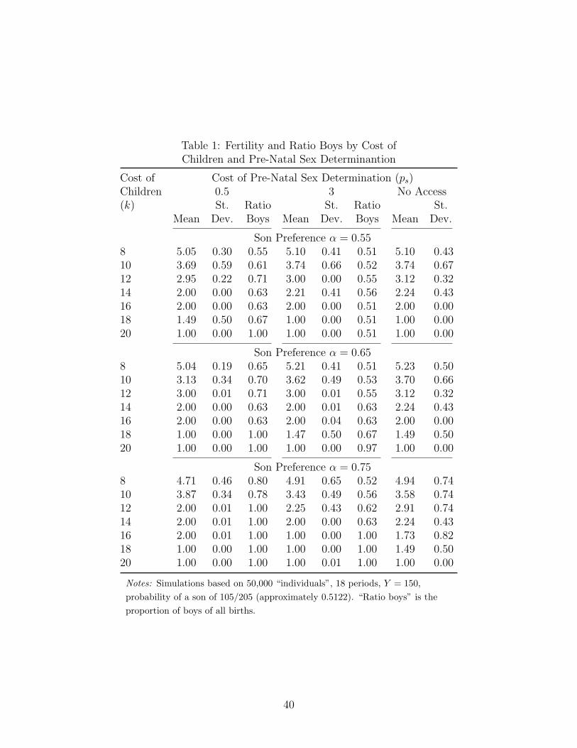
[Table 1 about here.]
16There are three discrete states (boys, girls, scans) and one choice variable with three choices (no preg-nancy, pregancy without pre-natal sex determination, and pregnancy with pre-natal sex determination).Combined with the finite time horizon a problem of this type is especially suited for simulation.
17The last value for the cost of pre-natal sex determination is equivalent to assuming that no pre-natalsex determination is available.
13
[THE FOLLOWING TWO PARAGRAPHS NEEDS A LOT MORE ECONOMIC IN-
TERPRETATION]
Table 1 shows average fertility, the standard deviation of fertility and the ratio of boys to
births for selected values of son preference (α), cost of pre-natal sex determination (ps) and
cost of children (k). While it is often suggested that, in the absense of sex selective abortions,
a stronger preference for sons should lead to higher fertility this is not the case for most of the
specifications used here. Furthermore, even for those cases where there is a positive effect of
stronger son preference on fertility the effect will eventual turn negative once the preference
for son increases beyond a certain point. It is, however, clear that the variance in fertility
increases with stronger son preference, unless children are so expensive that people will
only have one child no matter how strong their son preference is. [IT IS INCONSISTENT
WITH THE ANALYSIS OF THE NON-SSA MODEL ABOVE?] [CHECK ON PREVIOUS
THEORY WORK HERE: STRONGER SON PREFERENCE LEADS TO A DECLINE IN
AVERAGE FERTILITY, BUT ALSO A SUBSTANTIAL INCREASE IN THE VARIANCE
OF FERTILITY. GENERALLY, THEORY SEEMS TO SUGGEST THAT FERTILITY
WILL GO UP.] [fertility for k=4 and a=0.55 is 11.51 fertility for k=4 and a=0.60 is 11.00]
What is especially of interest is what happens when pre-natal sex determination becomes
first available and then cheaper. In general the effect of reducing the cost of pre-natal sex
determination on fertility is negative, although there are situations where fertility goes up,
while the effect on the variance in fertility is uniformly negative. Furthermore, the propor-
tion of boys clearly increases as sex selection becomes less expensive. There is, however, an
interesting twist to the interaction between cost of children and cost of pre-natal sex deter-
mination. While, a priori, one might expect that as children become more expensive there
would be an increase in the proportion of boys Table 1 shows that this is not necessarily
the case. As an example, for moderate son preference (α = 0.55) and relatively expensive
pre-natal sex determination (ps = 3), increasing the cost of children will lead first to a higher
percentage of boys and then to a return to the normal level as fertility falls. [changes in sex
14
ratios for later boys]
[Table 2 about here.]
Table 2 shows the sex ratio, ratio of abortions to births and the average number of
abortions per “individual” for different degrees of son preference and cost of pre-natal sex
determination. All three outcomes increases as the preference for sons becomes stronger
and as the cost of pre-natal sex determination decreases. Furthermore, the lower the cost of
pre-natal sex determination the faster are the increases when son preference strengthens.
[Table 3 about here.]
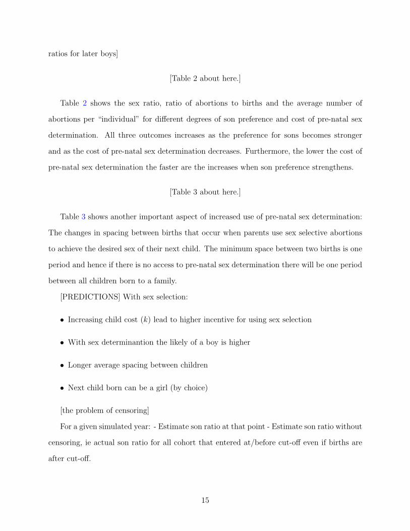
Table 3 shows another important aspect of increased use of pre-natal sex determination:
The changes in spacing between births that occur when parents use sex selective abortions
to achieve the desired sex of their next child. The minimum space between two births is one
period and hence if there is no access to pre-natal sex determination there will be one period
between all children born to a family.
[PREDICTIONS] With sex selection:
• Increasing child cost (k) lead to higher incentive for using sex selection
• With sex determinantion the likely of a boy is higher
• Longer average spacing between children
• Next child born can be a girl (by choice)
[the problem of censoring]
For a given simulated year: - Estimate son ratio at that point - Estimate son ratio without
censoring, ie actual son ratio for all cohort that entered at/before cut-off even if births are
after cut-off.
15
- what happens when son preference is constant, but there is differential access to pre-
natal sex determination? - what are the effects if there is one group with high son preference
and one with low son preference (both have access to sex selection)?
Factors biasing empirical results when sex selection is available: Fewer births in a given
year from people with high son preference; would make the son preference less prominent
(not sure if that works when looking at parities). Of those born to families with high son
preference a higher number are going to be boys; would make the “observed” son preference
higher.
5 Estimation Strategy
[Potential problems] Some contraceptives affects fertility for a long period after. See Dela-
vande, Adeline.
As discussed in Section 4 there are two implications that follows from parents’ decision
to use sex selective abortion. The first is that parents who use ultrasound will have a
higher probability of their next child being a son. The second is that, because there is an
approximately fifty per cent chance of the fetus being female, there should be an additional
waiting time to next birth compared to what is expected when sex selective abortion is not
available. Both of these implications can in principle be tested and used to establish who
uses sex selective abortion. This section discusses the econometric specifications and the
potential problems.
The first method simply consists of estimating the probability of a family having a boy
conditional on a set of explanatory variables. If there is no sex selective abortion this should
be a completely random event and hence there should not be any significant parameters. I
estimate the probability of having a son for parity one through three, both before and after
1985. The choice of 1985 is based on the discussions in Sudha and Rajan (1999). [This
should in principle be done using either logit or probit, but for ease of interpretation I use
16
standard OLS at the moment.]
There are a number of potential estimation issues to consider. First there is the problem
of recall error as discussed above. If a family has a preference for boys and therefore a
higher mortality for girls, then a girl who dies soon after birth is more likely not be reported
and this increases the “probability” of observing a boy instead. Since mortality is likely to
be higher among poorer families this will bias upwards the estimated use of sex selective
abortion among the poor. One way to assess the extent of recall error and for which types of
families it is more likely to be a problem is to use the method described above and estimate
what determines the probability of observing a boy for those births that took place twenty
or more years ago.
Secondly, as discussed above parents may still end up with a girl as their next child even
through they have used sex selective abortion. If this is the case in a substantial number of
households then our estimates may only be a lower bound estimate. This is why the second
method is also of interest since it relies on the duration between births and therefore should
be better at estimating how many abortions there have taken place between two births.
Thirdly, for parity two and above there may be a selection problem. If parents are able
to select the sex of their children or at least abort fetuses of an unwanted sex and the
composition of older siblings are included as an explanatory variables, this may lead to a
bias in the estimates. The same is the case if the samples on which the determinants of the
probability of having a boy are estimated are selected on the basis of the family composition.
For both cases the problem is the difficulty in finding a identifying variables. All variables
that affect the decision on whether to abort a female fetus or not are the same for all parities.
The final problem, and potentially the most serious, the precision and number of data
points needed. In a population with 10,000 births we would expect about 5,122 of them to
be boys in the absence of sex selective abortion. If the use of sex selective abortion drives
the sex ratio up to 110 boys per 100 girls, we would expect 5,238 boys instead. That is only
an increase of 116 boys in a population of 10,000. The implication of this is that the data
17
requirements are relatively intensive and it may be difficult to explain much of the variation
in the sex of the children. It should still, however, be possible to establish which factors have
a significant effect on the probability having a son.
[problems: possibility of genetic differences that affect the likelihood of having a boy;
other methods; unobservable factors that might influence fertility and demand for ultrasound
(such as low fecundity)]
While the first method is in principle easy to implement it may not provide a very precise
estimate of the use of sex selective abortion because it only looks at the birth outcomes. The
second method instead uses the increase in spacing between children that is expected if sex
selective abortion is used. As described above there is at least a three months period between
the beginning of the pregnancy and the time where reliable tests to determine the sex of the
fetus can be carried out. Furthermore, in case a pregnancy is terminated the uterus need at
least two menstural cycles to recover before conception can be attempted again. Finally, the
expected time to conception is about six months. Hence, the use of sex selective abortion is
likely to delay the birth of a child by more than a year.
This “delay” can be used to identify whether sex selection has taken place. Hence, what
is important here is not just the outcome, i.e. whether a girl or a boy is born, but the length
of time until the outcome. The duration between marriage and first birth and between births
partly reflects the strength of demand for a specific outcome.
[CENSORING] [substantial number of observations are censored in that we only ob-
served the time from the last birth but neither the completed length to the next nor the
outcome. This is especially important in this context, where there has been a push towards
lower fertility and where the availability and use of sex selective abortions have increased
duration, hence making censored observations more likely.] [EMPHASISE THE FERTIL-
ITY ASPECT SINCE THIS METHOD CAN TAKE ACCOUNT OF THE FERTILITY
DECISION - CENSORING CAN OCCUR EITHER BECAUSE THEY WANT NO MORE
CHILDREN OR BECAUSE THEY ARE WAITING LONGER/ABORTING MORE]
18
[METHOD] The method used to estimate the duration between births is the discrete
hazard model. A discrete-time approach has two substantial advantages over the standard
continuous time hazard models. First, the duration is measured in months for most of
the sample and while information on the day of birth is sometimes available it is likely to
be measured with more error. Secondly, given that the duration is measured in months a
substantial number of ties (observations with same duration) is likely, which can lead to
serious bias if a Cox proportional hazard model is used. [THIRD ADVANTAGE? Finally, it
is substantially easier to incorporate competing risks and address unobserved heterogeneity.]
[STEPS] Three models are estimated. The first model allows only for the duration from
marriage or previous birth to the next birth or censoring. The second model extends the
first model by explicitly allowing for multiple exit states (boy or girl). The final model
adds unobservable heterogeneity to the second model by looking at repeated spells for each
women. [explain why important - differences in fecundity, demand for boys, etc]
[BASIC MODEL] The basic model examines only the duration between births (or between
marriage and the first birth). For each married woman (i = 1, . . . , n) in the data we observe
at least one spell. All spells are measured in months (t = 1, 2, 3, . . .) and the first spell
begins at the time of marriage and subsequent spells at the birth of a child [OR RISK OF
CONCEPTION?]. The starting point for each spell is t = 1 and it continues until time
ti at which point a birth occurs or the survey takes place (the observation is censored).18
The variable δi is equal to one if i is uncensored (the woman has a child in the given spell);
otherwise it is zero. In addition to information about the spell length there is information
about various individual, household and community characteristics, which included in the
vector of explanatory variable Xit, which may vary with time.
18The time of censoring is assumed independent of the hazard rate as is standard in the literature onhazard models. Furthermore, there is no left censoring in this case since the birth histories are retrospectivefrom the time of marriage.
19
The discrete time hazard rate hit is define as
hit = Pr(Ti = t | Ti ≥ t; Xit), (6)
where T is a discrete random variable that captures the month at which a birth occurs.19 It
is the distribution of T which is of primary interest here. To complete the model specify the
hazard rate as
hit =1
1 + exp (−αt − β′Xit), (7)
or in its logit form
log
[hit
1− hit
]= αt + β′Xit (8)
where αt is the baseline hazard (the hazard when Xit = 0). This is the logistic hazard
model and as shown in Allison (1982) and Jenkins (1995) this specification leads the like-
lihood function to be of the same form as the standard binary logit model, if the data are
transformed so the unit of analysis is spell month rather than the individual woman. In the
reorganised data set the outcome variable is zero if the woman does not have a child in that
month and equal to one if she does have a child in that month. An alternative specification
is the complementary log-log, which is a proportional hazards model. The logistic model
converges to the complementary log-log model if the hazard rate is sufficiently small and
since the logistic model is more easily extendable to more advanced model like multiple exit
states it is preferable here.
To estimate (7) one must also specify the functional form for the baseline hazard function.
The possible forms runs from a simple constant to the completely non-parametric. The non-
parametric consist of as many dummies as there are time periods and is obviously the most
flexible and lead to the best fitting model. The main drawbacks of the non-parametric
version are that it requires events to occcur in each month, that it may fluctuate erratically
across months because of nothing more than sampling variation and that with long spells
19This and the following paragraphs draw on Allison (1982) and Jenkins (1995).
20
it requires inclusion of a large number of unknown parameters. Alternatives to the non-
parametric form is the piece-wise constant baseline hazard rate, which includes dummies
equal to one for months that are expected to have the same hazard, and the polynomial
specifications
αt = α01 +
p∑k=1
αk(t− c)k, (9)
where p decides the order of the polynomial. [THE CHOSEN FORM WILL BE DISCUSSED
IN THE RESULT SECTION BELOW]
[time varying explanatory variables: Changes in sex ratios (probably cannot be identified
because of ten years between censa), changes in legal environment, economic variables)]
[unlikely to be any individual or household specific variables that we can use for time varying
variables]
[MULTIPLE EXIT STATES] While the basic model is a useful starting point and an
improvement on previous studies of what determines sex selective abortions it ignores the
information that comes from the sex of the child when it is born. Loosely speaking if a
son is born after a long spell it provides more evidence of the use of sex selection than if a
girl was born, all else equal. [MODEL PREDICTION OF GIRLS BEING BORN AFTER
LONG SPELLS EVEN WITH PREFECT TECHNOLOGY] [the outcome is an important
aspect, although the model indicates that sex selective abortions can have taken place and
parents can still end up with a girl because the utility of having a girl outweights the cost of
waiting another round - more likely the older the women] Here there are two kinds of events
(j = 1, 2), with one being girl and two boy, and Ji is a random variable indicating which
event took place.20 First, define the discrete time hazard rate for each kind of events
hitj = Pr(Ti = t, Ji = j | Ti ≥ t; Xit). (10)
20In principle a third exit state exists, which is sterilisation [NOT SURE IF ENOUGH INFORMATIONIS AVAILABLE].
21
The logistic model above can be generalised to the following hazard rate
hitj =exp(αjt + β′
jXit)
1 +∑
l exp(αjt + β′lXit)
j = 1, 2. (11)
The advantage of this specification is that it leads the same likelihood function as for a
multinomial logit model in the same way that the basic model lead to the binary logit
model. Hence, it is straigthforward to estimate the case with where the sex of the child born
after a spell is incorporated by multinomial logit procedure. One issue to keep in mind with
this approach is that interpretation of the results is no longer straightforward. First, the
estimated parameters measure the change in probabilities relative to the censored outcome
rather than simply the probability of an event as in the basic model. Secondly, an increase
in a variable with a positive coefficient may not increase the probability that the associated
event occur since the probability of another event(s) may increase even more.21
[problem with IIA assumption (independence of irrelevant alternatives] A more significant
problem with the competing risks model above is that it assumes that alternative exit states
are stochastically independent, also know as the Independence of Irrelevant Alternatives
(IIA) assumption. This rules out any individual-specific unmeasured or unobservable risk
factors that affect both the hazard of having a girl and the hazard of having a boy. In other
words, the assumption requires that the hazard of having a boy relative to not having a
child is uncorrelated with the corresponding relative hazard of having a girl.22 There are
two important factors that are generally unobservable and which may affect both hazards:
Fecundity and the preference for boys. To see how this work, assume that a couple has low
fecundity. This obviously reduces the chance of having a boy, but the assumption requires
that the couple’s chance of having a girl relative to not having a child is the same as for
high fecundity couples which is obviously a very unattractive assumption. In the same
vein, if some couples has very strong preferences for boys the assumption implies that the
21 See Thomas (1996) for an illustration of this problem in a continuous time setting.22See Hill, Axinn, and Thornton (1993) for a more thorough and formal discussion of the issues involved
and a suggested method for estimating a more general model.
22
couples would distribute themselves between having a girl and having no children in the
same proportions as those who had much lower preference for boys. [THIS IS NOT VERY
CLEAR YET]
[ALTERNATIVE TO THE COMPLICATED VERSION BELOW: THE BASIC MODEL
WITH UNOBSERVED HETEROGENEITY]
[REPEATED SPELLS/UNOBSERVABLE HETEROGENEITY] [RANDOM OR FIXED
EFFECTS] [STEELE, DIAMOND AND WANG ’96]
[ISSUES WITH METHOD] [Better health status lead to higher birth hazard, which will
lower the duration between births. Higher demand for sex selective abortion will increase
length. Over the time period covered by the data there has been both increased health of
women and higher demand for sex selective abortion. The better health will, all else equal,
bias downward the estimates and make it more difficult to find evidence of sex selective
abortion. A related issue is increased labour force participation which may also affect the
spacing between children, independently of the demand for sex selective abortions]
6 Data
The data come from the three rounds of the National Family Health Survey (NFHS-1, NFHS-
2 and NFHS-3), collected in 1992-93, 1998-99 and 2005-2006, respectively.23 All are based on
the Demographic and Health Survey Model B, with NFHS-1 using the DHS II questionnaire
while NFHS-2 and NFHS-3 using, respectively, the DHSIII questionnaire and the Measure
DHS questionnaire. All three surveys are large: NFHS-1 covered 89,777 ever-married women
aged 13-49 from 88,562 households, NFHS-2 covered 90,303 ever-married women aged 15-49
from 92,486 households and NFHS-3 covered 124,385 never-married and ever-married women
aged 15-49 from 109,041 households. They were collected by the International Institute for
Population Sciences in Mumbai and have nationwide coverage.
23 NFHS-2 also has a small number of observation collected in 2000, due to a delay in the survey forTripura.
23
[VARIABLES - DEPENDENT]
[ISSUES] NFHS-1 is missing detailed information on the timing of marriage (gauna issue)
and spacing since partners began living together to first birth [NEED TO EXPAND ON
THIS]
[VARIABLES - INDEPENDENT]
In 2000 three new states were created in India: Uttaranchal, Jharkhand and Chhattis-
garh. To ensure consistency across the three surveys each are included in the state these
areas used to belong to.24
While the first round of the NFHS asked only about membership of either a scheduled
caste or tribe the later rounds were expanded to also ask about membership of other backward
castes. To ensure consistency the only two variables used are dummies for whether a woman
belongs to a scheduled caste or a scheduled tribe, respectively. Another question that has
been changed from the first round is on religion. The NFHS-1 only gave five options (Hindu,
Muslim, Christian, Sikh and Other), while NFHS-2 and NFHS-3 had twelve and elleven
options, respectively. I use seven dummies for religious affiliation (Hindu, Muslim, Christian,
Sikh, Buddhist, Jain and Other25) with “Other” being the excluded category. While this
means that some of the women from NFHS-1 that are either Buddhist or Jain will be
included in the category “Other” because those categories were not available these groups
are important enough in terms of size and/or expected effect that they are still included.
[DATA REDUCTION - FINAL SAMPLE] In NFHS-1 a total of 89,777 women were
interview. Out of those 6424 were visitors to the household in which they were interviewed
and therefore dropped. Furthermore, 1538 women who has been married more than once
were dropped and 42 were dropped because they had inconsistent information on their age
of marriage.26
24Uttaranchal was formerly part of Uttar Pradesh, Jharkhan was part of Bihar and Chhattisgarh was partof Madhya Pradesh.
25Included in “Other” are Jewish, Parsi/Zoroastrian, Doni-Polo, Sanamahi and no religion.26Dropping the latter is necessary in NFHS-1 because it, contrary to NFHS-2 and NFHS-3 do not calculate
month of marriage and it therefore had to be imputed from age at first marriage.
24
In NFHS-2 a total of 90,303 were interviewed, with 5955 dropped since they were visitors
and 1569 because they were married more than once.
Finally, 124,385 women were originally interviewed in NFHS-3. Of those, 5528 are deleted
here since they were visitors and 29,668 because they were never married.27 Furthermore,
1994 were excluded since they had been married more than once.
Both the mother’s and the father’s education is measured in years. All observations
where the education of the mother is missing are dropped.28
3147 women were dropped since they had at least one set of multiple births leaving a
total sample of 191,883 women.
[DROPPED BECAUSE TOO SHORT SPACING]
6.1 Recall Error and the Sex Ratio
Among the preliminary work done is an analysis of the extent to which the birth histories
collected are reliable. This is an important first step since the estimation methods proposed
in “Research Design and Methods” rely on good quality data on both the sex of children
born and the spacing between these children.29 What is especially of concern is the potential
for recall error, i.e. children who are missed during the collection of a woman’s birth history,
for example, because of those children’s early death. In recognition of this problem, the
DHS III schedule, which is used for NFHS-2 and NFHS-3, has the interviewer probe about
any missed births if there is four or more years between two births reported as consecutive.
While probing helps catch many originally missed births, recall error is still likely to be a
substantial problem in India. First, there is a significantly higher mortality risk for girls
than for boys. Secondly, the preference for boys may also lead to more boys than girls
27The latter category also include married women if gauna had not been performed at the time of thesurvey.
28In NFHS-1 253 observations are dropped, while 36 and 6 are dropped from NFHS-2 and NFHS-3,respectively.
29The same is the case for analyses of the determinants of child mortality but relatively little attentionhas been paid to this problem despite the potential for substantially underestimating mortality, especiallyfor girls.
25
being remembered among those children who died early. Finally, the probing works of long
intervals between observed births, but given short durations between births, especially after
the birth of a girl, it is unlikely to pick up all children.
[Figure 2 about here.]
That differential recall of boys and girls is, indeed, a problem can be seen from Figure
3. The solid line shows the ratio of boys to children reported as first born by the number
of years between the survey and the year of marriage of the parents, while the dashed lines
indicate the 95% confidence interval. For comparison the figure also include the natural ratio
of boys (approximately 0.512 or 105 boys per 100 girls). Clearly the observed ratio of boys is
increasing likely to be above the expected value the further the parents’ marriage was from
the survey. For comparison consider that a ratio of 0.55 is equivalent to a sex ratio of about
120 boys to 100 girls. Since pre-natal sex determination techniques did not become widely
available until mid-eighties this cannot explain the higher sex ratio. Recall error makes an
analysis of the spread of sex determinations techniques less precise, since there may appear
to be little change in the sex ratio over time even though the actual sex ratio at birth has
increased. It also makes it more difficult to identify which families are using sex selective
abortions. One solution is to drop observations which are too far away from the survey year.
For the preliminary results presented in the following section all women who were married
22 years or more at the time of the survey were excluded.
7 Results
For the moment I have chosen the following explanatory variables. For both the mother and
the father I have divided their education into five group: No education, which is the excluded
variable, 1 to 5 years of education, 6 to 9 years of education, 10 to 14 years of education
and finally 15 or more years of education. There are three land variables used. A dummy
for whether the household own any agricultural land, which is used for urban households
26
and the number of acres of irrigated and non-irrigated land the household own. The latter
two are used for rural households. The predominate religion in India is Hindi, which is the
excluded religion variable. There are also dummies for being Muslim, Christian, Sikh and
others.
For urban household the place of residence can be located in either a large or capital city,
the excluded variable, or in a small city or a town. The geographical dummies follow those
used above. The ratio of the mean of women’s education over men’s education is supposed
to measure equality of the sexes until a better variable can be found (see below).
There is three dummies for year of birth: 1985-1989, which is the excluded variable,
1990-1994 and 1995-1999. Furthermore, the variable “No Boys” takes the value one if there
are no surviving boys at the time of birth of the child in question. Likewise, “One Boy” take
the value one if there is exactly one boy alive at the time of birth of the child. Both of these
refer only to older siblings; multiple births have been dropped from the sample.
There are a number of variables that it would be of great interest to include. One is
some measure of the relative return to investing in boys versus girls. An example could be
the relative wage rate between women and men as used in Rosenzweig and Schultz (1982),
although this may actually measure the relative bargaining power of women and not the
return to investment.
Another variable is one that can capture the ”feedback mechanism” from a changing sex
ratio on the use of sex selective abortions. At one point parents must realise that the current
dowry system will not continue, which must affect the demand. A possible measure of this
could be the ratio of marriage-aged girls to marriage-aged boys [census?]. Furthermore, it
may be possible to trace the effect of making the use of ultrasound for sex determination
illegal
There are variables which have been excluded even through they seem appropriate at
first glance. Chief among these is measures of son preference. I tried two measure: Whether
the family wants more boys than girls and whether it wants more than half their children
27
to be boys. The reason for excluding these measures is evidence of a very strong effect from
actual sex composition of children to these measures.
Related to this is the exclusion of a number of wealth variables that turned out to be
endogenous. An example is livestock, which, if included, is very significant in the 1970-1984
sample of rural households when looking at first borns, while nothing else is. That must
be because those household that were “lucky” enough to have a son (as first born) in the
period 1970-84 can now cash in on their dowry (which may be in the form of livestock or
be converted to livestock). It is an open question whether the land variable suffer from the
same problem, but it appears to be of a lesser degree if it does.
7.1 Spacing between Births
The proposed method take as its starting point the predicted increase in spacing between
births from increased access to sex selective abortion. There is at least a three months period
between conception and when reliable tests to determine the sex of the foetus can be carried
out. Furthermore, in case a pregnancy is terminated the uterus need at least two menstrual
cycles to recover before conception can be attempted again. Finally, the expected time to
conception is about six months. Hence, one sex selective abortion is likely to delay the birth
of the next child by a year. This “delay” can be used as part of the identification of whether
sex selection has taken place. What is important is not just the outcome, i.e. whether a girl
or a boy is born, but also the duration.
The econometric model suggested for analysing spacing is the discrete hazard model,
which has a number of advantages. First, compared to non-hazard models, hazard models
automatically accounts for censoring. Secondly, while the underlying process is in continuous
time the observed interval is only reliably measured in months. This makes a discrete hazard
model more attractive since a substantial number of ties (observations with same duration) is
likely, which lead to bias in continuous time models like the Cox proportional hazard model.
Finally, it is relatively easy to estimate and to incorporate unobserved heterogeneity. Three
28
models are proposed. The first model looks only at the duration of the spells. The second
model extends the first by explicitly allowing for multiple exit states (boy or girl). The final
model adds unobservable heterogeneity by looking at repeated spells, which can be done for
all women who had at least one birth.
The basic model examines only the duration between births (or between marriage and
the first birth), which allows us to understand how the spacing between births has changed
with the introduction of sex selective abortions. For each married woman (i = 1, . . . , n) in
the data we observe at least one spell. All spells are measured in months (t = 1, 2, 3, . . .)
and the first spell begins at the time of marriage and subsequent spells at the birth of a
child plus eight months. The starting point for each spell is t = 1 and it continues until time
ti at which point a birth occurs or the survey takes place (the observation is censored).30
In addition to information about the spell length and censoring status there is information
about various individual, household and community characteristics, which are included in
the vector of explanatory variable Xit. These will be discussed below.
The discrete time hazard rate is define as hit = Pr(Ti = t | Ti ≥ t; Xit), where T is a
discrete random variable that captures the month at which a birth occurs. To complete the
model specify the hazard rate as
hit =1
1 + exp (−αt − β′Xit), (12)
where αt is the baseline hazard (the hazard when Xit = 0). This is the logistic hazard model
and as shown in Allison (1982) and Jenkins (1995) this specification has the same likelihood
function as the standard binary logit model. Hence, if the data are transformed so the unit
of analysis is spell month rather than the individual woman the model can be estimated
using a standard logit model. In the reorganised data set the outcome variable is zero if
the woman does not have a child in that month and one if she does have a child in that
30The time of censoring is assumed independent of the hazard rate as is standard in the literature onhazard models. Furthermore, there is no left censoring in this case since the birth histories are retrospectivefrom the time of marriage.
29
month. The logistic model converges to the complementary log-log model if the hazard rate
is sufficiently small and since the logistic model is more easily extendible to advanced model
like multiple exit states it is preferable here.
While the basic model is a useful starting point, it ignores the information from the sex of
the child who is born at the end of a completed spell. This information can be incorporated
by using a competing risk model. Here there are two exits (j = 1, 2), with one being girl
and two boy, and Ji is a random variable indicating which event took place.31 Define the
discrete time hazard rate for each kind of events: hitj = Pr(Ti = t, Ji = j | Ti ≥ t; Xit). The
logistic model above can then be generalised to the following hazard rate
hitj =exp(αjt + β′
jXit)
1 +∑
l exp(αjt + β′lXit)
j = 1, 2. (13)
The advantage of this specification is that it leads to the same likelihood function as for a
multinomial logit model. Hence, it is straightforward to estimate using multinomial logit
on the individual months. One drawback is that interpretation of the results is no longer
straightforward. First, the estimated parameters measure the change in probabilities relative
to the base outcome (here no birth) rather than simply the probability of an event as in the
basic model. Secondly, an increase in a variable with a positive coefficient may not increase
the probability that the associated event occur since the probability of the other event may
increase even more.32
A more significant problem is that it assumes that alternative exit states are stochastically
independent, also know as the Independence of Irrelevant Alternatives (IIA) assumption.
Even though boys and girls are clearly not perfect substitutes they are very similar and
this presents a problem for the IIA assumption. Furthermore, the assumption also rules out
any individual-specific unmeasured or unobservable risk factors that affect both the hazard
of having a girl and the hazard of having a boy. In other words, the assumption requires
31A third exit state, sterilisation, exists and will be incorporated if sufficient data is available.32See Thomas (1996) for an illustration of this problem in a continuous time setting.
30
that the hazard of having a boy relative to not having a child is uncorrelated with the
corresponding relative hazard of having a girl.33 There are two important factors that are
generally unobservable and which may affect both hazards: Fecundity and the preference for
boys. As an example, assume that a couple has low fecundity. This reduces the chance of
having a boy, but the assumption requires that the couple’s chance of having a girl relative
to not having a child is the same as for high fecundity couples which is obviously a very
unattractive assumption. In the same vein, if some couples has strong preferences for boys,
the assumption implies that these couples would distribute themselves between having a girl
and having no children in the same proportions as those who had much lower preference for
boys if access to sex selective abortion disappeared.
The final model therefore expands the competing risk model to include unobserved het-
erogeneity. This is possible since we observe more than one spell for most women. Steele,
Diamond, and Wang (1996) suggest a random-effect discrete-time competing-risk hazard
model that will be the basis for this effort. Including a random effect can control both for
unobserved heterogeneity and for possible correlation between durations between births for
women who contribute multiple spells. This is important since this would be one way of not
confusing families who have stopped child bearing with those currently using sex selective
abortions.
The same set of explanatory variables will be used for all three models and the models
will be estimated for all spells. The explanatory variables can be divided into household
variables and area characteristics. The explanatory variables at the household level are the
education and age of the mother and father, land ownership, religion, whether the household
belongs to a scheduled tribe or caste and the sex composition of previous children.
The mother’s education is one of the main determinants of the opportunity cost of fertility
and hence higher education is expected to lead to lower fertility. This in turn should increase
the use of sex selective abortions for a given level of son preference. The father’s education
33See Hill, Axinn, and Thornton (1993) for a more thorough and formal discussion of the issues involvedand a suggested method for estimating a more general model.
31
is mainly associated with higher income which should lead to higher fertility, but the effect
on the use of sex selective abortions is ambiguous. On one hand, the higher fertility might
lead to lower use of sex selective abortions. On the other hand, the higher income also makes
using sex selective abortion more affordable. In previous research, the sex composition of
previous children is the one set of variables that have shown a significant effect on sex
selective abortion. The expected effect of having more girls for a given number of children
is increased use of sex selective abortions. The sex composition variables will be interacted
with parental characteristics and other explanatory variables to examine how the effect of
composition vary with household characteristics.34
The area characteristics include area of residence, sex ratio, relative education levels
between men and women and region. The area of residence (city, large town, small town,
rural) captures both access to pre-natal sex determination techniques and the cost of children.
Moving from rural to more urban area should increase both the cost of children and access
to pre-natal sex determination. Both are expected to lead to greater use of sex selective
abortions. The ratio of marriage-aged girls to marriage-aged boys is included to capture
the potential “feedback mechanism” from a changing sex ratio on the use of sex selective
abortions. Although the lack of girls might in principle decrease the use of sex selective
abortions, the availability of brides from outside the area is likely to dampen this effect.
Finally, the relative education levels of men and women can serve as a proxy for women’s
opportunities and/or return to investment in human capital. The expected effect of an
increase in women’s education relative to men’s is to lower the use of sex selective abortion.
For all three models one must also specify the functional form for the baseline hazard
function. The possible forms range from a simple constant to the completely non-parametric.
The non-parametric consist of as many dummies as there are time periods and is obviously
34Note that in principle there may be an endogeneity problem for the sex composition variable since withaccess to sex selective abortion the composition is a choice variable. Hence, including composition as anexplanatory variable may lead to biased estimates. The problem is finding identifying variables since all othervariables that affect the decision on whether to abort a female foetus or not are the same for all parities.This problem will be addressed in future research.
32
the most flexible and lead to the best fitting model. The main drawbacks of the non-
parametric version are that it requires events to occur in each month, that it may fluctuate
erratically across months because of nothing more than sampling variation and that with
long spells it requires inclusion of a large number of parameters. Alternatives to the non-
parametric form is the piece-wise constant baseline hazard rate, which includes dummies
equal to one for months that are expected to have the same hazard, and various polynomial
specifications. Royston and Sauerbrei (2008) propose a method that can help specify the
baseline hazard function using fractional polynomials. The fractional polynomials method
has the advantages of flexibility and that it can be used to extend the hazard models to
be non-proportional by interacting the baseline hazard with explanatory variables such as
the sex composition of previous children.35 This allows the functional form of the hazard in
question to depend directly on the sex of previous children.
[Figure 3 about here.]
To illustrate the method, preliminary results are presented using multinomial logit to
incorporate competing risks. Time is measured in quarters and the baseline proportional
hazard function is estimated using fractional polynomials. The estimations are done for
the second spell, which is the spell after the first birth, for the time periods: 1972-1984,
1990-1994 and 1995-2006.36 Using the multinomial estimation results, one can predict the
probability of having a child of a specific sex in a given quarter (conditional on not having
had a child already). The advantage of this is that the relative probability of having a boy vs
a girl is the predicted sex ratio while taking account of censoring. Furthermore, confidence
intervals can be calculated using the delta method. Figure 4 shows the sex ratio (divided
by 100) with 90% confidence intervals for three levels of education (assumed the same for
wife and husband) for a Hindu family, who had a girl as their first child, lives in a large city,
35The downside is that with a large number of observations and long spells the computing requirementsbecome substantial. Finding the baseline hazard for the preliminary results took up to 8 hours on a fastserver.
36The number of observed quarters are 410,878, 297,590 and 321,287, respectively.
33
have no land and are not part of a scheduled tribe or caste. Each column represents a time
period. Furthermore, the sex ratio of 105 is shown as the horizontal solid line.
The left column shows that, as expected, there is no evidence of the use of sex selective
abortion in the period before 1985. The predicted sex ratios are not statistically significantly
different from 105 at any point and for 6 and 12 years of education they are essentially
identical to the expected value. The picture is very different for the middle column, which
shows spells that begun in 1990-1994 period. Those with high education now have a predicted
sex ratio which is statistically significantly higher than the natural until about 20 quarters
from the first birth. Furthermore, the ratio is large at around 130, which is especially
noteworthy since these estimations use data from all of India, not just the northern states.
There is little evidence of the use of sex selective abortion among those with lower education
for this period. Finally, in the last column, which covers spells begun in the period 1995-
2006, even the sex ratio among those with no education is statistically significant for at least
part of spell and it very statistically significant for the 6 and 12 years groups. The predicted
sex ratio for those with 12 years of education is now up to around 140 boys per 100 girls.
As predicted the likelihood of using sex selective abortions becomes smaller the longer the
duration from the first child. Other preliminary results show that the sex composition of
children is a strong driver of the use of pre-natal sex selection, but more importantly this
effect increases with level of education. As an example, the predicted sex ratios, equivalent
to those in Figure 4, with the first child a boy instead of a girl show little evidence of the
use of sex selective abortion, even for those with 12 years of education in the 1995-2006
time period. This is consistent with strong son preference combined with a lower desired
fertility for higher levels of education. Finally, it is worth noting that that spacing after
a girl becomes significantly longer with access to sex selective abortion, which may have
important effects on the girls survival chances since she is now less likely to have to compete
for resources.
Finally, factors other than sex selective abortions clearly affect the hazard of having a
34
birth. Two examples are the health status of the mother and the use of contraceptives.
Better health status lead to a higher chance of conception and of carrying the pregnancy to
term, which will lower the duration between births, while the use of contraceptive has the
opposite impact since it reduces the hazard of a birth. If one used only the first model, these
factors could influence the results by making it appear less or more likely that sex selection
has taken place. This is why the proposed second and third models are important. They
utilise the differences in the hazards of having a boy vs a girl while still taking account of
censoring. As illustrated by Figure 4 these models provide direct evidence on the use of sex
selective abortions. The combination of outcome and duration is what makes the proposed
methods especially appealing.
8 Conclusion
[to be added] In summary, the purpose of this project is to develop an empirical method that
can contribute to an understanding of the changing sex ratio at birth in India. Beside being
of intrinsic interest, this first step is likely to have a significant impact on future analyses
in areas such as child health and mortality, maternal mortality, female abandonment and
changes in the marriage markets. These are important areas for future research.
35
References
Ahn, N. (1995): “Measuring the Value of Children by Sex and Age Using a Dynamic
Programming,” Review of Economic Studies, 62(3), 361–79.
Allison, P. D. (1982): “Discrete-Time Methods for the Analysis of Event Histories,”
Sociological Methodology, 13, 61–98.
Arnold, F., M. K. Choe, and T. K. Roy (1998): “Son Preference, the Family-Building
Process and Child Mortality in India,” Population Studies, 52(3), 301–15.
Bloch, F., and V. Rao (2000): “Terror as a Bargaining Instrument: A Case Study of
Dowry Violence in Rural India,” Policy Research Working Paper 2347, World Bank.
Cain, M. (1981): “Risk and Insurance: Perspectives on Fertility and Agrarian Change in
India and Bangladesh,” Population and Development Review, 7(3), 435–474.
(1983): “Fertility as an Adjustment to Risk,” Population and Development Review,
9(4), 688–702.
(1990): “Risk and Fertility in a Semi-Feudal Context: The Case of Rural Madhya
Pradesh,” Research Division Working Paper 19, The Population Council.
Chu, J. (2001): “Prenatal Sex Determination and Sex-Selective Abortion in Rural Central
China,” Population and Development Review, 27(2), 259–81.
Das Gupta, M., and P. N. M. Bhat (1997): “Fertility Decline and Increased Manifes-
tation of Sex Bias in India,” Population Studies, 51(3), 307–15.
Davies, J. B., and J. Zhang (1997): “The Effects of Gender Control on Fertility and
Children’s Consumption,” Journal of Population Economics, 10(1), 67–85.
Deolalikar, A. B., and V. Rao (1998): “The Demand for Dowries and Bride Char-
acteristics in Marriage: Empirical Estimates for Rural South-Central India,” in Gender,
36
Population and Development, ed. by M. Krishnaraj, R. M. Sudarshan, and A. Shariff, pp.
122–140. Oxford University Press, Delhi; Oxford and New York.
Dyson, T. (2001): “The Preliminary Demography of the 2001 Census of India,” Population
and Development Review, 27(2), 341–56.
Edlund, L. (1999): “Son Preference, Sex Ratios, and Marriage Patterns,” Journal of Po-
litical Economy, 107(6), 1275–1304.
Foster, A. D., and M. R. Rosenzweig (1999): “Missing Women, the Marriage Market
and Economic Growth,” Manuscript, Brown University.
Goodkind, D. (1996): “On Substituting Sex Preference Strategies in East Asia: Does
Prenatal Sex Selection Reduce Postnatal Discrimination,” Population and Development
Review, 22(1), 111–25.
Haughton, J., and D. Haughton (1998): “Are Simple Tests of Son Preference Useful?
An Evaluation Using Data from Vietnam,” Journal of Population Economics, 11(4), 495–
516.
Hill, D. H., W. G. Axinn, and A. Thornton (1993): “Competing Hazards with Shared
Notes: Simulations based on 50,000 “individuals”, 18 periods, Y = 150,probability of a son of 105/205 (approximately 0.5122). “Ratio boys” is theproportion of boys of all births.
40
Table 2: Sex Ratios and Abortions by Cost ofPre-Natal Sex Determination and Son Preference
Son Cost of Pre-Natal Sex Determination (ps)Preference No(α) 0.5 1 2 3 Access
Notes: Simulations based on 50,000 “individuals”,18 periods, Y = 150, k = 8, probability of a sonof 105/205. Minimum space is 1 period.
42
n=0bbbbbbbbbbbbbbbbbbbbbbbbb
\\\\\\\\\\\\\\\\\\\\\\\\\
t=1 -Seeeeeeeeeeeee
YYYYYYYYYYYYY Seeeeeeeeeeeee
YYYYYYYYYYYYY
bjjjjjjj
TTTTTTT gjjjjjjj
TTTTTTT 0 0jjjjjjj
TTTTTTT bjjjjjjj
TTTTTTT
t=2 -Svvv
v IIII S
vvvv IIII -S
vvvv IIII S
vvvv IIII -S
vvvv IIII S
vvvv IIII -S
vvvv IIII S
vvvv IIII
bb bg b b bb gb gg g g gb g b 0 0 b bb bg b b bb
Figure 1: Decision Tree for a Two Period Model with Pre-natal Sex Screening
43
33.
54
4.5
55.
5
1950 1960 1970Respondent’s year of birth
Figure 2: Children Ever Born atAge 35
.48
.5.5
2.5
4.5
6.5
8.6
0 10 20 30Years between marriage and interview
Figure 3: Ratio of Boys for “First”Births
44
.81
1.2
1.4
1.6
0 5 10 15 20Quarter
(a) No education
.81
1.2
1.4
1.6
0 5 10 15 20Quarter
(b) No education
.81
1.2
1.4
1.6
0 5 10 15 20Quarter
(c) No education
.81
1.2
1.4
1.6
0 5 10 15 20Quarter
(d) 6 years
.81
1.2
1.4
1.6
0 5 10 15 20Quarter
(e) 6 years
.81
1.2
1.4
1.6
0 5 10 15 20Quarter
(f) 6 years
.81
1.2
1.4
1.6
0 5 10 15 20Quarter
(g) 12 year
.81
1.2
1.4
1.6
0 5 10 15 20Quarter
(h) 12 year
.81
1.2
1.4
1.6
0 5 10 15 20Quarter
(i) 12 year
Figure 4: Predicted Sex Ratios by Spacing after First Birth for a Family with 1 Girl.Time Periods in Columns: Left, before 1985; Middle, 1990-94; Right, 1995-2006.Education Levels in Rows: Top, No Education; 2nd, 6 Years; Bottom, 12 Years.