The Discontinuous Galerkin Method for Conservation Laws Michael, Crabb 2010 MIMS EPrint: 2015.63 Manchester Institute for Mathematical Sciences School of Mathematics The University of Manchester Reports available from: http://eprints.maths.manchester.ac.uk/ And by contacting: The MIMS Secretary School of Mathematics The University of Manchester Manchester, M13 9PL, UK ISSN 1749-9097
Transcript
The Discontinuous Galerkin Method forConservation Laws
Michael, Crabb
2010
MIMS EPrint: 2015.63
Manchester Institute for Mathematical SciencesSchool of Mathematics
The University of Manchester
Reports available from: http://eprints.maths.manchester.ac.uk/And by contacting: The MIMS Secretary
5.8 2D dam-break - Comparison of average height solutions using the FVM
and DGFEM for elements lying on the x-axis . . . . . . . . . . . . . 75
5.9 2D dam-break - Comparison of average height solutions using the FVM
and DGFEM for elements lying on the y-axis . . . . . . . . . . . . . . 75
5.10 2D dam-break - Comparison of average height solutions using the FVM
and DGFEM for elements lying on the line y = x . . . . . . . . . . . 75
5.11 2D dam-break - Comparison of the average DGFEM height solution,
near the shock, along the x-axis, y-axis and line y = x . . . . . . . . . 76
7
The University of Manchester
Michael CrabbMaster of ScienceThe Discontinuous Galerkin Method For Conservation LawsOctober 14, 2010
The aim of this project is to study discontinuous Galerkin methods applied to coupledsystems of partial differential equations in conservative form in 1D and 2D.
In 1D, a formulation was successfully implemented to solve continuous problemsfor the advection and shallow water equations. Discontinuous problems for the in-viscid Burgers’ equation and a breaking dam problem were also investigated and theeffectiveness of h- and p-refinement discussed. An alternate set of shallow water equa-tions were derived yielding equivalent results for a continuous problem but differentnumerical solutions for the breaking dam problem. These anomalous results highlightthe importance of enforcing conservation of the correct conserved physical variablesin cases when solutions exhibit shocks.
A 2D slope limiter, applicable to quadrilateral elements, is implemented and nu-merical results obtained for a smoothed breaking dam problem in 2D. A comparisonis made between these results and those from a finite volume method (results byChris Johnson) and indicate that, for this particular problem, both methods resolvethe shock over the same length scale.
8
Declaration
No portion of the work referred to in this dissertation has
been submitted in support of an application for another
degree or qualification of this or any other university or
other institute of learning.
9
Copyright Statement
i. Copyright in text of this dissertation rests with the author. Copies (by any
process) either in full, or of extracts, may be made only in accordance with
instructions given by the author. Details may be obtained from the appropriate
Graduate Office. This page must form part of any such copies made. Further
copies (by any process) of copies made in accordance with such instructions
may not be made without the permission (in writing) of the author.
ii. The ownership of any intellectual property rights which may be described in
this dissertation is vested in the University of Manchester, subject to any prior
agreement to the contrary, and may not be made available for use by third
parties without the written permission of the University, which will prescribe
the terms and conditions of any such agreement.
iii. Further information on the conditions under which disclosures and exploitation
may take place is available from the Head of the School of Mathematics.
10
Acknowledgements
A special thank you to my supervisor, Dr. Andrew Hazel, for developing my under-
standing of the oomph-lib and for his useful discussions and comments during the
past five months. I would also like to thank Prof. Matthias Heil for his help during
the project and Chris Johnson for his two dimensional dam-break results, which were
essential for validation of my computational results.
11
Abbreviations
The following abbreviations are commonly used in this report:
• DG - Discontinuous Galerkin.
• FEM - Finite element method.
• FVM - Finite volume method.
• PDE - Partial differential equation.
• ODE - Ordinary differential equation.
• GLL - Gauss-Lobatto-Legendre.
• RK - Runge-Kutta.
• CFL - Courant-Friedrichs-Levy.
• TVDM - Total variation diminishing in the means.
• TVBM - Total variation bounded in the means.
12
Chapter 1
Introduction
1.1 Conservative PDEs in one dimension
In this report, coupled systems of partial differential equations (PDEs) in conservative
form will be studied. First, consider a system of one conserved field, w, in one spatial
dimension, x. A simple conservation law for this single field states that “the rate
of change of the total amount of w inside a region [L,R] equals the amount of w
that flows into [L,R] minus the amount that flows out of [L,R]”. This statement is
expressed mathematically below, where f represents the flux, or flow, and t is the
time:
d
dt
∫ R
L
w(x, t) dx = f(L, t)− f(R, t). (1.1)
If f is continuously differentiable, then the integral form (1.1) can be written
d
dt
∫ R
L
wdx = −∫ R
L
∂f
∂xdx,
and if the field, w, is continuously differentiable we can write∫ R
L
(∂w∂t
+∂f
∂x
)dx = 0.
The integral above is true for any control region [L,R] and this is only possible if the
integrand equals 0. We recover the PDE form of the conservation law,
∂w
∂t+∂f
∂x= 0. (1.2)
13
CHAPTER 1. INTRODUCTION 14
1.2 Abstract system of conservative PDEs
Systems of PDEs relating m conserved fields in n spatial dimensions will be consid-
ered. In the spirit of the 1D conservation law (1.2), a general system of conserved
PDEs can be written in the form,
∂w(x, t)
∂t+∇.F (w(x, t),x, t) = 0 x ∈ Ω, (1.3)
where Ω ⊂ Rn is the problem domain, x ∈ Ω is a spatial location, t is the time,
w ∈ Rm is a vector of the unknown fields and F ∈ Rm×n is the flux matrix. The
Roe [9] solved a linearised version of the Riemann problem, at each element edge,
to find a field that approximately solves the Riemann problem and hence determine
a numerical flux. He introduced so called Roe average states, and used the jump
conditions at the discontinuity (see equation (4.17)), to find approximate solutions
to the Riemann problem. Specifically, for the shallow water equations in 1D (3.9),
this flux can be written in the form,
f∗RA(w−h (x),w+h (x)) = f∗CEN(w−h (x),w+
h (x))− CRA2
(w+h (x)−w−h (x)), (2.11)
where CRA is the Roe average constant. For the shallow water equations, the con-
served field is w = (h, hu)T , and by introducing the Roe average states at each edge,
h =h− + h+
2, u =
√h−u− +
√h+u+√
h− +√h+
, (2.12)
CHAPTER 2. PRELIMINARIES 22
the constant is calculated as
CRA = maxh,u|u±√gh|, (2.13)
which is a simple optimization problem over two different values. For further details
of the theoretical justification of this numerical flux see [4, 9, 10].
A general implementation of the numerical flux into the oomph-lib is described in
more detail in Appendix B.
2.3 Elemental linear system
Returning to the weak form (2.4) and substituting the local solution approximation
in element e (2.2), there are Np equations to be solved for each component of the
field corresponding to the values at the Np grid points,∫De
∂wj
∂tlj(x)li(x)dx =
∫De
F.∇li(x)dx−∫∂De
f∗li(x)dx i = 1 : Np, (2.14)
where wj is a vector of the unknown fields at the nodal position xj. Using the Einstein
summation convention, it is useful to define an element mass matrix, M , flux matrix,
F , and numerical flux matrix, F ∗:
Mki =
∫De
lk(x)li(x)dx k, i = 1 : Np (2.15)
Fki =
∫De
Fkj∂li(x)
∂xjdx i, j = 1 : Np k = 1 : m (2.16)
F ∗ki =
∫∂De
f ∗k li(x)dx i = 1 : Np k = 1 : m (2.17)
Equation (2.14) is equivalent to a system of m × Np ordinary differential equations
(ODEs), that must be solved in every element. These ODEs can be written in the
form, M 0 0
0. . . 0
0 0 M
w1
...
wm
=
f1
...
fm
+
g∗1...
g∗m
, (2.18)
where M is the element mass matrix defined in (2.15) and the vectors fi and g∗i are
the ith column of the flux and numerical flux matrices defined in (2.16) and (2.17)
CHAPTER 2. PRELIMINARIES 23
respectively. wi is a vector of the nodal values across the element corresponding to
the ith field1.
2.3.1 Element coupling and boundary conditions
In the elemental linear system (2.18) the only communication between elements is
through the evaluation of the numerical flux matrix (2.17). The entries of this matrix
are line integrals of the numerical flux along the element boundary and so coupling
is required between adjacent faces in the mesh.
In the implementation, for 2D rectangular elements, every element in the mesh,
named a bulk element, is assigned an index e. Every bulk element is assigned a
pointer to each of the four faces, named face elements, and on each of these faces, a
pointer is assigned to the neighbouring face. In every bulk element the entries of the
numerical flux matrix are computed by moving to one of the faces, finding this face’s
neighbour, and then evaluating the numerical flux at every integration knot point
along the face as illustrated in figure 2.2. See section 2.4 for integration scheme.
Figure 2.2: The figure illustrates a rectangular (bulk) element in the mesh, O, and it’sneighbours N , E, S and W . One of the faces F (OS) and its neighbouring face F (SO) areillustrated along with the numerical flux integration knot points (squares) along the edge fora Q4 finite element (bi-cubic approximation).
1The superscript notation for the unknowns, wi i = 1 : m, corresponds to a vector of unknownsacross the nodal positions of the element for a given field component i, whereas the subscriptnotation, wj j = 1 : Np, corresponds to a vector of the unknown fields at a given nodal point xj
CHAPTER 2. PRELIMINARIES 24
Boundary Conditions
For an element lying on the domain boundary, one or more of the faces also lies on the
domain boundary and so there is no neighbouring face to assign a pointer to. This
is not a problem for periodic boundary conditions because the neighbouring face is
simply set as the face on the opposite side of the mesh.
For Dirichlet boundary conditions the field at the boundary is known. The pointer
to the neighbouring face is set to point to the face element itself. This ensures the
numerical flux function will return the physical normal flux, f∗(w,w) = F (w).n,
because of the second property of a numerical flux in section 2.2. The field value
itself is fixed, as required by the boundary condition.
2.4 Evaluation of Integrals
In general, the integrals in equations (2.15)-(2.17) are computed numerically. For 2D
rectangular elements, the standard procedure of mapping element e to the reference
element [−1, 1] × [−1, 1], is achieved through an isoparametric mapping. For more
details of reference elements and mappings see [4, chapter 4]. The mass matrix (2.15)
and flux matrix (2.16) will then be computed through an appropriate quadrature
rule. For the flux and mass matrix, the P × P Gauss-Lobatto-Legendre (GLL) rule
will be used, ∫ 1
−1
∫ 1
−1
f(ε, η)dηdε ≈P∑
l,m=1
f(εl, ηm)ωlωm,
where εm and ηl are the GLL knot points associated with the weights wm and wl
respectively [4]. The P × P GLL rule (which has P × P integration points) has the
property that it exactly integrates all tensor product polynomials, f , up to order
2P − 3 [4].
The numerical flux matrix, (2.17), is a line integral, and a 1D quadrature rule can
be used. In the same spirit as the surface integrals, each element edge will be mapped
to the reference line segment [−1, 1], and the integrals computed through the P GLL
quadrature rule, ∫ 1
−1
f(ε)dη ≈P∑l=1
f(εl)ωl, (2.19)
CHAPTER 2. PRELIMINARIES 25
where εl are the Gauss knot points associated with the weights wl and is exact for
polynomials f up to order 2P − 3.
For a 1D method the analysis is simplified because only a 1D GLL quadrature
rule is required for the mass and flux matrix. Integration is not even required for the
numerical flux matrix because this is just a function evaluation at either side of the
element.
2.5 Orthogonal polynomial basis
Previously, it was stated that different choices of the basis functions, and hence nodal
positions, can lead to improved computational performance. To solve the set of ODEs
(2.18) numerically, the inverse of the block diagonal mass matrix must be computed.
At high orders, equidistant node polynomials are nearly orthogonal, resulting in ill
conditioned mass matrices and hence reducing the accuracy of a computed solution
[3]. Also, using non-diagonal mass matrices mean that solving the linear system of
ODEs (2.18) can be slower than using a diagonal system.
Consider a scalar field, in one spatial dimension, with the Legendre polynomials
as basis functions. It is possible to use their L2-orthogonality condition,∫ 1
−1
Pl(s)Pl′(s)ds =2
2l + 1δll′ ,
by representing the approximate solution, in element j, as:
Hesthaven et. al [3, p.152] use the following algorithm to perform slope limiting in
element j, Πh : w(n)j → vj, as is implemented in the oomph-lib:
• The edge values, uj(xl) and uj(xr) are calculated through (2.36) and (2.37).
• If uj(xl) = w(n)j (xl) and uj(xr) = w
(n)j (xr), the solution requires no limiting and
the high order accuracy is retained, vj = w(n)j .
• Otherwise it is assumed a spurious oscillation has been detected. The numerical
solution requires limiting, vj = ΛΠh(w1j ), using the MUSCL limiter. w1
j is the
projection of the polynomial function w(n)j onto a piecewise linear function,
achieved by constructing a linear function, w1j , by constructing a gradient from
the edge values, w(n)j (xr) and w
(n)j (xl), of element j.
Looping over all the elements, and over each of the conserved fields, gives a slope
limited solution after each explicit Euler timestep.
2.7.4 TVDM-property
As argued in (2.28), since the explicit Euler steps of the RK-TVD scheme are bounded
in the TV semi-norm, the solution at step n also remains bounded in the TV semi-
norm. Hesthaven et al. [3, p.160] summarise this important result in the theorem
below:
CHAPTER 2. PRELIMINARIES 32
Theorem 2.7.1. If the limiter ΛΠh ensures the TVDM property,
vh = ΛΠh(wh) =⇒ |vh|TV ≤ |wh|TV ,
then the DG method with the RK-TVD timestepper is TVDM,
|wnh |TV ≤ |w0h|TV ∀n. (2.38)
2.7.5 TVBM-property
Although the arguments above imply that the approximate solution diminishes in
the TV semi-norm, the slope limiter still has one main failing point. Consider a
solution with a smooth maximum or minimum. The solution gradient in elements
near this region will change sign and the minmod slope limiter will return 0, resulting
in piecewise constant approximation. Thus, high order accuracy is lost near regions
containing smooth local extrema. One way to recover the high order accuracy is to
alter the minmod function.
Shu [14] considered a modified minmod function below, where the parameter M
is an approximation to the second derivative near the smooth extrema,
m(a1, a2, a3) =
a1 if |a1| ≤Mh2j
m(a1, a2, a3) otherwise.(2.39)
This modified minmod function has the effect of retaining the high order accuracy
near regions with smooth extrema. The slope limiter is changed by replacing the oc-
currence of the minmod function in (2.35), by the modified minmod function (2.39).
A-priori, determining the value of M is difficult, since this would assume prior knowl-
edge of smooth extrema, however, for now, this parameter is incorporated into the
slope limiters via an extra label M: ΛΠh → ΛΠh,M .
The modified MUSCL limiter, however, does not now ensure the TVDM property
from theorem 2.7.1 between successive Euler steps. A weaker property of total vari-
ation bounded in the means (TVBM), can be found. If we consider an explicit Euler
step wh → vh in the RK-TVD scheme (2.22), and vh = ΛΠh,Mwh, then Cockburn et
al. [7, p.197] show that,
|vh|TV ≤ |wh|TV + CM∆x, (2.40)
CHAPTER 2. PRELIMINARIES 33
where C is a constant dependent only on the approximation order and M is the
modified minmod function constant. Through a similar argument to (2.28), the
TVBM property ensures that the approximate solution remains bounded after T
timesteps in the TV semi-norm and again spurious oscillations of the solution are
bounded. Hesthaven et al. [3, p.160] summarise this as a new theorem for the RK-
TVD DG method:
Theorem 2.7.2. If the limiter ΛΠh,M ensures the TVBM property,
vh = ΛΠh,M(wh) =⇒ |vh|TV ≤ |wh|TV + CM∆x,
then the DG method with the RK-TVD timestepper is TVBM:
|wnh |TV ≤ |w0h|TV + CMQ n = 1 : T, (2.41)
where T∆x ≤ Q.
The minmod slope limiters are powerful objects, as they not only detect and perform
limiting where required in an element, but also retain high order accuracy in regions
of smooth extrema. When the slope limiter is used in conjunction with an RK-
TVD timestepper, spurious oscillations that can occur in the numerical solution of a
discontinuous problem are bounded.
2.7.6 CFL timestep condition
An extra condition on the size of the timestep must also be satisfied, a Courant-
Friedrichs-Levy (CFL) condition, to ensure the explicit Euler timesteps have the
TVDM or TVBM property,
|c|∆t∆x≤ CFL,
where |c| is the largest wave speed, ∆x is the smallest element width, and ∆t is a
stable timestep. Physically this condition bounds the size of the timestep to ensure
the physical features of the solution are resolved over the mesh. Cockburn et al. [7]
argue in practice that the CFL number is given by
CFL =1
2k + 1,
CHAPTER 2. PRELIMINARIES 34
where k is the degree of the approximating polynomial. Unless otherwise stated, any
computational results presented will have timesteps chosen small enough to satisfy
the CFL condition. The following algorithm describes the complete DG RK-TVD
method that will be used for one dimensional problems in this report:
1. Set w(0)h = ΛΠh,Mw0
h
2. For n = 0 : T − 1 - Perform T timesteps
(a) Set wnh = w
(0)h
(b) For i = 1 : k - Perform explicit TVBM steps
w(i)h = ΛΠh,M
( i−1∑l=0
αilvilh
)where vilh = w
(l)h +
βilαil
∆tLh(w(l)h )
(c) Set wn+1h = w
(k)h (2.42)
A similar algorithm will be used for two dimensional problems but with an alternative
slope limiter applied at each explicit Euler step. This will be discussed in more detail
in section 5.2.1.
2.8 Norms and convergence
2.8.1 Broken L2 and L1 norms
In this report, problems are considered on a computational domain Ωh ∈ Rn that is a
good approximation to the physical domain Ω ∈ Rn. The domain, Ωh, is broken into
K geometry conforming elements, Dm. In each of these elements, the approximation
is piecewise continuous, and norms can be defined in each of these. Summing con-
tributions over all the elements defines broken norms over the whole computational
domain, Ωh, whereas global norms are considered over the physical domain Ω. Con-
sider a conserved field, w(x, t), then global and broken norms can be defined on the
individual components of the conserved field, wi. The global and broken L2-norms
are defined in (2.43) and (2.44) respectively,
||wi||2Ω,L2 =
∫Ω
w2idx, (2.43)
||wi||2Ω,h,L2 =K∑m=1
||wi||2Dm,L2 where ||wi||2Dm,L2 =
∫Dm
w2i dx, (2.44)
CHAPTER 2. PRELIMINARIES 35
and the space of functions, wi ∈ L2(Ω), is defined for which ||wi||Ω,L2 and ||wi||Ω,h,L2
are bounded. The global and broken L1-norms are defined in (2.45) and (2.46) re-
spectively:
||wi||Ω,L1 =
∫Ω
|wi|dx, (2.45)
||wi||Ω,h,L1 =K∑m=1
||wi||Dm,L1 where ||wi||Dm,L1 =
∫Dm
|wi|dx. (2.46)
The literature on the DGFEM appears to suggests that concrete a-priori error anal-
ysis for problems with genuine discontinuities is unknown, but some qualitative anal-
ysis is possible. Assuming a consistent conservative numerical flux, such as the Lax-
Friedrichs flux, and a limiter ensuring the TVBM property of the solution, it seems
reasonable to expect that performing h-refinement (increasing the number of ele-
ments), should result in a convergent numerical solution, as any discontinuity present
in the exact solution will be resolved in fewer elements. Errors will be measured in
the broken L2 and L1 norms when performing h-refinement.
In a conventional finite element method with smooth solutions, p-refinement,
where the number of elements is fixed and the degree of the approximating polyno-
mial space is increased, is generally known to provide convergence [4, 15]. However,
for discontinuous solutions, errors are created when approximating a discontinuous
function by members of a continuous function space, the Gibbs phenomenon. These
errors manifest themselves as oscillations near the discontinuity and the oscillations
are not removed by increasing the order of the polynomial approximation. Removing
these oscillations numerically, through a slope limiter, has made convergence results
very difficult to construct for p-refinement in the DGFEM.
2.8.2 Linear Problems
Although the convergence of the DGFEM is an open problem for genuine discontinu-
ous problems with non linear fluxes, error bounds are possible for problems involving
a linear flux, f(u) = cu. Consider a problem, in one spatial dimension, with a linear
flux and a smooth initial condition at t=0. If an orthogonal polynomial basis is used,
the initial condition, w0, is smooth, timestepping errors are negligible, and an upwind
CHAPTER 2. PRELIMINARIES 36
numerical flux is used, then Hesthaven et. al [3, p.88] show that at time T,
||w(T )− wh(T )||Ω,h,L2 ≤ C(Np)hNp(1 + C1(Np)T ),
where h is the smallest element width, Np is the number of nodes per element and C,
C1 are constants independent of h. Although linear fluxes have limited application,
the error bound does provide useful validation to code that has been written.
Chapter 3
Continuous Problems in 1D
3.1 Flux transport equation
Consider the 1D flux transport equation (3.1), consisting of a single field w(x, t) ∈ R,
with a scalar flux f(w(x, t)) ∈ R:
∂w
∂t+∂f(w)
∂x= 0 x ∈ [A,B]. (3.1)
For a sufficiently smooth flux it is possible to write this in the form (3.2), the 1D
kinematic wave equation, where c(w) = df(w)dw
:
∂w
∂t+ c(w)
∂w
∂x= 0 x ∈ [A,B]. (3.2)
To give insight into the behaviour of solutions to the 1D kinematic wave equation, as-
sume an initial distribution w(x, 0) = w0(x). A characteristic curve of the differential
equation is defined as
dx
dt= c(w), (3.3)
and along these characteristics curves, the 1D advection equation becomes:
∂w
∂t+ c(w)
∂w
∂x=∂w
∂t+dx
dt
∂w
∂x=dw
dt= 0.
So w is a constant on the characteristics curves defined by (3.3) and these curves
represent straight lines in spacetime (x, t). Consider a point (x, t) in spacetime,
and project back along the characteristic to a point (η, 0). The equation of the
37
CHAPTER 3. CONTINUOUS PROBLEMS IN 1D 38
characteristic, from (3.3), is
x− η = c(w0(η))t, (3.4)
and since w is a constant on the characteristic, the following is true:
w(x, t) = w(η, 0) = w0(η). (3.5)
If a solution exists to the 1D kinematic wave equation, then it is given by (3.5), where
η is found implicitly through (3.4). Logan [1, p.70] writes this result as a uniqueness
theorem:
Theorem 3.1.1. If c, w0 ∈ C1(R) and are both either non-decreasing or non-
increasing on R, then a unique solution for the initial value problem (3.2) exists
for all t > 0, given implicitly through (3.4) and (3.5).
3.2 Advection equation
If the function c(w) is taken to be constant, c(w) = C > 0, this is known as the 1D
advection equation. From the characteristic equation (3.4), x − η = Ct, and η can
be directly computed giving the solution at time t as
w(x, t) = w0(x− Ct).
The effect of 1D advection is thus to move an initial distribution, with speed C, in the
positive x direction. To solve the advection equation numerically, the Lax-Friedrichs
flux was chosen as the numerical flux. The Jacobian of the flux for a single field in
one dimension is a scalar, and specifically for 1D advection
df
du=d(Cu)
du= C. (3.6)
Using the definition of the Lax-Friedrichs flux (2.7), where a and b are the internal
and external fields at an element edge
f ∗(a, b) =1
2(f(a) + f(b))− CLF
2(b− a)
=1
2(Ca+ Cb)− C
2(b− a) = Ca. (3.7)
CHAPTER 3. CONTINUOUS PROBLEMS IN 1D 39
Thus, for 1D advection, the Lax-Friedrichs flux is an upwind flux that passes infor-
mation solely from the direction in which it is coming. Setting C = 1, the domain
x ∈ [0, 1] and a sinusoidal initial distribution, an exact solution can be found through
the method of characteristics,
w(x, 0) = sin(2πx) =⇒ w(x, t) = sin(2π(x− t)).
To test the validity of the DGFEM code, the initial distribution above was imple-
mented, along with periodic boundary conditions, w(0, t) = w(1, t). A grid of N
equally spaced elements was set up, with linear approximation, and figure 3.1 illus-
trates the computed and exact solution at T = 0.4. Visually, it appears that with
only 40 linear elements, the computed solution is a good approximation to the exact
solution.
Figure 3.1: 1D advection - Computed and exact solution at T=0.4s with N = 40 linearelements. An RK-4 timestep of dt = 10−3 with a Lax-Friedrichs flux was used. The initialsine wave distribution is also illustrated.
It was discussed in section 2.8.2 for the 1D advection equation, solved numerically
with an upwind flux, that the error measured in the L2-norm should be of the form,
To test the validity of the code, the broken L2-error (2.44) of the difference between
the numerical and exact solution across the domain was computed, using the Np GLL
quadrature rule (2.19) over each element. Table 3.1 displays the broken L2-errors,
CHAPTER 3. CONTINUOUS PROBLEMS IN 1D 40
N d = 1 d = 2 d = 3 d = 420 3.24× 10⁻² 4.16× 10⁻⁴ 6.98× 10⁻⁶ 9.90× 10⁻⁸
40 8.40× 10⁻³ 5.21× 10⁻⁵ 4.37× 10⁻⁷ 3.15× 10⁻⁹
80 2.12× 10⁻³ 6.51× 10⁻⁶ 2.73× 10⁻⁸ 9.85× 10⁻¹¹
160 5.31× 10⁻⁴ 8.14× 10⁻⁷ 1.71× 10⁻⁹ 3.08× 10⁻¹²
Rate 1.98 3.00 4.00 4.99
Table 3.1: 1D Advection equation - Broken L2-errors at T = 0.4 for a sinusoidal initialcondition, with an RK-4 timestep of dt = 10−4 and a Lax-Friedrichs (upwind) flux. The datarepresents different numbers of elements, N , and different polynomial orders, d = Np − 1.The columns and rows represent h- and p-refinement respectively.
at T = 0.4, as a function of the number of elements, N , and polynomial degree,
d = Np − 1, in one spatial dimension.
Table 3.1 demonstrates that greater accuracy can be achieved by either increasing
the polynomial order or increasing the number of elements in the domain. The
convergence rates were estimated by fixing the polynomial degree, and measuring the
broken L2-error as a function of the number of elements. Assuming a relationship of
the form
||w(T )− wh(T )||Ω,h,L2 = C(T )hRate,
the convergence rate is estimated as the best fit gradient of ln ||w(T )− wh(T )||Ω,h,L2
against lnN for each polynomial degree, as demonstrated in figure 3.2. The graphs
indicate rate ≈ Np, in agreement with the estimate (3.8).
Figure 3.2: 1D advection - Broken L2-errors at T = 0.4 for a sinusoidal initial condition,RK-4 timestep of dt = 10−4 and Lax-Friedrichs flux. The individual lines represent h-refinement for a fixed polynomial degree, d = Np − 1. The convergence rate ≈ Np = d + 1.
CHAPTER 3. CONTINUOUS PROBLEMS IN 1D 41
3.3 1D shallow water equations
The shallow water equations in one spatial dimension are a special case of the two
dimensional equations derived in section 5.1. No variation is assumed in the y-
direction, so that the partial derivative, ∂∂y
, and the y-velocity, v(x, t), can be set
to 0. For a domain x ∈ [A,B], the governing equations are (3.9), where u(x, t) and
h(x, t) are the water velocity and height respectively and G is the constant of gravity,
∂h
∂t+∂hu
∂x= 0,
∂hu
∂t+
1
2
∂Gh2
∂x+∂u2h
∂x= 0. (3.9)
The system of PDEs can be written in conservative form (2.1), with the corresponding
field and flux,
w =
h
hu
, f(w) =
hu
12Gh2 + u2h
=
hu
12Gh2 + (hu)2
h
. (3.10)
Consider the equation for conserved field hu in (3.9), and using the product rule
h∂u
∂t+ u
∂h
∂t+ h
∂Gh
∂x+ hu
∂u
∂x+ u
∂uh
∂x= 0,
and substituting the equation for the conserved field h from (3.9) into the above
h∂u
∂t− u∂hu
∂x+ h
∂Gh
∂x+ hu
∂u
∂x+ u
∂uh
∂x= 0.
Cancelling terms, and absorbing the velocity term into the x partial derivative,
h∂u
∂t+ h
∂Gh
∂x+
1
2h∂u2
∂x= 0.
Assuming h 6= 0, we can divide by h above, yields an alternative form for the shallow
water equations,
∂h
∂t+∂hu
∂x= 0,
∂u
∂t+∂Gh
∂x+ u
∂u
∂x= 0,
written in conservative form, with the corresponding field and flux below,
w =
h
u
, f(w) =
hu
Gh+ 12u2
. (3.11)
Although this is seemingly just an algebraic trick, the two different forms will become
relevant when analysing a discontinuous problem in section 4.2.4.
CHAPTER 3. CONTINUOUS PROBLEMS IN 1D 42
3.3.1 Numerical Solution
The conservative forms (3.10) and (3.11) of the equations will be used to solve a
continuous problem of the shallow water equations with the Lax-Friedrichs flux pre-
scribed at element edges (2.7).
The definition of the Lax-Friedrichs flux constant is the largest magnitude eigen-
value of the Jacobian of the flux vector over all possibilities of the field across the
boundary. To save solving an optimization problem at each element edge, the max-
imum is taken only over the internal or external field, wi or we. Unless otherwise
stated, this assumption will be used for all future numerical calculations of the Lax-
Friedrichs constant.
For the conservative form (3.10), the Jacobian, corresponding eigenvalues and
Lax-Friedrichs constant are calculated as
∂f
∂w=
0 1
−u2 +Gh 2u
, λ = u±√Gh, CLF = max
wi,we
|u±√Gh|, (3.12)
and for the conservative form (3.11), the Jacobian, the corresponding eigenvalues and
the Lax-Friedrichs constant are
∂f
∂w=
u h
G u
, λ = u±√Gh, CLF = max
wi,we
|u±√Gh|. (3.13)
Thus the optimization problem to find the Lax-Friedrichs constant is identical for
both conserved forms of the shallow water equations. The algorithm to compute the
Lax-Friedrichs constant at an element edge can be seen below and further details of
the implementation can be seen in Appendix B.
1 Find wi and we
2 Compute C+i = ui +
√Ghi, C−i = ui −
√Ghi, C+
e = ue +√Ghe, C−e = ue −
√Ghe
3 Take CLF = max(C+i , C
−i , C
+e , C
−e )
A continuous exact solution (3.14) is known to the shallow water equations [3, p.165],
where H represents the steady state water height, that can be validated by direct
substitution into the governing PDEs (3.9):
h(x, t) = ε(x, t)2, u(x, t) = 2√G(ε(x, t)−
√H), ε(x, t) =
x+ 2√GHt
1 + 3√Gt
. (3.14)
CHAPTER 3. CONTINUOUS PROBLEMS IN 1D 43
The shallow water equations were modelled numerically by setting the domain to
x ∈ [0, 1], and parameters to G = 10, H = 1. The initial height and velocity
distribution were set at T = 0.1 in (3.14), and Dirichlet boundary conditions used at
the domain edge. These boundary conditions are set, after each explicit timestep, by
setting the pointer to the neighbouring face of a boundary face as itself. This overloads
the numerical flux at the boundary by the exact flux, as described in section 2.3.1.
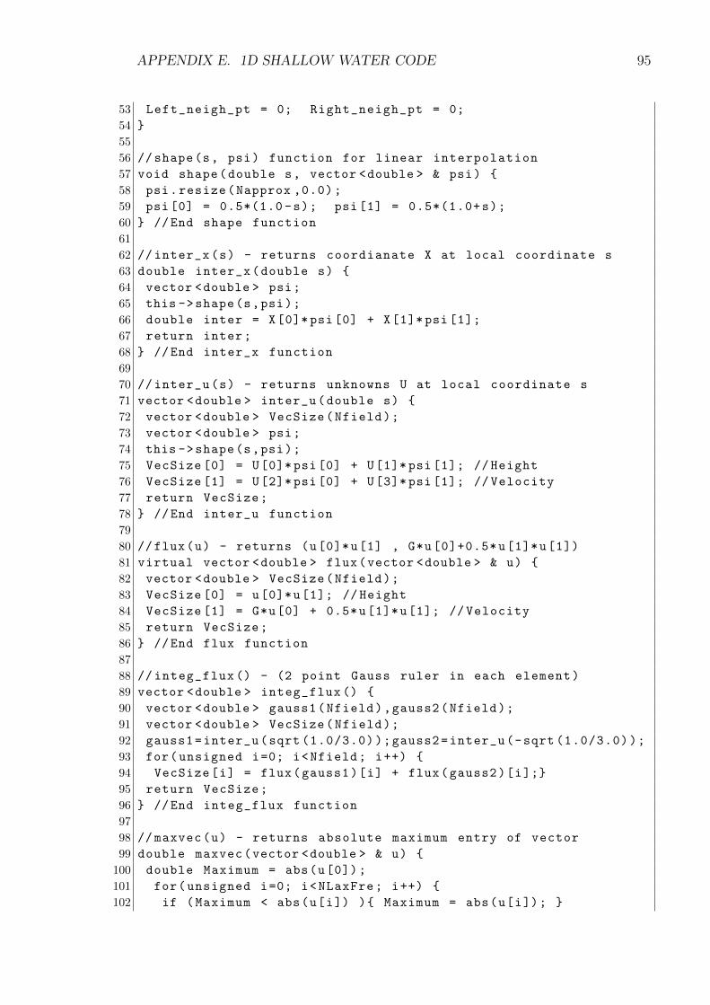
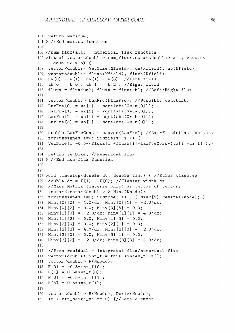
A complete, original C++ code to solve this problem, using linear approximation
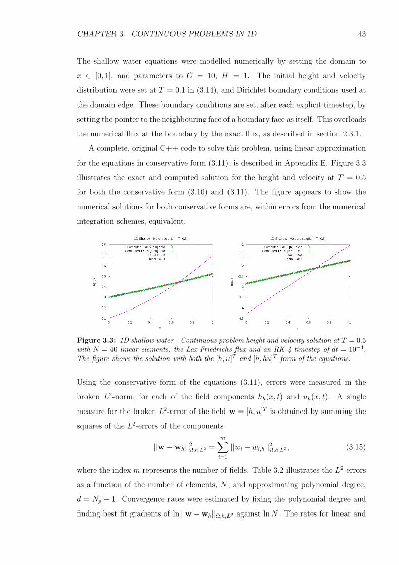
for the equations in conservative form (3.11), is described in Appendix E. Figure 3.3
illustrates the exact and computed solution for the height and velocity at T = 0.5
for both the conservative form (3.10) and (3.11). The figure appears to show the
numerical solutions for both conservative forms are, within errors from the numerical
integration schemes, equivalent.
Figure 3.3: 1D shallow water - Continuous problem height and velocity solution at T = 0.5with N = 40 linear elements, the Lax-Friedrichs flux and an RK-4 timestep of dt = 10−4.The figure shows the solution with both the [h, u]T and [h, hu]T form of the equations.
Using the conservative form of the equations (3.11), errors were measured in the
broken L2-norm, for each of the field components hh(x, t) and uh(x, t). A single
measure for the broken L2-error of the field w = [h, u]T is obtained by summing the
squares of the L2-errors of the components
||w −wh||2Ω,h,L2 =m∑i=1
||wi − wi,h||2Ω,h,L2 , (3.15)
where the index m represents the number of fields. Table 3.2 illustrates the L2-errors
as a function of the number of elements, N , and approximating polynomial degree,
d = Np − 1. Convergence rates were estimated by fixing the polynomial degree and
finding best fit gradients of ln ||w −wh||Ω,h,L2 against lnN . The rates for linear and
CHAPTER 3. CONTINUOUS PROBLEMS IN 1D 44
N d = 1 d = 2 d = 310 2.23× 10⁻³ 9.70× 10⁻⁴ 4.91× 10⁻¹⁴
20 5.24× 10⁻⁴ 2.18× 10⁻⁴ 4.93× 10⁻¹⁴
40 8.97× 10⁻⁵ 4.62× 10⁻⁵ 4.86× 10⁻¹⁴
80 1.88× 10⁻⁵ 9.69× 10⁻⁶ 3.25× 10⁻¹³
Rate 2.33 2.22 N/A
Table 3.2: 1D shallow water - Broken L2-errors for continuous problem at T = 0.5, withan RK-4 timestep of dt = 10−4 and a Lax-Friedrichs flux. The conserved field [h, u]T is usedand the errors are shown as a function of the number of elements, N , and the polynomialorder, d = Np − 1. The columns and rows represent h- and p-refinement respectively.
quadratic approximation were found to be 2.33 and 2.22 respectively, so increasing
the polynomial order did not increase the convergence rate. As discussed in section
2.8.1, error analysis for non-linear problems is difficult to achieve, but the solutions
are converging when performing h-refinement.
Figure 3.4: 1D shallow water - Continuous problem broken L2-errors at T = 0.5, with anRK-4 timestep of dt = 10−4 and a Lax-Friedrichs flux with the conserved field [h, u]T . Thelines represent h-refinement for fixed polynomial degrees 1 and 2 respectively.
Using a cubic approximation, the errors have dramatically decreased to O(10−13).
This is explained by considering the numerical flux matrix (2.17) and flux matrix
(2.16), evaluated at each explicit Euler timestep, in turn:
• Numerical Flux Matrix - For a continuous problem the field jumps between
boundaries are 0 and so the coefficients of the numerical flux matrix are an
evaluation of the flux at an element’s edge. The exact height and velocity are
quadratic and linear, so at cubic approximation the flux is evaluated exactly
CHAPTER 3. CONTINUOUS PROBLEMS IN 1D 45
and hence the numerical flux matrix coefficients are evaluated exactly.
• Flux Matrix - The flux matrix has a highest order term, uhdψdx
, that must
be integrated across each element. At cubic approximation, ∂ψ∂x
is a degree 2
polynomial and the exact solutions of u and h are degree 1 and 2 polynomials.
Thus the highest order flux term represents a polynomial of degree 5. At
cubic approximation, the GLL quadrature scheme has Nk = 4 knot points
and integrates degree 2Nk − 3 = 5 polynomials exactly.
The flux and numerical flux matrices are calculated exactly at each timestep, and the
errors of magnitude 10−13 are due to timestepping errors of the RK-4 scheme and the
finite machine precision.
It was also worth noting how a different flux affects the accuracy of the numer-
ical solution. Figure 3.5 displays the numerical solutions at T = 0.4 with linear
approximation obtained with the central (2.6) and Lax-Friedrichs (2.7) flux. At lin-
ear approximation, the central flux is clearly inferior to the Lax-Friedrichs flux, with
large discontinuities in the approximate solution present.
Figure 3.5: 1D shallow water - Central and Lax-Friedrichs flux comparison at T = 0.4swith an RK-4 timestep of dt = 10−4 and 40 linear elements.
Chapter 4
Discontinuous Problems in 1D
4.1 Inviscid Burgers’ equation
The 1D inviscid Burgers’ equation is an example of a 1D flux transport equation,
with non-linear flux f(w) = 12w2, leading to the PDE
∂w
∂t+
1
2
∂w2
∂x=∂w
∂t+ w
∂w
∂x= 0 x ∈ [A,B]. (4.1)
The PDE is useful to understand some of the basic theory behind shocks. In particu-
lar, shock formation, where a solution becomes multivalued at a single spatial point,
from continuous initial conditions, and shock propagation, where a discontinuous ini-
tial condition propagates through time.
4.1.1 Shock Formation
We revisit the the 1D kinematic wave equation
∂w
∂t+ c(w)
∂w
∂x= 0 x ∈ [A,B]. (4.2)
As described in section 3.1, exact solutions can be found using the method of charac-
teristics. The solution at a point (x, t) is given by w(x, t) = w(η, 0) where η is found
implicitly through x − η = c(w0(η))t. However, from theorem 3.1.1, for some initial
conditions unique solutions to the kinematic wave equation can not be guaranteed
for all time and a shock can develop in finite time.
Consider the kinematic wave equation (4.2), and find the total time derivative of
wx(x(t), t), the gradient of w along the characteristic x = x(t). Using the chain rule
46
CHAPTER 4. DISCONTINUOUS PROBLEMS IN 1D 47
and dxdt
= c(w) along a characteristic (3.3),
d
dtwx(x(t), t) = wtx +
dx
dtwxx = wtx + c(w)wxx.
Take the partial derivative with respect to x of the kinematic wave equation (4.2)
wtx + c(w)wxx +dc(w)
dww2x = 0,
and combining the above equations, leads to a first order differential equation,
d
dtwx = −c′(w)(wx)
2.
Using the boundary condition x = η at t = 0, and that w is constant on a character-
istic, the solution is
wx =w′0(η)
1 + w′0(η)c′(w0(η))t. (4.3)
For the inviscid Burgers’ equation (4.1), since c(w) = w is a strictly increasing func-
tion, then if the initial condition is not, the denominator of (4.3) will be equal to
zero in a finite time, the breaking time. The breaking point of the wave will thus be
on the characteristic in which the denominator first vanishes. Let
G(η) = c(w0(η)) =⇒ G′(η) = w′0(η)c′(w0(η)), (4.4)
the breaking point will be on the characteristic η = ηB, with the conditions that (i)
G′(ηB) < 0 and (ii) |G′(ηB)| is a maximum, with the time
TB = − 1
G′(ηB). (4.5)
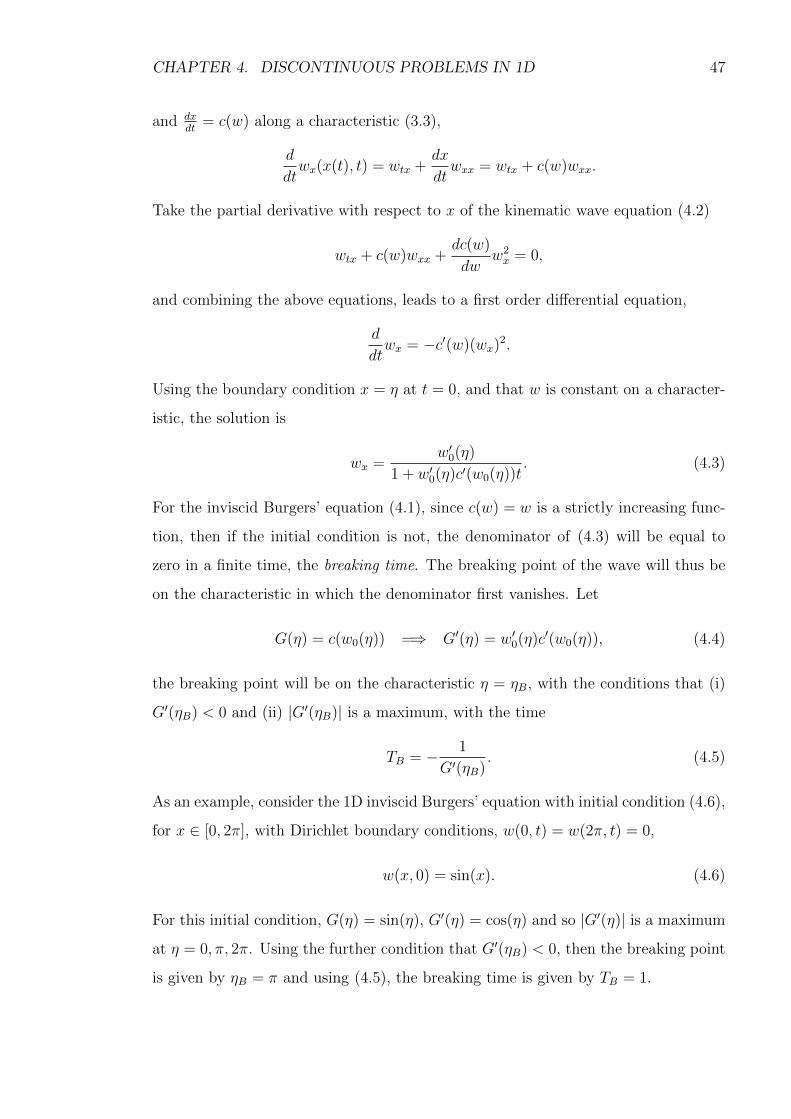
As an example, consider the 1D inviscid Burgers’ equation with initial condition (4.6),
for x ∈ [0, 2π], with Dirichlet boundary conditions, w(0, t) = w(2π, t) = 0,
w(x, 0) = sin(x). (4.6)
For this initial condition, G(η) = sin(η), G′(η) = cos(η) and so |G′(η)| is a maximum
at η = 0, π, 2π. Using the further condition that G′(ηB) < 0, then the breaking point
is given by ηB = π and using (4.5), the breaking time is given by TB = 1.
CHAPTER 4. DISCONTINUOUS PROBLEMS IN 1D 48
To model the inviscid Burgers’ equation numerically, the Lax-Friedrichs flux was
used. The Jacobian of the flux is w, and from the definition of the Lax-Friedrichs
flux (2.7)
CLF = maxwi,we
w, (4.7)
where wi and we are the internal and external fields at an element boundary. The
algorithm to compute the Lax-Friedrichs constant at an element edge can be seen
below and further details of the implementation can be seen in Appendix B.
1 Find wi and we
2 Compute Ci = wi, Ce = we
3 Take CLF = max(Ci, Ce)
Figure 4.1 represents the evolution of the numerical solution from T = 0 − 1.5,
at regular intervals of 0.5, with the sine wave initial condition and fixed boundary
conditions. As t → 1, the gradient of the solution at x = π becomes unbounded,
Figure 4.1: Burgers’ equation - Shock formation from smooth sinusoidal initial condition.An RK-4 timestep of dt = 5 × 10⁻⁴ is used with N = 400 linear elements and a Lax-Friedrichs flux. The left graphic illustrates the solution at regular time intervals of 0.5 andthe right graphic indicates that oscillations are removed with the MUSCL limiter.
and a shock develops. The approximation space, which is the space of linear func-
tions, is not adequate to deal with this discontinuity in the solution, resulting in the
oscillations of the solution near x = π at T = 1.5. In section 2.7, slope limiters
were constructed to remove such oscillations from a numerical solution. The MUSCL
slope limiter (2.35) was implemented, using the modified minmod function (2.39)
with smoothness parameter set to M = 5. The right hand graphic of figure 4.1 shows
the computed solution at T = 1.5 and the oscillatory behaviour has been removed.
CHAPTER 4. DISCONTINUOUS PROBLEMS IN 1D 49
4.1.2 Shock Propagation
As mentioned previously, another effect common in conservation laws is the effect
of shock propagation, in which a discontinuous initial condition propagates through
time. To understand this, we re-examine the integral form of a scalar conservation
law for a field, w, and flux, f , in one dimension (1.1),
d
dt
∫ R
L
w(x, t) dx = f(L, t)− f(R, t). (4.8)
It was shown in Section 1.1 that if w and f are continuously differentiable the familiar
PDE form for the conservation law can be recovered:
∂w
∂t+∂f
∂x= 0.
However, for a discontinuous initial condition, w0, the assumption that w is con-
tinuously differentiable is not true, and the method of characteristics to determine
solutions can not be directly used. Assume there is a smooth curve, x = s(t), in
which w has a simple discontinuity, so that w, and its derivatives, have well defined
limits as x→ s(t)− and x→ s(t)+ [1]. Consider the integral form (4.8)
d
dt
∫ s(t)
L
w(x, t) dx+d
dt
∫ R
s(t)
w(x, t) dx = f(L, t)− f(R, t),
with L < s(t) and R > s(t). Applying Leibniz’ rule [12, p.125], to evaluate the
derivative of an integral whose integrand and limits depend on the differentiation
where the following notation change has been used,
w±(t) = limx→s(t)±
w(x, t) and s′ =ds
dt.
Taking the limits L → s(t)−, R → s(t)+, the integral terms disappear, since w and
its derivatives are continuous away from the shock and (4.9) simplifies to the Rankine
Hugoniot condition
−s′[w] + [f(w)] = 0, (4.10)
CHAPTER 4. DISCONTINUOUS PROBLEMS IN 1D 50
where the curve s(t) is the shock path, and the propagating discontinuity in w is the
shock wave. The square bracket notation is the difference in the field across the dis-
continuity, [w] = w+(t)−w−(t). We write this shock condition as the correspondence
(...)t ↔ −s′[(...)], (...)x ↔ [(...)],
between a conservative PDE and its shock condition. Thus, for simple shocks, the
Rankine Hugoniot conditions determine not only the shock velocity, through (4.10),
but also the shock path, since s = x(t).
Consider the 1D inviscid Burgers’ equation, the shock velocity is given by
s′ =1
2
[w2]
[w]=
(w+(t)2 − w−(t)2)
2(w+(t)− w−(t))=w+(t) + w−(t)
2, (4.11)
the average value of w before and after the shock. For a general initial condition
this can be difficult to determine analytically, but consider the discontinuous initial
condition below, for x ∈ [−1, 1] = Ω, and Dirichlet boundary conditions w(−1, t) = 3
and w(1, t) = 1:
w(x, 0) =
3 if x < 0
1 if x > 0(4.12)
The initial condition (4.12) is piecewise constant and from (4.11) the shock speed is
s′ =3 + 1
2= 2. (4.13)
The shock moves with speed 2 in the positive x-direction. The characteristics are
straight lines either side of the shock, because the initial condition is piecewise con-
stant, and so the exact solution, for 0 < t < 0.5, is
w(x, t) = w(x− 2t, 0). (4.14)
Burgers’ equation was modelled with the above initial condition and Dirichlet bound-
ary conditions, w(−1, t) = 3 and w(1, t) = 1, consistent with the exact solution (4.14).
Figure 4.2 displays the solution at T = 0.25 without using a slope limiter. There
is oscillatory behaviour of the solution near the discontinuity and the behaviour for
h- and p-refinement is investigated. The left hand graphic of figure 4.3 displays the
solution with linear, quadratic and quartic approximation. Although using higher
order approximation appears to localise the oscillatory behaviour nearer to the shock
CHAPTER 4. DISCONTINUOUS PROBLEMS IN 1D 51
Figure 4.2: Burgers’ equation - Discontinuous solution with 160 linear elements at T =0.25 with an RK-4 timestep of dt = 10−4 and Lax-Friedrichs flux. The solution is exhibitingoscillatory behaviour near the shock.
region at x = 0.5, the oscillations are still clearly present. The number of elements
in the domain was also increased, with linear approximation. The right hand graphic
of figure 4.3 demonstrates that oscillatory behaviour is localised nearer to the shock
region, but again has not been removed.
Figure 4.3: Burgers’ equation - Discontinuous solutions with h- and p-refinement at T =0.25 without slope limiting. An RK-4 timestep of dt = 10−4 and Lax-Friedrichs flux wereused. The left hand figure represents N = 160 elements with linear, quadratic and quarticapproximation and the right hand figure is linear approximation with N = 80, 160 and 320elements for a domain x ∈ [−1, 1] and the figures show a zoom for x ∈ [0.4, 0.6].
Table 4.1 shows the broken L2-errors, at T = 0.25, as a function of the number
of elements, N , and polynomial degree, Np − 1. For this particular problem, the
errors are decreasing when performing h- and p-refinement. However, convergence is
slow, and using high order approximation has no effect on the convergence rate. It
CHAPTER 4. DISCONTINUOUS PROBLEMS IN 1D 52
remains a priority to remove the oscillatory behaviour present in figure 4.3 as this
could represent non-physical fluctuations in the field. For example, if the physical
process was modelling temperature or pressure, it is fundamental that these fields
remain positive.
N d = 1 d = 2 d = 3 d = 420 2.33× 10⁻¹ 1.81× 10⁻¹ 1.26× 10⁻¹ 8.73× 10⁻²
40 1.66× 10⁻¹ 1.27× 10⁻¹ 8.89× 10⁻² 6.17× 10⁻²
80 1.19× 10⁻¹ 8.98× 10⁻² 6.28× 10⁻² 4.36× 10⁻²
160 8.38× 10⁻² 6.35× 10⁻² 4.44× 10⁻² 3.08× 10⁻²
Rate 0.49 0.50 0.50 0.50
Table 4.1: Burgers’ equation - Discontinuous problem broken L2-errors as a function ofthe number of elements, N , and polynomial degree, d, at T = 0.25. An RK-4 timestep ofdt = 10−4 and the Lax-Friedrichs flux were used.
To remove the oscillations observed in figure 4.3, the MUSCL limiter, using the
modified minmod function, was applied to the numerical solution after each explicit
timestep of the RK-4 algorithm. Figure 4.4 represents the solution with the parameter
in the modified minmod function set to M = 0 and M = 5. Firstly, it can be seen
that the limiter does indeed do its job by removing the oscillations near the shock.
The errors are not sensitive to the parameter choice M , because this parameter was
designed to retain high order accuracy near regions of smooth extrema, as discussed
in section 2.7.5, which are not present in the exact solution (4.14).
Figure 4.5 displays the solution with linear, quadratic and quartic approximation.
The RK-4 timestepper and the RK-TVD3 timestepper were used to progress the
solution through time (see Appendix D for RK-TVD3 algorithm description). In both
cases the slope limiter is indeed removing the oscillatory behaviour for the different
polynomial orders. In section 2.7, the MUSCL limiter was shown to enforce each
explicit Euler timestep of the RK-TVD3 algorithm to be bounded in the TV semi-
norm (2.40). As a consequence, this gave us a bound on the growth of the numerical
solution in the total variation semi-norm in (2.28) leading to theorem 2.7.2. A similar
bound is not possible for the RK-4 timestepper, but the numerical results for both
timesteppers appear similar.
Table 4.2 shows the L2-errors with the MUSCL limiter, with M = 5, for the RK-4
and RK-TVD3 timestepper. It can be seen that the L2 errors are converging with
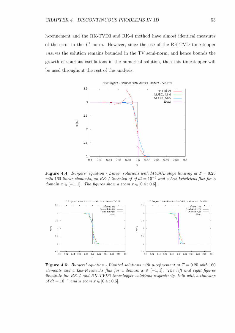
CHAPTER 4. DISCONTINUOUS PROBLEMS IN 1D 53
h-refinement and the RK-TVD3 and RK-4 method have almost identical measures
of the error in the L2 norm. However, since the use of the RK-TVD timestepper
ensures the solution remains bounded in the TV semi-norm, and hence bounds the
growth of spurious oscillations in the numerical solution, then this timestepper will
be used throughout the rest of the analysis.
Figure 4.4: Burgers’ equation - Linear solutions with MUSCL slope limiting at T = 0.25with 160 linear elements, an RK-4 timestep of of dt = 10−4 and a Lax-Friedrichs flux for adomain x ∈ [−1, 1]. The figures show a zoom x ∈ [0.4 : 0.6].
Figure 4.5: Burgers’ equation - Limited solutions with p-refinement at T = 0.25 with 160elements and a Lax-Friedrichs flux for a domain x ∈ [−1, 1]. The left and right figuresillustrate the RK-4 and RK-TVD3 timestepper solutions respectively, both with a timestepof dt = 10−4 and a zoom x ∈ [0.4 : 0.6].
CHAPTER 4. DISCONTINUOUS PROBLEMS IN 1D 54
N RKTVD3 RK420 3.32× 10⁻¹ 3.32× 10⁻¹
40 2.35× 10⁻¹ 2.35× 10⁻¹
80 1.67× 10⁻¹ 1.67× 10⁻¹
160 1.18× 10⁻¹ 1.18× 10⁻¹
Table 4.2: Burgers’ equation - Broken L2-errors with h-refinement and linear approxima-tion, with a Lax-Friedrichs flux. The RK-4 and RK-TVD3 timestepper are used to marchthe solution through time with MUSCL (M=5) slope limiting with a timestep of dt = 10−4.
4.2 Shallow water equations
We move onto a one dimensional discontinuous problem for the shallow water equa-
tions. In section 3.3 it was shown that these equations can be written in conservative
form, with field and flux
w =
h
hu
, f(w) =
hu
12Gh2 + u2h
, (4.15)
from which an alternative conservative form below was derived,
w =
h
u
, f(w) =
hu
Gh+ 12u2
, (4.16)
which were both used successfully to solve a continuous test problem for the shallow
water equations. In this chapter, we will discover that for a discontinuous problem
different numerical solutions are obtained, using the same initial conditions, for the
two different conservative forms. This result, which is not well documented in the
literature, is explained in section 4.2.4. To understand how exact solutions are de-
termined for discontinuous problems, it is essential to revisit the discussion on the
Rankine Hugoniot conditions for shock propagation discussed in section 4.1.2.
4.2.1 Rankine Hugoniot conditions
In section 4.1.2, the integral form of a conserved PDE was considered and the velocity
of a simple discontinuity was determined from the Rankine Hugoniot conditions. The
conditions for a conserved vector field turn out to be very similar to that of a scalar
field, but, this time there is a shock condition for each component of the field. To
CHAPTER 4. DISCONTINUOUS PROBLEMS IN 1D 55
be more precise, assuming a simple shock, and a conserved field u ∈ Rm, with
corresponding flux f(u) ∈ Rm, the Rankine Hugoniot conditions [1, p.180] are
−dsdt
[ui] + [f(u)i] = 0 i = 1 : m.
For the shallow water system in conserved form (4.15), with the field [h, hu]T , the
following Rankine Hugoniot conditions thus hold at a discontinuity:
ds
dt=
[hu]
[h],
ds
dt=
[hu2 +Gh2/2]
[hu]. (4.17)
However, in the conserved form (4.16), with the field [h, u]T , the Rankine Hugoniot
conditions below hold at a discontinuity:
ds
dt=
[hu]
[h],
ds
dt=
[u2/2 +Gh]
[hu].
Physically, the conserved form of the equations with field, [h, hu]T , represents the
true conserved properties of the system, the conservation of fluid mass and so (4.17)
are the correct Rankine Hugoniot conditions to use at a discontinuity.
4.2.2 Characteristic Curves
In section 3.1 characteristic curves were explored for a scalar field in 1 spatial dimen-
sion. Along these curves the PDE reduced to a simple ODE, along which the solution
w(x, t) remained constant. For an extension to a system of PDEs, we consider the
conserved form (4.15) and write the shallow water PDEs as
ht + uhx + hux = 0,
ut +Ghx + uux = 0.
Taking a linear combination of the above equations
α1(ht + uhx + hux) + α2(ut +Ghx + uux) = 0,
and grouping the derivatives of h and u
α1
[ht +
(u+
Gα2
α1
)hx
]+ α2
[ut +
(u+
α1
α2
h)ux
]= 0. (4.18)
Consider the linear combination below, with α1 = 1,
α2
α1
= ±√h
G,
CHAPTER 4. DISCONTINUOUS PROBLEMS IN 1D 56
then (4.18) becomes,
ht + (u±√Gh)hx ±
√h
G[ut + (u±
√Gh)ux] = 0. (4.19)
If we define the characteristic curves, C±, as
dx
dt= u±
√Gh, (4.20)
then the PDE (4.19) reduces to a set of ODEs, defined on the characteristic curves
(4.20) giving the characteristic form:
dh
dt±√h
G
du
dt= 0 along
dx
dt= u±
√Gh. (4.21)
4.2.3 1D Dam-Break Setup
A 1D dam-break problem, where the domain is set to Ω = [−D,D], the constant
G = 10 with Dirichlet boundary conditions h(−D, t) = hL, h(D, t) = hR, hL ≥ hR,
and the initial condition
h(x, 0) =
hL if x < 0
hR if x > 0u(x, 0) = 0.0, (4.22)
is studied. We can imagine stationary water of height hL separated by a thin sheet
at x = 0 from stationary water of height hR. At t = 0, the sheet is removed and,
ignoring the time to lift the sheet and any friction, the higher fluid, in the region
x < 0, travels into the region x > 0. The initial distribution is illustrated in figure
4.6 below.
Figure 4.6: Initial height distribution for 1D dam-break problem, h = 1 for x < 0 andh = 0.12 for x > 0.
CHAPTER 4. DISCONTINUOUS PROBLEMS IN 1D 57
Huang et al. [16] use the Rankine Hugoniot conditions (4.17) at the shock and
the characteristic curves (4.21) away from the shock, to find an exact solution that is
determined from the solution of a non-linear problem. This makes the 1D dam-break
problem ideal to understand how different numerical fluxes and the MUSCL slope
limiter effect the accuracy of the computed solution.
For the specific initial condition hL = 1, hR = 0.12, there are a number of key
features of the solution at time t as a function of the spatial coordinate x, as discussed
below:
• x < −√Gt - The water remains undisturbed, and the left hand initial condition,
h = 1, u = 0, is retained.
• −√Gt < x < 0.050
√Gt - At x = −
√Gt there is a discontinuity in the gradient,
the height decreases parabolically and the velocity increases linearly.
• 0.050√Gt < x < 0.977
√Gt - At x = 0.050
√Gt there is another discontinuity in
the gradient. This is the shock region and the height and velocity are constant,
hS = 0.423, uS = 0.699√G.
• x > 0.977√Gt - At x = 0.977
√Gt, there is a genuine discontinuity in the
height and velocity. After this point, the water remains undisturbed and the
right hand initial condition, h = 0.12, u = 0, is retained.
Figure 4.7: 1D dam-break - Exact height solution at T = 0.4 with G = 10 and the initialcondition (4.22) with hL = 1, hR = 0.12. The discontinuities in the gradients, at x ≈ −1.27and x ≈ 0.06, the true discontinuity, at x ≈ 1.24, and the shock height, hs = 0.423, areillustrated.
CHAPTER 4. DISCONTINUOUS PROBLEMS IN 1D 58
The conservative form (4.15), with the field [h, hu]T , is used to solve the 1D dam-
break problem and the Lax-Friedrichs flux used as described in (3.12). Figure 4.8
demonstrates the height and momentum solution at T = 0.4, with linear approxima-
tion. There are two areas where oscillations have been introduced into the solution.
There are large oscillations at x ≈ 0.1, where the exact solution has a discontinuity
in the gradient, and also at x ≈ 1.2, where the exact solution has a shock.
Figure 4.8: 1D dam-break - Height and momentum solution with at T = 0.4 with 1200linear elements, a Lax-Friedrichs flux and an RK-TVD3 timestep of dt = 10−4. If nolimiting is applied oscillations appear in the solution near discontinuities.
To remove these oscillations, a limiter is applied after each explicit timestep of
the RK-TVD3 algorithm. The MUSCL limiter (2.35) was implemented, using the
modified minmod function (2.39) with the smoothness parameter set to M = 50, and
figure 4.9 demonstrates the height solution, h. At the shock, x ≈ 1.23, the oscillations
have been removed by the MUSCL slope limiter. The solution has been plotted with
5 plot points per element, and so the shock is resolved in approximately 4 elements.
At the gradient discontinuity the MUSCL limiter is removing most of the oscillatory
behaviour, but has not resolved the solution as well as at the shock.
4.2.4 Importance of shocks and conserved forms
The conserved field [h, u]T and its associated flux in equation (4.16), derived in section
3.3, were now used to model the dam-break problem with the Lax-Freidrichs flux.
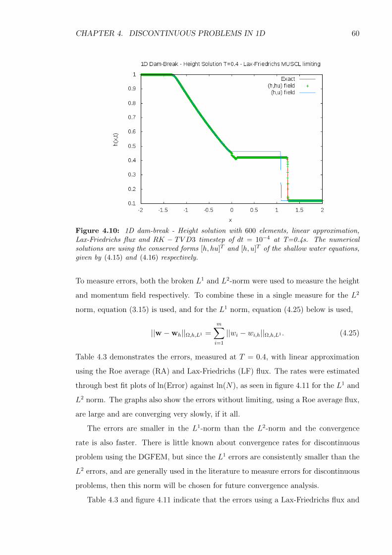
Figure 4.10 demonstrates the height solution, at T = 0.4, for both the conserved
fields [h, u]T and [h, hu]T . The figure clearly shows that if the conserved field [h, u]T
is used, the numerical solution is not a good approximation to the analytic solution
and is breaking early, at the same spatial resolution. The conserved PDEs with the
CHAPTER 4. DISCONTINUOUS PROBLEMS IN 1D 59
Figure 4.9: 1D dam-break - Height solution with 1200 elements, linear approximation, aLax-Friedrichs flux and RK-TVD3 timestep of dt = 10−4 with the domain x ∈ [−2, 2]. Theleft hand and right hand figures represent a zoom for x ∈ [−0.3 : 0.3] and x ∈ [1.22 : 1.25]respectively. The true discontinuity is being resolved in approximately 4 elements and theoscillations of the solution near the gradient discontinuity are nearly removed.
field [h, u]T were derived directly from the conserved form (4.15). However, these
two forms have different Rankine Hugoniot conditions at the shock, as discussed in
section 4.2.1, yielding different shock velocities. The conserved field [h, hu]T repre-
sents the true conserved properties of the system, the conservation of fluid mass and
linear momentum, and the conserved field [h, u]T yields alternative, but non-physical
solutions. It is thus fundamental to enforce the conservation of the correct physical
variables, height and momentum, for solutions with shocks. The correct conserved
form (4.15), with field [h, hu]T will be used throughout the rest of this chapter.
The Roe average flux, described in section 2.2.3, can also be used to pass information
between elements. This requires the evaluation of a new flux constant, CRA, at
each element edge. Consider the internal and external fields at a boundary: we =
[he, (hu)e]T and we = [he, (hu)e]
T . The constant is evaluated as:
CRA = maxh,u|u±√gh|, (4.23)
h =hi + he
2, u =
√hiui +
√heue√
hi +√he
. (4.24)
The algorithm to compute the Roe average constant at an element edge can be seen
below and further details of the implementation can be seen in Appendix B.
1 Find wi and we
2 Compute h = hi+he2 , u =
√uihi+
√uehe√
ui+√ue
, C− = |u−√Gh|, C+ = |u +
√Gh|
3 Take CRA = max(C−, C+)
CHAPTER 4. DISCONTINUOUS PROBLEMS IN 1D 60
Figure 4.10: 1D dam-break - Height solution with 600 elements, linear approximation,Lax-Friedrichs flux and RK − TV D3 timestep of dt = 10−4 at T=0.4s. The numericalsolutions are using the conserved forms [h, hu]T and [h, u]T of the shallow water equations,given by (4.15) and (4.16) respectively.
To measure errors, both the broken L1 and L2-norm were used to measure the height
and momentum field respectively. To combine these in a single measure for the L2
norm, equation (3.15) is used, and for the L1 norm, equation (4.25) below is used,
||w −wh||Ω,h,L1 =m∑i=1
||wi − wi,h||Ω,h,L1 . (4.25)
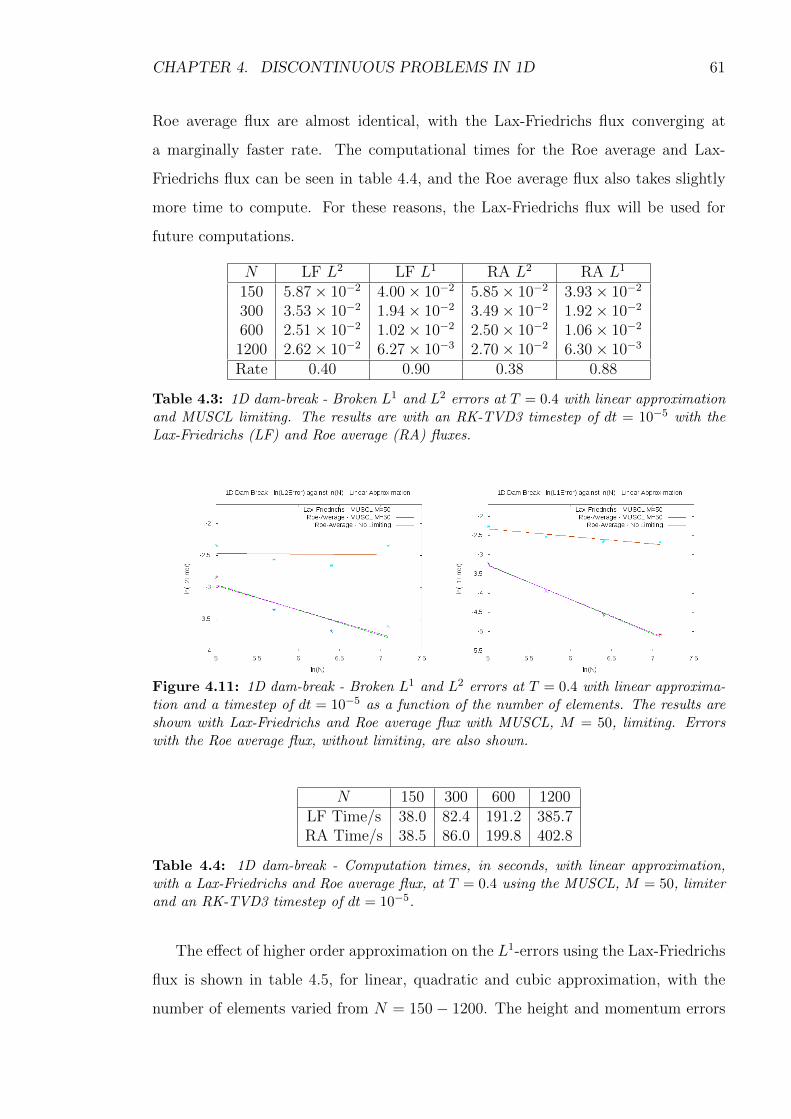
Table 4.3 demonstrates the errors, measured at T = 0.4, with linear approximation
using the Roe average (RA) and Lax-Friedrichs (LF) flux. The rates were estimated
through best fit plots of ln(Error) against ln(N), as seen in figure 4.11 for the L1 and
L2 norm. The graphs also show the errors without limiting, using a Roe average flux,
are large and are converging very slowly, if it all.
The errors are smaller in the L1-norm than the L2-norm and the convergence
rate is also faster. There is little known about convergence rates for discontinuous
problem using the DGFEM, but since the L1 errors are consistently smaller than the
L2 errors, and are generally used in the literature to measure errors for discontinuous
problems, then this norm will be chosen for future convergence analysis.
Table 4.3 and figure 4.11 indicate that the errors using a Lax-Friedrichs flux and
CHAPTER 4. DISCONTINUOUS PROBLEMS IN 1D 61
Roe average flux are almost identical, with the Lax-Friedrichs flux converging at
a marginally faster rate. The computational times for the Roe average and Lax-
Friedrichs flux can be seen in table 4.4, and the Roe average flux also takes slightly
more time to compute. For these reasons, the Lax-Friedrichs flux will be used for
future computations.
N LF L2 LF L1 RA L2 RA L1
150 5.87× 10⁻² 4.00× 10⁻² 5.85× 10⁻² 3.93× 10⁻²
300 3.53× 10⁻² 1.94× 10⁻² 3.49× 10⁻² 1.92× 10⁻²
600 2.51× 10⁻² 1.02× 10⁻² 2.50× 10⁻² 1.06× 10⁻²
1200 2.62× 10⁻² 6.27× 10⁻³ 2.70× 10⁻² 6.30× 10⁻³
Rate 0.40 0.90 0.38 0.88
Table 4.3: 1D dam-break - Broken L1 and L2 errors at T = 0.4 with linear approximationand MUSCL limiting. The results are with an RK-TVD3 timestep of dt = 10−5 with theLax-Friedrichs (LF) and Roe average (RA) fluxes.
Figure 4.11: 1D dam-break - Broken L1 and L2 errors at T = 0.4 with linear approxima-tion and a timestep of dt = 10−5 as a function of the number of elements. The results areshown with Lax-Friedrichs and Roe average flux with MUSCL, M = 50, limiting. Errorswith the Roe average flux, without limiting, are also shown.
Table 4.4: 1D dam-break - Computation times, in seconds, with linear approximation,with a Lax-Friedrichs and Roe average flux, at T = 0.4 using the MUSCL, M = 50, limiterand an RK-TVD3 timestep of dt = 10−5.
The effect of higher order approximation on the L1-errors using the Lax-Friedrichs
flux is shown in table 4.5, for linear, quadratic and cubic approximation, with the
number of elements varied from N = 150− 1200. The height and momentum errors
CHAPTER 4. DISCONTINUOUS PROBLEMS IN 1D 62
are combined using (4.25). Figure 4.12 represents h-refinement for the 1D dam-
break problem for different polynomial orders. For a fixed element size, increasing
the polynomial order does not reduce the error and similar convergence rates are
obtained for the different polynomial orders. The computation times are displayed
in table 4.6. Increasing the polynomial order increases the number of nodes in an
element, the mass matrix is larger, and so the timestepping algorithm (2.42) takes
longer to complete. These observations suggest that there is no advantage to be
gained from using higher order bases for the dam-break problem in the DGFEM.
N d = 1 d = 2 d = 3150 4.00× 10⁻² 3.94× 10⁻² 4.45× 10⁻²
300 1.94× 10⁻² 1.83× 10⁻² 2.57× 10⁻²
600 1.02× 10⁻² 1.04× 10⁻² 1.22× 10⁻²
1200 6.27× 10⁻³ 7.11× 10⁻³ 7.40× 10⁻³
Rate 0.90 0.82 0.88
Table 4.5: 1D dam-break - L1 errors, with N = 150 − 1200 elements, at T = 0.4 withlinear approximation and the MUSCL, M = 50, limiting. The results shown are usinglinear, quadratic and cubic approximation.
Figure 4.12: 1D dam-break - Broken L1-errors for the Height and Momentum solutionwith MUSCL, M = 50, limiter, Lax-Friedrichs Flux and RK-TVD3 timestep of dt = 10−5.The results shown are with linear, quadratic and cubic approximation.
N d = 1 d = 2 d = 3150 38.0 47.5 61.4300 82.4 107.8 141.8600 191.2 261.8 300.61200 385.7 690.0 814.2
Table 4.6: 1D dam-break - Computation times, in seconds, with a Lax-Friedrichs flux andRK-TVD3 timestep of dt = 10−5, for N = 150− 1200 elements, with linear, quadratic andcubic approximation.
CHAPTER 4. DISCONTINUOUS PROBLEMS IN 1D 63
4.2.5 Field Conservation
Consider the PDEs (4.15) and integrate each of the conserved fields over the domain,∫ 2
−2
(∂h∂t
+∂hu
∂x
)dx = 0 =⇒ d
dt
∫ 2
−2
hdx+ [hu]2−2 = 0,∫ 2
−2
(∂hu∂t
+∂(1
2Gh2 + u2h)
∂x
)dx = 0 =⇒ d
dt
∫ 2
−2
hudx+ [u2h+1
2Gh2]2−2 = 0,
=⇒ d
dt
∫ 2
−2
hdx = 0,d
dt
∫ 2
−2
hudx− 4.928 = 0.
For small times, the dam-break does not reach the boundary, and the field remains
unchanged, so that h(−2) = 1, h(2) = 0.12, u(−2) = u(2) = 0, which are also
enforced by the Dirichlet boundary conditions. The integral of the height field, h,
should stay constant, and the momentum field, hu, depend linearly on time. From
the initial condition,∫ 2
−2
h(x, 0)dx =
∫ 0
−2
1dx+
∫ 2
0
0.12dx = 2.24,∫ 2
−2
hu(x, 0)dx =
∫ 2
−2
0dx = 0.
So, for small enough times, the integrals should satisfy,∫ 2
−2
h(x, t)dx = 2.24,
∫ 2
2
hu(x, t)dx = 4.928t. (4.26)
Table 4.7 illustrates the integral average of the fields, with linear approximation at
times T = 0 − 0.4. It can be seen that the height field, h, remains unchanged, and
the momentum field, hu, is linearly increasing in time. The results are in excellent
Table 4.7: 1D dam-break - The integral of the height and momentum field across thedomain, measured in the broken L1-norm, as a function of the integration time, T. TheLax-Friedrichs flux, an RK-TVD3 timestep of dt = 10−4 with N = 1200 equally spacedlinear elements are used.
Chapter 5
2D Dam-Break Problem
5.1 Shallow water equations
For a domain Ω ⊂ R2, the shallow water equations model water waves under the
condition that a horizontal length scale is much larger than a vertical length scale
i.e. waves that have a wavelength much greater than the water depth. The equations
can be derived by considering fluid mass and momentum conservation in a control
volume of fluid [17].
The fluid is assumed to be of constant density, ρ, and any frictional, viscous or
Coriolis forces are ignored. The topographic height is also set constant, so the fluid
flows on a flat surface and hydrostatic equilibrium is assumed in the vertical direction.
These assumptions imply the velocity of the fluid is constant at a given point x in the
domain, so there is no variation with the fluid height. Defining the height, h(x, t),
and the velocities u(x, t) and v(x, t) in the x and y direction respectively, the shallow
water equations can be written,
∂
∂t(h) +
∂
∂x(hu) +
∂
∂x(hv) = 0,
∂
∂t(hu) +
∂
∂x(u2h+
1
2Gh2) +
∂
∂y(uvh) = 0,
∂
∂t(hv) +
∂
∂x(uvh) +
∂
∂y(v2h+
1
2Gh2) = 0,
and in conservative form (2.1), by defining the conserved field w = (h, hu, hv)T ∈ R3
64
CHAPTER 5. 2D DAM-BREAK PROBLEM 65
and the flux matrix F ∈ R3×2
F =
uh vh
u2h+ 12Gh2 uvh
uvh v2h+ 12Gh2
. (5.1)
As discussed in a 1D specialisation of these equations in section 4.2, these equations
pose a challenge numerically because solutions can have discontinuities present.
5.2 Discontinuous Galerkin Method in 2D
A discontinuous Galerkin method in 2D, with rectangular finite elements, is more
complex than in a single spatial dimension, for the following reasons:
• Neighbouring Scheme - An element in the mesh now has four neighbours, as
opposed to two neighbours in one spatial dimension and the elemental linear
system (2.18) requires coupling between adjacent faces in the mesh, as discussed
in section 2.3.1.
• Numerical Flux matrix- The contributions to this matrix are line integrals of the
numerical flux along the edge of the 2D element, instead of function evaluations
at the edge points of an element in one spatial dimension. The numerical
integration scheme was discussed in section 2.4.
• Mass and Flux matrix - The contributions to these matrices are 2D surface
integrals over the element, instead of line integrals across the element in one
spatial dimension. The numerical integration scheme was also discussed in
section 2.4.
• Slope Limiting - The process of slope limiting, to remove spurious oscillations
appearing in numerical solutions, needs to be addressed. This will be discussed
in the following section for rectangular finite elements aligned with the coordi-
nate axes.
CHAPTER 5. 2D DAM-BREAK PROBLEM 66
5.2.1 2D Slope Limiting
In section 2.7, slope limiting was introduced in the context of 1D problems. For the
MUSCL slope limiter, a TVBM property for the solution, where the solution remains
bounded in the TV semi-norm, was obtained by considering values of the field at
element edges in 1D grids (see theorem 2.7.2).
From the literature, it appears that a rigorous proof of 2D stability remains largely
unknown for general meshes. In this analysis a 2D limiter will be implemented that
will operate on piecewise bilinear approximation, of the form w = (a + bx)(c + dy),
in each element.
A slope limiter essentially attempts to remove spurious oscillations from the ap-
proximate solution by suitably replacing the approximate solution gradient in each
element. However, since a bilinear approximation has a twist term, Cxy, then a
single measure for the x and y gradient across an element does not exist, making the
limiting process less intuitive.
A rectangular domain will be considered, aligned with the coordinate axes. Con-
sider a rectangular element [xi, xi+1]×[yj, yj+1], where i, j are indices for the elements
in the x and y direction. After each explicit Euler timestep, before the limiter is im-
plemented, the approximate solution in element (i, j) will be converted from bilinear
to pure linear approximation of the form
w(x, t) = wi,j(t) + wx(t)(x− xi+1/2
∆xi/2
)+ wy(t)
(y − yj+1/2
∆yj/2
), (5.2)
where wx(t), wy(t) are the average gradients in the x and y direction and wi,j(t) is
the integral average of the field in element (i, j),
wi,j(t) =
∫ xi+1
xi
∫ yj+1
yj(a+ bx)(c+ dy)dxdy
∆xi∆yj.
This integral average over the element, is the field at the central point (xi+1/2, yj+1/2)
of the element, as the argument below shows:
wi,j(t) =
∫ xi+1
xi(a+ bx)dx
∫ yj+1
yj(c+ dy)dy
∆xi∆yj
=∆xi(a+ b/2(xi+1 + xi))∆yj(c+ d/2(yj+1 + yj)
∆xi∆yj
=(a+ b
(xi+1 + xi)
2
)(c+ d
(yj+1 + yj)
2
)= wi+1/2,j+1/2.
CHAPTER 5. 2D DAM-BREAK PROBLEM 67
The choice for the average gradients wx(t), wy(t) is not unique and in the implemen-
tation the conversion to pure linear approximation is achieved through the following
algorithm, for each field component:
• Find the approximate solution at the four corner (nodal) points of the element:
wi,j, wi+1,j, wi,j+1, wi+1,j+1.
• Find the gradients along bottom, top, left and right edge of element:
wx(t)Bottom =wi+1,j − wi,j
∆xiwx(t)Top =
wi+1,j+1 − wi,j+1
∆xi
wx(t)Left =wi,j+1 − wi,j
∆yjwx(t)Right =
wi+1,j+1 − wi+1,j
∆yj(5.3)
• Take arithmetic averages of quantities to find the gradients:
wx(t) =wx(t)Bottom + wx(t)Top
2wy(t) =
wy(t)Left + wy(t)Right2
(5.4)
wi,j wi+1,j
wi+1,j+1wi,j+1
wi,j∆yj
∆xi
wy,Left wy,Right
wx,Bottom
wx,Top
Figure 5.1: A rectangular element illustrating the data required to perform 2D limiting onbilinear approximation. The figure illustrates the approximate solution at the four nodes,the element widths, the approximate gradients given by (5.3) and the element average (atthe central point).
After the true bilinear approximation has been converted to linear approximation of
the form (5.2), without a twist term, the limiting process is similar to the 1D case.
A variant of the original 1D modified minmod function (2.39) is used,
m(a1, a2, a3) =
a1 if |a1| ≤M∆h2
m(a1, a2, a3) otherwise.(5.5)
CHAPTER 5. 2D DAM-BREAK PROBLEM 68
The x and y directions are treated independently, and in each element, for each field,
wx(t) and wy(t) are limited separately using the 2D modified minmod function (5.5).
Consider the x direction, the gradient wx(t) is replaced, using the 2D modified
minmod function (5.5) with h = ∆xi, to
w′
x(t) = m(wx(t),
wi+1,j(t)− wi,j(t)∆xi
,wi,j(t)− wi−1,j(t)
∆xi
), (5.6)
where wi,j is the average in element (i, j) and wi+1,j and wi−1,j are the averages in
elements (i+ 1, j) and (i− 1, j), the west and east neighbours.
Similarly for the y direction, the gradient wy(t) is replaced using the modified
minmod function (5.5), with h = ∆yj, to
w′
y(t) = m(wy(t),
wi,j+1(t)− wi,j(t)∆yj
,wi,j(t)− wi,j−1(t)
∆yj
), (5.7)
where wi,j+1 and wi,j−1 are the averages in elements (i, j+ 1) and (i, j−1), the north
and south neighbours.
To ensure conservation of the field, the average value, w(t), is forced to remain
invariant by the limiting process. This average value, for linear approximation, is the
field at the central point of the element and so the new unknowns, at the four nodal
positions, are reconstructed through the following formulae:
wi,j = wi,j(t)−∆xiw′
x/2−∆yjw′
y/2,
wi+1,j = wi,j(t) + ∆xiw′
x/2−∆yjw′
y/2,
wi,j+1 = wi,j(t)−∆xiw′
x/2 + ∆yjw′
y/2,
wi+1,j+1 = wi,j(t) + ∆xiw′
x/2 + ∆yjw′
y/2. (5.8)
The implementation of this 2D slope limiter into the oomph-lib is explained in more
detail in Appendix C. This includes a discussion of the process to find an element’s
neighbour and the actual implementation of the algorithm above.
5.3 2D Dam-Break Problem
A discontinuous problem in 2D can now be implemented, that of a 2D dam-break.
The Lax-Friedrichs flux will be used, using the definition (2.7), to define numerical
fluxes at element edges. This requires maximising the eigenvalues of the Jacobian
CHAPTER 5. 2D DAM-BREAK PROBLEM 69
of the flux matrix in the direction of the outer unit normal at an element edge.
Letting the general outer unit normal be (nx, ny)T , it is shown in Appendix A that
where the variables u0 = h, u1 = u, u2 = v. For rectangular meshes, with outer unit
normals aligned with the x and y axes, the eigenvalues simplify to:
• n = ±(0, 1)T - Normal parallel to y-axis:
λ1 = ±u2 +√Gu0, λ2 = ±u2, λ3 = ±u2 −
√Gu0.
• n = ±(1, 0)T - Normal parallel to x-axis:
λ1 = ±u1 +√Gu0, λ2 = ±u1, λ3 = ±u1 −
√Gu0.
In both cases the second eigenvalue can never be the largest in absolute value, and the
Lax-Friedrichs constant will be the maximum in absolute value of the first and third
eigenvalue across all possibilities of the field over the boundary. Assuming that this
maximum is taken only over the internal or external field, the resulting optimization
problem is almost identical to that of a 1D dam-break (3.13). The only difference
is what velocity to use in the optimization algorithm. If the outer unit normal is
parallel to y-axis, the y-velocity will be used in the optimization algorithm, and if
the outer unit normal is parallel to the x-velocity, the x-velocity will be used in the
optimization algorithm. See Appendix B for further details of the Numerical Flux
implementation.
5.3.1 Smoothed 2D Dam-Break Problem
For the smoothed 2D dam-break problem, the domain is set to (x, y) ∈ [−1, 1] ×
[−1, 1], with the initial condition
h(x, y, 0) = 0.75− 0.25 tanh(200((x2 + y2)− 0.25)),
u(x, y, 0) =v(x, y, 0) = 0. (5.9)
This is clearly not a genuine discontinuity, since the tanh function is smooth. How-
ever, tanh(x) changes very rapidly about x = 0 from −1 to +1. If x2 + y2 < 0.25,
CHAPTER 5. 2D DAM-BREAK PROBLEM 70
h(x, y, 0) ≈ 1, and if x2 + y2 > 0.25, h(x, y, 0) ≈ 0.5. The nearly discontinuous initial
condition is illustrated in figure 5.2, where the height distribution is plotted as a
function of the x-coordinate over the entire mesh.
Figure 5.2: 2D dam-break - Initial height distribution plotted as a function of the x-coordinate. The initial condition (5.9) is strictly smooth, but the height changes rapidlynear the region x2 + y2 = 0.25, making the initial distribution close to a true discontinuity.
From the literature, it appears that no analytic exact solution exists to this initial
value problem and validation of the results was performed by comparing the results
with code written by Chris Johnson [18]. He uses a finite volume method, devised by
Jiang et al. [5], which used a piecewise constant approximation within each element
and a limiter, called MinMod1, to slope limit the solution after each explicit timestep
of the Runge-Kutta algorithm.
The dam-break problem was modelled using the Lax-Friedrichs flux, periodic
boundary conditions, and the slope limiter described in section 5.2.1, for a linear
approximation. Figure 5.3 illustrates the average height solution in each element, for
elements lying on the y-axis, for both a non-limited and MUSCL limited solution.
The plot shows that different height solutions are obtained with and without a slope
limiter, with the non-limited solution oscillating in the region x ∈ ±[0.35 : 0.70]. For
a 100 × 100 grid the oscillations were so severe that no computational results were
obtainable without a slope limiter at T = 0.4.
CHAPTER 5. 2D DAM-BREAK PROBLEM 71
Figure 5.3: 2D dam-break - Illustration of the DGFEM average height solution for thedam-break problem on a 50 × 50 grid with an RK-TVD3 timestep of dt = 0.01 and Lax-Friedrichs flux for elements lying on the y-axis. Oscillatory behaviour can be observed inthe numerical solution without slope limiting but disappear with the 2D slope limiter.
Figure 5.4 is an illustration of the height density for different resolutions of the
grid, by plotting the average height in each element over the domain. This illustration
shows that as the resolution is increased, the shock, at r =√x2 + y2 ≈ 0.73, is better
resolved and circular symmetry is generally preserved. However, in the 50× 50 plot,
the height density is slightly greater at a radial distance of r ≈ 0.5 in the x and y
direction than at the same radial distance in directions 45o to the coordinate axes,
indicating a potential asymmetry of the 2D slope limiter.
Figure 5.5 is a plot of the average heights along the line y = x for different
resolutions of the grid. It can be clearly seen that the shock at r ≈ 0.73 is better
resolved as the mesh resolution is increased.
The DGFEM 2D dam-break results and an axisymmetric dam-break problem,
obtained by Chris Johnson [18], are compared. The axisymmetric dam-break prob-
lem implicitly assumes circular symmetry so only the radial direction is considered
and solutions can be found at a high spatial resolution. Figure 5.6 illustrates the
axisymmetric solution using a high resolution 12800 element 1D grid. The density
plot is the axisymmetric solution mapped onto a 12800 × 12800 2D grid and a plot
CHAPTER 5. 2D DAM-BREAK PROBLEM 72
of the axisymmetric solution as a function of the radial distance, r, is also shown.
Figure 5.7 illustrates a series of height density plots of the difference between
the element average from the 2D dam-break DGFEM results and the high resolution
axisymmetric FVM solution. As the DGFEM resolution is increased, the difference
between the solutions appears to be diminishing in the smoother regions of the solu-
tion. The discontinuous Galerkin method is also resolving where the shock location
is, to a high degree of accuracy, as the spatial resolution is increased. However, near
the discontinuity, the differences in the solution are still large.
Results for the actual 2D dam-break problem using the finite volume method were
obtained from Chris Johnson [18]. A better understanding of the DGFEM accuracy
was obtained by plotting the average height solution at different cross sections through
the domain for the FVM and DGFEM solutions, solved at the same spatial resolution.
The average height solutions, along the x-axis, y-axis and the line y = x, are plotted
in figures 5.8, 5.9 and 5.10 respectively. These graphs illustrate that the FVM and
DGFEM are both resolving the shock in approximately 6 elements on a 400 × 400
grid.
A plot of average height solutions of the DGFEM along the x-axis, y-axis and the
line x = y is illustrated in figure 5.11 along with the high resolution axisymmetric
dam-break solution. Along the x and y-axis the average height solutions are identical
and are also very similar to the average height solution along the line y = x.
CHAPTER 5. 2D DAM-BREAK PROBLEM 73
x
y
Average Height DGFEM 50 x 50 Elements − MUSCL
−1 −0.5 0 0.5 1
−1
−0.8
−0.6
−0.4
−0.2
0
0.2
0.4
0.6
0.8
1 0.5
0.55
0.6
0.65
0.7
0.75
0.8
0.85
0.9
0.95
x
y
Average Height DGFEM 100 x 100 Elements − MUSCL
−1 −0.5 0 0.5 1
−1
−0.8
−0.6
−0.4
−0.2
0
0.2
0.4
0.6
0.8
1 0.5
0.55
0.6
0.65
0.7
0.75
0.8
0.85
0.9
0.95
x
y
Average Height DGFEM 200 x 200 Elements − MUSCL
−1 −0.5 0 0.5 1
−1
−0.8
−0.6
−0.4
−0.2
0
0.2
0.4
0.6
0.8
1 0.5
0.55
0.6
0.65
0.7
0.75
0.8
0.85
0.9
0.95
1
x
y
Average Height DGFEM 400 x 400 Elements − MUSCL
−1 −0.5 0 0.5 1
−1
−0.8
−0.6
−0.4
−0.2
0
0.2
0.4
0.6
0.8
1 0.5
0.55
0.6
0.65
0.7
0.75
0.8
0.85
0.9
0.95
1
Figure 5.4: 2D dam-break - Density plots of the average height field in each element,at T = 0.5, with a Lax-Friedrichs flux and the 2D slope limiter. The figures represent a50 × 50, 100 × 100, 200 × 200 and a 400 × 400 grid with RK-TVD3 timesteps of dt =0.01, 0.005, 0.0025, 0.00125 respectively. A shock at r =
√x2 + y2 ≈ 0.73 can be observed
in the plots.
Figure 5.5: 2D dam-break - Average height solution along the line y = x for h-refinement.The figures represent data from a 50×50, 100×100, 200×200 and a 400×400 grid with RK-TVD3 timesteps of dt = 0.01, 0.005, 0.0025, 0.00125 respectively. As the mesh resolution isincreased the shock at r ≈ 0.73 is better resolved.
CHAPTER 5. 2D DAM-BREAK PROBLEM 74
x
y
Average Height FVM Interpolated 12800 x 12800 Cells
−1 −0.5 0 0.5 1
−1
−0.8
−0.6
−0.4
−0.2
0
0.2
0.4
0.6
0.8
1 0.5
0.55
0.6
0.65
0.7
0.75
0.8
0.85
0.9
0.95
1
Figure 5.6: Axisymmetric dam-break - The left hand figure illustrates an axisymmetricdam-break problem solution, h(r, t), mapped into the (x, y) plane. The solution resolutionis on a 12800 element grid and is deemed a good approximation to the exact 2D dam-breakproblem solution. The right hand figure illustrates the height as a function of the radius,illustrating a shock at r ≈ 0.73.
x
y
Average Height Error DGFEM 50 x 50 Elements − MUSCL
−1 −0.5 0 0.5 1
−1
−0.8
−0.6
−0.4
−0.2
0
0.2
0.4
0.6
0.8
1−0.08
−0.06
−0.04
−0.02
0
0.02
0.04
0.06
0.08
x
y
Average Height Error DGFEM 100 x 100 Elements − MUSCL
−1 −0.5 0 0.5 1
−1
−0.8
−0.6
−0.4
−0.2
0
0.2
0.4
0.6
0.8
1
−0.08
−0.06
−0.04
−0.02
0
0.02
0.04
0.06
0.08
x
y
Average Height Error DGFEM 200 x 200 Elements − MUSCL
−1 −0.5 0 0.5 1
−1
−0.8
−0.6
−0.4
−0.2
0
0.2
0.4
0.6
0.8
1 −0.1
−0.08
−0.06
−0.04
−0.02
0
0.02
0.04
0.06
0.08
x
y
Average Height Error DGFEM 400 x 400 Elements − MUSCL
−1 −0.5 0 0.5 1
−1
−0.8
−0.6
−0.4
−0.2
0
0.2
0.4
0.6
0.8
1
−0.08
−0.06
−0.04
−0.02
0
0.02
0.04
0.06
0.08
Figure 5.7: 2D dam-break - Density plots of the difference in the average height in eachelement, at T = 0.5, between a finite volume method and discontinuous Galerkin method.The figures represent a 50× 50, 100× 100, 200× 200 and a 400× 400 grid with RK-TVD3timesteps of dt = 0.01, 0.005, 0.0025, 0.00125 respectively. The difference near the shockat r =
√x2 + y2 ≈ 0.73 is large, but the solutions are approximately the same in smooth
regions.
CHAPTER 5. 2D DAM-BREAK PROBLEM 75
Figure 5.8: 2D dam-break - Illustration of the average DGFEM height solution for the 2Ddam-break problem on a 400× 400 grid with an RK-TVD3 timestep of dt = 0.00125 alongthe x-axis. The comparison with the finite volume method shows that the two methods havevery similar shock resolutions, from the zoom of the solution x ∈ [0.70 : 0.76], although theDGFEM appears marginally sharper.
Figure 5.9: 2D Dam-Break - Illustration of the average DGFEM height solution for the2D dam-break problem on a 400 × 400 grid with an RK-TVD3 timestep of dt = 0.00125along the y-axis. The FVM and DGFEM again have very similar shock resolutions.
Figure 5.10: 2D Dam-Break - Illustration of the average DGFEM and FVM height solutionfor the 2D dam-break problem on a 400 × 400 grid with an RK-TVD3 timestep of dt =0.00125 along the line y = x. Again, the DGFEM and FVM have very similar resolutionsof the shock.
CHAPTER 5. 2D DAM-BREAK PROBLEM 76
Figure 5.11: 2D Dam-Break - Illustration of the average DGFEM height solution for the2D dam-break problem on a 400 × 400 grid with an RK-TVD3 timestep of dt = 0.00125along the y-axis, x-axis and line y = x. The figure represents a zoom of the solution withr ∈ [0.70 : 0.76]. The FVM axisymmetric high resolution solution is also shown. The threedirections show very similar solutions near the shock, as one would expect from a circularlysymmetric dam-break problem.
Chapter 6
Conclusion
A discontinuous Galerkin formulation for a system of conserved PDEs was derived,
with a discussion of different types of numerical flux that can be assigned at the edges
of adjacent elements. In 1D, an analysis of the total variation diminishing explicit
Runge-Kutta class of timesteppers was undertaken to enforce numerical solutions to
be bounded in the total variation semi-norm by using MUSCL slope limiting.
Exact solutions were found, using the method of characteristics, for the advec-
tion equation. Using the Lax-Friedrichs flux, L2-errors were computed for a smooth
problem and these agreed well with theoretical convergence bounds in this norm. A
continuous problem for the 1D shallow water equations was implemented and the
Lax-Friedrichs flux was a superior choice to the central flux.
A theoretical discussion of shock formation and propagation was carried out
relating to the 1D inviscid Burgers’ equation. Numerical simulations, using the
Lax-Friedrichs flux at element edges, without slope limiting displayed oscillatory be-
haviour for discontinuous problems. These oscillations were completely removed when
the MUSCL limiter was applied to the numerical solutions.
A discontinuous dam break problem of the shallow water equations was also solved
numerically with MUSCL slope limiting. The numerical solutions converged when
performing h-refinement at different polynomial orders. However, for a fixed element
size, higher order approximation did not decrease the broken L1-errors. This sug-
gested, for this particular problem, that there there is no advantage in using high
order bases in the DGFEM. However, convergence analysis in strictly smooth regions
77
CHAPTER 6. CONCLUSION 78
of the solutions was not undertaken. It also appeared that the Lax-Friedrichs flux
was marginally more accurate, and quicker, than the Roe average flux.
A different conserved form for the shallow water equations was derived and used
to compute solutions to a continuous problem and the dam-break problem. For the
continuous problem, the two forms of the equations led to equivalent results. However,
for the dam-break problem, one of the forms was converging to a non physical solution.
For problems with shocks, it is essential to enforce conservation of the correct physical
variables. So, for the shallow water equations, it is necessary to use a form of the
equations that describe the conservation of fluid mass and momentum.
In 2D, a slope limiter applicable to quadrilateral finite elements aligned with the
coordinate axes was implemented into the oomph-lib. This limiter operates by re-
placing an average solution gradient in the x and y directions separately, using the
modified minmod function. Numerical results for a 2D dam break problem were ob-
tained using the DGFEM, with a Lax-Friedrichs flux, and shocks were being resolved
when performing h-refinement. A comparison was made with results from a finite
volume method [18] and suggested that at the same spatial resolution both methods
were resolving the shock over the same length scale.
6.1 Further Work
In the current implementation, the method of finding neighbouring bulk elements
through the face elements in 2D slope limiting is inefficient and could be modified by
storing direct pointers to neighbouring bulk elements. The current execution time
could also be reduced by using variable timesteps. At each Runge-Kutta timestep,
the fastest wave speed in the system could be calculated over the mesh and this used
to find a timestep satisfying the CFL condition within a desired tolerance.
For the shallow water equations, a slope limiter for general quadrilateral elements
that are not aligned with the coordinate axes could also be devised so that problems
over irregular domains could be computed. Also, a modification of the governing
equations could be achieved to model flow other bumpy terrains so that more realistic
problems for shallow water flow could be investigated.
The 2D slope limiter was devised by essentially performing 1D MUSCL slope
CHAPTER 6. CONCLUSION 79
limiting in two orthogonal directions. The 1D MUSCL limiter ensured that numerical
solutions were total variation bounded at each explicit timestep and it would be
interesting to see if an analogous property could be found for the 2D slope limiter
developed in this report. It would also be of interest to construct slope limiter in 2D
that operate on pure bilinear and biquadratic approximation.
A further theoretical investigation could be carried out into the 1D shallow water
equations with the conserved field [h, u]T . An exact solution for this set of equations
could be obtained by using the Rankine Hugoniot conditions at the discontinuity.
It would be reassuring to see if the non physical solution obtained in the numerical
experiments agreed with such an analytic exact solution.
Appendix A
Shallow Water numerical flux
Lax-Friedrichs constant
In section 2.2 it was stated that the eigenvalues of the matrix B = n. ∂F∂w
must be
calculated to find the Lax-Friedrichs flux constant. In component form, this matrix
is given by
Bik =∂Fij∂wk
nj. (A.1)
Flux Jacobian
The Jacobian of the flux matrix is a rank-3 tensor
Jijk =∂Fij∂wk
so J ∈ RNf×Np×Nf , (A.2)
where the indices j = 0 : Np − 1, i, k = 0 : Nf − 1, run over the spatial dimensions
and fields repectively. The flux for the 2D shallow water equations (5.1) is
F =
uh vh
u2h+ 12Gh2 uvh
uvh v2h+ 12Gh2
,
and the unknown field is w = [h, hu, hv]T = [u0, u1, u2]T . It is convenient to introduce
the notation, u1 = u1/u0 and u2 = u2/u0. From the definition of the Jacobian (A.2)
80
APPENDIX A. SHALLOW WATER NUMERICAL FLUX 81
the 18 entries are computed as below:
J000 = 0.0 J001 = 1.0 J002 = 0.0
J010 = 0.0 J011 = 0.0 J012 = 1.0
J100 = −u21 +Gu0 J101 = 2u1 J102 = 0.0
J110 = −u1u2 J111 = u2 J112 = u1
J200 = −u1u2 J201 = u2 J202 = u1
J210 = −u22 +Gu0 J211 = 0.0 J212 = 2u2
Jacobian eigenvalues in normal direction
The definition of the matrix B (A.1) requires the contraction of the tensor above
with the outer unit normal n = (nx, ny)T at an element’s edge,
B =
0.0 nx ny
(−u21 +Gu0)nx − (u1u2)ny (2u1)nx + (u2)ny (u1)ny
−(u1u2)nx + (−u22 +Gu0)nx u2nx (u1)nx + (2u2)ny
.
From the solutions of the eigenvalue equation det(B − λI) = 0, the eigenvalues are: