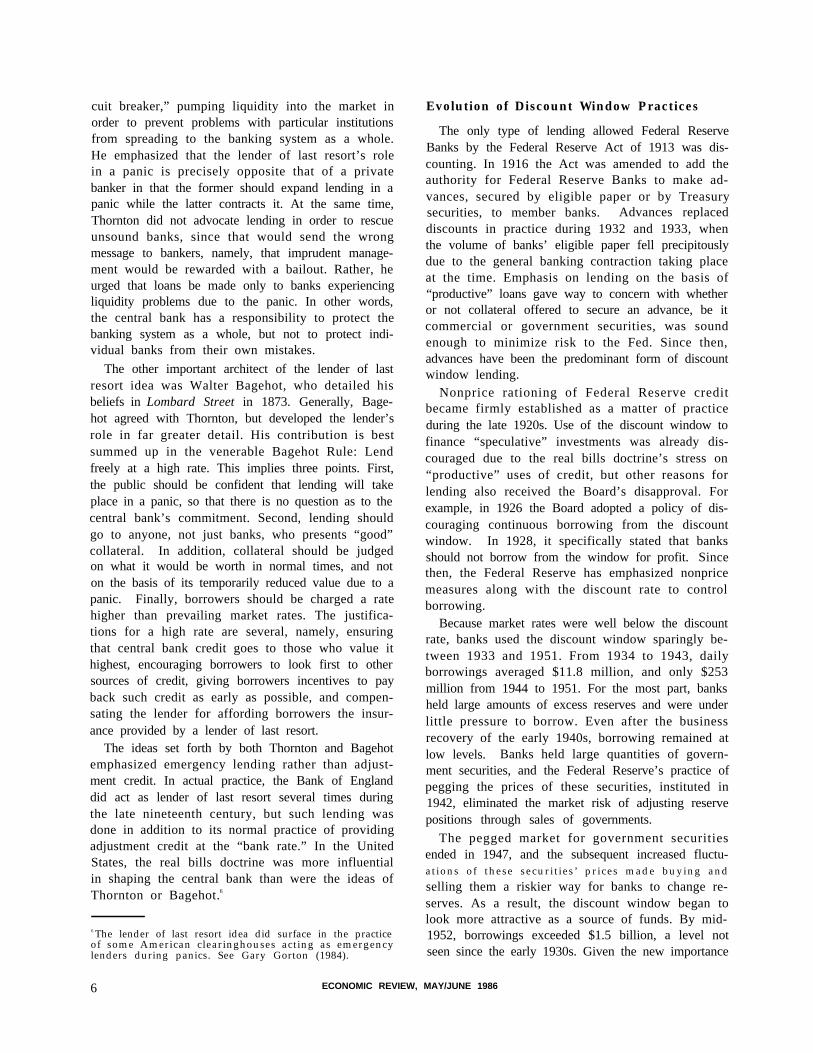
THE DISCOUNT -WINDOW - St. Louis Fed · rate on fed funds on this particular Wednesday afternoon...

THE DISCOUNT -WINDOWDavid L. Mengle

The discount window refers to lending by each ofthe twelve regional Federal Reserve Banks to deposi-tory institutions. Discount window loans generallyfund only a small part of bank reserves: For ex-ample, at the end of 1985 discount window loanswere less than three percent of total reserves. Never-theless, the window is perceived as an important toolboth for reserve adjustment and as part of currentFederal Reserve monetary control procedures.

Mechanics of a Discount Window Transaction

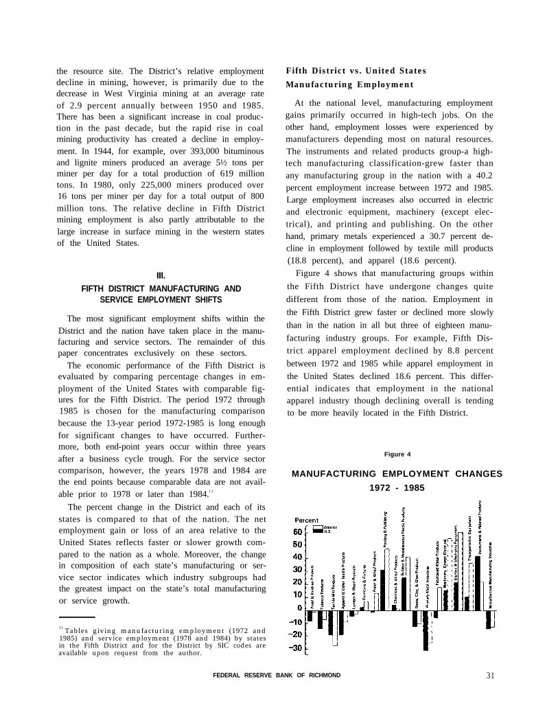
Discount window lending takes place through thereserve accounts depository institutions are requiredto maintain at their Federal Reserve Banks. In otherwords, banks borrow reserves at the discount win-dow. This is illustrated in balance sheet form inFigure 1. Suppose the funding officer at Ralph’sBank finds it has an unanticipated reserve deficiencyof $l,000,000 and decides to go to the discountwindow for an overnight loan in order to cover it.Once the loan is approved, the Ralph’s Bank reserveaccount is credited with $l,000,000. This shows upon the asset side of Ralph’s balance sheet as an in-crease in “Reserves with Federal Reserve Bank,”and on the liability side as an increase in “Borrow-ings from Federal Reserve Bank.” The transactionalso shows up on the Federal Reserve Bank’s balancesheet as an increase in “Discounts and Advances”on the asset side and an increase in “Bank Reserve

* An abbreviated version of this article will appear as achapter in Instruments of the Money Market, 6th edition,Federal Reserve Bank of Richmond, 1986 (forthcom-ing December 1986).

Accounts” on the liability side. This set of balancesheet entries takes place in all the examples given inthe Box.

The next day, Ralph’s Bank could raise the fundsto repay the loan by, for example, increasing depositsby $1,000,000 or by selling $l,000,000 of securities.In either case, the proceeds initially increase reserves.Actual repayment occurs when Ralph’s Bank’s re-serve account is debited for $l,000,000, which erasesthe corresponding entries on Ralph’s liability side andon the Reserve Bank’s asset side.

Discount window loans, which are granted to insti-tutions by their district Federal Reserve Banks, canbe either advances or discounts. Virtually all loanstoday are advances, meaning they are simply loanssecured by approved collateral and paid back withinterest at maturity. When the Federal ReserveSystem was established in 1914, however, the onlyloans authorized at the window were discounts, alsoknown as rediscounts. Discounts involve a borrowerselling “eligible paper,” such as a commercial oragricultural loan made by a bank to one of its cus-tomers, to its Federal Reserve Bank. In return, theborrower’s reserve account is credited for the dis-counted value of the paper. Upon repayment, theborrower gets the paper back, while its reserve ac-count is debited for the value of the paper. In thecase of either advances or discounts, the price ofborrowing is determined by the level of the discountrate prevailing at the time of the loan.

Although discount window borrowing was origi-nally limited to Federal Reserve System memberbanks, the Monetary Control Act of 1980 opened the

Figure 1

BORROWING FROM THE DISCOUNT WINDOW

ECONOMIC REVIEW, MAY/JUNE 1986

Examples of Discount Window Transactions

Example 1 - It is Wednesday afternoon at a regional bank, and the bank is required to haveenough funds in its reserve account at its Federal Reserve Bank to meet its reserve require-ment over the previous two weeks. The bank finds that it must borrow in order to make up itsreserve deficiency, but the money center (that is, the major New York, Chicago, and California)banks have apparently been borrowing heavily in the federal funds market. As a result, therate on fed funds on this particular Wednesday afternoon has soared far above its level earlierthat day. As far as the funding officer of the regional bank is concerned, the market for fundsat a price she considers acceptable has “dried up.” She calls the Federal Reserve Bank for adiscount window loan.

Example 2 - A West Coast regional bank, which generally avoids borrowing at the discount win-dow, expects to receive a wire transfer of $300 million from a New York bank, but by lateafternoon the money has not yet shown up. It turns out that the sending bank had due to anerror accidentally sent only $3,000 instead of the $300 million. Although the New York bank islegally liable for the correct amount, it is closed by the time the error is discovered. In orderto make up the deficiency in its reserve position, the West Coast bank calls the discount windowfor a loan.

Example 3 - It is Wednesday reserve account settlement at another bank, and the funding officernotes that the spread between the discount rate and fed funds rate has widened slightly. Sincehis bank is buying fed funds to make up a reserve deficiency, he decides to borrow part of thereserve deficiency from the discount window in order to take advantage of the spread. Over thenext few months, this repeats itself until the bank receives an “informational” call from the dis-count officer at the Federal Reserve Bank, inquiring as to the reason for the apparent pattern indiscount window borrowing. Taking the hint, the bank refrains from continuing the practiceon subsequent Wednesday settlements.

Exampl e 4 - A money center bank acts as a clearing agent for the government securities market.This means that the bank maintains book-entry securities accounts for market participants, andthat it also maintains a reserve account and a book-entry securities account at its Federal Re-serve Bank, so that securities transactions can be cleared through this system. One day, aninternal computer problem arises that allows the bank to accept securities but not to processthem for delivery to dealers, brokers, and other market participants. The bank’s reserve ac-count is debited for the amount of these securities, but it is unable to pass them on and collectpayment for them, resulting in a growing overdraft in the reserve account. As close of businessapproaches, it becomes increasingly clear that the problem will not be fixed in time to collectthe required payments from the securities buyers. In order to avoid a negative reserve balanceat the end of the day, the bank estimates its anticipated reserve account deficiency and goes tothe Federal Reserve Bank discount window for a loan for that amount. The computer problemis fixed and the loan is repaid the following day.

Exampl e 5 - Due to mismanagement, a privately insured savings and loan association fails. Outof concern about the condition of other privately insured thrift institutions in the state, deposi-tors begin to withdraw their deposits, leading to a run. Because they are not federally insured,some otherwise sound thrifts are not able to borrow from the Federal Home Loan Bank Boardin order to meet the demands of the depositors. As a result, the regional Federal Reserve Bankis called upon to lend to these thrifts. After an extensive examination of the collateral the thriftscould offer, the Reserve Bank makes loans to them until they are able to get federal insuranceand attract back enough deposits to pay back the discount window loans.

window to all depository institutions, except bankers’ Finally, subject to determination by the Board ofbanks, that maintain transaction accounts (such as Governors of the Federal Reserve System thatchecking and NOW accounts) or nonpersonal time “unusual and exigent circumstances” exist, discountdeposits. In addition, the Fed may lend to the United window loans may be made to individuals, partner-States branches and agencies of foreign banks if they ships, and corporations that are not depository insti-hold deposits against which reserves must be kept. tutions. Such lending would only take place if the

FEDERAL RESERVE BANK OF RICHMOND 3

Board and the Reserve Bank were to find that creditfrom other sources is not available and that failureto lend may have adverse effects on the economy.This last authority has not been used since the 1930s.

Discount window lending takes place under twomain programs, adjustment credit and extendedcredit.l Under normal circumstances adjustmentcredit, which consists of short-term loans extendedto cover temporary needs for funds, should accountfor the larger part of discount window credit. Loansto large banks under this program are generallyovernight loans, while small banks may take as longas two weeks to repay. Extended credit providesfunds to meet longer term requirements in one ofthree forms. First, seasonal credit can be extended tosmall institutions that depend on seasonal activitiessuch as farming or tourism, and that also lack readyaccess to national money markets. Second, extendedcredit can be granted to an institution facing specialdifficulties if it is believed that the circumstanceswarrant such aid. Finally, extended credit can go togroups of institutions facing deposit outflows due tochanges in the financial system, natural disasters, orother problems common to the group (see Box, Ex-ample 5). The second and third categories of ex-tended credit may involve a higher rate than thebasic discount rate as the term of borrowing growslonger.

In order to borrow from the discount window, thedirectors of a depository institution first must pass aborrowing resolution authorizing certain officers toborrow from their Federal Reserve Bank. Next, alending agreement is drawn up between the institu-tion and the Reserve Bank. These two preliminariesout of the way, the bank requests a discount windowloan by calling the discount officer of the ReserveBank and telling the amount desired, the reason forborrowing, and the collateral pledged against theloan. It is then up to the discount officer whetheror not to approve it.

Collateral, which consists of securities which couldbe sold by the Reserve Bank if the borrower fails topay back the loan, limits the Fed’s (and thereforethe taxpaying public’s) risk exposure. Acceptablecollateral includes, among other things, U. S. Trea-sury securities and government agency securities,municipal securities, mortgages on one-to-four family

1 For more detailed information on discount windowadministration policies, see Board of Governors of theFederal Reserve System, The Federal Reserve DiscountWindow (Board of Governors, 1980). The federal regu-lation governing the discount window is Regulation A,12 C.F.R. 201.

dwellings, and short-term commercial notes. Usually,collateral is kept at the Reserve Bank, although someReserve Banks allow institutions with adequate in-ternal controls to retain custody.

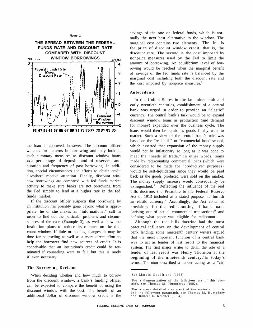
The discount rate is established by the Boards ofDirectors of the Federal Reserve Banks, subject toreview and final determination by the Board of Gov-ernors. If the discount rate were always set wellabove the prevailing fed funds rate, there would belittle incentive to borrow from the discount windowexcept in emergencies or if the funds rate for a par-ticular institution were well above that for the rest ofthe market. Since the 1960s, however, the discountrate has more often than not been set below the fundsrate. Figure 2, which portrays both adjustment creditborrowing levels and the spread between the tworates from 1955 to 1985, shows how borrowing tendsto rise when the rate spread rises.

The major nonprice tool for rationing discountwindow credit is the judgment of the Reserve Bankdiscount officer, whose job is to verify that lending ismade only for “appropriate” reasons. Appropriateuses of discount window credit include meeting de-mands for funds due to unexpected withdrawals ofdeposits, avoiding overdrafts in reserve accounts, andproviding liquidity in case of computer failures (seeBox, Example 4), natural disasters, and other forcesbeyond an institution’s control.2

An inappropriate use of the discount windowwould be borrowing to take advantage of a favorablespread between the fed funds rate and the discountrate (Example 3). Borrowing to fund a sudden,unexpected surge of demand for bank loans may beconsidered appropriate, but borrowing to fund adeliberate program of actively seeking to increaseloan volume would not. Continuous borrowing atthe window is inappropriate. Finally, an institutionthat is a net seller (lender) of federal funds shouldnot at the same time borrow at the window, norshould one that is conducting reverse repurchaseagreements (that is, buying securities) with the Fedfor its own account.

The discount officer’s judgment first comes intoplay when a borrower calls for a loan and states thereason. The monitoring does not end when (and if)

2 In order to encourage depository institutions to takemeasures to reduce the probability of operating problemscausing overdrafts, the Board of Governors announced inMay 1986 that a surcharge would be added to the dis-count rate for large borrowings caused by operatingproblems unless the problems are “clearly beyond thereasonable control of the institution.” See “Fed to Assess2-Point Penalty on Loans for Computer Snafus,” Ameri-can Banker, May 21, 1986.

4 ECONOMIC REVIEW, MAY/JUNE 1986

Figure 2

THE SPREAD BETWEEN THE FEDERALFUNDS RATE AND DISCOUNT RATE

COMPARED WITH DISCOUNTWINDOW BORROWINGS

the loan is approved, however. The discount officerwatches for patterns in borrowing and may look atsuch summary measures as discount window loansas a percentage of deposits and of reserves, andduration and frequency of past borrowing. In addi-tion, special circumstances and efforts to obtain creditelsewhere receive attention. Finally, discount win-dow borrowings are compared with fed funds marketactivity to make sure banks are not borrowing fromthe Fed simply to lend at a higher rate in the fedfunds market.

If the discount officer suspects that borrowing byan institution has possibly gone beyond what is appro-priate, he or she makes an “informational” call inorder to find out the particular problems and circum-stances of the case (Example 3), as well as how theinstitution plans to reduce its reliance on the dis-count window. If little or nothing changes, it may betime for counseling as well as a more direct effort tohelp the borrower find new sources of credit. It isconceivable that an institution’s credit could be ter-minated if counseling were to fail, but this is rarelyif ever necessary.

The Borrowing Decision

When deciding whether and how much to borrowfrom the discount window, a bank’s funding officercan be expected to compare the benefit of using thediscount window with the cost. The benefit of anadditional dollar of discount window credit is the

savings of the rate on federal funds, which is nor-mally the next best alternative to the window. Themarginal cost contains two elements. The first isthe price of discount window credit, that is, thediscount rate. The second is the cost imposed bynonprice measures used by the Fed to limit theamount of borrowing. An equilibrium level of bor-rowing would be reached when the marginal benefitof savings of the fed funds rate is balanced by themarginal cost including both the discount rate andthe cost imposed by nonprice measures.3

Antecedents

In the United States in the late nineteenth andearly twentieth centuries, establishment of a centralbank was urged in order to provide an “elastic”currency. The central bank’s task would be to expanddiscount window loans as production (and demandfor money) expanded over the business cycle. Theloans would then be repaid as goods finally went tomarket. Such a view of the central bank’s role wasbased on the “real bills” or “commercial loan” school,which asserted that expansion of the money supplywould not be inflationary so long as it was done tomeet the “needs of trade.” In other words, loansmade by rediscounting commercial loans (which wereconsidered to be made for “productive” purposes)would be self-liquidating since they would be paidback as the goods produced were sold on the market.The money supply increase would consequently beextinguished. 4 Reflecting the influence of the realbills doctrine, the Preamble to the Federal ReserveAct of 1913 included as a stated purpose “to furnishan elastic currency.” Accordingly, the Act containedprovisions for the rediscounting of bank loans“arising out of actual commercial transactions” anddefining what paper was eligible for rediscount.

Although the real bills doctrine had the mostpractical influence on the development of centralbank lending, some nineteenth century writers arguedthat the most important function of a central bankwas to act as lender of last resort to the financialsystem. The first major writer to detail the role of alender of last resort was Henry Thornton at thebeginning of the nineteenth century.5 In today’sterms, Thornton described a lender acting as a “cir-

3 See Marvin Goodfriend (1983).4 For a demonstration of the fallaciousness of this doc-trine, see Thomas M. Humphrey (1982).5 For a more detailed treatment of the material in thisand the following paragraph, see Thomas M. Humphreyand Robert E. Keleher (1984).


cuit breaker,” pumping liquidity into the market inorder to prevent problems with particular institutionsfrom spreading to the banking system as a whole.He emphasized that the lender of last resort’s rolein a panic is precisely opposite that of a privatebanker in that the former should expand lending in apanic while the latter contracts it. At the same time,Thornton did not advocate lending in order to rescueunsound banks, since that would send the wrongmessage to bankers, namely, that imprudent manage-ment would be rewarded with a bailout. Rather, heurged that loans be made only to banks experiencingliquidity problems due to the panic. In other words,the central bank has a responsibility to protect thebanking system as a whole, but not to protect indi-vidual banks from their own mistakes.

The other important architect of the lender of lastresort idea was Walter Bagehot, who detailed hisbeliefs in Lombard Street in 1873. Generally, Bage-hot agreed with Thornton, but developed the lender’srole in far greater detail. His contribution is bestsummed up in the venerable Bagehot Rule: Lendfreely at a high rate. This implies three points. First,the public should be confident that lending will takeplace in a panic, so that there is no question as to thecentral bank’s commitment. Second, lending shouldgo to anyone, not just banks, who presents “good”collateral. In addition, collateral should be judgedon what it would be worth in normal times, and noton the basis of its temporarily reduced value due to apanic. Finally, borrowers should be charged a ratehigher than prevailing market rates. The justifica-tions for a high rate are several, namely, ensuringthat central bank credit goes to those who value ithighest, encouraging borrowers to look first to othersources of credit, giving borrowers incentives to payback such credit as early as possible, and compen-sating the lender for affording borrowers the insur-ance provided by a lender of last resort.

The ideas set forth by both Thornton and Bagehotemphasized emergency lending rather than adjust-ment credit. In actual practice, the Bank of Englanddid act as lender of last resort several times duringthe late nineteenth century, but such lending wasdone in addition to its normal practice of providingadjustment credit at the “bank rate.” In the UnitedStates, the real bills doctrine was more influentialin shaping the central bank than were the ideas ofThornton or Bagehot.6

6 The lender of last resort idea did surface in the practiceof some American clearinghouses acting as emergencylenders during panics. See Gary Gorton (1984).

Evolution of Discount Window Practices

The only type of lending allowed Federal ReserveBanks by the Federal Reserve Act of 1913 was dis-counting. In 1916 the Act was amended to add theauthority for Federal Reserve Banks to make ad-vances, secured by eligible paper or by Treasurysecurities, to member banks. Advances replaceddiscounts in practice during 1932 and 1933, whenthe volume of banks’ eligible paper fell precipitouslydue to the general banking contraction taking placeat the time. Emphasis on lending on the basis of“productive” loans gave way to concern with whetheror not collateral offered to secure an advance, be itcommercial or government securities, was soundenough to minimize risk to the Fed. Since then,advances have been the predominant form of discountwindow lending.

Nonprice rationing of Federal Reserve creditbecame firmly established as a matter of practiceduring the late 1920s. Use of the discount window tofinance “speculative” investments was already dis-couraged due to the real bills doctrine’s stress on“productive” uses of credit, but other reasons forlending also received the Board’s disapproval. Forexample, in 1926 the Board adopted a policy of dis-couraging continuous borrowing from the discountwindow. In 1928, it specifically stated that banksshould not borrow from the window for profit. Sincethen, the Federal Reserve has emphasized nonpricemeasures along with the discount rate to controlborrowing.

Because market rates were well below the discountrate, banks used the discount window sparingly be-tween 1933 and 1951. From 1934 to 1943, dailyborrowings averaged $11.8 million, and only $253million from 1944 to 1951. For the most part, banksheld large amounts of excess reserves and were underlittle pressure to borrow. Even after the businessrecovery of the early 1940s, borrowing remained atlow levels. Banks held large quantities of govern-ment securities, and the Federal Reserve’s practice ofpegging the prices of these securities, instituted in1942, eliminated the market risk of adjusting reservepositions through sales of governments.

The pegged market for government securitiesended in 1947, and the subsequent increased fluctu-ations of these securities’ prices made buying andselling them a riskier way for banks to change re-serves. As a result, the discount window began tolook more attractive as a source of funds. By mid-1952, borrowings exceeded $1.5 billion, a level notseen since the early 1930s. Given the new importance


of the window, Regulation A, the Federal Reserveregulation governing discount window credit, wasrevised in 1955 to incorporate principles that haddeveloped over the past thirty years. In particular,the General Principles at the beginning of RegulationA stated that borrowing at the discount window is aprivilege of member banks, and for all practical pur-poses enshrined nonprice rationing and the discretionof the discount officer regarding the appropriatenessof borrowing as primary elements of lending policy.

The new version of Regulation A notwithstanding,the discount rate was for the most part equal to orgreater than the fed funds rate during the late 1950sand early 1960s. As a result, there was not muchfinancial incentive to go to the window. By the mid-1960s however, the difference between the fed fundsrate and the discount rate began to experience largeswings, and the resulting fluctuations in incentivesto borrow were reflected in discount window creditlevels (see Figure 2).

In 1973, the range of permissible discount windowlending was expanded by the creation of the seasonalcredit program. More significantly, in 1974 theFed advanced funds to Franklin National Bank,which had been experiencing deteriorating earningsand massive withdrawals. Such an advance was madeto avoid potentially serious strains on the financialsystem if the bank were allowed to fail and to buytime to find a longer term solution. This particularsituation was resolved by takeover of the bulk of thebank’s assets and deposits by European AmericanBank, but the significant event here was the lendingto a large, failing bank in order to avert what wereperceived to be more serious consequences for thebanking system. The action set a precedent for lend-ing a decade later to Continental Illinois until arescue package could be put together.

Reflecting a discount rate substantially below thefed funds rate from 1972 through most of 1974,discount window borrowings grew to levels that werehigh by historical standards. A recession in late 1974and early 1975 drove loan demand down, and marketrates tended to stay below the discount rate untilmid-1977. During the late 1970s, the spread waspositive again, and borrowing from the window in-creased. Borrowing then jumped abruptly upon theadoption of a new operating procedure for day-to-dayconduct of monetary policy (described in the follow-ing section), which deemphasized direct fed fundsrate pegging in favor of targeting certain reserveaggregates. Because this procedure generally re-quires a positive level of borrowing, the gap between

the fed funds rate and the discount rate has frequentlyremained relatively high during the first half of the1980s.

The Monetary Control Act of 1980 extended to allbanks, savings and loan associations, savings banks,and credit unions holding transactions accounts andnonpersonal time deposits the same borrowing privi-leges as Federal Reserve member banks. Amongother things, the Act directed the Fed to take intoconsideration “the special needs of savings and otherdepository institutions for access to discount andborrowing facilities consistent with their long-termasset portfolios and the sensitivity of such institutionsto trends in the national money markets.” Althoughthe Fed normally expects thrift institutions to firstgo to their own special industry lenders for helpbefore coming to the window, private savings andloan insurance system failures in 1985 led to in-creased use of extended credit.

The Role of the Discount Window inMonetary Policy

As a tool of monetary policy, the discount windowtoday is part of a more complex process than one inwhich discount rate changes automatically lead toincreases or decreases in the money supply. Inpractice, the Federal Reserve’s operating proceduresfor controlling the money supply involve the discountwindow and open market operations working to-gether. In the procedures, there is an importantdistinction between borrowed reserves and nonbor-rowed reserves. Borrowed reserves come from thediscount window, while nonborrowed reserves aresupplied by Fed open market operations. Whilenonborrowed reserves can be directly controlled,borrowed reserves are related to the spread betweenthe funds rate and the discount rate.

During the 1970s, the Fed followed a policy oftargeting the federal funds rate at a level believedconsistent with the level of money stock desired.Open market operations were conducted in order tokeep the funds rate within a narrow range, which inturn was selected to realize the money growth objec-tive set by the Federal Open Market Committee.Under this practice of in effect pegging the fed fundsrate in the short run, changes in the discount rateonly affected the spread between the two rates andtherefore the division of total reserves between bor-rowed and nonborrowed reserves. In other words,

7 These are described in more detail by R. Alton Gilbert(1985) and Alfred Broaddus and Timothy Cook (1983).


if the discount rate were, say, increased while thefed funds rate remained above the discount rate,borrowing reserves from the Fed would become rela-tively less attractive than going into the fed fundsmarket.8 This would decrease quantity demanded ofborrowed reserves, but would increase demand fortheir substitute, nonborrowed reserves, thereby tend-ing to put upward pressure on the funds rate. Giventhe policy of pegging the funds rate, however, theFed would increase the supply of nonborrowed re-serves by purchasing securities through open marketoperations. The result would be the same fed fundsrate as before, but more nonborrowed relative toborrowed reserves.9

After October 6, 1979, the Federal Reserve movedfrom federal funds rate targeting to an operatingprocedure that involved targeting nonborrowed re-serves. Under this procedure, required reserves,since they were at the time determined on the basisof bank deposits held two weeks earlier, were takenas given. The result was that, once the Fed decidedon a target for nonborrowed reserves, a level ofborrowed reserves was also implied. Again assumingdiscount rates below the fed funds rate, raising thediscount rate would decrease the fed funds-discountrate spread. Since this would decrease the incentiveto borrow, demand would increase for nonborrowedreserves in the fed funds market. Under the newprocedure the target for nonborrowed reserves wasfixed, however, so the Fed would not inject newreserves into the market. Consequently, the demandshift would cause the funds rate to increase until theoriginal spread between it and the discount rate re-turned. The upshot here is that, since discount ratechanges generally affected the fed funds rate, thedirect role of discount rate changes in the operatingprocedures increased after October 1979.

In October 1982, the Federal Reserve moved to asystem of targeting borrowed reserves.10 Under thisprocedure, when the Federal Open Market Commit-tee issues its directives at its periodic meetings, itspecifies a desired degree of “reserve restraint.”More restraint generally means a higher level ofborrowing, and vice versa. Open market operations

8 Broaddus and Cook (1983) analyze the effect of dis-count rate changes if the discount rate is kept above thefed funds rate.9 Although under this procedure discount rate changesdid not directly affect the funds rate, many discount ratechanges signaled subsequent funds rate changes.10 See Henry C. Wallich (1984). In addition, since Feb-ruary 1984 required reserves have been determined on anessentially contemporaneous basis.

are then conducted over the following period toprovide the level of nonborrowed reserves consistentwith desired borrowed reserves and demand for totalreserves. A discount rate increase under this pro-cedure would, as in nonborrowed reserves targeting,shrink the spread between the fed funds and discountrates, and shift demand toward nonborrowed re-serves. In order to preserve the targeted borrowinglevel, the fed funds rate should change by about thesame amount as the discount rate so that the originalspread is retained. As a result, discount rate changesunder borrowed reserves targeting affect the fundsrate the same as under nonborrowed reservestargeting.

Discount Window Issues

As is the case with any instrument of public policy,the discount window is the subject of discussions as toits appropriate role. This section will briefly describethree current controversies regarding the discountwindow, namely, secured versus unsecured lending,lending to institutions outside the banking and thriftindustries, and the appropriate relationship betweenthe discount rate and market rates.

The risk faced by the Federal Reserve Systemwhen making discount window loans is reduced byrequiring that all such loans be secured by collateral.William M. Isaac, who chaired the Federal DepositInsurance Corporation from 1981 to 1985, has sug-gested that this aspect of discount window lending bechanged to allow unsecured lending to depositoryinstitutions. 11 Mr. Isaac’s main objection to securedlending is that, as uninsured depositors pull theirmoney out of a troubled bank, secured discount win-dow loans replace deposits on the liability side of thebank’s balance sheet. When and if the bank isdeclared insolvent, the Fed will have a claim to col-lateral that otherwise may have been liquidated bythe FDIC to reduce its losses on payouts to insureddepositors. Sensing this possibility, more uninsureddepositors have an incentive to leave before the bankis closed.

Mr. Isaac’s proposed policy is best understood byconsidering how risks would shift under alternativepolicies. Under the current policy of secured lending

11 Deposit Insurance Reform and Related SupervisoryIssues, Hearings before the Senate Committee on Bank-ing, Housing, and Urban Affairs, 99th Cong. 1 Sess.(Government Printing Office, 1985), pp. 27-8, 40. As analternative, Mr. Isaac has suggested that if the policy ofmaking only secured loans at the window is continued,only institutions that have been certified solvent by theirprimary regulators should be eligible.


at the discount window, if the Fed lends to a bankthat fails before the loan is paid back, the fact that theloan is secured makes it unlikely that the Fed willtake a loss on the loan. Losses will be borne by theFDIC fund, which is financed by premiums paid byinsured banks. Thus, risk in this case is assumed bythe stockholders of FDIC-insured banks.12 UnderMr. Isaac’s alternative, the Fed would become ageneral rather than a fully secured creditor of thefailed bank. As a result, losses would be borne byboth the Fed and the FDIC fund, depending on thepriority given the Fed as a claimant on the failedbank’s assets. Since losses borne by the Fed reducethe net revenues available for transfer to the UnitedStates Treasury, the taxpaying public would likelyend up bearing more of the risk than under currentpolicy. The attractiveness of moving to a policy ofunsecured discount window lending thus depends onthe degree to which one feels risks should be shiftedfrom bank stockholders to the general public.13

A second discount window issue involves the exer-cise of the Fed’s authority to lend to individuals,partnerships, and corporations. Although such lend-ing has not occurred for over half a century, majorevents such as the failure of Penn Central in themid-1970s and the problems of farms and the manu-facturing sector of the 1980s raise the question ofwhether or not this authority should be exercised. Onthe one hand, one might argue that banking is an in-dustry like any other, and that lending to nonfinancialfirms threatened by international competition makesjust as much sense as lending to forestall or avoid abank failure. On the other hand, the Federal Re-serve’s primary responsibility is to the financialsystem, and decisions regarding lending to assisttroubled industries are better left to Congress than tothe Board of Governors.14

A final issue regarding the discount window iswhether to set the discount rate above or below the

12 Since Congress has pledged the full faith and credit ofthe United States government to the fund, it is alsopossible that the public may bear some of the losses.13 Fed Chairman Paul Volcker has characterized theproposal as changing the Fed from a provider of liquidityto a provider of capital to depository institutions. Ibid.,pp. 1287-8.14 Ibid., pp. 1315-6. For a discussion of the possibility ofdiscount window lending to the Farm Credit System, seeThe Problems of Farm Credit, Hearings before the Sub-committee on Economic Stabilization of the House Com-mittee on Banking, Finance, and Urban Affairs, 99thCong. 1 Sess. (GPO, 1985), pp. 449-55, 501-4.

prevailing fed funds rate.15 Figure 2 shows that bothpolicies have been followed at different times duringthe last thirty years. One could make several argu-ments in favor of a policy of setting the discount rateabove the funds rate. First, as mentioned earlier,placing a higher price on discount window creditwould ensure that only those placing a high valueon a discount window loan would use the credit.Since funds could normally be gotten more cheaply inthe fed funds market, institutions would only use thewindow in emergencies. Second, it would remove theincentive to profit from the spread between the dis-count rate and the fed funds rate. As a result, theprocess of allocating discount window credit would besimplified and many of the rules regarding appropri-ate uses of credit would be unnecessary. Finally, itmight simplify the mechanism for controlling themoney supply, since borrowed reserves would notlikely be a significant element of total reserves. In-deed, setting targets for borrowed or nonborrowedreserves would probably not be feasible under apenalty rate. Targeting total reserves, however,would be possible, and open market operations wouldbe sufficient to keep reserve growth at desiredlevels.1 6

Despite the possible advantages of keeping thediscount rate above the fed funds rate, it is not clearwhat would be an effective mechanism for setting adiscount rate. Should the discount rate be set on thebasis of the previous day’s funds rate and remainfixed all day or should it change with the funds rate?Letting it stay the same all day would make it easierfor banks to keep track of, but incentives to profitfrom borrowing could result if the funds rate sud-denly rose above the discount rate. Further, what isan appropriate markup above the fed funds rate?Too high a markup over the funds rate might dis-courage borrowing even in emergencies, thus de-feating the purpose of a lender of last resort.‘?Finally, some banks that are perceived as risky bythe markets can only borrow at a premium overmarket rates. Even if the discount rate were markedup to a penalty rate over prevailing market rates,

15 For a more complete summary of arguments regardingthe appropriate use of the discount rate, see Board ofGovernors (1971), vol. 2, pp. 25-76.16 For further arguments in favor of total reserves tar-geting, see Goodfriend (1984). For arguments against,see David E. Lindsey et al. (1984).17 Lloyd Mints (1945), p. 249, argues that a higher pricefor discount window credit would discourage borrowingprecisely at the time when the central bank should begenerous in providing liquidity.


such banks might attempt to borrow at the discountwindow to finance more risky investments. In such acase, certain administrative measures might be neces-sary to ensure that, as under present policy, discountwindow credit is not used to support loan or invest-ment portfolio expansion.

Choosing between policies of keeping the discountrate either consistently above or consistently belowthe fed funds rate involves a decision not only on

how best to manage reserves but also on the relativemerits of using prices or administrative means toallocate credit. Administrative limits on borrowingmay help to brake depository institutions’ incentivesto profit from rate differentials, but will not removethem. Pricing would take away such incentives, butthere are difficulties with setting an optimal price.As in most policy matters, the choice comes down totwo imperfect alternatives.

References

Board of Governors of the Federal Reserve System.Reappraisa l o f the Federal Reserve D i s c o u n tMechanism, vol. 2. Washington: Board of Gov-ernors, 1971.

Broaddus, Alfred and Timothy Cook. “The Relationshipbetween the Discount Rate and the Federal FundsRate under the Federal Reserve’s Post-October 6,1979 Operating Procedure.” Federal Reserve Bankof Richmond, Economic Review 69 (January/Feb-ruary 1983) : 12-15.

Gilbert, R. Alton. “Operating Procedures for Conduct-ing Monetary Policy.” Federal Reserve Bank ofSt. Louis, Review 67 (February 1985) : 13-21.

Goodfriend, Marvin. “Discount Window Borrowing,Monetary Policy, and the Post-October 6, 1979Federal Reserve Operating Procedure.,’ Journal ofMonetary Economics 12 (September 1983) : 343-56.

. “The Promises and Pitfalls of Contempo-raneous Reserve Requirements for the Implementa-tion of Monetary Policy.” Federal Reserve Bankof Richmond, Economic Review 70 (May/June1984) : 3-12.

Gorton, Gary. “Private Clearinghouses and the Originsof Central Banking.” Federal Reserve Bank ofPhiladelphia, Business Review (January/February1984), pp. 3-12.

Humphrey, Thomas M. “The Real Bills Doctrine.”Federal Reserve Bank of Richmond, EconomicReview 68 (September/October 1982) : 3-13. Re-printed in Thomas M. Humphrey, Essays on Infla-tion, 5th Edition, Federal Reserve Bank of Rich-mond, 1986, pp. 80-90.

and Robert E. Keleher. “The Lender ofLast Resort: A Historical Perspective.” C a t oJournal 4 (Spring/Summer 1984) : 275-318.

Lindsey, David E., Helen T. Farr, Gary P. Gillum,Kenneth J. Kopecky, and Richard D. Porter.“Short-Run Monetary Control: Evidence Under aNon-Borrowed Reserve Operating Procedure.”Journal o f Monetary Economics 1 3 ( J a n u a r y1984) : 87-111.

Mints, Lloyd W. A History of Banking Theory. Chi-cago: University of Chicago Press, 1945.

Wallich, Henry C.Policy.”

“Recent Techniques of MonetaryFederal Reserve Bank of Kansas City,

Economic Review (May 1984), pp. 21-30.

1 0 ECONOMIC REVIEW, MAY/JUNE 1986

THE NATIONAL INCOME ANDPRODUCT ACCOUNTS

Roy H. Webb

This article is the first of a series that will be pub-lished by this Bank under the title MacroeconomicData: A User’s Guide. That book will contain in-troductions to important series of macroeconomicdata, including prices, employment, production, andmoney. It will replace “Keys to Business Fore-casting,” which has been distributed since 1964. Al-though there are many sources that describe data con-cepts, surprisingly few deal with practical problemsthat may confront users. A characteristic of Macro-economic Data will be that its articles discuss theseemingly small points that can make the differencebetween successful and unsuccessful attempts to usedata.

It would be hard to overstate the value of the na-tional income and product accounts to economists.They summarize the millions of economic transac-tions that occur in the nation each day and presentthe data in a readily comprehensible form. Theirimportant role can be observed by noting that dis-cussions of current economic conditions usually focuson real gross national product (GNP) and its com-ponents. In addition, macroeconomic research criti-cally depends on the hundreds of interrelated itemsin the accounts.

This article is an introduction to the national in-come and product accounts. It briefly describes thehistory of the accounts, explains basic concepts, de-tails the main structure of the accounts, and reviewsthe movement of key elements over time. Through-out the article there are cautions for users who mightexpect more than the accounts can deliver. And fi-nally, it provides suggestions for additional readingfor readers who would like to learn more than is pro-vided in this brief introduction to the accounts.

This paper benef i t ed f rom he lpfu l comments byCarol S. Carson, Marvin Goodfriend, Thomas M. Hum-phrey, David L. Mengle, Robert P. Parker, and John R.

Introduction

History National income and product accounts area fairly recent invention. Prior to World War I theywere prepared for only a few countries by individualinvestigators who wished to study particular ques-tions, such as understanding the effects of govern-ment budgetary actions.

During the interwar period governments becameincreasingly involved in the preparation of nationaleconomic accounts. In part this was because govern-ments had relatively inexpensive access to data suchas tax returns and other documents that individualsand firms were required to file. Also, a growing in-terest in using government fiscal actions to influencenational economic performance increased the demandfor detailed information on the current state of theeconomy.

In the United States, the Commerce Departmentfirst prepared national income estimates in the early1930s; national product estimates followed in theearly forties. These estimates played an importantrole in economic planning in the United States duringWorld War II.

The widespread intellectual acceptance of JohnMaynard Keynes’s The General Theory of Employ-ment, Interest, and Money did much to stimulate in-terest in the accounts. Keynes emphasized macro-economic relationships-that is, relationships statedat a highly aggregated level, such as the relationbetween national investment and national product.Keynes also strongly advocated the use of nationalfiscal policy to moderate fluctuations of national out-put and to stimulate long-term growth. The majoruses of income and product accounts-appraisal ofcurrent conditions, the analysis of fiscal policy, fore-casting economic activity, and research concerningthe relations of macroeconomic aggregates-all fitcomfortably within a Keynesian framework. Manyusers today, however, would not label themselves asKeynesians. Use of the accounts has grown far be-yond any single group.


Preparation The national income and product ac-counts are now prepared by the Bureau of EconomicAnalysis (BEA), an agency of the United StatesCommerce Department. The BEA has preparedestimates for most items going back to 1929. Mostof the data used by the BEA are first collected byother branches of the government for purposes otherthan constructing national income accounts. Oneimportant source of data is the tax returns of firmsand individuals. Another is the large and variedgroup of surveys that are conducted at regular in-tervals. Important examples include Census Bureausurveys of retailers and manufacturers, and LaborDepartment surveys of prices.

Although some data series like personal income arepublished monthly, most items are only available atquarterly or annual intervals. Estimates for a par-ticular quarter are first released during the thirdweek after the end of that quarter. At that time, theBEA has data for about two-thirds of GNP; it there-fore estimates the remaining items. As the BEAcontinues to receive data, the preliminary estimatesare revised twice at monthly intervals. Then in Julyof each year, further revisions are published alongwith estimates for series that are published annually.Finally, new information, conceptual changes, andstatistical changes are incorporated by benchmark re-visions, which occur about every five years.

Gross National Product Defined

GNP is the most widely followed statistic in theincome and product accounts. It can be succinctlydefined as the market value of current, final, nationalproduction during a specific interval of time. Thatsuccinct definition, however, requires a bit of ex-planation,

Value Market value means that, when possible,goods and services are valued at prices actually paidin market transactions. In some cases, such as na-tional defense and other services provided by the gov-ernment, there are no market prices available. Analternative estimate of the value of those products,such as the cost of production for goods and servicesprovided by government agencies, is therefore sub-stituted for market value. For another importantitem, owner-occupied housing, an estimated rentalvalue is included in GNP.1 And some transactions

1 In effect, the homeowner is treated as a business thatrents the home to itself. This has several effects for theaccounts, including: (1) spending for new homes is partof business investment; (2) the estimated rental value

that occur outside the marketplace are excluded fromGNP. Examples include production within house-holds and illegal activities.

By focusing on market values, it is indeed possibleto add apples and oranges. The focus on marketvalues is a key insight that has powerfully aided eco-nomic analysts. It allows one to combine productionfrom vastly different activities into a meaningfulaggregate.

Current Current production simply means thatGNP for a year only includes production that oc-curred during that year,

Final The concept of final product is less ob-vious; its necessity can best be illustrated with anexample. Suppose that one farmer grows a bushelof wheat, mills the wheat, bakes bread, and sells thebread in front of the farmhouse. Another farmergrows a bushel of wheat but sells it to a miller, whosells flour to a baker, who then sells bread. In eachcase the contribution to GNP is the value of thebread, the final product. Yet if the dollar value ofall sales in the market were simply added up, thesecond example would have a higher sum than thefirst. In other words, simply adding all sales wouldoverstate GNP ; that error is often referred to asdouble counting. To avoid that error, one can focuson the value added in each step of production. Inthe second example, the contribution to GNP of thebaker is the difference between the revenues fromselling bread and the cost of the flour. The valuesadded by the baker, miller, and farmer in the secondexample would sum to the value of the bread andwould therefore equal the value added by the farmer-miller-baker in the first case.

National National product refers to the outputof productive factors of a particular nation. Produc-tion from the labor of a nation’s residents and thecapital of its residents’ corporations is therefore in-cluded in gross national product. Many countriesprefer to focus on gross domestic product (GDP),the output of productive factors located within a par-ticular nation. The distinction between national anddomestic product is most important for locating thevalue added by multinational firms. The value addedby overseas branches of American firms is includedin United States GNP, but not United States GDP.

of owner-occupied housing is part of consumer spending;and (3) the rental value minus expenses, such as interest,taxes, and depreciation, is part of personal income.


For the United States, the quantitative differencebetween the two is not large; in 1985, GNP was onlyone percent larger than GDP.

Gross The word “gross” refers to the fact thatdepreciation of structures and equipment is not sub-tracted from the value of output. Conceptually, itmight seem preferable to recognize that some partof production just replaces the capital consumed inthe production process, and in fact the BEA doesestimate national product net of capital consumption,net national product. There are usually no directmeasures of capital consumption, however. Capitalconsumption is therefore indirectly estimated for eachtype of capital good by government statisticians whouse an accounting formula. Since many analystsquestion the accuracy of any such formula, they pre-fer to focus on gross national product, because itscalculation does not require a probably inaccurateestimate for depreciation.

Real The concept of market value allows differentproducts to be meaningfully added at a particulartime. But since market value is expressed in dol-lars, another problem arises when comparing pro-duction at different times. Changes in the purchas-ing power of a dollar (which are reflected in sta-tistics of inflation or deflation) will distort the mean-ing and relevance of comparative dollar magnitudes.

The concept of real GNP is an attempt to allowproduction in different years to be meaningfully com-pared. It is an estimate of GNP in dollars of con-stant purchasing power. (Estimates of real GNP arethus often referred to as “constant dollar” values.)In most cases, the dollar value of each particulargood or service is divided by a relevant price index,yielding the constant dollar value. The constant dol-lar values for all items are then summed to yield realGNP. The ratio of current dollar GNP (often callednominal GNP) to real GNP is the GNP implicitprice deflator. It will be discussed in a forthcomingarticle on aggregate price data.

Components of GNP

It is often useful to think of total spending ratherthan total production. That is facilitated in nationalproduct accounts by the way components of GNPare defined. Anything produced is either sold to itsfinal purchaser or else held as inventory by somebusiness, whether producer, wholesaler, or retailer.The sum of spending for final products plus changesin businesses’ inventories is therefore equal to themarket value of production.

GNP is traditionally divided into spending in fourcategories, or sectors : consumer, business (includinginventory change), government, and foreign. Eachsector is described in this section, and numericalvalues for 1985 are presented in the table.

Consumer The consumer sector is the largest, ac-counting for 65 percent of GNP in 1985.2 Spendingby consumers is divided into spending for durablegoods such as autos, nondurables such as food andservices. Services consist of a wide variety of com-ponents such as utilities, medical care, transportation,and the estimated rental value of owner-occupiedhousing.

Business Spending by the business sector, alsolabeled investment,3 is composed of three major cate-gories. The most obvious is business spending forplant and equipment. Also included are changes inbusiness inventories, including raw materials, workin progress, and completed products awaiting resaleto their final purchaser. The third category is spend-ing on residential construction, which includes bothresidential structures owned by business enterprisesand owner-occupied housing.

Government Government spending is divided be-tween federal spending and spending by state andlocal governments. In the national income and prod-uct accounts government spending refers solely tospending for goods and services-transfer payments,such as pensions, welfare, and interest, do not addto GNP.

Foreign The foreign sector’s effect on GNP isgiven by net exports, the difference between exportsand imports. Net exports include both physical com-modities and services, such as insurance, transporta-tion, tourism, and corporate earnings from foreignoperations.

Income

In the previous section the equality of productionand spending was mentioned. There is another basic

2 The consumer sector also includes certain nonprofit in-stitutions, personal trusts, and private pension funds. Formost analysis it is probably appropriate to neglect thisqualification; in the discussion below, however, it shouldbe remembered that the words “consumer” and “person”often refer both to individuals and these institutions.3 The word “investment” in the income and product ac-counts only refers to spending for physical capital, or forthe value of inventory change. It is therefore differentfrom ordinary usage, in which “investment” can alsorefer to the purchase of financial assets.


NATIONAL INCOME AND PRODUCT, 1985

Billions of Dollars

Product

Personal Consumption Expenditure 2582.1

Durables 361.1

Nondurables 912.3

Services 1308.8

Gross Private Domestic Investment 6 6 8 . 6

Business fixed investment 475.8

Resident ia l investment 185.6

Inventory change 7.2

Net Exports - 7 6 . 9

Exports 370.2

Imports 447.0

Government Purchases 815.3

Federal 355.0

State and local 460.3

Gross National Product 3989.1

Income

Compensation of Employees 2 3 7 2 . 4

W ages and salar ies 1960.2

Supplements 412.2

Proprietors’ Income 242.3

Farm 21.3

N o n f a r m 2 2 0 . 9

Rental Income of Persons 14.0

Corporate Profits 296.2

After - tax prof i ts 139.5

Prof i ts - tax l iab i l i ty 85.5

Adjustments 71.2

Net Interest 287.2

Other Charges Against GNP 7 7 6 . 4

Capi ta l consumpt ion 438.5

Indirect business taxes 328.5

Other items, net 9.4

Statistical Discrepancy 0 . 7

Gross National Product 3989.1

Source: Survey of Current Business, February 1986, Tables 1.1, 1.9, and 1.14.

equality in the accounts, that of spending and income.Revenues from the sales of goods and services arecollected by businesses. Payments by businesses forwages, rent, and the like are income for individuals.By definition, profits represent the difference betweena firm’s payments for inputs and its revenue fromthe sales of products. Adding up for all firms, theirprofits are therefore equal to the difference betweenaggregate revenues (spending) and costs (incomesto others); consequently, national income and na-tional spending are equal by definition.

If all components of income and product weremeasured precisely, the value of production wouldequal the sum of incomes received. It is thereforepossible to construct a national balance sheet suchas the table with production on one side and in-come on the other. Since data collected by thegovernment are necessarily less than perfect, errors inestimating the components of income and product areinevitable. One result is that the income and productsides of a national balance sheet are not exactly equal.The difference is referred to as the statistical dis-

crepancy. Other items on the income side are de-scribed below.

Employee compensation Compensation of em-ployees is the largest category of income. It includesnot only wages and salaries, but also fringe benefitspaid by employers such as funding for pension plansand medical insurance. Also included are employerpayments for social security and unemployment in-surance taxes.

Corporate profits The estimated value of corpo-rate profits is primarily derived from corporate in-come tax returns, but for many reasons does notprecisely equal taxable profits of private corpora-tions. One important reason is that the effect onprofits from holding inventories when prices changeis removed with an inventory valuation adjustment.Also, the difference between depreciation allowed bythe tax code and the BEA’s estimate of depreciationof corporate assets is removed with a capital con-sumption adjustment. In addition, Federal ReserveBanks are treated as part of the corporate sector.


Their interest receipts are treated as income ; theirpayments of most of their income to the U. S. Trea-sury are included in the BEA’s measure of corporatetax payments.

Other income Proprietors’ income includes earn-ings of individuals and partnerships from unincor-porated businesses, such as physicians’ practices,farms, and law firms. Rental income of persons in-cludes items such as rental receipts and royalties. Italso includes the estimated rental value of owner-occupied housing minus housing expenses. Net in-terest is a fairly complicated item. In broad terms,it represents individuals’ receipts of interest incomefrom businesses and from foreign sources minus in-dividuals’ interest payments.4

Non-income items Other charges against GNPare non-income items, most importantly capital con-sumption allowances and indirect business taxes.The latter includes federal excise taxes and state andlocal sales and property taxes.

Definitions of income There are several defini-tions of income that are published in the income andproduct accounts. National income, the total in-come from current production, is the sum of em-ployee compensation, proprietors’ and rental income,corporate profits, and net interest. More attentionis paid to personal income, which includes wages,salaries and other labor income ; proprietors’ andrental income; and personal receipts of interest, divi-dends, and transfer payments. A closely relatedmeasure, disposable personal income, is personal in-come minus personal tax payments and other pay-ments to government agencies.

Movements over Time

Countless books and articles containing studies oflong-term growth, cyclical change, and shifting pat-terns of economic life have been based on data fromthe national income and product accounts. Only afew broad features will be mentioned in this section.

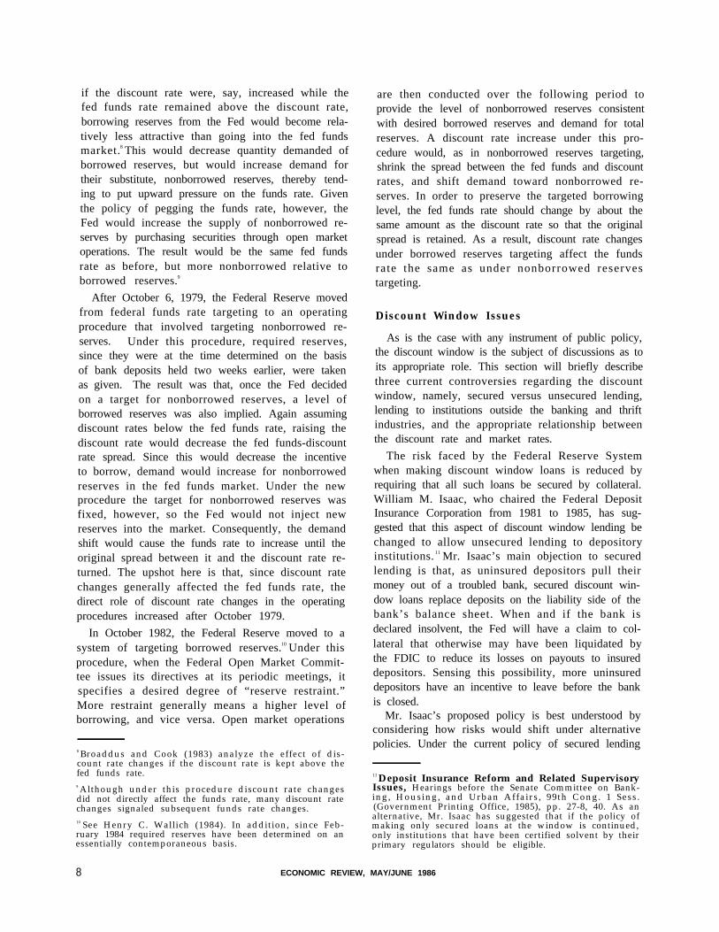
A striking feature is the amount of economicgrowth that is revealed. Chart 1 illustrates the move-ment of real GNP from 1929 to 1985. Despite theGreat Depression and other fluctuations, real GNPincreased fivefold during that interval-a 2.9 percentcompound annual rate of growth. Chart 1 also il-

4 Some arcane adjustments for households’ dealings withfinancial institutions are also included. Those adjust-ments also affect estimates of consumer spending for fi-nancial services.

Chart 1

REAL GNP

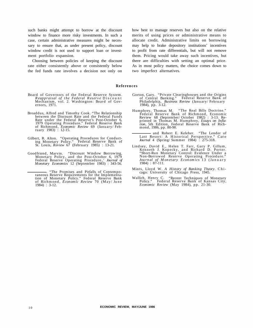
lustrates the massive decline of real GNP duringthe Great Depression, the equally massive expansionduring World War II, and the smaller fluctuationsof output in the postwar period. Chart 2 revealssimilar growth, but less fluctuation, in real consumerspending and disposable income.

The accounts also reveal some important changesin the structure of the economy. The expanded roleof government is illustrated by its spending for goodsand services, which has risen from less than 9 percentof GNP in 1929 to more than 20 percent in 1985.Foreign trade also plays a more important role inthe economy than it has in the past, with exportsrising from about 5 percent of GNP in the 1930s to11 percent in the 1980s.

Chart 2

CONSUMER SPENDING & INCOME


Cautions

Considering the amount of data consistently meas-ured over time and the complex interrelations re-vealed among disparate items, the national incomeand product accounts are a remarkable achievement.In part because the accounts do so much so well,users can be tempted to expect more of the accountsthan they can deliver. A few potential problems havealready been mentioned; in this section other po-tential pitfalls are discussed.

First, it should be emphasized that the national in-come and product accounts only measure production,spending and income. They were not designed tomeasure economic welfare-that is, how highly in-dividuals evaluate the economic rewards they receiveminus the cost of obtaining them. Despite the limit-ed focus of the accounts, it is still common for someobservers to see differences in national product be-tween nations as evidence of different standards ofliving. Such comparisons should be discounted formany reasons, a few of which follow:

(1) Some items included in GNP do not di-rectly raise individual welfare. For example, mili-tary spending is like intermediate product-it canprovide necessary protection that allows othereconomic activity to proceed, but is not valued forits own sake. Citizens of a nation that is able toobtain adequate defense for 1 percent of GNP canconsume and invest more, thus having a higherstandard of living, than citizens of a nation withthe same GNP who had to spend 10 percent ofGNP for defense.

(2) Some items are not included in GNP thatdo make people better off. For example, unpaidhousehold work may be highly productive but isnot included in the national income and productaccounts.

(3) There may be unmeasured external effectsthat result from productive activity. For example,the production of electric power may involve an un-measured damage of pollution from burning coal.Two countries could have the same GNP but dif-fer in the cleanliness of air and water.

(4) Other countries may use different datasources or even different concepts to produce in-come and product estimates. Socialist countries,for example, will lack many market prices usedin the U. S. accounts, Also different governmentsmay not have access to similar quantities or quali-ties of data.

A second caution is that it is possible that the defi-nition of an item in the accounts may not be thebest definition for a particular study.

For example, many economists have studied therelationship between consumer saving at one timeand consumer spending during later time periods.The definition of saving in the accounts is probablynot appropriate for that question, however, sincecapital gains and losses are excluded from per-sonal income and saving (because they do notresult from current production). Their potentialimportance is illustrated by rising stock and bondmarkets in 1985, which added hundreds of billionsof dollars to consumer wealth but were not incomeor saving as defined in the income and productaccounts.

Third, the construction of the national accountsrequires choosing among alternatives that each hasdrawbacks. One example is converting nominal ex-penditures to real magnitudes. The decision to esti-mate constant dollar values has greatly enhanced theutility of the accounts. There are side effects, how-ever.

The BEA’s approach is to define one year as abase year and to compare conditions in other yearswith the base year. That is, “real” magnitudes inother years are hypothetical values, such as quanti-ties exchanged in 1960 valued at prices paid intransactions in 1982. Constructing those hypo-thetical values allows the tracking of changes involumes of particular items over time, but can alsodistort relationships in the accounts. For ex-ample, from 1958 to 1973 net exports in currentdollars were positive each year, averaging over $7billion. When measured in 1982 dollars, however,net exports were negative in 15 of the 16 years,averaging -$18 billion. The actuality of a tradesurplus was therefore converted into a “real”deficit by using 1982 as a base period.

Fourth, the data that the BEA receives from othergovernment agencies may not be accurate.

For example, to the extent that individuals orfirms file inaccurate tax returns in order to reducetheir tax liabilities, the tax collectors will give theBEA inaccurate data. Moreover, if someone hasgiven false information to one government agency,the likelihood of that person giving false reportsto other agencies is increased. Census surveys,therefore, could also be affected by tax-inducedmisreporting of income and expenditure. Although


the BEA does attempt to estimate tax-inducedmisreporting, there is no way to determine the ac-curacy of those estimates.

These cautions should not prevent one from usingthe accounts. Rather, the cautions should prompt theuser to think about the problem and the data beforesimply assuming that the data are appropriate. Thelimitations of the accounts are real, but should bekept in perspective. The accounts provide consis-tently estimated data for more than fifty years forhundreds of items. They provide an unsurpassedpicture of economic performance. As the longtimehead of the BEA George Jaszi put it, the income andproduct accounts “are eminently useful in macro-economic analysis if they are not regarded as a pre-cision instrument and . . . may be lethal if they are.”

Suggestions for Additional Reading

There is a large literature on the subject of na-tional income and product accounts. Rather thanattempting to survey the whole field, a few sourcesare mentioned which should be especially helpful toreaders who wish to pursue the subject.

The Survey of Current Business (SCB), pub-lished monthly by the Commerce Department, con-tains recent estimates of items in the income andproduct accounts and articles on selected topics re-lated to national income accounting. One of themost useful publications on the subject is the N a -tional Income supplement to SCB, 1954 edition, partsII-IV. It contains 132 large format pages of detaileddefinitions and discussion of the methodology for

estimating components of the accounts. More recentdiscussions are contained in “The National Incomeand Product Accounts of the United States: AnOverview,” SCB February 1981, and “An Introduc-tion to National Economic Accounting,” SCBMarch 1985.

For many readers, less technical summaries of theaccounts may be useful. Introductory economics text-books usually contain descriptions of the accounts ; aparticularly good presentation is contained in PaulSamuelson’s Economics. Also, The U.S. EconomyDemystified by Albert T. Sommers has a clear, user-oriented description and discussion of the accounts.

Building on the framework of the BEA’s accounts,Robert Eisner has constructed a set of statistics thatattempt to narrow the gap between national productaccounts and statistics that more directly attempt toestimate economic welfare. “The Total IncomesSystems of Accounts,” SCB January 1985, containsa discussion of his approach and detailed tables ofdata for selected years.

Finally, it may be of interest to study the history ofnational income accounts. A prime source is John W.Kendrick, “The Historical Development of NationalIncome Accounts,” History of Political Economy,Fall 1970. A more narrow focus on U. S. accounts isgiven by Carol S. Carson, “The History of theUnited States National Income and Product Ac-counts,” Review of Income and Wealth, June 1975.Further insight into the design of the U. S. accountscan be found in George Jaszi’s “An EconomicAccountant’s Audit,” American Economic Review,May 1986.


CUMULATIVE PROCESS MODELS FROMTHORNTON TO WICKSELL

Thomas M. Humphrey

The celebrated Wicksellian theory of the cumu-lative process is a landmark in the history of mone-tary thought. It gave economists a dynamic, three-market (money, credit, goods) macromodel capableof showing what happens when banks, commercial orcentral, hold interest rates too low or too high. Withit one could trace the sequence of events throughwhich money, interest rates, borrowing, spending,and prices interact and evolve during inflations ordeflations. The prototype of modern interest-peggingmodels of inflation, it influences thinking eventoday. It also confirms the adage, well known tohistorians of science, that no scientific discovery isnamed for its original discoverer [19, p. 147]. For,as documented below, it was not Knut Wicksell butrather two British economists writing long beforehim in the first third of the nineteenth century whofirst presented the theory.

The cumulative process analysis itself attributesmonetary and price level changes to discrepanciesbetween two interest rates. One, the market ormoney rate, is the rate that banks charge on loans.The other is the natural or equilibrium rate thatequates real saving with investment at full employ-ment and that also corresponds to the marginal pro-ductivity of capital. When the loan rate falls belowthe natural rate, investors demand more funds fromthe banking system than are deposited there by savers.Assuming banks accommodate these extra loan de-mands by issuing more notes and creating more de-mand deposits, a monetary expansion occurs. Thisexpansion, by underwriting the excess demand forgoods generated by the gap between investment andsaving, leads to a persistent and cumulative rise inprices for as long as the interest differential lasts.As stressed by Wicksell, the differential vanishesonce banks raise their loan rates to protect their goldreserves from depletion by cash drains into hand-to-hand circulation. Given the volume of real trans-actions paid in gold coin, these drains arise from the

price increases that necessitate additional coin forsuch payments. The differential also vanishes whena loan rate set above the natural rate produces fall-ing prices and a reversal of the cash drain. In thiscase, the resulting excess reserves induce banks tolower their rates toward equilibrium in an effort tostimulate borrowing. These adjustments, however,may occur too late to prevent substantial changes inprices.

From this analysis it follows that the monetary au-thority must strive to keep the money rate in linewith the natural rate if it wishes to maintain pricestability. To do this, it must raise or lower its ownlending rate as soon as prices show the slightesttendency to rise or fall and maintain that ratesteady when prices exhibit no tendency to move ineither direction. By following this rule, it eradicatesthe two-rate disparity that generates inflation or de-flation.

The foregoing model and its policy implicationsare well known. Not so well known, however, is thatthe model was already more than 70 years old whenWicksell presented it in his Interest and Prices in1898. Long before then, Henry Thornton (1802,1811) and Thomas Joplin (1823, 1828, 1832) hadalready constructed versions of the model and hademployed it in their policy analysis. The model’stwo-rate, saving-investment, loanable-funds frame-work was as much their invention as Wicksell’s.The same is true of their demonstration that inflationstems from usury ceilings and bankers’ attempts topeg loan rates at levels other than those that clearthe market for real capital investment. Eventhe model’s famous equilibrium conditions-two-rate equality, saving-investment equality, loan-savingequality, aggregate demand-supply equality, mone-tary and price stability-were recognized by them.All they lacked was an automatic stabilizing mecha-nism that brings the cumulative process to a halt bythe convergence of the loan rate on the natural rate.


And this was provided by Wicksell in the form ofthe feedback effect of price changes on the loan rate.In an attempt to correct some misconceptions aboutthe theory’s origins and to give these pioneers theirdue, the paragraphs below outline the model and itscomponents to show what the three contributors hadto say about each.

The Model and Its Components

To identify the specific contributions of Wickselland his predecessors, it is useful to have some ideaof the model they helped create. As presented here,that full-employment model consists of seven equa-tions linking the variables investment I, saving S(both planned or ex ante magnitudes), loan rate i,natural rate r, excess aggregate demand E, money-stock change dM/dt, and price-level change dP/dt.1

Of these, saving and investment are taken to be in-creasing and decreasing linear functions of the loanrate, the presumption being that higher rates en-courage thrift but discourage capital formation.

The first equation states that investment I exceedssaving S when the loan rate of interest i falls belowits natural equilibrium level r (the level that equili-brates saving and investment),

where a is a coefficient relating the investment-savinggap to the rate differential that creates it. Thesecond equation states that the excess of investmentover saving equals the extra money dM/dt createdto finance it,

That is, assuming banks create money by way ofloan, monetary expansion occurs when they lendmore to investors than they receive in deposit fromsavers, To see this, denote the (investment) de-mand for loans LD as LD = I(i), where I(i) is theschedule relating desired investment spending to theloan rate. Similarly, denote loan supply Ls as thesum of saving S(i)-all of which is assumed to bedeposited with banks-plus new money dM/dt cre-ated by banks in accommodating loan demands ; inshort, Ls = S(i) + dM/dt. Equating loan demandand supply (LD = Ls) yields equation (2) above.

1 For similar models, see Eagly [2] and Laidler [10,pp. 104-5, 117].

The model’s third equation says that an excess ofinvestment over saving at full employment generatesan equivalent excess demand E for goods,

(3 ) I - S = E ,

as aggregate real expenditure outruns real supply.The fourth equation says that this excess demandbids up prices, which rise by an amount dP/dt pro-portionate to the excess demand,

(4) dP/dt = kE.

Substituting equations (1) and (3) into (4), andequation (1) into (2), yields

(5) dP/dt = ka(r - i) and

(6) dM/dt = a(r - i ) ,

which together state that price inflation and themoney growth that underlies it both stem from thediscrepancy between the natural and loan rates ofinterest. This, of course, is the model’s most famousprediction.

Finally, the seventh equation closes the model bylinking loan rate changes di/dt to price changesdP/dt. It states that bankers adjust their rates up-ward in proportion to the price rises so as to protecttheir gold reserves from being exhausted by inflation-induced cash drains into hand-to-hand circulation.That is, assuming the public makes a certain pro-portion of its real payments in the form of coin,rising prices increase the quantity of coin requiredfor that purpose. To arrest the resulting drain ofcoin reserves into hand-to-hand circulation, bankersraise their loan rates by an amount di/dt pro-portionate to price changes dP/dt,

(7) di /dt = b dP/dt .

This equation ensures that the loan rate eventuallyconverges to its natural equilibrium level, as can beseen by substituting equation (5) into equation (7)and solving the resulting differential equation for thetime-path of the loan rate.2 At this point, saving

2 Solving the differential equation di/dt = bka(r-i) ob-tained by substituting equation (5) into equation (7)yields the expression for the time-path of the loan rate i,

i ( t ) = ( i0 - r ) e - b k a t + r

where t is time, e is the base of the natural logarithmsystem, i0 is the initial disequilibrium level of the loanrate, and r is the (constant) natural rate. This expres-sion states that the loan rate will converge on the naturalrate with the passage of time if the coefficients b, k, anda are each positive, as is assumed in the model in the text.


equals investment, excess demand vanishes, moneyand prices are stable, and bank lending equals saving-these results obtaining when one sets the two ratesequal to each other in the model. These of courseare the famous Wicksellian conditions of monetaryequilibrium. Given the model and its components,one can identify what Wicksell and his precursorscontributed to it.

Henry Thornton

The origins of the cumulative process model are tobe found in Chapter 10 of Henry Thornton’s classicAn Enquiry into the Nature and Effects of the PaperCredit of Great Britain (1802) and in the first ofhis two parliamentary speeches of 1811 on the Bul-lion Report. In those works he contributed fourideas that together constitute the central analyticalcore of the model. He also demonstrated the model’spower as a tool of policy analysis.3

First, he noted that the quantity of loans demandeddepends upon a comparison of the loan rate of in-terest with the expected rate of profit on the use ofthe borrowed funds. He says, “In order to ascertainhow far the desire of obtaining loans at the bank maybe expected at any time to be carried, we must en-quire into the subject of the quantum of profit likelyto be derived from borrowing there under the exist-ing circumstances. This is to be judged of by con-sidering two points: the amount, first of interest tobe paid on the sum borrowed; and, secondly, of themercantile or other gain to be obtained by the em-ployment of the borrowed capital. . . . We may,therefore, consider this question as turning principallyon a comparison of the rate of interest taken at thebank with the current rate of mercantile profit”[20, pp. 253-4]. He continues : “The borrowers, inconsequence of that artificial state of things which isproduced by the law against usury, obtain their loanstoo cheap. That which they obtain too cheap theydemand in too great quantity” [20, p. 255]. Thusa loan rate equal to the profit rate limits loan de-mands to noninflationary levels. But a loan ratebelow the profit rate induces additional-and infla-tionary-loan demands.

Second, he explained how the rate differential,through its effect on loan demands, translates intomoney and price level changes. As noted above, therate differential induces an expansion of loan de-mands. Assuming that bankers accommodate these

3 On Thornton, see Hayek [4, pp. 12-14; 20, pp. 49-50]and Schumpeter [18, pp. 720-4].

loan demands by increasing their note issue-an as-sumption that implies a willingness to let reserveto note and deposit ratios fall-the money stock ex-pands. The resulting money-induced rise in aggre-gate expenditure puts upward pressure on prices. Italso, because of an assumed sluggish adjustment ofwages and other costs to rising prices, stimulates out-put and employment. Given that the economy nor-mally operates close to its full-capacity ceiling, how-ever, the price effect predominates. It follows thatprice inflation as well as the money growth that un-derlies it stems from the differential between the loanand profit rates as indicated by the expressionsdP /d t = ka ( r - i ) and dM/d t = a ( r - i ) . Here i sthe first model to show that inflation occurs whenbank rates are pegged at inappropriate levels.

Third, he stressed that the rate differential, if main-tained indefinitely, produces cumulative (continuing)rather than one-time changes in money and prices.This is so, he said, because as long as the loan rateremains below the equilibrium rate, borrowing willcontinue to be profitable (“the temptation to borrowwill be the same as before”) even at successivelyhigher price levels. The result will be more borrow-ing, more lending, more monetary expansion, stillhigher prices and so on without limit in a cumulativeinflationary spiral. Under these conditions, “eventhe most liberal extension of bank loans” will fail tohave the slightest “tendency to produce a permanentdiminution of the applications to the bank for dis-count” [20, p. 256]. On the contrary, loan demandswill be insatiable while the rate differential lasts.

Fourth, from the foregoing considerations Thorn-ton derived his fundamental equilibrium theorem,namely that monetary and price level stability obtainwhen the loan rate equals the profit rate. Such two-rate equality, he said, would allow the banking sys-tem to “sufficiently limit its paper” to noninflationarylevels “by means of the price [i.e., rate] at which itlends” [20, p. 254]. For with the two rates equal,their differential would vanish and with it the in-ducement to borrow and lend that produces infla-tionary money growth. Money and prices would stoprising and stabilize at a constant level. Having de-scribed the two-rate equilibrium, however, he did notexplain what forces would drive banks to attain it.His model lacked the automatic equilibrating mecha-nism through which inflation induces banks to raisetheir loan rates to equilibrium in order to protecttheir reserves from cash drains into hand-to-handcirculation.


Thornton’s Policy Conclusions

Thornton’s fifth contribution was his demonstra-tion of the model’s usefulness as a tool of policyanalysis. He used his model to determine the causeof the paper pound’s depreciation on the foreign ex-changes during the Napoleonic wars when Britainhad suspended the convertibility of her currency intogold at a fixed price upon demand. He attributedthe depreciation to note overissue caused by the Bankof England’s discount rate being too low. Usury ceil-ings, he noted, constrained the Bank’s rate to a 5percent maximum at a time when, owing to the boomconditions of the war, the expected rate of profit waswell in excess of 5 percent. The result of this dif-ferential was a loss of Bank control over the volumeof its loans and its note issue, both of which hadexpanded to produce inflation. To give the Bank afirm grip on the money supply, he urged removingthe usury ceiling and requiring the Bank to set itsdiscount rate equal to the profit rate. As a second-best alternative, he endorsed the Bank’s policy ofrationing loans. Apart from such direct credit ration-ing, however, he saw no end to inflation as long asthe differential persisted. In this connection, henoted that no amount of monetary expansion couldlower the profit rate to the level of the discount rate.The profit rate, he said, is a real variable determinedby the demand for and supply of real capital. Assuch, it is invariant with respect to changes in nom-inal variables like the money stock. Somewhat in-consistently, he admitted that money growth couldstimulate capital formation through forced saving-the inflation-induced redistribution of purchasingpower from fixed-income receivers to capitalist in-vestors. But he thought such effects to be quantita-tively unimportant. For that reason, he made nomention of the resulting capital accumulation’s im-pact on the profit rate.

He also employed his model to refute the real billsdoctrine according to which inflationary overissue isimpossible as long as banks lend only on sound com-mercial paper arising out of real transactions ingoods and services. He contended that the real billstest provided no check to overissue when the loan rateis below the profit rate. For the resulting price riseemanating from the differential would, by raising thenominal value of real transactions, in&ease the nomi-nal volume of eligible bills coming forward for dis-count. Since these bills would pass the real billstest (i.e., they are backed by an equivalent value ofgoods) they would be discounted and the moneystock would expand. This monetary expansion

would validate a further rise in prices thereby re-sulting in more bills being presented for discountleading to further monetary expansion and stillhigher prices and so on ad infinitum in a never-ending inflationary spiral. These examples show thatfor Thornton the cumulative process model was nota theoretical toy but a key component of his policyanalysis.

Thornton’s Contemporaries

Thornton’s two-rate analysis was accepted by atleast four of his contemporaries. Thus J. R. Mc-Culloch, in his refutation of the real bills doctrine,argued that loan demands depend primarily on “therate of interest for which those sums can be obtained,compared with the ordinary rate of profit that maybe made by their employment” [13, p. 235]. Simi-larly, Lord King warned that such loan demands“may be carried to any assignable extent” if the ratedifferential persists [9, p. 22]. John Foster put thepoint even more forcefully. He said that if the di-rectors of the Bank of England were to expand thenote issue in an effort to accommodate all loan de-mands arising at the disequilibrium rate, they “mightat length reduce the value of their notes to that of thepaper on which they are engraved” [3, p. 113]. Butperhaps the clearest and most succinct statementcame from David Ricardo who wrote that “The ap-plications to the Bank for money, then, depend on thecomparison between the rate of profits that may bemade by the employment of it, and the rate at whichthey are willing to lend it. If they charge less thanthe market [i.e., natural] rate of interest, there is noamount of money which they might not lend,-if theycharge more than that rate, none but spendthrifts andprodigals would be found to borrow of them. Weaccordingly find, that when the market rate of in-terest exceeds the rate of 5 per cent at which theBank uniformly lend, the discount office is besiegedwith applicants for money; and, on the contrary,when the market rate is even temporarily under 5 percent, the clerks of that office have no employment”[17, p. 364].

Missing from the analysis of Thornton and hiscontemporaries was any mention of the model’s realsaving and investment schedules. These componentswere largely overlooked before the appearance ofThomas Joplin’s Outlines of a System of PoliticalEconomy (1823), Views on the Currency (1828),and An Analysis and History of the Currency Ques-tion (1832).


Thomas Joplin

Joplin incorporated saving and investment sched-ules into Thornton’s model and defined the naturalrate as the rate that equilibrates the two.4 He thenargued that an increase in the demand for capital, byraising the natural rate above the loan rate, will opena saving-investment gap and a corresponding excessdemand for goods that bids up prices progressivelyas long as the rate differential lasts. He likewisenoted that money growth would accompany and vali-date the price increases as bankers (who have noway of knowing what the natural rate is and socharge their customary rate) honor all credit de-mands at the going loan rate. These considerationsled him to conclude with Thornton that monetaryand price level changes stem from disparities betweenthe two rates. He also concluded that monetaryequilibrium and its attendant balance conditions-saving-investment equality, loan-saving equality, ag-gregate demand-supply equality, monetary and pricelevel stability-obtain only when the two rates areequal.

Joplin’s observations are so Wicksellian thatthey must be read to be believed. On the relationI-S=dM/dt between the investment-saving gap andthe monetary change that finances it, he wrote,“When the supply of capital exceeds the demand,it has the effect of compressing it [the circula-tion]; when the demand is greater than the supply,it has the effect of expanding it again” [8, p. 101].On the express ion dM/d t=a( r - i ) connec t ingmoney-stock changes with the natural rate-loan ratedisparity, he remarked that since bankers “never canknow what the true [natural] rate of interest is”they “charge a fixed [loan] rate,” with the conse-quence that the currency “expands and contracts, in-stead of the interest of money rising and falling”[8, pp. 109, 111].

Likewise, on the mechanism through which devia-tions of the loan rate from the natural rate produceinflation, he observed, “Money comes into the market. . . from the banks . . . in consequence not of a de-mand for currency, but of a demand for capital, de-termined by the interest which the banks charge pro-portioned to the market [i.e., natural] rate. And inall cases the influx of money into the market . . . isnot the effect, but the cause of high prices” [6,

4 On Joplin, see Corry [1, pp. 54-6, 60-1, 110], Hayek[4, pp. 15-7], Link [12, pp. 73-102], Schumpeter [18,p. 723], Viner [22, pp. 190-2], and Warburton [23, pp. 125,290].

pp. 258-9]. Here is an explicit recognition of (1)the two-rate disparity, (2) the investment demandfor loans, (3) a loan-determined money stock, and(4) the money-price relationship-all key ingredientsof Wicksell’s analysis. Finally, on pegging the loanrate above the natural rate so that saving exceeds in-vestment and loans, money, and prices all fall, hesaid, “If it [fall of prices] proceeded from the interestcharged by the banks, being too high, the economy[i.e., saving] of the country, instead of reducing theinterest . . . would find vent in discharging the debtsdue to the banks, at the high rate of interest they im-posed; and the value of money and profits of tradewould thus be kept up to that level which renderedthe general economy [saving] greater than the gen-eral expenditure [investment]” [6, pp. 209-10].Here is perhaps the first application of the cumula-tive process model to the deflationary case in whicha loan rate above the natural rate spells an excess ofsaving over investment, a deficiency of aggregate de-mand, a contraction of borrowing and the moneystock, and a consequent fall of prices. In otherwords, Joplin recognized that interest-rate peggingcan lead to deflation as well as inflation.

Like Thornton, he saw forced saving as one effectof the price inflation produced by banks’ willingnessto lend more than the savings voluntarily depositedwith them. “If the issues of the bank are not in-creased by any loan it makes at interest, an equalamount of money must have been previously savedout of income, and paid into the bank, in which case,the party borrows the income previously saved ; butif not, and the issues of the bank are increased bythe loan, prices rise, and the party who has borrowedthe money obtains value for it by depriving the hold-ers of the money in previous circulation, of a pro-portionate power of purchasing commodities. Aneconomy is thus created, though a forced economy,but it answers all the purpose of a volutary one”[7, p. 146]. He opposed forced saving on thegrounds that it involved a fraud and an injustice onthe preexisting money holders.

From his analysis he concluded that interest-ratepegging is an important cause of price-level fluctua-tions. “One effect, no doubt, would be produced bythe bank regulating its issues by the demand for[loans] at a particular rate of interest, namely, thatthe rate of interest would be kept steady. Instead ofthe savings of income rising above four per cent [fol-lowing, say, an upward shift in the loan demandschedule], the enlargement of issues would create anadditional quantity sufficient to supply, at four per


cent, the increased demand. On the other hand,when the savings of income were not in such request,and the demand at four per cent fell off, the notes ofthe bank would be withdrawn, and the supply of suchsavings, to a corresponding extent, would be cancel-led, by which the rate of interest would be kept up[above its natural level]. The alteration in the[loan] demand for capital would not affect its value.The supply of it by means of the enlargement andcontraction of the currency, would be created andcancelled as it was required. Prices would fluctuateinstead of the interest of money” [7, pp. 152-3].

He contended that these price fluctuations occurbecause banks possess the power of creating and de-stroying paper money at will by varying their reserveratios. Take away this power, he said, and bankswould become pure intermediaries, lending only thesavings entrusted to them. In this case, saving wouldequal investment, loan rates would equal the naturalrate, excess demand would be zero, and price sta-bility would prevail. To make these equilibrium con-ditions a reality he proposed a policy of 100 percentrequired gold reserves behind note issues.

To summarize, Joplin gave the model its mostcomplete formulation up to Knut Wicksell. His in-clusion of saving and investment schedules allowedhim to show how gaps between the two produced bydeviations from the natural rate translate into money-stock changes and excess demand that bids up prices.In short, he recognized all the model’s componentsexcept the price-induced interest-adjustment mecha-nism that ensures the stability of monetary equi-librium.

Knut Wicksell

When Wicksell presented his cumulative processmodel in 1898, he thought he was the first to do so.5

At that time he was totally unaware of the earlierwork of Thornton and Joplin. Not until 1916 did hediscover from his colleague David Davidson thatThornton had foreshadowed him by almost 100 years.But he apparently never learned about Joplin, whosesaving-investment version of the model was virtuallyidentical to his.

One finds in his model all the elements developedby Thornton and Joplin. The two-rate disparity isthere, as are the saving-investment gap, the excessdemand for goods that bids up prices cumulatively,

5 On Wicksell, see Jonung [5], Laidler [10], Leijonhu-fvud [11, pp. 151-61], Patinkin [15, pp. 587-97; 16] andUhr [21, pp. 198-254].

and the accompanying money growth resulting frombanks’ willingness to accommodate all credit demandsat the going loan rate. His conclusion-that mone-tary and price-level changes stem from the two-ratedisparity-is the same as theirs. So too is his list ofmonetary equilibrium conditions, including two-rateequality, saving-investment equality, loan-savingequality, aggregate demand-supply equality, andmonetary and price-level stability. True, he differedfrom Joplin on how these conditions should beachieved. He preferred a policy of promptly movingthe discount rate in the same direction as prices arechanging, stopping only when price movementscease. By contrast, Joplin preferred a policy of 100percent required gold reserves. But both believedthat there existed a workable policy rule to keepmoney rates in line with the natural rate. Like hispredecessors, he even used his model as a tool to ex-plain British price movements in the nineteenth cen-tury, although he focused on secular rather thancyclical changes.

He differed from Thornton and Joplin chiefly inhis inclusion of the stabilizing feedback effect ofprice-level changes on the loan rate. By adding thiselement to the model he was able to show that thecumulative process is self-limiting provided banksmaintain some desired level of gold reserves and pro-vided the public transacts a certain proportion of itsreal payments in gold coin. Since inflation increasesand deflation decreases the need for coin in circula-tion to effectuate these given real payments, banks,he argued, will find their reserves being depleted inthe former case and augmented in the latter. Toarrest these price-induced reserve drains or accumu-lations they will adjust their rates upward or down-ward. In this way those price changes bring theirown cessation as the loan rate converges on the na-tural rate.

He also demonstrated that the cumulative processis not self correcting in hypothetical “cashless” orpure credit economies using no metallic money, allpayments being made by bookkeeping entries, Sincespecie drains are not a threat in such economies,banks need hold no reserves and are free to maintainindefinitely any money rate they choose. As a result,there exists no reserve constraint in the cashless so-ciety to limit the cumulative process. Thus anyspontaneous disturbance that upsets the initial equal-ity between the two rates will set in motion an in-flation or deflation that can continue indefinitely.He further argued that the same may be true evenin pure cash societies if technological innovations,

FEDERAL RESERVE RANK OF RICHMOND 23

wars, and other real shocks cause the natural rateto change before the loan rate can ever catch up withit. In this case, the loan rate’s lag behind the movingnatural rate spells incomplete adjustment, persistentdisequilibrium, and ceaseless price changes.

This last insight, which combined the notions ofan active or leading natural rate and a passive ortrailing loan rate, enabled him to resolve what Keyneswas later to call the Gibson paradox. This paradox,which neither Thornton nor Joplin addressed, holdsthat prices and interest rates historically move to-gether in the’ same direction when, according tostandard monetary theory, they should move inverse-ly as excess issues of money temporarily depress in-terest rates while raising prices. In resolving theparadox, Wicksell agreed that prices and loan rateswould move inversely if those rates fell below a givennatural rate. For example, if loan rates fell to 4 per-cent when the natural rate was 5 percent, priceswould rise. On the other hand, prices and loan rateswould tend to move together if the natural rate itselfmoves and the loan rate lags behind (i.e., adjustsincompletely to the changing natural rate). In thiscase, loan rates, though rising or falling, would stillbe too low or too high relative to the natural rate toprevent a cumulative rise or fall in prices. Indeed,this was precisely Wicksell’s explanation of long-term price changes in nineteenth century Britain.These changes he saw as emanating from movementsof the active natural rate about the lagging loan rate.Except for these applications, Wicksell’s use of themodel was the same as Thornton’s and Joplin’s.

Concluding Comments

That Wicksell at best only rediscovered or rein-vented the model now universally associated with hisname is hardly surprising. It merely confirms thevalidity of Stigler’s Law of Eponymy according towhich no scientific discovery is named for its originaldiscoverer. Still this finding, though completely un-exceptional, is nevertheless at odds with some recentinterpretations of the model’s history. Certainly itis not true, as suggested in Axel Leijonhufvud’s re-cent essay on the “Wicksell Connection,” that themodel derives solely from Wicksell. Nor is it true, asLeijonhufvud contends, that Wicksell originated thesaving-investment approach to macroeconomics [11,pp. 132-3]. For, as documented above, the cumula-tive process model together with its implied con-ditions of monetary equilibrium originated not withWicksell but rather with Thornton and Joplin. Ofthese two pioneers, Joplin deserves at least some

credit for initiating the saving-investment approachsince it was he who first introduced saving and in-vestment schedules into the model.

These findings also cast doubt on Robert Nobay’sand Harry Johnson’s recent attempt to distinguishbetween classical and Wicksellian phases in the evo-lution of monetary thought [14, pp. 471-3]. Theclassicals, according to this distinction, concentratedon establishing the proposition of the long-run neu-trality of money. Wicksellians, by contrast, focusedon the dynamic implications of monetary responsesand disturbances as well as on the conditions ofmonetary equilibrium. What is overlooked is thatat least two classical monetary theorists, namelyThornton and Joplin, were Wicksellians as far astheir monetary analysis was concerned. True, theyaccepted the neutrality proposition. But their mainconcern was investigating the dynamics of money’sresponse to deviations of the loan rate from the nat-ural rate. They also sought to eliminate those de-viations so that prices could be stabilized. To thatend they spelled out the conditions of monetaryequilibrium and prescribed policies to achieve them.In these ways they strongly resembled Wicksell.

References

1. Carry, B. A. Money, Saving and Investment in Eng-l ish Economics: 1800-1850. New York: St. Mar-tin’s Press, 1962.

2 . E a g l y , R . “A Wicksell ian Monetary Model: AnExpos i tory Note .” Scottish Journal of Polit icalEconomy (June 1966), pp.. 251-54. Reprinted inhis The Structure of Classical Economic Theory.N e w Y o r k : O x f o r d U n i v e r s i t y P r e s s , 1 9 7 4 ,pp. 86-9.

3 . Foster J . L. An Essay on The Pr inc ip l e s o f Com-mercial Exchanges. London: J . Hatchard, 1804.

4. Hayek, F. A. v. Pr i c e s and Produc t i on . 2 n d E d i -tion. London : Routledge, 1935.

5. Jonung, L. “Knut Wicksell and Gustav Cassel onS e c u l a r M o v e m e n t s i n p r i c e s . ” J o u r n a l o fMoney, Credit and Banking 11 (May 1979),165-81

6. Joplin, T. Outlines of a System of Polit ical Econ-o m y (1823). New York: Kelley, 1970.

7 Views on the Currency. London: J . Ridg-way, 1828.

8 . An Analysis and History of the CurrencyQuestion. London: J . Ridgway, 1832.

9 . K i n g , P . T h o u g h t s o n t h e E f f e c t s o f t h e B a n kRestriction. London: Cadell and Davis, 1803.

10. Laidler, D. “On Wicksell’s Theory of Price LevelDynamics.” The Manches t e r Schoo l 4 0 ( J u n e1972), 125-44. Reprinted in his Essays on Moneyand Inflation. Chicago : Univers i ty o f ChicagoPress, 1972, pp. 101-19.


11. Leijonhufvud, A. “The Wicksell Connection: Var-iations on a Theme.” Chapter 7 of his In f o rma-t i o n a n d C o o r d i n a t i o n : E s s a y s i n M a c r o e c o -nomic Theory . New York : Oxford Univers i tyPress, 1981.

12 . L ink , R . G . E n g l i s h T h e o r i e s o f E c o n o m i c F l u c -tuations 1815-1848. New York: Columbia Uni-versity Press, 1959.

13. McCulloch, J . R. Notes to the Wealth of Nations.Vol. 4. (1828).

14. Nobay, A. R., and H. G. Johnson. “Monetarism:A H i s t o r i c - T h e o r e t i c P e r s p e c t i v e . ” Journal ofEconomic Literature 15 (June 1977) , 470-85.

15. Patinkin, D. Money, Interest, and Prices. 2nd Edi-tion. New York: Harper and Row, 1965.

16. .“Wicksell’s Cumulative Process in Theoryand Practice.” B a n c a N a z i o n a l e d e l L a v o r oQ u a r t e r l y R e v i e w (June 1968), pp. 120-31. Re-printed in his Stud i e s in Mone tary Economics .New York: Harper and Row, 1972, pp. 83-91.

1 7 . R i c a r d o , D . The Pr inc ip l e s o f Po l i t i c a l Economya n d T a x a t i o n ( 1 8 1 7 ) . E d i t e d b y P . S r a f f a .London: Cambridge University Press, 1951.

18 . Schumpter , J . A . His to ry o f Economic Ana lys i s .London: George Allen and Unwin, 1954.

19 . S t ig ler , S . “S t ig ler ’ s Law of Eponymy.” T r a n s -ac t i ons o f t h e New York Academy o f Sc i ence s .Series II. Vol. 39 (April 24, 1980), 147-58.

20. Thornton, H. An Enquiry into the Nature and Ef-f e c t s o f t h e P a p e r C r e d i t o f G r e a t B r i t a i n(1802). Together with his evidence given before

the Committees of Secrecy of the two Houses ofParliament in the Bank of England, March andApril , 1797, some manuscript notes, and hisspeeches on the Bullion Report. May 1811. Edit-ed with an introduction by F. A. v. Hayek. NewYork : Rinehart and Co., Inc., 1939.

2 1 . U h r , C . E c o n o m i c D o c t r i n e s o f K n u t W i c k s e l l .Berkeley and Los Angeles: University of Cali-fornia Press, 1962.

22 . V iner , J . Stud i e s in th e Theory o f In t e rna t i ona lT r a d e . N e w Y o r k : H a r p e r , 1 9 3 7 . R e p r i n t e dNew York: Kelley, 1965.

23 . Warbur ton , C. Depre s s i on , In f l a t i on , and Mone -tary Policy : Selected Papers 1945-1953. B a l t i -more: Johns Hopkins Press, 1967.

24 . Wickse l l , K . In t e r e s t and Pr i c e s ( 1 8 9 8 ) . T r a n s -lated by R. F. Kahn. London: Macmillan, 1936.Reprinted New York: Kelley, 1965.


THE INDUSTRIAL MIX OF EMPLOYMENTIN THE FIFTH DISTRICT, 1950-1985

Christine Chmura*

The industrial distribution of employment in theUnited States has undergone significant changes overthe years. Once predominantly agricultural, thenation’s workforce first shifted from farming tomining and manufacturing, and then from producinggoods to producing services. The concentration ofemployment also has changed substantially withinmajor industrial classifications, such as from smoke-stack to high-tech manufacturing.

Regions within the United States generally displaythe same major industrial shifts in employment thathave occurred in the nation as a whole. But regionaleconomies do exhibit significant differences in em-ployment growth by industry and industry subgroups.A regional analysis of the industrial distribution ofemployment can therefore provide important insightsinto the development and current character of anarea’s economy. Such information may be of use tostate and local officials and to other citizens in theirefforts to attract industry and promote growth. It isalso of interest to citizens wishing to know why, how,and how much the employment mix in a region haschanged.

This article describes and analyzes the principalchanges in nonagricultural employment in the FifthFederal Reserve District during the past 35 years,with emphasis on more recent years. The mainfinding is that the employment trends in the FifthDistrict are similar to those of the nation, except thatthe percent of manufacturing employment has notdeclined as rapidly in the District as in the nation.The first section reviews developments in the UnitedStates as well as in the District and points out wheredifferences are significant. The second section ana-lyzes changes in the industrial employment mix. Thethird section focuses on employment changes inindustry subgroups within the manufacturing andservice sectors, again using national trends as a basis

* The author thanks Dan M. Bechter for his invaluablecomments.

for evaluating Fifth District developments. Thefourth and final section summarizes the findings anddiscusses some implications for the District.

I.

POSTWAR INDUSTRIAL EMPLOYMENT GROWTH

Since the end of World War II, total nonagricul-tural employment in the United States has increasedgreatly. Over that same period, dramatic shifts haveoccurred in the percentages of workers employed inspecific sectors or industries and in the regionalconcentration of employment by industry. While theFifth District’s postwar changes in employmentbroadly reflect those of the nation as a whole, thereare important differences.

The analysis focuses on changes from 1946 to thepresent.1 However, since trends are the topic ofinterest here, the years used for comparative purposesare chosen to minimize the effects of the businesscycle. Thus, most of the comparisons are based onemployment data for 1950, 1972, 1978, and 1985--all years of economic expansion that occur withinthree years after a business cycle trough.

Total Employment

The pronounced increase in nonagricultural em-ployment in the United States during the past 35years is shown in Figure 1. The doubling in jobsover this period translates to an average annualgrowth rate of 2.2 percent.

1 This analysis is based primarily on annual data fromthe U. S. Department of Labor. The data, known as the“payroll series,” provide detail on employment by indus-try and state. The labor force data are obtained from“establishment surveys.” That is, a firm operating inmore than one location must submit a report for eachestablishment. In addition, firms engaged in distinctlydifferent lines of activity are required to submit separatereports, if possible. For definitions of terms, area samplesused, historical comparability of the data, comparabilitywith other series, etc., see Department of Labor, Bureauof Labor Statistics, “Employment, Hours, and Earnings.”


Figure 1

U.S. NONAGRICULTURAL EMPLOYMENT

NOTE: District employment growth reflects the growthpattern in the United States.

Employment in the Fifth District also more thandoubled between 1950 and 1985. Jobs in the FifthDistrict grew at an average annual rate of 2.6 percent,with Virginia posting the strongest gain, followed inorder by North Carolina, South Carolina, Maryland,the District of Columbia, and West Virginia. (SeeTable I.) To be sure, over the more recent periodfrom 1972 to 1985 employment growth slowed inboth the nation and the Fifth District. But the Dis-trict rate remained above that of the nation, althoughnot by as great a margin as was recorded from 1950to 1972.

Table I

GROWTH IN EMPLOYMENT

Average annual rates

1950-72 1972-85* 1950-85*

United States 2.25 2.19 2.22

Fifth District 2.67 2.36 2.55

District of Columbia 0.64 0.73 0.67

Maryland 3.14 2.23 2.80

North Carolina 3 .34 2.53 3.04

South Carolina 3 .19 2.69 3.00

Virginia 3.33 3.05 3.23

West Virginia 0.14 0.76 0.37

* 1985 is a preliminary figure.

Growth differences among geographical regionsoccur for various reasons. Since World War II, theFifth District labor supply has increased faster thanthat of the nation because of a higher District birthrate in the 1950s and a migratory movement towardthe South in the 1960s and 1970s.2 Other factorscontributing to growth differences among geographi-cal areas will be considered later.

From Goods to Services

A major trend in the employment mix over thelast century has been a shift from goods-producingto service-producing industries.3 As shown in Figure2, employment in service-producing industries hasgrown significantly relative to employment in goods-producing industries in the United States. The sametrend has occurred in the District. The change inemployment reflects different rates of growth in pro-ductivity and demand which will be explained furtherin Section II.

2 For more explana t ion of the labor force composi t ion ,

see Lynn E. Brown, “Regional Unemployment Rates-Why Are They So Dif fe ren t?” New England EconomicReview, July/August 1978, pp. 9-11.3

The min ing , cons t ruc t ion , and manufac tur ing sec torsare of ten re fer red to as goods-producing because the i rproduc ts a re tangib le whi le the remain ing sec tors a recollectively termed service-producing.

Figure 2

EMPLOYMENT DISTRIBUTION OF GOODSAND SERVICES IN THE UNITED STATES

--- Goods-producing --- Service-producing

NOTE: The change in employment distribution of goodsand services in the District reflects that of theUnited States.


The United States and the District have beenservice economies in terms of employment since theearly 1900s when over 50 percent of the work forcebecame employed in service-producing industries.The trend toward services, however, has becomemore rapid since the 1950s. In fact, the U. S.service-producing sectors have as a group grown atan annual average rate of 2.9 percent between 1950and 1985, while the goods-producing sectors havegrown 0.9 percent per year. Within these two classi-fications, employment growth rates by individualsector vary considerably.

Sector by Sector

Figure 3 displays changes in the relative distribu-tion of employment in the United States and theFifth District by major industrial sector. (See Box.)Clearly evident is the great increase in the relativenumber of service sector employees.4 The servicesector has become the second largest employer in the

4 The service sector is defined more narrowly here thanin the previous section.

Figure 3

EMPLOYMENT SHARE BY MAJOR SECTOR

United States Fifth District1950 1950

nation and the District, growing between 1950 and1985 at an annual average rate of 4.1 and 4.5 percent,respectively.

In contrast, the relative share of the manufacuringsector has declined considerably. In 1950, U. S.manufacturing jobs comprised 33.7 percent of non-agricultural employment, but they declined to about19.8 percent in 1985. By comparison, the Districthad 31.5 percent of its employees in the manufac-turing sector in 1950 compared with only 20.4 percentin 1985. Despite the gradual decline in the manu-facturing sector share of total employment, there hasbeen an increase in the number of workers employed.Between 1950 and 1985, U. S. manufacturing em-ployment rose 27 percent while the Fifth Districtgain was nearly 57 percent.

A comparison of industry sector growth in theFifth District with that of the United States between1950 and 1972 reveals that the District gained em-ployment more rapidly than the United States in allindustries except mining and government. Both thenation and the Fifth District experienced trends inindustry employment over the last 13 years thatdiffered from their counterparts between 1950 and1972. As shown in Table II, the growth rate ofnonagricultural employment, national as well as Dis-trict, slowed between 1972 and 1985. Among thevarious sectors, employment in mining, transporta-tion and public utilities, wholesale and retail trade,and service grew faster in the last 13 years whileemployment in construction, manufacturing, andgovernment, grew considerably more slowly. Whenthe District’s industry sectors are examined relativeto the nation’s from 1972 through 1985, slowergrowth rates are found in the District’s mining andfinance, insurance, and real estate sectors.

II.

ANALYSIS OF CHANGES ININDUSTRIAL EMPLOYMENT MIX

The growth of employment in various sectors andregions differs dramatically. This section offers someexplanations for the different rates of employmentgrowth in the nation’s manufacturing and servicesectors and for the interregional disparities in theserates of growth.

Explanations of Manufacturing andService Sector Shifts

The industrial composition of U. S. jobs dependsprimarily on two factors : the type and mix of goods


Industrial Classifications

The Standard Industrial Classification (SIC) system defines sectors on the basis of suchfactors as end-product similarity, types of resources used, and types of customers. The eight majorSIC manual sectors are:

Mining - Businesses extracting minerals occurring naturally such as coal, ores, crude petroleum,and natural gas. Also included are operations necessary to make minerals marketable.

Construction - Builders and other fabricators producing new work, additions, alterations, andrepairs including special trade contractors, such as plumbing, painting, and electrical work.

Manufacturing - Firms performing mechanical or chemical transformations of materials or sub-stances into new products.

Transportation and Public Utilities - Establishments providing passenger and freight transpor-tation, communication services, electricity, gas, steam, water or sanitary services, and theU. S. Postal Service.

Wholesale and Retail - Places of business primarily engaged in selling merchandise for personal,household, industrial, commercial, institutional, farm, or professional business consumption,as well as firms engaged in the sale of goods to other wholesalers.

Finance, Insurance, and Real Estate - Establishments providing specialized activities in eitherthe finance, insurance, or real estate field.

Service - Establishments providing a wide variety of services for individuals, business and gov-ernment establishments, and other organizations.

Government - Organizations performing the legislative, judicial, administrative, and regulatoryactivities of federal, state, local, and international government.

LTable II

EMPLOYMENT GROWTH BY SECTOR

Average annual rates

United States Fifth District

1950 -72 1972 -85* 1950 -72 1972 -85*

Total Nonagriculture 2.25 2.19 2.67 2.36

Mining -1.63 3.07 -3.06 -0.56

Construction 2.29 1.45 3.30 1.53

Manufacturing 1.04 0.07 1.94 0.20

Transp. and Public Utilities 0.54 1.11 0.92 1.49

Finance, Ins., and Real Estate 3.36 3.29 4.17 3.06

Wholesale and Retail Trade 2.44 2.89 2.78 3.34

Service 3.84 4.58 4.24 5.04

Government 3.68 1.61 3.40 2.08

* 1985 is a preliminary figure.


and services desired by consumers, businesses, gov-ernments, and foreigners, and the differentials inlabor productivity by industry. By explaining thechange in the mix demanded and the changes inlabor productivity one can indirectly account for thecauses of the change in the industrial mix of em-ployment.

One reason for the shift from goods to servicesproduction is that people tend to demand more servicegoods relative to manufactured goods as incomerises. 5 There has been an increase in the proportionof the service sector contribution to the gross na-tional product (GNP) between 1950 and 1984. Thereal service sector GNP increased from 11.1 percentof total GNP in 1950 to 14.6 percent in 1984.6

The relative decline in manufacturing employmentalso reflects the much faster increase in output perworker in the manufacturing sector than in the ser-vice sector.7 Labor productivity indices show thatproductivity growth in the manufacturing sector hasexceeded the average rate of productivity growth inthe United States since 1960. In other words, theamount of labor required per unit of output fell morerapidly in the manufacturing sector than in othersectors. Consequently, the relatively smaller amountof labor required to produce a unit of output con-tributes to a relative decline in manufacturing em-ployment.

In support of the productivity argument, VictorFuchs many years ago argued that the relativelyhigher cost of manufacturing labor to service laborcaused a greater substitution of capital for labor inthe manufacturing sector.8 In this view, industriesreact to the cost differential by substituting the lowerpriced input for the higher priced input, where pos-sible. If manufacturers find it more profitable tosubstitute capital for labor, then the manufacturingshare of employment will decline while employmentin other sectors, such as services, will increase. Infact, the average hourly earnings for U. S. manu-facturing production workers was $9.18 in 1984

while service sector nonsupervisory workers earnedonly $7.64 per hour. The high percent of unioniza-tion in the manufacturing sector has contributed toits relatively high wages. Within the manufacturingsector, union wages increased 11 percent faster thannonunion wages between 1970 and 1984.9 Becauseof the relatively high cost of labor in manufacturing, agreater incentive to substitute capital for laborexisted ; hence a shift of the employment shares to theservice sector may have resulted.

Explanations of Shifts inRegional Employment

Two determinants influence shifts in the industrymix of a region’s labor force. First, there is the“industry factor,” defined as the base period industrymix of employment. The historical industry mixaffects future changes in employment because someregions possess a larger proportion of the nation’srapidly growing industries. Second, a region’s em-ployment changes are explained by the “regionalfactor,” defined as the competitive advantage oneparticular region has over other regions due, forexample, to low-cost inputs for specific industriesand access to important markets.

Competitive advantage, via its effect on plantprofitability at different sites, influences plant loca-tion and thereby regional employment. Numerousstudies, which are heavily oriented toward manu-facturing, have been conducted to determine therelationship between plant location and regionalcharacteristics. Among the variables reported tohave a positive impact on interregional and interstatemanufacturing location choice are lower wages, busi-ness taxes, personal income taxes, unionization, andhigher primary and secondary education spending.10

Thus employment in regions with attractive char-acteristics grows relatively faster than regions withunattractive characteristics.

In mining, more so than in other sectors, locationand, therefore, employment shifts are dependent upon

5 Everett E. Hagen, The Economics of Development,Fourth Edition. (Homewood, Illinois: Irwin, 1986), pp.

6 In the category of goods production manufacturing hasheld its own, increasing from 21.4 percent to 21.8 percentof GNP over the same period.7 See Victor R. Fuchs, The Growing Importance of theService Industries (New York: Columbia UniversityPress, 1965), pp. 13, 14, and Edward F. Denison, “TheShift to Services and the Rate of Productivity Changes,”Survey of Current Business 53 (October 1973), pp. 20-35.8 Fuchs, pp. 13, 14.

9 Colin Lawrence and Robert L. Lawrence, “Manufac-turing Wage Dispersion: An End Game Interpretation,”Brookings Papers on Economic Activity (1985:1), p. 48.10 For a study on wage differentials, see William E.Cullison, “Equalizing Regional Differences in Wages: AStudy of Wages and Migration in the South and OtherRegions,” Economic Review, Federal Reserve Bank ofRichmond 70 (May/June 1984), pp. 20-33. For an in-depth review of studies on business location decision, seeMichael Wasylenko, “Business Climate, Industry andEmployment Growth: A Review of the Evidence,” Met-ropolitan Studies Program, Syracuse University, Oc-casional Paper No. 98, October 1985.


the resource site. The District’s relative employmentdecline in mining, however, is primarily due to thedecrease in West Virginia mining at an average rateof 2.9 percent annually between 1950 and 1985.There has been a significant increase in coal produc-tion in the past decade, but the rapid rise in coalmining productivity has created a decline in employ-ment. In 1944, for example, over 393,000 bituminousand lignite miners produced an average 5½ tons perminer per day for a total production of 619 milliontons. In 1980, only 225,000 miners produced over16 tons per miner per day for a total output of 800million tons. The relative decline in Fifth Districtmining employment is also partly attributable to thelarge increase in surface mining in the western statesof the United States.

III.

FIFTH DISTRICT MANUFACTURING ANDSERVICE EMPLOYMENT SHIFTS

The most significant employment shifts within theDistrict and the nation have taken place in the manu-facturing and service sectors. The remainder of thispaper concentrates exclusively on these sectors.

The economic performance of the Fifth District isevaluated by comparing percentage changes in em-ployment of the United States with comparable fig-ures for the Fifth District. The period 1972 through1985 is chosen for the manufacturing comparisonbecause the 13-year period 1972-1985 is long enoughfor significant changes to have occurred. Further-more, both end-point years occur within three yearsafter a business cycle trough. For the service sectorcomparison, however, the years 1978 and 1984 arethe end points because comparable data are not avail-able prior to 1978 or later than 1984.11

The percent change in the District and each of itsstates is compared to that of the nation. The netemployment gain or loss of an area relative to theUnited States reflects faster or slower growth com-pared to the nation as a whole. Moreover, the changein composition of each state’s manufacturing or ser-vice sector indicates which industry subgroups hadthe greatest impact on the state’s total manufacturingor service growth.

11 Tables giving manufacturing employment (1972 and1985) and service employment (1978 and 1984) by statesin the Fifth District and for the District by SIC codes areavailable upon request from the author.

Fifth District vs. United States

Manufacturing Employment

At the national level, manufacturing employmentgains primarily occurred in high-tech jobs. On theother hand, employment losses were experienced bymanufacturers depending most on natural resources.The instruments and related products group-a high-tech manufacturing classification-grew faster thanany manufacturing group in the nation with a 40.2percent employment increase between 1972 and 1985.Large employment increases also occurred in electricand electronic equipment, machinery (except elec-trical), and printing and publishing. On the otherhand, primary metals experienced a 30.7 percent de-cline in employment followed by textile mill products(18.8 percent), and apparel (18.6 percent).

Figure 4 shows that manufacturing groups within

the Fifth District have undergone changes quite

different from those of the nation. Employment in

the Fifth District grew faster or declined more slowly

than in the nation in all but three of eighteen manu-

facturing industry groups. For example, Fifth Dis-trict apparel employment declined by 8.8 percent

between 1972 and 1985 while apparel employment inthe United States declined 18.6 percent. This differ-ential indicates that employment in the nationalapparel industry though declining overall is tendingto be more heavily located in the Fifth District.

Figure 4

MANUFACTURING EMPLOYMENT CHANGES

1972 - 1985


Explanations of Interstate Changes inManufacturing Employment

Fifth District changes in manufacturing employ-ment seem to be reasonably well explained by busi-ness location studies. (See Table III.) Between 1972and 1985, the largest manufacturing employmentincreases in the District occurred in North Carolina,Virginia, and South Carolina, where wages, unioni-zation, and corporate taxes are relatively low. De-clines in employment have occurred along withcorrespondingly higher wages, unionization, and cor-porate tax rates in West Virginia and Maryland. Infact, North Carolina, with the lowest wage andsecond lowest unionization rate in the District, hasbecome, the nation’s most industrialized state, with31.3 percent of its employees being in the manufac-uring sector in 1985. South Carolina was second,with 28.1 percent.

North Carolina experienced the largest increase(9.3 percent) in Fifth District manufacturing em-ployment between 1972 and 1985. To be sure, NorthCarolina suffered a substantial loss in textile millemployment. However, increases in other manufac-turing industries led by transportation equipmentand machinery, more than offset that loss. Virginia, aprincipal supplier to the federal government, enjoyeda 9.2 percent manufacturing employment increase,

helped by large gains in defense and research-relatedgroups, as well as printing and publishing. SouthCarolina, on the other hand, experienced more bal-anced growth of 3.1 percent, with gains in all butthree of its manufacturing groups.

Manufacturing employment declines in Maryland,the District of Columbia, and West Virginia between1972 and 1985 appear to be the result of a long-termtrend and are greater than the declines currentlyexperienced by the nation. Maryland recorded adecline of 12.7 percent even though large proportionsof electric and electronic equipment industries bene-fited from a strong national market and an increasein defense spending. The District of Columbia wit-nessed an employment decline of 16.3 percent, andWest Virginia suffered a 27.3 percent loss of manu-facturing employment with declines in every industrygroup except machinery (not including electricalmachinery) and printing and publishing.

Fifth District vs. United StatesService Employment

The U. S. service sector grew 30.7 percent between1978 and 1984. By far the fastest growing service in-dustry was the private household group, growingover 130 percent during this period. The private

32

Table III

1985 BUSINESS CONDITIONS FOR MANUFACTURING SECTOR

Annual AverageAverage Percent State PercentHourly Workforce Corporate EmploymentWages Unionized Tax** Change 1972-85

United States 9.15 .27 0 . 0 7

Fifth District 8 . 0 3 * . 11 * . 0 6 2 * 0.21

Mary land 9 . 7 0 .32 .070 - 1 . 1 3

North Carolina 7 . 3 0 .05 .060 0 . 7 5

South Carolina 7 . 6 0 .04 . 0 6 0 0 . 2 5

Virginia 8.50 .12 .060 0.73

West Virginia 10.20 .37 .070 - 2 . 6 3

Note: District of Columbia is excluded because data is not available in all categories.

* Weighted average based on the proportion of employment in each state.

** When a two-tier tax system is used, the higher of the two rates is reported.

Sources: The Seventh Annual Study of General Manufacturing Climates, Grant Thornton, June1986; State Tax Handbook (Chicago: Commerce Clearing House, 1985); and U. S. Departmentof labor, Bureau of Labor Statistics, Employment and Earnings, various editions and unpub-lished data.


household group, which includes such services ashousekeeping and babysitting, received its stimulusfrom the increasing number of two-wage earnerhouseholds that have created a demand for theseservices. Other groups outstripping the annual aver-age rate for the service sector are business services(54.8 percent), legal services (48.3 percent), socialservices (36.1 percent), and miscellaneous services(32.6 percent).

The slowest growing service group is membershiporganizations which increased 5.6 percent between1978 and 1984 and includes categories such as labororganizations and civic and social associations. Theslower growth for this service group reflects a declinein labor organizations.

In general, the District service sector experiencedgrowth patterns similar to the nation but with greaterstrength. (See Figure 5.) Of the 15 service industrygroups, 11 experienced faster growth in the Districtthan in the nation.

Fifth District States

Virginia experienced the largest service employ-ment increase in the Fifth District. A review ofVirginia’s service sector composition reveals benefitsfrom its proximity to Washington, D. C. Over 25percent of Virginia’s 1984 service employment is inthe business service group which provides outputssuch as computer and data processing and researchand development laboratories.

Maryland experienced the most even distributionof service growth in the District. Growth faster than

Figure 5

SERVICE EMPLOYMENT CHANGES1978 - 1984

the national rate occurred in all of Maryland’s ser-vice groups with the exception of educational services.That state has also benefited from federal govern-ment purchases from local firms. Some of the majorcategories Maryland supplies are engineering servicesand medical and aerospace research-development.Similar to other District states, both Virginia andMaryland found much of their 1984 service employ-ment in health services (26.9 percent and 28.2 per-cent, respectively).

West Virginia experienced the slowest serviceemployment growth in the Region. Only three ser-vice groups showed growth rates faster than thenations. In fact, two service groups showed declinesof over 15 percent each. Because the state hassuffered large manufacturing and mining sectorlosses, West Virginia’s economy is weak. Conse-quently, service sector growth remains well belowthe nation as a whole.

The service sector in the District of Columbiareflects a strong presence of the federal government.Service groups such as legal services, business ser-vices, membership organizations, and miscellaneousservices each comprises over 10 percent of total ser-vice employment.

Both North and South Carolina show servicesector increases greater than those of the nation. Thelargest proportion of service employment in bothstates is found in health services followed by businessservices. Large service employment increases inSouth Carolina and North Carolina are found in theamusement and recreation service group and theprivate household service group.

IV.

SUMMARY AND CONCLUDING NOTE

The Fifth District has enjoyed rapid employmentgrowth since World War II, as has the nation as awhole. Employment in the District, however, hasgrown even more rapidly than that in the nation.During the last decade employment growth hasslowed in both the Fifth District and the nation, butthe Fifth District has grown slightly faster than thenation in the last twelve years. Within the FifthDistrict, North ‘Carolina, South Carolina, and Vir-ginia have grown faster than Maryland, West Vir-ginia, and the District of Columbia. There is some

33

evidence that the difference in growth may be attrib-utable to a more favorable business environment inNorth Carolina, South Carolina, and Virginia, al-though a complete analysis of the reasons for suchemployment differentials was beyond the scope of thisarticle.

Changes in the structure of employment differamong industry groups within a particular sector andwithin particular states because of varying regionalcharacteristics. In the manufacturing sector, indus-tries depending most on natural resources are declin-ing while those depending more on high technologyare increasing. Relative to other states in the nation,the District states of North Carolina, South Carolina,and Virginia are experiencing greater increases in

34

manufacturing employment. The District servicesector, on the other hand, more closely reflects thetrends of the nation, but has shown larger increasesin employment.

Employment in the United States and Districteconomy is likely to continue to become more ser-vice oriented. According to Bureau of Labor Sta-tistics employment projections for 1984 through 1995,there will be a further expansion of employment inthe service sector and a contraction of the goods-producing sector. Although the service sector willcontinue to generate most of the new jobs in theeconomy, the rate of employment growth in the nextdecade is not expected to be as fast as the period 1973through 1984.


Date post:	13-Apr-2018
Category:	Documents
Upload:	vuongxuyen
View:	216 times
Download:	2 times

THE DISCOUNT -WINDOW - St. Louis Fed · rate on fed funds on this particular Wednesday afternoon...

Documents