Page 1
The Duffing Equation
Introduction
We have already seen that chaotic behavior can emerge in a system as simple as the logistic map. In that case the
"route to chaos" is called period-doubling. In practice one would like to understand the route to chaos in systems
described by partial differential equations, such as flow in a randomly stirred fluid. This is, however, very complicated
and difficult to treat either analytically or numerically. Here we consider an intermediate situation where the dynamics
is described by a single ordinary differential equation, called the Duffing equation.
In order to get chaos in such a simple system, we will need to add both a driving force and friction. First of all though
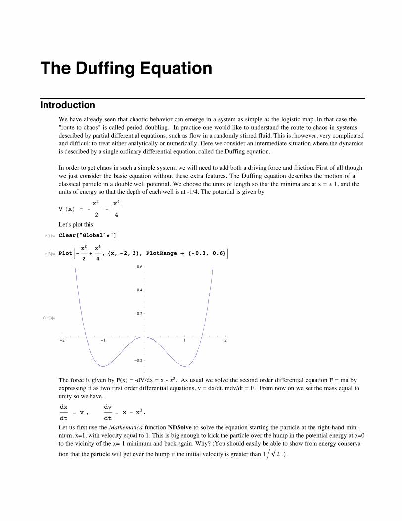
we just consider the basic equation without these extra features. The Duffing equation describes the motion of a
classical particle in a double well potential. We choose the units of length so that the minima are at x = ± 1, and the
units of energy so that the depth of each well is at -1/4. The potential is given by
V HxL = -x2
2+
x4
4
Let's plot this:
In[1]:= Clear@"Global`*"D
In[3]:= PlotB-x2
2+x4
4, 8x, -2, 2<, PlotRange Ø 8-0.3, 0.6<F
Out[3]=
-2 -1 1 2
-0.2
0.2
0.4
0.6
The force is given by F(x) = -dV/dx = x - x3. As usual we solve the second order differential equation F = ma by
expressing it as two first order differential equations, v = dx/dt, mdv/dt = F. From now on we set the mass equal to
unity so we have.
dx
dt= v ,
dv
dt= x - x3.
Let us first use the Mathematica function NDSolve to solve the equation starting the particle at the right-hand mini-
mum, x=1, with velocity equal to 1. This is big enough to kick the particle over the hump in the potential energy at x=0
to the vicinity of the x=-1 minimum and back again. Why? (You should easily be able to show from energy conserva-
tion that the particle will get over the hump if the initial velocity is greater than 1í 2 .)
Page 2
sol1 = NDSolve@ 8v'@tD == x@tD - x@tD^3, x'@tD == v@tD, x@0D == 1,
v@0D == 1<, 8x, v<, 8t, 0, 10< D;
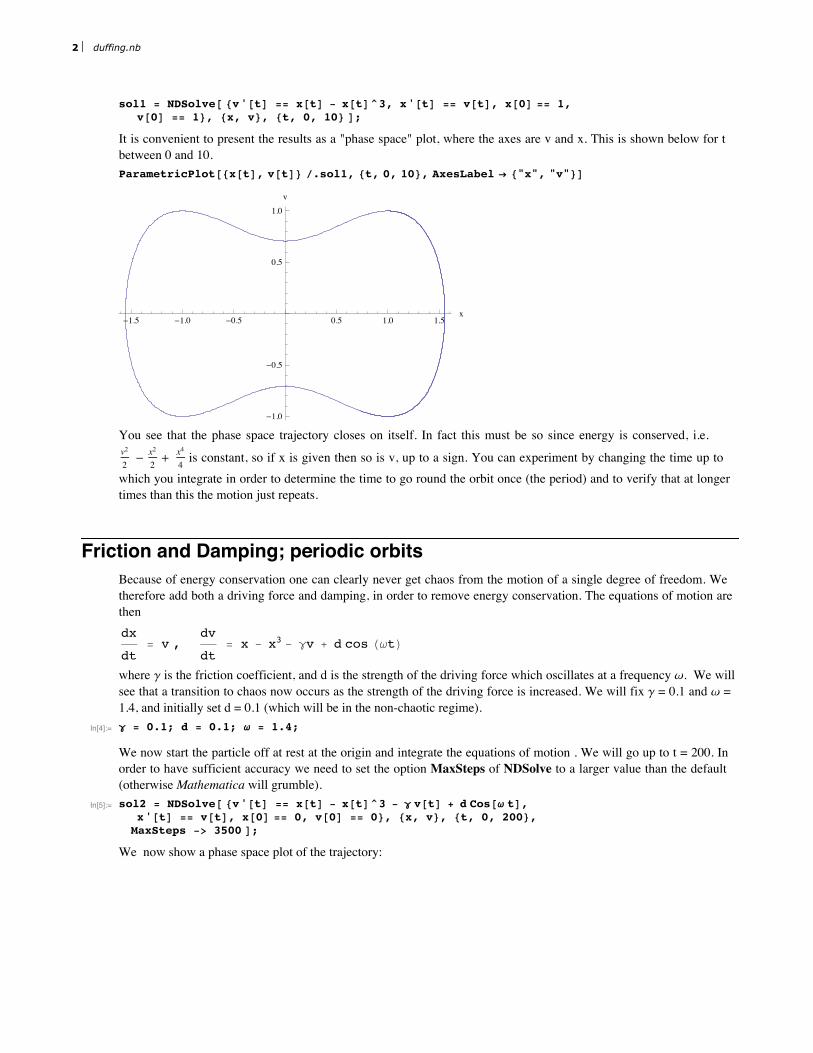
It is convenient to present the results as a "phase space" plot, where the axes are v and x. This is shown below for t
between 0 and 10.
ParametricPlot@8x@tD, v@tD< ê.sol1, 8t, 0, 10<, AxesLabel Ø 8"x", "v"<D
-1.5 -1.0 -0.5 0.5 1.0 1.5x
-1.0
-0.5
0.5
1.0
v
You see that the phase space trajectory closes on itself. In fact this must be so since energy is conserved, i.e.
v2
2-
x2
2+
x4
4is constant, so if x is given then so is v, up to a sign. You can experiment by changing the time up to
which you integrate in order to determine the time to go round the orbit once (the period) and to verify that at longer
times than this the motion just repeats.
Friction and Damping; periodic orbits
Because of energy conservation one can clearly never get chaos from the motion of a single degree of freedom. We
therefore add both a driving force and damping, in order to remove energy conservation. The equations of motion are
then
dx
dt= v ,
dv
dt= x - x3 - gv + d cos HwtL
where g is the friction coefficient, and d is the strength of the driving force which oscillates at a frequency w. We will
see that a transition to chaos now occurs as the strength of the driving force is increased. We will fix g = 0.1 and w =
1.4, and initially set d = 0.1 (which will be in the non-chaotic regime).
In[4]:= g = 0.1; d = 0.1; w = 1.4;
We now start the particle off at rest at the origin and integrate the equations of motion . We will go up to t = 200. In
order to have sufficient accuracy we need to set the option MaxSteps of NDSolve to a larger value than the default
(otherwise Mathematica will grumble).
In[5]:= sol2 = NDSolve@ 8v'@tD == x@tD - x@tD^3 - g v@tD + d Cos@w tD,x'@tD == v@tD, x@0D == 0, v@0D == 0<, 8x, v<, 8t, 0, 200<,MaxSteps -> 3500 D;
We now show a phase space plot of the trajectory:
2 duffing.nb
Page 3
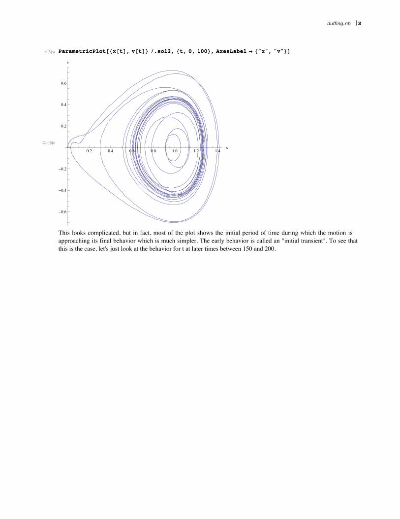
In[6]:= ParametricPlot@8x@tD, v@tD< ê.sol2, 8t, 0, 100<, AxesLabel Ø 8"x", "v"<D
Out[6]=
0.2 0.4 0.6 0.8 1.0 1.2 1.4x
-0.6
-0.4
-0.2
0.2
0.4
0.6
v
This looks complicated, but in fact, most of the plot shows the initial period of time during which the motion is
approaching its final behavior which is much simpler. The early behavior is called an "initial transient". To see that
this is the case, let's just look at the behavior for t at later times between 150 and 200.
duffing.nb 3
Page 4
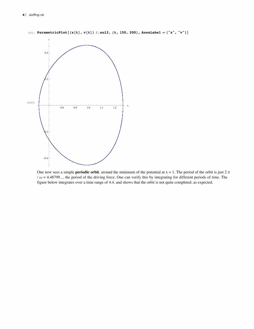
In[7]:= ParametricPlot@8x@tD, v@tD< ê.sol2, 8t, 150, 200<, AxesLabel Ø 8"x", "v"<D
Out[7]=
0.8 0.9 1.0 1.1 1.2x
-0.4
-0.2
0.2
0.4
v
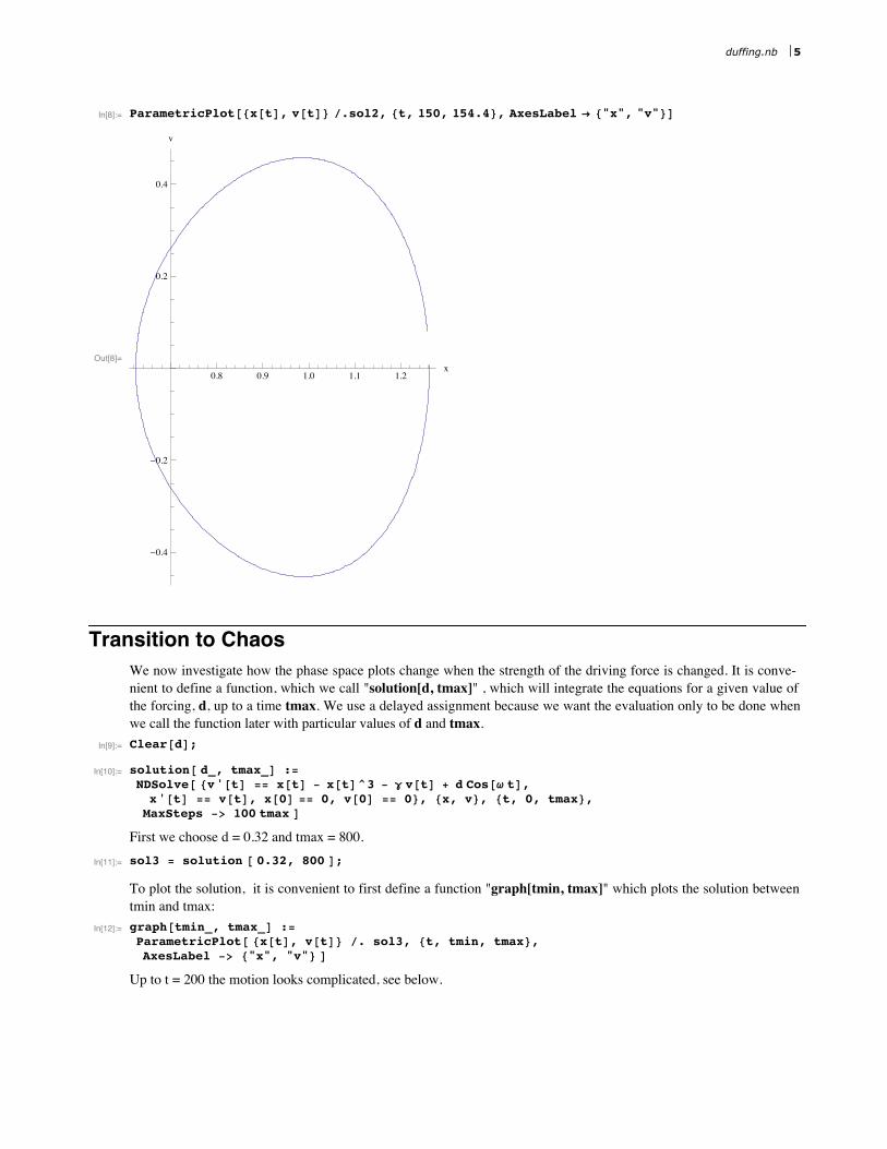
One now sees a simple periodic orbit. around the minimum of the potential at x = 1. The period of the orbit is just 2 p
/ w = 4.48799..., the period of the driving force. One can verify this by integrating for different periods of time. The
figure below integrates over a time range of 4.4, and shows that the orbit is not quite completed, as expected.
4 duffing.nb
Page 5
In[8]:= ParametricPlot@8x@tD, v@tD< ê.sol2, 8t, 150, 154.4<, AxesLabel Ø 8"x", "v"<D
Out[8]=
0.8 0.9 1.0 1.1 1.2x
-0.4
-0.2
0.2
0.4
v
Transition to Chaos
We now investigate how the phase space plots change when the strength of the driving force is changed. It is conve-
nient to define a function, which we call "solution[d, tmax]" , which will integrate the equations for a given value of
the forcing, d, up to a time tmax. We use a delayed assignment because we want the evaluation only to be done when
we call the function later with particular values of d and tmax.
In[9]:= Clear@dD;
In[10]:= solution@ d_, tmax_D :=NDSolve@ 8v'@tD == x@tD - x@tD^3 - g v@tD + d Cos@w tD,x'@tD == v@tD, x@0D == 0, v@0D == 0<, 8x, v<, 8t, 0, tmax<,MaxSteps -> 100 tmax D
First we choose d = 0.32 and tmax = 800.
In[11]:= sol3 = solution @ 0.32, 800 D;
To plot the solution, it is convenient to first define a function "graph[tmin, tmax]" which plots the solution between
tmin and tmax:
In[12]:= graph@tmin_, tmax_D :=ParametricPlot@ 8x@tD, v@tD< ê. sol3, 8t, tmin, tmax<,AxesLabel -> 8"x", "v"< D
Up to t = 200 the motion looks complicated, see below.
duffing.nb 5
Page 6
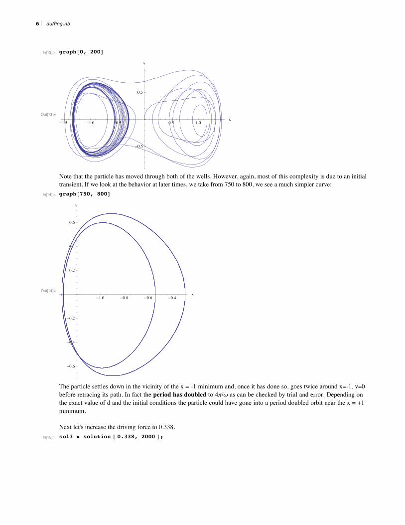
In[13]:= graph@0, 200D
Out[13]=
-1.5 -1.0 -0.5 0.5 1.0x
-0.5
0.5
v
Note that the particle has moved through both of the wells. However, again, most of this complexity is due to an initial
transient. If we look at the behavior at later times, we take from 750 to 800, we see a much simpler curve:
In[14]:= graph@750, 800D
Out[14]=
-1.0 -0.8 -0.6 -0.4x
-0.6
-0.4
-0.2
0.2
0.4
0.6
v
The particle settles down in the vicinity of the x = -1 minimum and, once it has done so, goes twice around x=-1, v=0
before retracing its path. In fact the period has doubled to 4p/w as can be checked by trial and error. Depending on
the exact value of d and the initial conditions the particle could have gone into a period doubled orbit near the x = +1
minimum.
Next let's increase the driving force to 0.338.
In[15]:= sol3 = solution @ 0.338, 2000 D;
6 duffing.nb
Page 7
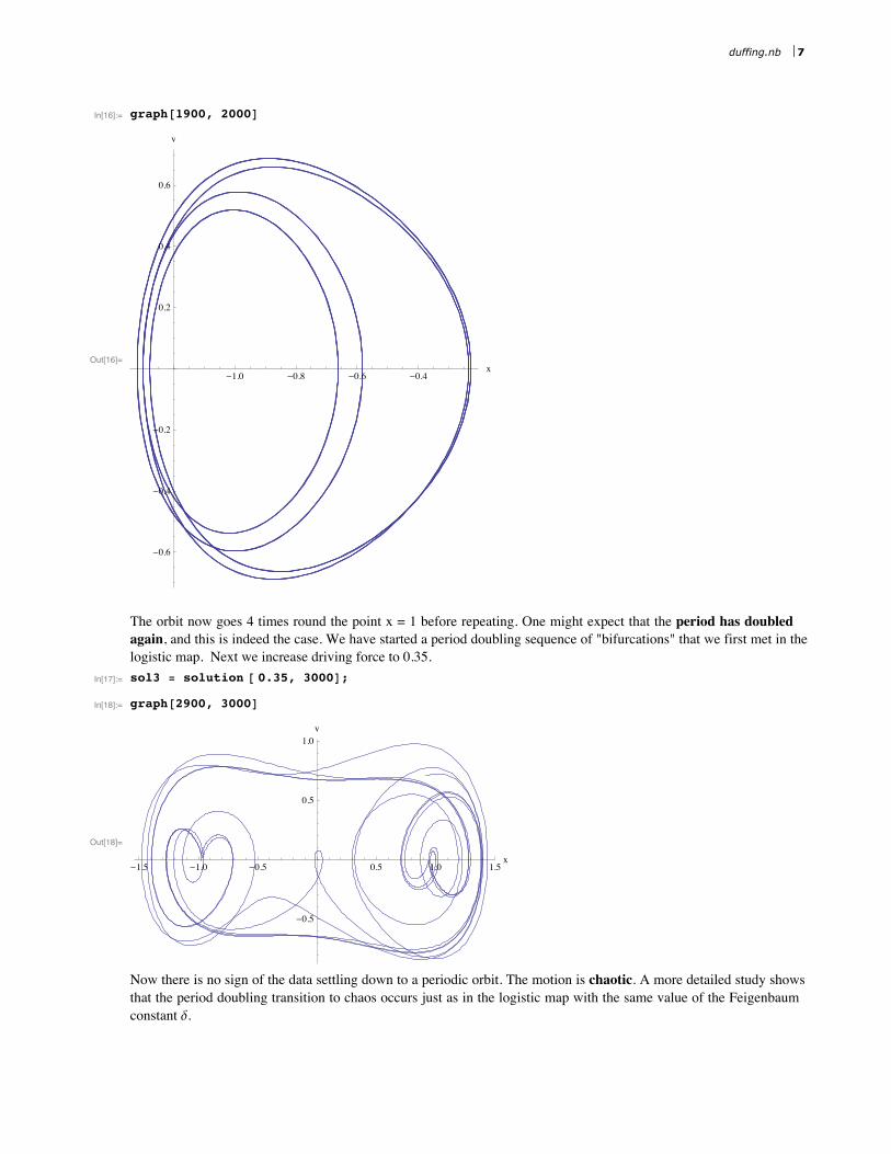
In[16]:= graph@1900, 2000D
Out[16]=
-1.0 -0.8 -0.6 -0.4x
-0.6
-0.4
-0.2
0.2
0.4
0.6
v
The orbit now goes 4 times round the point x = 1 before repeating. One might expect that the period has doubled
again, and this is indeed the case. We have started a period doubling sequence of "bifurcations" that we first met in the
logistic map. Next we increase driving force to 0.35.
In[17]:= sol3 = solution @ 0.35, 3000D;
In[18]:= graph@2900, 3000D
Out[18]=
-1.5 -1.0 -0.5 0.5 1.0 1.5x
-0.5
0.5
1.0
v
Now there is no sign of the data settling down to a periodic orbit. The motion is chaotic. A more detailed study shows
that the period doubling transition to chaos occurs just as in the logistic map with the same value of the Feigenbaum
constant d.
duffing.nb 7
Page 8
Poincaré Sections
A useful way of analyzing chaotic motion is to look at what is called the Poincaré section. Rather than considering the
phase space trajectory for all times, which gives a continuous curve, the Poincaré section is just the discrete set of
phase space points of the particle at every period of the driving force, i.e. at t = 2p/w, 4p/w, 6p/w, etc. Clearly for a
periodic orbit the Poincaré section is a single point, when the period has doubled it consists of two points, and so on.
We define a function, "poincare", which produces a Poincaré section for given values of d, g, and w, in which the first
"ndrop" periods are assumed to be initial transient and so are not plotted, while the subsequent "nplot" periods are
plotted. The point size is given by the parameter "psize".
Note that the function g[{xold, vold}] maps a point in phase space {xold, vold} at time t to the point in phase space {x,
v} one period T later.
This map is then iterated with NestList.
poincare@d_, g_, w_, ndrop_, nplot_, psize_D := HT = 2 p ê w;g@8xold_, vold_<D := 8x@TD, v@TD< ê. NDSolve@8v'@tD ã x@tD - x@tD^3 - g v@tD + d Cos@w tD,
x'@tD ã v@tD, x@0D ã xold, v@0D ã vold<, 8x, v<, 8t, 0, T<D@@1DD;lp = ListPlot@Drop@NestList@g, 80, 0<, nplot + ndropD, ndropD,
PlotStyle Ø 8PointSize@psizeD, Hue@0D<, PlotRange Ø All, AxesLabel Ø 8"x", "v"<DL
If we put in parameters corresponding to a limit cycle of length 4 we get 4 points as expected.
[email protected] , 0.1, 1.4, 1900, 100, 0.02D
-1.26 -1.24 -1.22 -1.20 -1.18 -1.16x
-0.2
0.2
0.4
v
Strange attractor
However,the Poincaré section for parameters in the chaotic regime is much richer. Here we take d = 0.35,
poincare @ 0.35, 0.1, 1.4, 200, 15 000, 0.002D;
The semicolon means that the graphics object lp will not be displayed. It will be plotted in the next command, with
some additional plot options, using Show:
8 duffing.nb
Page 9
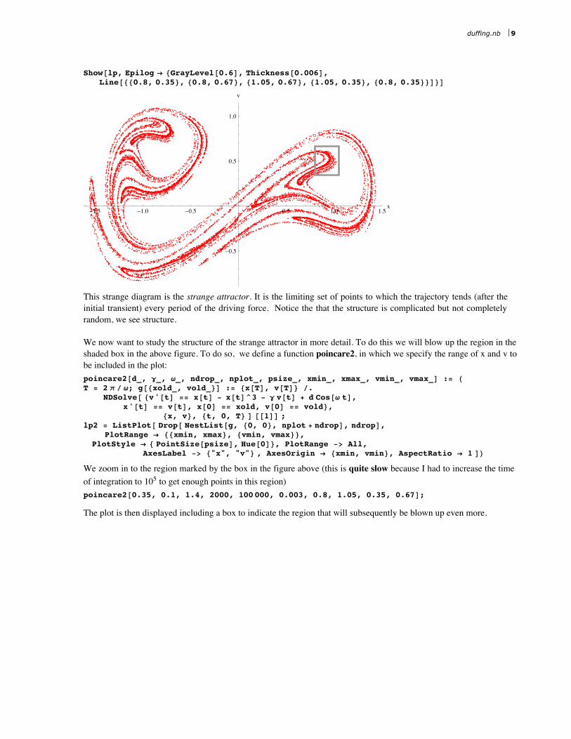
Show@lp, Epilog Ø [email protected] , [email protected] ,[email protected] , 0.35<, 80.8, 0.67<, 81.05, 0.67<, 81.05, 0.35<, 80.8, 0.35<<D<D
-1.5 -1.0 -0.5 0.5 1.0 1.5x
-0.5
0.5
1.0
v
This strange diagram is the strange attractor. It is the limiting set of points to which the trajectory tends (after the
initial transient) every period of the driving force. Notice the that the structure is complicated but not completely
random, we see structure.
We now want to study the structure of the strange attractor in more detail. To do this we will blow up the region in the
shaded box in the above figure. To do so, we define a function poincare2, in which we specify the range of x and v to
be included in the plot:
poincare2@d_, g_, w_, ndrop_, nplot_, psize_, xmin_, xmax_, vmin_, vmax_D := HT = 2 p ê w; g@8xold_, vold_<D := 8x@TD, v@TD< ê.
NDSolve@ 8v'@tD == x@tD - x@tD^3 - g v@tD + d Cos@w tD,x'@tD == v@tD, x@0D == xold, v@0D == vold<,
8x, v<, 8t, 0, T< D @@1DD ;lp2 = ListPlot@ Drop@ NestList@g, 80, 0<, nplot + ndropD, ndropD,
PlotRange Ø 88xmin, xmax<, 8vmin, vmax<<,PlotStyle Ø 8 PointSize@psizeD, Hue@0D<, PlotRange -> All,
AxesLabel -> 8"x", "v"< , AxesOrigin Ø 8xmin, vmin<, AspectRatio Ø 1 DL
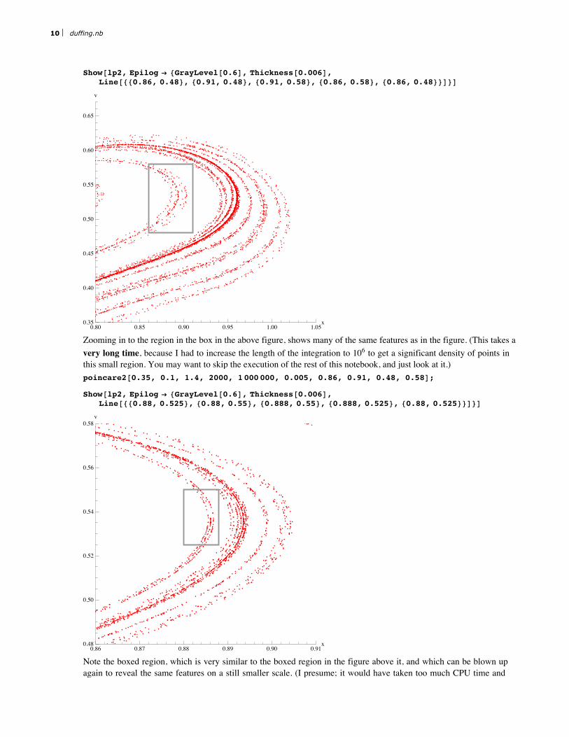
We zoom in to the region marked by the box in the figure above (this is quite slow because I had to increase the time
of integration to 105 to get enough points in this region)
[email protected] , 0.1, 1.4, 2000, 100000, 0.003, 0.8, 1.05, 0.35, 0.67D;
The plot is then displayed including a box to indicate the region that will subsequently be blown up even more.
duffing.nb 9
Page 10
Show@lp2, Epilog Ø [email protected] , [email protected] ,[email protected] , 0.48<, 80.91, 0.48<, 80.91, 0.58<, 80.86, 0.58<, 80.86, 0.48<<D<D
0.80 0.85 0.90 0.95 1.00 1.05x0.35
0.40
0.45
0.50
0.55
0.60
0.65
v
Zooming in to the region in the box in the above figure, shows many of the same features as in the figure. (This takes a
very long time, because I had to increase the length of the integration to 106 to get a significant density of points in
this small region. You may want to skip the execution of the rest of this notebook, and just look at it.)
[email protected] , 0.1, 1.4, 2000, 1000 000, 0.005, 0.86, 0.91, 0.48, 0.58D;
Show@lp2, Epilog Ø [email protected] , [email protected] ,[email protected] , 0.525<, 80.88, 0.55<, 80.888, 0.55<, 80.888, 0.525<, 80.88, 0.525<<D<D
0.86 0.87 0.88 0.89 0.90 0.91x0.48
0.50
0.52
0.54
0.56
0.58
v
Note the boxed region, which is very similar to the boxed region in the figure above it, and which can be blown up
again to reveal the same features on a still smaller scale. (I presume; it would have taken too much CPU time and
memory to check it.)
10 duffing.nb
Page 11
again to reveal the same features on a still smaller scale. (I presume; it would have taken too much CPU time and
memory to check it.)
Having the same features appearing in different parts of a figure and at different scales is a characteristic feature of a
fractal.
Integrating a differential equation, as we have done here, is much more time consuming than iterating a map, such as
the logistic map. People have therefore investigated maps which have similar behavior to that of driven, damped
differential equations like the Duffing equation. One popular choice is the Hénon map:
xn+1 = 1 - a xn2+ yn
yn+1 = b xn
in which two variables, x and y, are iterated. The parameters a and b can be adjusted to get a transition to chaos. In the
chaotic regime the points to converge to a strange attractor similar to the one found for the Duffing equation. Note, in
particular, the way it folds back on itself. A discussion of using Mathematica to display the Hénon map is given in
Zimmerman and Olness, Mathematica for Physics, p. 289.
More on the transition to chaos
Going back to the Duffing equation, you can try different values of the parameters g and w and see where the period
doubling transition to chaos occurs. The function bifurcation below, is similar to poincare except that it scans a range
of values of d, and gives the x-values on the attractor for each d. (It can take a long time to execute).
bifurcation@dmin_, dmax_, nd_, g_, w_, ndrop_, nplot_, psize_D :=
T =2 p
w; g@8xold_, vold_<D :=
8x@TD, v@TD< ê.NDSolveA9v£@tD ã x@tD - x@tD3 - g v@tD + d Cos@w tD, x£@tD ã v@tD,x@0D ã xold, v@0D ã vold=, 8x, v<, 8t, 0, T<EP1T; f@8x_, y_<D := 8d, x<;
ListPlotBFlattenBTableBf êü Drop@NestList@g, 81, 0<, nplot + ndropD, ndropD,
:d, dmin, dmax,dmax - dmin
nd>F, 1F,
PlotStyle Ø 8PointSize@psizeD, Hue@0D<, PlotRange Ø 88dmin, dmax<, 8-1.6, 1.6<<,
AxesLabel Ø 8"d", "x"<, AxesOrigin Ø 8dmin, -1.6<F
The command Flatten[ ... , 1] removes one layer of curly brackets. (Without that we would have separate lists for each
value of d. Flatten[ ... 1] gives us one long list, each element of which is a list comprising a pair of points in (d, x)
space which is to be plotted.) The syntax f /@ list is equivalent to Map[f, list], i.e. apply the function f to each element
of list.
The following command scans 200 values of d in the range from 0.3 to 0.35, with g =0.1 and w =1.4. It starts with v=0
and x=1, i.e.at rest in the x=1 minimum.The equations are integrated for 1500 periods of the driving force with the first
1000 being ignored and the value of x plotted at the end of each of the remaining 500 periods. (This is very slow)
duffing.nb 11
Page 12
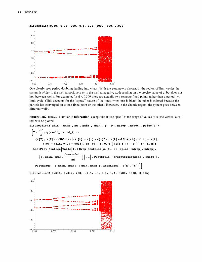
[email protected] , 0.35, 200, 0.1, 1.4, 1000, 500, 0.006D
0.30 0.31 0.32 0.33 0.34 0.35d
-1.5
-1.0
-0.5
0.0
0.5
1.0
1.5
x
One clearly sees period doubling leading into chaos. With the parameters chosen, in the region of limit cycles the
system is either in the well at positive x or in the well at negative x, depending on the precise value of d, but does not
hop between wells. For example, for d < 0.309 there are actually two separate fixed points rather than a period two
limit cycle. (This accounts for the “spotty” nature of the lines, when one is blank the other is colored because the
particle has converged on to one fixed point or the other.) However, in the chaotic region, the system goes between
different wells.
bifurcation2, below, is similar to bifurcation, except that it also specifies the range of values of x (the vertical axis)
that will be plotted.
bifurcation2@dmin_, dmax_, nd_, xmin_, xmax_, g_, w_, ndrop_, nplot_, psize_D :=
T =2 p
w; g@8xold_, vold_<D :=
8x@TD, v@TD< ê.NDSolveA9v£@tD ã x@tD - x@tD3 - g v@tD + d Cos@w tD, x£@tD ã v@tD,x@0D ã xold, v@0D ã vold=, 8x, v<, 8t, 0, T<EP1T; f@8x_, y_<D := 8d, x<;
ListPlotBFlattenBTableBf êü Drop@NestList@g, 81, 0<, nplot + ndropD, ndropD,
:d, dmin, dmax,dmax - dmin
nd>F, 1F, PlotStyle Ø 8PointSize@psizeD, Hue@0D<,
PlotRange Ø 88dmin, dmax<, 8xmin, xmax<<, AxesLabel Ø 8"d", "x"<F
[email protected] , 0.342, 200, -1.5, -1, 0.1, 1.4, 3500, 1000, 0.006D
0.334 0.336 0.338 0.340 0.342d-1.5
-1.4
-1.3
-1.2
-1.1
-1.0
x
12 duffing.nb
Page 13
We have zoomed in to the later stages of the period doubling route to chaos, plotting just the region near the minimum
at negative x.
duffing.nb 13


![Numerical solution of the Duffing equation with random coefficients · 2017. 8. 27. · perature variations as well as shock, impact and fatigue [3, 8] may have a decisive role for](https://static.documents.pub/doc/80x56/60c5cdfa3bbcec27a96f95a9/numerical-solution-of-the-duffing-equation-with-random-coefficients-2017-8-27.jpg)


