ORIGINAL ARTICLE The dynamic redeployment coverage location model Cem Saydam 1 , Hari K. Rajagopalan 2 , Elizabeth Sharer 2 and Kay Lawrimore-Belanger 2 1 Business Information Systems and Operations Management Department, The University of North Carolina at Charlotte, Charlotte, U.S.A.; 2 School of Business, Francis Marion University, Florence, U.S.A. Correspondence: Cem Saydam, Business Information Systems and Operations Management Department, The Belk College of Business, The University of North Carolina at Charlotte, Charlotte, NC, U.S.A. Tel: þ 1 704-687-7616; Fax: þ 1 704-687-6938; E-mail: [email protected]Received: 8 May 2012 Revised: 2 October 2012 2nd Revision: 30 November 2012 Accepted: 10 December 2012 Abstract Demand for ambulances is known to fluctuate spatially and temporally by day of the week and time of day. Faced with fluctuating demand during the day, emergency medical systems (EMS) managers utilize redeployment strategies to meet demand. Such shifting of personnel, although better able to cover a region with fluctuating demand, can cause fatigue amongst ambulance crew members. Considering these phenomena, we extend the dynamic available coverage location model to be driven by two objectives: (1) Minimize the number of ambulances, and (2) Minimize the number of redeployments for a given fleet during a given shift. We develop a heuristic search algorithm and present the comparative statistics using real data from an urban EMS agency. Our findings suggest that EMS managers can effectively balance a need for additional ambulances with those redeployments required to meet variable demand patterns. Health Systems advance online publication 25 January 2013; corrected online 19 February 2013; doi:10.1057/hs.2012.27 Keywords: location models; hypercube; dynamic redeployment; emergency response systems; heuristic search Introduction and motivation Historically, ambulances have been located at fire stations, hospitals and/ or ambulance-specific stations (Goldberg, 2004). As communities realize population growth, demand for ambulance services has grown in parallel, typically requiring the establishment of additional bases. In an effort to assist/inform the making of strategic-level ambulance location (base) deci- sions, researchers developed a variety of static ambulance location models (Brotcorne et al, 2003). As the demand for ambulances fluctuates spatially and temporally by both day-of-the- week and time-of-the-day, the building of permanent (fixed) bases to cover such varying forms of demand is indeed costly and may, in fact, be ineffective. Recent advances in computing, geographic information systems and commercially available software tools (e.g., MARVLIS (Bradshaw Consult- ing Services, 2008), Optima Live (The Optima Corporation, 2012)), as well as the availability of global positioning system signals, have enabled emergency medical systems (EMS) managers to implement redeployment plans (Gendreau et al, 2001; Rajagopalan et al, 2008). Redeployment is defined as moving ambulances from one part of a city to another when faced with a fluctuating demand. There are generally two types of rede- ployment plans: (1) Multi-period and (2) Real-time. The former are created a priori and utilize call volume forecasts for various sectors of a city, and for a few hour-blocks, in order to redeploy a fleet in anticipation of demand shifts in space and magnitude. Under a real-time redeployment plan, when one or more vehicles are dispatched, the remaining available ambulances Health Systems (2013), 1–17 & 2013 Operational Research Society Ltd. All rights reserved 2047-6965/13 www.palgrave-journals.com/hs/
Transcript
ORIGINAL ARTICLE
The dynamic redeployment coverage location
model
Cem Saydam1,Hari K. Rajagopalan2,Elizabeth Sharer2 andKay Lawrimore-Belanger2
1Business Information Systems and Operations
Management Department, The University of
North Carolina at Charlotte, Charlotte, U.S.A.;2School of Business, Francis Marion University,Florence, U.S.A.
Correspondence: Cem Saydam, BusinessInformation Systems and OperationsManagement Department, The Belk Collegeof Business, The University of North Carolinaat Charlotte, Charlotte, NC, U.S.A.Tel: þ1 704-687-7616;Fax: þ1 704-687-6938;E-mail: [email protected]
Received: 8 May 2012Revised: 2 October 20122nd Revision: 30 November 2012Accepted: 10 December 2012
AbstractDemand for ambulances is known to fluctuate spatially and temporally by day of
the week and time of day. Faced with fluctuating demand during the day,
emergency medical systems (EMS) managers utilize redeployment strategies tomeet demand. Such shifting of personnel, although better able to cover a region
with fluctuating demand, can cause fatigue amongst ambulance crew members.
Considering these phenomena, we extend the dynamic available coveragelocation model to be driven by two objectives: (1) Minimize the number of
ambulances, and (2) Minimize the number of redeployments for a given fleet
during a given shift. We develop a heuristic search algorithm and present thecomparative statistics using real data from an urban EMS agency. Our findings
suggest that EMS managers can effectively balance a need for additional
ambulances with those redeployments required to meet variable demand patterns.
Health Systems advance online publication 25 January 2013;corrected online 19 February 2013; doi:10.1057/hs.2012.27
Introduction and motivationHistorically, ambulances have been located at fire stations, hospitals and/or ambulance-specific stations (Goldberg, 2004). As communities realizepopulation growth, demand for ambulance services has grown in parallel,typically requiring the establishment of additional bases. In an effort toassist/inform the making of strategic-level ambulance location (base) deci-sions, researchers developed a variety of static ambulance location models(Brotcorne et al, 2003). As the demand for ambulances fluctuates spatiallyand temporally by both day-of-the- week and time-of-the-day, the buildingof permanent (fixed) bases to cover such varying forms of demand is indeedcostly and may, in fact, be ineffective.
Recent advances in computing, geographic information systems andcommercially available software tools (e.g., MARVLIS (Bradshaw Consult-ing Services, 2008), Optima Live (The Optima Corporation, 2012)), as wellas the availability of global positioning system signals, have enabledemergency medical systems (EMS) managers to implement redeploymentplans (Gendreau et al, 2001; Rajagopalan et al, 2008). Redeployment isdefined as moving ambulances from one part of a city to another whenfaced with a fluctuating demand. There are generally two types of rede-ployment plans: (1) Multi-period and (2) Real-time. The former are createda priori and utilize call volume forecasts for various sectors of a city, and fora few hour-blocks, in order to redeploy a fleet in anticipation of demandshifts in space and magnitude. Under a real-time redeployment plan, whenone or more vehicles are dispatched, the remaining available ambulances
Health Systems (2013), 1–17
& 2013 Operational Research Society Ltd. All rights reserved 2047-6965/13
www.palgrave-journals.com/hs/
are relocated to ensure that the region is covered to thegreatest extent possible. Although this strategy is expec-ted to improve coverage statistics, there is evidence that itcan have counterproductive effects also. As EMS crewmembers typically work long shifts such as 12- or 24 h,the most common shifts offered by North American EMSproviders (Ragone, 2011), real-time redeployments redu-ces rest time during a shift, increases workload and causesfatigue (Bledsoe, 2003; Henderson, 2011; Greene & Wright,2011). Fatigue-related problems cost America an estima-ted US $18 billion a year in terms of lost productivity,whereas fatigue-related drowsiness on the highways con-tributes to more than 1500 fatalities, 100,000 accidentsand 76,000 injuries annually (Caldwell, 2001). Surpris-ingly, only a third of the EMS providers surveyed byGreene & Wright (2011) report a formal policy or plan forfatigue management.
In view of the serious issues with crew fatigue that wehave outlined, if we can reduce the number of redeploy-ments without sacrificing coverage, we would be able, atleast to some extent, to address the problem of ambu-lance crew fatigue. Considering these phenomena, wehere extend the dynamic available coverage locationmodel (DACL) (Rajagopalan et al, 2008) to include real-life operational goals: (1) Minimize the number ofambulances, and (2) Minimize the number of redeploy-ments for a given fleet during a given shift, while meetingcoverage requirements.
We solve our proposed model, Dynamic RedeploymentCoverage Location (DRCL), using a fast meta-heuristicbased on a steepest descent search with emergencyresponse data from Charlotte, N.C. In order to evaluatethe model’s effectiveness, we compare its results withthose generated by the DACL, which uses a redeploymentstrategy to meet coverage requirements while minimizingthe number of servers; however, it does not seek tominimize the number of redeployments.
The remainder of this paper is organized as follows. Inthe section ‘Background and literature review’, we reviewthe relevant literature. In the section ‘The DynamicRedeployment Coverage Location (DRCL) Model’ theDRCL formulation is detailed. The section ‘The DRCLSolution Algorithm’ introduces the search algorithm tobe used in conjunction with the DRCL. Results from thecomputational experiments and application of the modelto the Charlotte-Mecklenburg, NC data are reported inthe section ‘Computational Experiments’, whereas con-clusions and directions for future research are discussedin the section ‘Summary and Conclusions’.
Background and literature reviewThe literature on location models in general andambulance location problems in particular is rich anddiverse. In this regard, we refer the reader to ReVelle et al(2008) for a comprehensive review of location modeling,and to Brotcorne et al’s (2003) and Goldberg’s (2004)reviews of recent developments in ambulance location
problems. The readers can trace earlier developments inSchilling et al (1993) and Owen & Daskin (1998).
Recent developments in coverage modelsThe first wave of published location models weredeterministic in nature (Toregas et al, 1971; Church &ReVelle, 1974), and, thus, did not account for the pro-bability that a particular ambulance might be busy at agiven time. This uncertainty of availability was subse-quently addressed by probabilistic location models. Suchearly models (Daskin, 1983; ReVelle & Hogan, 1989) usedsimplifying assumptions, for example, all vehicles havethe same busy probability while operating independen-tly. In general, these earlier assumptions were not reflec-tive of ‘real world’ conditions where servers cooperatethrough centralized dispatching, and have varying busyprobabilities. Batta et al (1989) and Rajagopalan (2006)showed that using such assumptions in location modelsmay lead to an overestimation of coverage and an under-estimation of the number of servers required.
More recently, in an effort to increase the realism ofprescriptive models by reducing or eliminating simplify-ing assumptions, researchers have begun utilizing thedescriptive hypercube model. Larson’s hypercube model(1974, 1975) represents an important milestone in that itintroduces a spatially distributed queuing framework forfacility location problems (Owen & Daskin, 1998). Thisstructure, and its various extensions, have been foundparticularly useful in determining the performance ofEMS systems (Larson, 1974; Larson & Odoni 1981; Battaet al, 1989; Burwell et al, 1993; Saydam et al, 1994; Daskin,1995; Chan, 2001; Saydam & Aytug, 2003; Goldberg,2004).
Given that the hypercube is computationally expensive,Larson’s approximation (1975) is appropriate for situationsinvolving large numbers of servers. Two assumptions insuch cases are that service times are exponentially distri-buted and mean service times are independent of theserver and the customer. Interestingly, however, data ana-lysis of real EMS systems show that service times aretypically not exponentially distributed, and, instead, areoften bi-modal (Rajagopalan, 2006). Jarvis extendedLarson’s approximation for loss systems (zero queue) byallowing service time distributions to be general type anddependent on both the server and the customer location(Jarvis, 1985). Jarvis used simulation models to test thesensitivity of the results to the shape of the service distri-butions and reported that the approximation procedureproduced statistics that were generally within a few per-cent of true values. Recent computational experimentsreported in the online supplement by Budge et al confir-med Jarvis’ findings that ‘the shape of the service timedistribution beyond its mean has a small impact on steadystate probabilities for loss systems with distinguishableservers’ (Budge et al, 2009).
Common to these models is the assumption of a long-term perspective. Further, hourly and daily fluctuationsin demand are generally not considered. Coverage, rather
The dynamic redeployment coverage location model Cem Saydam et al2
Health Systems
than number of redeployments, is considered the criticalissue.
Redeployment modelsAs shown by Channouf et al (2007) and Setzler et al (2009),EMS demand is not static, but rather fluctuates throughoutthe week, day of the week, and hour by hour within agiven day. Redeployment models consider operational leveldecisions that managers make on a daily or hour-by-hourbasis in an attempt to relocate ambulances in response todemand fluctuations over both time and space. The fewredeployment models currently found in the literature areof two forms: (1) Real-time, where ambulance redeploy-ment is considered with every call and (2) Multi-period,where an ambulance redeployment plan considers anentire day or week based on demand forecasts.
Real-time redeployment models Real-time redeploymentmodels typically relocate ambulances every time one isdispatched, or becomes available for dispatch, with thegoal of providing maximum coverage at all times. One ofthe earliest examples of real time redeployment is thatpresented by Gendreau et al (2001). The objective of theirdynamic double standard formulation at time t (DDSMt )is to maximize backup coverage while minimizing reloca-tion costs.
There are several important considerations embeddedin this model. Although the primary objective is tomaximize the proportion of calls covered by at least twovehicles within a distance threshold, the model penalizes(1) repeated relocation of the same vehicle, (2) longround trips and (3) long trips. The model’s input para-meters are updated each time a call is received andDDSMt is solved.
As pointed out by Gendreau et al (2006), a drawbackwith real-time redeployment algorithms is the need tocompute a new solution whenever a vehicle becomesunavailable. They noted that especially when calls arrivein quick succession, there may not be enough time togenerate a new solution or the solution could beinfeasible. Hence, they developed the Maximal ExpectedCoverage Relocation Problem that generates a prioricompliance table, which lists the best locations forall possible number of available physician vehicles(Gendreau et al, 2006). In the same spirit of this paper,they also included an upper bound on the number ofrelocations but acknowledge that this may adverselyaffect the expected coverage. Similarly, Alanis et al (2012)developed a two-dimensional Markov chain model toevaluate compliance tables and validated it with arealistic simulation model. Encouraged by the model’sfast solution times, the authors show that the model canbe used to select the best or near optimal compliancetable from a set of 100 random tables.
Maxwell et al (2010) developed a novel approximatedynamic programming (ADP) approach for real-timeredeployments decisions. The objective is to maximizethe number of calls reached within a time threshold,
which they measure by the expected number of missedcalls. They show that after an initial training process toobtain an approximated value function, which can bedone offline, the approach is very fast only taking about45 milliseconds per redeployment decision. They con-duct extensive experiments with data from Edmonton,Canada and another much larger city, demonstrating thescalability of the ADP approach and the quality of theprescribed solutions. Recently, Schmid (2012) applied anADP approach to solve the dynamic ambulance reloca-tion and dispatching problem although explicitly con-sidering temporal variations in call volumes and traveltimes. Using data from Vienna, Austria Schmid showedthat the ADP approach outperforms the current practiceof always dispatching the closest ambulance and return-ing to their home bases.
Multi-period redeployment models The earliest multi-period redeployment model was developed by Repede &Bernardo (1994) who extended Daskin’s maximumexpected coverage location model (MEXCLP) (Daskin,1983) to multiple time intervals. In doing so, the authorssought to capture the temporal variations in demand;hence, they termed their model TIMEXCLP. This modelwas incorporated into a decision support system devel-oped for EMS in Louisville, Kentucky. It is important tonote that, TIMEMEXCLP and MEXCLP employ twosimplifying assumptions: (1) Servers operate indepen-dently and (2) All servers have the same busy probability.These assumptions do not reflect the ‘real world’ accura-tely when servers cooperate through centralized dispatch-ing, and they have varying busy probabilities.
More recently, Schmid & Doerner (2010) extendedGendreau et al’s (1997) double standard model from asingle to a multi-period model. They also explicitlyaccounted for time-dependent variations in speed andresulting changes to coverage. Further, vehicles may berelocated with such changes considered in the objectivefunction. Although the concept of double coverage isintended to be an ad hoc method to account for ambu-lance unavailability, it does not specifically take intoaccount ambulance busy probabilities.
Another redeployment model is the dynamic availablecoverage location model (DACL) of Rajagopalan et al(2008). This model seeks to minimize fleet size whilemeeting specified coverage requirements. Its approachincorporates the uncertainty of vehicle availability usingMarianov & ReVelle’s available coverage concept (1996)and uses the Jarvis hypercube approximation (1985) tocalculate vehicle-specific busy probabilities., DACL issolved using tabu search and the solution validated viasimulation. Importantly, the model allows for relocationsbut does not account for relocations in the objective.Erdogan et al (2010) developed a two-stage approach toscheduling ambulance crews to maximize expected cove-rage for a typical planning horizon of one week. Theysolve the ambulance allocation problem for every hour ofthe week and utilize Budge et al’s (2009) approximate
The dynamic redeployment coverage location model Cem Saydam et al 3
Health Systems
hypercube model to compute station-specific busy pro-babilities. The output of this stage becomes the input fortwo crew-scheduling models they propose and show thattheir second approach, which explicitly takes into accounttemporal coverage equity performs well and is tractable.
The principal contribution of the current research isthe Dynamic Redeployment Model (DRCL), proposedbelow, which is a multi-period redeployment model thatextends DACL by simultaneously minimizing both thenumber of servers and redeployments. Like DACL, it usesJarvis’ hypercube approximation to calculate vehicle-specific busy probabilities. Additional contributions arisefrom development of a fast heuristic to solve the problemof interest here. In particular, we show that DRCLmatches, or exceeds, DACL across all key criteria.
The DRCL modelThe DRCL model minimizes both the number of rede-ployments and servers while maintaining overall cover-age requirements. We now proceed to formulate theproposed model in the spirit of these conditions.
Let,
t: be the index of time intervals from 1 to Tn: be the number of nodes in the systemk: be the index of nodes from 1 to ni: be the index of serversmt: be the number of servers at time thk,t: be the fraction of total demand at node k at time tat: be the available coverage requirement at time tct: be the minimum expected coverage requirement at
time tri,t: be the busy probability of a server at node i at time trt: be the average busy probability of servers time tJt: be the set of nodes, which contains servers at time tDk: be the set of nodes within the maximum relocation
of node kxk,tþ : be the number of redeployments moved out of
node (base or post) k at time txk,t� : be the number of redeployments moved into node
(base or post) k at time t
Also let,
Xi;k;t ¼ 1if server i is innode k at time t
0 if not
8<:
Yk;t ¼ 1if node k is covered by at least oneserver with at reliability at time t
0 if not
8<:
And the coverage parameter is:
ai;k ¼ 1if node k is within the distancethreshold of a server at node i
0 if not
8<:
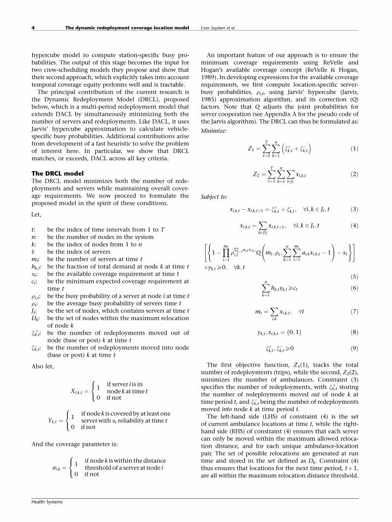
An important feature of our approach is to ensure theminimum coverage requirements using ReVelle andHogan’s available coverage concept (ReVelle & Hogan,1989). In developing expressions for the available coveragerequirements, we first compute location-specific server-busy probabilities, ri,t, using Jarvis’ hypercube (Jarvis,1985) approximation algorithm, and its correction (Q)factors. Note that Q adjusts the joint probabilities forserver cooperation (see Appendix A for the pseudo code ofthe Jarvis algorithm). The DRCL can thus be formulated as:
Minimize:
Z1 ¼XT
t¼2
Xn
k¼1
xþk;t þ x�k;t� �
ð1Þ
Z2 ¼XT
t¼1
Xn
k¼1
Xi2Jt
xi;k;t ð2Þ
Subject to:
xi;k;t � xi;k;tþ1 ¼ xþk;t þ x�k;t ; 8i; k 2 Jt ; t ð3Þ
xi;k;t ¼Xk2Dj
xi;k;tþ1; 8i; k 2 Jt ; t ð4Þ
1�Ymt
i¼1
rSn
k¼1ai;kxi;k;t
i;t Q mt ; rt ;Xn
k¼1
Xmt
i¼1
ai;kxi;k;t � 1
!� at
( )" #
�yk;tX0; 8k; tð5ÞXn
k¼1
hk;tyk;tXct ð6Þ
mt ¼Xi;k
xi;k;t ; 8t ð7Þ
yk;t ; xi;k;t ¼ f0;1g ð8Þ
xþk;t ; x�k;tX0 ð9Þ
The first objective function, Z1(1), tracks the totalnumber of redeployments (trips), while the second, Z2(2),minimizes the number of ambulances. Constraint (3)specifies the number of redeployments, with xk,t
þ storingthe number of redeployments moved out of node k attime period t, and xk,t
� being the number of redeploymentsmoved into node k at time period t.
The left-hand side (LHS) of constraint (4) is the setof current ambulance locations at time t, while the right-hand side (RHS) of constraint (4) ensures that each servercan only be moved within the maximum allowed reloca-tion distance, and for each unique ambulance-locationpair. The set of possible relocations are generated at runtime and stored in the set defined as Dk. Constraint (4)thus ensures that locations for the next time period, tþ1,are all within the maximum relocation distance threshold.
The dynamic redeployment coverage location model Cem Saydam et al4
Health Systems
Constraints (5) ensure that a node is counted only if itcan be covered with reliability at, while constraint (6)requires that all demand covered with reliability at isgreater than or equal to the minimum coverage require-ment, ct. We track the number servers used in t withconstraint (7) and enforce the binary and non-negativityrequirements with constraints (8) and (9), respectively.
The number of servers, mt, is not fixed, but, rather,determined by the algorithm at run time. The model usesa hypercube approximation algorithm to calculate server,hence, location-specific, busy probabilities at run times.Specifically, the parameters (mt, rt, Q) in Eq. (5) arecalculated dynamically at run time.
As a result of the above conditions and constraints, theDRCL model cannot be solved using standard ILP solversbut does lend itself to solution approaches such as meta-heuristic algorithms (Galvao et al, 2005).
The DRCL solution algorithmThe solution algorithm for DRCL has essentially twoobjectives wherein the primary goal is to minimize thenumber of redeployments, while the secondary objectiveis to keep the fleet size at a minimum. Rajagopalan et al(2008) showed that the Reactive Tabu Search (RTS)-basedIncremental Search Algorithm (ISA) used in DACL findsthe minimum number of servers, and their locations,while achieving, or exceeding, coverage requirements.For the first time period, we thus use ISA, and find theminimum fleet size and corresponding server locations.This solution, in turn, becomes the initial solution for thenext time period. In our DRCL model, we take advantageof this high quality initial solution. It is important to
note that ISA is used only to generate the initial solutionfor the first time period. For subsequent time periods, thesearch algorithm described in section 4.2 is used.
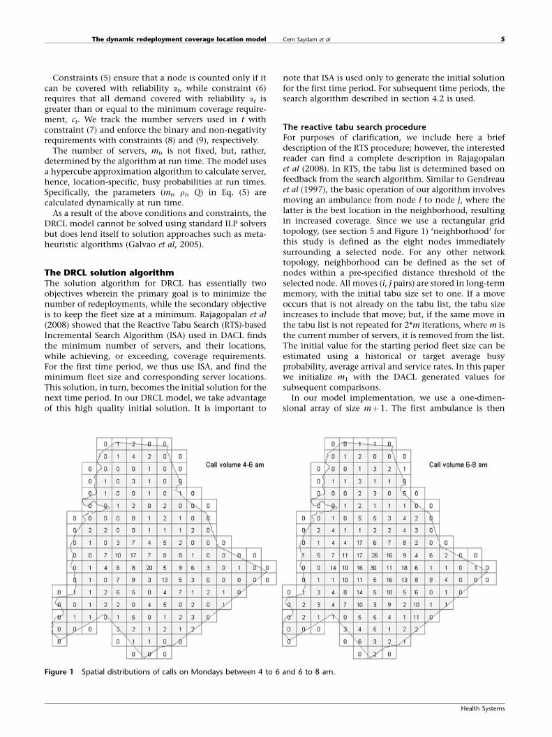
The reactive tabu search procedureFor purposes of clarification, we include here a briefdescription of the RTS procedure; however, the interestedreader can find a complete description in Rajagopalanet al (2008). In RTS, the tabu list is determined based onfeedback from the search algorithm. Similar to Gendreauet al (1997), the basic operation of our algorithm involvesmoving an ambulance from node i to node j, where thelatter is the best location in the neighborhood, resultingin increased coverage. Since we use a rectangular gridtopology, (see section 5 and Figure 1) ‘neighborhood’ forthis study is defined as the eight nodes immediatelysurrounding a selected node. For any other networktopology, neighborhood can be defined as the set ofnodes within a pre-specified distance threshold of theselected node. All moves (i, j pairs) are stored in long-termmemory, with the initial tabu size set to one. If a moveoccurs that is not already on the tabu list, the tabu sizeincreases to include that move; but, if the same move inthe tabu list is not repeated for 2*m iterations, where m isthe current number of servers, it is removed from the list.The initial value for the starting period fleet size can beestimated using a historical or target average busyprobability, average arrival and service rates. In this paperwe initialize m1 with the DACL generated values forsubsequent comparisons.
In our model implementation, we use a one-dimen-sional array of size mþ1. The first ambulance is then
Figure 1 Spatial distributions of calls on Mondays between 4 to 6 and 6 to 8 am.
The dynamic redeployment coverage location model Cem Saydam et al 5
Health Systems
selected for basic operations, and the best node from itsneighborhood is selected only if the pair is not on thetabu list. The best node is selected based on the resultingbest coverage, as given by constraint (3). The pair (i, j)then enters the tabu list. We consider any move toconstitute a single iteration. Subsequently, we system-atically select the next ambulance, and conduct anotherneighborhood search. This process is repeated until allambulances have been selected, after which the firstambulance is selected again.
The stopping criterion for this implementation of RTSis 100 iterations. This number was determined afterrunning a set of sample problems for what we defined asan extensive period of time (1000 iterations, or more).Results from those tests found that incremental gainsafter 100 iterations were negligible. For RTS, the set oflocations generated during the first 100 iterations, whichultimately resulted in maximum coverage, was stored.
Search algorithm for DRCLIn DRCL, as suggested earlier, the initial solution forperiod two is the final solution from period one. Thus,the algorithm first checks if the current solution exceedsthe coverage requirements for t¼2. If so, we conduct asearch to identify which server(s) can be removed with aminimum reduction in coverage. Servers are removeduntil the coverage requirements are no longer met. Theprevious solution that just meets the coverage require-ments is then the new solution for t¼2. Note that, in thisscenario, there is no need to relocate any server(s).
Conversely, if the solution from the previous timeperiod results in coverage that is less than required, then,the algorithm begins with the first server, and searchesfor the best (if any) relocation move within its neighbor-hood that generates the greatest increase (gain) incoverage. Once this location is found, the location isstored in memory with the new coverage value. With thefirst server in the original location, we then search for the‘best’ location for the second server; this location and itscoverage increase are subsequently stored in memory.
This is done for all m servers, resulting in m searches. Theserver that generates the maximum increase in coverageis moved to its new location. Once the server is selectedand moved, that server is placed in a tabu list and cannotbe moved again. If this new configuration of servers doesnot meet the minimum coverage requirement, thealgorithm again searches among the other m�1 serversfor the best one to relocate to a new node.
This process continues until the minimum coveragerequirement is met. The worst case scenario for thisalgorithm would result in m factorial searches. In addi-tion, the algorithm terminates if it finds that it cannotimprove the current coverage by moving any of theavailable servers. The worst case would thus occur only if,at every pass, the algorithm finds a relocation of the lastserver examined that improves its current solution, but,at the same time, does not reach the minimum coveragerequirements. Note that this is a variation of the SteepestDescent Algorithm.
If all possible relocations are explored, and the coveragerequirements are still not met, then, using the most recentsolution with redeployed servers, a search is made for thebest node in order to locate a new server. Servers areincreased until coverage requirements are met. (Full detailsof this algorithm’s flow can be found in Appendix B.)
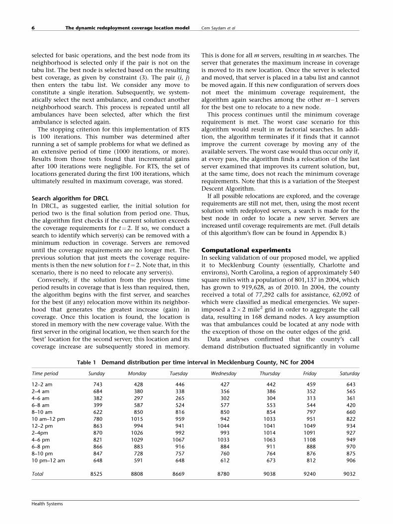
Computational experimentsIn seeking validation of our proposed model, we appliedit to Mecklenburg County (essentially, Charlotte andenvirons), North Carolina, a region of approximately 540square miles with a population of 801,137 in 2004, whichhas grown to 919,628, as of 2010. In 2004, the countyreceived a total of 77,292 calls for assistance, 62,092 ofwhich were classified as medical emergencies. We super-imposed a 2�2 mile2 grid in order to aggregate the calldata, resulting in 168 demand nodes. A key assumptionwas that ambulances could be located at any node withthe exception of those on the outer edges of the grid.
Data analyses confirmed that the county’s calldemand distribution fluctuated significantly in volume
Table 1 Demand distribution per time interval in Mecklenburg County, NC for 2004
Time period Sunday Monday Tuesday Wednesday Thursday Friday Saturday
12–2 am 743 428 446 427 442 459 643
2–4 am 684 380 338 356 386 352 565
4–6 am 382 297 265 302 304 313 361
6–8 am 399 587 524 577 553 544 420
8–10 am 622 850 816 850 854 797 660
10 am–12 pm 780 1015 959 942 1033 951 822
12–2 pm 863 994 941 1044 1041 1049 934
2–4pm 870 1026 992 993 1014 1091 927
4–6 pm 821 1029 1067 1033 1063 1108 949
6–8 pm 866 883 916 884 911 888 970
8–10 pm 847 728 757 760 764 876 875
10 pm–12 am 648 591 648 612 673 812 906
Total 8525 8808 8669 8780 9038 9240 9032
The dynamic redeployment coverage location model Cem Saydam et al6
Health Systems
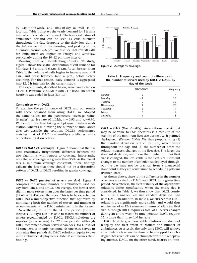
by day-of-the-week, and time-of-day as well as bylocation. Table 1 displays the yearly demand for 2 h timeintervals for each day of the week. The temporal nature ofambulance demand can be seen as calls fluctuatethroughout the day, dropping to the daily low duringthe 4–6 am period in the morning, and peaking in theafternoon around 2–6 pm. We also see that overall callsfor ambulances are higher on Fridays and Saturday,particularly during the 10–12 pm time interval.
Drawing from our Mecklenburg County, NC study,Figure 1 shows the spatial distribution of call demand forMondays 4–6 a.m. and 6 a.m.–8 a.m. As can be seen fromTable 1, the volume of calls begins to increase around 8a.m., and peaks between 4and 6 p.m., before slowlydeclining. For that reason, daily demand is aggregatedinto 12, 2 h intervals for the current study.
The experiments, described below, were conducted ona Dell PC Pentium IV 3.4 MHz with 2 GB RAM. The searchheuristic was coded in Java (jdk 1.4).
Comparison with DACLTo examine the performance of DRCL and our resultswith those obtained from using DACL, we adoptedthe same values for the parameters: coverage radius(6 miles), service rate of 1.02/h, ct¼0.95 and at¼0.90.We demonstrate that taking redeployment into consid-eration, whereas minimizing the number of ambulancesdoes not degrade the solution. DRCL’s performancematches that of DACL on multiple attributes whileoutperforming it on others.
DRCL vs DACL (% coverage) Figure 2 shows that there islittle (statistically insignificant) difference between thetwo algorithms with respect to coverage. Importantly,note that all coverages are greater than 95%. As the modelsets a minimum coverage constraint, these findingsvalidate the fact that there should not be a discerniblepattern of DACL or DRCL resulting in greater coverage.
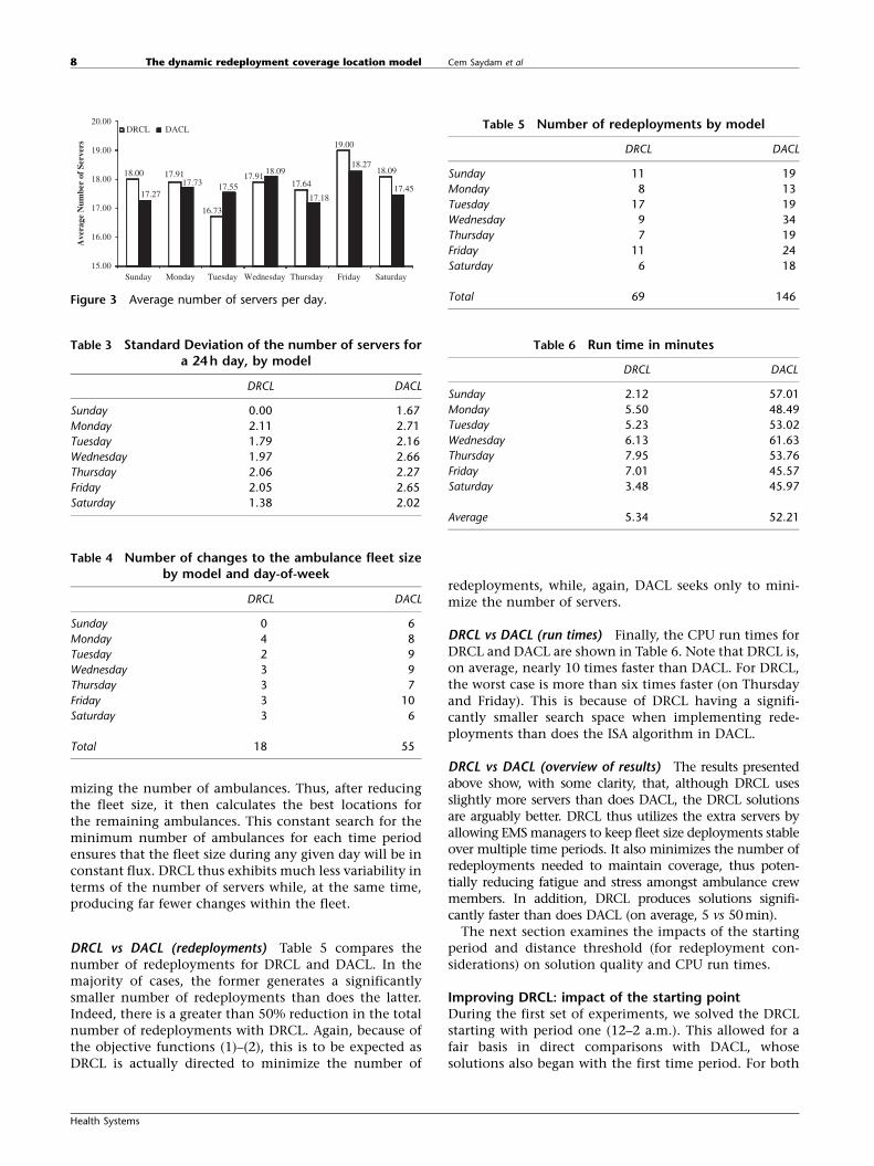
DRCL vs DACL (number of servers per day) Figure 3compares the average number of ambulances used perday from DRCL and DACL. On average, the former usesslightly more servers than does the latter per time period(17.68 vs 17.45) over the week. This is to be expected, asDRCL has a multi-objective function that optimizes byminimizing both the number of servers and number ofredeployments, while DACL minimizes only the former.
Nevertheless, for 30 of the 84 time periods (12 timeintervals�7 days) DRCL is able to match the number ofservers recommended by DACL. DRCL’s solutions aresuperior (fewer servers) for 22 time periods. AlthoughDRCL recommends more servers than does DACL in 20 of32 time periods, it only recommends one extra server. Inonly nine time periods did DRCL solutions require two ormore ambulance deployments. Table 2 summarizes thesefindings.
DRCL vs DACL (fleet stability) An additional metric thatmay be of value to EMS operators is a measure of thestability of the minimum fleet size during a 24 h planneddeployment (Penner, 2004). We thus propose using (1)the standard deviation of the fleet size, which variesthroughout the day, and (2) the number of times thesolution suggests changes in the fleet size. The larger thestandard deviation, and more the number of times fleetsize is changed, the less stable is the fleet size. Constantchanges to the number of ambulances deployed through-out the day may not be practical from a managerialstandpoint as they are constrained by scheduling patterns(Penner, 2004).
As shown above, there is little difference in the numberof servers allocated by DACL and DRCL for a given timeperiod. Nevertheless, the fleet stability of the algorithms’solutions differs significantly when the entire day isconsidered. In Table 3, we thus show that DRCL consis-tently has a smaller fleet size standard deviation thandoes DACL. In addition, in Table 4, we observe that DRCLsolutions are significantly more stable, and would thusrequire less of an EMS manager in terms of adjusting fleetsize. Although DRCL requires a total of 18 server changesduring an entire week (84 time periods), DACL requires55, a more than three-fold increase.
DRCL tends to give more stable solutions as it does notredeploy the fleet when it reduces the number ofambulances. As a result, the only time DRCL will removean ambulance is when the demand has dropped to such adegree that a vehicle can be eliminated without redeploy-ing another. DACL, on the other hand, focuses on mini-
96.39%
95.81%
95.41%
95.83%
96.09%
95.90%
95.78%
96.09%
95.72%95.77% 95.78%
95.55%
96.28%
95.99%
95.00%
95.50%
96.00%
96.50%
Sunday
% C
over
age
DRCL DACL
Monday Tuesday Wednesday Thursday Friday Saturday
Figure 2 Average % coverage.
Table 2 Frequency and count of differences inthe number of servers used by DRCL vs DACL, by
day of the week
DRCL-DACL Frequency
Sunday �2 7
Monday �1 15
Tuesday 0 30
Wednesday 1 20
Thursday 2 9
Friday 3 2
Saturday 4 1
The dynamic redeployment coverage location model Cem Saydam et al 7
Health Systems
mizing the number of ambulances. Thus, after reducingthe fleet size, it then calculates the best locations forthe remaining ambulances. This constant search for theminimum number of ambulances for each time periodensures that the fleet size during any given day will be inconstant flux. DRCL thus exhibits much less variability interms of the number of servers while, at the same time,producing far fewer changes within the fleet.
DRCL vs DACL (redeployments) Table 5 compares thenumber of redeployments for DRCL and DACL. In themajority of cases, the former generates a significantlysmaller number of redeployments than does the latter.Indeed, there is a greater than 50% reduction in the totalnumber of redeployments with DRCL. Again, because ofthe objective functions (1)–(2), this is to be expected asDRCL is actually directed to minimize the number of
redeployments, while, again, DACL seeks only to mini-mize the number of servers.
DRCL vs DACL (run times) Finally, the CPU run times forDRCL and DACL are shown in Table 6. Note that DRCL is,on average, nearly 10 times faster than DACL. For DRCL,the worst case is more than six times faster (on Thursdayand Friday). This is because of DRCL having a signifi-cantly smaller search space when implementing rede-ployments than does the ISA algorithm in DACL.
DRCL vs DACL (overview of results) The results presentedabove show, with some clarity, that, although DRCL usesslightly more servers than does DACL, the DRCL solutionsare arguably better. DRCL thus utilizes the extra servers byallowing EMS managers to keep fleet size deployments stableover multiple time periods. It also minimizes the number ofredeployments needed to maintain coverage, thus poten-tially reducing fatigue and stress amongst ambulance crewmembers. In addition, DRCL produces solutions signifi-cantly faster than does DACL (on average, 5 vs 50min).
The next section examines the impacts of the startingperiod and distance threshold (for redeployment con-siderations) on solution quality and CPU run times.
Improving DRCL: impact of the starting pointDuring the first set of experiments, we solved the DRCLstarting with period one (12–2 a.m.). This allowed for afair basis in direct comparisons with DACL, whosesolutions also began with the first time period. For both
Table 3 Standard Deviation of the number of servers fora 24 h day, by model
DRCL DACL
Sunday 0.00 1.67
Monday 2.11 2.71
Tuesday 1.79 2.16
Wednesday 1.97 2.66
Thursday 2.06 2.27
Friday 2.05 2.65
Saturday 1.38 2.02
Table 4 Number of changes to the ambulance fleet sizeby model and day-of-week
The dynamic redeployment coverage location model Cem Saydam et al8
Health Systems
algorithms, period one could be considered a randomstarting point as it requires neither the least, nor themost, number of servers. DRCL, however, is heavilydependent on the initial solution, and therefore, theinitial time period.
The possibility of obtaining improved solutions bystarting with that time period containing either themaximum or minimum number of servers is explored foreach day. DRCL-H and DRCL-L are used, respectively, torefer to these runs. Table 7 summarizes the starting timeperiod, and the number of servers in each of the threestarting period runs (DRCL, DRCL-H and DRCL-L). (SeeAppendix C for detailed results from all runs.)
Impact of starting point on coverage We first tested todetermine whether the starting point has any impact oncoverage. Figure 4 illustrates that the starting pointappears to have little or no significant impact oncoverage. Further, a single factor ANOVA done on thethree groups shows that there is no statistical differencebetween the average coverage of the three groups(p-value 0.38). While DRCL covered 95.89% of the calls,DRCL-L covered 95.94%, and DRCL-H 96.12%. Of the62,092 calls considered, DRCL covered 59,539 with 90%reliability, whereas DRCL-L and DRCL-H covered 34 and138 additional calls, respectively. These findings suggestthat the starting period does not significantly affectcoverage, nor does it generate excess coverage beyond theminimum requirements of 95%.
Impact of starting point on number of servers deployed -Table 8 lists the average number of servers deployed perday for the three starting period runs. DRCL-H, whichuses the peak time period as the starting point, consis-tently uses, on average, more servers than does DRCL-L orDRCL; 19.62, 18.12, and 17.90, respectively. Examiningthe standard deviations in Table 8, we note that there arefewer fluctuations in the number of servers deployedduring the day for DRCL-H (standard deviation¼1.21)relative to those of DRCL-H and DRCL-L, 1.85 and 1.88,respectively.
To test whether the differences between the threestarting point runs are statistically significant, a singlefactor ANOVA (Table 9) was performed. This table showsthat there are, indeed, statistically significant differencesbetween the three groups. Furthermore, a t-test revealsthat while DRCL-H uses more servers, on average, thando DRCL and DRCL-L, the difference between DRCL andDRCL-L is not statistically significant. Referring to Table 7,we see that the least peak period is always time periodthree, (4–6 a.m.). Server requirements are thus ratherdifferent from time period one (12–2 a.m.), with the onlyexception being Sunday mornings. It is therefore notsurprising that no difference exists between DRCL-L andDRCL with respect to the average number of serverdeployments. DRCL-H starts at peak time periods 7, 8 or 9(i.e., 12–2 p.m., 2–4 p.m., and 4–6 p.m.), and begins witha greater number of servers. Understandably, then, thesolutions recommended by DRCL-H place, on average,one more server than do solutions using the DRCL orDRCL-L approaches.
Impact of starting point on fleet stability Table 10 showsthe range of the number of servers deployed during the
Table 7 Algorithm starting times and the resultingnumber of servers, by day of the week
DRCL DRCL-H DRCL-L
Start
time
Starting
servers
Start
time
Starting
servers
Start
time
Starting
servers
Sunday 1 18 7 20 4 14
Monday 1 13 8 20 3 13
Tuesday 1 14 9 20 3 13
Wednesday 1 15 8 22 3 13
Thursday 1 14 7 20 3 13
Friday 1 16 8 22 3 14
Saturday 1 17 7 20 3 14
95.89%
96.12%95.94%
95.00%
95.50%
96.00%
96.50%
DRCL
% C
over
age
DRCL-H DRCL-L
Figure 4 Average % Coverage by model and starting point.
Table 8 Average number of servers deployed, by modeland day of the week
Between Groups 161.9365 2 80.9682 28.7775 0.0000 3.0321
Within Groups 700.5833 249 2.8135
Total 862.5198 251
The dynamic redeployment coverage location model Cem Saydam et al 9
Health Systems
three starting time period runs. Note that the range forDRCL-H does not vary as much as it does for DRCL andDRCL-L. This is due primarily to the nature of thealgorithm, which focuses on minimizing redeploymentat the expense of minimizing the number of servers.When the algorithm starts with fewer servers, it is forcedto subsequently add them in response to the coverageconstraint (lower bound). However, when it starts withmore servers it subsequently reduces them as long as itdoesn’t necessitate redeployment. If at any point, thenumber of servers cannot be reduced without a redeploy-ment (to maintain coverage), the algorithm maintainsthe current number. This feature results in DRCL-Hrecommending more servers; however, the solutions willbe more stable, thereby avoiding the need to constantlychange fleet size from one time period to another.
Impact of starting point on number of redeployments Aswe continue our analysis of starting points, the numberof redeployments by starting point is compared. Table 11shows that DRCL-H has the least number of redeploy-ments, followed by DRCL-L, and then DRCL. DRCL-H hasthe least number since it uses, on an average, one moreambulance per day. Simply put, using more ambulancesrequires less redeployment. DRCL-L has more redeploy-ments than does DRCL-H, but fewer than DRCL.
Since DRCL-L starts with the period requiring thesmallest number of ambulances, the next time period willrequire more simply ensuring coverage. Since redeploy-ments are restricted to a 3-mile threshold, it is likely thatthe new solution actually adds more servers than needed,and reduces the number of redeployments. This phe-nomenon can, in fact, be seen in Appendix C where thenumber of servers on Monday at time period three(starting time period for DRCL-L) is 13, then jumps to17 in the next time period, and, yet, there are noredeployments. In contrast, DRCL, which starts with ahigher number of servers than DRCL-L, does not go intothe second time period with the minimum number ofservers. As a result, it is able to satisfy the change indemand with redeployment in some cases, and theaddition of servers in others, leading to a greater numberof redeployments overall.
Impact of starting point on run time Finally, Table 12compares the CPU run times for each of the three startingperiods. DRCL-H solves problems fastest (average 2.29min),as it has the smallest changes in the number of servers,and the least number of redeployments. DRCL-L is the nextfastest (average 4.85 min), followed by DRCL (average5.34 min).
From a managerial perspective, we recommend thatdecision-makers run DRCL starting with the peak demandperiod since DRCL-H solves the problem faster, with lessredeployment, and with a more stable configuration ofambulances. A manager cannot, in general, continuouslychange the number of ambulances throughout the day;therefore, stability of this decision variable is a mostimportant consideration. The only drawback we can seeto using DRCL-H is that it will recommend, on average,one extra ambulance be deployed relative to either DRCLor DRCL-L.
Improving DRCL: the impact of distance thresholdThe nature and quality of the solutions generated byDRCL also depend on the distance threshold, which, asnoted earlier, is the maximum distance allowed forambulance relocation. Although the original DRCL hada distance threshold of 3 miles, we used 6 and 9 miles totest the impact of the threshold.
Impact of distance threshold on the average number ofservers Table 13 shows that the average number of
Table 10 Range for number of servers deployed, bymodel and day of the week
Servers Range
DRCL DRCL-H DRCL-L
Sunday 0 1 5
Monday 6 3 8
Tuesday 4 4 7
Wednesday 5 2 6
Thursday 5 3 7
Friday 5 3 5
Saturday 4 2 5
Table 11 Number of redeployments by model and day ofthe week
DRCL DRCL-H DRCL-L
Sunday 11 4 6
Monday 8 4 6
Tuesday 17 3 2
Wednesday 9 9 7
Thursday 7 7 6
Friday 11 1 13
Saturday 6 7 5
Total 69 35 45
Table 12 CPU Run times in minutes by model and day ofthe week
DRCL DRCL-H DRCL-L
Sunday 2.12 1.15 4.53
Monday 5.50 2.46 5.17
Tuesday 5.23 4.56 8.11
Wednesday 6.13 2.34 3.66
Thursday 7.95 2.73 4.58
Friday 7.01 2.44 4.94
Saturday 3.48 0.35 2.97
Total 37.41 16.03 33.96
Average 5.34 2.29 4.85
The dynamic redeployment coverage location model Cem Saydam et al10
Health Systems
recommended servers under a 3-mile-distance thresholdis slightly higher than when the threshold is 6 or 9 miles.
To confirm the existence, or not, of statisticallysignificant differences in the average number of serversby day, a single -factor ANOVA was run with a sample sizeof 84 for each of the three categories (3, 6 and 9 miles).The increase in number of servers required across thethree thresholds was marginal. The results given inTable 14 show that there are no statistically significantdifferences between/amongst these groups.
Impact of distance threshold on number of redeploy-ments We see that in Table 15 the total number ofredeployments increases when the distance thresholdincreases from 3 to 6 miles, and then decreases when thethreshold increases further to 9 miles. There, thus, seemsto be no discernable pattern to the results. For example,there is a significant drop in the number of redeploy-ments when comparing thresholds of 3 and 9 miles onSundays and Tuesdays. However, there is a small drop onFridays, but small increases on Mondays, Thursdays, andSaturdays.
Similarly, in comparing 3 to 6 miles, Mondays andWednesdays have significant increases in the number ofredeployments, whereas Sundays and Saturdays havesmaller increases. At the same time, Thursdays have nochange, but Tuesdays show a significant drop. It can thusbe concluded, but not easily explained, that distancethreshold has little or no clear impact on the number ofredeployments. The changes to redeployment seemrandom. This observation was therefore tested withanother one factor ANOVA (Table 16), which shows that,in fact, there is no significant difference in the number ofredeployments.
Impact of distance threshold on run time Table 17 showsthat using a distance threshold of 3 miles results in CPUrun times that are three to six times faster than thoseusing a distance threshold of nine miles. As the distancethreshold increases, the search space increases, and, so,the run times also increase.
Given. the differences in run time, and the lack ofimprovement in the quality of the solutions when distancethreshold in increased, we conclude that EMS managers aregenerally advised to use the smaller distance threshold ofthree miles.
Summary and conclusions
Cities and counties that locate their ambulances in street
corners and parking lots and redeploy them when the
demand changes achieve greater coverage, but at a certain
cost. (Penner, 2004)
In this paper, we have studied the phenomenon ofambulance redeployment, which improves coverage andresponse time but, at the same time, it can contributeto fatigue within the ambulance crew because of thefrequency of redeployments. In an effort to exploit the
Table 13 Average number of servers deployed per dayfor DRCL
Distance threshold (miles) 3 6 9
Sunday 17.45 16.73 16.73
Monday 16.91 16.55 16.55
Tuesday 15.91 15.82 16.64
Wednesday 16.09 15.82 15.82
Thursday 16.82 15.91 15.91
Friday 17.00 16.91 17.09
Saturday 17.91 17.09 17.09
Average 16.87 16.40 16.55
Table 14 ANOVA Results comparing the average numberof servers across groups
Source of variation SS df MS F P-value F crit
Between Groups 4.95 2 2.48 0.71 0.49 3.03
Within Groups 867.73 249 3.48
Total 872.68 251
Table 15 Total number of redeployments
Distance threshold (miles) 3 6 9
Sunday 11 13 6
Monday 8 13 9
Tuesday 17 7 5
Wednesday 9 16 12
Thursday 7 7 9
Friday 11 9 9
Saturday 6 9 8
Total 69 74 58
Table 16 ANOVA Results comparing the number ofredeployments
Source of variation SS df MS F P-value F crit
Between groups 4.95 2 2.48 0.71 0.49 3.03
Within groups 867.73 249 3.48
Total 872.68 251
Table 17 CPU Run times in minutes for DRCL
Distance threshold (miles) 3 6 9
Sunday 2.12 9.40 14.83
Monday 5.50 13.22 31.69
Tuesday 5.23 13.73 15.99
Wednesday 6.13 14.58 22.43
Thursday 7.95 13.47 27.21
Friday 7.01 13.52 31.37
Saturday 3.48 5.53 22.88
Average 5.34 11.92 23.77
The dynamic redeployment coverage location model Cem Saydam et al 11
Health Systems
advantages of redeployment while mitigating the dis-advantages, we proposed a new, multi-period redeploy-ment model (DRCL) for ambulance location to jointlyminimize the number of planned redeployments andthe fleet size. We then created a solution algorithm tosolve the proposed model, and subsequently comparedsolutions from DRCL to an earlier model (DACL) thatfocused solely on minimizing fleet size.
Our computational experiments show that DRCL,when compared to DACL, reduces the number of rede-ployments by more than half without any significantincrease in fleet size, or reduction in coverage. We alsoshowed that the solutions proposed by DRCL allow fora more stable fleet deployment throughout the day thandoes DACL. This suggests that DRCL would be moreattractive from an EMS manager’s point of view. Further,DRCL algorithms solve empirical problems in 10% of thetime needed for DACL, making it a clearly superioralternative solution methodology for EMS managers.
To further improve DRCL, we examined the effect ofits starting time period to the quality of its solutionand found that starting the model at that time periodcontaining peak demand (DRCL-H) for a given daysignificantly improves the quality of solution; that is tosay, outcomes include fewer redeployments, a smallerstandard deviation to the number of servers deployed,and faster CPU run times. It was also shown that
increasing the distance threshold does not measurablyimprove the solution quality, but does require a longerCPU run time.
There are some limitations of this study thatare important to acknowledge. First, because of thenature of the problem we are constrained to use meta-heuristics. The solutions are therefore not guaranteed tobe optimal. We however have a basis to compare it witha previous method and show that this method worksbetter. Second, we are using Jarvis’ hypercube approx-imation approach to estimate the steady-state individualbusy probabilities, which implicitly overlooks the tran-sient effects. We also have to make certain assumptionswhich further reduce realism. For example, an ambu-lance cannot be intercepted after finishing a call andcoming back to its original position and sent to a newcall. We also assumed that there is only one type ofambulance and the nearest available ambulance dis-patch policy. Future research, using simulation could beused to address these issues and create a more realisticscenario (McLay, 2009).
AcknowledgementsThe authors are indebted to the Editors Professor Harperand Dr. Knight, and the two anonymous referees for their
helpful comments which led to substantial improvements in
this paper.
ReferencesALANIS R, INGOLFSSON A and KOLFAL B (2012) A Markov chain model for an
EMS system with repositioning. Production and Operations Management,doi: I0.1111/j.1937.5956.2012.01362.x
BATTA R, DOLAN JM and KRISHNAMURTHY NN (1989) The maximal expectedcovering location problem: revisited. Transportation Science 23(4),277–287.
BROTCORNE L, LAPORTE G and SEMET F (2003) Ambulance location and reloc-ation models. European Journal of Operational Research 147(3), 451–463.
BUDGE S, INGOLFSSON A and ERKUT E (2009) Approximating vehicledispatch probabilities for emergency service systems with location-specific service times and multiple units per location. Operations Research57(1), 251–255.
BURWELL T, JARVIS JP and MCKNEW MA (1993) Modeling co-located serversand dispatch ties in the hypercube model. Computers & OperationsResearch 20(2), 113–119.
CALDWELL JA (2001) The impact of fatigue in air medical and other typesof operations: a review of fatigue facts and potential countermeasures.Air Medical Journal 20(1), 25–32.
CHAN Y (2001) Location Theory and Decision Analysis. South WesternCollege Publishing, Cincinnati.
CHANNOUF N, L’ECUYER P, INGOLFSSON A and AVRAMIDIS A (2007) The appli-cation of forecasting techniques to modeling emergency medical systemcalls in Calgary, Alberta. Health Care Management Science 10(1), 25–45.
CHURCH RL and REVELLE C (1974) The maximal covering location problem.Papers of Regional Science 32(1), 101–118.
DASKIN MS (1983) A maximal expected covering location model:formulation, properties, and heuristic solution. Transportation Science17(1), 48–69.
DASKIN MS (1995) Network and Discrete Location. John Wiley & Sons Inc.,New York.
ERDOGAN G, ERKUT E, INGOLFSSON A and LAPORTE G (2010) Schedulingambulance crews for maximum coverage. Journal of OperationalResearch Society 61(4), 543–550.
GALVAO RD, CHIYOSHI FY and MORABITO R (2005) Towards unifiedformulations and extensions of two classical probabilistic locationmodels. Computers & Operations Research 32(1), 15–33.
GENDREAU M, LAPORTE G and SEMET F (1997) Solving an ambulancelocation model by Tabu search. Location Science 5(2), 75–88.
GENDREAU M, LAPORTE G and SEMET F (2001) A dynamic model andparallel Tabu search heuristic for real time ambulance relocation.Parallel Computing 27(12), 1641–1653.
GENDREAU M, LAPORTE G and SEMET F (2006) The maximal expectedcoverage relocation problem for emergency vehicles. The Journal of theOperational Research Society 57(1), 22–28.
GOLDBERG JB (2004) Operations research models for the deploymentof emergency services vehicles. EMS Management Journal 1(1), 20–39.
GREENE M and WRIGHT D (2011) Employees seek stability in unstablemarket. Journal of Emergency Medical Services 36(10), 42–49.
HENDERSON SG (2011) Operations research tools for addressing currentchallenges in emergency medical services. In Wiley Encyclopedia ofOperations Research and Management Science. (JJ COCHRAN Ed), JohnWiley & Sons, Inc, Hoboken, NJ.
JARVIS JP (1985) Approximating the equilibrium behavior of multi-serverloss systems. Management Science 31(2), 235–239.
LARSON RC (1974) A hypercube queuing model for facility location andredistricting in urban emergency services. Computers & OperationsResearch 1(1), 67–95.
LARSON RC (1975) Approximating the performance of urban emergencyservice systems. Operations Research 23(5), 845–868.
LARSON RC and ODONI AR (1981) Urban Operations Research. Prentice-Hall, Englewood Cliffs, N.J.
MARIANOV V and REVELLE C (1996) The queueing maximal availabilitylocation problem: a model for siting of emergency vehicles. EuropeanJournal of Operational Research 93(1), 110–120.
The dynamic redeployment coverage location model Cem Saydam et al12
Health Systems
MAXWELL MS, RESTREPO M, HENDERSON SG and TOPALOGLU H (2010)Approximate dynamic programming for ambulance redeployment.INFORMS Journal on Computing 22(2), 266–281.
MCLAY LA (2009) A maximum expected covering location model withtwo types of servers. IIE Transactions 41(8), 730–741.
OWEN SH and DASKIN MS (1998) Strategic facility location: a review.European Journal of Operational Research 111(3), 423–447.
PENNER J (2004) Interview with the Charlotte MEDIC director.H.K. Rajagopalan. Charlotte.
RAGONE MG (2011) Are we ready for the future? Where EMS stands now& where it’s prepared to go. Journal of Emergency Medical Services36(2), 38–43.
RAJAGOPALAN HK (2006) Developing and validating realistic dynamicrelocation models for emergency medical systems: a hybrid meta-heuristic approach. Business Information Systems and OperationsManagement Department. Charlotte, University of North Carolina atCharlotte. Ph.D: 160.
RAJAGOPALAN HK, SAYDAM C and XIAO J (2008) A multiperiod set coveringlocation model for dynamic redeployment of ambulances. Computers& Operations Research 35(3), 814–826.
REPEDE J and BERNARDO J (1994) Developing and validating adecision support system for locating emergency medical vehichlesin Lousville, Kentucky. European Journal of Operational Research75(3), 567–581.
REVELLE C, EISELT HA and DASKIN MS (2008) A bibliography for somefundamental problem categories in discrete location science. EuropeanJournal of Operational Research 184(3), 817–848.
REVELLE C and HOGAN K (1989) The maximum availability locationproblem. Transportation Science 23(3), 192–200.
SAYDAM C and AYTUG H (2003) Accurate estimation of expected cove-rage: revisited. Socio-Economic Planning Sciences 37(1), 69–80.
SAYDAM C, REPEDE J and BURWELL T (1994) Accurate estimation of expectedcoverage: a comparative study. Socio-Economic Planning Sciences28(2), 113–120.
SCHILLING DA, JAYARAMAN V and BARKHI R (1993) A review of coveringproblems in facility location. Location Science 1(1), 25–55.
SCHMID V (2012) Solving the dynamic ambulance relocation anddispatching problem using approximate dynamic programming.European Journal of Operational Research 219(3), 611–621.
SCHMID V and DOERNER KF (2010) Ambulance location and relocationproblems with time-dependent travel times. European Journal ofOperational Research 207(3), 1293–1303.
SETZLER H, SAYDAM C and PARK S (2009) EMS call volume predictions: acomparative study. Computers & Operations Research 36(6), 1843–1851.
THE OPTIMA CORPORATION (2012) Optima Live. The Optima Corporation,Auckland, New Zealand.
TOREGAS C, SWAIN R, REVELLE C and BERGMAN L (1971) The locationof emergency service facilities. Operations Research 19(6), 1363–1373.
CorrectionSince the article was first published the author has noted that in the coverage parameter and in equation 5 in the DRCL model
section, incorrect notation was used. These have been corrected in this final version.
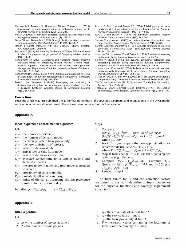
Appendix A
Jarvis’ hypercube approximation algorithm
Let,
m¼ the number of servers,n¼ the number of demand nodes,r¼ the average system busy probability,ri¼ the busy probability of server i,l¼ system wide arrival rate,lj¼ arrival rate of calls from node j,t¼ system wide mean service time,ti,j¼ expected service time for a unit at node i and
demand at node jfij¼ the probability that demand from node j is assigned
to server i,P0¼ probability all servers are idle,Pm¼ probability all servers are busy,ajk¼ index of the server occupying the kth preference
position for calls from node j
Initialize: ri ¼ Sj:aj1¼iljtij t ¼ SNj¼1ðlj=lÞtaj1;j
Steps:
1. ComputeQ(m,r,j)¼
Pk¼ jm�1((m�j�1)!(m�k)(mk)(rk�j)P0)/
(k�j)!(1�Pm)jm!(1�r(1�Pm)) for k¼0,1,y, m�1where r¼ lt/m
2. For i¼1,y, m compute the new approximation forserver workloads, ri(new)¼ (Vi)/(1þVi)where Vi ¼ Sm
k¼1Sj:ajk¼iljtijQ m; r; k� 1ð ÞPk�1l¼1 rajl
3. Stop if max change in ri is less than convergencecriterion (e.g., 1%), else
4. Compute Pm¼1�(P
i¼ 1m ri)/mr, Compute fij ¼
Qðm; r; k� 1Þð1� riÞPk�1l¼1 rajl
; 8i; j; and t¼P
j¼1N (lj/
l)[P
i¼1m tijfij/(1�Pm)]
5. Return to step 1.
The final values for ri and the correction factorsare passed to the main algorithm as input parametersfor the objective functions and coverage requirementconstraints.
Appendix B
DRCL algorithm
Let,
1. mt¼ the number of servers at time t.2. T¼ the number of time periods.
3. lt¼ the arrival rate of calls at time t.4. mt¼ the service rate at time t.5. rt¼ the busy probability at time t.6. Vt¼ the search vector containing the locations of
servers and the coverage at time t.
The dynamic redeployment coverage location model Cem Saydam et al 13
Health Systems
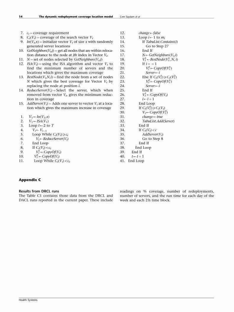
7. ct¼ coverage requirement8. Ct(Vt)¼ coverage of the search vector Vt
9. In(Vt,x)¼ initialize vector Vt of size x with randomlygenerated server locations
10. GetNeighbors(Vt,j)¼ get all nodes that are within reloca-tion distance to the node at jth index in Vector Vt.
11. N¼ set of nodes selected by GetNeighbors(Vt,j)12. ISA(Vt)¼using the ISA algorithm and vector Vt to
find the minimum number of servers and thelocations which gives the maximum coverage
13. BestNode(Vt,N,i)¼ find the node from a set of nodesN which gives the best coverage for Vector Vt byreplacing the node at position i.
14. ReduceServer(Vt)¼ Select the server, which whenremoved from vector Vt, gives the minimum reduc-tion in coverage
15. AddServer(Vt)¼Adds one server to vector Vt at a loca-tion which gives the maximum increase in coverage
1. V1’In(V1,x)2. V1’ISA(V1)3. Loop t’2 to T4. Vt’Vt�1
5. Loop While Ct(Vt)Xct
6. Vt’ReduceServer(Vt)7. End Loop8. If Ct(Vt)oct
9. Vt1’CopyOf(Vt)
10. Vt2’CopyOf(Vt)
11. Loop While Ct(Vt)oct
12. change’false13. Loop i’1 to mt
14. If TabuList.Contains(i)15. Go to Step 2716. End If17. N’GetNeighbors(Vt,i)18. Vt
1’BestNode(Vt1, N, i)
19. If i¼ ¼120. Vt
2’CopyOf(Vt1)
21. Server’i22. Else If Ct(Vt
1)XCt(Vt2)
23. Vt2’CopyOf(Vt
1)24. Server’i25. End If26. Vt
1’CopyOf(Vt)27. i’iþ128. End Loop29. If Ct(Vt
2)XCt(Vt)30. Vt’CopyOf(Vt
2)31. change’true32. TabuList.Add(Server)33. End If34. If Ct(Vt)oc35. AddServer(Vt)36. Go to Step 837. End If38. End Loop39. End If40. t’tþ141. End Loop
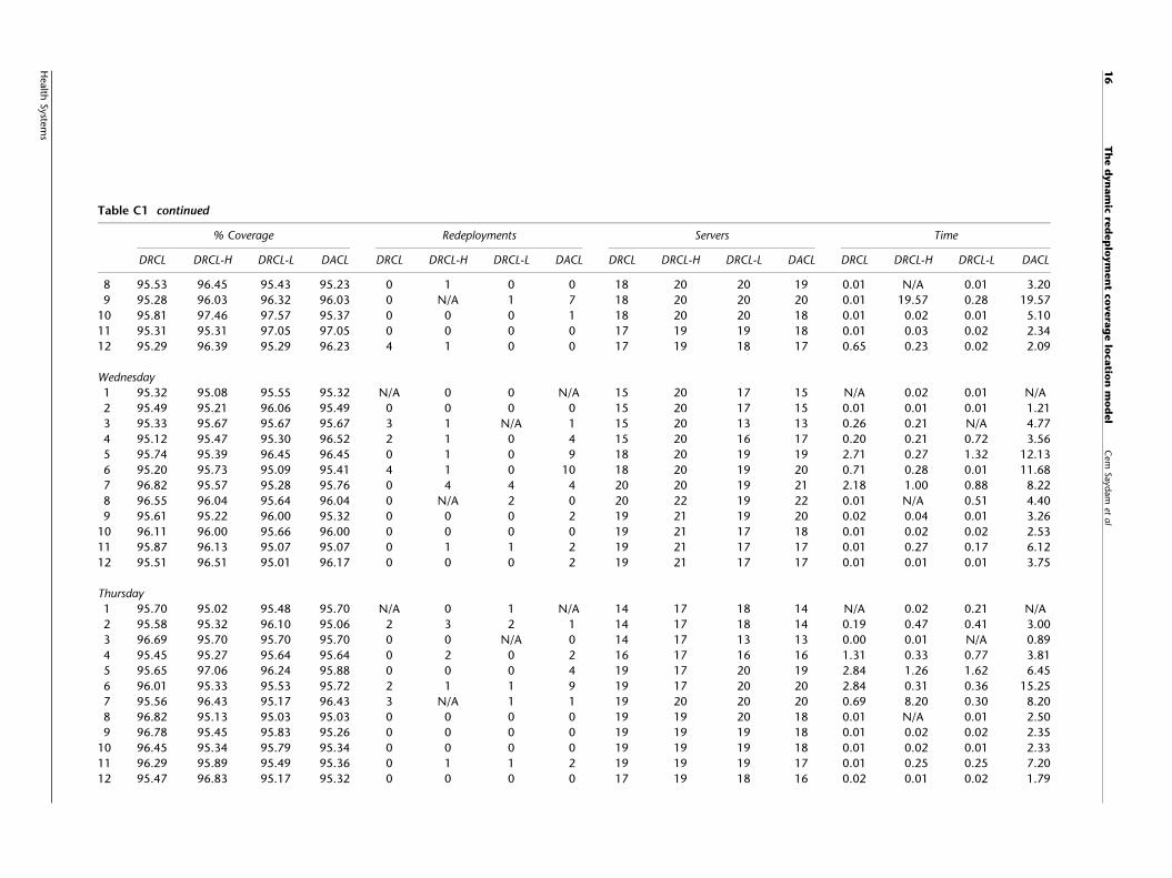
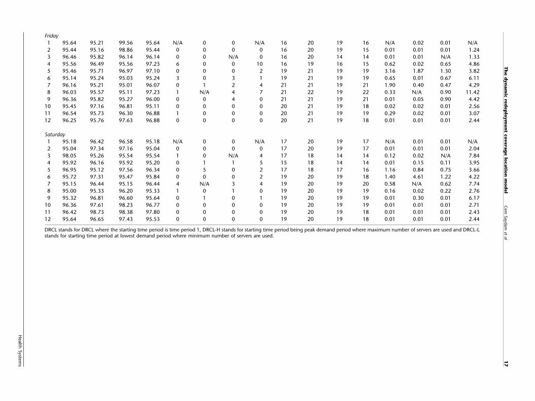
Appendix C
Results from DRCL runsThe Table C1 contains those data from the DRCL andDACL runs reported in the current paper. These include
readings on % coverage, number of redeployments,number of servers, and the run time for each day of theweek and each 2 h time block.
The dynamic redeployment coverage location model Cem Saydam et al14
DRCL stands for DRCL where the starting time period is time period 1, DRCL-H stands for starting time period being peak demand period where maximum number of servers are used and DRCL-Lstands for starting time period at lowest demand period where minimum number of servers are used.