Finance and Economics Discussion Series Divisions of Research & Statistics and Monetary Affairs Federal Reserve Board, Washington, D.C. The Dynamics of Adjustable-Rate Subprime Mortgage Default: A Structural Estimation Hanming Fang, You Suk Kim, and Wenli Li 2015-114 Please cite this paper as: Fang, Hanming, You Suk Kim, and Wenli Li (2015). “The Dynamics of Adjustable-Rate Subprime Mortgage Default: A Structural Estimation,” Finance and Economics Discus- sion Series 2015-114. Washington: Board of Governors of the Federal Reserve System, http://dx.doi.org/10.17016/FEDS.2015.114. NOTE: Staff working papers in the Finance and Economics Discussion Series (FEDS) are preliminary materials circulated to stimulate discussion and critical comment. The analysis and conclusions set forth are those of the authors and do not indicate concurrence by other members of the research staff or the Board of Governors. References in publications to the Finance and Economics Discussion Series (other than acknowledgement) should be cleared with the author(s) to protect the tentative character of these papers.
Transcript
Finance and Economics Discussion SeriesDivisions of Research & Statistics and Monetary Affairs
Federal Reserve Board, Washington, D.C.
The Dynamics of Adjustable-Rate Subprime Mortgage Default: AStructural Estimation
Hanming Fang, You Suk Kim, and Wenli Li
2015-114
Please cite this paper as:Fang, Hanming, You Suk Kim, and Wenli Li (2015). “The Dynamics of Adjustable-RateSubprime Mortgage Default: A Structural Estimation,” Finance and Economics Discus-sion Series 2015-114. Washington: Board of Governors of the Federal Reserve System,http://dx.doi.org/10.17016/FEDS.2015.114.
NOTE: Staff working papers in the Finance and Economics Discussion Series (FEDS) are preliminarymaterials circulated to stimulate discussion and critical comment. The analysis and conclusions set forthare those of the authors and do not indicate concurrence by other members of the research staff or theBoard of Governors. References in publications to the Finance and Economics Discussion Series (other thanacknowledgement) should be cleared with the author(s) to protect the tentative character of these papers.
The Dynamics of Adjustable-Rate Subprime Mortgage Default:
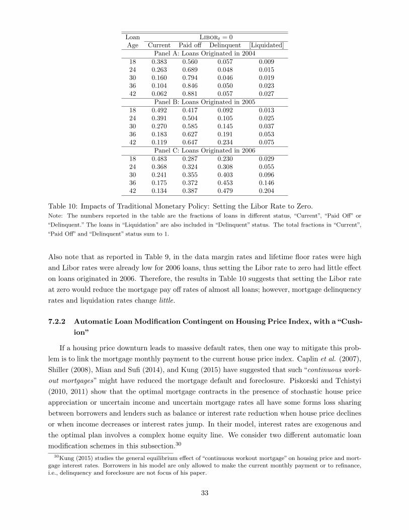
A Structural Estimation∗
Hanming Fang† You Suk Kim‡ Wenli Li§
December 9, 2015
Abstract
We present a dynamic structural model of subprime adjustable-rate mortgage (ARM) bor-
rowers making payment decisions taking into account possible consequences of different degrees
of delinquency from their lenders. We empirically implement the model using unique data sets
that contain information on borrowers’ mortgage payment history, their broad balance sheets,
and lender responses. Our investigation of the factors that drive borrowers’ decisions reveals
that subprime ARMs are not all alike. For loans originated in 2004 and 2005, the interest rate
resets associated with ARMs, as well as the housing and labor market conditions were not as
important in borrowers’ delinquency decisions as in their decisions to pay off their loans. For
loans originated in 2006, interest rate resets, housing price declines, and worsening labor market
conditions all contributed importantly to their high delinquency rates. Counterfactual policy
simulations reveal that even if the Libor rate could be lowered to zero by aggressive traditional
monetary policies, it would have a limited effect on reducing the delinquency rates. We find
that automatic modification mortgage designs under which the monthly payment or the princi-
pal balance of the loans are automatically reduced when housing prices decline can be effective
in reducing both delinquency and foreclosure. Importantly, we find that automatic modification
mortgages with a cushion, under which the monthly payment or principal balance reductions are
triggered only when housing price declines exceed a certain percentage may result in a Pareto
improvement in that borrowers and lenders are both made better off than under the baseline,
with a lower delinquency and foreclosure rates. Our counterfactual analysis also suggests that
limited commitment power on the part of the lenders to loan modification policies may be an
important reason for the relatively small rate of modifications observed during the housing crisis.
∗We thank Shane Sherlund and seminar/conference participants at the Econometric Society World Congress
(2015), University of New South Wales and University of Technology Sydney for their comments. The views expressed
are those of the authors and do not necessarily reflect those of the Board of Governors of the Federal Reserve, the
Federal Reserve Bank of Philadelphia, or the Federal Reserve System.†Department of Economics, University of Pennsylvania, 3718 Locust Walk, Philadelphia, PA 19104 and the NBER.
Email: [email protected].‡Division of Research and Statistics, Board of Governors of the Federal Reserve System. Email: [email protected].§Department of Research, Federal Reserve Bank of Philadelphia. Email: [email protected].
1 Introduction
The collapse of the subprime residential mortgage market played a crucial role in the recent
housing crisis that subsequently led to the Great Recession.1 At the end of 2007, subprime mort-
gages accounted for about 13 percent of all outstanding first-lien residential mortgages but over
half of the foreclosures. The majority of the subprime mortgages, both by number and by value,
were adjustable interest rates mortgages (ARMs); and these mortgages had a foreclosure rate of
17 percent, much higher than the 5 percent foreclosure rate for the fixed-rate subprime mortgages
(Frame, Lehnert, and Prescott 2008, Table 1). In response to these developments, many govern-
ment policies were designed and implemented to change the default incentives of the subprime ARM
borrowers.2 Few structural models, however, exist that can guide us in these efforts, and that can
help us understand why most of the programs had limited success.3
In this paper, we develop a dynamic structural model to study the incentives of the adjustable-
rate subprime borrowers to default, and investigate how these incentives change under various
policies. In our model, at each period, a borrower decides whether to pay the amount due (and
be current) or not pay (and stay in various delinquent status), taking into account the lender’s
responses such as mortgage modification, liquidation, or waiting (i.e., doing nothing). Relative to
the existing structural models on mortgage defaults which we review below, our model has two key
distinguishing features: first, in our model default is not the terminal and absorbing state as we
allow borrowers to self cure their delinquency; second, we consider loan modification as one of the
lenders’ loss mitigation practices while the existing models only allow for liquidation.
We empirically implement our model using unique mortgage loan level data sets that contain
not only detailed information on borrowers’ mortgage payment history and lenders’ responses, but
also credit bureau information about borrowers’ broader balance sheet. We are thus one of the first
to utilize borrowers’ credit bureau information to understand their mortgage payment decisions.4
To track movements in the local housing and labor markets, we further merge our data with zip
code level home price indices and county level unemployment rates.
1There is no standard definition of subprime mortgage loans. Typically, they refer to loans made to borrowerswith poor credit history (e.g., a FICO score below 620) and/or with a high leverage as measured by either the debt-to-income ratio or the loan-to-value ratio. For the data used in this paper, subprime mortgages are defined as thosein private-label mortgage-backed securities marketed as subprime, as in Mayer, Pence, and Sherlund (2009).
2To name a few of such programs, the FHASecure program approved by Congress in September 2007; the HopeNow Alliance program (HOPENOW) created by then-Treasury Secretary Henry Paulson in October 2007; Hope forHomeowners refinancing program passed by Congress in the spring of 2008; Making Home Affordable (MHA) initiativein conjunction with the Home Affordable Modification Program (HAMP) and the Home Affordable Refinance Program(HARP) launched by the Obama administration in March 2009 (HAMP). See Gerardi and Li (2010) for more details.
3Over the first two and a half years, HARP refinancing activity remained subdued relative to model-basedextrapolations from historical experience. From its inception to the end of 2011, 1.1 million mortgages refi-nanced through HARP, compared to the initial announced goal of three to four million mortgages. In De-cember, HARP 2.0 was introduced and HARP refinance volume picked up, reaching 3.2 million by June 2014.http://www.fhfa.gov/AboutUS/Reports/Pages/Refinance-Report-February-2014.aspx. Similarly, HAMP was de-signed to help as many as 4 million borrowers avoid foreclosure by the end of 2012. By February 2010, one year intothe program, only 168,708 trial plans had been converted into permanent revisions. Through January 2012, a pop-ulation of 621,000 loans had received HAMP modifications. See http://www.treasury.gov/resource-center/economic-policy/Documents/HAMPPrincipalReductionResearchLong070912FINAL.pdf
4Elul, Souleles, Chomsisengphet, Glennon, and Hunt (2010) also use credit bureau information to study mortgagedefault decisions in their empirical analysis.
1
Three main factors drive ARM borrowers’ mortgage payment decisions: home equity, income,
and monthly mortgage payment; importantly, both the current levels of these factors and the ex-
pectations of their future changes matter. Borrowers with negative home equity have little financial
gains from continuing with their mortgage payments, especially when they do not expect house
prices to recover and when costs associated with defaults and foreclosures are low. Changes in
incomes and expenses, including changes in monthly mortgage payments due to interest rate re-
sets for example, affect borrowers’ liquidity position. In principle, borrowers can refinance their
mortgages to lower interest rates or sell their houses to improve their liquidity positions, but these
options may not be available in the presence of declining house prices, increasing unemployment
rates, and/or tightened lending standards. These constrained borrowers thus may find it optimal
to default on their mortgages despite the possible consequences of foreclosure.
To quantify the relative importance of these different drivers of default, we simulate our struc-
turally estimated model under various counterfactual scenarios. Our simulation results suggest
that the factors that drive the borrower delinquency and foreclosure differ substantially by loan
origination year. For loans originated in 2004 and 2005, which preceded the severe downturn of the
housing and labor markets, the interest rate resets associated with ARMs as well as the housing and
labor market conditions do not seem to be as important factors for borrowers’ delinquency behavior
as they are in determining whether the borrowers would pay off their loans (i.e., sell their houses
or refinance). However, for loans that originated in 2006, interest rate reset, housing price declines,
and worsening labor market conditions all contributed to their high delinquency rates with housing
price declines being the most significant contributing factor.5 These results arise because for loans
originated in 2004 and 2005, interest rates did not reset until 2006 or 2007 at which time house
prices have just begun to decline. More importantly, since house prices continued to appreciate in
2004, 2005, and part of 2006, these borrowers have accumulated some home equity by the time of
their interest rates reset; in fact, in many places house price did not go all the way down to their
2004 levels until 2008. Additionally, the labor market did not deteriorate significantly until 2008 or
2009. In contrast, borrowers whose loans originated in 2006 had the perfect storm in 2008 or 2009
when their interest rates reset, as house prices had depreciated substantially and unemployment
rates had risen sharply.
Counterfactual policy simulations reveal that even if the Libor rate could be lowered to zero by
aggressive traditional monetary policies, it would have a limited effect on reducing the delinquency
rates. We find that automatic modification mortgage designs under which the monthly payment
or the principal balance of the loans are automatically reduced when housing prices decline can
be effective in reducing both delinquency and foreclosure. Importantly, we find that automatic
modification mortgages with a cushion, under which the monthly payment or principal balance
reductions are triggered only when housing price declines exceed a certain percentage may result
in a Pareto improvement in that borrowers and lenders are both made better off than under the
5Our finding is consistent with those in the literature including Bhutta, Dokko, and Shan (2010), Foote, Gerardi,and Willen (2012), and Fuster and Willen (2015). Bhutta, Dokko, and Shan (2010) also find that 80 percent of thedefaults in their sample (2006 loans originated in the crisis states) are the results of income shocks combined withnegative house equity. Foote, Gerardi, and Willen (2012) find that interest rate reset raised the default rates of 2006loans.
2
baseline, with a lower delinquency and foreclosure rates. Our counterfactual analysis also suggests
that limited commitment power on the part of the lenders to loan modification policies may be an
important reason for the relatively small rate of modifications observed during the housing crisis.
There are several structural models on mortgage defaults and foreclosures. Bajari, Chu, Nekipelov,
and Park (2013) is most related to our paper both in questions addressed and in the empirical
methodology. However, there are several key differences. First, we incorporate mortgage modifica-
tion as a possible lender response while they do not. Second, we allow for borrowers to self cure
while they treat default as a terminal event that leads to liquidation with certainty.6 Third, we
focus on adjustable-rate subprime mortgages which were much more prevalent than the fixed-rate
subprime mortgages that they focus on. Fourth, the two papers differ in the way we examine
the effect of counterfactual policies. There differences enable us to study the effects of exogenously
changing lenders’ actions on a borrowers’ behavior and to shed light on why lenders were not willing
to modify loans. More importantly, the effects of alternative policies such as automatic modifica-
tion mortgages with a cushion can be studied in our framework because this involves changing
borrowers’ expectation about the co-evolution of house prices, mortgage balances and payment
sizes.
Campbell and Cocco (2014) study a dynamic model of households’ mortgage decisions incorpo-
rating labor income, house price, inflation, and interest rate risk to quantify the effects of adjustable
versus fixed mortgage rates, mortgage loan-to-value ratio, and mortgage affordability measures on
mortgage premia and default. Corbae and Quintin (2015) solve an equilibrium model to evalu-
ate the extent to which low down payments and interest-only mortgages were responsible for the
increase in foreclosures in the late 2000s. Garriga and Schlagenhauf (2009) study the effects of
leverage on default using long-term mortgage contract. Hatchondo, Martinez, and Sanchez (2011)
investigate the effect of broader recourse on default rates and welfare. Mitman (2012) considers
the interaction of recourse and bankruptcy on mortgage defaults. Chatterjee and Eyigungor (2015)
analyze the default of long-duration collateralized debt. None of these papers make use of mortgage
loan level data as in our paper and in Bajari et al. (2013).
There are also several recent empirical papers that use regression analysis to study lenders’
loss mitigation practices and the impact of government intervention policies on these practices. For
example, Haughwout, Okah, and Tracy (2010) estimate a competing risk model using modifications
(excluding capitalization modifications) of subprime loans that were originated between December
2004 and March 2009. They find a substantial impact of payment reduction on mortgage re-default
rates. Agarwal, Amromin, Ben-David, Chomsisengphet, and Evanoff (2015) analyze lenders’ loss
mitigation practices including liquidation, repayment plans, loan modification, and refinance of
mortgages that originated between October 2007 and May 2009 from OCC-OTS Mortgage Metrics
data and find a much more modest effect of mortgage modification on defaults. In a subsequent
paper, Agarwal, Amromin, Ben-David, Chomsisengphet, Piskorski, and Seru (2012) study the
impact of the 2009 Home Modification Program on lenders’ incentives to renegotiate mortgages.
Finally, our paper also adds to the growing literature on the recent subprime mortgage cri-
6Adelino, Gerardi and Willen (2013) show the importance of self-cure as a hinderance for loan modifications.
3
sis, including, among many others, Foote, Gerardi, and Willen (2008), Demyanyk and van Hemert
(2011), Keys, Mukherjee, Seru, and Vig (2010), and Gerardi, Lehnert, Sherlund, and Willen (2008).
Additionally, Piskorski, Seru, and Vig (2010) find that securitization reduced mortgage renegotia-
tion and led to more foreclosures. In contrast, Adelino, Gerardi, and Willen (2013) show that it is
information asymmetries rather than securitization that hindered mortgage renegotiation.
The remainder of the paper is organized as follows. In Section 2 we describe the data sets we
use in our empirical analysis and present the descriptive statistics. In Section 3 we present our
model of borrowers’ behavior and their interactions with the lenders in a stochastic environment
with shocks to housing prices, unemployment rates and Libor interest rates. In Section 4 we briefly
discuss how we solve and estimate our model. In Section 5 we present our estimation results. In
Section 6 we describe the goodness-of-fit between the predictions of our model under the estimated
parameters and their data analogs. In Section 7 we present results from several counterfactual
experiments. In Section 8 we conclude and discuss avenues for future research.
2 Data
2.1 Data Source
Our data on mortgages and their modifications come from three different sources, the CoreLogic
Private Label Securities data – ABS, the CoreLogic Loan Modification data, and the TransUnion
Consumer Risk Indicators for Non-Agency RMBS data (also known as “TransUnion-CoreLogic
Credit Match Data”). The CoreLogic ABS data consist of loans that were originated as subprime
and Alt-A loans and represents about 90 percent of the market. The data include loan level at-
tributes generally required of issuers of these securities when they originate the loans as well as their
historical performance, which are updated monthly. The attributes include borrower characteristics
(mortgage loan-to-value ratio, property type, zip code); and loan characteristics (product type,
loan balance, and loan status).
The CoreLogic Loan Modification data contain information on modifications on loans in the
CoreLogic ABS data. The data include detailed information about modification terms including
whether the new loan is of fixed interest rate, the new interest rate, whether some principal is for-
given, whether the mortgage term is changed, etc. The merge of the two data sets is straightforward
as each loan is uniquely identified by the same loan ID in both data sets.
The TransUnion Consumer Risk Indicators for Non-Agency RMBS data provide consumer credit
information from TransUnion for matched mortgage loans in CoreLogic’s private label securities
databases. TransUnion employs a proprietary match algorithm to link loans from the CoreLogic
databases to borrowers from TransUnion credit repository databases, allowing us to access many
borrower level consumer risk indicator variables, including borrowers’ credit scores, income at orig-
ination, among many others.
We then merge our data with CoreLogic monthly zip code level repeat-sales house price index
and county level unemployment rates from the Bureau of Labor Statistics. Thus our constructed
4
data have several advantages over most of those used in the literature. First, the match with
the mortgage modification data allows us to accurately identify lenders’ actions, and separate
delinquent mortgages that are self-cured from delinquent mortgages that become current after
lender modification. Second, the TransUnion data enable us to capture borrowers’ other liabilities as
well as the payment history of these liabilities as summarized by credit scores, which are important
for borrowers’ mortgage payment decisions.
2.2 Mortgage Loans: Summary Statistics
We focus on subprime adjustable-rate mortgage loans originated in four major housing crisis
states, Arizona, California, Florida, and Nevada, between 2004 and 2007.7 In particular, we take
a 1.75 percent random sample of adjustable-rate mortgages with an initial fixed interest rate for a
period of two or three years and a mortgage maturity of 30 years, which are for borrowers’ primary
residence, are first lien, and are not guaranteed by government agencies such as Fannie Mae,
Freddie Mac, the Federal Housing Administration (FHA), and Veterans Administration (VA). We
follow these loans until February 2009 before the first coordinated large-scale government effort to
modify mortgage loans – the “Making Home Affordable” program was unveiled. In total, we have
16,347 mortgages and 337,811 monthly observations. Of the 16,347 mortgages, 11 percent were
originated in Arizona, 55 percent in California, 28 percent in Florida, and 6 percent in Nevada.
Not surprisingly, the largest fraction of the loans were originated in 2005 (43 percent), followed by
2004 (37 percent), 2006 (17 percent), and then 2007 (2 percent).
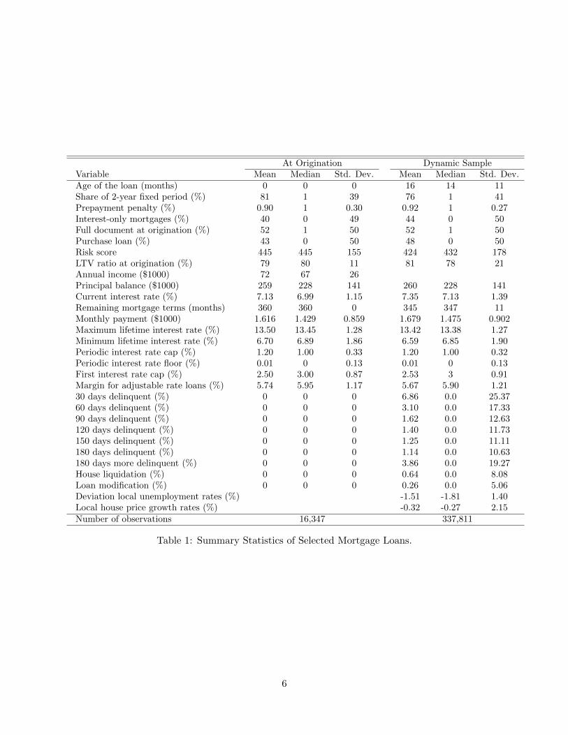
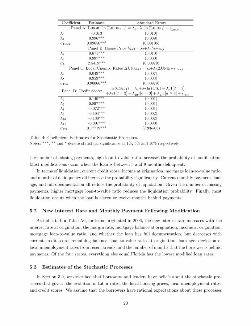
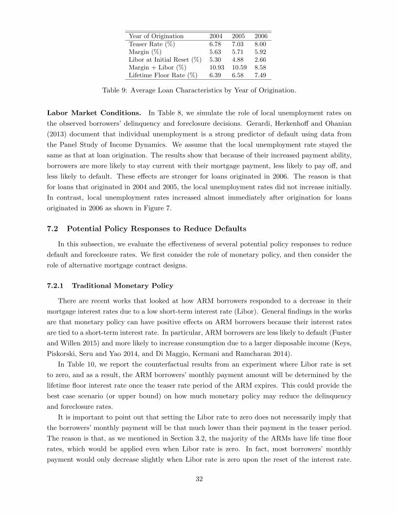
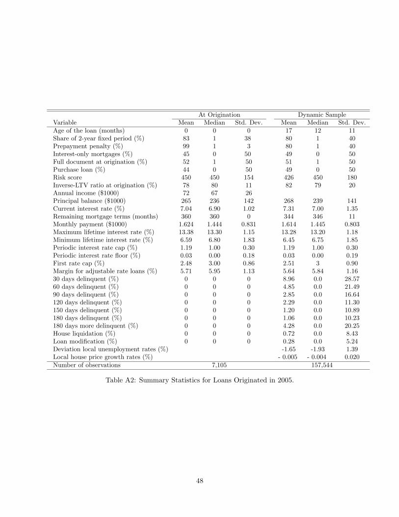
Table 1 provides summary statistics of the mortgage loans at origination and of the whole
dynamic sample period. The average age of the loan is 16 months in the sample and the median is 14
months. At origination, 81 percent of the sample are loans with two-year fixed-rates. Through the
sample period, however, 76 percent of the sample are loans originated with two-year initial fixed-rate
period indicating that more of those loans have terminated via payoff/refinance or foreclosure. Over
90 percent of the loans have prepayment penalty. About 40 percent of the mortgages at origination
are interest-only mortgages and the fraction becomes slightly higher in the whole dynamic sample.
About half of the mortgages have full documentation both at origination and through the sample
period. While 43 percent of the mortgages are purchase loans at the origination, the ratio increases
to 48 percent. Consistent with being subprime, mortgage borrowers in the sample all have relatively
low risk scores, averaging 445 at origination, and the scores deteriorate somewhat as the loans age.8
Additionally, both the average and the median mortgage loan-to-value ratios at origination are both
around 80 percent and they do not change much as the loans age. The annual household income
estimated by TransUnion averages $72,000 at origination with a median of $67,000. Loan balances
average $259,000 at origination with a median of $228,000. These numbers are not very different
from their dynamic counterparts. The mortgage interest rates average 7.13 percent at origination
with a median of 6.99 percent. Dynamically, both the mean and median mortgage interest rates
are higher by 20 and 15 basis points, respectively, as many of these adjustable-rate mortgages reset
7The subprime mortgage market dried up after 2007.8The risk scores are estimated by TransUnion. They range between 150 and 950 with a high score indicating low
Table 1: Summary Statistics of Selected Mortgage Loans.
6
to higher rates after the initial fixed-rate period expires. The ARMs in our data have a lifetime
maximum interest rate of 13.50 percent on average at origination, similar to the dynamic average
of 13.42 percent; and the lifetime minimum interest rate averages 6.7 percent at origination and
6.59 percent in the dynamic sample. The margin above Libor rate when interest rates are adjusted
averages 5.74 percent at origination and 5.67 percent in the dynamic sample. Both at origination
and in the dynamic sample, the period interest rate adjustment has a cap of 1.2 percent and a
floor of 0.01 percent on average. The first interest rate adjustment cap, however, is higher at 2.5
percent on average at origination and 2.53 percent in the dynamic sample. Unemployment rates
tend to be lower than their recent local historical averages. Local house prices, on the other hand,
all depreciate in our sample period.
Two observations emerge from Table 1. First, some mortgages stay in delinquency status for
a long time without being liquidated. Particularly, in our loan-month dynamic sample, close to
7 percent of loans are 30-day delinquent, 3 percent are 60-day delinquent, 2 percent are 90-day
delinquent, etc. Close to 4 percent of the loans are delinquent for over half a year. The liquidation
rate, in contrast, is only 0.64 percent if measured at loan-month level.9 Of course, at the loan level,
2,177 out of the 16,347 loans in our random sample were liquidated (see Table 2), resulting in a
13.3% foreclosure rate, similar to what others have documented in the literature. Second, at the
loan-month level, about 0.26 percent of all mortgage loans are modified by their lenders. This ratio
is obviously much higher if we condition on loans that are delinquent. At the loan level, out of 857
out of the 16,347 loans in our randomly selected sample were modified, resulting in a modification
rate of about 5.24%. We elaborate on the second observation regarding lenders’ decisions in more
details in the next subsection.
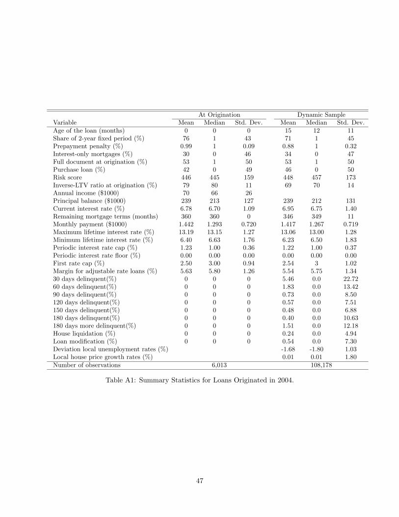
In the appendix, we provide summary statistics of the mortgage loans separately by the origi-
nation year, both at the time of origination and over time in Tables A1 to A3. As can be seen, the
loans originated in later years are riskier, more likely to have two-year interest fixed period instead
of three-year, more likely to be interest-only mortgages, less likely to have full documentation, and
more likely to be purchase loans instead of refinance loans. Their principals, the initial interest rate,
and monthly payment are also larger. Furthermore, the maximum and minimum lifetime interest
rates and margins have risen over time. Given these differences at origination, not surprisingly,
mortgage delinquency rates are much higher for loans originated in later years than earlier years.
2.3 Lenders’ Choices: Descriptive Statistics
From Table 1, we observe that lenders do not always respond to borrowers’ mortgage delinquency
immediately by liquidating them. In this subsection we describe lenders’ decisions in more details.
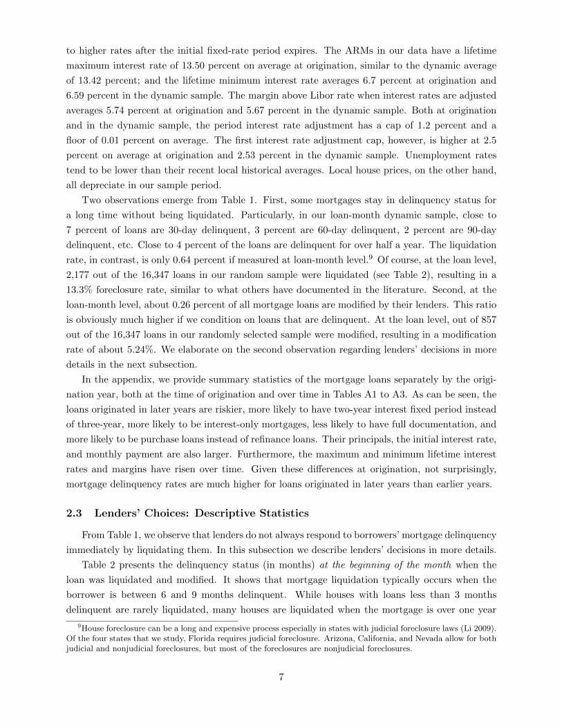
Table 2 presents the delinquency status (in months) at the beginning of the month when the
loan was liquidated and modified. It shows that mortgage liquidation typically occurs when the
borrower is between 6 and 9 months delinquent. While houses with loans less than 3 months
delinquent are rarely liquidated, many houses are liquidated when the mortgage is over one year
9House foreclosure can be a long and expensive process especially in states with judicial foreclosure laws (Li 2009).Of the four states that we study, Florida requires judicial foreclosure. Arizona, California, and Nevada allow for bothjudicial and nonjudicial foreclosures, but most of the foreclosures are nonjudicial foreclosures.
More than 17 months 4.46 2.31Number of observations 2,177 857
Table 2: Loan Status at the Beginning of the Month when Liquidation or Modification Occurs.
delinquent; indeed, about 4.46 percent of the loans liquidated is over 17 months delinquent. As a
side note, the average loan age at liquidation is 27 months; about half of the liquidation occurred
in 2008, 30 percent in 2007, and 8 percent in 2006, and about 6 percent in the first two months of
2009.
Loan modifications are offered generally to loans already in distress. Nearly 60 percent of
the loans are three months or more behind payments at the time of modification. Close to 9
percent are one year or more behind on payments. What is interesting, however, is that about 17
percent of the loans are modified when they are listed as current at the beginning of the period.
The majority of these loans (55 percent) are originated in 2005 and the rest mostly in 2006 (37
percent). Furthermore, the majority of the modifications occur within three months of interest rate
reset.10
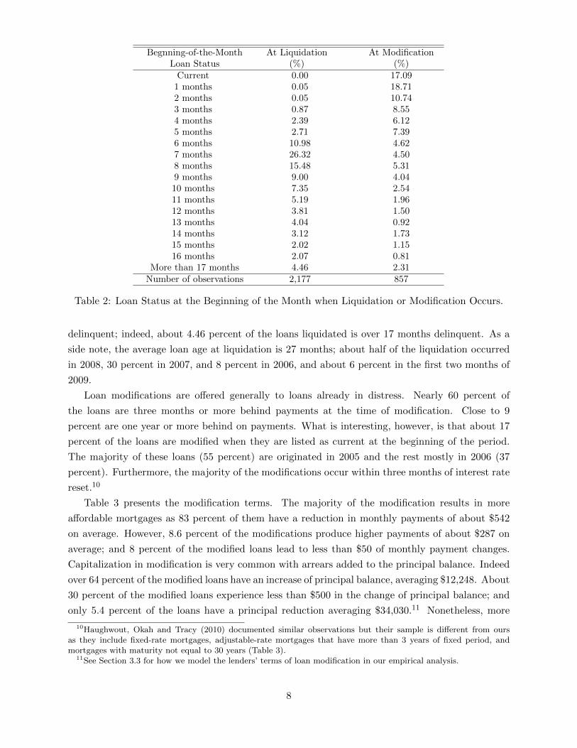
Table 3 presents the modification terms. The majority of the modification results in more
affordable mortgages as 83 percent of them have a reduction in monthly payments of about $542
on average. However, 8.6 percent of the modifications produce higher payments of about $287 on
average; and 8 percent of the modified loans lead to less than $50 of monthly payment changes.
Capitalization in modification is very common with arrears added to the principal balance. Indeed
over 64 percent of the modified loans have an increase of principal balance, averaging $12,248. About
30 percent of the modified loans experience less than $500 in the change of principal balance; and
only 5.4 percent of the loans have a principal reduction averaging $34,030.11 Nonetheless, more
10Haughwout, Okah and Tracy (2010) documented similar observations but their sample is different from oursas they include fixed-rate mortgages, adjustable-rate mortgages that have more than 3 years of fixed period, andmortgages with maturity not equal to 30 years (Table 3).
11See Section 3.3 for how we model the lenders’ terms of loan modification in our empirical analysis.
8
Variable Reduction No Change∗ IncreaseMonthly payment (percentage) 83.41 7.95 8.64Average change in monthly payment ($) -542 1 287
Table 3: Terms of Modification.Notes: No change refers to changes in monthly payment of less than $50 or total loan balancechange of less than $500. Standard deviations are in parenthesis.
than 83 percent of the modified loans have an annualized interest rate reduction averaging 2.98
percent, leading to reduced monthly payment. No modified loans experience interest rate increases.
All of the loans are brought back to being current after modification.
3 The Model
In this section, we present a model of a borrower’s behavior from the time his mortgage is
originated until period T which we specify later. We do not endogenously model lenders’ decisions
in this paper; instead we estimate them parametrically from the data. We assume that borrowers
take lenders’ decisions as given.
Time is discrete, denoted by t = 1, 2, ..., T, with each period representing one month. We use
xt to denote the borrowers’ state vector in period t, which includes time-invariant borrower and
mortgage characteristics (e.g., information collected at mortgage origination, and house location)
as well as time-varying characteristics (e.g., a mortgage’s delinquency status, interest rates, local
housing market condition, local unemployment rates, etc.).
3.1 Choice set
In each period t, after information xt is realized, a borrower chooses an action j. He has three
choices: make the monthly mortgage payment, skip the payment, or pay off the mortgage (which we
denote by “PO”). We assume that the option to pay off the mortgage is available to any borrower,
regardless of their delinquency status.12,13
More specifically, a borrower has different options of making mortgage payments, depending on
the number of late monthly payments he has, which we denote by d where d ≥ 0. If the borrower
12In the data, about 86 percent of those who paid off loans were current in their mortgage at the time of thepayoff, and 9 percent, 2 percent and 1 percent were one-, two-, and three-month delinquent, respectively. Very fewof mortgage payoffs were by borrowers who were more than three months delinquent. Our conversation with theindustry experts suggests that because of information delay, borrowers who have chosen to prepay may sometimes berecorded as one-month delay.
13In reality, a borrower can pay off the mortgage by refinancing or by selling the house. Our data, unfortunately,does not allow us to make such a distinction.
9
is current on his mortgage payment (i.e., d = 0), then he decides whether to make one monthly
payment, which we denote by Pt and specify it below in Equation (2); to miss the payment; or
to pay off the loan.14 If the borrower is one month behind on the payment (i.e., d = 1), then he
can choose to pay just Pt and remain one-month-delinquent; pay 2Pt to bring his status to current
again;15 to miss the payment again and thus his status will be d = 2 next period; or to pay off the
loan. In general, therefore, if a borrower has d ≥ 2 unpaid monthly payments at the beginning of
time t, he can choose to make payments of 0, Pt, 2Pt, · · · , (d + 1)Pt, or paying off the whole loan.
However, we simplify the problem by assuming that, for d ≥ 2, if the borrower decides to pay he
only has the options to pay 0, (d−1)Pt, dPt, or (d+1)Pt to become (d+ 1)-month delinquent, two-
month delinquent, one-month delinquent, or current, respectively, or to pay off the entire loan.16
Formally, a borrower’s choice set with d unpaid payments is denoted by J(d), and given by:
J(d) =
{0, 1,PO}, if d = 0;
{0, 1, 2,PO}, if d = 1;
{0, d− 1, d, d+ 1,PO}, if d ≥ 2,
where the number zero refers to the action of not making any payment, and “PO” refers to paying
off the loan. In the remainder of the paper, we sometimes denote the choice set by J(xt) instead of
J(d) because xt includes the loan delinquency status d. We denote the borrower’s chosen number
of payments in period t as nt ∈ J (dt) .
3.2 State Transition
The evolution of the state variables is captured by the transition probability F (xt+1|xt, j),where, as we discussed previously, xt represents the state vector, and j ∈ J (xt) represents the
borrower’s action at time t. We now discuss each of the state variables.
Interest Rate, Monthly Payment, Mortgage Balance, and Liquidation. A mortgage
contract with adjustable rates specifies the initial interest rate, the length of the period during
which the initial rate is fixed, mortgage maturity, the rate to which the mortgage rate is indexed,
the margin rate, the frequency at which the interest rate is reset, and the cap on interest rate
change in each period, and the mortgage lifetime interest rate cap and floor. As stated in Section
2, we focus on loans that have two or three years fixed interest rate and 30 years maturity. Almost
all of the loans have a six-month adjustment frequency after the initial fixed period.
We now describe how the interest rate evolves through the life of an ARM loan contract. Let
14Given that we model the behavior of a borrower with an adjustable-rate mortgage, a monthly payment is poten-tially time-varying, which is reflected in the time subscript in Pt.
15We do not observe penalty directly in the data. In the model, we allow for different payoff for each decision,which potentially captures the disutility from penalty associated with missing payments, see subsection 3.4 for moredetails.
16In the data, we do not observe borrowers’ payment decisions directly. Instead, we observe their loan status. Inour sample, once a loan becomes d ≥ 2 months delinquent, we do not observe that its delinquency status goes downyet still leave him 3-or-more months delinquent.
10
i0 denote the initial interest rate and let ir denote the new mortgage interest rate at the r-th
reset. For example, i1 denotes the interest rate at the first reset right after the fixed-rate period.
The term Margin represents the margin rate, which is the margin above the index rate that the
new interest will be reset to. All ARMs in our selected sample data are indexed to the six-month
Libor rate, we use Libort to denote the index rate at time t. An ARM contract also specifies a
lifetime interest rate floor and a lifetime interest rate cap, which we denote by LFloor and LCap,
respectively. The ARM interest rate is restricted to be within the band specified by LFloor and
LCap even though Margin above the Libor rate may go outside the band. ARM loan contracts
also specify a cap on the permissible interest rate adjustment in each period, which we denote by
PCap; moreover, for most mortgages, the cap on interest rate change for the first reset at the end
of the initial fixed-rate is different from the subsequent caps, we thus denote the cap on the interest
rate change at the first reset by FCap.17 Combining all the elements, the new interest rate at the
r-th reset in period t(r) evolves as follows:
ir =
max{ir−1 − FCap,LFloor,min
{Margin + Libort(r)−1, ir−1 + FCap,LCap
}}, if r = 1;
max{ir−1 −PCap,LFloor,min
{Margin + Libort(r)−1, ir−1 + PCap,LCap
}}, if r > 1,
(1)
where the first term in Equation (1) is the lowest interest rate the mortgage can have assuming the
periodic interest change takes its maximum allowed value, the second term is the lowest lifetime
interest rate the mortgage can have, and the third term is the lowest of three rates: Libor rate plus
margin, last period interest rate plus the maximum allowed periodic interest adjustment, lifetime
mortgage interest rate cap. Note that Libort(r) evolves stochastically. The borrower, therefore,
needs to form expectations about future values for Libor in order to predict the interest rate he will
have to pay. The values for the other mortgage parameters, {Margin,LFloor,LCap,FCap,PCap}are fixed throughout the life of the mortgage.
It follows from Equation (1) that ir ∈ [max{ir−1 − FCap,LFloor},min{ir−1 + FCap,LCap}]if r = 1 and that ir ∈ [max{ir−1−PCap,LFLoor},min{ir−1+PCap,LCap}] if r > 1. In other
words, {LFloor,LCap,FCap,PCap} put bounds on the volatility of the adjustable mortgage
interest rate: even when Libor is very volatile, the mortgage interest rate may not change signifi-
cantly if FCap, PCap and LCap − LFloor are low.
Given the rule that determines the interest rate reset, we now specify the transition of an ARM
interest rate from period t to period t + 1. With a slight abuse of notation, let r(t) denote the
number of resets that occurred up to period t.18 Note that either r(t+1) = r(t) or r(t+1) = r(t)+1.
The former is true when both period t and t + 1 are in between two resets, hence ir(t+1) = ir(t).
The latter is true when an interest rate is just reset in period t + 1, hence ir(t+1) = ir(t)+1, where
ir(t)+1 is calculated using the formula in (1).
Once the new interest rate is determined, the new monthly payment can be calculated based on
17Typically, FCap is larger than PCap; that is, the interest rate change is typically larger at the initial reset thanat subsequent resets.
18For example, if the initial interest rate is fixed for at least t periods, then r(t) = 0. If an interest rate is reset forthe second time in period t, r(t) = 2.
11
the interest rate and the beginning-of-the-period mortgage balance. Consider a borrower in period t
with remaining mortgage balance Balt−1 and interest rate ir(t). The borrower’s mortgage monthly
payment Pt is calculated so that if the borrower makes a fixed payment of Pt until the 360th period
(i.e., the end of the 30-year loan term), he will pay off the entire mortgage; specifically,
Pt =Balt−1 × ir(t)
/12
1−(1 + ir(t)
/12)−(360−t+1)
, (2)
and the new balance entering period t+ 1 is updated to:
Balt = Balt−1 ×
[1−
ir(t)/
12(1 + ir(t)
/12)360−t+1 − 1
]. (3)
Remark 1. Note that the lenders’ decisions affect the transition of borrowers’ state variables, i.e.,
F (xt+1|xt, j) incorporates the lenders’ responses. If the lender chooses to modify the loan, it will
lead to possible changes to the borrower’s loan status, interest rate, monthly payment and mortgage
balance. We describe how modification affects the mortgage balance, interest rate, monthly payment
and loan status in Section 3.3 below. If the lender chooses to liquidate the house, then the borrower
will be forced to the state of liquidation.
Other State Variables. Other state variables include the number of late monthly payments dt,
the Libor rate Libort, house price ht, changes in local unemployment rate relative to its trend
∆Unrt, borrower credit score CSt, and borrower income Yt. The evolution of these state variables
are as follows:
• Number of late monthly payments (dt): dt+1 = dt − nt + 1, where nt ∈ J (dt) is the number
of monthly payments a borrower makes at time t.
• Libor Rates (Libort): We assume that the borrower’s belief regarding the evolution of Libor
rates is that it follows an AR(1) process in logs
ln(Libort+1) = λ0 + λ1 ln(Libort) + εLibor,t,
where εLibor,t ∼ N(0, σ2Libor) is assumed to be serially independent.
• House price (h): We assume that the borrower’s belief regarding the evolution of housing
prices in each zip code is that it follows an AR(1) process:
ht+1 = λ2 + λ3ht + εh,t,
where εh,t ∼ N(0, σ2h) is assumed to be serially independent.
• Local unemployment rate ( ∆Unrt): We focus on the deviation of the current unemployment
rate Unrt in a county from the average of monthly unemployment rates from 2000 to 2009
12
in the same county Unr, which we denote by ∆Unrt = Unrt − Unr. We assume that the
borrower’s belief regarding the evolution of ∆Unr is that it follows an AR(1) process:
∆Unrt+1 = λ4 + λ5∆Unrt + εUnr,t,
where εUnr,t ∼ N(0, σ2∆Unr) is assumed to be serially independent.
• Credit score (CSt): We assume that the borrower’s belief regarding the evolution of the log
of his credit score is that it has the following process:
where 1 (·) is the indicator function and εCS,t ∼ N(0, σ2CS) is assumed to be serially indepen-
dent.
3.3 Loan Modification and Foreclosure
A lender makes the following decisions each period: foreclose the house, modify the loan, or wait
(i.e., do nothing). As we mentioned in the introduction, in this paper we do not endogenize these
decisions; rather, we assume that lenders follow decision rules that depend on borrowers’ various
characteristics and are invariant to policy changes.19 Borrowers take these decision rules as given.
As we describe in detail in Section 5.1, we specify that the probability that the lenders will
choose one of the three options depends on the delinquency status, and a rich set of loan and
housing characteristics. We estimate these lender decision rules by flexible logit or multinomial
logit regressions.
If the lender chooses to foreclose a house, the borrower receives the payoff associated with
liquidation (see Eq. (6) below). If the lender chooses to wait, then the borrowers’ terms of the loan
stay unchanged. However, if the lender chooses to modify a loan, we need to specify the new terms
of the modified loan. Here we recall from Table 3 in Section 2 that the most popular modification
is recapitalization coupled with interest rate reset. Ideally we would like to estimate lenders’ bi-
dimensional choice of the new balance and new interest rate of the modified loan; however, instead
of estimating such a joint process, we assume for simplicity that the new term of the modified loan
is determined as follows:
• After modification, borrowers’ payment status is brought to current, i.e., dt+1 = 0;
• The new balance upon modification will be the sum of the pre-modification loan balance and
19This characterization of lender behavior is consistent with the data. In a companion paper, we endogenize lenders’decisions and investigate why they did not respond to the various policies introduced by the government to reduceforeclosures and encourage loan modifications.
13
the arrears in late payments, i.e.,20
Balt+1 = Balt + dt · Pt, if the loan is modified at time t.
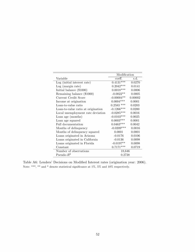
• The modified loan is a fixed rate mortgage with the maturity equal to the remainder of the
initial loan, and the new modified interest rate, and thus the new monthly payment upon
loan modification, is specified as a function of the initial monthly payment, initial interest
rate, initial loan balance, margin rate, and states of the property. We estimate this process
for the modified monthly payment directly from the data and by the year of the mortgage
origination.
3.4 Payoff Function
We specify a borrower’s current-period payoff from taking action j in period t as
uj(xt) + εjt,
where uj(xt) is a deterministic function of xt and εjt is a choice-specific preference shock. The
vector εt ≡(ε1t, · · · εJ(xt)t
)is drawn from Type-I Extreme Value distribution and we assume that
εt is independently and identically distributed over time.
When a borrower with d late payments makes n monthly payments, but does not pay off the
mortgage, we assume that the deterministic part of his period-t payoff is:
The first term β1Pt represents the disutility from one month’s payment. The second term β2(n−1)Pt
is the disutility of n− 1 months’ payment.21 The term β3CSt determines the borrower’s ability (or
willingness) to make a payment. Specifically, CSt is the borrower’s updated current credit score
provided by TransUnion, and it captures not only the borrower’s past payment history but also
his ability to obtain future credit. We also allow credit scores to interact with borrowers’ payment
decisions, Pt and (n − 1)Pt, and the parameters β4 and β5 capture those interaction effects. The
term Y0 represents the borrower’s income at origination; and ∆Unrt captures the deviations of
the current local market condition relative to its long-run average. The term X0 is a collection of
the borrower’s characteristics at origination which contains original monthly payment amount (P0),
inverse loan-to-value ratio at origination (ILTV0), the year of loan origination, and whether the
borrower’s income is fully documented. ξd is a dummy variable for the borrower’s payment status
20As shown in Table 3, a small fraction of modified loans (about 5 percent) received a balance reduction in oursample. We assume that these borrowers are “surprised” by the unexpected changes in their loan balance. In ourfuture research where we endogenize the lenders’ choices, we will endogenously determine the lenders’ choices of newmortgage and interest rate upon modification.
21We use β1Pt + β2(n − 1)Pt, instead of a single term β1nPt to allow for the possibility that paying more than asingle monthly payment amount could have a different utility cost than making only one payment.
14
d at the beginning of the period. In order to reduce the number parameters to be estimated, we
assume that for d ≥ 4,
ξd = ξ4,0 + dξ4,1
Finally, ζn is a constant for taking action n. We also make the assumption that for n ≥ 4,
ζn = ζ4,0 + nζ4,1.
We normalize ζ0 = 0 because only relative utility is identified in a discrete choice model.
When a borrower chooses to pay off the mortgage (j = PO), the deterministic part of the flow
Where δ is the discount factor (which we set to be 0.99 in our estimation), PPNt is an indicator
for whether the borrower has to pay a prepayment penalty if prepaying in period t, ILTVt is the
ratio of the borrower’s current house price to the remaining balance, i.e., the inverse of mortgage
loan-to-value ratio, and ILTV0 is the inverse mortgage loan-to-value ratio at origination.22 We
assume that the model is terminated when the borrower pays off the mortgage.23 ζPO,d determines
the utility from paying off depending on the borrower’s payment status d at the beginning of the
period. As before, in order to reduce the number parameters to be estimated, we assume that for
d ≥ 3,
ζPO,d = ζPO,3,0 + dζPO,3,1.
If the house is liquidated, then as we mentioned earlier the borrower’s continuation value is give
by:
Vt(liquidated) = ζ liquid,state. (6)
Note that we allow ζ liquid,state to depend on state of the property in order to capture state level dif-
ferences that are not captured by the model such as legislative differences regarding the foreclosure
process. We normalize ζ liquid,NV to zero.
If the borrower does not pay off the mortgage by period T , and if the borrower’s house is not
liquidated by period T , the borrower reaches the final period T .24 The model is then terminated,
22We assume that the house price follows an AR(1) process with the shock drawn from a normal distribution. Theinverse of a normal random variable, however, does not have mean. In the analysis, we therefore use the inverseloan-to-value ratio ILTV instead of the mortgage loan-to-value ratio.
23We make this assumption because the mortgage loan exits our database once the borrower pays off or refinancethe mortgage.
24To simplify the problem, we do not follow mortgages to their actual terminal period, that is, 360 months. Asshown in the data section, most borrowers either pay off their mortgages or become seriously delinquent within thefirst six years after mortgage origination.
15
and the borrower receives the terminal payoff:
VT (xT ) =
β15 + β16CST + β17ILTVT , if current at T
0, otherwise.(7)
Remark 2. In our framework, we assume that the lender can directly affect a borrower’s current-
period flow utility only if the lender forecloses (i.e., liquidates) the house. If the lender chooses
to modify the loan terms, or wait, the borrower’s flow utility is affected only to the extent that
the modified loan term affects the borrower’s monthly payment. Dynamically the lender’s choices
obviously affect the borrower’s ability to stay current in the mortgage and subsequently the probability
of being foreclosed.
3.5 Value Function
The borrower sequentially maximizes the sum of expected discounted flow payoffs in each period
t = 1, ..., T . Let σt (xt, εt) be the borrower’s choice at time t given the state vector xt and the vector
of choice-specific shocks εt, such that σt,j(xt, εt) = 1 if a borrower chooses action j given (xt, εt); and
0 otherwise. Let σ ≡ (σ1, ..., σT ) denote the borrower’s decision profile from period 1 to T where
σT , the terminal-period decision rule is included for ease of exposition, but the borrower makes no
choices (see the discussion prior to Eq. (7)). We can then express the borrower’s value functions
from decision profile σ ≡ (σ1, ..., σT ) recursively as follows: for t ≤ T − 1,
Vt(xt;σ) = Eεt
∑j∈J(xt)
σt,j(xt, εt)
{uj(xt) + εjt + δ
∫xt+1∈Xt
Vt+1(xt+1;σ)dF (xt+1|xt, j)
} , (8)
and VT (xT ;σ) is given by (7). The borrower’s optimal decision rule σ∗ is such that Vt(xt;σ∗) ≥
Vt(xt;σ) for any possible decision rule σ, and for all xt, where t = 1, · · · , T .
4 Estimation
We define the choice-specific value function for action j in period t ≤ T − 1, vt,j(xt), under
decision profile σ∗, as
vt,j(xt) = uj(xt) + δ
∫xt+1∈Xt
Vt+1(xt+1;σ∗)dF (xt+1|xt, j). (9)
The value function Vt (xt;σ∗) can then be written as:
Vt(xt;σ∗) = Eεt
∑j∈J(xt)
σ∗t,j(xt, εt) {vt,j(xt) + εjt}
. (10)
In order to solve for the optimal decision profile σ∗, we use backward induction following the
standard methods in dynamic discrete choice models with a finite number of periods (see, for
16
example, Rust 1987, 1994a, and 1994b, and Keane and Wolpin 1993). We start from the penultimate
period T − 1. The choice-specific value function in period T − 1 is given by:
vT−1,j(xT−1) = uj(xT−1) + δ
∫xT∈XT
VT (xT ;σ∗)dF (xT |xT−1, j),
where VT (xT ;σ∗) is given by (7), and σ∗T is null. The optimal decision rule in period T − 1 is then:
Given the functional-form assumption for εT−1, we can show, following Rust (1987), that
VT−1(xT−1;σ∗) = ln
∑j′∈J(xT−1)
exp(vT−1,j′(xT−1))
+ γ, (12)
where γ is the Euler constant.
Now let us consider the borrower’s optimal decision rule in period T − 2. In order to cal-
culate vT−2,j(xT−2), we need to know∫xT−1∈XT−1
VT−1(xT−1;σ∗)dF (xT−1|xT−2, j), which can be
calculated using equation (12) and the state transition function F (xT−1|xT−2, j) . We then derive
σ∗T−2,j(xT−2, εT−2) and VT−2(xT−2;σ∗) analogous to what we did in period T − 1. We repeat this
process until we reach the initial period. The borrower’s optimal decision rule in period t is:
σ∗t,j(xt, εt) = 1 if vt,j(xt) + εjt ≥ maxj′∈J(xt)
{vt,j′(xt) + εj′t
}, (13)
and the period-t continuation value function is:
Vt(xt;σ∗) = ln
∑j′∈J(xt)
exp(vt,j′(xt)
)+ γ. (14)
Moreover, a borrower’s conditional choice probability under the optimal decision profile σ∗ for
alternative j ∈ J (xt) in period t when the state vector is xt is given by:
pt,j(xt;σ∗) = Eεt [σ
∗t,j(xt, εt)] =
exp(vt,j(xt))∑j′∈J(xt)
exp(vt,j′(xt)). (15)
We estimate the model using maximum likelihood. In the data, we observe a path of states and
choices for each individual i: (xi, ai) ≡ {(xit, ait)}Tt=1, where ait ≡ {aijt}j∈J(xit), and aijt is defined to
be a dummy variable that equals one when individual i chooses action j in period t. The likelihood
of observing (xi, ai) given initial state xi1 and parameter vector θ for individual i is:
L(xi, ai|xi1; θ) =T−1∏t=1
lt(ait, x
it+1|xit; θ), (16)
where∏T−1t=1 l(ait, x
it+1|xit; θ) is the likelihood of observing action ait in period t and observing the
17
state to transition to xit+1 in period t + 1 given state xit and parameter vector θ, as predicted by
the model, and it is given by:
lt(ait, x
it+1|xit; θ) =
∏j∈J(xit)
[pt,j(x
it;σ∗ (θ))f(xit+1|xit, j)
]aijt . (17)
where pt,j (·; ·) is given by (15) and σ∗ (θ) is the model’s predicted optimal decision profile for the
borrower given parameter vector θ. Parameter estimate θ∗ maximizes the log-likelihood for the
whole sample, i.e,
θ∗ = arg max lnL(θ) =I∑i=1
ln(L(xi, ai|xi1; θ)
)= arg max
I∑i=1
T−1∑t=1
∑j∈J(xit)
aijt[ln(pt,j(x
it;σ∗ (θ))
)+ ln f(xit+1|xit, j)
]. (18)
5 Estimation Results
5.1 Lenders’ Decisions
As previously discussed, we estimate lenders’ policy functions parametrically using logit or
multinomial logit regressions. The borrower enters period t with a delinquent status dt, makes
the payment decision at, after which the lender makes the decisions regarding whether to modify,
liquidate, or do nothing about the loan based on the delinquent status of the loan at the end of the
period t.25 However, in the data we only observe the loan status at the beginning of the period.
Thus when we observe that a loan was current in period t and was also modified in period t, we
assume that the loan would have been one month late at the end of period t had the modification
not taken place.
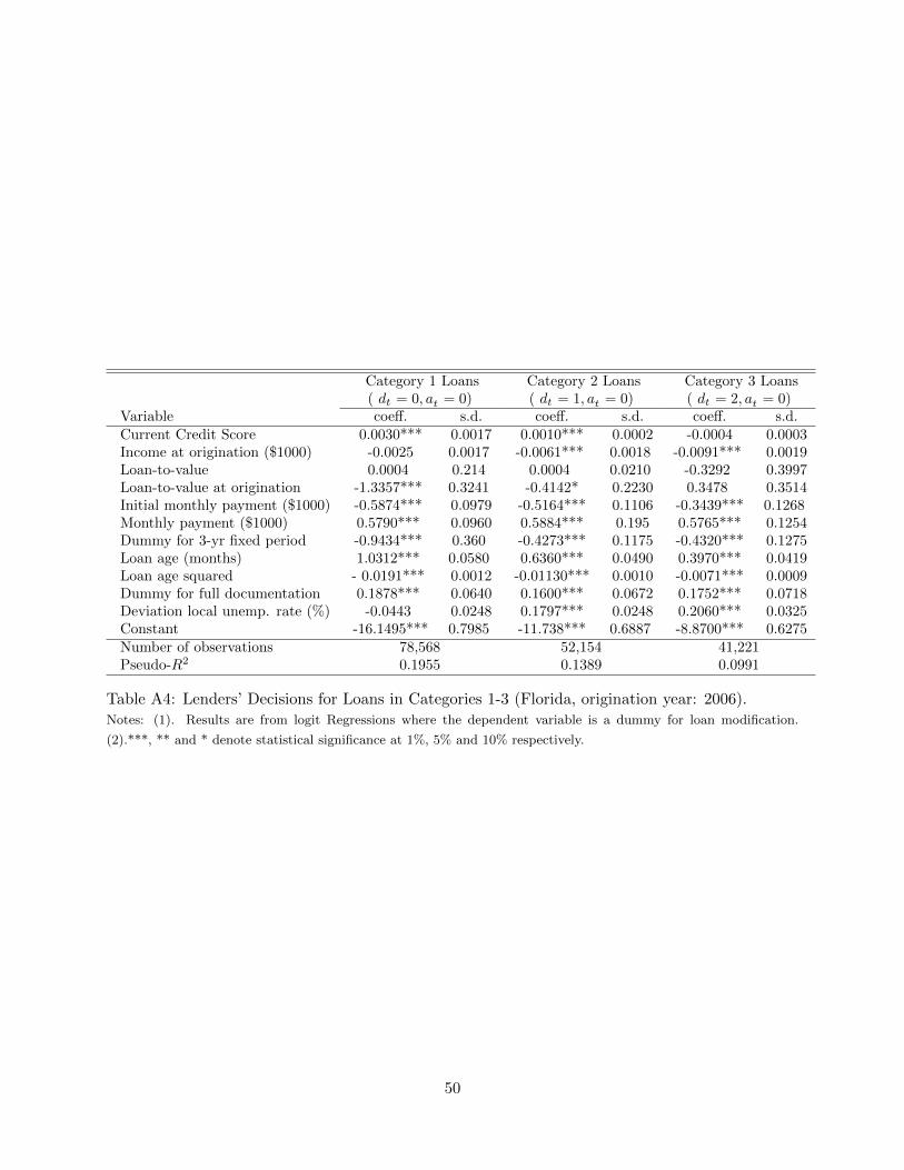
Specifically, we estimate the lenders’ decisions separately for four categories of loans:
Category 1: (dt = 0, at = 0) . Borrowers are current in the beginning of the period, but do not
make a payment in the period;
Category 2: (dt = 1, at = 0) . Borrowers are one month delinquent in the beginning of the period,
but do not make a payment in the period;
Category 3: (dt = 2, at = 0) . Borrowers are two month delinquent in the beginning of the period,
but do not make a payment in the period;
Category 4: (dt ≥ 3, at = 0) . Borrowers are three-or-more-month delinquent at the beginning of
a period, but do not make a payment in the period.
It is important to note that lenders only modify or liquidate a loan if the borrower does not
make any payment in the period. Therefore, if a borrower who enters the period with loan status
25We do not separately model lenders’ decision when to start foreclosure. As long as foreclosure is not complete,we consider the lender as “waiting.”
18
dt ≥ 1, and if he makes at ≥ 1 payment, the lender’s only choice is waiting even though the status
of the loan at the end of the period may still be one or more month delinquent if at < dt + 1.
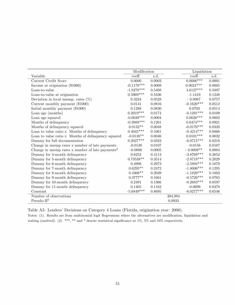
In our specification of the lenders’ decisions, we recall from Table 2 that lenders almost never
liquidate a house whose mortgage is less than three months delinquent. Thus we assume that
for loans in categories 1 to 3, the lenders choose only between modification and waiting ; and
the probability of modification is specified as a logit function of the state variables that includes
borrower characteristics and loan status.26 For loans in category 4, we assume that lenders decides
among three options: modification, liquidation, and waiting. We specify a multinomial logit function
to represent the lenders’ probabilities of choosing the three alternatives. We further condition
lenders’ decisions on state and year of origination. Finally, we also estimate lenders’ decision
on interest rates for modified loans. Given the much smaller number of modified loans, we only
condition this decision on mortgage year of origination. In total, we have 51 regressions (4 states x 3
origination years x 4 loan status + 3 origination years for interest rate estimation). To save space,
we only report the estimation results for lenders’ modification, foreclosure, or wait decisions for
loans originated in 2006 in Florida in Appendix Tables A4 and A5. Estimation results for interest
rates after modification for loans originated in year 2004 are reported in Table A6.27
Category 1 Loans. For category 1 loans originated in Florida in 2006, lenders are more likely
to modify if the borrower has a high credit score, high monthly payment but low initial monthly
payment, and full documentation. An older loan is also more likely to be modified. By contrast,
mortgage loans with high initial mortgage loan-to-value ratios and three-year fixed interest periods
are less likely to be modified.
Category 2 Loans. For category 2 loans originated in Florida in 2006, the factors that explain
modification probability are similar to those that are current at the beginning of the period with a
few exceptions. Income at origination reduces the probability of being modified while increases in
local unemployment rates relative to recent trends raise the modification probability.
Category 3 Loans. For category 3 loans originated in Florida in 2006, similar factors determine
the likelihood of being modified by lenders as those for Category 2 loans. The only exception is that
loan-to-value ratio at origination and credit scores no longer matter for modification probability.
Category 4 Loans. For category 4 loans, we include many more explanatory variables to our
multinomial logit regressions. A loan is more likely modified if income at origination is low, loan-to-
value ratio is low, initial loan-to-value ratio is high, the loan is older, or it has full documentation.
A loan, however, is less likely to be modified if the borrower has many missed payments. Given
26In our estimation, we dropped the few (specifically, 4 case) loans of category 1 to 3 that were liquidated. Thatis, we assume that the four borrowers were making choices assuming that foreclosure would not have happened yet.We did not include their terminal liquidation in the likelihood function to avoid degeneracy.
27To increase the precision, we use the full sample, instead of the 1.75 percent random sample, in estimating lenders’decisions.
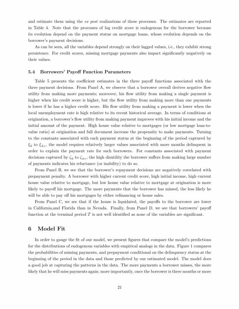
Panel C: Coefficients in Vt(liquidated) as specified in (6)ζliquid,AZ 0.3358 0.2363ζliquid,CA -1.0123*** 0.2008ζliquid,FL -3.5621*** 0.2688
Panel D: Coefficients in VT (xT ) as specified in (7)Constant (β15) -3.3825 (65.9577)CSt (β16) -0.0847 (4.0928)ILTVT (β17) -0.5666 (43.7830)
Table 5: Coefficient Estimates for Borrowers’ Payoff Functions.Notes: ***, ** and * denote statistical significance at 1%, 5% and 10% respectively.
22
0.2
.4.6
.81
0 5 10Number of Late Monthly Payments
Data Model
Probability of Missing Payments
0.0
1.0
2.0
3.0
4
0 5 10Number of Late Monthly Payments
Data Model
Probability of Prepayment
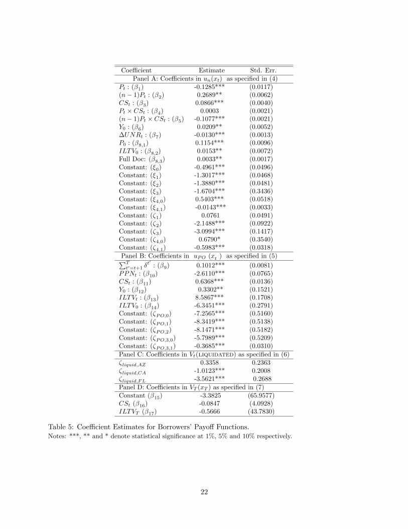
Figure 1: Probabilities of Missing Payments and Prepayment, By Beginning-of-Period DelinquencyStatus.
behind his payment schedule, he will stay delinquent with almost certainty. The model also captures
the relationship between months of delinquency and the probability of prepayment; interestingly,
the model predicts that the probability of prepayment is highest among those borrowers who are
one month late in their payment.
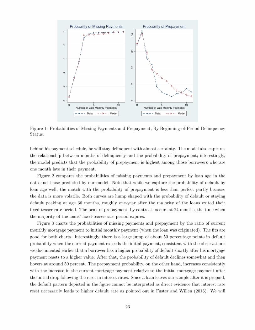
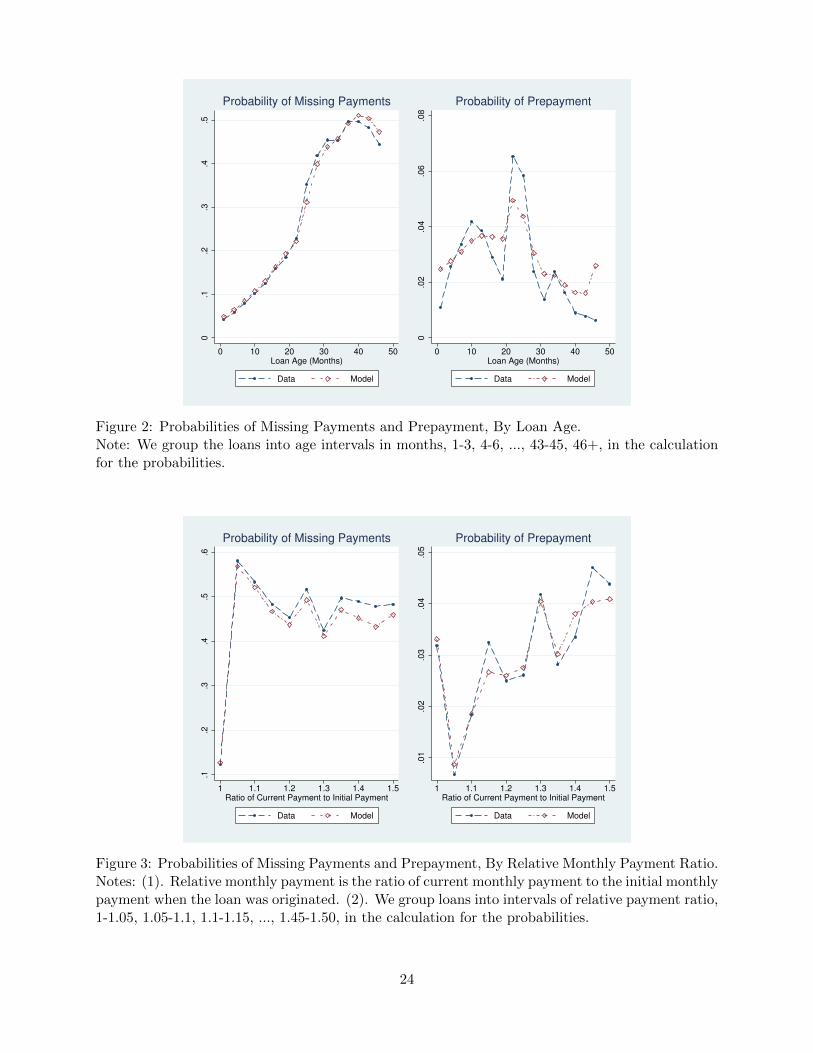
Figure 2 compares the probabilities of missing payments and prepayment by loan age in the
data and those predicted by our model. Note that while we capture the probability of default by
loan age well, the match with the probability of prepayment is less than perfect partly because
the data is more volatile. Both curves are hump shaped with the probability of default or staying
default peaking at age 36 months, roughly one-year after the majority of the loans exited their
fixed-teaser-rate period. The peak of prepayment, by contrast, occurs at 24 months, the time when
the majority of the loans’ fixed-teaser-rate period expires.
Figure 3 charts the probabilities of missing payments and prepayment by the ratio of current
monthly mortgage payment to initial monthly payment (when the loan was originated). The fits are
good for both charts. Interestingly, there is a large jump of about 50 percentage points in default
probability when the current payment exceeds the initial payment, consistent with the observations
we documented earlier that a borrower has a higher probability of default shortly after his mortgage
payment resets to a higher value. After that, the probability of default declines somewhat and then
hovers at around 50 percent. The prepayment probability, on the other hand, increases consistently
with the increase in the current mortgage payment relative to the initial mortgage payment after
the initial drop following the reset in interest rates. Since a loan leaves our sample after it is prepaid,
the default pattern depicted in the figure cannot be interpreted as direct evidence that interest rate
reset necessarily leads to higher default rate as pointed out in Fuster and Willen (2015). We will
23
0.1
.2.3
.4.5
0 10 20 30 40 50Loan Age (Months)
Data Model
Probability of Missing Payments
0.0
2.0
4.0
6.0
8
0 10 20 30 40 50Loan Age (Months)
Data Model
Probability of Prepayment
Figure 2: Probabilities of Missing Payments and Prepayment, By Loan Age.Note: We group the loans into age intervals in months, 1-3, 4-6, ..., 43-45, 46+, in the calculationfor the probabilities.
.1.2
.3.4
.5.6
1 1.1 1.2 1.3 1.4 1.5Ratio of Current Payment to Initial Payment
Data Model
Probability of Missing Payments
.01
.02
.03
.04
.05
1 1.1 1.2 1.3 1.4 1.5Ratio of Current Payment to Initial Payment
Data Model
Probability of Prepayment
Figure 3: Probabilities of Missing Payments and Prepayment, By Relative Monthly Payment Ratio.Notes: (1). Relative monthly payment is the ratio of current monthly payment to the initial monthlypayment when the loan was originated. (2). We group loans into intervals of relative payment ratio,1-1.05, 1.05-1.1, 1.1-1.15, ..., 1.45-1.50, in the calculation for the probabilities.
24
.1.2
.3.4
.5.6
40 60 80 100 120Loan to Value Ratio
Data Model
Probability of Missing Payments
0.0
2.0
4.0
6.0
8
40 60 80 100 120Loan to Value Ratio
Data Model
Probability of Prepayment
Figure 4: Probabilities of Missing Payments and Prepayment, By the Current Mortgage Loan-to-Value (LTV) Ratio.Notes: (1). Unit for LTV is in percentage. (2). We group loans into intervals of LTVs, 50-, [50,60), [60,70), ..., [110,120), 120+, in the calculation for the probabilities.
address this issue in details in the next section.
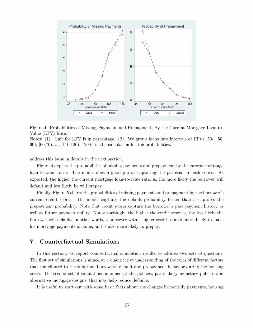
Figure 4 depicts the probabilities of missing payments and prepayment by the current mortgage
loan-to-value ratio. The model does a good job at capturing the patterns in both series. As
expected, the higher the current mortgage loan-to-value ratio is, the more likely the borrower will
default and less likely he will prepay.
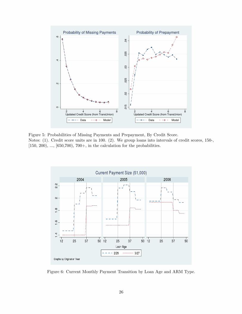
Finally, Figure 5 charts the probabilities of missing payments and prepayment by the borrower’s
current credit scores. The model captures the default probability better than it captures the
prepayment probability. Note that credit scores capture the borrower’s past payment history as
well as future payment ability. Not surprisingly, the higher the credit score is, the less likely the
borrower will default. In other words, a borrower with a higher credit score is more likely to make
his mortgage payments on time, and is also more likely to prepay.
7 Counterfactual Simulations
In this section, we report counterfactual simulation results to address two sets of questions.
The first set of simulations is aimed at a quantitative understanding of the roles of different factors
that contributed to the subprime borrowers’ default and prepayment behavior during the housing
crisis. The second set of simulations is aimed at the policies, particularly monetary policies and
alternative mortgage designs, that may help reduce defaults.
It is useful to start out with some basic facts about the changes in monthly payments, housing
25
0.2
.4.6
2 4 6 8Updated Credit Score (from TransUnion)
Data Model
Probability of Missing Payments
.015
.02
.025
.03
.035
.04
2 4 6 8Updated Credit Score (from TransUnion)
Data Model
Probability of Prepayment
Figure 5: Probabilities of Missing Payments and Prepayment, By Credit Score.Notes: (1). Credit score units are in 100. (2). We group loans into intervals of credit scores, 150-,[150, 200), ..., [650,700), 700+, in the calculation for the probabilities.
Figure 6: Current Monthly Payment Transition by Loan Age and ARM Type.
26
Figure 7: Housing Price and Unemployment Rate Trends, by Year of Origination of Loans.
prices and unemployment rates that the ARM borrowers in our dataset face as their loans age. In
Figure 6, we show the average monthly payment amounts as loans age, for 2/28 (2 years fixed rate,
28 years adjustable rate) and 3/27 (3 years fixed rate, 27 years adjustable rate) ARM mortgages.
It shows that upon the end of the initial lower teaser rate period, borrowers’ monthly payment
would typically increase substantially for loans that originated in 2004 and 2005, in contrast, it will
decrease substantially for loans that originated in 2006. These observations are not surprising as
interest rates moved down substantially after 2007.
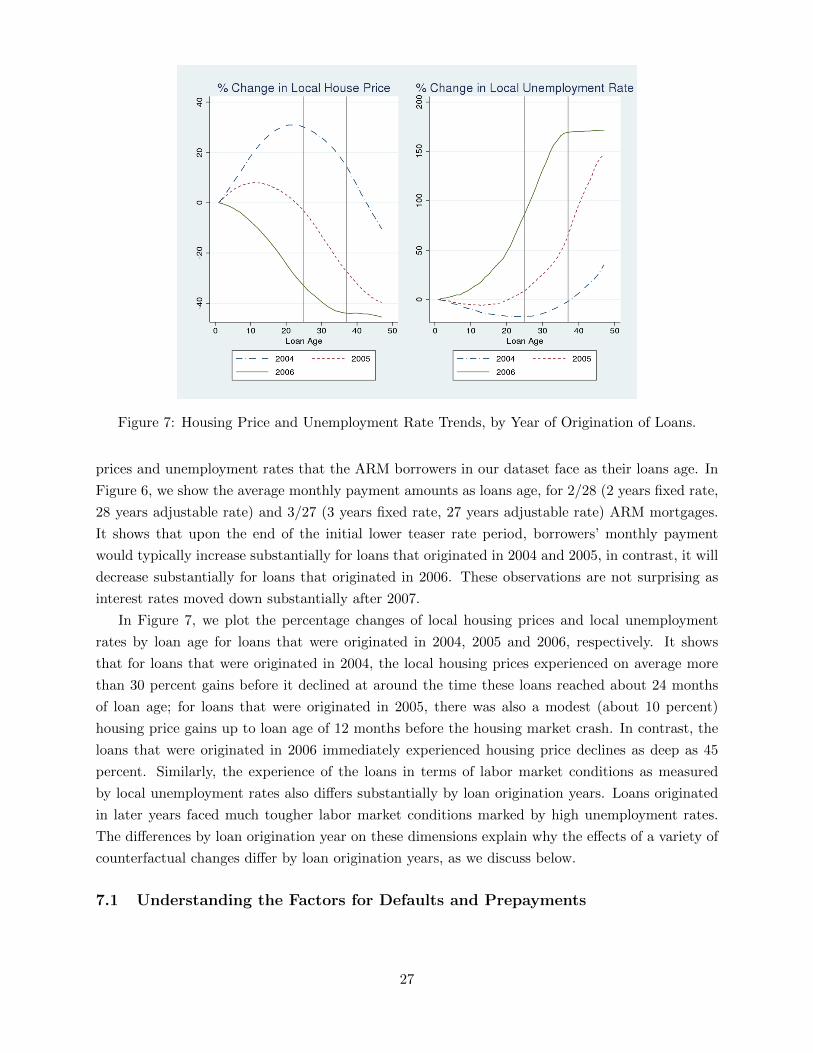
In Figure 7, we plot the percentage changes of local housing prices and local unemployment
rates by loan age for loans that were originated in 2004, 2005 and 2006, respectively. It shows
that for loans that were originated in 2004, the local housing prices experienced on average more
than 30 percent gains before it declined at around the time these loans reached about 24 months
of loan age; for loans that were originated in 2005, there was also a modest (about 10 percent)
housing price gains up to loan age of 12 months before the housing market crash. In contrast, the
loans that were originated in 2006 immediately experienced housing price declines as deep as 45
percent. Similarly, the experience of the loans in terms of labor market conditions as measured
by local unemployment rates also differs substantially by loan origination years. Loans originated
in later years faced much tougher labor market conditions marked by high unemployment rates.
The differences by loan origination year on these dimensions explain why the effects of a variety of
counterfactual changes differ by loan origination years, as we discuss below.
7.1 Understanding the Factors for Defaults and Prepayments
27
Loan Baseline Fixed Rate MortgageAge Current Paid off Delinquent [Liquidated] Current Paid off Delinquent [Liquidated]
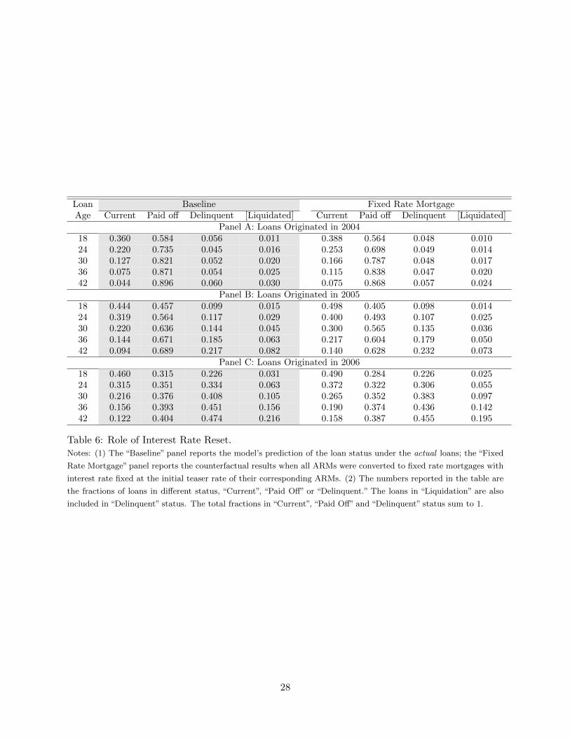
Table 6: Role of Interest Rate Reset.Notes: (1) The “Baseline” panel reports the model’s prediction of the loan status under the actual loans; the “Fixed
Rate Mortgage” panel reports the counterfactual results when all ARMs were converted to fixed rate mortgages with
interest rate fixed at the initial teaser rate of their corresponding ARMs. (2) The numbers reported in the table are
the fractions of loans in different status, “Current”, “Paid Off” or “Delinquent.” The loans in “Liquidation” are also
included in “Delinquent” status. The total fractions in “Current”, “Paid Off” and “Delinquent” status sum to 1.
28
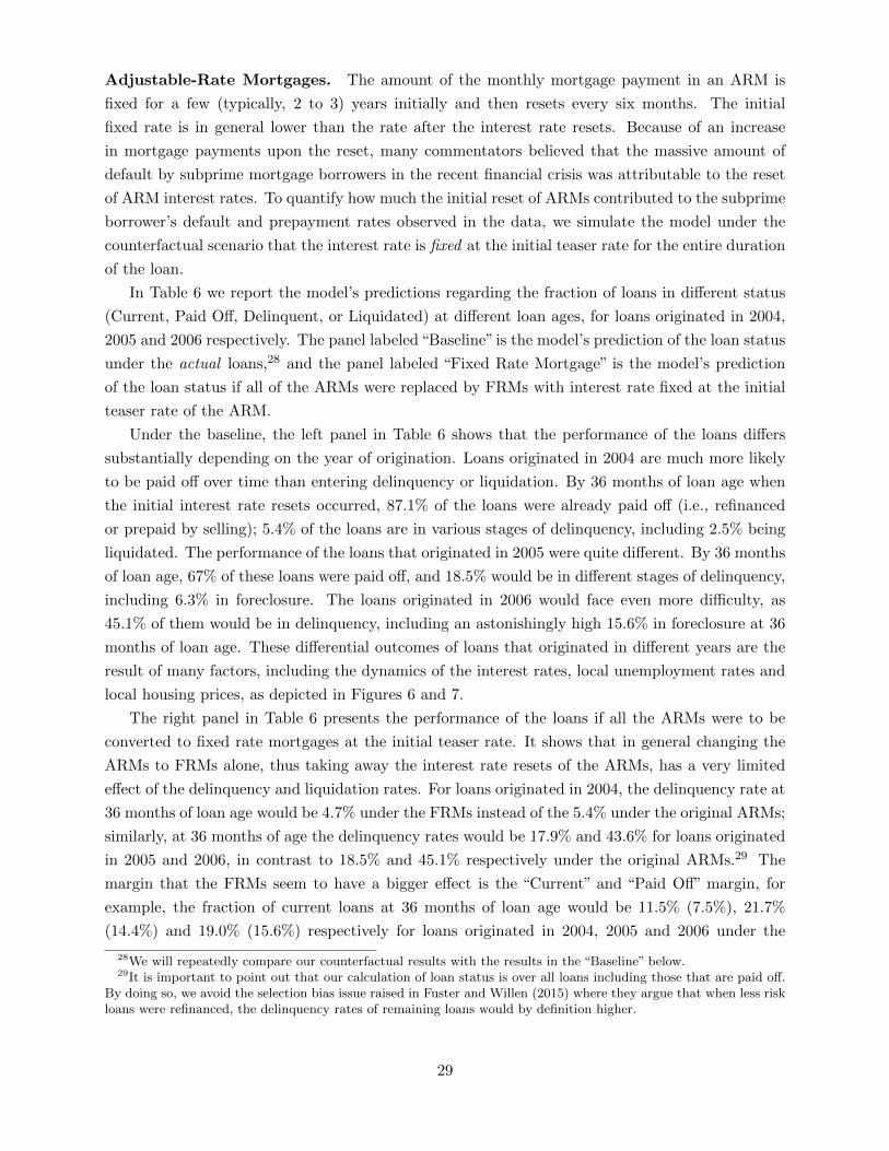
Adjustable-Rate Mortgages. The amount of the monthly mortgage payment in an ARM is
fixed for a few (typically, 2 to 3) years initially and then resets every six months. The initial
fixed rate is in general lower than the rate after the interest rate resets. Because of an increase
in mortgage payments upon the reset, many commentators believed that the massive amount of
default by subprime mortgage borrowers in the recent financial crisis was attributable to the reset
of ARM interest rates. To quantify how much the initial reset of ARMs contributed to the subprime
borrower’s default and prepayment rates observed in the data, we simulate the model under the
counterfactual scenario that the interest rate is fixed at the initial teaser rate for the entire duration
of the loan.
In Table 6 we report the model’s predictions regarding the fraction of loans in different status
(Current, Paid Off, Delinquent, or Liquidated) at different loan ages, for loans originated in 2004,
2005 and 2006 respectively. The panel labeled“Baseline” is the model’s prediction of the loan status
under the actual loans,28 and the panel labeled “Fixed Rate Mortgage” is the model’s prediction
of the loan status if all of the ARMs were replaced by FRMs with interest rate fixed at the initial
teaser rate of the ARM.
Under the baseline, the left panel in Table 6 shows that the performance of the loans differs
substantially depending on the year of origination. Loans originated in 2004 are much more likely
to be paid off over time than entering delinquency or liquidation. By 36 months of loan age when
the initial interest rate resets occurred, 87.1% of the loans were already paid off (i.e., refinanced
or prepaid by selling); 5.4% of the loans are in various stages of delinquency, including 2.5% being
liquidated. The performance of the loans that originated in 2005 were quite different. By 36 months
of loan age, 67% of these loans were paid off, and 18.5% would be in different stages of delinquency,
including 6.3% in foreclosure. The loans originated in 2006 would face even more difficulty, as
45.1% of them would be in delinquency, including an astonishingly high 15.6% in foreclosure at 36
months of loan age. These differential outcomes of loans that originated in different years are the
result of many factors, including the dynamics of the interest rates, local unemployment rates and
local housing prices, as depicted in Figures 6 and 7.
The right panel in Table 6 presents the performance of the loans if all the ARMs were to be
converted to fixed rate mortgages at the initial teaser rate. It shows that in general changing the
ARMs to FRMs alone, thus taking away the interest rate resets of the ARMs, has a very limited
effect of the delinquency and liquidation rates. For loans originated in 2004, the delinquency rate at
36 months of loan age would be 4.7% under the FRMs instead of the 5.4% under the original ARMs;
similarly, at 36 months of age the delinquency rates would be 17.9% and 43.6% for loans originated
in 2005 and 2006, in contrast to 18.5% and 45.1% respectively under the original ARMs.29 The
margin that the FRMs seem to have a bigger effect is the “Current” and “Paid Off” margin, for
example, the fraction of current loans at 36 months of loan age would be 11.5% (7.5%), 21.7%
(14.4%) and 19.0% (15.6%) respectively for loans originated in 2004, 2005 and 2006 under the
28We will repeatedly compare our counterfactual results with the results in the “Baseline” below.29It is important to point out that our calculation of loan status is over all loans including those that are paid off.
By doing so, we avoid the selection bias issue raised in Fuster and Willen (2015) where they argue that when less riskloans were refinanced, the delinquency rates of remaining loans would by definition higher.
29
FRMs (respectively, under the original ARMs).
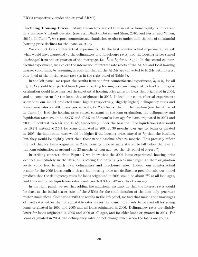
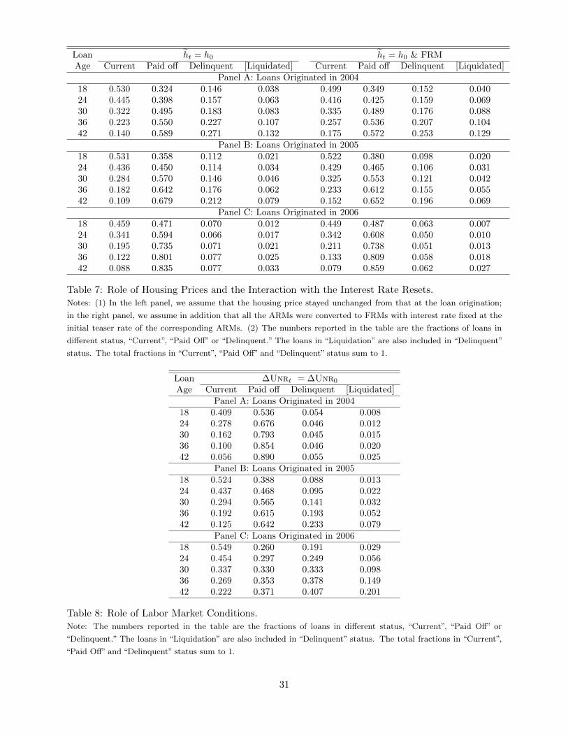
Declining Housing Prices. Many researchers argued that negative home equity is important
in a borrower’s default decision (see, e.g., Bhutta, Dokko, and Shan, 2010; and Fuster and Willen,
2015). In Table 7, we report counterfactual simulation results to understand the role of substantial
housing price declines for the loans we study.
We conduct two counterfactual experiments. In the first counterfactual experiment, we ask
what would have happened to the delinquency and foreclosure rates, had the housing prices stayed
unchanged from the origination of the mortgage, i.e., h̃t = h0 for all t ≥ 1. In the second counter-
factual experiment, we explore the interaction of interest rate resets of the ARMs and local housing
market conditions, by assuming in addition that all the ARMs are converted to FRMs with interest
rate fixed at the initial teaser rate (as in the right panel of Table 6).
In the left panel, we report the results from the first counterfactual experiment, h̃t = h0 for all
t ≥ 1. As should be expected from Figure 7, setting housing price unchanged at its level of mortgage
origination would have deprived the substantial housing price gains for loans that originated in 2004,
and to some extent for the loans that originated in 2005. Indeed, our counterfactual experiments
show that our model predicted much higher (respectively, slightly higher) delinquency rates and
foreclosure rates for 2004 loans (respectively, for 2005 loans) than in the baseline (see the left panel
in Table 6). Had the housing price stayed constant at the loan origination, the delinquency and
liquidation rates would be 22.7% and 17.6% at 36 months loan age for loans originated in 2004 and
2005, in contrast to 5.4% and 18.5% respectively under the baseline. The liquidation rates would
be 10.7% instead of 2.5% for loans originated in 2004 at 36 months loan age; for loans originated
in 2005, the liquidation rates would be higher if the housing prices stayed at h0 than the baseline,
but they would be slightly lower than those in the baseline after 24 months. This precisely reflect
the fact that for loans originated in 2005, housing price actually started to fall below the level at
the loan origination at around the 23 months of loan age (see the left panel of Figure 7).
In striking contrast, from Figure 7 we know that the 2006 loans experienced housing price
declines immediately in the data; thus setting the housing prices unchanged at their origination
levels would lead to much lower delinquency and foreclosure rates. Indeed, our counterfactual
results for the 2006 loans confirm these: had housing price not declined so precipitously, our model
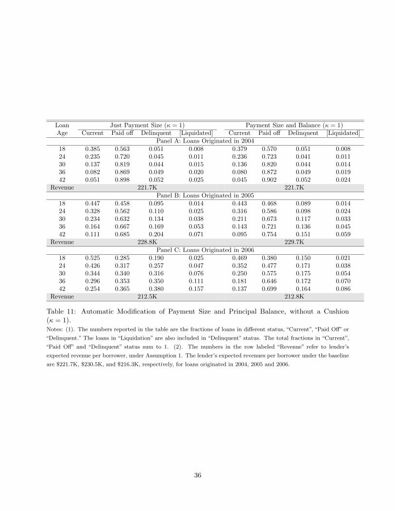
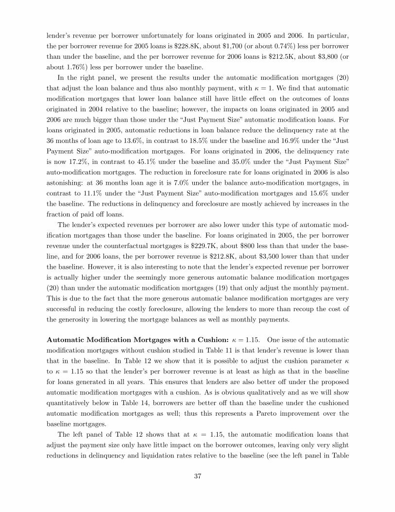
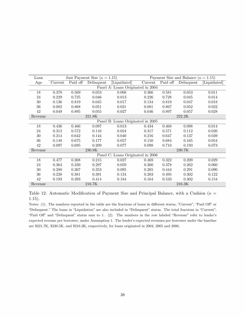
predicts that the delinquency rates for loans originated in 2006 would be about 7% at all loan ages,
and the cumulative liquidation rates would reach 3.3% at 42 months of loan age.
In the right panel, we see that adding the additional assumption that the interest rates would
be fixed at the initial teaser rates of the ARMs for the total duration of the loan only generates
rather small effect. Comparing with the results in the left panel, we find that making the mortgages
of fixed rates rather than of adjustable rates makes the loans more likely to be paid off for young
loans originated in 2004 and 2005 and all loans originated in 2006. Delinquency rates are slightly
lower for loans originated in 2005 and 2006 at all ages, and for older loans originated in 2004. For
loans originated in 2004, the delinquency rates do not change much when the loans are young.
30
Loan h̃t = h0 h̃t = h0 & FRMAge Current Paid off Delinquent [Liquidated] Current Paid off Delinquent [Liquidated]
Table 7: Role of Housing Prices and the Interaction with the Interest Rate Resets.Notes: (1) In the left panel, we assume that the housing price stayed unchanged from that at the loan origination;
in the right panel, we assume in addition that all the ARMs were converted to FRMs with interest rate fixed at the
initial teaser rate of the corresponding ARMs. (2) The numbers reported in the table are the fractions of loans in
different status, “Current”, “Paid Off” or “Delinquent.” The loans in “Liquidation” are also included in “Delinquent”
status. The total fractions in “Current”, “Paid Off” and “Delinquent” status sum to 1.
Loan ∆Unrt = ∆Unr0
Age Current Paid off Delinquent [Liquidated]Panel A: Loans Originated in 2004
Table 8: Role of Labor Market Conditions.Note: The numbers reported in the table are the fractions of loans in different status, “Current”, “Paid Off” or
“Delinquent.” The loans in “Liquidation” are also included in “Delinquent” status. The total fractions in “Current”,
Table 10: Impacts of Traditional Monetary Policy: Setting the Libor Rate to Zero.Note: The numbers reported in the table are the fractions of loans in different status, “Current”, “Paid Off” or
“Delinquent.” The loans in “Liquidation” are also included in “Delinquent” status. The total fractions in “Current”,
“Paid Off” and “Delinquent” status sum to 1.
Also note that as reported in Table 9, in the data margin rates and lifetime floor rates were high
and Libor rates were already low for 2006 loans, thus setting the Libor rate to zero had little effect
on loans originated in 2006. Therefore, the results in Table 10 suggests that setting the Libor rate
at zero would reduce the mortgage pay off rates of almost all loans; however, mortgage delinquency
rates and liquidation rates change little.
7.2.2 Automatic Loan Modification Contingent on Housing Price Index, with a“Cush-
ion”
If a housing price downturn leads to massive default rates, then one way to mitigate this prob-
lem is to link the mortgage monthly payment to the current house price index. Caplin et al. (2007),
Shiller (2008), Mian and Sufi (2014), and Kung (2015) have suggested that such “continuous work-
out mortgages” might have reduced the mortgage default and foreclosure. Piskorski and Tchistyi
(2010, 2011) show that the optimal mortgage contracts in the presence of stochastic house price
appreciation or uncertain income and uncertain mortgage rates all have some forms loss sharing
between borrowers and lenders such as balance or interest rate reduction when house price declines
or when income decreases or interest rates jump. In their model, interest rates are exogenous and
the optimal plan involves a complex home equity line. We consider two different automatic loan
modification schemes in this subsection.30
30Kung (2015) studies the general equilibrium effect of “continuous workout mortgage” on housing price and mort-gage interest rates. Borrowers in his model are only allowed to make the current monthly payment or to refinance,i.e., delinquency and foreclosure are not focus of his paper.
33
Modification of Monthly Payments Only. We first consider the case in which only the
monthly payment amount is automatically modified as housing prices change. Specifically, de-
note P̃t as the modified monthly payment at period t, and Pt as the monthly payment amount in
the absent of modification according to the original loan. Let ht and h0 denote the housing price
index at period t and at origination respectively. The first counterfactual we consider assumes that
the monthly payment will be automatically modified from Pt to P̃t as follows:
P̃t = Pt ×min
{1, κ× ht
h0
}, where κ ≥ 1, (19)
while the principal balance is not adjusted.31 In (19), the parameter κ ≥ 1 can be used to adjust
how much cushion is afforded to the seller in terms of housing price declines before the automatic
modification of monthly payments (and loan balance below) is activated. We refer to κ as the
“cushion parameter”: the higher κ is, the more housing price decline is required to trigger the
automatic modification. For example, as we will experiment below, when κ = 1.15, the housing
price would have to decline by 13% (≈ 1 − 1/κ) from that at the loan origination before monthly
payment is reduced.
Modification of Principal Balance (and Monthly Payments Too) In the second counter-
factual, we assume that
B̃ALt = BALt ×min
{1, κ× ht
h0
}, (20)
where as in (19), κ ≥ 1 is the cushion parameter. Because monthly payment is proportional to
principal balance, as we showed in (2), the automatic modification of principal balance will also
automatically adjust the monthly payment.32
A key feature of the automatic modification mortgages of both forms (19) and (20) is that
modifications are triggered by the housing price declines alone, not at all by the delinquency status
of the borrowers, which are subject to potential strategic behavior by borrowers. This feature
distinguishes from the automatic modification from the stochastic loan modification of the form as
modeled in Section 3.3.
In this subsection, we are also interested in evaluating the impact of alternative mortgage
contracts on the revenue of the lenders. For this purpose, we make the following assumption:33
Assumption 1. Upon foreclosure, the lender receives 75 percent of the house value.
It is worth making three observations. First, the baseline corresponds to the case of κ = +∞,i.e., the monthly payment actually never deviates from those in the baseline. Second, everything
else equal, as long as κ ≥ 1 the borrower is always made better off under both (19) and (20) than
under the baseline in expectation. The closer κ is to 1, the easier that housing price decline triggers
31Stochastic loan modification of the form as modeled in Section 3.3 stays as in the baseline in the counterfactualexperiments in this subsection.
32This is akin to “partially shared appreciation mortgage” considered in Kung (2015).33Campbell, Giglio, and Pathak (2011) find that the average discount of a house value for foreclosures is about 27
percent.
34
reduction in monthly payment under (19), or both loan balance and monthly payment under (20),
and thus the better off the borrowers are.
Third, changes in the cushion parameter κ in the automatic modification mortgages (19) and
(20) have two effects. First, different values of κ affects the borrowers’ payment behavior, resulting
in different levels of delinquency and liquidation. Intuitively, and as we will show below, the
closer κ is to 1, the smaller is the fraction of mortgages that are liquidated, and thus the smaller
the social surplus destruction in the 25% loss of the house value in foreclosure (see Assumption
1). Second, κ affects how the surplus from the reduction in foreclosure is shared between the
borrowers and the lender. When κ is closer to 1, while it is true that the automatic modification
mortgages (19) and (20) prevents more foreclosure, the lender receives a smaller share of the surplus
because the foreclosure reduction is achieved solely by the lender reducing monthly payment and/or
principals. At higher values of the cushion parameter κ, the borrower will also share some of the
“sacrifices” for reduction in foreclosure as smaller declines in housing prices would not trigger the
automatic reduction. As a result, while the borrowers’ ex ante expected value under automatic
modification mortgages is always higher than that in the baseline, and decreasing in κ, the lender’s
expected revenue is non-monotonic in κ. In particular, to the extent that it is important that
lenders voluntarily adopt the automatic modification mortgages of the form (19) or (20), we would
like to explore whether there are values of κ that both the borrowers and lenders are better off
than the baseline. Otherwise, we would expect that lenders would have to raise interest rates to
compensate for their revenue loss.
Automatic Modification Mortgages without a Cushion: κ = 1. In Table 11 we present the
results from counterfactual simulations under automatic modification mortgages, without a cushion,
i.e., when κ = 1. We should emphasize that this version of automatic modification corresponds to
most of what has been studied in the literature.34
In the left panel, we present the results under the automatic modification mortgages (19) that
adjust payment sizes only, with κ = 1. We find that the automatic modification mortgages only
slightly reduce the delinquency and foreclosure rates for loans originated in 2004 and 2005; however,
the delinquency and foreclosure rates are significantly reduced for loans originated in 2006. The
delinquency rate for 2006 loans under the “just payment size” automatic modification mortgages is
reduced from 45.1% under the baseline to 35.0% at 36 months loan age, and the liquidation rate
is lowered from 15.6% to 11.1% at 36 months of loan age and from 21.6% to 15.7% at 42 months
of loan age. As we mentioned earlier, it is important to know how such automatic modification
mortgages might affect lender’s revenues. We also calculate lenders’ revenue as the present value
of the borrower’s expected payment. If a borrower prepays, his payment in that period will just
be the remaining mortgage balance. If a borrower’s house is liquidated, we assume that the lender
receives 75 percent of the estimated current house value as stated in Assumption 1. As stated in the
notes for Table 11, the lender’s revenues per borrower under the baseline are $221.7K, $230.5K, and
$216.3K, respectively, for loans originated in 2004, 2005, and 2006. Comparing these numbers to
those obtained in Table 11, we see that the automatic modification loans of the form (19) lowers the
34For example, this is the case considered in Kung (2015)’s “partially shared appreciation mortgage.”
35
Loan Just Payment Size (κ = 1) Payment Size and Balance (κ = 1)Age Current Paid off Delinquent [Liquidated] Current Paid off Delinquent [Liquidated]
Table 11: Automatic Modification of Payment Size and Principal Balance, without a Cushion(κ = 1).Notes: (1). The numbers reported in the table are the fractions of loans in different status, “Current”, “Paid Off” or
“Delinquent.” The loans in “Liquidation” are also included in “Delinquent” status. The total fractions in “Current”,
“Paid Off” and “Delinquent” status sum to 1. (2). The numbers in the row labeled “Revenue” refer to lender’s
expected revenue per borrower, under Assumption 1. The lender’s expected revenues per borrower under the baseline
are $221.7K, $230.5K, and $216.3K, respectively, for loans originated in 2004, 2005 and 2006.
36
lender’s revenue per borrower unfortunately for loans originated in 2005 and 2006. In particular,
the per borrower revenue for 2005 loans is $228.8K, about $1,700 (or about 0.74%) less per borrower
than under the baseline, and the per borrower revenue for 2006 loans is $212.5K, about $3,800 (or
about 1.76%) less per borrower under the baseline.
In the right panel, we present the results under the automatic modification mortgages (20)
that adjust the loan balance and thus also monthly payment, with κ = 1. We find that automatic
modification mortgages that lower loan balance still have little effect on the outcomes of loans
originated in 2004 relative to the baseline; however, the impacts on loans originated in 2005 and
2006 are much bigger than those under the “Just Payment Size” automatic modification loans. For
loans originated in 2005, automatic reductions in loan balance reduce the delinquency rate at the
36 months of loan age to 13.6%, in contrast to 18.5% under the baseline and 16.9% under the “Just
Payment Size” auto-modification mortgages. For loans originated in 2006, the delinquency rate
is now 17.2%, in contrast to 45.1% under the baseline and 35.0% under the “Just Payment Size”
auto-modification mortgages. The reduction in foreclosure rate for loans originated in 2006 is also
astonishing: at 36 months loan age it is 7.0% under the balance auto-modification mortgages, in
contrast to 11.1% under the “Just Payment Size” auto-modification mortgages and 15.6% under
the baseline. The reductions in delinquency and foreclosure are mostly achieved by increases in the
fraction of paid off loans.
The lender’s expected revenues per borrower are also lower under this type of automatic mod-
ification mortgages than those under the baseline. For loans originated in 2005, the per borrower
revenue under the counterfactual mortgages is $229.7K, about $800 less than that under the base-
line, and for 2006 loans, the per borrower revenue is $212.8K, about $3,500 lower than that under
the baseline. However, it is also interesting to note that the lender’s expected revenue per borrower
is actually higher under the seemingly more generous automatic balance modification mortgages
(20) than under the automatic modification mortgages (19) that only adjust the monthly payment.
This is due to the fact that the more generous automatic balance modification mortgages are very
successful in reducing the costly foreclosure, allowing the lenders to more than recoup the cost of
the generosity in lowering the mortgage balances as well as monthly payments.
Automatic Modification Mortgages with a Cushion: κ = 1.15. One issue of the automatic
modification mortgages without cushion studied in Table 11 is that lender’s revenue is lower than
that in the baseline. In Table 12 we show that it is possible to adjust the cushion parameter κ
to κ = 1.15 so that the lender’s per borrower revenue is at least as high as that in the baseline
for loans generated in all years. This ensures that lenders are also better off under the proposed
automatic modification mortgages with a cushion. As is obvious qualitatively and as we will show
quantitatively below in Table 14, borrowers are better off than the baseline under the cushioned
automatic modification mortgages as well; thus this represents a Pareto improvement over the
baseline mortgages.
The left panel of Table 12 shows that at κ = 1.15, the automatic modification loans that
adjust the payment size only have little impact on the borrower outcomes, leaving only very slight
reductions in delinquency and liquidation rates relative to the baseline (see the left panel in Table
37
Loan Just Payment Size (κ = 1.15) Payment Size and Balance (κ = 1.15)Age Current Paid off Delinquent [Liquidated] Current Paid off Delinquent [Liquidated]
Table 12: Automatic Modification of Payment Size and Principal Balance, with a Cushion (κ =1.15).Notes: (1). The numbers reported in the table are the fractions of loans in different status, “Current”, “Paid Off” or
“Delinquent.” The loans in “Liquidation” are also included in “Delinquent” status. The total fractions in “Current”,
“Paid Off” and “Delinquent” status sum to 1. (2). The numbers in the row labeled “Revenue” refer to lender’s
expected revenue per borrower, under Assumption 1. The lender’s expected revenues per borrower under the baseline
are $221.7K, $230.5K, and $216.3K, respectively, for loans originated in 2004, 2005 and 2006.
38
6) for loans originated in all years, though the lender’s revenue also increase slightly relative to
the baseline. However, the right panel shows that automatic modification mortgages that reduce
the mortgage balance when the housing price declines by about 13 percent (= 1 − 1/1.15) are
able to achieve moderate reductions in delinquency and liquidation rates for loans originated in
2005, and more sizable reductions for loans originated in 2006. Specifically, we find that under the
automatic modification mortgages that reduce balance with κ = 1.15, for loans originated in 2005,
the delinquency rate at 42 months of loan age decreases from 21.7% in the baseline to 19.3%, and
the liquidation rate is reduced from 8.2% in the baseline to 7.3%; for loans originated in 2006, the
delinquency rate at 43 months of loan age decreases from 47.4% in the baseline to 30.2% and the
liquidation rate is reduced from 21.6% in the baseline to 15.4%. At the same time, the lender’s per
borrower revenue is at least as high as that in the baseline for all years. Even though the reductions
in delinquency and liquidation rates under auto-modification mortgages with a cushion parameter
κ = 1.15 is not as large as those without a cushion, it should be noted that the lenders would
not have to increase their interest rate under the cushioned auto-modification mortgages. It is also
worth noting that borrowers are benefiting from the automatic modification mortgages regardless of
whether they are eventually delinquent or liquidated, since one important feature of the automatic
modification mortgages is that modifications are triggered by the housing price declines, not at all
by the delinquency status of the borrowers, which are subject to potential strategic behavior by
borrowers.
7.3 What if the Lender Can Commit Not to Modify Any Loans?
In this subsection, we consider a different counterfactual: what if the lender can commit not to
modify any loans? This counterfactual can shed light on whether borrowers’ strategic defaults, in
order to receive loan modification, played any role in the observed delinquency and liquidation. As
we will argue below, it will also shed light on why the fraction of loans that received modification
(only 0.26%) during the housing crisis was so low.
To implement this counterfactual, we consider two scenarios depending on whether the lender
would replace each loan modification observed in the data by either the alternative of “waiting and
do nothing” or the alternative of “liquidation.” The results are presented in Table 13.
In the left panel, we assume that the lenders replace all modifications in the data by liquidation
instead. We find that, with the additional threat of foreclosure, borrowers are much less likely
to default on their mortgages than the baseline and this effect is particularly strong for loans
originated in 2005 and 2006; and much higher fraction of loans are paid off. Because of the now
higher probability of liquidation, although liquidation rates come down for all loans the magnitude
of the reductions of liquidation rates is much smaller. Surprisingly, the lender’s per borrower
revenues under this counterfactual policy are respectively $224.6K, $240.4K, and $233.2K for loans
originated in 2004, 2005 and 2006, which are respectively 1.3%, 4.3% and 7.8% higher than their
counterparts under the baseline. The increases in lender revenue are mainly due to more borrowers
paying off their loans (despite prepayment penalty for most of the loans), and less delinquency.
In the right panel, we assume that the lenders replace all modifications in the data by “waiting.”
39
Loan No Modification, More Liquidation No Modifcation, More WaitingAge Current Paid off Delinquent [Liquidated] Current Paid off Delinquent [Liquidated]
Table 13: Automatic Modification of Payment Size and Principal Balance, without a Cushion(κ = 1).Notes: (1). The numbers reported in the table are the fractions of loans in different status, “Current”, “Paid Off” or
“Delinquent.” The loans in “Liquidation” are also included in “Delinquent” status. The total fractions in “Current”,
“Paid Off” and “Delinquent” status sum to 1. (2). The numbers in the row labeled “Revenue” refer to lender’s
expected revenue per borrower, under Assumption 1. The lender’s expected revenues per borrower under the baseline
are $221.7K, $230.5K, and $216.3K, respectively, for loans originated in 2004, 2005 and 2006.
40
We find that mortgage delinquency rates are also lower than the baseline, though the reduction is
less pronounced than in the previous case where lenders replace modification by liquidation. As
in the previous case, borrowers pay off more often than in the baseline when there is no prospect
of loan modification. Note that the liquidation rate under this counterfactual policy is actually
higher than that in the baseline for loans originated in 2006; after all, waiting and doing nothing
by the lender in place of modification will still raise borrowers’ months in delinquency, eventually
increasing the probability of foreclosure. It may seem somewhat surprising that borrowers will be
less likely to default when the lender commits not to modify any loans. The reason is actually
quite simple. The ex ante value of being delinquent is a lot lower without any possibilities to get
their loans modified; and as the months in delinquency rise, the house will eventually be foreclosed.
So the value of being delinquent decreases substantially without modification. In other words, the
presence of modification possibility led some borrowers to delinquency in the hopes of getting their
interest rates reduced.
Again, it is interesting to note that the lenders’ expected per borrower revenues under this
counterfactual policy are $224.4K, $238.8K and $230.0K respectively for loans originated in 2004,
2005, and 2006, which are respectively 1.2%, 3.6% and 6.3% higher than their counterparts under
the baseline.
Discussion. The counterfactual results reported in Table 13 suggest that the lenders would have
been able to raise their expected revenue if they were able to commit not to offer any modification
at all. Similarly, results reported in Table 12 show that the lenders could also have raised their
expected revenue if they could commit to automatically modify the loan balances whenever the
housing prices decline by more than 13%. In reality, however, as we mentioned in the discussions
following Table 1, only 5.24% of the loans were modified. The key puzzle is what explains this small
presence of the loan modification? Table 13 suggests that the lenders’ revenue would have been
higher if they did not offer any loan modification; yet Table 12 and many commentators suggest
that they should have offered more modification and more automatic modification.
We would like to point out that the results in Tables 13 and 12 are both predicated on the
lenders having the ability to commit: in the case of Table 13 the lenders need to commit never to
offer modification to any borrower regardless of his circumstances; and in the case of Table 12 the
lender needs to be able to commit to automatically reduce the loan balance whenever the housing
prices decline by more than 13% regardless of whether the borrower has shown any difficulty in
making the payments. In reality the lenders do not have the commitment power. We believe that
the lack of commitment power is an important contributor to understand the lender behavior and
will further investigate this issue in future research.
7.4 Quantitative Assessment of the Impact on Borrowers’ Ex Ante Expected
Welfare
In Table 14 we summarize the borrowers’ average expected welfare evaluated at the loan age
of month 1 under the baseline and different counterfactual scenarios. It shows that borrowers are
41
Loan Year of Origination 2004 2005 2006Baseline 34.859 34.819 33.293Automatic Modification, Just Payment (κ = 1) 35.007 35.796 35.768Automatic Modification, Both Payment and Balance (κ = 1) 35.014 35.836 37.703Automatic Modification, Just Payment (κ = 1.15) 34.887 35.111 33.881Automatic Modification, Both Payment and Balance (κ = 1.15) 34.898 35.363 35.513No Modification, More Liquidation 32.576 32.076 30.304No Modification, More Waiting 32.867 32.472 30.556
Table 14: Borrower’s Ex Ante Expected Welfare Under the Baseline and Different CounterfactualScenarios.Notes: (1) Units are in $1, 000. (2) The borrowers’ expected welfare evaluated at loan age 1. The expected utility of
the borrower under different scenarios is converted into dollar units via dividing the utility by the estimated coefficient
for monthly payment in the utility function.
always better off under the automatic modification mortgages of both forms (19) and (20), and with
or without cushion. As expected, borrowers are better off under automatic modification mortgages
that adjust both payment and balance than under automatic modification mortgages that adjust
only the payment, and also the borrowers are better off when the automatic adjustment is triggered
without a cushion (when κ = 1) than with a cushion (when κ = 1.15). We also find that borrowers
are significantly worse off if the lenders commit not to offer any loan modifications.
8 Conclusion
One important characteristic of the recent mortgage crisis is the prevalence of subprime mort-
gages with adjustable interest rates and their high default rates. In this paper, we present a
dynamic structural model of subprime adjustable-rate mortgage (ARM) borrowers making pay-
ment decisions taking into account possible consequences of different degrees of delinquency from
their lenders. We empirically implement the model using unique data sets that contain information
on borrowers’ mortgage payment history, their broad balance sheets, and lender responses.
Our investigation of the factors that drive borrowers’ decisions reveals that subprime ARMs
are not all alike. For loans originated in 2004 and 2005, which preceded the peak of the housing
prices, the interest rate resets associated with ARMs, as well as the housing and labor market
conditions were not as important in borrowers’ delinquency decisions as in their decisions to pay off
their loans. For loans originated in 2006, interest rate resets, housing price declines, and worsening
labor market conditions all contributed importantly to their high delinquency rates. Counterfactual
policy simulations further suggest that even if the Libor rate could be lowered to zero by aggressive
monetary policies, it would have a limited effect on reducing the delinquency rates. We also
examine the effectiveness of automatic modification mortgages under which the monthly payment
or the principal balance of the loans are automatically reduced when housing prices decline. We
show that such alternative mortgage designs can be effective in reducing both delinquency and
foreclosure; and importantly, we find that automatic modification mortgages with a cushion, which
will trigger the monthly payment or principal balance reductions only when housing price declines
exceed a certain percentage may result in a Pareto improvement in that borrowers and lenders are
42
both made better off than under the baseline, with a much lower delinquency and foreclosure rates.
Our counterfactual analysis also suggests that limited commitment on the part of lenders to
loan modification policies may be an important reason for the relatively small rate of modifications
observed during the housing crisis. In future research, we plan to model lender behavior explicitly,
so that we can have a better understanding of what is the nature of the lender’s lack of commit-
ment issue, and how policies may be designed to alleviate the lender’s lack of commitment power
problem. It is also important to consider the general equilibrium effects of alternative mortgages
on the housing market, both on the mortgage interest rates the lenders may charge and on the
housing market prices, particularly taking into account the spillover effects on property prices due
to foreclosed properties.
References
[1] Adelino, Manuel, Kristopher S. Gerardi and Paul S. Willen (2013). “Why Don’t Lenders Rene-
gotiate More Home Mortgages? Redefaults, Self-Cures and Securitization.” Journal of Mone-
tary Economics, 60(7): 835–853.
[2] Agarwal, Sumit, Gene Amromin, Itzhak Ben-David, Souphala Chomsisengphet, and Douglas
Evanoff (2011). “Market-Based Loss Mitigation Practices for Troubled Mortgages Following
the Financial Crisis,” Federal Reserve Bank of Chicago Working Paper 2011-03.
Table A4: Lenders’ Decisions for Loans in Categories 1-3 (Florida, origination year: 2006).Notes: (1). Results are from logit Regressions where the dependent variable is a dummy for loan modification.
(2).***, ** and * denote statistical significance at 1%, 5% and 10% respectively.
50
Modification LiquidationVariable coeff. s.d. coeff. s.d.Current Credit Score 0.0000 0.0003 0.0006*** 0.0001Income at origination ($1000) -0.1178*** 0.0009 0.0024*** 0.0005Loan-to-value -1.8278*** 0.5408 4.6127*** 0.5897Loan-to-value at origination 0.5969*** 0.1636 -1.1419 0.1248Deviation in local unemp. rates (%) 0.3224 0.0528 - 0.0987 0.0757Current monthly payment ($1000) 0.0141 0.0816 -0.1620*** 0.0512Initial monthly payment ($1000) 0.1288 0.0830 0.0703 0.0514Loan age (months) 0.2019*** 0.0174 -0.1291*** 0.0109Loan age squared -0.0038*** 0.0004 0.0026*** 0.0002Months of delinquency -0.3988*** 0.1261 0.6474*** 0.0921Months of delinquency squared 0.0132** 0.0048 -0.0170*** 0.0320Loan to value ratio x Months of delinquency 0.4045*** 0.1061 -0.4214*** 0.0866Loan to value ratio x Months of delinquency squared -0.0138** 0.0046 0.0101*** 0.0032Dummy for full documentation 0.2027*** 0.0323 -0.0715*** 0.0216Change in unemp rates x number of late payments -0.0138 0.0107 -0.0156 0.0107Change in unemp rates x number of late payments2 -0.0000 0.0005 - 0.0008** 0.0004Dummy for 4-month delinquency 0.6252 0.4113 -3.8769*** 0.2652Dummy for 5-month delinquency 0.73538** 0.3514 -2.8718*** 0.2029Dummy for 6-month delinquency 0.4998 0.2973 -2.5894*** 0.1679Dummy for 7-month delinquency 0.6295** 0.2472 -1.8006*** 0.1295Dummy for 8-month delinquency 0.4306** 0.2039 -1.1820*** 0.1003Dummy for 9-month delinquency 0.3777** 0.1661 -0.5726*** 0.0765Dummy for 10-month delinquency 0.2491 0.1366 -0.2683*** 0.0597Dummy for 11-month delinquency 0.1405 0.1162 -0.0699 0.0478Constant -5.6849*** 0.8695 -6.0277*** 0.6546Number of observations 304,984Pseudo-R2 0.0933
Table A5: Lenders’ Decisions on Category 4 Loans (Florida, origination year: 2006).Notes: (1). Results are from multinomial logit Regressions where the alternatives are modification, liquidation and
waiting (omitted). (2). ***, ** and * denote statistical significance at 1%, 5% and 10% respectively.
51
ModificationVariable coeff. s.d.Log (initial interest rate) 0.4131*** 0.0270Log (margin rate) 0.2042*** 0.0141Initial balance ($1000) 0.0018*** 0.0006Remaining balance ($1000) -0.0022** 0.0005Current Credit Score -0.00004** 0.00002Income at origination 0.0004*** 0.0001Loan-to-value ratio 0.2583 *** 0.0203Loan-to-value ratio at origination -0.1266*** 0.0200Local unemployment rate deviation -0.0285*** 0.0016Loan age (months) -0.0103*** 0.0025Loan age squared 0.0003*** 0.0001Full documentation 0.0463*** 0.0042Months of delinquency -0.0209*** 0.0016Months of delinquency squared 0.0001 0.0001Loans originated in Arizona -0.0176 0.0106Loans originated in California -0.0136 0.0098Loans originated in Florida -0.0197** 0.0098Constant 0.7171*** 0.0719Number of observations 18,646Pseudo-R2 0.2738
Table A6: Lenders’ Decisions on Modified Interest rates (origination year: 2006).Note: ***, ** and * denote statistical significance at 1%, 5% and 10% respectively.