The Dynamics of Adjustable-Rate Subprime Mortgage Default: A Structural Estimation * Hanming Fang † You Suk Kim ‡ Wenli Li § May 27, 2015 Abstract One important characteristic of the recent mortgage crisis is the prevalence of subprime mortgages with adjustable interest rates and their high default rates. In this paper, we build and estimate a dynamic structural model of adjustable-rate mortgage defaults using unique mortgage loan level data. The data contain detailed information not only on borrowers’ mortgage payment history and lender responses but also on their broad balance sheet. Our structural estimation suggests that the factors that drive the borrower delinquency and fore- closure differ substantially by the year of loans’ origination. For loans that originated in 2004 and 2005, which precedes the severe downturn of the housing and labor market conditions, the interest rate resets associated with ARMs, as well as the housing and labor market condi- tions do not seem to be important factors for borrowers’ delinquency behavior, though they are important factors that determine whether the borrowers would pay off their loans (i.e., sell their houses or refinance). However, for loans that originated in 2006, interest rate reset, housing price declines and worsening labor market conditions all contributed importantly to their high delinquency rates. Countefactual policy simulations also suggest that mone- tary policies in the most optimistic scenario might have limited effectiveness in reducing the delinquency rates of 2004 and 2005 loans, but could be much more effective for 2006 loans. Interestingly, we found that automatic modification loans in which the monthly payment and principal balance of the loans are automatically reduced when housing prices decline can reduce delinquency and foreclosure rates, and significantly so for 2006 loans, without having much a negative impact on lenders’ expected income. * Preliminary and Incomplete. All comments are welcome. The views expressed are those of the authors and do not necessarily reflect those of the Board of Governors of the Federal Reserve, the Federal Reserve Bank of Philadelphia, or the Federal Reserve System. † Department of Economics, University of Pennsylvania, 3718 Locust Walk, Philadelphia, PA 19104 and the NBER. Email: [email protected]‡ Division of Research and Statistics, Board of Governors of the Federal Reserve System. Email: [email protected]. § Department of Research, Federal Reserve Bank of Philadelphia. Email: [email protected].
Transcript
The Dynamics of Adjustable-Rate Subprime Mortgage Default:
A Structural Estimation∗
Hanming Fang† You Suk Kim‡ Wenli Li§
May 27, 2015
Abstract
One important characteristic of the recent mortgage crisis is the prevalence of subprime
mortgages with adjustable interest rates and their high default rates. In this paper, we build
and estimate a dynamic structural model of adjustable-rate mortgage defaults using unique
mortgage loan level data. The data contain detailed information not only on borrowers’
mortgage payment history and lender responses but also on their broad balance sheet. Our
structural estimation suggests that the factors that drive the borrower delinquency and fore-
closure differ substantially by the year of loans’ origination. For loans that originated in 2004
and 2005, which precedes the severe downturn of the housing and labor market conditions,
the interest rate resets associated with ARMs, as well as the housing and labor market condi-
tions do not seem to be important factors for borrowers’ delinquency behavior, though they
are important factors that determine whether the borrowers would pay off their loans (i.e.,
sell their houses or refinance). However, for loans that originated in 2006, interest rate reset,
housing price declines and worsening labor market conditions all contributed importantly
to their high delinquency rates. Countefactual policy simulations also suggest that mone-
tary policies in the most optimistic scenario might have limited effectiveness in reducing the
delinquency rates of 2004 and 2005 loans, but could be much more effective for 2006 loans.
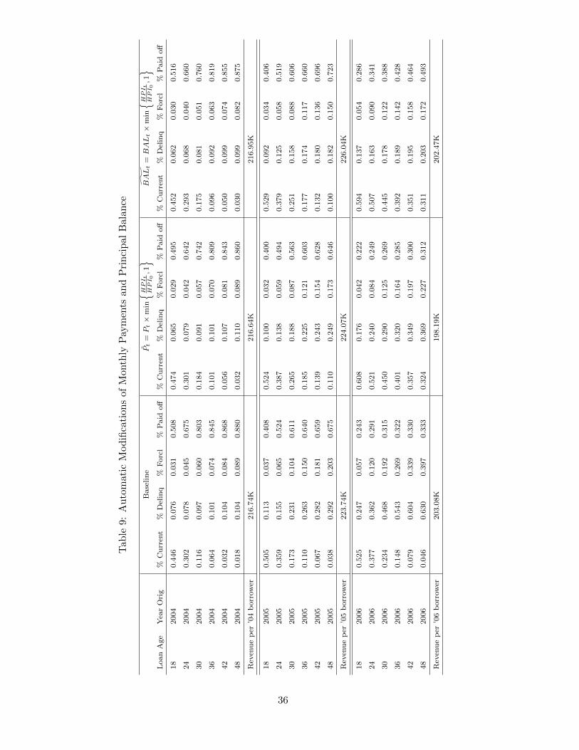
Interestingly, we found that automatic modification loans in which the monthly payment
and principal balance of the loans are automatically reduced when housing prices decline can
reduce delinquency and foreclosure rates, and significantly so for 2006 loans, without having
much a negative impact on lenders’ expected income.
∗Preliminary and Incomplete. All comments are welcome. The views expressed are those of the authors anddo not necessarily reflect those of the Board of Governors of the Federal Reserve, the Federal Reserve Bank ofPhiladelphia, or the Federal Reserve System.†Department of Economics, University of Pennsylvania, 3718 Locust Walk, Philadelphia, PA 19104 and the
NBER. Email: [email protected]‡Division of Research and Statistics, Board of Governors of the Federal Reserve System. Email:
The collapse of the subprime residential mortgage market played a crucial role in the recent
housing crisis and the subsequent Great Recession.1 At the end of 2007, subprime mortgages
accounted for about 13 percent of total first-lien residential mortgages outstanding but over half
of total house foreclosures. The majority of the subprime mortgages, by number as well as by
value, had adjustable rates and the fraction of the adjustable-rate subprime mortgages in foreclo-
sure at 17 percent was much higher than the fraction of the fixed-rate subprime mortgages at 5
percent (Frame, Lehnert, and Prescott 2008, Table 1). In response to these developments, many
government policies have been designed and carried out that aimed at changing the incentives
of these borrowers to default.2 Few structural models, however, exist that can guide us in these
efforts especially since most of them have had limited success.3
In this paper, we first develop a dynamic structural model to study the various incentives
adjustable-rate subprime borrowers have to default and how these incentives change under differ-
ent policies. Our study focuses on the period between the time when either a mortgage is granted
and the time when the mortgage is repaid (including refinance), or the house is foreclosed, or
the end of the sample period. More specifically, at each period, a borrower decides whether to
repay the loan (and be current) or not repay the loan (and stay in various delinquent status),
taking as given lender’s possible responses which include various loss-mitigation practices such
1There is no standard definition of subprime mortgage loans. Typically, they refer to loans made to borrowerswith poor credit history (e.g., a FICO score below 620) and/or with a high leverage as measured by either thedebt-to-income ratio or the loan-to-value ratio. For the data used in this paper, subprime mortgages are definedas those in private-label mortgage-backed securities marketed as subprime, as in Mayer, Pence, and Sherlund(2009).
2To name a few of such programs, the FHASecure program approved by Congress in September 2007; the HopeNow Alliance program (HOPENOW) created by then-Treasury Secretary Henry Paulson in October 2007; Hopefor Homeowners refinancing program passed by Congress in the spring 2008; Making Home Affordable (MHA)initiative in conjunction with the Home Affordable Modification Program (HAMP) and the Home AffordableRefinance Program (HARP) launched by the Obama administration in March 2009 (HAMP). See Gerardi and Li(2010) for more details.
3Over the first two and a half years, HARP refinancing activity remained subdued relative to model-basedextrapolations from historical experience. From its inception to the end of 2011, 1.1 million mortgages refi-nanced through HARP, compared to the initial announced goal of three to four million mortgages. In De-cember, HARP 2.0 was introduced and HARP refinance volume picked up, reaching 3.2 million by June 2014.http://www.fhfa.gov/AboutUS/Reports/Pages/Refinance-Report-February-2014.aspx. Similarly, HAMP was de-signed to help as many as 4 million borrowers avoid foreclosure by the end of 2012. By February 2010, oneyear into the program, only 168,708 trial plans had been converted into permanent revisions. Through January2012, a population of 621,000 loans had received HAMP modifications. See http://www.treasury.gov/resource-center/economic-policy/Documents/HAMPPrincipalReductionResearchLong070912FINAL.pdf
1
as mortgage modification, liquidation, and waiting (i.e., doing nothing). Relative to the existing
structural models on mortgage defaults which we review below, our theoretical framework has
the two key distinguishing features: first, in our model default is not the terminal event, and
second, besides liquidation we also consider lenders’ various loss mitigation practices such as
loan modification.
We then empirically implement our model using unique mortgage loan level data. Our data
not only contains detailed information on borrowers’ mortgage payment history and lenders’
responses, but also detailed credit bureau information (from TransUnion) about borrowers’
broader balance sheet and income. We are thus one of the first to utilize borrowers’ credit
bureau information to understand their mortgage payment decisions.4 To track movements in
home prices and local employment situation, we further merge our data with zip code level home
price indices and county level unemployment rates.
Three main forces drive adjustable-rate mortgage (ARM) borrowers’ mortgage payment de-
cisions: changes in home equity, changes in income, and changes in monthly mortgage payment.
Borrowers with negative home equity have little financial gains from continuing with their mort-
gage payments especially when they do not expect house prices to recover and when costs
associated with defaults and foreclosures are low. Changes in incomes and expenses including
monthly mortgage payments affect borrowers’ liquidity position. In principal, borrowers can
refinance their mortgages to lower interest rates or sell their houses to improve their liquidity
positions, but these options may not be available in the presence of declining house prices, in-
creasing unemployment rates, rising interest rates, and/or tightened lending standards. As a
result, these constrained borrowers have no choice but to default on their mortgages. To arrive
at the relative importance of these different drivers of default, we analyze our structurally es-
timated model under various counterfactual scenarios. Our structural estimation suggests that
the factors that drive the borrower delinquency and foreclosure differ substantially by the year
of loans’ origination. For loans that originated in 2004 and 2005, which precedes the severe
downturn of the housing and labor market conditions, the interest rate resets associated with
ARMs, as well as the housing and labor market conditions do not seem to be important factors
for borrowers’ delinquency behavior, though they are important factors that determine whether
the borrowers would pay off their loans (i.e., sell their houses or refinance). However, for loans
that originated in 2006, interest rate reset, housing price declines and worsening labor market
conditions all contributed importantly to their high delinquency rates.
Our counterfactual policy simulations suggest that monetary policies in the most optimistic
scenario might have limited effectiveness in reducing the delinquency rates of 2004 and 2005
4Elul, Souleles, Chomsisengphet, Glennon, and Hunt (2010) also use credit bureau information to study mort-gage default decisions in their empirical analysis.
2
loans, but could be much more effective for 2006 loans. Interestingly, we found that automatic
modification loans in which the monthly payment and principal balance of the loans are au-
tomatically reduced when housing prices decline can reduce delinquency and foreclosure rates,
and significantly so for 200 loans, without having much a negative impact on lenders’ expected
income.
There are several structural models on mortgage defaults and foreclosures. None of them,
however, captures lenders’ decisions beyond setting interest rates and liquidation despite the
use of other loss-mitigation tools such as mortgage modification in practice. Furthermore, they
all treat default as a terminal event that leads to liquidation with certainty. We briefly review
several closely related papers. Bajari, Chu, Nekipelov, and Park (2013) is the closest in spirit
and methodology to our paper. Both papers provide and estimate using micro data dynamic
structural models to understand borrowers’ behavior and to conduct policy analyses. There are,
however, key differences in addition to the two mentioned previously. First, we estimate bor-
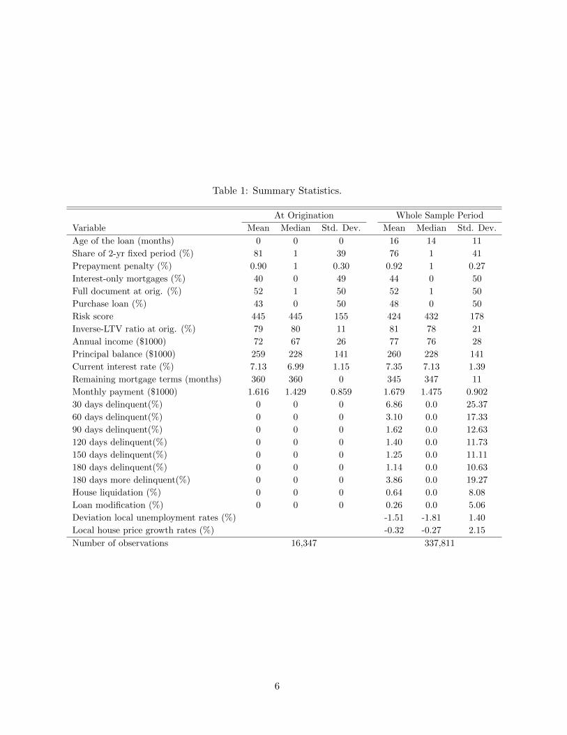
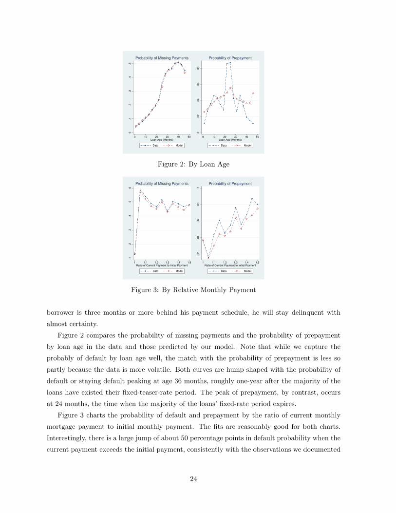
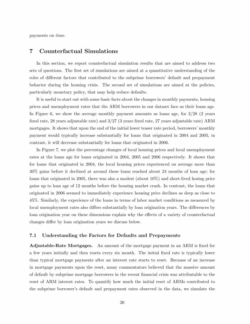
Deviation local unemployment rates (%) -1.51 -1.81 1.40
Local house price growth rates (%) -0.32 -0.27 2.15
Number of observations 16,347 337,811
6
is 14 months. At origination, 81 percent of the sample are loans with two-year fixed-rates.
Through the sample period, however, 76 percent of the sample are loans originated with two-
year initial fixed-rate period indicating that more of those loans have terminated. over 90 percent
of the loans have prepayment penalty. About 40 percent of the mortgages at origination are
interest-only mortgages and the fraction becomes slightly higher for the whole sample. About
half of the mortgages have full documentation both at the origination and through the sample
period. While about 43 percent of the mortgages are purchase loans at the origination, the
ratio increases to about 48 percent indicating that purchase loans are less likely to default than
refinance loans. The risk scores are estimated by TransUnion. They range between 150 and
950 with a high score indicating low risk. Consistent with being subprime, mortgage borrowers
in the sample all have relatively low risk scores, averaging about 445 at origination, and the
scores deteriorate somewhat as the loans age suggesting that the relatively less riskier borrowers
may have refinanced their loans and therefore left our sample. Additionally, both the average
and the mean mortgage loan-to-value ratios exceed 100 at origination and they do not change
much as the loans aged.6 The annual household income estimated by TransUnion average about
$72,000 at origination and $77,000 dynamically. The fact that both mean and median income
are higher in the dynamic sample than at origination suggests that mortgage loans from low
income households are terminated earlier in our sample. Loan balances average $259,000 at
origination with a median of $228,000. These numbers are not very different from their dynamic
counterparts suggesting that borrowers do not make much loan payments during our sample
period. The mortgage interest rates average about 7.13 percent at origination with a median of
6.99 percent. Interestingly, dynamically both the mean and median mortgage interest rates are
higher by 20 and 15 basis points, respectively, as many of these adjustable-rate mortgages reset
to higher rates after the initial fixed-rate period expires. Unemployment rates tend to be lower
than their local averages. Local house prices, on the other hand, all depreciate.
The two most striking observations emerge from Table 1. First, some mortgages stayed in
delinquency status for a long time without being liquidated. Particularly, in our sample, close to
7 percent of loans are 30-day delinquent, 3 percent are 60-day delinquent, 2 percent are 90-day
delinquent, etc. What is most surprising is that close to 4 percent of the loans are actually over
half a year delinquent. The house liquidation rate, by contrast, is only 0.64 percent. Second,
about 0.26 percent of all mortgage loans are modified by their lenders. This ratio is obviously
much higher if we consider loans that are delinquent. We elaborate the second observation
regarding lenders’ decisions in more details in the next subsection.
6We report inverse mortgage-loan-to-value ratio in Table 1. The reason is because in our estimation we assumethat house prices follow an AR(1) process with a normal distribution. The mortgage loan-to-value ratio, which isthe inverse of a normal random variable, does not have a mean. See the model section for more details.
7
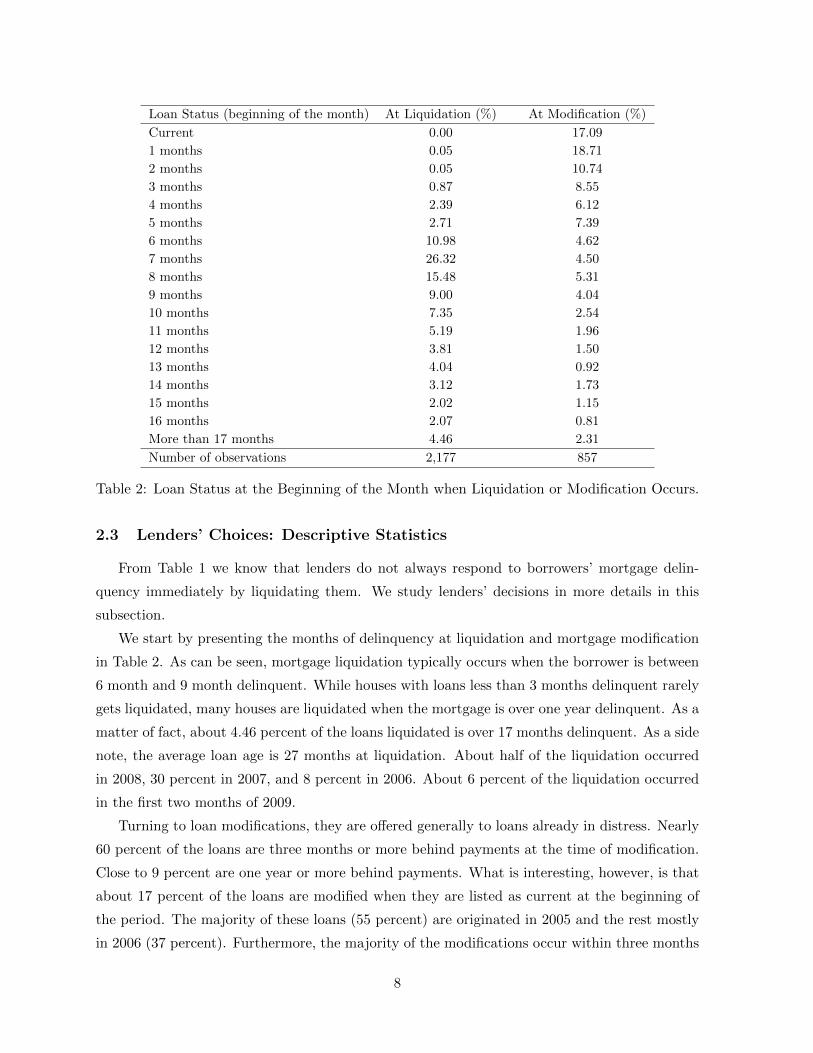
Loan Status (beginning of the month) At Liquidation (%) At Modification (%)
Current 0.00 17.09
1 months 0.05 18.71
2 months 0.05 10.74
3 months 0.87 8.55
4 months 2.39 6.12
5 months 2.71 7.39
6 months 10.98 4.62
7 months 26.32 4.50
8 months 15.48 5.31
9 months 9.00 4.04
10 months 7.35 2.54
11 months 5.19 1.96
12 months 3.81 1.50
13 months 4.04 0.92
14 months 3.12 1.73
15 months 2.02 1.15
16 months 2.07 0.81
More than 17 months 4.46 2.31
Number of observations 2,177 857
Table 2: Loan Status at the Beginning of the Month when Liquidation or Modification Occurs.
2.3 Lenders’ Choices: Descriptive Statistics
From Table 1 we know that lenders do not always respond to borrowers’ mortgage delin-
quency immediately by liquidating them. We study lenders’ decisions in more details in this
subsection.
We start by presenting the months of delinquency at liquidation and mortgage modification
in Table 2. As can be seen, mortgage liquidation typically occurs when the borrower is between
6 month and 9 month delinquent. While houses with loans less than 3 months delinquent rarely
gets liquidated, many houses are liquidated when the mortgage is over one year delinquent. As a
matter of fact, about 4.46 percent of the loans liquidated is over 17 months delinquent. As a side
note, the average loan age is 27 months at liquidation. About half of the liquidation occurred
in 2008, 30 percent in 2007, and 8 percent in 2006. About 6 percent of the liquidation occurred
in the first two months of 2009.
Turning to loan modifications, they are offered generally to loans already in distress. Nearly
60 percent of the loans are three months or more behind payments at the time of modification.
Close to 9 percent are one year or more behind payments. What is interesting, however, is that
about 17 percent of the loans are modified when they are listed as current at the beginning of
the period. The majority of these loans (55 percent) are originated in 2005 and the rest mostly
in 2006 (37 percent). Furthermore, the majority of the modifications occur within three months
8
Variable Reduction No Change∗ Increase
Monthly payment (percentage) 83.41 7.95 8.64
Average change in monthly payment ($)-542
(443)
1
(19)
287
(1,141)
Balance (percentage) 5.41 30.18 64.40
Average change in balance ($)-34,030
(39,603)
-73
(143)
12,248
(11,993)
Interest rate (percentage) 83.11 16.89 0.00
Average change in interest rate (%)-2.980
(1.415)
0.00
(0.00)n/a
Table 3: Terms of Modification.Notes: No change refers to monthly payment change less than 50andtotalloanbalancechangelessthan500. Stan-dard deviations are in parenthesis.
of interest rate reset. These suggest that servicers are aware that these borrowers will default
imminently without mortgage modification.7
Table 3 presents modification terms. The majority of the modification results in more af-
fordable mortgages as 83 percent of them have a reduction in monthly payments of about $542.
However, about 9 percent of the modifications produce higher payments of about $287 on av-
erage. Capitalization of modification is very common with arrearage added to total principal
balance. Indeed over 64 percent of the modified loans have an increase of principal balance of
$12,248 on average. Only 5 percent of the loans have a principal reduction averaging $34,030.
Nonetheless, more than 83 percent of the modified loans have an annualized interest rate reduc-
tion averaging 2.98 percent, leading to reduced monthly payment. No modified loans experience
any interest rate increase. All of the loans are brought into the current status after modification.
3 The Model
The model describes a borrower’s behavior from the time his mortgage is originated until
period T which we specify later. We do not model lenders’ decision but estimate it parameter-
ically, which borrowers take as given. Time is discrete and finite with each period representing
one month. Let xt denote the state vector in period t, which includes time-invariant borrower
and mortgage characteristics such as information collected at mortgage origination and house
location as well as time-varying characteristics such as a mortgage’s delinquency status, interest
rates, local housing market conditions, local unemployment rates, etc.
7Haughwout (2010) documented similar observations but their sample are different from ours as they includefixed rate mortgages, adjustable-rate mortgages that have more than 3 years of fixed period, and mortgages withmaturity not equal to 30 years (Table 3).
9
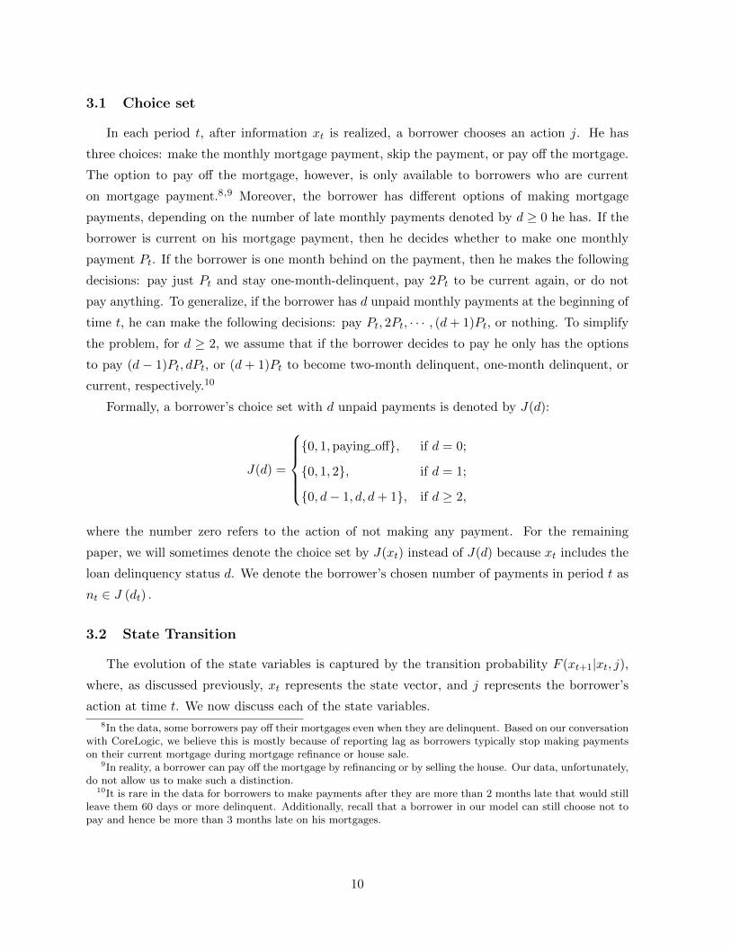
3.1 Choice set
In each period t, after information xt is realized, a borrower chooses an action j. He has
three choices: make the monthly mortgage payment, skip the payment, or pay off the mortgage.
The option to pay off the mortgage, however, is only available to borrowers who are current
on mortgage payment.8,9 Moreover, the borrower has different options of making mortgage
payments, depending on the number of late monthly payments denoted by d ≥ 0 he has. If the
borrower is current on his mortgage payment, then he decides whether to make one monthly
payment Pt. If the borrower is one month behind on the payment, then he makes the following
decisions: pay just Pt and stay one-month-delinquent, pay 2Pt to be current again, or do not
pay anything. To generalize, if the borrower has d unpaid monthly payments at the beginning of
time t, he can make the following decisions: pay Pt, 2Pt, · · · , (d+ 1)Pt, or nothing. To simplify
the problem, for d ≥ 2, we assume that if the borrower decides to pay he only has the options
to pay (d − 1)Pt, dPt, or (d + 1)Pt to become two-month delinquent, one-month delinquent, or
current, respectively.10
Formally, a borrower’s choice set with d unpaid payments is denoted by J(d):
J(d) =
{0, 1,paying off}, if d = 0;
{0, 1, 2}, if d = 1;
{0, d− 1, d, d+ 1}, if d ≥ 2,
where the number zero refers to the action of not making any payment. For the remaining
paper, we will sometimes denote the choice set by J(xt) instead of J(d) because xt includes the
loan delinquency status d. We denote the borrower’s chosen number of payments in period t as
nt ∈ J (dt) .
3.2 State Transition
The evolution of the state variables is captured by the transition probability F (xt+1|xt, j),where, as discussed previously, xt represents the state vector, and j represents the borrower’s
action at time t. We now discuss each of the state variables.
8In the data, some borrowers pay off their mortgages even when they are delinquent. Based on our conversationwith CoreLogic, we believe this is mostly because of reporting lag as borrowers typically stop making paymentson their current mortgage during mortgage refinance or house sale.
9In reality, a borrower can pay off the mortgage by refinancing or by selling the house. Our data, unfortunately,do not allow us to make such a distinction.
10It is rare in the data for borrowers to make payments after they are more than 2 months late that would stillleave them 60 days or more delinquent. Additionally, recall that a borrower in our model can still choose not topay and hence be more than 3 months late on his mortgages.
10
Interest Rate, Monthly Payment, Mortgage Balance, and Liquidation A mortgage
contract with adjustable rates specifies the initial interest rate, the length of the period during
which the initial rate is fixed, mortgage maturity, the rate to which the mortgage rate is indexed,
the margin rate, the frequency at which the interest rate is reset, and the cap on interest rate
change in each period, and the mortgage lifetime interest rate cap and floor. Given the data,
we focus on loans that have a two or three years of initial fixed period and 30 years maturity.
Almost all of the loans have a six-month adjustment frequency after the initial fixed period.
In terms of notation, let i0 denote the initial interest rate and let ir denote the new mortgage
interest rate at the r-th reset. For example, i1 denotes the interest rate at the first reset right
after the fixed-rate period. The term margin represents the margin rate. Since most ARM
in our data are indexed to the six-month Libor rate, we use libort to denote the index rate.
The lifetime interest rate floor and cap are represented by lflo and lcap, respectively. The cap
on interest rate change in each period is represented by pcap. For most mortgages, the cap on
interest rate change for the first reset at the end of the initial fixed-rate is different from the
subsequent caps. We, therefore, denote the cap for interest rate change at the first reset by
fcap.11
Combining all the elements, the new interest rate at the r-th reset in period t is calculated
as follows:
ir =
max{ir−1 − fcap, lflo,min{margin+ libort−1, ir−1 + fcap, lcap}}, if r = 1;
max{ir−1 − pcap, lflo,min{margin+ libort−1, ir−1 + pcap, lcap}}, if r > 1.(1)
The first term in Equation (1) is the lowest interest rate the mortgage can have assuming the
periodic interest change takes its maximum allowed value, the second term is the lowest life long
interest rate the mortgage can have, and the third term is the lowest of three rates, Libor rate
plus margin, last period interest rate plus the maximum allowed periodic interest adjustment, life
time mortgage interest rate cap. Note that libort evolves stochastically. The borrower, therefore,
needs to form expectations about future values for Libor in order to predict the interest rate he
will have to pay. The values for the other mortgage parameters {margin, lflo, lcap, fcap, pcap} are
fixed throughout the life of the mortgage.
It follows from Equation (1) that ir ∈ [max{ir−1 − fcap, lflo},min{ir−1 + fcap, lcap}] if r = 1
and that ir ∈ [max{ir−1−pcap, lflo},min{ir−1+pcap, lcap}] if r > 1. In other words, {lflo, lcap, fcap, pcap}put bounds on the volatility of the adjustable mortgage interest rate. Even when libor is very
volatile, the mortgage interest rate may not change significantly if fcap, pcap and lcap − lflo are
low.
11Usually, fcap is larger than pcap. That is, the interest rate change is typically larger at the initial reset thanat subsequent resets.
11
Given the rule that determines the interest rate reset, we now specify the transition of an
ARM interest rate from period t to period t + 1. With a slight abuse of notation, let r(t)
denote the number of resets that occurred up to period t.12 Note that either r(t+ 1) = r(t) or
r(t+ 1) = r(t) + 1. The former is true when both period t and t+ 1 are in between two resets,
and ir(t+1) = ir(t). The latter is true when an interest rate is just reset in period t + 1, and
ir(t+1) = ir(t)+1, where ir(t)+1 is calculated using the formula in (1).
Once the new interest rate is determined, the new monthly payment can be calculated based
on the interest rate and the beginning of the period mortgage balance. Consider a borrower in
period t with remaining mortgage balance balt−1 and interest rate ir(t). The borrower’s mortgage
monthly payment Pt is calculated so that if the borrower makes a fixed payment of Pt until the
360th period, he will pay off the entire mortgage; specifically,
Pt =balt−1
ir(t)12
1− 1(1+
ir(t)12
)360−t+1
, (2)
and the new balance entering period t+ 1 is updated to:
balt = balt−1
1− 1(1 +
ir(t)12
)360−t
. (3)
Remark: Note that the lenders’ decisions affect the transition of borrowers’ state variables, i.e.,
F (xt+1|xt, j) incorporates the lenders’ responses. If the lender chooses to modify the loan,
it will lead to possible changes of the borrower’s loan status, interest rate, monthly payment
and mortgage balance; if the lender chooses to liquidate the house, then the borrower will
be forced to the state of liquidation.
Other State Variables Other state variables include the number of late monthly payments
dt, the Libor rate libort, house price ht, changes in local unemployment rate ∆UNRt, borrower
credit score CSt, and borrower income yt. The evolution of these state variables are as follows:
• Number of late monthly payments: dt+1 = dt − nt + 1, where nt ∈ J (dt) is the
number of monthly payments a borrower makes at time t.
• Libor: We assume that the borrower’s belief regarding the evolution of Libor rates is that
12For example, if the initial fixed-rate is at least as long as t periods, r(t) = 0. If an interest rate is reset forthe second time in period t, r(t) = 2.
12
it follows an AR(1) process in logs
ln(libort+1) = λ0 + λ1 ln(libort) + εlibor,t,
where εlibor,t ∼ N(0, σ2libor) is assumed to be serially independent.
• House price (h): We assume that the borrower’s belief regarding the evolution of housing
prices in each zip code is that it follows an AR(1) process:
ht+1 = λ2 + λ3ht + εh,t,
where εh,t ∼ N(0, σ2h) is assumed to be serially independent.
• Local unemployment rate: We focus on the deviation of the current unemployment
rate in a county from the average of monthly unemployment rates from 2000 to 2009 in the
same county, which we denote by ∆UNR. We assume that the borrower’s belief regarding
the evolution of ∆UNR is that it follows an AR(1) process:
∆UNRt+1 = λ4 + λ5∆UNRt + εunr,t,
where εunr,t ∼ N(0, σ2∆UNR) is assumed to be serially independent.
• Credit score (CS): We assume that the borrower’s belief regarding the evolution of the
log of his credit score is that it follows the following process:
where εcs,t ∼ N(0, σ2CS) is assumed to be serially independent.
• Income (Yt): We assume that the borrower’s belief regarding the evolution of his income
is that it follows an AR(1) process:
Yt+1 = λ12 + λ13Yt + εy,t,
where εy,t ∼ N(0, σ2Y ) is assumed to be serially independent.
3.3 Loan Modification and Foreclosure
A lender makes the following decisions each period: foreclose the house, modify the loan, or
wait (i.e., do nothing). As we mentioned in the introduction, in this paper we do not endogenize
these decisions. Rather, we assume that lenders follow decision rules that depend on borrowers’
13
various characteristics and are invariant to policy changes.13 Borrowers take these decision rules
as given. We provide details in the estimation section.
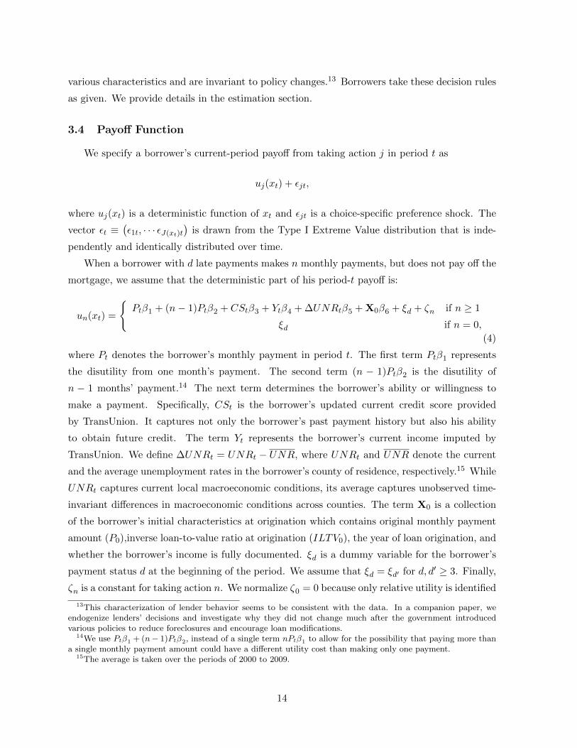
3.4 Payoff Function
We specify a borrower’s current-period payoff from taking action j in period t as
uj(xt) + εjt,
where uj(xt) is a deterministic function of xt and εjt is a choice-specific preference shock. The
vector εt ≡(ε1t, · · · εJ(xt)t
)is drawn from the Type I Extreme Value distribution that is inde-
pendently and identically distributed over time.
When a borrower with d late payments makes n monthly payments, but does not pay off the
mortgage, we assume that the deterministic part of his period-t payoff is:
un(xt) =
{Ptβ1 + (n− 1)Ptβ2 + CStβ3 + Ytβ4 + ∆UNRtβ5 + X0β6 + ξd + ζn if n ≥ 1
ξd if n = 0,
(4)
where Pt denotes the borrower’s monthly payment in period t. The first term Ptβ1 represents
the disutility from one month’s payment. The second term (n − 1)Ptβ2 is the disutility of
n − 1 months’ payment.14 The next term determines the borrower’s ability or willingness to
make a payment. Specifically, CSt is the borrower’s updated current credit score provided
by TransUnion. It captures not only the borrower’s past payment history but also his ability
to obtain future credit. The term Yt represents the borrower’s current income imputed by
TransUnion. We define ∆UNRt = UNRt − UNR, where UNRt and UNR denote the current
and the average unemployment rates in the borrower’s county of residence, respectively.15 While
UNRt captures current local macroeconomic conditions, its average captures unobserved time-
invariant differences in macroeconomic conditions across counties. The term X0 is a collection
of the borrower’s initial characteristics at origination which contains original monthly payment
amount (P0),inverse loan-to-value ratio at origination (ILTV0), the year of loan origination, and
whether the borrower’s income is fully documented. ξd is a dummy variable for the borrower’s
payment status d at the beginning of the period. We assume that ξd = ξd′ for d, d′ ≥ 3. Finally,
ζn is a constant for taking action n. We normalize ζ0 = 0 because only relative utility is identified
13This characterization of lender behavior seems to be consistent with the data. In a companion paper, weendogenize lenders’ decisions and investigate why they did not change much after the government introducedvarious policies to reduce foreclosures and encourage loan modifications.
14We use Ptβ1 + (n− 1)Ptβ2, instead of a single term nPtβ1 to allow for the possibility that paying more thana single monthly payment amount could have a different utility cost than making only one payment.
15The average is taken over the periods of 2000 to 2009.
14
in a discrete choice model.
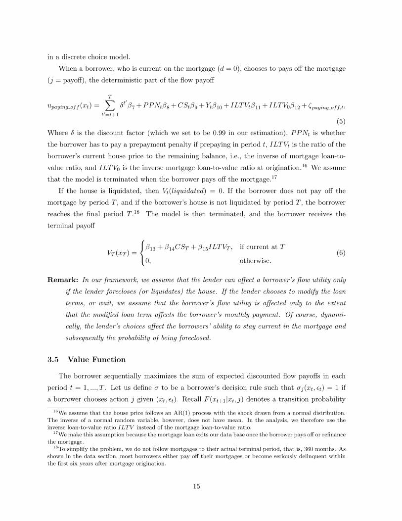
When a borrower, who is current on the mortgage (d = 0), chooses to pays off the mortgage
(j = payoff), the deterministic part of the flow payoff
Where δ is the discount factor (which we set to be 0.99 in our estimation), PPNt is whether
the borrower has to pay a prepayment penalty if prepaying in period t, ILTVt is the ratio of the
borrower’s current house price to the remaining balance, i.e., the inverse of mortgage loan-to-
value ratio, and ILTV0 is the inverse mortgage loan-to-value ratio at origination.16 We assume
that the model is terminated when the borrower pays off the mortgage.17
If the house is liquidated, then Vt(liquidated) = 0. If the borrower does not pay off the
mortgage by period T , and if the borrower’s house is not liquidated by period T , the borrower
reaches the final period T .18 The model is then terminated, and the borrower receives the
terminal payoff
VT (xT ) =
β13 + β14CST + β15ILTVT , if current at T
0, otherwise.(6)
Remark: In our framework, we assume that the lender can affect a borrower’s flow utility only
if the lender forecloses (or liquidates) the house. If the lender chooses to modify the loan
terms, or wait, we assume that the borrower’s flow utility is affected only to the extent
that the modified loan term affects the borrower’s monthly payment. Of course, dynami-
cally, the lender’s choices affect the borrowers’ ability to stay current in the mortgage and
subsequently the probability of being foreclosed.
3.5 Value Function
The borrower sequentially maximizes the sum of expected discounted flow payoffs in each
period t = 1, ..., T . Let us define σ to be a borrower’s decision rule such that σj(xt, εt) = 1 if
a borrower chooses action j given (xt, εt). Recall F (xt+1|xt, j) denotes a transition probability
16We assume that the house price follows an AR(1) process with the shock drawn from a normal distribution.The inverse of a normal random variable, however, does not have mean. In the analysis, we therefore use theinverse loan-to-value ratio ILTV instead of the mortgage loan-to-value ratio.
17We make this assumption because the mortgage loan exits our data base once the borrower pays off or refinancethe mortgage.
18To simplify the problem, we do not follow mortgages to their actual terminal period, that is, 360 months. Asshown in the data section, most borrowers either pay off their mortgages or become seriously delinquent withinthe first six years after mortgage origination.
15
function of state variables which depends on the current state xt and an endogenous choice j.
We can then express the borrower’s problem recursively as follows:
V (xt;σ) = Eεt
∑j∈J(xt)
σj(xt, εt)
{uj(xt) + εjt + δ
∫xt+1∈Xt
V (xt+1;σ)dF (xt+1|xt, j)
} . (7)
The borrower’s optimal decision rule σ∗ is such that V (xt;σ∗b) ≥ V (xt;σ) for any possible decision
rule σ in all xt (t = 1, · · · , T ).
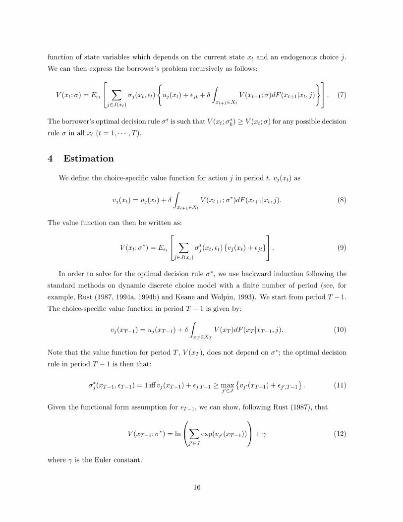
4 Estimation
We define the choice-specific value function for action j in period t, vj(xt) as
vj(xt) = uj(xt) + δ
∫xt+1∈Xt
V (xt+1;σ∗)dF (xt+1|xt, j). (8)
The value function can then be written as:
V (xt;σ∗) = Eεt
∑j∈J(xt)
σ∗j (xt, εt) {vj(xt) + εjt}
. (9)
In order to solve for the optimal decision rule σ∗, we use backward induction following the
standard methods on dynamic discrete choice model with a finite number of period (see, for
example, Rust (1987, 1994a, 1994b) and Keane and Wolpin, 1993). We start from period T − 1.
The choice-specific value function in period T − 1 is given by:
vj(xT−1) = uj(xT−1) + δ
∫xT∈XT
V (xT )dF (xT |xT−1, j). (10)
Note that the value function for period T , V (xT ), does not depend on σ∗; the optimal decision
Given the functional form assumption for εT−1, we can show, following Rust (1987), that
V (xT−1;σ∗) = ln
∑j′∈J
exp(vj′(xT−1))
+ γ (12)
where γ is the Euler constant.
16
Now let us consider the borrower’s optimal decision rule in period T−2. In order to calculate
vj(xT−2), we need to know∫xT−1∈Xt
V (xT−1;σ∗)dF (xT−1|xT−2, j), which can be calculated using
equation (12). We then derive σ∗j (xT−2, εT−2) and V (xT−2;σ∗) similarly as we did in period
T − 1. We repeat this process until we reach the initial period. In general, the borrower’s
optimal decision rule in period t is:
σ∗j (xt, εt) = 1 if vj(xt) + εjt ≥ maxj′∈J
{vj′(xt) + εj′t
}, (13)
and
V (xt;σ∗) = log
∑j′∈J
exp(vj′(xt))
+ γ. (14)
Moreover, a borrower’s conditional choice probability for alternative j ∈ J (xt) is given by:
pj(xt;σ∗) ≡ Eεt [σ∗j (xt, εt)] =
exp(vj(xt))∑j′∈J exp(vj′(xt))
. (15)
We estimate the model using maximum likelihood. In the data, we observe a path of states
and choices for each individual i: (xi,ai) ≡ {(xit,ait)}Tt=1, where ait ≡ {aijt}j∈J(xit), and aijt is
defined to be a dummy variable equals to one when individual i chose action j in period t. The
likelihood of observing (xi,ai) given initial state xi1 and parameter θ for individual i is:
L(xi,ai|xi1; θ) =
T∏t=1
l(ait, xi,t+1|xit; θ), (16)
where l(ait, xi,t+1|xit; θ) is the likelihood of observing (ait, xi,t+1) given state xit and parameter
θ:
l(ait, xi,t+1|xit; θ) =∏
j∈J(xit)
[pj(xt; θ)f(xi,t+1|xit, j)]aijt . (17)
Parameter estimate θ∗ maximizes the log-likelihood for the whole sample, i.e,
θ∗ = arg max lnL(θ) =
I∑i=1
ln (L(xi,ai|xi1; θ))
=I∑i=1
T∑t=1
∑j∈J(xit)
aijt [ln (pj(xt; θ)) + ln f(xi,t+1|xt, j)] .
17
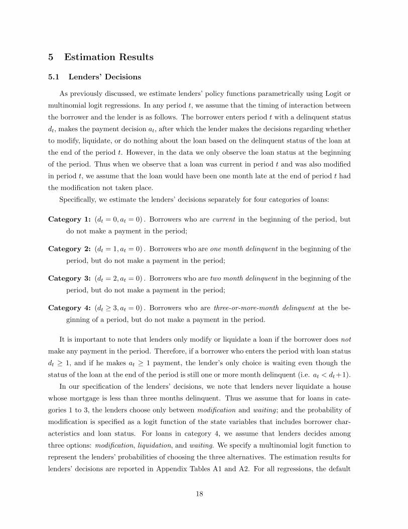
5 Estimation Results
5.1 Lenders’ Decisions
As previously discussed, we estimate lenders’ policy functions parametrically using Logit or
multinomial logit regressions. In any period t, we assume that the timing of interaction between
the borrower and the lender is as follows. The borrower enters period t with a delinquent status
dt, makes the payment decision at, after which the lender makes the decisions regarding whether
to modify, liquidate, or do nothing about the loan based on the delinquent status of the loan at
the end of the period t. However, in the data we only observe the loan status at the beginning
of the period. Thus when we observe that a loan was current in period t and was also modified
in period t, we assume that the loan would have been one month late at the end of period t had
the modification not taken place.
Specifically, we estimate the lenders’ decisions separately for four categories of loans:
Category 1: (dt = 0, at = 0) . Borrowers who are current in the beginning of the period, but
do not make a payment in the period;
Category 2: (dt = 1, at = 0) . Borrowers who are one month delinquent in the beginning of the
period, but do not make a payment in the period;
Category 3: (dt = 2, at = 0) . Borrowers who are two month delinquent in the beginning of the
period, but do not make a payment in the period;
Category 4: (dt ≥ 3, at = 0) . Borrowers who are three-or-more-month delinquent at the be-
ginning of a period, but do not make a payment in the period.
It is important to note that lenders only modify or liquidate a loan if the borrower does not
make any payment in the period. Therefore, if a borrower who enters the period with loan status
dt ≥ 1, and if he makes at ≥ 1 payment, the lender’s only choice is waiting even though the
status of the loan at the end of the period is still one or more month delinquent (i.e. at < dt+1).
In our specification of the lenders’ decisions, we note that lenders never liquidate a house
whose mortgage is less than three months delinquent. Thus we assume that for loans in cate-
gories 1 to 3, the lenders choose only between modification and waiting ; and the probability of
modification is specified as a logit function of the state variables that includes borrower char-
acteristics and loan status. For loans in category 4, we assume that lenders decides among
three options: modification, liquidation, and waiting. We specify a multinomial logit function to
represent the lenders’ probabilities of choosing the three alternatives. The estimation results for
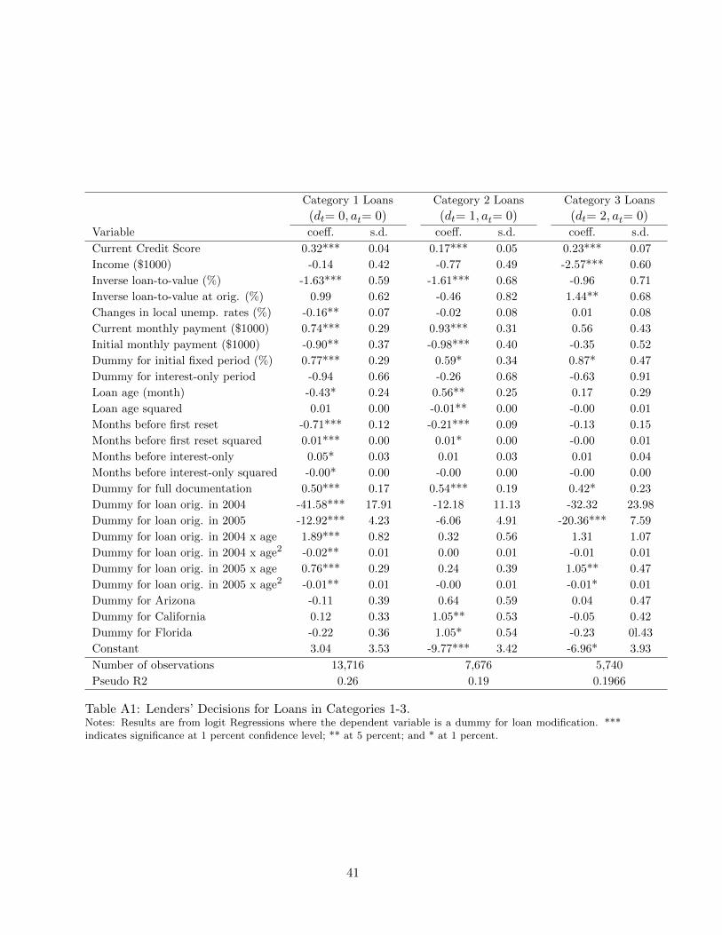
lenders’ decisions are reported in Appendix Tables A1 and A2. For all regressions, the default
18
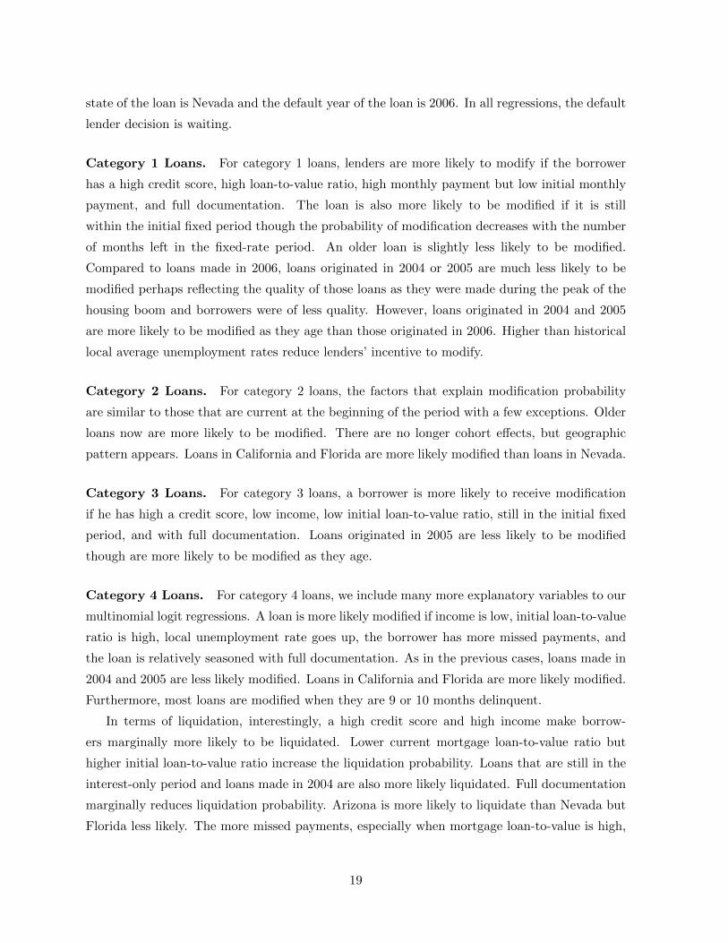
state of the loan is Nevada and the default year of the loan is 2006. In all regressions, the default
lender decision is waiting.
Category 1 Loans. For category 1 loans, lenders are more likely to modify if the borrower
has a high credit score, high loan-to-value ratio, high monthly payment but low initial monthly
payment, and full documentation. The loan is also more likely to be modified if it is still
within the initial fixed period though the probability of modification decreases with the number
of months left in the fixed-rate period. An older loan is slightly less likely to be modified.
Compared to loans made in 2006, loans originated in 2004 or 2005 are much less likely to be
modified perhaps reflecting the quality of those loans as they were made during the peak of the
housing boom and borrowers were of less quality. However, loans originated in 2004 and 2005
are more likely to be modified as they age than those originated in 2006. Higher than historical
local average unemployment rates reduce lenders’ incentive to modify.
Category 2 Loans. For category 2 loans, the factors that explain modification probability
are similar to those that are current at the beginning of the period with a few exceptions. Older
loans now are more likely to be modified. There are no longer cohort effects, but geographic
pattern appears. Loans in California and Florida are more likely modified than loans in Nevada.
Category 3 Loans. For category 3 loans, a borrower is more likely to receive modification
if he has high a credit score, low income, low initial loan-to-value ratio, still in the initial fixed
period, and with full documentation. Loans originated in 2005 are less likely to be modified
though are more likely to be modified as they age.
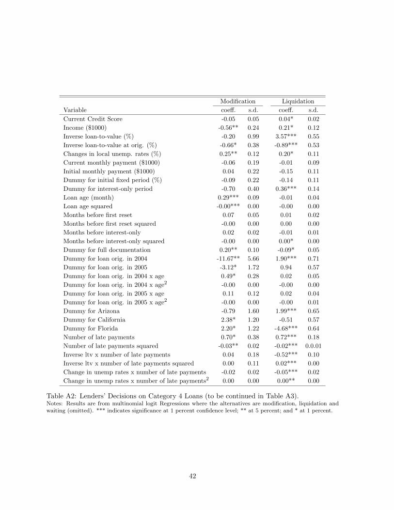
Category 4 Loans. For category 4 loans, we include many more explanatory variables to our
multinomial logit regressions. A loan is more likely modified if income is low, initial loan-to-value
ratio is high, local unemployment rate goes up, the borrower has more missed payments, and
the loan is relatively seasoned with full documentation. As in the previous cases, loans made in
2004 and 2005 are less likely modified. Loans in California and Florida are more likely modified.
Furthermore, most loans are modified when they are 9 or 10 months delinquent.
In terms of liquidation, interestingly, a high credit score and high income make borrow-
ers marginally more likely to be liquidated. Lower current mortgage loan-to-value ratio but
higher initial loan-to-value ratio increase the liquidation probability. Loans that are still in the
interest-only period and loans made in 2004 are also more likely liquidated. Full documentation
marginally reduces liquidation probability. Arizona is more likely to liquidate than Nevada but
Florida less likely. The more missed payments, especially when mortgage loan-to-value is high,
19
the more likely the loan will be liquidated. However, the effect is weaker when local unemploy-
ment rates also go up. Finally, the most liquidation occurs when the loan misses 8 or 9 months
of payment.
Remark. Note that in the data section we documented that the most popular modification is
recapitalization coupled with interest rate reset. After modification, borrowers’ payment
status is brought to current. For simplification, we assume in our analysis that the new
reset interest rate is the initial teaser interest rate during the fixed-interest period of ARM.
We also assume that the modified loan is a fixed rate mortgage with the maturity equal to
the remainder of the initial loan. This simplification allows us to avoid having to estimate
a separate lender decision rule on the new reset interest rate upon modification.19
5.2 Estimates of the Stochastic Processes
In Section 3.2, we also described that borrowers and lenders have beliefs about some stochas-
tic processes such as the evolution of Libor rates, the local housing prices, local unemployment
rates, income and credit scores. We assume that the borrowers have rational expectations about
these processes and estimate them using the ex post realizations of these processes. The es-
timates for these stochastic processes are reported in Table 4. Note that the processes of log
credit score is endogenous for the borrower because its evolution depend on the payment status
on mortgage loans, whose evolution depends on the borrower’s payment decisions.
Table 4 shows that all the variables depend strongly on their lagged values, i.e., they ex-
hibit strong persistence. For credit scores, missing mortgage payments also impact significantly
negatively on their values.
5.3 Borrowers’ Payoff Function Parameters
Table 5 presents the coefficient estimates in the three payoff functions associated with the
three payment decisions. From Panel A, we see that a borrower derives negative utilities from
high mortgage payments, and more so if he makes more than one payment in a given month.
Additionally, he is more likely to make payments when his credit score is high but less likely to
make payments when the local unemployment rate is high as his payment ability is positively
correlated with his credit score but negatively correlated with the local unemployment rate.
Interestingly, the higher the current income, the less likely the borrower will make the mortgage
payment. This counter intuitive result may stem from the imprecise nature of the income
estimate by TransUnion. In terms of conditions at origination, a borrower’s payment ability
19In the data, the mean differnce between the new interest rate upon modification and the initial teaser rate is16 basis points and the median is 37 basis points. Therefore this assumption is a rough approximation.
Dummy for initial fixed period (%) 0.77*** 0.29 0.59* 0.34 0.87* 0.47
Dummy for interest-only period -0.94 0.66 -0.26 0.68 -0.63 0.91
Loan age (month) -0.43* 0.24 0.56** 0.25 0.17 0.29
Loan age squared 0.01 0.00 -0.01** 0.00 -0.00 0.01
Months before first reset -0.71*** 0.12 -0.21*** 0.09 -0.13 0.15
Months before first reset squared 0.01*** 0.00 0.01* 0.00 -0.00 0.01
Months before interest-only 0.05* 0.03 0.01 0.03 0.01 0.04
Months before interest-only squared -0.00* 0.00 -0.00 0.00 -0.00 0.00
Dummy for full documentation 0.50*** 0.17 0.54*** 0.19 0.42* 0.23
Dummy for loan orig. in 2004 -41.58*** 17.91 -12.18 11.13 -32.32 23.98
Dummy for loan orig. in 2005 -12.92*** 4.23 -6.06 4.91 -20.36*** 7.59
Dummy for loan orig. in 2004 x age 1.89*** 0.82 0.32 0.56 1.31 1.07
Dummy for loan orig. in 2004 x age2 -0.02** 0.01 0.00 0.01 -0.01 0.01
Dummy for loan orig. in 2005 x age 0.76*** 0.29 0.24 0.39 1.05** 0.47
Dummy for loan orig. in 2005 x age2 -0.01** 0.01 -0.00 0.01 -0.01* 0.01
Dummy for Arizona -0.11 0.39 0.64 0.59 0.04 0.47
Dummy for California 0.12 0.33 1.05** 0.53 -0.05 0.42
Dummy for Florida -0.22 0.36 1.05* 0.54 -0.23 0l.43
Constant 3.04 3.53 -9.77*** 3.42 -6.96* 3.93
Number of observations 13,716 7,676 5,740
Pseudo R2 0.26 0.19 0.1966
Table A1: Lenders’ Decisions for Loans in Categories 1-3.Notes: Results are from logit Regressions where the dependent variable is a dummy for loan modification. ***indicates significance at 1 percent confidence level; ** at 5 percent; and * at 1 percent.
41
Modification Liquidation
Variable coeff. s.d. coeff. s.d.
Current Credit Score -0.05 0.05 0.04* 0.02
Income ($1000) -0.56** 0.24 0.21* 0.12
Inverse loan-to-value (%) -0.20 0.99 3.57*** 0.55
Inverse loan-to-value at orig. (%) -0.66* 0.38 -0.89*** 0.53
Changes in local unemp. rates (%) 0.25** 0.12 0.20* 0.11
Current monthly payment ($1000) -0.06 0.19 -0.01 0.09
Dummy for initial fixed period (%) -0.09 0.22 -0.14 0.11
Dummy for interest-only period -0.70 0.40 0.36*** 0.14
Loan age (month) 0.29*** 0.09 -0.01 0.04
Loan age squared -0.00*** 0.00 -0.00 0.00
Months before first reset 0.07 0.05 0.01 0.02
Months before first reset squared -0.00 0.00 0.00 0.00
Months before interest-only 0.02 0.02 -0.01 0.01
Months before interest-only squared -0.00 0.00 0.00* 0.00
Dummy for full documentation 0.20** 0.10 -0.09* 0.05
Dummy for loan orig. in 2004 -11.67** 5.66 1.90*** 0.71
Dummy for loan orig. in 2005 -3.12* 1.72 0.94 0.57
Dummy for loan orig. in 2004 x age 0.49* 0.28 0.02 0.05
Dummy for loan orig. in 2004 x age2 -0.00 0.00 -0.00 0.00
Dummy for loan orig. in 2005 x age 0.11 0.12 0.02 0.04
Dummy for loan orig. in 2005 x age2 -0.00 0.00 -0.00 0.01
Dummy for Arizona -0.79 1.60 1.99*** 0.65
Dummy for California 2.38* 1.20 -0.51 0.57
Dummy for Florida 2.20* 1.22 -4.68*** 0.64
Number of late payments 0.70* 0.38 0.72*** 0.18
Number of late payments squared -0.03** 0.02 -0.02*** 0.0.01
Inverse ltv x number of late payments 0.04 0.18 -0.52*** 0.10
Inverse ltv x number of late payments squared 0.00 0.11 0.02*** 0.00
Change in unemp rates x number of late payments -0.02 0.02 -0.05*** 0.02
Change in unemp rates x number of late payments2 0.00 0.00 0.00** 0.00
Table A2: Lenders’ Decisions on Category 4 Loans (to be continued in Table A3).Notes: Results are from multinomial logit Regressions where the alternatives are modification, liquidation andwaiting (omitted). *** indicates significance at 1 percent confidence level; ** at 5 percent; and * at 1 percent.
42
Modification Liquidation
Variable coeff. s.d. coeff. s.d.
Dummy for 4 months deliq. 1.45 0.97 -3.74*** 0.69
Dummy for 5 months deliq. 0.96 0.84 -2.47*** 0.48
Dummy for 6 months deliq. 1.01 0.71 -2.19*** 0.40
Dummy for 7 months deliq. 0.47 0.60 -0.59* 0.32
Dummy for 8 months deliq. 0.54 0.50 0.67*** 0.25
Dummy for 9 months deliq. 0.75* 0.41 0.42** 0.20
Dummy for 10 months deliq. 0.60* 0.35 0.10 0.16
Dummy for 11 months deliq. 0.23 0.32 0.13 0.13
Arizona x months of deliq. 0.00 0.37 -0.20** 0.10
Arizona x months of deliq. squared -0.01 0.02 0.00 0.00
California x months of deliq. -0.46* 0.25 0.13 0.09
California x months of deliq. squared 0.02 0.01 -0.01** 0.00
Florida x months of deliq. -0.50** 0.25 0.48*** 0.10
Florida x months of deliq. squared 0.02 0.01 -0.01*** 0.00
Originated in 2004 x months of deliq. -0.21 0.16 -0.29*** 0.10
Originated in 2004 x months of deliq. squared 0.01 0.01 0.01*** 0.00
Originated in 2005 x months of deliq. -0.07 0.10 -0.19*** 0.07
Originated in 2005 x months of deliq. squared 0.00 0.01 0.01*** 0.00
Constant -10.98*** 2.66 -5.44*** 1.29
Number of observations 33,449
Pseudo R2 0.15
Table A3: Lenders’ Decisions on Category 4 Loans (continued from A2).Notes: Results are from multinomial logit Regressions where the alternatives are modification, liquidation andwaiting (omitted). *** indicates significance at 1 percent confidence level; ** at 5 percent; and * at 1 percent.