The dynamics of chimera states in heterogeneous

Kuramoto networks

Carlo R. Laing a

aInstitute of Information and Mathematical Sciences, Massey University, Private Bag102 904 NSMC, Auckland, New Zealand.

Abstract

We study a variety of mixed synchronous/incoherent (“chimera”) states in sev-eral heterogeneous networks of coupled phase oscillators. For each network, therecently-discovered Ott-Antonsen ansatz is used to reduce the number of variablesin the PDE governing the evolution of the probability density function by one, re-sulting in a time-evolution PDE for a variable with as many spatial dimensions asthe network. Bifurcation analysis is performed on the steady states of these PDEs.The results emphasise the commonality of the dynamics of the different networks,and provide stability information that was previously inferred.

Key words: Kuramoto, phase oscillators, synchrony, non-local, bifurcation.

1 Introduction

The dynamics of coupled oscillator networks has been of great interest formany years, with numerous applications from the biological and physicalworld [1–3]. One of the simplest such networks is the Kuramoto model,where each oscillator is described by a single angular variable (or phase),and the oscillators interact via a trigonometric function of phase differ-ences [4–6]. Recently a number of authors have studied states in networksof identical Kuramoto oscillators for which some oscillators are synchro-nised with one another, while the remainder are incoherent [7–15], referredto by Abrams et al. as “chimera states.” So far, four network topologies havebeen considered:

(1) A ring or line of oscillators with nonlocal coupling [12,7,10,9,11,14].

Email address: c.r.laing@massey.ac.nz (Carlo R. Laing).

Preprint submitted to Elsevier Science 4 May 2009

(2) A two-dimensional array of oscillators with nonlocal coupling [15].(3) An all-to-all coupled network, but with inhomogeneous coupling

strengths [13].(4) Two subnetworks, with all-to-all coupling both within and between

subnetworks [8,12].

The first analysis of such states was performed by Kuramoto and Battog-tokh (KB) [14], who considered a ring of oscillators. These authors definedan order parameter in terms of the states of the oscillators, wrote the dy-namics of the oscillators in terms of this order parameter, and solved for theorder parameter in a self-consistent manner, thus showing that such statesexisted. Abrams et al. [7,10] then analysed the functional equation derivedby KB [14], showed that it was equivalent, in a particular case, to four scalarequations and investigated how solutions of these equations changed as pa-rameters were varied. They found that chimera states bifurcated from stateswith no spatial structure. More recently, Omel’chenko et al. [11] and Sethiaet al. [9] performed a similar analysis to KB [14] but including delays.

Shima and Kuramoto [15] considered a two-dimensional array of phase os-cillators and found spiral waves with “phase-randomised cores.” Most ofthe oscillators (involved in the spiral) were synchronised, having the samefrequency but different phases, while the remainder (at the spiral’s core)were incoherent, with seemingly independent phases. These authors per-formed a similar analysis to KB [14], deriving an equation to be solvedself-consistently and showing that solutions of this equation agreed withsimulations of the full system.

Ko and Ermentrout [13] considered a network of all-to-all coupled oscil-lators, but with coupling strengths chosen from a power-law distribution.They found partially-locked states and analysed them using the self-consis-tency approach of KB [14].

In refs. [13,11,7,10,12] bifurcation diagrams are shown, with stability of so-lutions marked. However, these stabilities all seem to have been inferredrather than calculated. Stable states are found through simulation of thenetwork of oscillators and the corresponding branch of solutions of the self-consistent equation is identified as stable. Turning points on curves of so-lutions are assumed to be saddle-node bifurcations, resulting in unstablebranches of solutions. Abrams et al. [8] were the first to consider the dy-namics of (i.e. stability of) chimera states, analysing a system comprisedof two sub-networks. They used the recent discovery of Ott and Antonsen(OA) [16], that certain networks of phase oscillators have low-dimensionaldynamics, to derive a pair of nonlinear ODEs exactly describing chimerastates in their network. The stability of such solutions and their bifurca-tions were investigated. However, Pikovsky and Rosenblum [17] showed

2

using the approach of Watanabe and Strogatz [18] that the results in [8]were incomplete.

All of the papers [7–11,13–15] considered networks of identical oscillators.In contrast, Laing [12] considered chimera states in networks of noniden-tical oscillators (with intrinsic frequencies chosen from a distribution) andfound that — within limits — chimeras are robust to heterogeneity.Laing [12] also provided evidence to support the observation of Martenset al. [19] and Pikovsky and Rosenblum [17] that the OA ansatz [16] cor-rectly predicts the dynamics of Kuramoto-type networks when the oscilla-tors have randomly-distributed frequencies.

In this paper we use the OA ansatz to derive equations describing the dy-namics of the networks referred to in points 1-3 above, when the networksare heterogeneous, and analyse these equations. This work greatly extendsthat in [12] and demonstrates that all of the networks in points 1-4 abovecan be analysed in the same way.

In Sec. 2 we consider the ring topology of Kuramoto and Battogtokh [14]and others, putting on a solid footing the stability results of Laing [12],showing that Hopf bifurcations can occur in such systems, and that Hopfand saddle-node bifurcations are arranged in parameter space around aTakens-Bogdanov point. In Sec. 3 we consider a network with power-lawdistributed coupling strengths, and recover results similar to those of Koand Ermentrout [13]. In Sec. 4 we consider spiral waves in two spatial di-mensions, deriving a number of new results. Two models similar to thatstudied in Sec. 2 are investigated in Sec. 5, and we reproduce some resultsof others, although using a different approach. We conclude in Sec. 6.

2 A ring of oscillators

Consider a ring of N phase oscillators with nonlocal coupling [12,7,10,14].For this network a chimera state refers to a statistically-stationary state forwhich oscillators on part of the ring are synchronised while those on therest of the ring are incoherent. See Fig. 1 for an example.

3

0 100 200 300 400 5000

1

2

3

4

5

6

Index

φ

Fig. 1. A snapshot of a chimera solution of the system (1). N = 500, β = 0.2 and theωi are taken from a Dirac delta distribution. G(x) = (1 + 0.95 cos x)/(2π).

2.1 Analysis

The system is

dφidt

= ωi −2π

N

N∑

j=1

G

(2π|i− j|

N

)cos (φi − φj − β) (1)

for i = 1, . . .N , where φi is an angular variable and the natural frequenciesωi are chosen from a distribution g(ω). The coupling function G is periodicwith period 2π.

We move to the continuum limit (N → ∞) and assume there is a probabil-ity density function f(x, ω, φ, t) characterising the state of the system. Thisfunction satisfies the continuity equation [8,6]

∂f

∂t+

∂

∂φ(fv) = 0 (2)

where

v = ω −∫ 2π

0G(x− y)

∫ ∞

−∞

∫ π

−πcos [φ− φ′ − β]f(y, ω, φ′, t)dφ′dωdy (3)

4

and φ = φ(x) and φ′ = φ(y). Defining the order parameter

R(x, t) ≡∫ 2π

0G(x− y)

∫ ∞

−∞

∫ π

−πe−iφ

′

f(y, ω, φ′, t)dφ′ dω dy (4)

we can rewrite

v = ω −1

2

[Rei(φ−β) +Re−i(φ−β)

](5)

where an overbar indicates complex conjugate. Following Ott and Anton-sen [16], we write

f(x, ω, φ, t) =g(ω)

2π

[1 +

∞∑

n=1

hn(x, ω, t)einφ + c.c.

](6)

where “c.c.” indicates the complex conjugate of the previous term, and as-sume that hn(x, ω, t) = [a(x, ω, t)]n, i.e. that the nth coefficient is a function,[a(x, ω, t)], raised to the nth power. Substituting (6) into (2) we obtain

∂a

∂t= −iωa+ (i/2)

[Re−iβ + Reiβa2

](7)

where

R(x, t) =∫ π

−πG(x− y)

∫ ∞

−∞g(ω)a(y, ω, t) dω dy (8)

This ansatz, which effectively replaces the infinite set of functions, hn bya single function, a, is non-trivial, and its validity is discussed in Sec. 6.

In this paper we will always assume that the ω are chosen from a Lorentziandistribution with half-width-at-half-maximum D, i.e.

g(ω) =D/π

(ω − ω0)2 +D2=

1

2πi

(1

ω − ω0 − iD−

1

ω − ω0 + iD

)(9)

where ω0 is the centre of the distribution. For non-delayed, autonomoussystems we can always set ω0 = 0 without loss of generality, by movingto a rotating coordinate frame. With g(ω) from (9) and ω0 = 0 we can usecontour integration to perform the integral over ω in (8), obtaining [12,16]

R(x, t) =∫ π

−πG(x− y)a(y,−iD, t) dy (10)

Writing z(x, t) = a(x,−iD, t) we have

∂z

∂t= −Dz + (i/2)

[Re−iβ + Reiβ z2

](11)

where

R(x, t) =∫ π

−πG(x− y)z(y, t) dy (12)

5

As is known [7,12,14], the analysis of (11)-(12) is simplified by moving to arotating coordinate frame (rotating in the φ direction, not x). Thus we definez ≡ zeiΩt, where Ω is as yet unknown. We find that z satisfies

∂z

∂t= (iΩ −D)z + (i/2)

[Re−iβ + Reiβz2

](13)

where

R(x, t) =∫ π

−πG(x− y)z(y, t) dy (14)

As other authors have done [7,10,12] we assume thatG(x) = (1+A cosx)/(2π),and that z is even in x. Then, henceforth dropping the hat on R, we have

R(x, t) = z0(t) + z1(t) cosx (15)

where

z0(t) =1

2π

∫ 2π

0z(x, t) dx and z1(t) =

A

2π

∫ 2π

0z(x, t) cos (x) dx (16)

We are interested in stationary solutions of (13)-(14), their stability and thebifurcations they undergo as parameters are varied. A stationary solutionof (13) is a function z(x) which satisfies

(iΩ −D)z + (i/2)[Re−iβ +Reiβz2

]= 0 (17)

where R is also independent of time. Note that for any solution z of (17),zeiψ , where ψ is arbitrary, is also a solution of (17). We can compare thesestationary solutions with those already found using a self-consistency ar-gument [12,7]. Solving (17) for z we obtain

z =D − iΩ ±

√(D − iΩ)2 + |R|2

iReiβ(18)

Choosing the negative square root and taking the spatial average of (18) weobtain

z0 =1

2π

∫ 2π

0

D − iΩ −√

(D − iΩ)2 + |R(x)|2

iR(x)eiβdx (19)

which (up to the allowable arbitrary rotation of z in the complex plane [7])is the same as equation (28) in [12]. Similarly, multiplying both sides of (18)by A cosx and integrating we obtain

z1 =A

2π

∫ 2π

0

D − iΩ −

√(D − iΩ)2 + |R(x)|2

iR(x)eiβ

cos (x) dx (20)

which (after the same arbitrary rotation mentioned above) is the same asequation (29) in [12]. The self-consistency argument of others [12,7,10] con-sists of simultaneously solving (19)-(20) for the scalars z0, z1 and Ω. This

6

self-consistency argument shows that chimera states exist, but does not giveany information about the dynamics and stability of such solutions.

Now consider the physical interpretation of solutions of (17). Consideringstationary states in the coordinate frame rotating with angular velocity Ωand fixing ω = −iD, we see that the probability density function F (φ) atposition x has proportionality

F (φ) ∼∞∑

n=−∞

[z(x)]neinφ (21)

Note that for this series to converge we must have |z| ≤ 1. Now if z = re−iθ,where 0 ≤ r < 1, we have

F (φ) =1 − r2

2π[1 − 2r cos (φ− θ) + r2], (22)

the Poisson kernel, whereas if r = 1 we have

F (φ) = δ(φ− θ), (23)

the Dirac delta function. Thus θ gives the value of φ at which the maximumof F occurs, and r is a measure of the “peakedness” of the distribution;r = 0 corresponds to a uniform distribution, while r = 1 corresponds to theDirac delta. This physical interpretation also shows why solutions of (17)are invariant under the rigid rotation z 7→ zeiψ mentioned above — it isjust a manifestation of the invariance of the full system (1) under the shiftφi 7→ φi + ψ ∀i.

2.2 Results

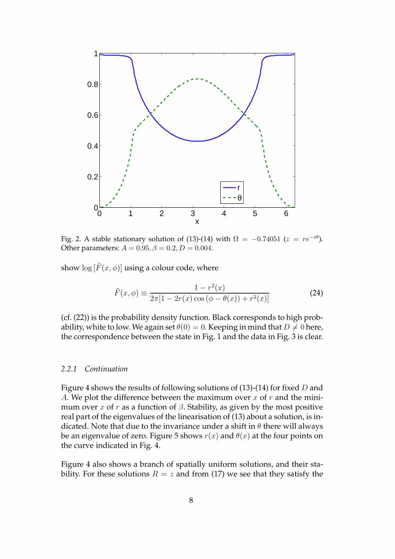
We now discuss numerical solutions of (13)-(14). To find them, the domainis discretised into 500 evenly-spaced points and the corresponding ODEsare then solved. A typical solution is shown in Fig. 2, where we write z =re−iθ. Note that θ(x) is only specified up to a shift, so we set θ(0) = 0. Re-call that values of r close to 1 (at both ends of the domain) correspond totightly synchronised oscillators, while lower values of r (in the centre of thedomain) correspond to less coherent oscillators. While the correspondencewith the state in Fig. 1 is not exact, due to the non-zero value of D usedhere, the general features are the same.

Figure 3 shows another representation of the solution in Fig. 2. Here we

7

0 1 2 3 4 5 60

0.2

0.4

0.6

0.8

1

x

rθ

Fig. 2. A stable stationary solution of (13)-(14) with Ω = −0.74051 (z = re−iθ).Other parameters: A = 0.95, β = 0.2,D = 0.004.

show log [F (x, φ)] using a colour code, where

F (x, φ) ≡1 − r2(x)

2π[1 − 2r(x) cos (φ− θ(x)) + r2(x)](24)

(cf. (22)) is the probability density function. Black corresponds to high prob-ability, white to low. We again set θ(0) = 0. Keeping in mind thatD 6= 0 here,the correspondence between the state in Fig. 1 and the data in Fig. 3 is clear.

2.2.1 Continuation

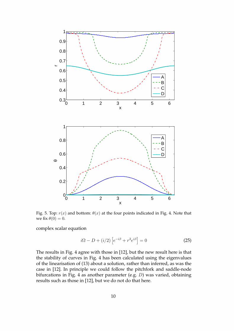
Figure 4 shows the results of following solutions of (13)-(14) for fixedD andA. We plot the difference between the maximum over x of r and the mini-mum over x of r as a function of β. Stability, as given by the most positivereal part of the eigenvalues of the linearisation of (13) about a solution, is in-dicated. Note that due to the invariance under a shift in θ there will alwaysbe an eigenvalue of zero. Figure 5 shows r(x) and θ(x) at the four points onthe curve indicated in Fig. 4.

Figure 4 also shows a branch of spatially uniform solutions, and their sta-bility. For these solutions R = z and from (17) we see that they satisfy the

8

x

φ

0 1 2 3 4 5 6−3

−2

−1

0

1

2

3

Fig. 3. Another representation of the solution shown in Fig. 2. Black correspondsto high probability, white to low. See text for more details.

0 0.05 0.1 0.15 0.2 0.25

0

0.1

0.2

0.3

0.4

0.5

0.6

β

max

(r)−

min

(r)

A

B

C

D

Fig. 4. max (r)−min (r) as a function of β for stationary solutions of (13)-(14). Solidline: stable; dashed line: unstable. r(x) and θ(x) at the four points indicated areplotted in Fig. 5. Parameters are D = 0.004, A = 0.95.

9

0 1 2 3 4 5 60.3

0.4

0.5

0.6

0.7

0.8

0.9

1

x

r

0 1 2 3 4 5 60

0.2

0.4

0.6

0.8

1

x

θ

ABCD

ABCD

Fig. 5. Top: r(x) and bottom: θ(x) at the four points indicated in Fig. 4. Note thatwe fix θ(0) = 0.

complex scalar equation

iΩ −D + (i/2)[e−iβ + r2eiβ

]= 0 (25)

The results in Fig. 4 agree with those in [12], but the new result here is thatthe stability of curves in Fig. 4 has been calculated using the eigenvaluesof the linearisation of (13) about a solution, rather than inferred, as was thecase in [12]. In principle we could follow the pitchfork and saddle-nodebifurcations in Fig. 4 as another parameter (e.g. D) was varied, obtainingresults such as those in [12], but we do not do that here.

10

Time

x

200 400 600 800 1000

0

2

4

6

0.4

0.6

0.8

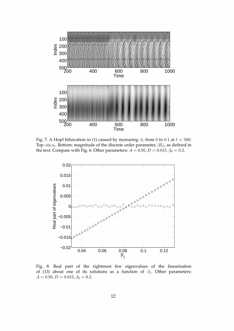
Fig. 6. A Hopf bifurcation in (13)-(14) caused by increasing β1 from 0 to 0.1 att = 500. The colour encodes r. Other parameters: A = 0.95,D = 0.015, β0 = 0.2.

2.2.2 Hopf bifurcations

One of the questions posed in [8] was: do breathing (i.e. oscillating) chimerasexist in one-dimensional arrays of oscillators such as the one studied in thissection? Here we answer this question in the affirmative by introducing pa-rameter heterogeneity, letting β(x) = β0 − β1 cos (x) in (13)-(14). Figure 6shows an apparent Hopf bifurcation as β1 is abruptly increased from zero.To verify that this bifurcation also occurs in the network of oscillators, (1),we performed the same change in parameters and the results are shown inFig. 7. The top panel shows sin (φi) as a function of time and the bottompanel shows |Ri| as a function of time, where Ri is the spatially-discreteversion of R(x, t), defined using (4) as

Rk(t) =2π

N

N∑

j=1

G

(2π|k − j|

N

)e−iφj (26)

The onset of oscillations in the discrete network is clear.

Figure 8 shows the real part of the rightmost few eigenvalues of the lin-earisation of (13) about a solution similar to the initial condition shownin Fig. 6, as a function of β1. The crossing of the imaginary axis by a pairof complex conjugate eigenvalues as β1 increases through approximately0.085 is clear. (The imaginary part of these eigenvalues, not shown, variesbetween approximately 0.13i and 0.15i over the parameter range shown.)The zero eigenvalue mentioned above is also evident.

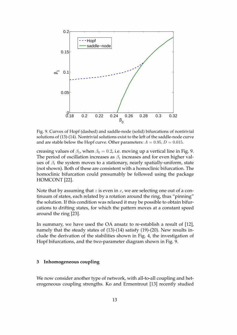
In Fig. 9 we show the curves of Hopf bifurcations in the (β0, β1) plane.Also shown is the continuation of the saddle-node bifurcation that occurswhen β1 = 0 (see Fig. 4). These curves meet at a Takens-Bogdanov (double-zero eigenvalue) bifurcation. Generically, one expects a curve of homoclinicbifurcations to emanate from a Takens-Bogdanov point [20,21]. Figure 10shows evidence that such a curve does exist in this case, lying above thecurve of Hopf bifurcations, just as in Fig. 4 of [8]. In Fig. 10 we show r(π)(i.e. in the middle of the domain) as a function of time for successively in-

11

Time

Inde

x

200 400 600 800 1000

100

200

300

400

500

Time

Inde

x

200 400 600 800 1000

100

200

300

400

500

Fig. 7. A Hopf bifurcation in (1) caused by increasing β1 from 0 to 0.1 at t = 500.Top: sin φi. Bottom: magnitude of the discrete order parameter, |Ri|, as defined inthe text. Compare with Fig. 6. Other parameters: A = 0.95,D = 0.015, β0 = 0.2.

0.04 0.06 0.08 0.1 0.12−0.02

−0.015

−0.01

−0.005

0

0.005

0.01

0.015

0.02

β1

Rea

l par

t of e

igen

valu

es

Fig. 8. Real part of the rightmost few eigenvalues of the linearisationof (13) about one of its solutions as a function of β1. Other parameters:A = 0.95,D = 0.015, β0 = 0.2.

12

0.18 0.2 0.22 0.24 0.26 0.28 0.3 0.320

0.05

0.1

0.15

0.2

β0

β 1

Hopfsaddle−node

Fig. 9. Curves of Hopf (dashed) and saddle-node (solid) bifurcations of nontrivialsolutions of (13)-(14). Nontrivial solutions exist to the left of the saddle-node curveand are stable below the Hopf curve. Other parameters: A = 0.95,D = 0.015.

creasing values of β1, when β0 = 0.2, i.e. moving up a vertical line in Fig. 9.The period of oscillation increases as β1 increases and for even higher val-ues of β1 the system moves to a stationary, nearly spatially-uniform, state(not shown). Both of these are consistent with a homoclinic bifurcation. Thehomoclinic bifurcation could presumably be followed using the packageHOMCONT [22].

Note that by assuming that z is even in x, we are selecting one out of a con-tinuum of states, each related by a rotation around the ring, thus “pinning”the solution. If this condition was relaxed it may be possible to obtain bifur-cations to drifting states, for which the pattern moves at a constant speedaround the ring [23].

In summary, we have used the OA ansatz to re-establish a result of [12],namely that the steady states of (13)-(14) satisfy (19)-(20). New results in-clude the derivation of the stabilities shown in Fig. 4, the investigation ofHopf bifurcations, and the two-parameter diagram shown in Fig. 9.

3 Inhomogeneous coupling

We now consider another type of network, with all-to-all coupling and het-erogeneous coupling strengths. Ko and Ermentrout [13] recently studied

13

1000 1100 1200 1300 1400 15000

0.5

1C

Time

1000 1100 1200 1300 1400 15000

0.5

1B

1000 1100 1200 1300 1400 15000

0.5

1A

Fig. 10. A plot of r(π) as a function of time for (A): β1 = 0.09, (B): β1 = 0.1, (C):β1 = 0.1125. Other parameters: A = 0.95,D = 0.015, β0 = 0.2.

the following model

dφidt

= ωi +Ki

N

N∑

j=1

H(φj − φi) (27)

where H(φ) = sin (φ− β) + sin β and the Ki are taken from a truncatedpower-law distribution Γ(K), where

Γ(K) =

CK−γ for K ∈ [Kmin, Kmax]

0 otherwise(28)

and C is a normalising factor such that∫∞0 Γ(K)dK = 1. As before, let the ωi

be chosen from the probability density function g(ω). These authors foundthat for certain ranges of parameters (and identical ωi) partial locking, inwhich some fraction of the oscillators synchronise, occurs. An example ofsuch partial locking is shown in Fig. 11, where we have ordered the os-cillators by their K value. We see that it is oscillators with low K whichsynchronise, oscillators with higher K have higher average frequency, andthat the synchronous oscillators do not rotate with the intrinsic frequencyof the oscillators, ωi, which are all zero in this case.

14

0 100 200 300 400 5000

2

4

6

Ki

Tim

e

100 200 300 400 5000

50

100

150

200

0 100 200 300 400 5000

2

4

6

Index

φ i

Fig. 11. Top: Ki versus oscillator index. Middle: sinφi (colour–coded) over a time interval of length 200. Bottom: a snapshot ofthe phases φi. Transients have been removed. Other parameters:N = 500,Kmin = 0.1,Kmax = 5, γ = 1.5, β = 0.4π, ωi = 0 ∀i.

3.1 Analysis

We now analyse the continuum limit of (27). The analysis is analogous tothat in Sec. 2.1, but the variable x is now replaced by K. First rewrite (27) as

dφidt

= ωi +Ki sin β +Ki

N

N∑

j=1

sin(φj − φi − β) (29)

15

In the continuum limit, we again assume the existence of a probability den-sity function f(K,ω, φ, t) which satisfies the continuity equation

∂f

∂t+

∂

∂φ(fv) = 0 (30)

where

v = ω +K sin β +K∫ ∞

0Γ(K)

∫ ∞

−∞

∫ 2π

0sin [φ′ − φ− β]f(K,ω, φ′, t)dφ′ dω dK

(31)Defining the (scalar) order parameter

R(t) =∫ ∞

0Γ(K)

∫ ∞

−∞

∫ 2π

0eiφ

′

f(K,ω, φ′, t)dφ′ dω dK (32)

we can write

v = ω +K sin β +K

2i

[Re−i(φ+β) − Rei(φ+β)

](33)

As before, we use the OA ansatz to write

f(K,ω, φ, t) =g(ω)

2π

[1 +

∞∑

n=1

[a(K,ω, t)]neinφ + c.c.

](34)

and substitute this into (30) and (32) to obtain

∂a

∂t= −i(ω +K sin β)a+ (K/2)

[Reiβ − Re−iβa2

](35)

where

R(t) =∫ ∞

0Γ(K)

∫ ∞

−∞g(ω)a(K,ω, t) dω dK (36)

If

g(ω) =D/π

ω2 +D2(37)

then

R(t) =∫ ∞

0Γ(K)a(K,−iD, t) dK (38)

Writing z(K, t) = a(K,−iD, t) we have

∂z

∂t= −(D + iK sin β)z + (K/2)

[Reiβ − Re−iβ z2

](39)

where

R(t) =∫ ∞

0Γ(K)z(K, t) dK (40)

Moving to a rotating coordinate frame: z ≡ zeiΩt we see that z satisfies

∂z

∂t= −(D + i[K sin β − Ω])z + (K/2)

[Reiβ − Re−iβz2

](41)

16

where

R(t) =∫ ∞

0Γ(K)z(K, t) dK (42)

Let us now compare our results with those of Ko and Ermentrout [13], de-rived using the self-consistency arguments of Kuramoto [14,7]. Ko and Er-mentrout used identical oscillators, so set D = 0. Then, dropping the hat on

R, steady states of (41) satisfy

KRe−iβz2 + 2i[K sin β − Ω]z −KReiβ = 0 (43)

Solving for z and taking the positive square root we obtain

z =−i[K sin β − Ω] +

√K2|R|2 − (K sin β − Ω)2

KRe−iβ(44)

At stationarity the phase of R is arbitrary so we can assume that R is real.Using (42) we obtain

R2 = e−iβ∫ ∞

0Γ(K)

i[K sin β − Ω] +

√K2R2 − (K sin β − Ω)2

K

dK (45)

which, after writing ∆ = −Ω, is eqn. (17) in [13]. We note that z = 0 isalways a solution of (41)-(42).

3.2 Results

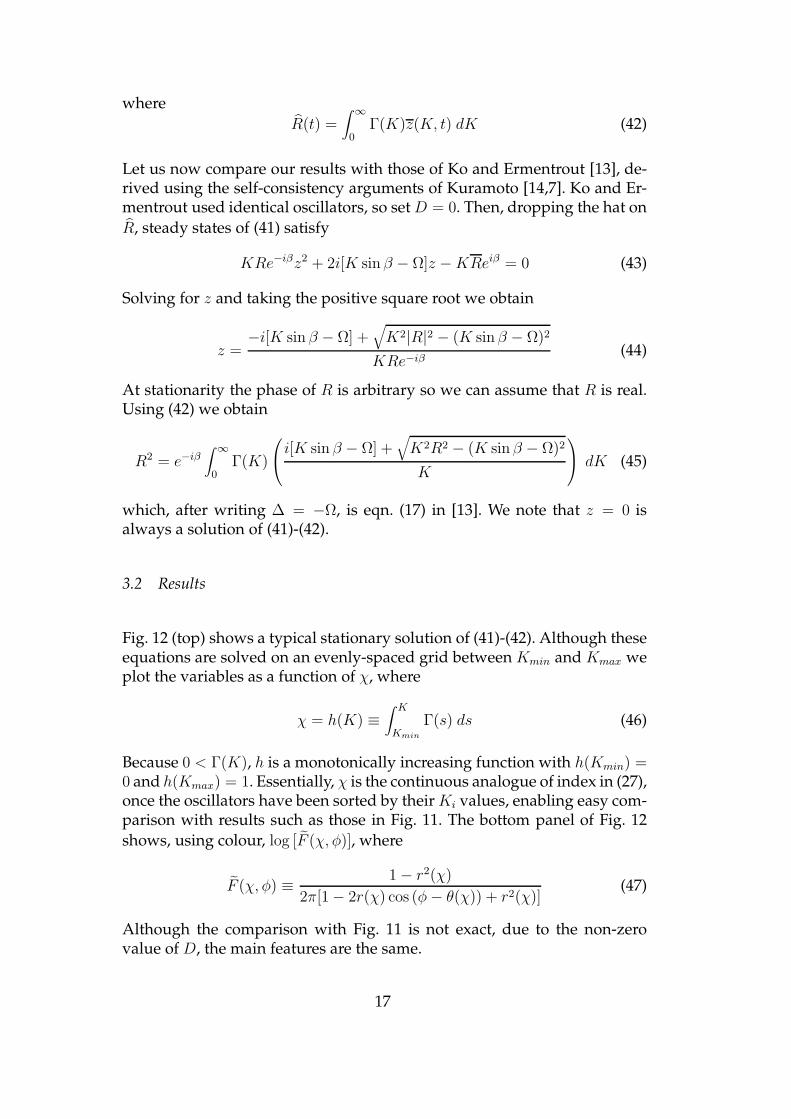
Fig. 12 (top) shows a typical stationary solution of (41)-(42). Although theseequations are solved on an evenly-spaced grid between Kmin and Kmax weplot the variables as a function of χ, where

χ = h(K) ≡∫ K

Kmin

Γ(s) ds (46)

Because 0 < Γ(K), h is a monotonically increasing function with h(Kmin) =0 and h(Kmax) = 1. Essentially, χ is the continuous analogue of index in (27),once the oscillators have been sorted by their Ki values, enabling easy com-parison with results such as those in Fig. 11. The bottom panel of Fig. 12

shows, using colour, log [F (χ, φ)], where

F (χ, φ) ≡1 − r2(χ)

2π[1 − 2r(χ) cos (φ− θ(χ)) + r2(χ)](47)

Although the comparison with Fig. 11 is not exact, due to the non-zerovalue of D, the main features are the same.

17

0 0.2 0.4 0.6 0.8 10

0.2

0.4

0.6

0.8

1

1.2

1.4

χ

rθ

χ

φ

0 0.2 0.4 0.6 0.8 1−3

−2

−1

0

1

2

3

Fig. 12. Top: A stable stationary solution of (41)-(42) with Ω = 0.069031

(z = re−iθ). We have set θ(0) = 0. Bottom: log [F (χ, φ)] (47) in-dicated with a colour code (black high, white low). Other parameters:Kmin = 0.1,Kmax = 5, γ = 1.5, β = 0.4π,D = 0.0001.

Figure 13 shows the result of continuing solutions of (41)-(42) as β is varied,for two different values of D, with stability indicated. The upper (lower)stable curves in the upper (lower) panel correspond to the solutions foundby [13], while the other stable branches with |R| ≈ 1 correspond to thein phase synchronous states found by them. (Note that these authors usedidentical oscillators, i.e. D = 0). The branches terminate for large β at pitch-fork bifurcations involving the z = 0 (i.e. completely incoherent) state thatis always a solution. This state is stable for β larger than the values at which

18

0.25 0.3 0.35 0.4 0.45 0.50

0.02

0.04

0.06

0.08

Ω

A

B

C

0.25 0.3 0.35 0.4 0.45 0.50

0.2

0.4

0.6

0.8

1

β/π

|R|

Fig. 13. Curves of stationary solutions of (41)-(42) for D = 0.01 (leftmost curves)and D = 0.003 (rightmost curves). Top: Ω and bottom: |R| as a function of β. Solidline: stable, dashed line: unstable. Solutions at the points marked are shown inFig. 14.

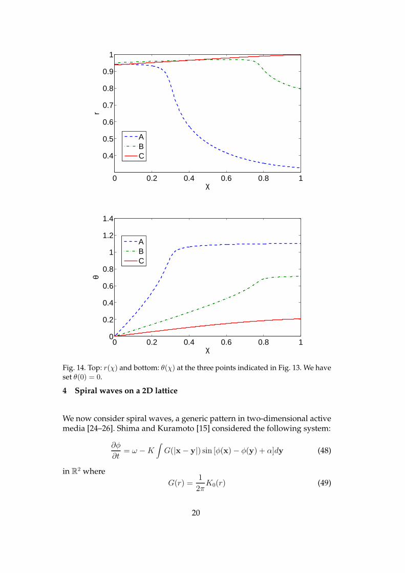
the curves in Fig. 13 terminate. This bifurcation diagram has been verifiedby simulating the original network (27) (not shown). Figure 14 shows r(χ)and θ(χ) at the three points indicated in Fig. 13.

All of the results in this section are new, although Ko and Ermentrout [13]derived (45) using the self-consistency argument of Kuramoto and Battog-tokh [14].

19

0 0.2 0.4 0.6 0.8 1

0.4

0.5

0.6

0.7

0.8

0.9

1

χ

r

ABC

0 0.2 0.4 0.6 0.8 10

0.2

0.4

0.6

0.8

1

1.2

1.4

χ

θ

ABC

Fig. 14. Top: r(χ) and bottom: θ(χ) at the three points indicated in Fig. 13. We haveset θ(0) = 0.

4 Spiral waves on a 2D lattice

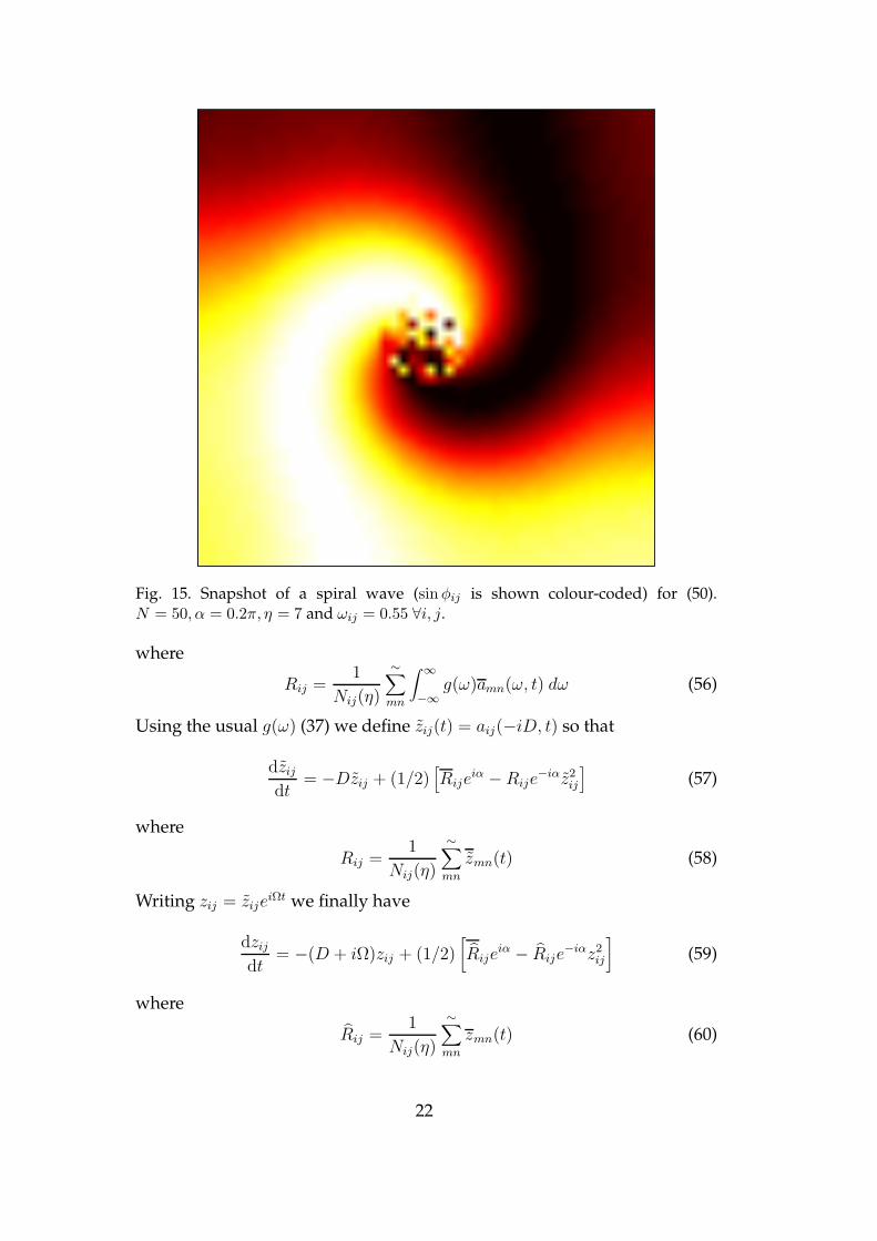
We now consider spiral waves, a generic pattern in two-dimensional activemedia [24–26]. Shima and Kuramoto [15] considered the following system:

∂φ

∂t= ω −K

∫G(|x − y|) sin [φ(x) − φ(y) + α]dy (48)

in R2 where

G(r) =1

2πK0(r) (49)

20

andK0 is the modified Bessel function of the second kind. They found spiralwaves with “phase-randomised cores,” and showed their existence usingthe self-consistency argument of Kuramoto [14]. Kim et al. [27] also foundspiral waves with phase-randomised cores in two-dimensional arrays ofcoupled phase oscillators, and it is their system that we study here. Theequations are

dφijdt

= ωij +1

Nij(η)

∼∑

mn

sin (φmn − φij − α) (50)

for 1 ≤ i ≤ N, 1 ≤ j ≤ N , where (i, j) indicates the position on the lat-tice and

∑∼mn indicates a sum over all lattice points within a distance η of

the point (i, j); there are Nij(η) of these. Note that we do not use periodicboundary conditions, soNij(η) will be smaller for points near the boundarythan for points well away from the boundary. A snapshot of a typical spiralfor η = 7 is shown in Fig. 15. The unsynchronised oscillators at the spiralcore are clearly visible.

While spiral waves in systems with local interactions have been studied bya number of authors [24,25,28], their behaviour in systems with non-localinteractions, as is the case here, is much less well-studied [29].

4.1 Analysis

We do not move to a spatial continuum, but as usual assume the existence ofa probability density function fij(ω, φ, t) which satisfies the usual continuityequation (2), where

v = ωij +1

Nij(η)

∼∑

mn

∫ ∞

−∞

∫ π

−πsin (φmn − φij − α)fmn(ω, φmn, t) dφmn dω (51)

Defining the order parameter

Rij =1

Nij(η)

∼∑

mn

∫ ∞

−∞

∫ π

−πeiφmnfmn(ω, φmn, t) dφmn dω (52)

we see that

v = ωij +1

2i

[Rije

−i(φij+α) − Rijei(φij+α)

](53)

Writing

fij(ω, φ, t) =g(ω)

2π

[1 +

∞∑

n=1

[aij(ω, t)]neinφ + c.c.

](54)

we find that

daijdt

= −iωijaij + (1/2)[Rije

iα − Rije−iαa2

ij

](55)

21

Fig. 15. Snapshot of a spiral wave (sin φij is shown colour-coded) for (50).N = 50, α = 0.2π, η = 7 and ωij = 0.55 ∀i, j.

where

Rij =1

Nij(η)

∼∑

mn

∫ ∞

−∞g(ω)amn(ω, t) dω (56)

Using the usual g(ω) (37) we define zij(t) = aij(−iD, t) so that

dzijdt

= −Dzij + (1/2)[Rije

iα −Rije−iαz2

ij

](57)

where

Rij =1

Nij(η)

∼∑

mn

zmn(t) (58)

Writing zij = zijeiΩt we finally have

dzijdt

= −(D + iΩ)zij + (1/2)[Rije

iα − Rije−iαz2

ij

](59)

where

Rij =1

Nij(η)

∼∑

mn

zmn(t) (60)

22

0

0.2

0.4

0.6

0.8

1

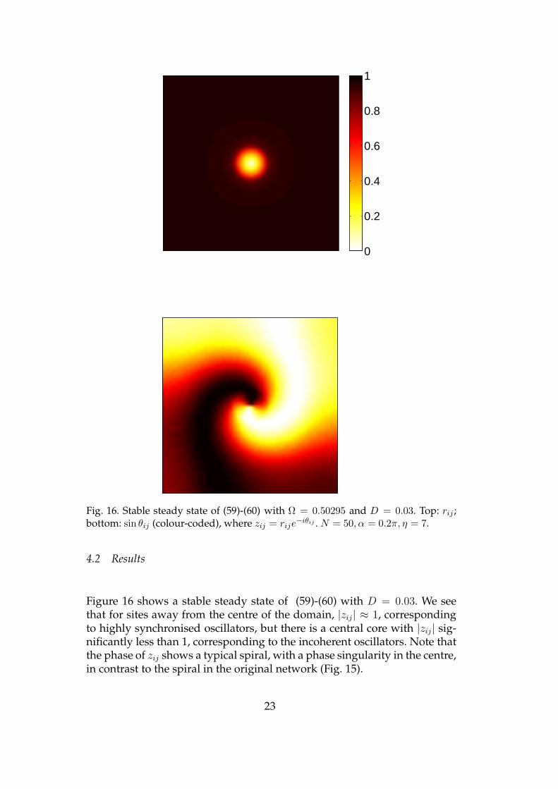
Fig. 16. Stable steady state of (59)-(60) with Ω = 0.50295 and D = 0.03. Top: rij ;bottom: sin θij (colour-coded), where zij = rije

−iθij . N = 50, α = 0.2π, η = 7.

4.2 Results

Figure 16 shows a stable steady state of (59)-(60) with D = 0.03. We seethat for sites away from the centre of the domain, |zij| ≈ 1, correspondingto highly synchronised oscillators, but there is a central core with |zij| sig-nificantly less than 1, corresponding to the incoherent oscillators. Note thatthe phase of zij shows a typical spiral, with a phase singularity in the centre,in contrast to the spiral in the original network (Fig. 15).

23

0 0.1 0.2 0.3 0.40

0.1

0.2

0.3

0.4

0.5

0.6

α/pi

Ω

C

B

A

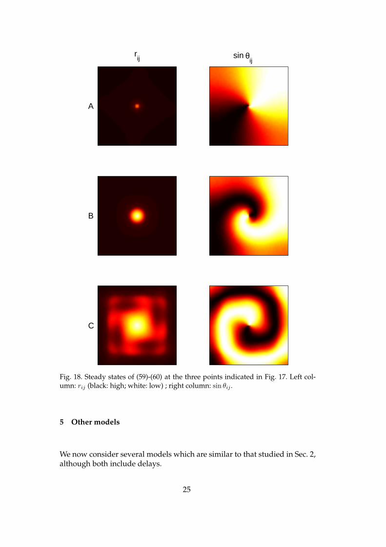
Fig. 17. Steady states of (59)-(60) with D = 0.03. Solid line: stable; dashed line:unstable. Solutions at the points marked are shown in Fig. 18.

4.2.1 Varying parameters

Varying α we obtain the family of spiral waves shown in Fig. 17. Severalrepresentative solutions are shown in Fig. 18. We see that as α is decreased,the width of the incoherent core decreases. (This was verified by simula-tions of (50), not shown.) Note that the square domain has a significant in-fluence on the solution for large α, and further investigations of this systemshould probably use a circular domain [29,25].

4.2.2 Hopf bifurcation

We can also cause Hopf bifurcations in (59)-(60) by making α spatially-dependent, as in Sec. 2.2.2. We set αij = α0 + α1Φij , where

Φij = exp(−5

[(2i− 51)/49]2 + [(2j − 51)/49]2

)(61)

i.e. Φij is a Gaussian, centred at the centre of the domain (recall thatN = 50).In Fig. 19 we have plotted r along a horizontal slice through the centre ofthe domain, and show the effect of abruptly switching α1 from 0 to 0.05π.The “spot” of low r simultaneously moves away from and starts to rotateabout the centre of the domain, and the dynamics are analogous to thoseresulting from a Hopf bifurcation of a normal spiral wave [26,29]. Detect-ing and following the Hopf bifurcation, as in Sec. 2.2.2, should be possible,although time-consuming. The presence of this Hopf bifurcation was alsoverified in the original network (50) (not shown).

All of the results in the section, obtained using the OA ansatz, are new.

24

θsinij

rij

A

B

C

Fig. 18. Steady states of (59)-(60) at the three points indicated in Fig. 17. Left col-umn: rij (black: high; white: low) ; right column: sin θij .

5 Other models

We now consider several models which are similar to that studied in Sec. 2,although both include delays.

25

Time

j

1000 1500 2000

20

40 0.20.40.60.8

Fig. 19. r25j when α1 is switched from 0 to 0.05π at t = 1000. D = 0.02, α0 = 0.2π.

5.1 Omel’chenko et al.

Omel’chenko et al. [11] studied the model

∂φ

∂t= ω−

C

2

∫ 1

−1sin [φ(x, t) − φ(y, t)] dy−

Kρ(x)

2

∫ 1

−1sin [φ(x, t) − φ(y, t− τ)] dy

(62)where

ρ(x) =ae−a|x|

1 − e−a(63)

and 0 < a.

5.1.1 Analysis

Define a density function f(x, ω, φ, t) which satisfies (2) where

v=ω −C

2

∫ 1

−1

∫ ∞

−∞

∫ π

−πsin [φ(t) − φ′(t)]f(y, ω, φ′, t) dφ′ dω dy

−Kρ(x)

2

∫ 1

−1

∫ ∞

−∞

∫ π

−πsin [φ(t) − φ′(t− τ)] f(y, ω, φ′, t) dφ′ dω dy (64)

where φ = φ(x) and φ′ = φ(y). Defining the (spatially-independent) orderparameter

R(t) =1

2

∫ 1

−1

∫ ∞

−∞

∫ π

−πeiφ

′(t)f(y, ω, φ′, t)dφ′ dω dy (65)

we can rewrite

v = ω −C

2i

[R(t)eiφ −R(t)e−iφ

]−Kρ(x)

2i

[R(t− τ)eiφ − R(t− τ)e−iφ

](66)

Writing

f(x, ω, φ, t) =g(ω)

2π

[1 +

∞∑

n=1

[a(x, ω, t)]neinφ + c.c.

](67)

26

we find that a satisfies

∂a

∂t= −iωa+

1

2

[CR(t) +Kρ(x)R(t− τ) − a2 CR(t) +Kρ(x)R(t− τ)

]

(68)where

R(t) =1

2

∫ 1

−1

∫ ∞

−∞g(ω)a(y, ω, t) dω dy (69)

Because we are considering a delay system we can no longer assume with-out loss of generality that the mean of g(ω) is zero. We use g(ω) given by (9),and defining z(x, t) = a(x, ω0 − iD, t) we obtain

∂z

∂t= −(iω0+D)z+

1

2

[CR(t) +Kρ(x)R(t− τ) − z2 CR(t) +Kρ(x)R(t − τ)

]

(70)where

R(t) =1

2

∫ 1

−1

¯z(t) dy (71)

and letting z = zeiΩt we obtain

∂z

∂t=−(D + i[ω0 − Ω])z

+1

2

[CR(t) +Kρ(x)R(t− τ)eiΩτ

− z2CR(t) +Kρ(x)R(t− τ)e−iΩτ

](72)

where

R(t) =1

2

∫ 1

−1z(t) dy (73)

5.1.2 Results

Fig. 20 shows snapshots of solutions of the spatially-discretised versionof (62) for two different values of τ , found using the Matlab routine dde23.Other parameters, as used by [11], are a = 1, C = 0.1π,K = π, ω = ω0 = 2π.In Fig. 21 we show stable stationary solutions of (72)-(73) for the same pa-rameter values as in Fig. 20, for D = 0. We see excellent agreement betweenthe results for a finite network and those from the analysis of the corre-sponding PDE.

27

−1 0 1−1

0

1

x

φ/π

−1 0 1−1

0

1

x

φ/π

Fig. 20. Snapshots of solutions of the spatially-discretised version of (62) for τ = 0.3(left) and τ = 0.6 (right). Compare with Fig. 1 in[11]. 101 oscillators are used. Seetext for other parameters.

−1 0 1

0.4

0.6

0.8

1

x

r

−1 0 1−1

0

1

x

θ/π

−1 0 1

0.4

0.6

0.8

1

x

r

−1 0 1−1

0

1

x

θ/π

Fig. 21. Stable stationary solutions of (72)-(73) for τ = 0.3,Ω = 4.0565 (left) andτ = 0.6,Ω = 8.4981 (right) and D = 0. Same parameters as in Fig. 20. We have setθ(0) = 0 to match the results in Fig. 20.

5.2 Sethia et al.

Sethia et al. [9] studied the model

∂φ

∂t= ω −

∫ L

−LG(x− y) sin [φ(x, t) − φ(y, t− |x− y|/V ) + α] dy (74)

on a ring of circumference 2L, where

G(x) =ke−k|x|

2(1 − e−kL)(75)

28

and V can be thought of as the speed of propagation of signals around thering.

5.2.1 Analysis

Defining a density function f(x, ω, φ, t) results in the usual continuity equa-tion (2) where

v = ω−∫ L

−LG(x−y)

∫ ∞

−∞

∫ π

−πsin [φ(t) − φ′(t− |x− y|/V ) + α]f(y, ω, φ′, t)dφ′dωdy

where φ = φ(x) and φ′ = φ(y). Defining the order parameter

R(x, t) ≡∫ L

−LG(x− y)

∫ ∞

−∞

∫ π

−πeiφ

′(t−|x−y|/V )f(y, ω, φ′, t)dφ′ dω dy (76)

we have

v(φ, t) = ω −1

2i

[Rei(φ+α) − Re−i(φ+α)

]

Writing

f(x, ω, φ, t) =g(ω)

2π

[1 +

∞∑

n=1

[a(x, ω, t)]neinφ + c.c.

](77)

we find∂a

∂t= −iωa+

1

2

[Reiα − Re−iαa2

](78)

where

R(x, t) =∫ L

−LG(x− y)

∫ ∞

−∞g(ω)a(y, ω, t− |x− y|/V ) dω dy (79)

Using g(ω) from (9) and defining z(x, t) = a(x, ω0 − iD, t) we obtain

∂z

∂t= −(iω0 +D)z +

1

2

[Reiα − Re−iαz2

](80)

where

R(x, t) =∫ L

−LG(x− y)z(y, t− |x− y|/V ) dy (81)

and letting z = zeiΩt we have

∂z

∂t= −(D + i[ω0 − Ω])z +

1

2

[Reiα − Re−iαz2

](82)

where

R(x, t) =∫ L

−LG(x− y)z(y, t− |x− y|/V )e−iΩ|x−y|/V dy (83)

In the usual way, steady states of (82) when D = 0 are the same as thosefound using the self-consistency argument, see eqn. (6) in [9].

29

Tim

e

−0.5 0 0.5

35

40

45

50

−0.5 0 0.50

2

4

6

x

φ

Fig. 22. A solution of the spatially-discretised version of (74). Top: sin φ(colour-coded) over a time interval of length 20. Bottom: a snapshot of theφ. We have discretised with 256 spatial points and other parameters areω = 1.1, α = 0.9, V = 1/10.24, k = 4, L = 1/2.

5.2.2 Results

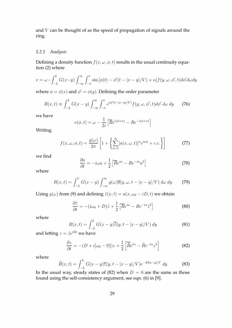
In Fig. 22 we show a typical solution of the spatially-discretised versionof (74), using the same parameters as [9]. We see four coherent regions (thedomain is periodic in x), adjacent ones of which are out of phase, separatedby regions of incoherence.

In Fig. 23 we show a stationary solution of (82)-(83) for D = 0 and the sameother parameters as in Fig. 22. The correspondence with Fig. 22 is excellent.As noted by [9], the solution shown in Fig. 23 is only stable in the space ofspatially-even functions. If this symmetry is not preserved, (82)-(83) havestable travelling wave solutions, for which r is constant and θ is a linearlyincreasing function of space and time (not shown).

6 Discussion

In this paper we have considered a number of infinite networks of cou-pled heterogeneous phase oscillators. For each network we used the OAansatz [16] to derive a PDE, the solutions of which describe the dynamicsof the network. Of course, for each network a more general such PDE exists:the continuity equation (2). However, the power of the OA ansatz is that it

30

−0.5 0 0.50

2

4

6

x

θ

−0.5 0 0.50

0.5

1

r

Fig. 23. A stationary solution of (82)-(83) for D = 0 and Ω = 0.90869.Top: r(x); bottom: θ(x) (z = re−iθ). Other parameters areω = 1.1, α = 0.9, V = 1/10.24, k = 4, L = 1/2.

reduces by one the number of variables in the PDE that needs to be stud-ied. For example, for the model considered in Sec 2, eqn. (2) is a PDE for f ,which is a function of four variables, x, ω, φ and t. The OA ansatz removesthe dependence on φ and we obtain the PDE (7) for a function of only threevariables. The dependence on ω can be integrated out by choosing g(ω) tobe, for example, a Lorentzian or Dirac delta function, and we obtain (13), aPDE for z(x, t). Similarly in Sec. 3 we obtain the PDE (41) for the variable z,which is a function of only K (a space-like variable) and t, and in Sec. 4 weobtain the spatially-indexed ODEs (59).

Effectively, we have greatly generalised the results of Marvel and Strogatz [30],who showed that any system of N identical oscillators governed by the dy-namics

dφjdt

= µe−iφj + λ+ µeiφj (84)

could be solved using the OA ansatz: assume a density

ρ(φ, t) =1

2π

[1 +

∞∑

n=1

α(t)eiφ

n+ c.c

](85)

Then α satisfies the ODE

dα

dt= −i(λα + µ+ µα2) (86)

Marvel and Strogatz stated that the OA ansatz requires identical oscillators

31

and that f and g be independent of the oscillator index. In fact, we haveshown here that we can relax both of these assumptions and still use theOA ansatz, but the price we pay is that we now have a PDE (or N ODEs).For example, in Sec. 2 we find the velocity of each oscillator is given by (5):

v = ω −[Rei(φ−β) + Re−i(φ−β)

]/2 (87)

which is of the form (84), with λ = ω and µ = −Reiβ/2. Here, R is a functionof space (or oscillator index, in the discrete case) and we obtain the PDE (7)

∂a

∂t= −iωa+ (i/2)

[Re−iβ + Reiβa2

](88)

where a is now a function of space too. Similarly, in Sec. 3 we obtain (33)

v = ω +K sin β +K

2i

[Re−i(φ+β) − Rei(φ+β)

](89)

where R is the same for each oscillator. However, K is different for each os-cillator (or K is a continuous variable, in the continuum limit) so we obtainthe PDE (35):

∂a

∂t= −i(ω +K sin β)a+ (K/2)[Reiβ − Re−iβa2] (90)

where a is a function of K as well as t.

We have only considered solutions of the PDEs derived in this paper whenD (the width of the distribution from which intrinsic frequencies are drawn)is not zero (though see Figs. 21 and 23 for exceptions). The correctness of us-ing the OA ansatz to describe stable states of the networks studied here hasbeen the subject of recent discussion [17,30,19,31]. For example, Pikovskyand Rosenblum [17] recently demonstrated using the Watanabe-Strogatz(WS) ansatz [18] that the OA ansatz did not completely describe all of thedynamics possible in the network studied by Abrams et al. [8]. However,there is mounting numerical evidence that the OA ansatz does in fact de-scribe all attracting (and, presumably, hyperbolic) states, if the oscillatorsin the network are non-identical [12,31,16,17,19]. The recent preprint by Ottand Antonsen [32] seems to put these observations on a sound theoreticalbasis. To correctly study the networks considered in this paper when theoscillators are identical it may be necessary to generalise the WS ansatz tothese topologies [33], or it may be that the dynamics really are described byequations such as (13), (41), (59), (72) and (82) withD = 0. We leave the con-nection between the WS and OA ansatze, and the analysis of the equationsjust mentioned when D = 0 for future work.

Regarding the dependence of the results on the specific form of g(ω): otherdistributions with similar pole structures in the complex plane could be

32

used, resulting in similar (although more complicated) equations [12,16].Numerical results with other distributions (e.g. Gaussian) suggest that thereis nothing special about the Lorentzian distribution [12,19,31].

In summary, our main result is the demonstration that a number of differ-ent networks, each capable of supporting “chimera” (and other) states, canbe analysed using the same framework. We have discovered new types ofbehaviour, and put on a solid footing the stability results inferred by oth-ers [13,11,7,10,12]. The results presented here are by no means complete;further analysis of the PDEs derived should result in the discovery of moreinteresting behaviour of coupled oscillator networks.

Acknowledgements

I thank the referees for their useful comments, and for bringing the pre-print [32] to my attention.

References

[1] S. Strogatz. Sync: The Emerging Science of Spontaneous Order. Hyperion, 2003.

[2] A. Pikovsky, M. Rosenblum, and J. Kurths. Synchronization. CambridgeUniversity Press, 2001.

[3] A.T. Winfree. The Geometry of Biological Time. Springer, 2001.

[4] J.A. Acebron, LL Bonilla, C.J. Perez Vicente, F. Ritort, and R. Spigler. TheKuramoto model: A simple paradigm for synchronization phenomena. Rev.Mod. Phys., 77:137–185, 2005.

[5] Yoshiki. Kuramoto. Chemical oscillations, waves, and turbulence. Springer-Verlag,1984.

[6] S.H. Strogatz. From Kuramoto to Crawford: exploring the onset ofsynchronization in populations of coupled oscillators. Physica D, 143:1–20,2000.

[7] Daniel M. Abrams and Steven H. Strogatz. Chimera states in a ring ofnonlocally coupled oscillators. Int. J. Bifn. Chaos, 16:21–37, 2006.

[8] Daniel M. Abrams, Rennie Mirollo, Steven H. Strogatz, and Daniel A. Wiley.Solvable model for chimera states of coupled oscillators. Phys. Rev. Lett.,101:084103, 2008.

[9] G.C. Sethia, A. Sen, and F.M. Atay. Clustered Chimera States in Delay-CoupledOscillator Systems. Phys. Rev. Lett., 100:144102, 2008.

33

[10] Daniel M. Abrams and Steven H. Strogatz. Chimera states for coupledoscillators. Phys. Rev. Lett., 93:174102, 2004.

[11] O.E. Omel’chenko, Y.L. Maistrenko, and P.A. Tass. Chimera States: TheNatural Link Between Coherence and Incoherence. Phys. Rev. Lett., 100:044105,2008.

[12] Carlo R. Laing. Chimera states in heterogeneous networks. Chaos, 19:013113,2009.

[13] T.W. Ko and G.B. Ermentrout. Partially locked states in coupled oscillatorsdue to inhomogeneous coupling. Physical Review E, 78(1):016203, 2008.

[14] Y. Kuramoto and D. Battogtokh. Coexistence of Coherence and Incoherence inNonlocally Coupled Phase Oscillators. Nonlinear Phenom. Complex Syst., 5:380–385, 2002.

[15] S. Shima and Y. Kuramoto. Rotating spiral waves with phase-randomized corein nonlocally coupled oscillators. Physical Review E, 69(3):036213, 2004.

[16] Edward Ott and Thomas M. Antonsen. Low dimensional behavior of largesystems of globally coupled oscillators. Chaos, 18:037113, 2008.

[17] Arkady Pikovsky and Michael Rosenblum. Partially integrable dynamics ofhierarchical populations of coupled oscillators. Phys. Rev. Lett., 101:264103,2008.

[18] S. Watanabe and SH Strogatz. Constants of motion for superconductingJosephson arrays. Physica. D, 74:197–253, 1994.

[19] E. A. Martens, E. Barreto, S. H. Strogatz, E. Ott, P. So, and T. M. Antonsen.Exact results for the kuramoto model with a bimodal frequency distribution.Physical Review E, 79:026204, 2009.

[20] J. Guckenheimer and P. Holmes. Nonlinear Oscillations, Dynamical Systems, andBifurcations of Vector Fields. Springer, 1983.

[21] Y.A. Kuznetsov. Elements of Applied Bifurcation Theory. Springer, 2004.

[22] E. Doedel, RC Paffenroth, AR Champneys, TF Fairgrieve, Y.A. Kuznetsov,B. Sandstede, and X. Wang. AUTO 2000: Continuation and BifurcationSoftware for Ordinary Differential Equations (with HomCont). ConcordiaUniversity, Canada, ftp. cs. concordia. ca/pub/doedel/auto.

[23] C. Laing and S. Coombes. The importance of different timings of excitatoryand inhibitory pathways in neural field models. Network: Computation inNeural Systems, 17(2):151–172, 2006.

[24] M. Bar, A.K. Bangia, and I.G. Kevrekidis. Bifurcation and stability analysis ofrotating chemical spirals in circular domains: Boundary-induced meanderingand stabilization. Physical Review E, 67(5):056126, 2003.

[25] D. Barkley. Linear stability analysis of rotating spiral waves in excitable media.Physical Review Letters, 68(13):2090–2093, 1992.

34

[26] D. Barkley. Euclidean symmetry and the dynamics of rotating spiral waves.Physical Review Letters, 72(1):164–167, 1994.

[27] P.J. Kim, T.W. Ko, H. Jeong, and H.T. Moon. Pattern formation in a two-dimensional array of oscillators with phase-shifted coupling. Physical ReviewE, 70(6):065201, 2004.

[28] G. Bordyugov and H. Engel. Continuation of spiral waves. Physica D:Nonlinear Phenomena, 228(1):49–58, 2007.

[29] C.R. Laing. Spiral waves in nonlocal equations. SIAM Journal on AppliedDynamical Systems, 4(3):588–606, 2005.

[30] Seth A. Marvel and Steven H. Strogatz. Invariant submanifold for series arraysof josephson junctions. Chaos: An Interdisciplinary Journal of Nonlinear Science,19(1):013132, 2009.

[31] L.M. Childs and S.H. Strogatz. Stability diagram for the forced Kuramotomodel. Chaos: An Interdisciplinary Journal of Nonlinear Science, 18:043128, 2008.

[32] Edward Ott and Thomas M. Antonsen. Long Time Evolution of PhaseOscillator Systems. Arxiv preprint arXiv:0902.2773v1, 2009.

[33] Seth A. Marvel, Renato E. Mirollo, and Steven H. Strogatz. Sinusoidallycoupled phase oscillators evolve by Mobius group action. Arxiv preprint,arXiv:0904.1680v1, 2009.

35