THE ECONOMIC CONTRIBUTION OF THE EQUIPMENT LEASING ... · The Economic Contribution of The...

The Economic Contribution of The Equipment Leasing Industry To the U.S. Economy. - 1 -

THE ECONOMIC CONTRIBUTION OF THE EQUIPMENT LEASING INDUSTRY

TO THE U.S. ECONOMY

Prepared for:

EQUIPMENT LEASING ASSOCIATION

PREPARED BY:

Global Insight, Advisory Services Group

610.490.2749

March 1, 2004


Contents

EXECUTIVE SUMMARY .....................................................................................................3

RESULTS..............................................................................................................................3 IMPLICATIONS......................................................................................................................3

INTRODUCTION ...................................................................................................................4

BACKGROUND AND PURPOSE...............................................................................................4

INDUSTRY BACKGROUND AND ECONOMIC TRENDS .............................................4

APPROACH AND METHODOLOGY .................................................................................5

A BRIEF OVERVIEW TO THE STUDY PROCESS ......................................................................5 ECONOMIC CONTRIBUTION ANALYSIS – A FORMAL DESCRIPTION.......................................6

STUDY RESULTS...................................................................................................................9

OVERVIEW...........................................................................................................................9 FULL ADJUSTMENT SCENARIO...........................................................................................10

Overall Economic Contribution – Macroeconomic Indicators...................................10 Composition of Equipment Investment........................................................................10 Employment Impacts – the Effect on Incomes and Employment By Industry .............10

RESTRICTED ADJUSTMENT SCENARIO................................................................................11 Overall Economic Contribution – Macroeconomic Indicators...................................11 Composition of Equipment Investment........................................................................11 Employment Impacts – the Effect on Incomes and Employment By Industry .............11

CONCLUSIONS ....................................................................................................................12

TABLES AND GRAPHS ......................................................................................................14

APPENDIX A: FULL ADJUSTMENT SCENARIO RESULTS......................................17

APPENDIX B: RESTRICTED ADJUSTMENT SCENARIO RESULTS, TOTAL IMPACT..........................................................................................................................................19

APPENDIX C: RESTRICTED ADJUSTMENT SCENARIO RESULTS, DIRECT AND INDIRECT EFFECTS...................................................................................................21

APPENDIX C: RESTRICTED ADJUSTMENT SCENARIO RESULTS, DIRECT AND INDIRECT EFFECTS...................................................................................................21

APPENDIX D: EQUIPMENT INVESTMENT BY INDUSTRY .....................................23

APPENDIX E: OVERVIEW OF THE GLOBAL INSIGHT MACROECONOMIC MODEL..........................................................................................................................................25

APPENDIX F: OVERVIEW OF THE GLOBAL INSIGHT INDUSTRY MODEL INDUSTRIAL ANALYSIS SERVICE MODEL OVERVIEW.................................35


Executive Summary The Equipment Leasing Association (ELA) requested that Global Insight undertake a study to measure the value and contribution of the equipment leasing industry on the U.S. economy. Utilizing its state-of-the-art macroeconomic and industry models, Global Insight was able to evaluate the economic contribution to the U.S. economy.

Results

Key results of the study show that, over the 1997-2002 period, the equipment leasing industry

• Produced between $100 billion and $300 billion additional real GDP. • Produced between $227 billion and $229 billion additional real equipment investment. • Created between 3 million and 5 million additional jobs.

The economic value extends beyond jobs because the incomes of labor and business proprietors are affected as well. Global Insight estimated that the higher level of sustainable jobs attributable to the leasing industry accounts for roughly $375 billion of real personal income annually, of which $255 billion is concentrated in the leasing industry and all related supplier industries. An additional $120 billion accrues to the rest of the economy through additional spending on goods and services in markets that are peripheral to equipment markets.

Implications

Our study implies that the most important contribution of the equipment leasing industry lies in providing access to capital. When leasing is unavailable, the demand for equipment is curtailed, which impacts other industries everywhere along the equipment supply chain. Why this fundamental contribution is so critical, and why its value to the economy is so large, is due to several factors:

• Leasing, as a way of acquiring the use of equipment, cuts across goods-producing and services-producing industries in the U.S. economy.

• Leasing is a crucial approach to acquiring a variety of equipment types, especially high-technology equipment, which is so vital to innovation and growth.

• Leasing arrangements are used by all sizes of businesses, even though their capital requirements may differ.

Several subsidiary benefits extend to the economy. Greater access to capital permits greater entry into markets than might occur without leasing. Markets are potentially more competitive by expanding the pool of market participants. Increasing the market for capital goods at the margin facilitates greater growth in new capital goods production and investment.


Introduction Background and Purpose

One of the major components of U.S. GDP—equipment investment—has undergone a change during the last few decades. Capital equipment for use in the production process by businesses is being increasingly leased, rather than purchased. According to U.S. Department of Census statistics, the rental and leasing services market has grown by roughly 40%: from $76 billion in 1997 to $106 billion in 2000. The market has been experiencing negative or slow growth due to the current economic slowdown.

The Equipment Leasing Association (ELA) requested that Global Insight undertake a study to measure the economic value and contribution of the equipment leasing industry to the U.S. economy. Some of the specific issues of interest include:

• Equipment acquired by U.S. companies via leasing. • Comparison of equipment purchased versus equipment leased. • Contribution to the deployment of technology. • Contribution to productivity changes. • Contribution to the U.S. economy • Contribution to U.S. industrial sectors • Impact on U.S. employment

The purpose and use of this study is to develop public policy assessments, provide better business education, and guide investment decisions. The results will be integrated with strategic planning.

Industry Background and Economic Trends The equipment leasing industry is a fragmented and diverse group of companies, including nearly all the Fortune 100 financial institutions offering a variety of equipment leasing programs and services. The companies include:

• Bank-related organizations. • Manufacturer captive financials. • Independents. • Diversified financial service organizations.

These companies operate in basically four markets: the Micro Ticket Market, consisting of transactions under $25,000; the Small Ticket Market, for transactions of $25,000 to $250,000; the Middle Market, including transactions ranging from $250,000 to $5 million; and the Large Ticket Market, consisting of transactions that exceed $5 million.

Many types of equipment are leased throughout the U.S. economy, including office equipment, IT equipment, manufacturing machinery, transportation equipment, and medical equipment. Many sectors of the U.S. economy lease equipment, including construction, manufacturing, services, and wholesale/retail trade, which exhibit a higher propensity to lease relative to other industrial sectors.


The economic climate since early 2001 has not been a healthy one for capital investment generally. Fortunes in the equipment leasing industry have mirrored the economy, for large and capital spending in particular. Evidence from the industry suggests that the Large Ticket and Middle Market segments were especially affected.1 The large ticket segment saw a decline of roughly 6% in 2002 over the previous year, while volume in the middle market segment declined by over 9% during the same period.

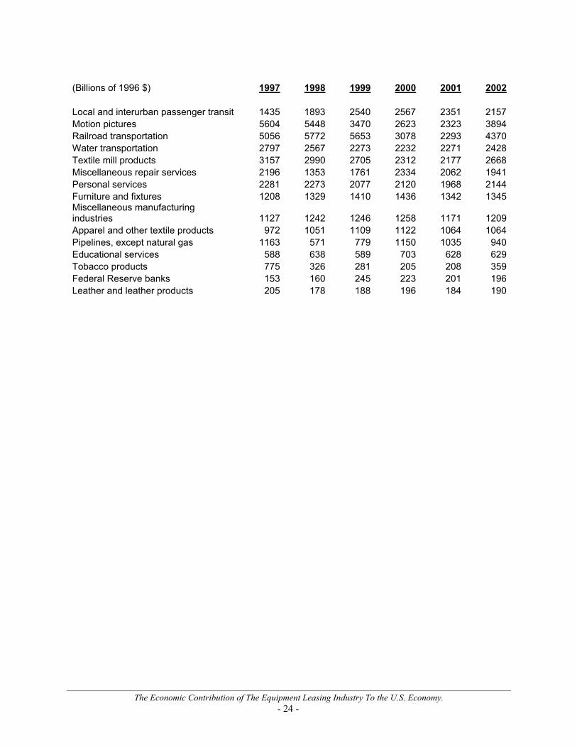
Looking across sectors, we find that there is ample investment volume and growth, as well as decline. Table 1 (Appendix – Tables) exhibits a rank ordering of the top ten industries by the absolute size of equipment investment, where size is measured by the five-year average investment levels. What this short ranking shows is that large volumes of equipment investment are spread across goods-producing and services-producing sectors of the U.S. economy.2

A similar view results when the topline is peeled back to look at equipment leasing by equipment type. Table 2 (Appendix – Tables) shows a very similar pattern of mixed growth results across equipment types.3 For example, while the last five years have not been rewarding in communications equipment leasing, leasing in computer equipment and software has shown positive growth. Recent trends and new information suggest that these industries are well poised for growth in the coming year and beyond.4

Approach and Methodology A Brief Overview to the Study Process

To estimate the economic impact of an industry as important as the equipment leasing industry would be daunting if not for the organized experimental design using the modeling power available. The study required a very controlled plan, which is described in its essence in the following text.

A five-year historical period was chosen as a sufficient period that would allow all of the dynamic effects in the economy to stabilize. The most recent, complete five-year period (1997-2002) was desirable because of the relative freshness of the data. Using that period, the historical data provided a benchmark, or baseline, against which the simulation results could be compared.

The study then created a fiction: if equipment leasing were removed from the U.S. economy, what would be the totality of the impact on the economy at large and on specific indicators of interest. In essence, then, the study measures the value of equipment leasing by asking how much the economy would lose—in the way of real output, real capital investment, and jobs—in its absence.

The study basically required that all equipment be purchased; no leasing option was available. At this stage, it is possible to isolate only the narrow, direct impact of removing the industry itself by comparing key indicators to the historical baseline.

1 Equipment Leasing and Finance Foundation, 2003 State of the Industry Report, sponsored by SAP. 2 A complete listing of equipment investment by industry is shown in Appendix D of this report. Global Insight has provided historical data and projections of (a) final sales by industry and (b) equipment investment by category to the Equipment Leasing Association. 3 Source: Equipment Leasing Association. 4 Global Insight, Inc., U.S. Economic Review, January 2004. See also the Wendover-Global Insight IT Spending Index, http://www.globalinsight.com/Highlight/HighlightDetail742.htm.


However, the magnitude of the impact extends far beyond the leasing industry because the impact resonates throughout the entire chain of equipment buyers and sellers. When leasing is unavailable, demand for equipment is curtailed, and the impact is felt everywhere along the equipment supply chain. This broader aspect of the study permits quantifying the totality of the importance of leasing to goods and services industries.

The study was able to capture a final but important residual effect that added to the final total impact. When a change of this magnitude is made in the economy, there are spillover effects beyond the direct industry impact and the attendant interindustry effects on goods-producing industries and service industries. The additional spending loss (or increase) affects industries on the periphery of those affected by leasing either directly or indirectly. Therefore, by fictionally removing leasing from the economy, the residual effects on the rest of the economy can also be measured.

These are the general steps in developing the analysis. Global Insight developed two separate scenarios, however, in order to frame the possible outcomes. In one scenario, the study restricts the degree to which labor is rehired into the economy. Because of this fairly dramatic absence of response, the economic effects are dramatic as well. The second scenario permits a full and rapid adjustment by industries in reabsorbing labor into the economy. As this occurs, income and output grow faster than in the more restrictive alternative, and consequently, the economic loss is somewhat more muted.

The study essentially provides a range of estimates against which the contribution of the equipment leasing industry can be measured.

Economic Contribution Analysis – A Formal Description

The economic impact of equipment leasing activity can be traced through all U.S. industrial sectors, as well as the macro economy. In this section, we will define the key terms and the conceptual framework that underlie the approach. The terms are:

• Direct impacts – the primary economic impacts caused by changes to the narrowly defined equipment leasing industry, including those directly involved in the leasing process.

• Indirect impacts – the secondary economic impacts caused by changes to broadly defined sectors of the economy, including industries that buy or sell to the equipment leasing industry.

• Induced impacts – the tertiary economic impacts caused by expenditure-induced changes to the economy at large.

The primary objective of the impact or contribution analysis is to present a complete account of how equipment leasing flows through the economy. Any dollar spent on leasing results in both direct and indirect repercussions on final demand. For example, a reduction in equipment leasing, keeping everything else constant, would lead to less funding activity in the leasing industry. This decline would then result in lower U.S. demand for machinery and equipment products, which would require less fabricated and primary metal products. These repercussions are only a few in the chain resulting from the isolated initial reduction. While the reduction in employment, wages, and output of the equipment leasing industry itself will contribute to the direct impact, other effects will be traced and categorized as well.


Since equipment leasing is undertaken in all the industries and provides products and services to all sectors, many of the manufacturing industries, along with mining, construction, and services sectors, will be indirectly affected by this reduction. The impact on each industry will impact all other producing industries, magnifying the indirect effects from a chain-reaction process. The decline in equipment leasing could also decrease exports if companies are leasing to foreign firms, which will further decrease GDP.

The decline in the equipment leasing industry's purchasing activities will have an indirect effect on output, employment, and income that is attributable to their suppliers and suppliers’ inter-industry linkages. Supplier activities include the majority of industries in the United States.

Finally, because workers and their families in both the direct and indirect industries spend their income on food, housing, autos, household appliances, furniture, clothing, and other consumer items, there will be additional output, employment, and income effects that are part of the expenditure-induced impact. The following figure depicts the relationships between these three key economic measures.

The Flow of Equipment Leasing Industry on the U.S. Economy

The direct and indirect impacts represent all of the production, marketing, and sales activities that are required to bring primary products to the marketplace in a consumable form. In order to measure the indirect contribution of the industry to the economy, we will use input/output analysis that allows the explicit measurement of these effects.

We will utilize two of Global Insight’s state-of-the-art economic models to assess direct, indirect, and induced effects: the U.S. Macroeconomic Model and the Industrial Analysis Service model.

• The U.S. Macroeconomic Model will be simulated with assumptions of reducing investment by type of equipment attributed to leasing activities. In the first macroeconomic scenario, all other elements of the economy will be held at baseline levels in order to measure the direct and indirect changes on output and employment and other macroeconomic indicators.

• The Industrial Analysis Service Model will then be employed to determine the direct and indirect impact on industrial output and employment by industry. This model defines the interindustry linkages among 128 different industries. The equipment leasing industry stands as a separate sector in this model. The model has a supply- (production function) and a demand-side view (market distribution) for each industry.

Final Demand Leasing Output Reduction Supplier Industries Income

Direct Impact Indirect Impact

Expenditure-Induced Impact


Because workers and their families in both the direct and indirect industries spend their income on food, housing, autos, household appliances, etc., there is an aggregate wage effect from the direct and indirect impacts, resulting in a further dampening of the economy via the income/expenditure reduction. The U.S. Macroeconomic Model will be simulated a second time in order to capture the expenditure-induced impact of the equipment leasing industry. The results produce the total impact, with the induced impact defined as the total minus the sum of the direct and indirect impacts. This exercise will be implemented for the U.S. industry model to allocate expenditure-induced effects by industry.

Specific issues addressed by the economic contribution analysis include:

• The contribution of equipment leasing to the U.S. gross national product. • The interindustry impact on equipment demand and supply. • The consequent impact on employment, job creation, and incomes.


Study Results Overview

To adequately capture the full economic value of the equipment leasing industry, all relevant interrelationships must be quantified, including the direct impact on the industry itself, the interindustry impact on equipment suppliers, and spillover effects to the rest of the economy. In order to measure this impact, the study effectively removed the equipment leasing industry from the economy (i.e., the underlying models used) and measured the dynamic response in the economy. In particular the model measures the loss to the economy in terms of reduced equipment investment, reduced jobs, and reduced overall GDP.

Global Insight took a scenario-based approach to estimating these impacts in order to provide a range of estimates that varied with key assumptions about the adjustment process of the economy, the most crucial of which are how wages respond to labor supply and how quickly the economy creates jobs.

In each scenario, the process of quantifying the implicit value of equipment leasing was identical. The results of the simulation without equipment leasing were compared against the historical baseline that includes the industry. The resulting difference between the two, therefore, provides a quantification of the value of equipment leasing. The Global Insight study quantifies the contribution of equipment leasing through three aggregate indicators: GDP, business equipment investment, and employment.

First, we look at real GDP, the value of all goods and services produced, to capture the overall impact to the U.S. economy. GDP provides a superior measure in estimating the total economic impact of any stimulus or shock to the economy.

The equipment leasing industry has a profound influence on industries throughout the economy. The availability of leasing allows equipment users to acquire key inputs to their businesses, expanding the potential market for equipment producers, wholesalers, and retailers. Therefore, we have focused on business fixed equipment investment at the aggregate level to provide a measure of the impact of equipment leasing on capital investment in equipment.

Without the ability to lease, many businesses would find it more difficult or more risky to acquire equipment for critical functions. Consequently, business choice would be restricted to either buying the equipment and financing the purchase through internal or borrowed funds, or not acquiring the equipment at all. Intuitively, business growth would be adversely affected as production and sales activities were curtailed, and some businesses might be foreclosed from operating altogether. Output measures by industry are typically unavailable on a timely basis; therefore, we gauge specific industry effects through employment.


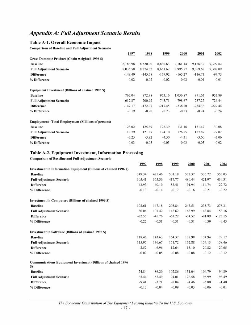
Full Adjustment Scenario The full adjustment scenario assumes that wages are reasonably flexible. When labor is released from industries suffering from the lower demand and output that is caused by the absence of the equipment leasing industry, wages fall sufficiently so that some of the initial employment reduction is restored and labor incomes consequently increase within the five-year study period. The induced impact on wages and incomes sets spending into motion so that some growth is also achieved over the study period. Consequently, the deleterious impact of removing equipment leasing from the economy is offset somewhat, and the economic impact that is measured represents a lower bound to the value of the industry. Overall Economic Contribution – Macroeconomic Indicators The results of this portion of the study indicate that real GDP would be permanently reduced by approximately $100 billion annually without the equipment leasing industry. The lost output is roughly 1% of 2002 real GDP and represents a lower bound estimate of the total value of the industry. (See Appendix A, Table A-1)

The strong link of the equipment leasing industry to capital spending on equipment is verified by the results of the Global Insight study. This portion of the study indicated that the absence of equipment leasing would result in a permanent reduction of $229 billion annually in equipment investment. (Appendix A, Table A-1.)

Without the availability of leasing, many firms throughout the economy would find it difficult or impossible to acquire capital equipment through purchase financing, and implicitly, business formation and growth would be curtailed. The extent of that curtailment is quantified through the number of jobs that would be lost in that kind of economy. In this portion of the study, we estimate that the number of jobs lost would be 3 million. (See Appendix A, Table A-1.) Composition of Equipment Investment The study looks deeper at equipment investment by quantifying the impact on component equipment investment categories, including total information processing, computer equipment, software, and telecommunications equipment. (See Appendix A, Table A-2.) We also looked at other key equipment components, including aircraft, transportation, industrial equipment, and other equipment investment. (See Appendix A, Table A-3.) The results are quite striking. Of the total $229-billion impact on equipment investment, over half ($122 billion) is concentrated in computer equipment. (See Appendix A, Table A-2) All industrial equipment categories—aircraft, especially transportation and industrial equipment—account for most of the balance of the effect. Employment Impacts – the Effect on Incomes and Employment By Industry

The estimated job impact in the full adjustment scenario was approximately 3 million jobs, as discussed above. In this scenario, a critical assumption has to do with how wages respond to surplus labor and how the economy responds in turn through job creation. In this case, with flexible wages, the initial reduction in employment induces wage cutting, which inevitably leads to greater hiring. However, real personal income and wages are left permanently lower by $338 billion (constant dollars) and $465 billion (current dollars), respectively. The baseline value of Personal Income per Worker is $61,550. However, in the Full Adjustment Scenario, with the substantial reduction in wages affecting personal income directly in addition to the 3 million job losses, the resulting value of Personal Income per worker falls to $60,260. We can see clearly that the impact of equipment leasing extends beyond providing for a greater number of jobs. The industry makes a direct contribution to labor and proprietor income.


Restricted Adjustment Scenario

In contrast to the full adjustment scenario, the restricted adjustment scenario makes the key assumption that wages are not flexible. It becomes more difficult for the economy to re-absorb labor excess labor created by the effects of removing the equipment leasing industry from the economy. Therefore, despite the relatively constant wage levels, job growth is diminished and follow-on income and spending growth are muted. The resulting economic value of the equipment leasing industry is at a maximum in this scenario.

Overall Economic Contribution – Macroeconomic Indicators

In this scenario, Global Insight evaluated the overall economic impact of the equipment leasing industry, as in the unrestricted adjustment case. In addition, it was also possible to decompose the impact to:

• The industry itself and all industries that are enveloped by leasing transactions, and • Spillover effects to the rest of the economy.

Our study indicates that absent the equipment leasing industry, the U.S. economy would suffer a permanent loss of $314 billion annually. (See Appendix B, Table B-1.) Most of this loss in output, on the order of $200 billion, would be borne directly by the industry and all related equipment supplier channels. (See Appendix C, Table C-1.) The balance would weave throughout the rest of the economy, which would suffer because of reductions in income and spending.

Composition of Equipment Investment

Over $225 billion in equipment investment would be lost annually in the absence of equipment leasing. (See Appendix B, Table B-1.) Most of this—$210 billion—would be concentrated in the industry and along the equipment supplier chain. (See Appendix B, Table B-2.)

Employment Impacts – the Effect on Incomes and Employment By Industry

The value of the equipment leasing industry is vividly shown in the results on employment and income. Over 5.0 million jobs—4.5 million in the industry and supplier industries—would be lost in the U.S. economy in the absence of the equipment leasing industry. (See Appendix B, Table B-1, and Appendix C, Table C-1.)

The income consequences to labor and proprietors in the United States would be huge, with real personal income lower by $375 billion annually. (See Appendix B, Table B-4.) Looking at the resulting value per worker, we can see that Personal Income per worker falls from the $61,550 value in the baseline to the lower $61,140 per worker. This is a somewhat higher figure than in the Full Adjustment Scenario because in this scenario, while the net loss of employment is larger, the reduction in wages is substantially smaller and therefore the impact on Personal Income is muted.

Participants in the industry and all related supplier industries would endure over $255 billion of this total. However, the spillover to the rest of the economy would still be on the order of $120 billion annually. (See Appendix C, Table C-4.)


Conclusions The Global Insight study was directed towards estimating the value and contribution of the equipment leasing industry to the U.S. economy through the application of an incremental analysis. Using our U.S. macro and industry models, we were able to create a five-year historical view of the U.S. economy without the equipment leasing industry. Our models enabled us to estimate the totality of the economic impact of the industry on all related industries in the equipment supply chain and on peripheral income and spending effects throughout the economy.

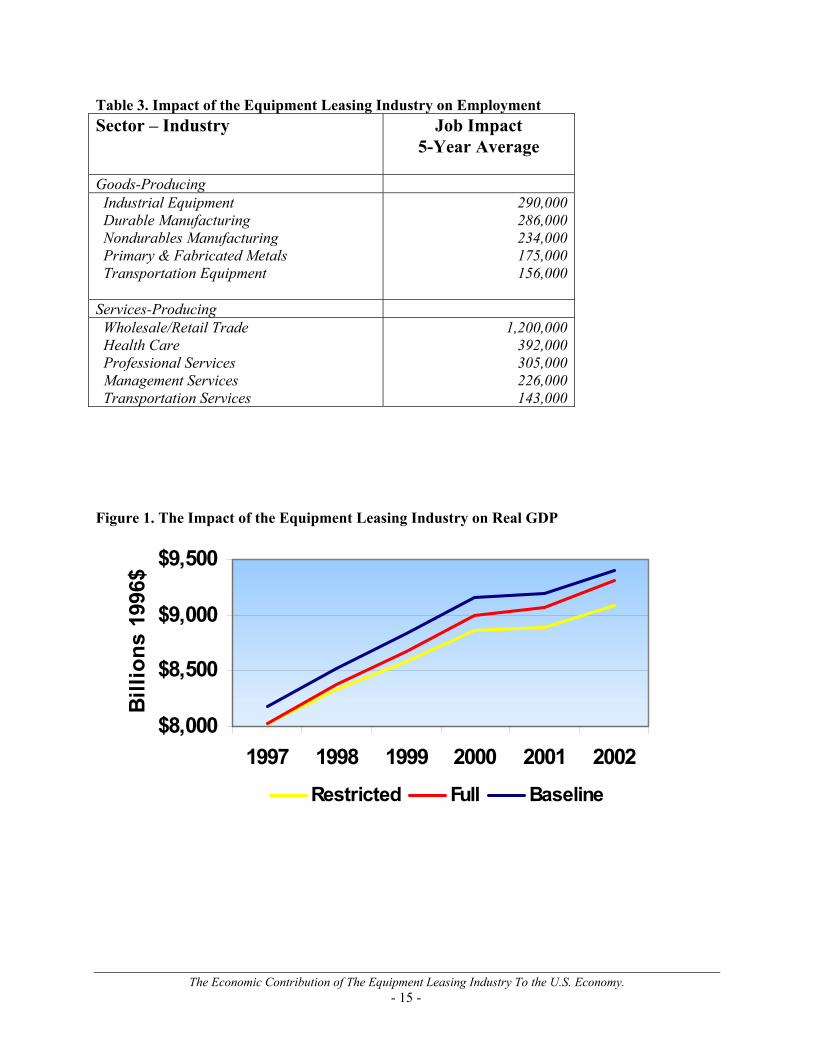
We measured the resulting impacts on three key aggregate indicators: real GDP, real equipment investment, and employment. (See Figures 1-3.) Based on alternative scenarios in our 1997-2002 study period, we quantitatively estimated that the equipment leasing industry:

• Contributed between $100 billion and $300 billion in real GDP annually. • Contributed between $227 billion and $229 billion in real equipment investment annually. • Contributed between 3 million and 5 million jobs.

The magnitudes are substantial. The impacts on real GDP range from 1-3% and are not trivial, particularly in light of the effect on real equipment investment. Equipment investment in the U.S. economy is on the order of $850 billion, roughly half of total investment. Our estimates suggest that over 25% of annual equipment investment is attributable to equipment leasing activity. What this additional contribution of capital investment drives is additional jobs. Our estimates imply that, on average, for just $60,000 of additional equipment investment generated through leasing, one job is created in the U.S. economy.

One of the more intriguing conclusions is given from looking at the impact on job creation across industries. Because of our ability to capture the inter-industry effects of equipment leasing, we were able to identify the impact on jobs across industries.5 We found that although the influence of leasing is spread across a number of industries, the effects are more concentrated in several key goods-producing and services-producing industries. Table 3 in the Tables and Graphs section exhibits the impact on jobs by industry based on the restricted scenario.6 What that table shows is that almost 70% of the jobs impact due to the equipment leasing industry is concentrated in ten industrial and services industries.

It can be inferred that these industries are the most sensitive to the availability of equipment leasing, and vice versa. That is, the impact of an expansion or contraction of equipment leasing would most likely be directed toward these industries. Similarly, any cyclical impact on these industries would directly influence the equipment leasing industry as well.

Measuring the value of the industry through key macroeconomic indicators gives a vivid and immediate picture of the importance of the industry in the U.S. economy. However, there are implications from the study that point to additional benefits that can also add to the economy. Central to these additional benefits is the conclusion that the principal value of the equipment leasing industry lies in its role of providing access to capital.

5 Because of the structure of the National Income and Product Accounts at the industry level, measuring output effects by industry is not possible. Therefore, we are only able to estimate the employment effects by industry. Because this is a quite reasonable metric, given the close correlation between output and employment across industries, acceptable inferences about growth and decline in industries can be made from looking at the employment data alone. 6 A full table of impacts across all industries can be obtained from the Equipment Leasing Association.


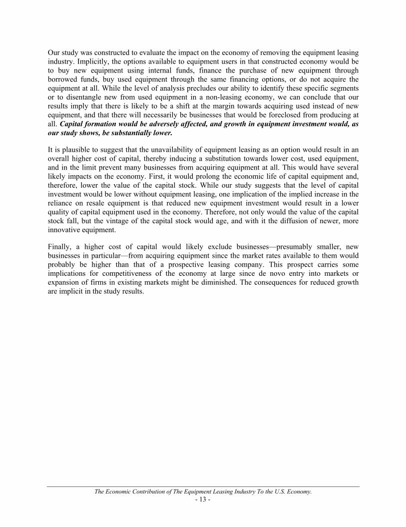
Our study was constructed to evaluate the impact on the economy of removing the equipment leasing industry. Implicitly, the options available to equipment users in that constructed economy would be to buy new equipment using internal funds, finance the purchase of new equipment through borrowed funds, buy used equipment through the same financing options, or do not acquire the equipment at all. While the level of analysis precludes our ability to identify these specific segments or to disentangle new from used equipment in a non-leasing economy, we can conclude that our results imply that there is likely to be a shift at the margin towards acquiring used instead of new equipment, and that there will necessarily be businesses that would be foreclosed from producing at all. Capital formation would be adversely affected, and growth in equipment investment would, as our study shows, be substantially lower.

It is plausible to suggest that the unavailability of equipment leasing as an option would result in an overall higher cost of capital, thereby inducing a substitution towards lower cost, used equipment, and in the limit prevent many businesses from acquiring equipment at all. This would have several likely impacts on the economy. First, it would prolong the economic life of capital equipment and, therefore, lower the value of the capital stock. While our study suggests that the level of capital investment would be lower without equipment leasing, one implication of the implied increase in the reliance on resale equipment is that reduced new equipment investment would result in a lower quality of capital equipment used in the economy. Therefore, not only would the value of the capital stock fall, but the vintage of the capital stock would age, and with it the diffusion of newer, more innovative equipment.

Finally, a higher cost of capital would likely exclude businesses—presumably smaller, new businesses in particular—from acquiring equipment since the market rates available to them would probably be higher than that of a prospective leasing company. This prospect carries some implications for competitiveness of the economy at large since de novo entry into markets or expansion of firms in existing markets might be diminished. The consequences for reduced growth are implicit in the study results.


Tables and Graphs Table 1. Equipment Investment, 5-Year Average Level, Top Ten Industries

Source: Bureau of Economic Analysis

Table 2. Equipment Leasing Volumes By Equipment Type

Source: Equipment Leasing Association

$ 75.068.361.051.946.740.631.124.724.223.3

WholesaleNon-bank FinancialTelecomBusiness ServicesReal EstateRetailAgriculturalCommercial BanksPower (Electric and Gas) ServicesAir Transportation

Equipment Investment5-Year Average

($Billions)Industry

$ 75.068.361.051.946.740.631.124.724.223.3

WholesaleNon-bank FinancialTelecomBusiness ServicesReal EstateRetailAgriculturalCommercial BanksPower (Electric and Gas) ServicesAir Transportation

Equipment Investment5-Year Average

($Billions)Industry

$205.6

$2.9$30.3$5.5

$14.3$59.4$21.2$3.3

$34.0$34.7

2002

2.8%

-20.8%11.7%19.0%

6.0%5.0%7.3%

----4.0%-0.7%

CAGR

$178.7Total Leasing Volumes

$9.3$17.4

$2.3$10.7$46.6$14.9

$0$41.6$35.9

CommunicationsComputerSoftwareOther Info ProcessingIndustrial EquipmentAircraftLight VehiclesOther TransportationOther Equipment

1997Equipment Type

$205.6

$2.9$30.3$5.5

$14.3$59.4$21.2$3.3

$34.0$34.7

2002

2.8%

-20.8%11.7%19.0%

6.0%5.0%7.3%

----4.0%-0.7%

CAGR

$178.7Total Leasing Volumes

$9.3$17.4

$2.3$10.7$46.6$14.9

$0$41.6$35.9

CommunicationsComputerSoftwareOther Info ProcessingIndustrial EquipmentAircraftLight VehiclesOther TransportationOther Equipment

1997Equipment Type


Table 3. Impact of the Equipment Leasing Industry on Employment Sector – Industry

Job Impact 5-Year Average

Goods-Producing Industrial Equipment Durable Manufacturing Nondurables Manufacturing Primary & Fabricated Metals Transportation Equipment

290,000286,000234,000175,000156,000

Services-Producing Wholesale/Retail Trade Health Care Professional Services Management Services Transportation Services

1,200,000392,000305,000226,000143,000

Figure 1. The Impact of the Equipment Leasing Industry on Real GDP

$8,000

$8,500

$9,000

$9,500

1997 1998 1999 2000 2001 2002

Bill

ions

199

6$

Restricted Full Baseline


Figure 2. The Impact of the Equipment Leasing Industry on Real Equipment Investment

Figure 3. The Impact of the Equipment Leasing Industry on Employment

$600$700$800$900

$1,000$1,100

1997 1998 1999 2000 2001 2002

Billi

ons

$199

6


115

120

125

130

135

1997 1998 1999 2000 2001 2002

Mill

ions



Appendix A: Full Adjustment Scenario Results

Table A-1. Overall Economic Impact Comparison of Baseline and Full Adjustment Scenario 1997 1998 1999 2000 2001 2002 Gross Domestic Product (Chain weighted 1996 $) Baseline 8,183.98 8,520.00 8,830.63 9,161.14 9,186.32 9,399.82 Full Adjustment Scenario 8,035.58 8,374.32 8,661.62 8,995.87 9,069.62 9,302.09 Difference -148.40 -145.68 -169.02 -165.27 -116.71 -97.73 % Difference -0.02 -0.02 -0.02 -0.02 -0.01 -0.01 Equipment Investment (Billions of chained 1996 $) Baseline 765.04 872.98 963.16 1,036.87 971.63 953.89 Full Adjustment Scenario 617.87 700.92 745.71 798.67 737.27 724.44 Difference -147.17 -172.07 -217.45 -238.20 -234.36 -229.44 % Difference -0.19 -0.20 -0.23 -0.23 -0.24 -0.24 Employment--Total Employment (Millions of persons) Baseline 123.02 125.69 128.39 131.16 131.47 130.08 Full Adjustment Scenario 119.79 121.87 124.10 126.85 127.87 127.02 Difference -3.23 -3.82 -4.30 -4.31 -3.60 -3.06 % Difference -0.03 -0.03 -0.03 -0.03 -0.03 -0.02

Table A-2. Equipment Investment, Information Processing Comparison of Baseline and Full Adjustment Scenario 1997 1998 1999 2000 2001 2002 Investment in Information Equipment (Billions of chained 1996 $) Baseline 349.34 425.46 501.18 572.37 536.72 553.03 Full Adjustment Scenario 305.41 365.36 417.77 480.44 421.97 430.31 Difference -43.93 -60.10 -83.41 -91.94 -114.74 -122.72 % Difference -0.13 -0.14 -0.17 -0.16 -0.21 -0.22 Investment in Computers (Billions of chained 1996 $) Baseline 102.61 147.18 205.84 243.51 235.73 278.31 Full Adjustment Scenario 80.06 101.42 142.62 168.99 143.84 153.16 Difference -22.55 -45.76 -63.22 -74.52 -91.89 -125.15 % Difference -0.22 -0.31 -0.31 -0.31 -0.39 -0.45 Investment in Software (Billions of chained 1996 $) Baseline 118.46 143.63 164.37 177.98 174.94 179.12 Full Adjustment Scenario 115.95 136.67 151.72 162.88 154.13 158.46 Difference -2.52 -6.96 -12.64 -15.10 -20.82 -20.65 % Difference -0.02 -0.05 -0.08 -0.08 -0.12 -0.12 Communications Equipment Investment (Billions of chained 1996 $) Baseline 74.84 86.20 102.86 131.04 104.79 94.89 Full Adjustment Scenario 65.44 82.49 94.01 126.58 98.99 93.49 Difference -9.41 -3.71 -8.84 -4.46 -5.80 -1.40 % Difference -0.13 -0.04 -0.09 -0.03 -0.06 -0.01


Table A-3. Equipment Investment, Capital Goods Comparison of Baseline and Full Adjustment Scenario 1997 1998 1999 2000 2001 2002 Investment in Aircraft (Billions of chained 1996 $) Baseline 14.74 19.74 28.15 29.07 29.48 18.97 Full Adjustment Scenario 9.35 9.07 13.56 16.96 13.66 10.30 Difference -5.38 -10.67 -14.59 -12.11 -15.82 -8.67 % Difference -0.37 -0.54 -0.52 -0.42 -0.54 -0.46 Investment in Transportation Equipment (Billions of chained 1996 $) Baseline 151.65 168.99 190.69 183.43 162.37 145.84 Full Adjustment Scenario 130.62 139.38 145.60 140.92 131.32 117.61 Difference -21.03 -29.61 -45.09 -42.51 -31.05 -28.23 % Difference -0.14 -0.18 -0.24 -0.23 -0.19 -0.19 Investment in Industrial Equipment (Billions of chained 1996 $) Baseline 139.78 146.25 147.09 159.52 153.18 145.07 Full Adjustment Scenario 93.93 95.17 92.87 88.39 97.54 90.24 Difference -45.85 -51.08 -54.22 -71.14 -55.64 -54.83 % Difference -0.33 -0.35 -0.37 -0.45 -0.36 -0.38 Other Equipment Investment (Billions of chained 1996 $) Baseline 125.38 136.83 135.81 141.71 138.00 135.98 Full Adjustment Scenario 89.78 105.09 99.41 106.63 97.44 100.96 Difference -35.61 -31.75 -36.41 -35.08 -40.56 -35.02 % Difference -0.28 -0.23 -0.27 -0.25 -0.29 -0.26 Table A-4. Personal Income and Wages Comparison of Baseline and Full Adjustment Scenario 1997 1998 1999 2000 2001 2002 Personal Income (Billions of chained 1996 $) Baseline 6828.84 7226.76 7420.28 7799.48 7905.84 8005.34 Full Adjustment Scenario 6659.34 6971.32 7082.49 7402.69 7533.64 7667.04 Difference -169.50 -255.44 -337.79 -396.79 -372.20 -338.30 % Difference -0.02 -0.04 -0.05 -0.05 -0.05 -0.04 Wages & Salaries (Billions of $) Baseline 3903.89 4191.34 4448.54 4807.90 4929.84 4974.26 Full Adjustment Scenario 3771.43 3993.13 4170.88 4450.06 4522.92 4509.19 Difference -132.46 -198.21 -277.66 -357.84 -406.92 -465.07 % Difference -0.03 -0.05 -0.06 -0.07 -0.08 -0.09


Appendix B: Restricted Adjustment Scenario Results, Total Impact

Table B-1. Overall Economic Impact Comparison of Baseline and Total Impact 1997 1998 1999 2000 2001 2002 Gross Domestic Product (Chain weighted 1996 $) Baseline 8183.98 8520.00 8830.63 9161.14 9186.32 9399.82 Total Impact 8028.17 8331.42 8578.88 8867.29 8893.99 9085.34 Difference -155.81 -188.58 -251.75 -293.85 -292.33 -314.48 % Difference -0.02 -0.02 -0.03 -0.03 -0.03 -0.03 Equipment Investment (Billions of chained 1996 $) Baseline 765.04 872.98 963.16 1036.87 971.63 953.89 Total Impact 617.36 697.05 740.10 793.55 734.10 726.94 Difference -147.68 -175.93 -223.06 -243.32 -237.53 -226.95 % Difference -0.19 -0.20 -0.23 -0.23 -0.24 -0.24 Employment--Total Employment (Millions of persons) Baseline 123.02 125.69 128.39 131.16 131.47 130.08 Total Impact 119.75 121.57 123.36 125.62 126.11 124.80 Difference -3.27 -4.12 -5.04 -5.54 -5.36 -5.28 % Difference -0.03 -0.03 -0.04 -0.04 -0.04 -0.04

Table B-2. Equipment Investment, Information Processing Comparison of Baseline and Total Impact 1997 1998 1999 2000 2001 2002 Investment in Information Equipment (Billions of chained 1996 $) Baseline 349.34 425.46 501.18 572.37 536.72 553.03 Total Impact 305.49 366.40 422.17 489.44 435.47 449.52 Difference -43.85 -59.06 -79.01 -82.93 -101.25 -103.52 % Difference -0.13 -0.14 -0.16 -0.14 -0.19 -0.19 Investment in Computers (Billions of chained 1996 $) Baseline 102.61 147.18 205.84 243.51 235.73 278.31 Total Impact 79.97 101.33 142.88 169.73 146.23 158.75 Difference -22.64 -45.85 -62.96 -73.78 -89.49 -119.56 % Difference -0.22 -0.31 -0.31 -0.30 -0.38 -0.43 Investment in Software (Billions of chained 1996 $) Baseline 118.46 143.63 164.37 177.98 174.94 179.12 Total Impact 116.12 137.58 154.26 167.70 161.22 169.09 Difference -2.34 -6.05 -10.11 -10.28 -13.73 -10.03 % Difference -0.02 -0.04 -0.06 -0.06 -0.08 -0.06 Communications Equipment Investment (Billions of chained 1996 $) Baseline 74.84 86.20 102.86 131.04 104.79 94.89 Total Impact 65.39 82.02 93.10 125.55 97.27 91.33 Difference -9.45 -4.18 -9.75 -5.49 -7.52 -3.56 % Difference -0.13 -0.05 -0.09 -0.04 -0.07 -0.04


Table B-3. Equipment Investment, Capital Goods Comparison of Baseline and Total Impact 1997 1998 1999 2000 2001 2002 Investment in Aircraft (Billions of chained 1996 $) Baseline 14.74 19.74 28.15 29.07 29.48 18.97 Total Impact 9.31 8.81 13.14 16.25 12.76 9.47 Difference -5.43 -10.93 -15.01 -12.82 -16.72 -9.50 % Difference -0.37 -0.55 -0.53 -0.44 -0.57 -0.50 Comparison of Baseline and Total Impact Investment in Transportation Equipment (Billions of chained 1996 $) Baseline 151.65 168.99 190.69 183.43 162.37 145.84 Total Impact 130.29 136.92 141.37 135.78 125.47 112.08 Difference -21.36 -32.07 -49.32 -47.65 -36.90 -33.76 % Difference -0.14 -0.19 -0.26 -0.26 -0.23 -0.23 Investment in Industrial Equipment (Billions of chained 1996 $) Baseline 139.78 146.25 147.09 159.52 153.18 145.07 Total Impact 93.89 94.30 90.38 84.23 92.57 85.14 Difference -45.89 -51.95 -56.71 -75.30 -60.61 -59.93 % Difference -0.33 -0.36 -0.39 -0.47 -0.40 -0.41 Other Equipment Investment (Billions of chained 1996 dollars) Baseline 125.38 136.83 135.81 141.71 138.00 135.98 Total Impact 89.60 103.90 97.30 104.00 94.67 98.73 Difference -35.78 -32.93 -38.51 -37.71 -43.33 -37.25 % Difference -0.29 -0.24 -0.28 -0.27 -0.31 -0.27 Table B-4. Personal Income and Wages Comparison of Baseline and Total Impact 1997 1998 1999 2000 2001 2002Personal Income (Billions of chained 1996 $) Baseline 6828.84 7226.76 7420.28 7799.48 7905.84 8005.34 Total Impact 6663.43 6971.79 7077.17 7392.06 7512.21 7630.39 Difference -165.41 -254.96 -343.11 -407.42 -393.63 -374.95% Difference -0.02 -0.04 -0.05 -0.05 -0.05 -0.05 Wages & Salaries (Billions of $) Baseline 3903.89 4191.34 4448.54 4807.90 4929.84 4974.26 Total Impact 3798.01 4064.30 4299.07 4652.78 4803.51 4859.49 Difference -105.88 -127.03 -149.47 -155.11 -126.33 -114.78% Difference -0.03 -0.03 -0.03 -0.03 -0.03 -0.02


Appendix C: Restricted Adjustment Scenario Results, Direct and Indirect Effects

Table C-1. Overall Economic Impact Comparison of Baseline and Direct & Indirect Impact 1997 1998 1999 2000 2001 2002 Gross Domestic Product (Chain weighted 1996 $) Baseline 8,183.98 8,520.00 8,830.63 9,161.14 9,186.32 9,399.82 Direct & Indirect Impact 8,040.46 8,350.19 8,621.24 8,942.67 8,974.80 9,199.46 Difference -143.52 -169.81 -209.39 -218.46 -211.52 -200.36 % Difference -0.02 -0.02 -0.02 -0.02 -0.02 -0.02 Equipment Investment (Billions of chained 1996 $) Baseline 765.04 872.98 963.16 1,036.87 971.63 953.89 Direct & Indirect Impact 618.13 697.47 742.93 805.93 749.62 746.79 Difference -146.91 -175.51 -220.23 -230.94 -222.01 -207.10 % Difference -0.19 -0.20 -0.23 -0.22 -0.23 -0.22 Employment--Total Employment (Millions of persons) Baseline 123.02 125.69 128.39 131.16 131.47 130.08 Direct & Indirect Impact 119.82 121.80 123.64 126.18 126.74 125.53 Difference -3.20 -3.90 -4.75 -4.98 -4.73 -4.55 % Difference -0.03 -0.03 -0.04 -0.04 -0.04 -0.03 Table C-2. Equipment Investment, Information Processing Comparison of Baseline and Direct & Indirect Impact 1997 1998 1999 2000 2001 2002 Investment in Information Equipment (Billions of chained 1996 $) Baseline 349.34 425.46 501.18 572.37 536.72 553.03 Direct & Indirect Impact 305.53 366.87 424.09 493.29 441.60 455.40 Difference -43.81 -58.59 -77.09 -79.09 -95.12 -97.63 % Difference -0.13 -0.14 -0.15 -0.14 -0.18 -0.18 Investment in Computers (Billions of chained 1996 $) Baseline 102.61 147.18 205.84 243.51 235.73 278.31 Direct & Indirect Impact 79.95 101.75 144.18 172.39 150.41 162.70 Difference -22.66 -45.43 -61.66 -71.13 -85.32 -115.61 % Difference -0.22 -0.31 -0.30 -0.29 -0.36 -0.42 Investment in Software (Billions of chained 1996 $) Baseline 118.46 143.63 164.37 177.98 174.94 179.12 Direct & Indirect Impact 116.11 137.54 155.09 170.48 165.76 173.53 Difference -2.35 -6.09 -9.27 -7.50 -9.18 -5.59 % Difference -0.02 -0.04 -0.06 -0.04 -0.05 -0.03 Communications Equipment Investment (Billions of chained 1996 $) Baseline 74.84 86.20 102.86 131.04 104.79 94.89 Direct & Indirect Impact 65.44 81.89 93.12 125.15 97.20 91.41 Difference -9.40 -4.32 -9.73 -5.89 -7.59 -3.48 % Difference -0.13 -0.05 -0.09 -0.04 -0.07 -0.04


Table C-3. Equipment Investment, Capital Goods Comparison of Baseline and Direct & Indirect Impact 1997 1998 1999 2000 2001 2002 Investment in Aircraft (Billions of chained 1996 $) Baseline 14.74 19.74 28.15 29.07 29.48 18.97 Direct & Indirect Impact 9.38 8.90 13.37 16.71 13.20 9.78 Difference -5.35 -10.83 -14.78 -12.36 -16.29 -9.19 % Difference -0.36 -0.55 -0.53 -0.43 -0.55 -0.48 Investment in Transportation Equipment (Billions of chained 1996 $) Baseline 151.65 168.99 190.69 183.43 162.37 145.84 Direct & Indirect Impact 131.12 138.29 143.80 140.69 130.07 117.53 Difference -20.53 -30.70 -46.89 -42.74 -32.31 -28.31 % Difference -0.14 -0.18 -0.25 -0.23 -0.20 -0.19 Investment in Industrial Equipment (Billions of chained 1996 $) Baseline 139.78 146.25 147.09 159.52 153.18 145.07 Direct & Indirect Impact 93.51 92.27 87.37 83.96 93.31 87.71 Difference -46.27 -53.98 -59.72 -75.57 -59.87 -57.36 % Difference -0.33 -0.37 -0.41 -0.47 -0.39 -0.40 Other Equipment Investment (Billions of chained 1996 $) Baseline 125.38 136.83 135.81 141.71 138.00 135.98 Direct & Indirect Impact 89.86 104.58 98.69 106.95 98.06 103.17 Difference -35.53 -32.25 -37.12 -34.76 -39.94 -32.80 % Difference -0.28 -0.24 -0.27 -0.25 -0.29 -0.24 Table C-4. Personal Income and Wages Comparison of Baseline and Direct & Indirect Impact 1997 1998 1999 2000 2001 2002 Personal Income (Billions of chained 1996 $) Baseline 6828.84 7226.76 7420.28 7799.48 7905.84 8005.34 Direct & Indirect Impact 6685.75 7017.96 7146.50 7490.12 7614.21 7750.20 Difference -143.09 -208.80 -273.77 -309.36 -291.63 -255.14 % Difference -0.02 -0.03 -0.04 -0.04 -0.04 -0.03 Wages & Salaries (Billions of $) Baseline 3903.89 4191.34 4448.54 4807.90 4929.84 4974.26 Direct & Indirect Impact 3819.66 4083.34 4311.47 4657.43 4782.30 4827.44 Difference -84.22 -108.00 -137.06 -150.46 -147.54 -146.82 % Difference -0.02 -0.03 -0.03 -0.03 -0.03 -0.03


Appendix D: Equipment Investment by Industry (Billions of 1996 $) 1997 1998 1999 2000 2001 2002 Wholesale trade 69466 70968 80888 87692 79207 77644Telephone and telegraph 51694 51825 61523 89344 67795 64436Nondepository institutions 59698 67265 80675 75250 67566 70091Business services 37667 48480 64534 68548 63134 56473Real estate 40339 48178 52954 52161 52879 49302Retail trade 34709 40251 40704 47927 44848 41688Electric services 19609 19628 23092 29457 33255 25008Agriculture, forestry, and fishing 31631 33570 28874 31144 32647 31573Transportation by air 18692 23214 25529 28308 30282 25205Commercial banks 22596 27279 28593 26447 24220 25827Auto repair, services, and parking 19131 20198 23915 25537 20499 21856Electronic and other electric equipment 18160 17459 16625 21408 20362 18803Insurance carriers 16155 19446 21780 22274 20003 19932Chemicals and allied products 20708 22277 20310 19374 18938 20321Construction 18324 21041 23725 21289 18631 20602Health services 12330 15027 15300 16068 17972 15339Other 12397 12763 17118 18151 17642 15614Mining 16563 16426 15705 15851 17423 16394Radio and television 13427 16736 19280 22190 16737 17674Industrial machinery and equipment 16188 17474 16770 17019 16260 16742Security and commodity brokers 8372 12237 14156 19054 15972 13958Food and kindred products 12566 13341 13999 13694 12966 13313Trucking and warehousing 20472 14006 12797 13637 10302 14243Motor vehicles and equipment 11960 13007 11020 9913 9300 11040Printing and publishing 8880 8543 9969 9698 9195 9257Paper and allied products 9954 10320 8017 9231 8914 9287Transportation services 5583 7906 8266 11383 8403 8308Rubber/miscellaneous plastics products 7819 8572 9084 8814 8098 8477Instruments and related products 6658 7786 7581 7837 7516 7476Fabricated metal products 7058 7792 7209 7454 6904 7283Holding and other investment offices 3180 5168 8817 7684 6570 6284Stone, clay, and glass products 5546 5926 6101 6695 6188 6091Sanitary services 4481 5330 6312 6174 6043 5668Primary metal industries 7142 7312 6341 6236 5828 6572Amusement and recreation services 2939 3514 4476 5710 5734 4475Gas services 6243 5545 6463 6739 5708 6140Hotels and other lodging places 4256 4052 5085 4360 4194 4389Petroleum and coal products 3816 3731 3215 3882 3861 3701Other transportation equipment 4449 5517 4920 3943 3802 4526Insurance agents, brokers, and service 2561 3786 3431 3610 3225 3323Legal services 2895 3265 3353 3452 3156 3224Lumber and wood products 2606 2822 2986 2920 2727 2812


(Billions of 1996 $) 1997 1998 1999 2000 2001 2002 Local and interurban passenger transit 1435 1893 2540 2567 2351 2157Motion pictures 5604 5448 3470 2623 2323 3894Railroad transportation 5056 5772 5653 3078 2293 4370Water transportation 2797 2567 2273 2232 2271 2428Textile mill products 3157 2990 2705 2312 2177 2668Miscellaneous repair services 2196 1353 1761 2334 2062 1941Personal services 2281 2273 2077 2120 1968 2144Furniture and fixtures 1208 1329 1410 1436 1342 1345Miscellaneous manufacturing industries 1127 1242 1246 1258 1171 1209Apparel and other textile products 972 1051 1109 1122 1064 1064Pipelines, except natural gas 1163 571 779 1150 1035 940Educational services 588 638 589 703 628 629Tobacco products 775 326 281 205 208 359Federal Reserve banks 153 160 245 223 201 196Leather and leather products 205 178 188 196 184 190


Appendix E: Overview of the Global Insight Macroeconomic Model GLOBAL INSIGHT Model of the U.S. Economy The Model’s Theoretical Position An Econometric Dynamic Equilibrium Growth Model: The Global Insight model strives to incorporate the best insights of many theoretical approaches to the business cycle: Keynesian, New Keynesian, Neoclassical, Monetarist, and Supply-side. In addition, the Global Insight model embodies the major properties of the Neoclassical growth models developed by Robert Solow. This structure guarantees that short-run cyclical developments will converge to robust long-run equilibrium. In growth models, the expansion rate of technical progress, the labor force, and the capital stock determine the productive potential of an economy. Both technical progress and the capital stock are governed by investment, which must be in balance with post-tax capital costs, available savings, and the capacity requirements of current spending. As a result, monetary and fiscal policies will influence both the short- and the long-term characteristics of such an economy through their impacts on national saving and investment. A modern model of output, prices, and financial conditions is melded with the growth model to present the detailed, short-run dynamics of the economy. In specific goods markets, the interactions of a set of supply and demand relations jointly determine spending, production, and price levels. Typically, the level of inflation-adjusted demand is driven by prices, income, wealth, expectations, and financial conditions. The capacity to supply goods and services is keyed to a production function combining the basic inputs of labor hours, energy usage, and the capital stocks of business equipment and structures, and government infrastructure. The “total factor productivity" of this composite of tangible inputs is driven by expenditures on research and development that produce technological progress. Prices adjust in response to gaps between current production and supply potential and to changes in the cost of inputs. Wages adjust to labor supply-demand gaps (indicated by a demographically adjusted unemployment rate), current and expected inflation (with a unit long-run elasticity), productivity, tax rates, and minimum wage legislation. The supply of labor positively responds to the perceived availability of jobs, to the after-tax wage level, and to the growth and age-sex mix of the population. Demand for labor is keyed to the level of output in the economy and the productivity of labor, capital, and energy. Because the capital stock is largely fixed in the short run, a higher level of output requires more employment and energy inputs. Such increases are not necessarily equal to the percentage increase in output because of the improved efficiencies typically achieved during an upturn. Tempering the whole process of wage and price determination is the exchange rate; a rise signals prospective losses of jobs and markets unless costs and prices are reduced. For financial markets, the model predicts exchange rates, interest rates, stock prices, loans, and investments interactively with the preceding GDP and inflation variables. The Federal Reserve sets the supply of reserves in the banking system and the fractional reserve requirements for deposits. Private sector demands to hold deposits are driven by national income, expected inflation, and the deposit interest yield relative to the yields offered on alternative investments. Banks and other thrift institutions, in turn, set deposit yields based on the market yields of their investment opportunities with comparable maturities and on the intensity of their need to expand reserves to meet legal


requirements. In other words, the contrast between the supply and demand for reserves sets the critical short-term interest rate for interbank transactions, the federal funds rate. Other interest rates are keyed to this rate, plus expected inflation, Treasury borrowing requirements, and sectoral credit demand intensities. The old tradition in macroeconomic model simulations of exogenous fiscal or environmental policy changes was to hold the Federal Reserve’s supply of reserves constant at baseline levels. While this approach makes static analysis easier in the classroom, it sometimes creates unrealistic policy analyses when a dynamic model is appropriate. In the Global Insight model, “monetary policy” is defined by a set of targets, instruments, and regular behavioral linkages between targets and instruments. The model user can choose to define unchanged monetary policy as unchanged reserves, or as an unchanged reaction function in which interest rates or reserves are changed in response to changes in such policy concerns as the price level and the unemployment rate. Monetarist Aspects: The model pays due attention to valid lessons of monetarism by carefully representing the diverse portfolio aspects of money demand and by capturing the central bank's role in long-term inflation phenomena. The private sector may demand money balances as one portfolio choice among transactions media (currency, checkable deposits), investment media (bonds, stocks, short-term securities), and durable assets (homes, cars, equipment, structures). Given this range of choice, each medium's implicit and explicit yield must match expected inflation, offset perceived risk, and respond to the scarcity of real savings. Money balances provide benefits by facilitating spending transactions and can be expected to rise nearly proportionately with transactions requirements unless the yield of an alternative asset changes. Now that even demand deposit yields can float to a limited extent in response to changes in Treasury bill rates, money demand no longer shifts quite as sharply when market rates change. Nevertheless, the velocity of circulation (the ratio of nominal spending to money demand) is still far from stable during a cycle of monetary expansion or contraction. The simple monetarist link from money growth to price inflation or nominal spending is, therefore, considered invalid as a rigid short-run proposition. Equally important, as long-run growth models demonstrate, induced changes in capital formation can also invalidate a naive long-run identity between monetary growth and price increases. Greater demand for physical capital investment can enhance the economy's supply potential in the event of more rapid money creation or new fiscal policies. If simultaneous, countervailing influences deny an expansion of the economy's real potential, the model will translate all money growth into a proportionate increase in prices, rather than in physical output. “Supply-Side" Economics: Since 1980, “supply-side" political economists have pointed out that the economy's growth potential is sensitive to the policy environment. They focused on potential labor supply, capital spending, and savings impacts of tax rate changes. The Global Insight model embodies supply-side hypotheses to the extent supportable by available data, and this is considerable in the many areas that supply-side hypotheses share with long-run growth models. These features, however, have been fundamental ingredients of our model since 1976.


Rational Expectations: As the rational expectations school has pointed out, much of economic decision-making is forward looking. For example, the decision to buy a car or a home is not only a question of current affordability, but also one of timing. The delay of a purchase until interest rates or prices decline has become particularly common since the mid-1970s, when both inflation and interest rates were very high and volatile. Consumer sentiment surveys, such as those conducted by the University of Michigan Survey Research Center, clearly confirm this speculative element in spending behavior. However, households can be shown to base their expectations, to a large extent, on their past experiences: they believe the best guide to the future is an extrapolation of recent economic conditions and the changes in those conditions. Consumer sentiment about whether this is a “good time to buy" can, therefore, be successfully modeled as a function of recent levels and changes in employment, interest rates, inflation, and inflation expectations. Similarly, inflation expectations (influencing financial conditions) and market strength expectations (influencing inventory and capital spending decisions) can be modeled as functions of recent rates of increase in prices and spending. This largely retrospective approach is not, of course, wholly satisfactory to pure adherents to the rational expectations doctrine. In particular, this group argues that the announcement of macroeconomic policy changes would significantly influence expectations of inflation or growth prior to any realized change in prices or spending. If an increase in government expenditures is announced, the argument goes, expectations of higher taxes to finance the spending might lead to lower consumer or business spending in spite of temporarily higher incomes from the initial government spending stimulus. A rational expectations theorist would, thus, argue that multiplier effects will tend to be smaller and more short-lived than a mainstream economist would expect. These propositions are subject to empirical evaluation. Our conclusions are that expectations do play a significant role in private sector spending and investment decisions; but, until change has occurred in the economy, there is very little room for significant changes in expectations in advance of an actual change in the variable about which the expectation is formed. The rational expectations school thus correctly emphasizes a previously understated element of decision-making, but exaggerates its significance for economic policy-making and model building. The Global Insight Model allows a choice in this matter. On the one hand, the user can simply accept Global Insight's judgments and let the model translate policy initiatives into initial changes in the economy, simultaneous or delayed changes in expectations, and subsequent changes in the economy. On the other hand, the user can manipulate the clearly identified expectations variables in the model, i.e., consumer sentiment and inflation expectations. For example, if the user believes that fear of higher taxes would subdue spending, he/he could reduce the consumer sentiment index. Such experiments can be made “rational" through model iterations that bring the current change in expectations in line with future endogenous changes in employment, prices, or financial conditions. Theory as a Constraint: The conceptual basis of each equation in the Global Insight model was thoroughly worked out before the regression analysis was initiated. The list of explanatory variables includes a carefully selected set of demographic and financial inputs. Each estimated coefficient was then thoroughly tested to be certain that it meets the tests of modern theory and business practice. This attention to equation specification and coefficient results has eliminated the “short circuits" that can occur in evaluating a derivative risk or an alternative policy scenario. Because each equation will stand up to a thorough inspection, the Global Insight Model is a reliable analytical tool and can be


used without excessive iterations. The model is not a black box: it functions like a personal computer spreadsheet in which each interactive cell has a carefully computed, theoretically consistent entry and, thus, performs logical computations simultaneously. Major Sectors The Global Insight model captures the full simultaneity of the U.S. economy, forecasting over 1,200 concepts spanning final demands, aggregate supply, prices, incomes, international trade, industrial detail, interest rates, and financial flows. Chart 1 summarizes the structure of the eight interactive sectors (noted in Roman numerals). The following discussion presents the logic of each sector and the significant interactions with other sectors. Spending—Consumer: The domestic spending (I), income (II), and tax policy (III) sectors model the central circular flow of behavior as measured by the national income and product accounts. If the rest of the model were “frozen," these blocks would produce a Keynesian system similar to the models pioneered by Tinbergen and Klein, except that neoclassical price factors have been imbedded in the investment and other primary demand equations. Consumer spending on durable goods is divided into 11 categories: 2 light vehicles categories; net purchases of used carsl; motor-vehicle parts; recreational vehicles; computers; software; other household equipment and furnishings; opthalmic and orthopedic products, and “other." Spending on nondurable goods is divided into 9 categories: 3 food categories; clothing and shoes; gasoline and oil; fuel oil and coal; tobacco; drugs; and “other." Spending on services is divided into 17 categories: housing; transportation; 6 household operation subcategories; 5 transportation categories; medical; recreation; 2 personal business service categories; and “other." In nearly all cases, real consumption expenditures are motivated by real income and the user price of a particular category relative to the prices of other consumer goods. Durable and semidurable goods are also especially sensitive to current financing costs and consumer speculation on whether it is a “good time to buy." The University of Michigan Survey of Consumer Sentiment monitors this last influence, with the index itself modeled as a function of current and lagged values of inflation, unemployment, and the prime rate. Spending—Business Investment: Business spending includes six fixed investment categories: four information processing equipment categories; industrial equipment; two transportation equipment categories; other producers’ durable equipment; four building categories; mining and petroleum structures; public utility structures; and miscellaneous. Equipment and (non-utility and non-mining) structures spending components are determined by their specific effective post-tax capital costs, capacity utilization, and replacement needs. The cost terms are sophisticated blends of post-tax debt and equity financing costs (offset by expected capital gains) and the purchase price of the investment good (offset by possible tax credits and depreciation-related tax benefits). This updates the well-known work of Dale Jorgenson, Robert Hall, and Charles Bischoff. Given any cost/financing environment, the need to expand capacity is monitored by recent growth in national goods output weighted by the capital intensity of such production. Public utility structure expenditures are motivated by similar concepts, except that the output terms are restricted to utility output, rather than total national goods output. Net investment in mining and petroleum structures responds to movements in real domestic oil prices and to oil and natural gas production.


I.DOMESTICSPENDINGHouseholdBusiness

Government

VII.SIMULATED SUPPLY

POTENTIALR&D

Labor ForceCapital Stock

Foreign Sources

VI.INFLATION

WagesCapitalEnergy

ConsumerWholesale

Foreign

II.DOMESTIC INCOME

WagesProfitsInterest

Rent

VIII. EXPECTATIONS

Consumer Confidence

Future Inflation Future Output

IV. INTERNATIONAL

EXCHANGE RATE

EXPORTS IMPORTS

INTERESTRATES

DEMANDFOR

MONEY ANDCREDIT

SUPPLY OF

CREDIT Federal Reserve

V. FINANCIAL

III.TAX

POLICY

Trade Deficits Inflation Interest Rates

Investment, Real Wages, Energy Use

The Global Insight Model of the U.S. Economy Overview

Chart 1. Overview of the Global Insight Model of the U.S. Economy


Inventory demand is the most erratic component of GDP, reflecting the pro-cyclical, speculative nature of private sector accumulation during booms and decumulation during downturns. The forces that drive the five nonfarm inventory categories are changes in spending, short-term interest rates and expected inflation, surges in imports, and changes in capacity utilization or the speed of vendor deliveries. Surprise increases in demand lead to an immediate drawdown of stocks and then a rebuilding process over the next year; the reverse naturally holds for sudden reductions in final demand. Inventory demands are sensitive to the cost of holding the stock, measured by such terms as interest costs adjusted for expected price increases and by variables monitoring the presence of bottlenecks. The cost of a bottleneck that slows delivery times is lost sales. An inventory spiral can, therefore, be set in motion when all firms accelerate their accumulation during a period of strong growth but then try to deplete excessive inventories when the peak is past. Spending—Residential Investment: The residential investment sector of the model includes two housing starts (single- and multi-family starts) and three housing sales categories (new and existing single-family sales and new single-family units for sale). Housing starts and sales, in turn, drive investment demand in five GDP account categories: single-family housing; multi-family housing; improvements; miscellaneous; and residential equipment. Residential construction is typically the first sector to turn down in a recession and the first to rebound in a recovery. Moreover, the magnitude of the building cycle is often the key to that of the subsequent macroeconomic cycle. The housing sector of the Global Insight Model explains new construction as a decision primarily based on the after-tax cost of home ownership relative to disposable income. This cost is estimated as the product of the average new home price adjusted for changes in quality, and the mortgage rate, plus operating costs, property taxes, and an amortized down payment. “Lever variables" allow the model user to specify the extent to which mortgage interest payments, property taxes, and depreciation allowances (for rental properties) produce tax deductions that reduce the effective cost. The equations also include a careful specification of demographic forces. After estimating the changes in the propensity for specific age-sex groups to form independent households, the resulting “headship rates" were multiplied by corresponding population statistics to estimate the trend expansion of single- and multi-family households. The housing equations were then specified to explain current starts relative to the increase in trend households over the past year, plus pent-up demand and replacement needs. The basic phenomenon being scrutinized is, therefore, the proportion of the trend expansion in households whose housing needs are met by current construction. The primary determinants of this proportion are housing affordability, consumer confidence, and the weather. Actual construction spending in the GDP accounts is the value of construction “put in place" in each period after the start of construction (with a lag of up to six quarters in the case of multi-family units), plus residential improvements and brokerage fees. Spending—Government: The last sector of domestic demand for goods and services, that of the government, is largely exogenous (user determined) at the federal level and endogenous (equation determined) at the state and local level. The user sets the real level of federal nondefense and defense purchases (for compensation, consumption of fixed capital, CCC inventory change, other consumption, and gross investment), medical and non-medical transfer payments, and medical and non-medical grants to state and local governments. The model calculates the nominal values through multiplication by the relevant estimated prices. Transfers to foreigners, wage accruals, and subsidies (agricultural, housing, and other) are also specified by the user, but in nominal dollars. One category


of federal government spending—net interest payments—is determined within the model because of its dependence on the model’s financial and tax sectors. Net federal interest payments are determined by the level of privately-held federal debt, short- and long-term interest rates, and the debt's maturity. The presence of a large and growing deficit imposes no constraint on federal spending. This contrasts sharply with the state and local sector, where legal requirements for balanced budgets mean that declining surpluses or emerging deficits produce both tax increases and reductions in spending growth. State and local purchases (for compensation, consumption of fixed capital, other consumption, and construction) are also driven by the level of federal grants (due to the matching requirements of many programs), population growth, and trend increases in personal income. Income: Domestic spending, adjusted for trade flows, defines the economy's value added or gross national product (GNP) and gross domestic product (GDP). Because all value added must accrue to some sector of the economy, the expenditure measure of GNP also determines the nation's gross income. The distribution of income among households, business, and government is determined in sectors II and III of the model. Pre-tax income categories include private and government wages, corporate profits, interest, rent, and entrepreneurial returns. Each pre-tax income category except corporate profits is determined by some combination of wages, prices, interest rates, debt levels, and capacity utilization or unemployment rates. In some cases such as wage income, these are identities based on previously calculated wage rates, employment, and hours per week. Profits are logically the most volatile component of GNP on the income side. When national spending changes rapidly, the contractual arrangements for labor, borrowed funds, and energy imply that the return to equity holders is a residual that will soar in a boom and collapse in a recession. The model reflects this by calculating wage, interest, and rental income as thoroughly reliable near-identities (e.g., wages equal average earnings multiplied by hours worked) and then subtracting each non-profit item from national income to solve for profits. Taxes: Since post-tax, rather than pre-tax, incomes drive expenditures, each income category must be taxed at an appropriate rate; therefore, the model tracks personal, corporate, payroll, and excise taxes separately. Users may set federal tax rates; tax revenues are then simultaneously forecast as the product of the rate and the associated pre-tax income components. However, the model automatically adjusts the effective average personal tax rate for variations in inflation and income per household, and the effective average corporate rate for credits earned on equipment, utility structures, and research and development. Substitutions or additions of “flat” taxes and value-added taxes for existing taxes are accomplished with specific tax rates and new definitions of tax bases. As appropriate, these are aggregated into personal, corporate, or excise tax totals. State and local corporate profits and social insurance (payroll) tax rates are exogenous in the model, while personal income and excise taxes are fully endogenous: the model makes reasonable adjustments automatically to press the sector toward the legally required approximate budget balance. The average personal tax rate rises with income and falls with the government operating surplus. Property and sales taxes provide the bulk of state excise revenue and reflect changes in oil and natural gas production, gasoline purchases, and retail sales, as well as revenue requirements. The feedback from expenditures to taxes and taxes to expenditures works quite well in reproducing both the secular growth of the state and local sector and its cyclical volatility.


International: The international sector (IV) is a critical, fully simultaneous block that can either add or divert strength from the central circular flow of domestic income and spending. Depending on the prices of foreign output, the U.S. exchange rate, and competing domestic prices, imports capture varying shares of domestic demand. Depending on similar variables and the level of world gross domestic product, exports can add to domestic spending on U.S. production. The exchange rate itself responds to international differences in inflation, interest rates, trade deficits, and capital flows between the United States and its competitors. In preparing forecasts, Global Insight's U.S. Economic Service and the World Service collaborate in determining internally consistent trade prices and volumes, interest rates, and financial flows. Eight categories of goods and one services category are separately modeled for both imports and exports, with one additional goods category for oil imports. For example, export and import detail for business machines is included as a natural counterpart to the inclusion of the office equipment component of producers' durable equipment spending. The business machines detail allows more accurate analysis because computers are rapidly declining in effective quality-adjusted prices relative to all other goods, and because such equipment is rising so rapidly in prominence as businesses push ahead with new production and information processing technologies. Investment income flows are also explicitly modeled. The stream of huge current account deficits incurred by the United States has important implications for the U.S. investment income balance. As current account deficits accumulate, the U.S. net international investment position and the U.S. investment income balance deteriorate. U.S. foreign assets and liabilities are, therefore, included in the model, with the current account deficit determining the path of the net investment position. The reactions of overseas prices, interest rates, and GDP to U.S. development are robust and automatic. In the case of dollar depreciation, for example, U.S. activity may expand at the expense of foreign activity and U.S. inflation may rise while the rate in other countries slows. Financial: The use of a detailed financial sector (V) and of interest rate and wealth effects in the spending equations recognizes the importance of credit conditions on the business cycle and on the long-run growth prospects for the economy. Interest rates, the key output of this sector, are modeled as a term structure, pivoting off the federal funds rate. As noted earlier, the model gives the user the flexibility of using the supply of reserves as the key monetary policy instrument, reflecting the Federal Reserve's open market purchases or sales of Treasury securities, or using a reaction function as the policy instruction. If the supply of reserves is chosen as the policy instrument, the federal funds rate depends on the balance between the demand and supply of reserves to the banking system. Banks and other thrift institutions demand reserves to meet the reserve requirements on their deposits and the associated (exogenous) fractional reserve requirements. The private sector, in turn, demands deposits of various types, depending on current yields, income, and expected inflation. If the reaction function is chosen as the monetary policy instrument, the federal funds rate is determined in response to changes in such policy concerns as inflation and unemployment. The reaction function recognizes that monetary policy seeks to stabilize prices (or to sustain a low


inflation rate) and to keep the unemployment rate as close to the natural rate as is consistent with the price objective. A scenario designed to display the impact of a fiscal or environmental policy change in the context of “unchanged” monetary policy is arguably more realistic when “unchanged” or traditional reactions to economic cycles are recognized, than when the supply of reserves is left unchanged. Longer-term interest rates are driven by shorter-term rates as well as factors affecting the slope of the yield curve. In the Global Insight model, such factors include inflation expectations, government borrowing requirements, and corporate financing needs. The expected real rate of return varies over time and across the spectrum of maturities. An important goal of the financial sector is to capture both the persistent elements of the term structure and to interpret changes in this structure. Twenty-eight interest rates are covered in order to meet client needs regarding investment and financial allocation strategies. Inflation: Inflation (VI) is modeled as a carefully controlled, interactive process involving wages, prices, and market conditions. Equations embodying a near accelerationist point of view produce substantial secondary inflation effects from any initial impetus such as a change in wage demands or a rise in foreign oil prices. Unless the Federal Reserve expands the supply of credit, real liquidity is reduced by any such shock; given the real financial interactions described earlier, this can significantly reduce growth. The process also works in reverse: a spending shock can significantly change wage-price prospects and then have important secondary impacts on financial conditions. Inspection of the simulation properties of the Global Insight model, including full interaction among real demands, inflation and financial conditions, confirms that the model has moved toward central positions in the controversy between fiscalists and monetarists, and in the debates among neoclassicists, institutionalists, and “rational expectationists." The principal domestic cost influences are labor compensation, nonfarm productivity (output per hour), and foreign input costs. The latter are driven by the exchange rate, the price of oil, and foreign wholesale price inflation. Excise taxes paid by the producer are an additional cost fully fed into the pricing decision. This set of cost influences drives each of the 19 industry-specific producer price indexes, in combination with a demand pressure indicator and appropriately weighted composites of the other 18 producer price indexes. In other words, the inflation rate of each industry price index is the reliably weighted sum of the inflation rates of labor, energy, imported goods, and domestic intermediate goods, plus a variable markup reflecting the intensity of capacity utilization or the presence of bottlenecks. If the economy is in balance—with an unemployment rate near 5%, manufacturing capacity utilization steady near 80-85%, and foreign influences neutral—then prices will rise in line with costs and neither will show signs of acceleration or deceleration. Supply: The first principle of the market economy is that prices and output are determined simultaneously by the factors underlying both demand and supply. As noted previously, the “supply-siders" have not been neglected in the Global Insight model; indeed, substantial emphasis on this side of the economy (VII) was incorporated as early as 1976. In the Global Insight model, aggregate supply (or potential GDP excluding the energy sector) is estimated by a Cobb-Douglas production function, which combines factor input growth and improvements in total factor productivity. Factor input equals a weighted average of labor, business fixed capital, public infrastructure, and energy provided by the energy sector. Based on each factor's historical share of total input costs, the elasticity of potential output with respect to labor is 0.64 (i.e., a 1.00% increase in the labor supply increases potential GDP 0.64%); the business capital elasticity is 0.26, the infrastructure elasticity is


0.02, and the energy elasticity is 0.07. Factor supplies are defined by estimates of the full employment labor force, the full employment capital stock, end-use energy demand, and the stock of infrastructure. Total factor productivity depends on the stock of research and development capital and trend technological change. The energy sector employs its own capital and labor. Potential GDP is the sum of the energy and non-energy sector outputs, less energy imports. Taxation and other government policies influence labor supply and all investment decisions, thereby linking tax changes to changes in potential GDP. An expansion of potential first reduces prices and then credit costs, and thus spurs demand. Demand rises until it equilibrates with the potential output. Thus, the growth of aggregate supply is the fundamental constraint on the long-term growth of demand. Inflation, created by demand that exceeds potential GDP or by a supply-side shock or excise tax increase, raises credit costs and weakens consumer sentiment, thus putting the brakes on aggregate demand. Expectations: The contributions to the model and its simulation properties of the rational expectations school are as rich as the data will support. Expectations (Sector VIII) impact several expenditure categories in the Global Insight model, but the principal nuance relates to the entire spectrum of interest rates. Shifts in price expectations or the expected capital needs of the government are captured through price expectations and budget deficit terms, with the former impacting the level of rates throughout the maturity spectrum, and the latter impacting intermediate and long-term rates, hence affecting the shape of the yield curve. On the expenditure side, inflationary expectations impact consumption via consumer sentiment, while growth expectations affect business investment.


Appendix F: Overview of the Global Insight Industry Model INDUSTRIAL ANALYSIS SERVICE MODEL OVERVIEW

Overview The Industrial Analysis Service model is a combination input-output/stochastic model of activity in 128 U.S. industries.

The model forecasts demand, industrial production indexes, shipments, value of production, inventories, prices, employment, productivity, average hourly earnings, material cost, and operating margin for each manufacturing industry.

Value of production, prices, employment, productivity, average hourly earnings, material cost, and operating margin are also forecast for nonmanufacturing sectors.

The industry aggregation follows the 73 manufacturing industries reported by the Department of Commerce in its monthly shipments, orders, and inventories release—basically a three–digit SIC aggregation and a largely two-digit scheme for 55 nonmanufacturing industries. The input–output block in the model translates macroeconomic forecasts from Global Insight’s short- and long-term macroeconomic model into demand by industry. These I-O tables are used for the calculation of input cost by industry, used in forecasting prices, and in the calculation of material costs. All other model concepts are forecasted by statistical equations and identities. The model forecasts quarterly frequency industry indicators, and forecasts are updated each month. Historical data for the most part are monthly series released by various government agencies, which are typically up to date within two months of forecast time. All data, unless otherwise specified, are seasonally adjusted annual rates.

The Input/Output Block Standard input–output analysis is carried out in two steps. First, the vector of economic expenditures from the macroeconomic model (the components of GDP) is converted into a vector of industrial deliveries to final demand. This conversion is represented for any time period as: F = H * G where: F = vector of industrial deliveries to final demand H = benchmark bridge matrix recording the industrial composition of each expenditure category G = vector of real final expenditure components of GNP A fixed bridge matrix, constructed from the 1992 input-output tables and workfiles (the most recent complete information released by the Bureau of Economic Analysis) is used in this conversion. Once the final demand vector, F, has been calculated, standard input-output techniques are used to derive estimates of the industrial output required to produce this bill of goods for final use. According to the basic input-output model, intermediate inputs, industrial deliveries to final demand, and gross output are related as follows: A * X + F = X


where: A = matrix of direct input coefficients describing the amount of each input industry’s product

required per unit of industry output X = vector of gross output by industry This equation can be considered an equilibrium condition that total demand equals total supply. The product A * X is equal to intermediate demand, and F is equal to final demand. The sum of the two is total demand, which, in equilibrium, is equal to total supply, or production. Following standard input-output conventions, it is assumed that the technology of production as reflected by the matrix of direct input coefficients, A, remains relatively stable over time. In addition, production processes are assumed to be linear and exhibit constant returns to scale with no possibility for substitution among inputs. However, these restrictions apply for the calculation of demand by industry only—equations for actual shipments and production include factors that offset these restrictive assumptions statistically. The basic input-output equation is then solved for output: Inverse(I – A) * F = X This equation describes the relationship between final demand and industrial output levels that would be required to deliver this bill of goods under the restrictive assumptions detailed above. The vector X should equal total demand and supply for each industry, in equilibrium.

Industrial Production The industrial production indexes in the model, about 150 two- and three-digit industry groupings, are quarterly averages of the Federal Reserve Board’s indexes over history. A number of unpublished series, not printed in the Fed’s monthly release, are forecast in order to provide complete coverage of the disaggregate sectors required to weight up to aggregates. Disaggregate industrial production indexes are estimated as a function of total demand for the input-output analysis, cyclical variables, and a time trend. The functional form used imposes a unitary elasticity on the demand term, which embodies most of the explanatory power in the equations. The additional, nondemand terms are included in the equation to explain the patterns not well accounted for by the input-output model and its demand indicators—cyclicality and technological change.

Macroeconomic variables feed down into the industry output equations through demand, but these weighted demand terms are in most cases smoother and less cyclical than industrial production indexes. Therefore, cyclical variables, such as capacity utilization, housing starts, or interest rates, are included in most equations. Cyclical variables were chosen with care to reflect the appropriate business cycle for each industry.

The use of constant 1992 input-output tables in the construction of total demand becomes less accurate the farther from the base year the estimates go. This is because shifts in relative prices for inputs, as well as other factors, can change the technological processes used to manufacture goods in the long run. To account for this slowly changing divergence between input-output coefficients and actual production processes, a simple time trend is used in many model equations that use input-output concepts.


The standard equation specification for industrial production indexes is: LOG(JIPind/GOODind_96) = F (LOG(Cyclical variable), trend) where: JIPind = industrial production index, industry ind GOODind_96 = total input-output demand, industry ind trend = time trend dummy variable Aggregate industrial production indexes are chain-weighted averages of the disaggregates, using Federal Reserve Board weight. These equations are coded in the model with add-factors sometimes required to eliminate a jump-off problem in the first forecast period due to an inexact fit in the last quarterly—frequency, seasonally—adjusted historical period.

Shipments Industry shipments are measured in billions of current and constant dollars and are available for each of the 73 manufacturing industries in the Industrial Analysis Service model. The current dollar historical series are quarterly averages of the Department of Commerce’s value of shipments data from its monthly shipments, orders, and inventories release, which are then converted to annual rates by multiplying by 12. Constant dollar historical values are the current dollar series deflated using each industry’s industry price index. Constant-dollar shipments are forecast with equations that have exactly parallel specifications to those for industrial production indexes. LOG(GOOind_96/GOODind_96) = F (LOG(Cyclical variable), trend) where: GOOind_96 = constant-dollar value of shipments, industry ind GOODind_96 = total input-output demand, industry ind trend = time trend dummy variable Current–dollar forecasts are the constant dollar series inflated using industry price indexes. GOOind = GOOind_96 * PGOOind /100 where: GOOind = current–dollar value of shipments, industry ind PGOOind = industry price index, industry ind

Value of Production for Nonmanufacturing Value of industry production for the manufacturing industries is constructed over history on a quarterly basis as value of shipments plus the change in the value of finished goods inventories at an annual rate. This identity holds for both current and constant dollar statistics and is also the method used for forecasting. For nonmanufacturing industries, value of production is the main activity indicator available, and historical data are derived from a number of different sources. The common criterion for the data, however, is that conceptually it be as close as possible to the measure of value of production for the manufacturing industries—it always measures total gross output, rather than value added—and the


current-dollar measure is roughly equivalent to revenue. The standard identity between current dollar and constant dollar output and the industry price index always holds. Forecasts of nonmanufacturing value of production are calculated from equations of the same form as the manufacturing industrial production and shipments equations: LOG(GOOind_96/GOODind_96) = F (LOG(Cyclical variable), trend) where: GOOind_96 = value of production, nonmanufacturing industry ind GOODind_96 = total input-output demand, industry ind trend = time trend dummy variable

Employment Employment is measured in millions and is reported at annual rates. Historical data are constructed from the Bureau of Labor Statistics’ monthly employment and earnings release. They are forecast for all 73 manufacturing industries and as many of the 53 nonmanufacturing industries for which we could find data. Equations for employment are estimated as inverted production function, with employment as the dependent variables. Independent variables are basically industry real wages rate and constant dollar activity variables. LOG(EMEind) = F(LOG(MovAvg(4, GOOind_96)), Trend, Aggregate Productivity) where: EMEind = employment, industry ind GOOind_96 = value of production, industry ind WRHPind = average hourly earnings, industry ind PGOOind = industry price index, industry ind Productivity is an identity in both the historical and forecast periods, calculated as value of production divided by employment. RAOHRind = (GOOind / EMEind) where: RAOHRMind = labor productivity, industry ind

Average Hourly Earnings Average hourly earnings are current dollar hourly wages averaged into quarterly data from the Bureau of Labor Statistics’ monthly employment and earnings release. All two-digit manufacturing industries are forecast, as well as many three-digit, and major industries in the nonmanufacturing area are also covered. Forecasts of average hourly earnings are derived from a three-tiered system of wage rate modeling. The growth in the first tier, which includes the economy-wide average wage rate only, is estimated as a function of the growth in the consumer price index, the unemployment rate, and aggregate productivity.


Detailed nonmanufacturing and three digit manufacturing average hourly earnings are estimated as a function of aggregate one-digit nonmanufacturing and two-digit manufacturing average hourly earnings. LOG(WRHPTOT) = F(LOG(WRHPTOT.1), LOG(PDL(PCIU,9,2,FAR)), LOG(MOVAVG(RUNC,6)), LOG(MOVAVG(RAOHRAGG,4))) where: WRHPTOT = average hourly earnings, all industry average WRHPTOT.1 = WRHPTOT, lagged one quarter PDL(PCIU,9,2,FAR) = consumer price index, all urban; polynomial distributed lag, nine

quarters, degree 2, constrained on the far end MOVAVG(RUNC,6) = unemployment rate, six-quarter moving average MOVAVG(RAOHRAGG,4) = aggregate productivity The second tier of wage rates consists of five broad industry averages: manufacturing, mining, contract construction, regulated industries, and commercial. These wage rates are estimated as a function of the aggregate wage rate and industry group manhours relative to aggregate manhours: LOG(WRHPagg) = F(LOG(WRHPTOT), LOG(EMEagg/EMEAGG)) where: WRHPagg = average hourly earnings, aggregate industry agg EMEagg = manhours, aggregate industry agg EMEAGG = manhours, all–industry total Third-tier wages consist of the disaggregate industry average hourly earnings. Their equations are structured like the second-tier equations, but all comparisons are made with second-tier wages, rather than the overall aggregate. LOG(WRHPind) = F(LOG(WRHPagg), LOG(EMEind/EMEagg), LOG(MOVAVG(RAOHRind,7))) where: WRHPind = average hourly earnings, industry ind WRHPagg = average hourly earnings, aggregate industry agg EMEind = manhours, industry ind EMEagg = manhours, aggregate industry agg MOVAVG(RAOHRind,7) = labor productivity, industry ind, seven-quarter moving

average

Industry Price Indexes Industry price indexes are seasonally adjusted and reflect changes in the prices charged for each industry’s products. The 73 manufacturing industry prices are constructed by Global Insight over history by aggregating up commodity based producer price indexes, from the Bureau of Labor Statistics’ monthly release to industry groupings, and then averaging quarterly data, adjusting for season. Nonmanufacturing industry prices come from more various sources, most of which are quarterly frequency data, but are constructed to be as similar as possible to the manufacturing price indexes in concept.


In the forecast, industry prices are calculated using equations estimated to relate industry price trends to industry cost trends. Material input prices are constructed using the input-output table of direct requirements. Each industry’s input price is a weighted average of output prices of all inputs used in its production process, using the I–O coefficients as the weights. PMASind = Sum over i(A(I,ind) * PGOOi) where: PMASind = input price index, industry ind A(i,ind) = coefficient of direct requirements, output of industry i used per unit of output of

industry ind PGOOi = industry price index, industry i Industry price index equations are estimated as a ratio of industry costs, with a time trend (to account for the fixed I–O table), capacity utilization, productivity growth, and cyclical indicators as independent variables.

Industry costs are calculated as a weighted average of the industry’s input price index, an all-industry user cost of capital, and average hourly earnings for the industry. The weights are input-output weights.

As capacity utilization reaches high levels, upward pressure is put on prices, given a fixed level of input prices.

Productivity growth affects the extent to which average hourly earnings impact industry prices.

Cyclical indicators, for the most part a transformation of industry shipments, were included in the equations for many sectors. In some industries, particularly those producing basic or primary goods, industry cyclicality plays a major role in the ability of producers to raise prices.

LOG(PGOOind/COSTind) = F(LOG(Pxggind.1/COSTind.1, LOG(RAOHRind/RAOHRind.1), cyclical indicator, trend) where: PGOOind = industry price index, industry ind COSTind = weighted cost term, derived from input price index, user cost of

capital, and average hourly earnings, industry ind PGOOind.1 = PGOOind, lagged one quarter COSTind.1 = COSTind, lagged one quarter RAOHRind/RAOHRind.1 = labor productivity, industry ind, current quarter divided by

prior quarter cyclical indicator = shipments measure, industry ind trend = time trend dummy variable

Operating Margins Global Insight constructs operating margins of quarterly frequency data. They are designed to reflect the revenue left after the payment of labor costs and material costs by industry. Industry revenue is equal to current dollar shipments for manufacturing industries and current dollar value of production in nonmanufacturing. Labor cost, or compensation-concept wage bill, is


calculated as manhours times average hourly earnings times a scaling factor designed to scale hourly earnings up to a compensation concept that includes benefits. Wbind = HRind * WRHPind * factor where: WBCind = current-dollar compensation-concept wage bill, industry ind HRind = manhours, industry ind WRHPind = average hourly earnings, industry ind Material cost is constructed from the ratio of intermediate inputs to output, from the input-output table, times constant-dollar output, times the industry input price index. MASind = ratio * GOOind * PMASind where: MASind = current-dollar material cost, industry ind GOOind = constant dollar value of production, industry ind PMASind = input price index, industry ind Operating margin is then revenue minus labor cost minus material cost. Mind = SHPind – Wbind – MASind where: Mind = current-dollar operating margin, industry ind SHPind = current-dollar shipments, industry ind

Date post:	13-Aug-2018
Category:	Documents
Upload:	lythu
View:	216 times
Download:	0 times

THE ECONOMIC CONTRIBUTION OF THE EQUIPMENT LEASING ... · The Economic Contribution of The...

Documents