The Economic Impact of the Stock Market Boom and Crash of 1929 GEORGE D. GREEN In a recent issue of Newsweek three eminent economists were asked: "John Kenneth Galbraith has said that we are reliving the dismal history of 1929. Do you think the stock market will keep falling? If it does, will there be another Great Depression?" They replied in the following ways: Henry Wallich: After 1929, the Dow Jones industrial average dropped by about 90 percent. I see nothing of that sort ahead. And even if the stock market suffered further reverses, the economy still would not be decisively affected. Milton Friedman: The stock crash in 1929 was a momentous event, but it did not produce the Great Depression and it was not a major factor in the Depression’s severity .... Whatever happens to the stock market, it cannot lead to a great depression unless it produces or is accompanied by a monetary collapse. Paul Samuelson: In our economy, the market is the tail--and the tail does not wag the dog, which is gross national product. The decline has cut a quarter of a trillion dollars from people’s net worth and that will be a depressant, but not a major one, on consumption and investment spending. A week later Professor Galbraith replied sharply that "The 1929 crash had a deeply depressing effect on consumer spending, business investment and overseas lending and it disrupted the international trade and monetary system. From the evidence, it was an important factor in the depression that ensued. ’’/ 1Newsweek, May 25, 1970, p. 78, and June 1, 1970, p. 4. Mr. Green is Assistant Professor of Economics and History, University of Minnesota. 189
Transcript
The Economic Impact
of the Stock Market Boomand Crash of 1929
GEORGE D. GREEN
In a recent issue of Newsweek three eminent economists wereasked:
"John Kenneth Galbraith has said that we are reliving the dismal history of 1929.Do you think the stock market will keep falling? If it does, will there be anotherGreat Depression?"
They replied in the following ways:
Henry Wallich: After 1929, the Dow Jones industrial average dropped by about90 percent. I see nothing of that sort ahead. And even if the stock marketsuffered further reverses, the economy still would not be decisively affected.
Milton Friedman: The stock crash in 1929 was a momentous event, but it did notproduce the Great Depression and it was not a major factor in the Depression’sseverity .... Whatever happens to the stock market, it cannot lead to a greatdepression unless it produces or is accompanied by a monetary collapse.
Paul Samuelson: In our economy, the market is the tail--and the tail does not wagthe dog, which is gross national product. The decline has cut a quarter of a trilliondollars from people’s net worth and that will be a depressant, but not a majorone, on consumption and investment spending.
A week later Professor Galbraith replied sharply that "The 1929 crash had adeeply depressing effect on consumer spending, business investment and overseaslending and it disrupted the international trade and monetary system. From theevidence, it was an important factor in the depression that ensued.’’/
1Newsweek, May 25, 1970, p. 78, and June 1, 1970, p. 4.
Mr. Green is Assistant Professor of Economics and History, University of Minnesota.
189
190 CONSUMER SPENDING and MONETARY POLICY: THE LINKAGES
Since Professor Galbraith is outnumbered three to one in thisdebate, let me cite just one more opinion for his side. In June, 19 34,the Senate Committee on Banking and Currency concluded twoyears of often sensational hearings on "Stock Exchange Practices"with the following observation:
The economic cost of this down-swing in security values cannot be accuratelygauged. The wholesale closing of banks and other financial institutions; the loss ofdeposits and savings; the drastic curtailment of credit; the inability of debtors tomeet their obligations; the growth of unemployment; the diminution of thepurchasing power of the people to the point where industry and commerce wereprostrated; and the increase in bankruptcy, poverty, and distress--all these condi--tions must be considered in some measure when the ultimate cost to theAmerican public of speculating on the securities exchanges is computed.2
Over the 40 years since the stock market crash a great many econ-omists, historians and other observers have contributed to this dia-
logue. Yet we seem no closer to any agreement on the economicimpact of the boom and crash. The two most recent books on thesubject take virtually opposite positions. One could also take the
TABLES
Dividend Income ............................................ 214
New York Stock Exchange Data ................................215
Estimates of Capital Gains and Losses from Value of Stock Outstanding
on New York Stock Exchange ..................................215
Estimation of Annual Capital Gains and Losses on Common and
Preferred Stocks Held by Non-Farm Households ....................916
Ownership of Preferred and Common Stock by Households, and
Changes due to Savings and Capital Gains (Losses) ..................917
Value of Stocks from Estate Tax Returns and Estimated Capital Gains
in Year of Death ............................................ 217
Realized Capital Gains and Losses from Income and Estate Tax Returns ,218
Stock Yields, Earnings/Price Ratios and New Issues of Stocks
and Bonds ................................................. 219
Bank Debits and Deposit Turnover (Velocity), for Demand Deposits
in Commercial Banks ......................................... 220
2U.S. Senate, Committee on Banking and Currency, 73 Cong., 2 sess., Report No. 1455,"Stock Exchange Practices," p. 7.
CHANGE OF STOCK PRICES GREEN 191
agreement of Milton Friedman and Paul Samuelson upon its minimalimpact as a sure sign that something is wrong, that the subject mustdeserve further study!3
Impact on Aggregate Spending
My purpose in this paper is to clarify theoretically and to quantifyempirically how much impact the movements of the stock markethad upon the economy. The first task is to obtain, from the vast bulkof the literature on the great crash, a set of well-defined hypothesesas to how the boom and crash might have had their effect. In termsof modern macroeconomic theory this requires that we demonstratesome ultimate impact, direct or indirect, upon aggregate spending:consumption, investment, net exports, or government spending. Thisimpact might be transmitted through a variety of causal channels--changes in family incomes or wealth, changes in conditions of moneyor credit, changes in confidence or expectations, et cetera. But noexplanation or hypothesis is well defined until it connects up with achange in some form of spending. A great many of the attemptedexplanations in the literature fail this elementary test.
In the next six sections of the paper I will set forth six hypothesesdistilled from the preceding literature, and expressed as far aspossible in layman’s terminology. Once each hypothesis is properlyspecified, we face the more difficult empirical problems. I havederived rough quantitative estimates of the direct, initial impacts ofthe stock market experience upon specific macroeconomic variables:consumption, investment, money supply, et cetera. The marketmight have affected, consumption via its influence upon dividendincome (hypothesis No. 1), wealth (No. 1), or expectations (No. 3).It might have affected investment spending via stock yields and thecost of finance (No. 2), or expectations (No. 3). It might haveaffected either consumption or investment spending via its impact onthe supply of money or credit(Nos.5, 6), or the liquidity of financialintermediaries (No. 4).
This paper estimates only the direct, first round impacts of th~stock market boom and crash. To study the full impact, direct am
3Robert T. Patterson, The Great Boom and Panic (Chicago, 1965), pp. 215-245. RoberSobel, The Great Bull Market (New York, 1968), pp. 12-13, 146-159. John KennettGalbraith, The Great Crash, 1929 (Boston, 1954) is of course the classic work, One usefup~evious attempt to estimate the market’s impact is Giulio Pontecorvo, "Investment Banking and Security Speculation in the Late 1920’s," Business History Review, XXXII (1958)166-191.
192 CONSUMER SPENDING and MONETARY POLICY: THE LINKAGES
indirect, would of course require an explicit macroeconometric struc-tural model, specifying multiplier-accelerator interactions amongspending categories, feedbacks between the financial and real sectors,and dynamic lags. In other words, to explain the full impact of thestock market would be virtually to explain the entire depressioneconomy itself. I have not attempted a task of that magnitude,though I have drawn upon the econometric models of Klein andothers at several points in the analysis. For a discussion of the greatdepression some sort of neo-Keynesian model, including a monetaryand financial sector, is clearly more appropriate than a neo-classicalmodel which posits a continuous full employment equilibrium. Myimplicit macroeconomic model is of that neo-Keynesian variety.
L Effect on Consumption of the Loss of Dividend Income
The first hypothesis to be tested is: The stock market boom generated higherdividends and capital gains which augmented the income and wealth of Americanhouseholds and raised consumer spending. The crash brought lower dividends andcapital losses, and thus lowered consumer spending.
We can dismiss at a glance the possible impact of changes individend income (see Table 1). During the boom years of 1928 and1929 dividends fell far behind the rise of stock prices. The year-to-year increase of aggregate dividends reached just $0.6 billion in1928-29, while the annual decrease after the crash reached $1.2billion in 1931-32. Even if we assume that this entire change individend income went to changes in consumption (MPC -- 1), itwould never account for more than about 20 percent of the annualchange in consumer spending. The shift in 1929-30, right after thecrash, was only 4 percent of the shift in consumer spending.
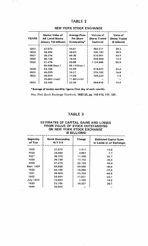
If we turn to capital gains and losses we encounter a surprisingproblem of measurement. A glance at the financial pages of anymajor newspaper indicates that the nation’s stock exchanges areprobably the most intensely monitored sector of the entire economy.Yet for all the data on the fluctuations in the prices of individualstocks or of price indices, there is little information on aggregatevalues. We do have monthly figures on the total value of outstandingshares on the New York Stock Exchange (see Table 2). In principle,several adjustments should be made in these numbers in order toobtain a measure of the capital gains and losses experienced byAmerican households. We should correct for new stock issues and
CHANGE OF STOCK PRICES GREEN 193
retirements, and more important, for the portion of these listedstocks which are owned by corporations or foreigners.4
We sometimes forget that the New York Stock Exchange was onlyone of 34 exchanges operating in this country in the 1920’s. Wereally want to know the capital gains and losses from all corporatestocks traded on all these exchanges (and even those traded privatelyperhaps). The only clue we have as to the relative importance of thenation’s largest exchange is the fact that on July 31, 1933, the valueof outstanding stock on the NYSE ($32.762 billion) represented34.5 percent of the total for all 34 exchanges.~
If we boldly assumed that {1) the relative size of the NYSE andother exchanges remained constant, and (2) prices on all the ex-changes always moved parallel to those on the NYSE, we could getone rough estimate of aggregate gains and losses to households bydoubling the shifts in value shown in the NYSE data.6 The results areshown in Table 3.
Capital Gains and Losses
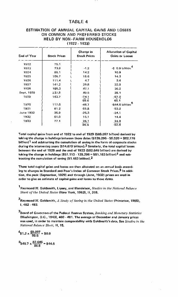
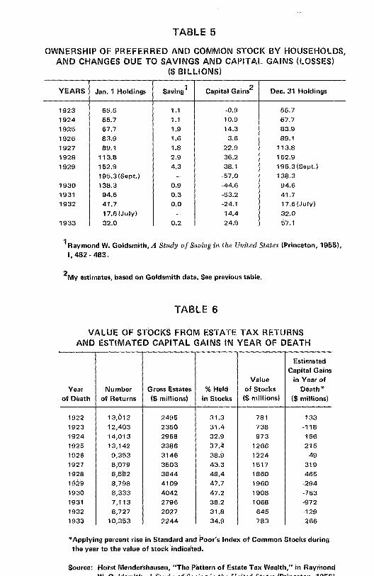
A second approach relies upon Goldsmith’s estimates of nationalwealth for 1922, 1929, and 1933, plus his annual estimates of house-hold saving through purchases of corporate stock. The capital gainsand losses (differences in holdings on balance sheet dates, lesscumulated saving during the interval) are allocated annually accord-ing to changes in an index of common stock prices. This morecomplicated procedure is presumably superior because it reflectschanges in stocks outstanding (e.g., new issues) and in the proportionheld by households. The results are shown in Tables 4 and 5. Thefairly close conformance of the two procedures is also reassuring.
4Goldsmith’s data indicate that at the end of 1922 households held 73 percent of thecorporate stock appearing on the national balance sheet. At the end of 1929 they still held74 percent, but by the end of 1933 their share had fallen to 56 percent (while the share otnon-financial corporations had risen sharply). See Raymond W. Goldsmith~ Robert E.Lipsey, and M. Mendelson, Studies in the National Balance Sheet of the United States (NewYork, 1963), II, 319.
5Senate Committee on BanMng and Currency, Report on "Stock Exchange Practices,’pp. 8-9.
6This would involve inflating the NYSE data by 1/34.5 to include other stock exchangesand deflating by .74 to reflect the share of outstanding stock held by households (see note zabove). No correction has been made for new issues or stock retirements.
194 CONSUMER SPENDING and MONETARY POLICY: THE LINKAGES
Obviously households experienced very large "paper" gains andlosses on corporate stocks in the market boom and bust of 1927-33.But how many of these paper gains and losses were actually "real-ized" through sales? We can get some indication from the gains andlo~ses recorded on income tax returns. The data, from a very carefulstudy by Lawrence Seltzer, are given in Table 7. The IRS source datacontain some biases of course. Taxpayers presumably under-reporttheir capital gains and exaggerate their losses. Prior to 1928 personswith net deficits in their statutory income were not required to filereturns (this probably meant primarily an under-reporting of capitallosses, which offsets the above biases). The most serious downwardbias arises from the exclusion of capital gains upon property trans-ferred ("realized"?) at death; we must look to estate tax records toadjust for this omission. The second limitation in the data is thatthey cover gains and losses upon all property, not just corporatestocks. Detailed data for 1936 reveal that 79 percent of realizedcapital gains and 68 percent of losses arose from corporate stocksand bonds. Thus, by using Seltzer’s original data for all gains andlosses we can surely offset any downward bias due to under-reporting.7
In order to estimate capital gains "realized" at death we look to astudy of estate tax data by Horst Mendershausen (see-Table 6). Thehigh tax exemption on estates means that we have data only on thewealthiest 1 percent of those dying in each year, persons with grossestates of over $100,000. But the ownership of corporate stock isheavily concentrated in the upper income groups, so we have prob-ably captured a substantial portion of the gains and losses from suchstock.S The gains or losses "realized" during the year of death are
7Lawrence H. Seltzer, The Nature and Tax Treatment of Capital Gains and Losses(NBER, New York, 1951), pp. 110-112, 145.
8Horst Mendershausen, "The Pattern of Estate Tax Wealth," in Raymond W. Goldsmith,A Study of Saving in the United States (Princeton, 1956), III, 287, 324-326. Let us make anillustrative calculation of the corporate stocks held by decedents with estates of less than$100,000. About one million adults died in 1929. Assume an average estate of $20,000, ofwhich 10 percent was held in corporate stocks (these should both be very generous esti-mates). Then the bottom 99 percent of decedents owned $2 billion of stock, just matchingthe holdings of the wealthiest 1 percent.
Obviously not all stocks transferred at death were actually sold at the time by the heirs.But since we are seeking an upward biased estimate of "realized" capital gains and losses, weinclude the full amount of these estate transfers in our final estimate. This procedure easilycompensates for the omission of the untaxed estates, as noted above.
CHANGE OF STOCK PRICES GREEN 195
estimated very roughly from the percentage rise or fall in an index ofstock prices. These figures are then added to Seltzer’s to provide anupward-biased estimate of total realized capital gains and losses (seeTable 7).
Impact of Capital Gains or Losses on Consumer Spending
Having estimated both the paper and realized capital gains andlosses in the stock market, we now come to the really tough empir-ical question. How much impact did they have upon the consumerspending of American households?
Ando and Modigliani, in their study of the "life cycle" savinghypothesis, have estimated that the marginal propensity to consumeout of net worth is about .06. That is, for each dollar of his networth a consumer will increase his spending by six cents. This coeffi-cient is generated from annual time series data for 1929-59, and isgenerally confirmed in Ando’s estimates for 1900-28; hence it seemsreasonable to apply it to the years around 1929. John Arena hasestimated a similar function which, however, includes a separate termfor the capital gains on net worth during each year. He derives (frompost~war data) an MPC on these capital gains of about .0.3, but hecannot confirm statistically a significant difference between thiscapital gains coefficient and his estimate of the broader Ando-Modigliani coefficient for net worth.9
If we apply the Ando-Modigliani coefficient to the total papercapital gains and losses in. the stock market,1° the implied shifts in
9Albert Ando and Franco Modigliani, "The ’Life Cycle’ Hypothesis of Saving: AggregateImplications and Tests," American Economic Review, LIII (1963), 55-84, and corrections inLIV (1964), 112-113. John J. Arena, "Capital Gains and the ’Life Cycle’ Hypothesis ofSaving," American Economic Review, LIV (1964), 107-111. In more recent estimates usingthe MIT-FRB econometric model, Ando and Modigliani have derived a coefficient of .04;see Frank deLeeuw and Edward Gramlich, "The Channels of Monetary Policy," FederalReserve Bulletin, (June, 1969), p. 481. I can think of several arguments f6r questioning thestability of this parameter during the extraordinary years of stock market boom and crash,but they are not unambiguous enough to suggest an alternative estimate.
10Strictly speaking we should be deducting from capital gains (or losses) any changes inhousehold borrowing to finance stock purchases, in order to arrive at changes in net worth.Brokers’ loans, bank loans, and other loans on securities were large in the boom of 1928-29,probably reaching a peak of $18 billion in September, 1929. But the year-to-year change insuch loans, which is the relevant statistic for changes in net worth, never exceeded about $3billion. Such small amounts would not significantly affect our estimates. See ShawLivermore, "Loans on Securities, 1921-32," Review of Economic Statistics, XIV (1932),191-194, and Goldsmith, A Study of Saving, I, 710.
196 CONSUMER SPENDING and MONETARY POLICY: THE LINKAGES
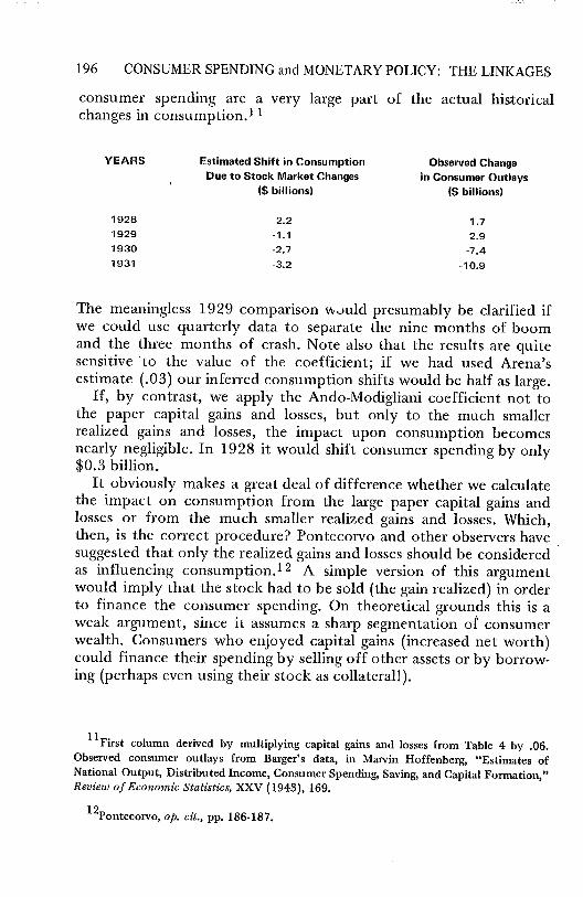
consumer spending are a very large part of the actual historicalchanges in consumption.1 1
YEARS Estimated Shift in ConsumptionDue to Stock Market Changes
The meaningless 1929 comparison would presumably be clarified ifwe could use quarterly data to separate the nine months of boomand the three months of crash. Note also that the results are quitesensitive ’to the value of the coefficient; if we had used Arena’sestimate (.03) our inferred consumption shifts would be half as large.
If, by contrast, we apply the Ando-Modigliani coefficient not tothe paper capital gains and losses, but only to the much smallerrealized gains and losses, the impact upon consumption becomesnearly negligible. In 1928 it would shift consumer spending by only$0.3 billion.
It obviously makes a great deal of difference whether we calculatethe impact on consumption from the large paper capital gains andlosses or from the much smaller realized gains and losses. Which,then, is the correct procedure? Pontecorvo and other observers havesuggested that only the realized gains and losses should be consideredas influencing consumption.12 A simple version of this argumentwould imply that the stock had to be sold (the gain realized) in orderto finance the consumer spending. On theoretical grounds this is aweak argument, since it assumes a sharp segmentation of consumerwealth. Consumers who enjoyed capital gains (increased net worth)could finance their spending by selling off other assets or by borrow-ing (perhaps even using their stock as collateral!).
llFirst column derived by multiplying capital gains and losses from Table 4 by .06.Observed consumer outlays from Barger’s data, in Marvin Hoffenberg, "Estimates ofNational Output, Distributed Income, Consumer Spending, Saving, and Capital Formation,"Review of Economic Statistics, XXV (1943), 169.
12pontecop¢o, op. cir., pp. 186-187.
CHANGE OF STOCK PRICES GREEN
Impact on Consumption OverestimatedThrough Use of Paper Capital Gains and Losses
197
Theoretically, then, the larger paper gains and losses seem to bethe appropriate variable by which to estimate changes in consumerspending. Despite the theoretical appeal of the larger estimates, thereare three arguments which lead me to conclude that they substan-tially overestimate the market’s impact upon consumer spending.First, persumably consumers normally respond to shifts in stockprices only imperfectly, and with some lag in recognition and adjust-ment. Spending decisions are not based on day-to-day or evenmonth-to-month fluctuations in net worth, but upon some subjectiveperception of more "permanent" changes. To approximate suchresponses we might appropriately "smooth out" some of the sharpestfluctuations in stock prices. Many households obviously held stocksright through the sharp peak in the market in September, 1929,without adjusting their spending either to their temporary capitalgains or to the counterbalancing paper losses after the crash, la
Secondly, the unusually low ratio of realized to paper gains andlosses during the boom and crisis years of 1927-31 may be thesymptom of a short-term downward shift in the Ando-ModiglianiMPC out of net worth. Perhaps individuals decreased their propensityto spend out of capital gains in order to retain more of their wealthin the rising market. On the other hand, the capital losses after thecrash, and the resulting illiquidity and danger of bankruptcy, mayhave temporarily raised the MPC coefficient for net worth, compel-ling consumers to make unusually large reductions in their spendingfor given reductions in their wealth.
A third piece of evidence strengthens my inclination to conside~the estimated shifts of consumption based upon paper gains andlosses as an upper limit value. Nancy Dorfman has run a regression otper capita real consumption upon Milton Friedman’s estimates otpermanent income per capita, for the years 1919 to 1938. The-crucial years 1927 to 1930 all fall perfectly on the regression lineThere are no large residuals to show an effect of capital gains (nocounted in permanent income) upon consumption.14
13Our use of annual data (and omission of the strong peak during 1929) is one crude wa~of "smoothing" our capital gains data.
14Nancy S. Dorflnan, "The Role of Money in the Investment Boom of the Twenties anthe 1929 Turning Point" (unpublished Ph.D. dissertation, University of California, Berkele51967), pp. 170-172. Admittedly a better test would be to look at residuals in thAndo-Mocligliani consumption function.
!98 CONSUMER SPENDING and MONETARY POLICY: THE LINKAGES
Although the aggregate data leave considerable leeway for doubt, Ia~n presently inclined to conclude that capital gains and losses in thestock market during 1927 to 1931 caused shifts in aggregate con-sumer spending of less than $1 billion per year.
Concentration of Stoch Ownership
Another line of research may eventually help to reduce the rangeof uncertainty about the impact of the market upon aggregate con-sumer spending. We can move toward the microeconomic level ofanalysis.Rhetoric in the 1920’s, often repeated uncritically byhistorians, spoke of stock market speculation as a popular pastimefor the masses. Housewife, shoe-shine boy, and laborer supposedlyjoined the businessman and the Wall Street "insider" to seek theirfortunes. Yet all the responsible estimates clearly show that only asmall minority (8 percent) of the population actually owned stock,and that within this minority the substantial holdings were heavilyconcentrated in the hands of the wealthy few, with 500,000 to600,000 individuals owning between 75 and 85 percent of the out-standing stock.15
Given this heavy concentration of stock ownership, we should notexpect to observe much direct impact (via capital gains and losses)upon the purchases of mass consumption items. Rather the effectson spending should be concentrated in luxury consumer goods andservices, and in consumer durables. Ideally we should undertakemultivariate analysis of these consumer purchase categories to sortout the particular influence of the stock market. We must settleinstead for a glance at the gross output data. The available evidencegives only selective and weak support to our hypothesis of largeimpacts. Automobile sales did reach record levels in the spring of1929 and fell off dramatically in November; between 1929 and 1930the reduction in this one item was over $1 billion. But how much ofthis decline was caused by capital losses in the stock market? Othermonthly data on luxury consumer spending--such as railroad pas-senger mileage, foreign travel, hotel occupancies, or visits to National
15Alfred L. Bernheim, et al, The Security Markets (New York, The Twentieth CenturyFund, 1935), chapter Ill and Appendix I. The number of stockholders apparently didincrease sharply duYing the boom years, probably between 50 and 100 percent. The totalnumber of stockholders reached approximately ten million individuals in 1930, but thepercentage of value held by the highest income groups increased even during these years ofspreading ownership.
CHANGE OF STOCK PRICES GREEN 199
Parks--adhere closely to seasonal and trend values, reflecting novisible response to the boom or crash. 16
II. Effect on Capital Spending
The second hypothesis is: Low yields on stocks and the easy speculative atmo-sphere of the boom market stimulated corporations to finace expanded real in-vestment spending through new stock issues. After the crash, higher yields and amore restrictive market caused a contraction of real investment spending.
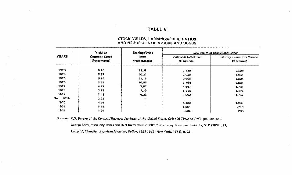
It is true that the average yield on common stocks (the ratio ofdividends to prices) fell substantially during the 1920’s from nearly 6percent in 1923 to under 3 percent at the peak of the boom inSeptember, 1929 (see Table 8). At the peak of the boom, yields oncommon stocks were well below those on less risky corporate andgovernment bonds. 17
But falling current yields or earnings/price ratios did not neces-sarily make stocks a cheap form of financing. If a businessmanbelieved that the market price of his company’s stock accuratelyreflected the potential growth of its future earnings, he would notconsider a low current yield ratio "cheap"; his opportunity cost offinancing would consider those higher future earnings. On the otherhand, if stock buyers were bidding yields down in anticipation ofspeculative capital gains from the stock market, rather than capitalgains from future company performance in the real economy, thenbusinessmen might consider stock prices "unrealistically" high, andperceive the yields as "cheap.’’18
The temporary bulge in stock issues in 1928-29 suggests that manybusinessmen did consider them a financing bargain. The data col-lected by the Commercial and Financial Chronicle on issues ofcorporate stocks and bonds for "new capital" show a dramatic in-crease during the decade, and a sharp decline after the crash (seeTable 8). Raymond Goldsmith’s data show that new issues of stocks
16U.S. Bureau of the Census, Historical Statistics of the United States, Colonial Times to1957 (Washington, D.C., 1960), p. 462. Survey of Current Business, Annual Supplement,1932, pp. 9, 119-123, 273-275.
17Historical Statistics, pp. 656, 658 (See Table 8.) Yontecorvo, op. cit., pp. 178-179.Robert Sobel’s claim that price]earnings ratios were not abnormally high in the boom isquite misleading; he gives fragmentary data rather than the more comprehensive averages,and for 1928 rather than 1929. See Sobel, op. cir., pp. 119-122.
18Dorfman, op. cir., chapter VII.
200 CONSUMER SPENDING and MONETARY POLICY: THE LINKAGES
and bonds provided about one-third of total corporate sources offunds (1923-29), making them second in importance to internalsources (55 percent) such as retained earnings and depreciationallowances. Stocks alone provided about 19 percent of total financialsources; this was a much higher percentage than Goldsmith observedfor other years of the 20th century. These statistics certainly lendapparent support to the hypothesis that easy financing via corporatestocks stimulated real investment spending. 19
Appearances can be deceptive! A further examination of thesestatistics will cause us to reject the hypothesis. The basic source ofconfusion is the failure to distinguish between financial capital andphysical capital. The term "new capital" as used in the FinancialChronicle refers to financial capital, to those issues not used forrefunding or retirement of old securities. Many of these "newcapital" issues provided funds for corporate mergers or acquisitions,or for financial "working capital." We want to know how much ofthis new financial capital actually paid for new physical capital, plantand equipment or inventories.
A series published by Moody’s Investors Service of new securityissues for "productive purposes" (see Table 8) gives us a goodmeasure of such real capital formation, although it excludes inven-tory accumulation and involves some rough estimation. The data givestriking refutation to our hypothesis. While new issues of stocks andbonds were rising dramatically from $2.6 billion to $8 billion, theamount going to finance real investment remained virtually constant,between $1.5 and $2 billion per year. Betv~een 1921 and 1929 newissues financed only about 26 percent of corporate gross investment,at a steady pace apparently little affected by the stock marketboom. 2o
A very thorough study by George Eddy of "Security Issues andReal Investment in 1929" provided decMve and more detailedevidence for that climatic year of the boom. After carefully tracingthe ultimate use made by each corporation of its share of the $8.002
19Raymond W. Goldsmith, Financial Intermediaries in the American Economy since1900 (Princeton, 1958), pp. 222-223.
2,~Ge.orgen Eddy, "Security Issues and Real Investment in 1929," Review of EconomicStatistics, XIX (1937), 90-91. Dorfman, op. cir., p. 108. The division of new issues betweenstocks and bonds was strongly influenced by yields and expectations (Pontecorvo, op. cit.,pp. 176-179). But we cannot infer from this fact how stocks and bonds shared the financingof real investment. Eddy’s data for 1929 show that the stock issues went disproportionatelyto mergers and other financial purposes, while the bond issues went disproportionately toreal investment.
CHANGE OF STOCK PRICES GREEN 201
billion of new issues listed in the Financial Chronicle, Eddy con-cluded that only $2.002 billion financed real investment spending.Common and preferred stock accounted for 74 percent of the $8billion of new issues, but only 54 percent ($1.074 billion) of the $2billion of real investment. Thus the booming stock market of 1929directly financed only $1.1 billion out of $17.2 billion of grossprivate investment. 21
What about the second part of our hypothesis, the impact of thecrash upon stock financing of real investment? Moody’s series of"productive" new issues reached its peak in 1930 (not 1929!) but weknow that this was due mainly to large new bond issues, especiallyby public utilities. Stock yields rose sharply as prices collapsed, andafter mid-1930 new issues slowed to a trickle. But even if we assumethat new issues of stock financed no real investment at all after 1929,this could only have caused a reduction of $1.1 billion in annual realinvestment spending. If we believe that the real economic declinewhich began in mid-1929 had its major causes outside the stockmarket, then we would expect some decline in externally financedreal investment even without the crash. External finance is alwaysmost important in an expanding economy, while internal finance(liquidity, cash flows from retained earnings) matters more inrecession.22
In summary, the stock market boom induced a flood of newcorporate stock issues, some substituting for bonds or other secu-rities and some doubtless representing net financial expansion whichwould not otherwise have occured. But the volume of real physicalinvestment financed directly by new stock issues remained constantand apparently unaffected by the market boom. The stock marketcrash probably reduced real investment by much less than $1 billionper year, with the main impact largely offset in 1930 because ofshifts back to bond issues.
21Eddy, op. cir., pp. 79-86. Hoffenberg, op. cir., p. 169. See below, pp. 21-22, for briefdiscussion of indirect uses of those funds.
22This is the "bifurcation hypothesis" of investment theory. See Michael FL Evans,Macroeconomic Activity: Theory, Forecasting, and Control (New York, 1969), pp. 90-92,128-129.
202 CONSUMER SPENDING and MONETARY POLICY: THE LINKAGES
IlL Psychological Impact on Consumption
The third hypothesis is: The stock market boom of 1928-29 improved consumerand business expectations, confidence, and optimism, and thus raised consump-tion and investment spending. The crash brought lower expectations and pes-simism, and therefore lowered spending.
Casual assertion of the great psychological impacts of the stockmarket boom and crash pervades the literature. Perhaps its popular-ity is directly related to the difficulty of proving or disproving it. ifall other casual connections between the market and the economyhave been found wanting, one can always fall back upon thepsychological impact. I will attempt to demonstrate the severe limita-tions of the assertion by showing its conceptual weakness and byindicating the direct and indirect evidence against its importance.
All decisions are based upon "expectations." Behavioral theoriesin the social sciences, and particularly those in economics, do notignore or deny the role of expectations or psychology in decisions.Rather, they assume that these inner psychological states are usually(and on the average) related in some stable, predictable fashion toobservable, "objective" conditions in the decision maker’s environ-ment. Most businessmen, for example, make their decisions aboutreal investment spending with "psychological expectations" that arestrongly influenced by such "objective" data as income, sales, capac-ity utilization, interest rates (or stock prices!), prices vs. costs, etc.
We do not enhance our explanatory powers, then, if we refuse toprobe beneath such vague and all-embracing terms as "confidence"or "expectations" to the underlying objective conditions. Instead weshould construct behavioral models in which we spell out more pre-cisely and explicity just how we believe the decision making actorsrespond to given information and situations. Perhaps they will extra-polate (or "forecast") the present level of prices or costs or profitsinto the future. Or perhaps they will usually "expect" some rate ofincrease or decrease from present levels. Once we have specified these"normal" responses we can speak more meaningfully, and more nar-rowly, of a "shift in expectations," as referring to some change in theresponse parameters.
How does this conception apply to our discussion of the stockmarket? It means that much of the shift from "optimism" and "con-fidence" in 1928 or 1929 to "pessimism" and "a mood of hesita-tion" in 1930 or 1931 represented merely a normal, predictableresponse to changes in objective conditions--declining GNP, falling
CHANGE OF STOCK PRICES GREEN 203
profits, rising unemployment. We should then rephrase our hypoth-esis to ask whether there was some additional "subjective" shift ofexpectations, some alternation of the "normal response" of decisionmakers to these changing objective conditions, and whether any suchshift was related to the stock market.
What sort of direct evidence do we have regarding the influence ofthe stock market upon the "optimism" or "pessimism" ofAmericans, or the influence of those attitudes upon spending de-cisions? The evidence is overwhelming that "expectations" about thefuture of the stock market itself shifted upward in 1928 or 1929;masses of buyers began betting upon a rising market. Similarly, theevidence of "panic" psychology in the market in October andNovember, 1929, is undeniable. There is also much testimony tosuggest that these states of "confidence" or "panic" among buyersand sellers of stocks were influenced by the perception of changingconditions in the real economy. For example, the belief in a "newera" of "permanent prosperity" surely influenced the way manypeople capitalized current corporate earnings in 1929.
The state of expectations in the stock market in December, 1929,and the first half of 1930 is more ambiguous. Certainly the mood ofpanic had receded. Stock prices stabilized and even recovered someof their lost ground, and most observers suggested a feeling of mildoptimism about the future of the market.
But our chief purpose is not to describe the shifting "expecta-tions" about the stock market itself, nor to explain those shifts interms of changes in the real economy. We seek some evidence thatthe changing expectations in the market "carried over" and influ-enced expectations about spending on real output, consumption andinvestment. At this crucial juncture there is remarkably little sup-porting evidence for the hypothesis. Where are the people saying,"The stock market boom has so raised my optimism [though not myincome or wealth!] that I am going to buy a car, or add a wing to myfactory"?
In the midst of the crashing market on Black Thursday (October24, 1929) President Hoover issued a statement that "the funda-mental business of the country--that is, the production and distribu-tion of goods and services--is on a sound and prosperous basis."Similar statements were issued by economists, businessmen, andnewspaper editors over the next several months. Historians, likeMonday morning quarterbacks, have cited these statements as ex-amples of poor forecasting or empty rhetoric. Let us admit thatHoover’s statement was a bad forecast, and even a bad description of
204 CONSUMER SPENDING and MONETARY POLICY: THE LINKAGES
the present state of the economy at the time. It is still a strikingpiece of evidence against our expectations hypothesis. Hoover istrying to reassure the "panicky" speculators. He assumes that thereal economy influences expectations in the stock market, not theother way around! The frequent repetition of such optimistic com-mentary in early 1930 strongly suggests that "pessimism" and"panic" in the stock market did not immediately cause a sharpadverse shift in expectations about the real economy.23
Let us turn now to the indirect evidence on the expectationshypothesis. Assume that there was a substantial subjective increase in"optimism" in 1928-29, beyond any changes in "objective" eco-nomic conditions, or that there was a substantial "pessimistic" shiftin subjective expectations after the crash. If these altered attitudesaffected spending decisions, we would then expect to find large"unexplained residuals" in our consumption or investment functions.The actual spending should be substantially higher in 1928-29 andsubstantially lower in 1930-31 than we would "predict" (estimate)from an econometric model which assumes stable, "normal" re-sponses to changes in the objective variables. 24
I have examined a number of plausible models for consumer andinvestment spending which have been fitted to data from theAmerican economy in the inter-war years (e.g. 1920-1941). None ofthem show the sort of large residuals for the years 1928-31 whichwould support our hypothesis of subjective shifts toward"optimism" and "pessimism." In Nancy Dorfman’s regression of percapita real consumption on per capita real consumption on per capita
23Sobel, The Great Bull Market, pp. 137-146. Hoover’s quotation is on p, 137.
24It is not necessary to believe that our econometric model is perfectly correct in itsspecification for this approach to be useful. It is enough that our excluded variable (the shiftin expectations) be uncorrelated with the included variables, such as permanent income,profits, or past physical capital. If the correlation were high, movements of ’the includedvariables would "pick up" and "mask" much of the influence of our expectations variable,leaving no residuals. I would argue that stock market expectations depend mainly uponcapital gains and losses. These capital gains are not included in measured income or profitsand their statistical correlation appears to be fairly low (I have not tested this rigorously.).If, however, stock market expectations are strongly influenced by the performance of thereal economy (as well as by market performance), this correlation will undermine myprocedure. Many economists do assume that in general the stock market is a fairly good"barometer" or "leading indicator" whose movements reflect or anticipate (i.e., correlatewith) swings in the real economy; But the historical discussions also emphasize that anysuch correlation broke down during 1928-30, when the market was "over-optimistic"relative to the real economy.
CHANGE OF STOCK PRICES GREEN 205
permanent income, the years 1927-31 fall right on the line. InLawrence Klein’s econometric model (I) real investment is a functionof past and current profits and the initial stock of physical capital.His regression does show actual investment in 1929 which is $1.1billion above the estimated investment level. But the Moody’s invest-ment series and George Eddy’s careful study of the stock issues andreal investment in 1929 seem to close that loophole. Klein’s moredetailed model (III) of plant and equipment investment (as afunction of current and lagged output and initial capital stock) hasno residuals over $750 million. These results seem to leave fairlylittle empirical maneuvering room for any massive expectationseffects upon aggregate spending. 25
IV. Impact on Banks
Our fourth hypothesis is: The crash threatened the liquidity and solvency offinancial intermediaries, especially investment trusts, holding companies, andcommercial banks. Their iiliquidiW or failure restricted credit flows or tied up ordestroyed liquid assets which were essential td consumers and businesses.
Galbraith has argued that the investment trusts and holdingcompanies caused a reduction of real investment spending. Theyfought to sustain the dividends of the operating companies whichthey controlled, since these dividends were their vital source ofincome and liquidity in a falling stock market. High dividends at atime of tumbling profits meant a sharp drop in retained earningswhich could finance real capital formation. 26
This argument is logical enough, but the effect in 1929 must havebeen quantitatively insignificant. The total assets of investment com-panies and investment holding companies reached a peak of $7.4billion in 1929 and declined to $3 billion by 1933. Compare this tocommercial bank assets of $66 billion, or to the value of stock on theNew York exchange alone of $65 billion. These investment com-panies owned only 3.6 percent of outstanding corporate stock, and
25Dorfman, op. cit., pp. 170-172. Lawrence R. Klein, Economic Fluctuations in theUnited States, 1921-194.1 (New York, 1950), pp. 68-69, 102-114.
26Galbraith, The Great Crash, p. 183. Galbmith implies that investment holding com-panies were sharply different fi’om other corporations in their deterraination to sustaindividends during recession. But John Lintner has shown that dividends for all corporationsbehave this way. This puts the burden of proof more heavily upon Galbraith, since only thedifferential behavior of investment holding companies would support his argument. See.Lintner, "The Determinants of Corporate Savings," in Walter W. Heller, et al (eds.), Savingsin the Modern Economy (Minneapolis, 1953), pp. 248-253.
206 CONSUMER SPENDING and MONETARY POLICY: THE LINKAGES
thus controlled about that share of corporate dividends. Even ifevery single dollar of corporate dividends which they received hadbeen retained and had been spent on real investment, only about$225 million of added investment would have occured (3.6 percentof the $6.3 billion of corporate dividends). 27
There is virtually no evidence to support the popular impressionthat the suspension and failure of commercial banks after 1929 wasthe result of their prior involvement in financing stock market"speculation." It is easy to tell colorful stories about Charlie Mitchelland his National City Company, the highly promotional and hardselling investment banking affiliate of the National City Bank of NewYork (of which Mitchell was also president). It is mt~ch more dif-ficult to show that the success or failure of such affiliates (did manyfail?) affected the solvency of the commercial banks. 28
The waves of bank failures began not right after the stock marketcrash, but after October, 1930, and again in 1931 after the inter-national monetary crisis. The heaviest losses were suffered not onstocks but on real estate and business loans, and on government andcorporate bonds. Bank failures came not to Wall Street, where thestock market credit was concentrated, but to small independentcountry banks and to banks in communities which had suffered theheaviest losses of income and employment in the depression.29
Commercial banks owned only 0.8 percent of the outstandingcorporate stock in 1929, a total of $1.2 billion. Of course their reallysignificant involvement in Wall Street came through "loans onsecurities" to brokers and dealers or to individual speculators. Theseloans "for purchasing or carrying securities" reached $8.3 billion in1929, compared to toal commercial bank assets of $66 billion. Thus
27Raymond-- W. Goldsmith, The Share of Financial Intermediaries in National Wealth andNational Assets, 1900-1949 (New York, 1954), pp. 68-71. Goldsmith, Financial Inter-mediaries in the American Economy since 1900, pp. 73-74. Some investment (especiallyholding) companies used financial "leverage" of course, controlling (but not receiving) all ofthe dividends of a company while owning 51 percent (or often less) of its stock. As an offsetagainst this, they oftened owned shaxes of stock in companies whose dividend policies theydid not control. I have assumed for convenience that these effect roughly cancelled.
28patterson, The Great Boom and Panic, pp. 50-52. I have not investigated in any detailthe possible linkages exposed by the Congressional Hearings of 1932-34 on "Stock Ex-change Practices."
29Lester V. Chandler, America’s Greatest Depression, 1929-1941 (New York, 1970), pp.77-84. Milton Friedman and Anna Schwartz, A Monetary History of the United States,1867-1960 (Princeton, 1963), chapter 7.
CHANGE OF STOCK PRICES GREEN 207
if all these loans had defaulted after the crash, the losses would haverepresented 13 percent of bank assets. In fact, however, bankerssuffered very little loss on such loans. The risks and losses were borneby the borrowers, and the banker could easily check on a daily basisto assure himself that the security collateral was sufficient to coverthe loan. 3o
V. Impact on Credit
Our fifth hypothesis is: Stock market speculation absorbed credit funds, divertingthem away from financial real investment (or consumer) spending. After the crashthe release of funds from speculation made money and credit more available tofinance real spending.
This argument, as stated above, still has several points of confusionor ambiguity imbedded in it. Does it refer to all credit, to bankcredit, or to money? Does it assume some sort of fixed, limited"pool of funds," where increased allocations to one user (the stockmarket) automatically mean decreased allocations to others? Withthese problems in mind we shall consider several versions or varia-tions of the original hypothesis.
In one important mechanical sense, stock market transactionscannot "absorb" funds: for every buyer of stock who gives up fundsthere is a seller who receives them! Dollars going "into the market"do not disappear, but "come out the other side." Even if the firstseller uses his funds to buy other stocks, eventually some sellerremoves his funds from the market. From this perspective, then, onemight in principle measure the impact of market trans~ictions uponthe real economy by comparing what stock sellers actually do withtheir funds to what buyers would have done with their funds if theyhad not bought stocks. The alternatives for both groups obviouslyinclude: buying current output (either consumption or investment);buying existing physical capital; buying other stocks (outstanding, ornew issues); buying bonds, mortgages or other financial assets; re-tiring old debts or securities; "hoarding" bank deposits or currency.
In practice this formulation does not seem to lend itself toempirical verification. It does suggest one specific inquiry, however.What happened to the billions of dollars raised by new issues of
30Goldsmith, Financial Intermediaries in the American Economy since 1900, p. 225.Goldsmith, A Study of Saving, I, 710. Charles O. Hardy, Credit Policies of the FederalReserve System (Washington, D.C., 1932), p. 174.
208 CONSUMER SPENDING and MONETARY POLICY: THE LINKAGES
corporate stocks which were not used to finance real investmentspending? If they went to financing mergers or acquisitions, what didthe recipient companies or individuals do with the funds?
If they were re-lent into the call loan market, where did theyeventually flow into real expenditures? Further study of the financialstatements of the issuing corporations (along the lines of Eddy’sstudy) might at least permit us to identify the first links in thesechains of transactions. It appears likely that in the late 1920’s mostof the financial capital from new issues went to mergers and acquisi-tions. Perhaps as muchas $3 billion of corporate funds (including theexcess cash balances of many corporations not issuing new stocks)went into brokers’ loans. 31
Another fruitful perspective comes from the modern theory of"balancing portfolios." Imagine that all holders of wealth--individuals, corporations, financial intermediaries, etc.--desire to holdsome mixture of assets: physical capital, consumer durables, stocks,bonds, mortgages, insurance policies, money, or other financialassets. A strong speculative boom which attracts investors to thestock market will thus reduce their demands for other assets in theirportfolios. Lower bond and mortgage prices mean higher interestrates. Lower prices on existing physical capital mean a lower profiton investment in new physical capital. While lower yields and higherprices on stocks would stimulate real investment by stock-issuingcorporations (our second hypothesis above), the higher cost offinancing (and perhaps lower profit expectations) would reducethose types of real investment customarily financed by bonds ormortgates. Thus while directly or indirectly raising real investmentthrough stock issues, the stock market boom also indirectly de-pressed it elsewhere in the economy. Conversely, the market crashshifted asset demands back toward bonds and mortgages, andencouraged real investment activities which they financed. Unfor-tunately, I have not yet figured out a way of testing or quantifyingthe implication of this "portfolio balancing" theory.
Perhaps the most controversial version of this fifth hypothesisfocuses narrowly on bank credit. Did the "speculative" stock marketboom "absorb" bank credit or "tie up" bank deposits, leaving lesscredit and money available to meet the "legitimate" needs ofindustry, agriculture, and commerce? The Federal Reserve leadersused this argument to justify their restrictive monetary policy actions
31Board of Governors of the Federal Reserve System, Banking and Monetary Statistics(Washington, D.C., 1943), pp. 497-498.
CHANGE OF STOCK PRICES GREEN 209
in 1928 and 1929. The issue was vigorously debated among mone-tary economists through the early 1930’s. After examining thisdebate, and gathering some relevant statistics, I have come to thefollowing conclusions.
1. Loans by banks to stock exchange brokers and dealers did notkeep billions of dollars "tied up in financial circulation." The brokersmerely extended the chain of financial intermediation, channelingfunds through margin loans to corporations issuing new stocks or toindividuals selling old stocks. By these channels the real savings ofbank depositors soon flowed into some form of expenditure.32
2. During 1928 and 1929 virtually all the increase in brokers’ loanscame from non-bank sources (corporations, foreigners, wealthy indi-viduals). To the extent that brokers or their customers used theseoutside funds to repay debts to banks, bank credit was actuallyreleased for other uses. In the three months after the crash inOctober 1929, these non-bank lenders withdrew over $4 billion offunds from brokers’ loans. The banks were able to increase theirintermediation in this crisis, lending $1.3 billion to stock brokers andspeculators in the first week of the crash alone. This was done with-out a proportionate contraction of bank credit to other customers,because the Federal Reserve (especially the New York Bank) ex-panded bank reserves. 3~
3. Stock market transactions did not tie up large amounts of bankdeposits. Stock brokers could themselves handle a huge transactionsvolume by bookkeeping entries on their own books, or by nettingout daily balances among brokers. Because of this economizing oftheir deposit balances, brokers’ deposits-had an extremely high andelastic velocity of turnover. During the mid-1920’s brokers requiredonly about $20 million of deposit balances to conduct billions ofdollars of transactions! a 4
32Lauehlin Currie, "The Failure of Monetary Policy to IS"event the Depression of1929-32," Journal of Political Economy, XLII (1934), 145-177. John H. Williams, "TheMonetary Doctrines of J. M. Keynes," Quarterly Journal of Economics, XLV (1931),558-573. Harold Barger, "The Banks and the Stock Market," Journal of Political Economy,XLIII (1935), 763-777. Harold L. Reed, Federal Reserve Policy, 1921-1930 (New York,1930), chapter V. Hardy, op cir., pp. 148-172.
33Banking and Monetary Statistics, p. 494. Portecorvo, op cir., p. 181. Friedman andSchwartz, op. cit., p. 335.
34~ardy, op cir., p. 167,
210 CONSUMER SPENDING and MONETARY POLICY: THE LINKAGES
Of course the "speculators," the buyers and sellers of stocks, alsoutilized bank deposits, not only in New York but all around thecountry. But they too could conduct transactions through theirbrokers’ accounts rather than bank accounts, and could increase theaverage velocity of their deposits by lending in the call loanmarket. 85
The argument that the stock market "tied up" bank depositsimplies that there was only a fixed "pool of funds" available. With afixed total money supply (and fixed velocity!) more dollars circu-lating in the financial sector (the stock market) must mean fewerdollars available for transactions in the real sector. But this implicitassumption does not fit the facts in our case. Both the dollar volumeof stock market transactions and its rate of increase were smallcompared to the volume and rate of increase of bank debits, that isthe transactions volume in bank demand deposits (bank debits = MV= money supply multiplied by transactions velocity or annual turn-over). The $90 billion of shares traded on the New York StockExchange in 1929, even if each transaction had been conducted bycheck (rather than on brokers’ accounts), amounted to only 1~ per-cent of the $~9~ billion of debits in the reporting New York City
~banks. The estimated $225 billion of stock transactions on all ex-changes were 18 percent of bank debits ($12~7 billion) in all com-mercial banks. The $16.7 billion rise in stock transactions from 199-8to 1929 on the NYSE was only 16 percent as large as the ($102billion) rise in debits of New York City banks, while the rise in allexchanges ($42 billion) was 26 percent of the rise in debits of allcommercial banks. Most of this increase in bank debits came throughrising average velocity, and only a little through increased deposits.As noted above, the stock market exhibits a uniquely high trans-actions velocity for money.~6
35Ibid., p. 168.
36See Tables 2 and 9 for data in this paragraph. There are no available statistics on thedollar volume of stock exchange transactions, even for the New York Stock Exchange. Iconstructed the series in Table 2 by multiplying the number of shares traded by the averageprice of shaa-es outstandinD If we assume that lower priced shares trade more actively, thenthese figures may have a slight upward bias.
The NYSE data on shares traded do not include odd lot transactions (of less than 100shares}. Round lot transactions accounted for roughly 2/3 of total shares traded on theNYSE. In 1928-29 that exchange conducted about 60% of the share trading volume on allexchanges (U.S. Senate, Committee on Banking and Currency, 73 Cong., 2 sess., Hearings on"Stock Exchange Practices," Part 17, p. 7854}. Thus we can "inflate" the NYSE volume($90 x 3[2 x 10/6 = $225 billion) to obtain an estimate for trading volume on all exchanges.
CHANGE OF STOCK PRICES GREEN 211
Most versions of this fifth hypothesis have contained theoreticalflaws or have implicitly assumed institutional arrangements or condi-tions contrary to the historical facts. The "portfolio balancing"theory is logical enough, but it implies both upward and downwardshifts in different categories of spending, and it is not readily ame-"nable to quantitative estimation.
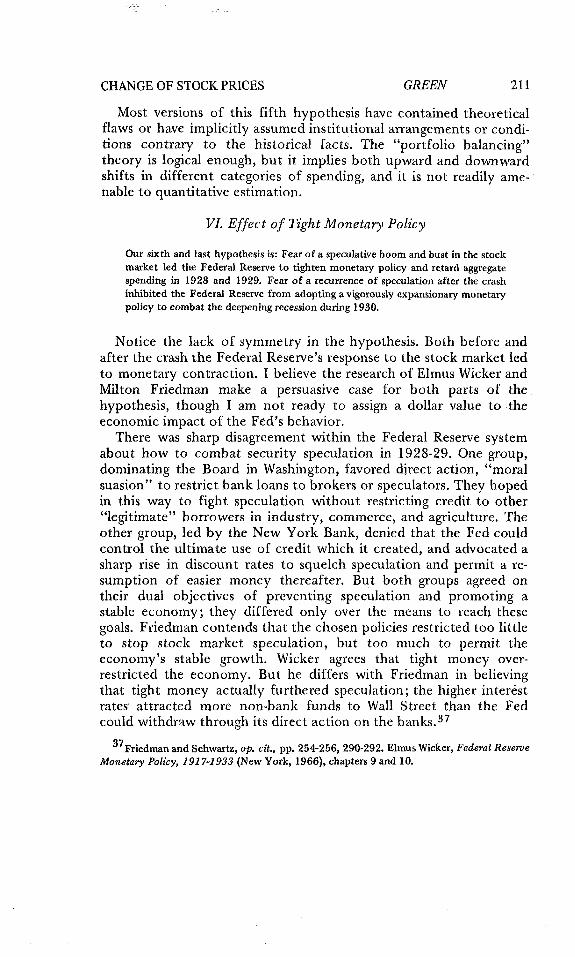
VI. Effect of Tight Monetary Policy
Our sixth and last hypothesis is: Fear of a speculative boom and bust in the stockmarket led the Federal Reserve to tighten monetary policy and re~ard aggregatespending in 1928 and 1929. Fear of a recurrence of speculation after the crashinhibited the Federal Reserve from adopting a vigorously expansionary monetarypolicy to combat the deepening recession during 1930.
Notice the lack of symmetry in the hypothesis. Both before andafter the crash the Federal Reserve’s response to the stock market ledto monetary contraction. I believe the research of Elmus Wicker andMilton Friedman make a persuasive case for both parts of thehypothesis, though I am not ready to assign a dollar value to theeconomic impact of the Fed’s behavior.
There was sharp disagreement within the Federal Reserve systemabout how to combat security speculation in 1928-29. One group,dominating the Board in Washington, favored direct action, "moralsuasion" to restrict bank loans to brokers or speculators. They hopedin this way to fight speculation without restricting credit to other"legitimate" borrowers in industry, commerce, and agriculture. Theother group, led by the New York Bank, denied that the Fed couldcontrol the ultimate use of credit which it created, and advocated asharp rise in discount rates to squelch speculation and permit a re-sumption of easier money thereafter. But both groups agreed ontheir dual objectives of preventing speculation and promoting astable economy; they differed only over the means to reach thesegoals. Friedman contends that the chosen policies restricted too littleto stop stock market speculation, but too much to permit theeconomy’s stable growth. Wicker agrees that tight money over-restricted the economy. But he differs with Friedman in believingthat tight money actually furthered speculation; the higher interfistrates attracted more non-bank funds to Wall Street than the Fedcould withdraw through its direct action on the banks.37
$TFriedman and Schwartz, op. cit., pp. 254-256, 290-292. Elmus Wicker, Federal ReserveMonetary Policy, 1917-1933 (New York, 1966), chapters 9 and 10.
212 CONSUMER SPENDING and MONETARY POLICY: THE LINKAGES
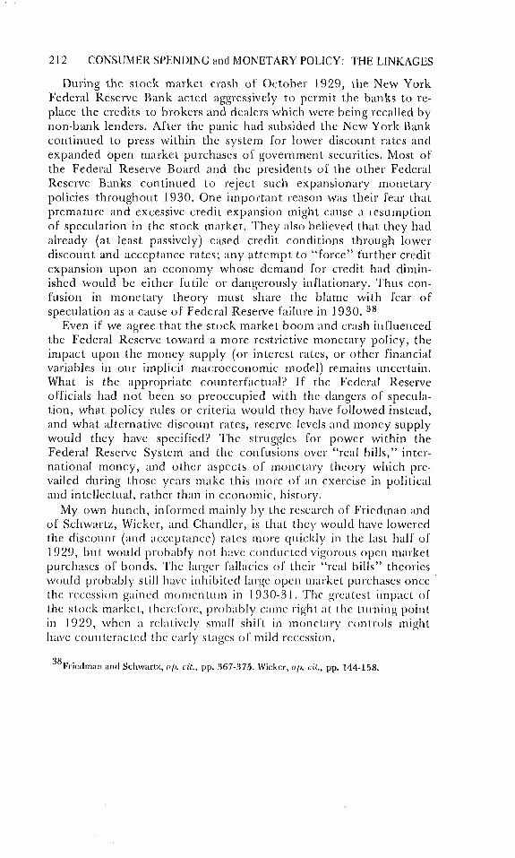
During the stock market crash of October 1929, the New YorkFederal Reserve Bank acted aggressively to permit the banks to re-place the credits to brokers and dealers which were being recalled bynon-bank lenders. After the panic had subsided the New York Bankcontinued to press within the system for lower discount rates andexpanded open market purchases of government securities. Most ofthe Federal Reserve Board and the presidents of the other FederalReserve Banks continued to reject such expansionary monetarypolicies throughout 1930. One important reason was their fear thatpremature and excessive credit expansion might cause a resumptionof speculation in the stock market. They also believed that they hadalready (at least passively) eased credit conditions through lowerdiscount and acceptance rates; any attempt to "force" further creditexpansion upon an economy whose demand for credit had dimin-ished would be either futile or dangerously inflationary. Thus con-fusion in monetary theory must share the blame with fear ofspeculation as a cause of Federal Reserve failure in 1930. a8
Even if we agree that the stock market boom and crash influencedthe Federal Reserve toward a more restrictive monetary policy, theimpact upon the money supply (or interest rates, or other financialvariables in our implicit macroeconomic model) remains uncertain.What is the appropriate counterfactual? If the Federal Reserveofficials had not been so preoccupied with the dangers of specula-tion, what policy roles or criteria would they have followed instead,and what alternative discount rates, reserve levels and money supplywould they have specified? The struggles for power within theFederal Reserve System and the confusions over "real bills," inter-national money, and other aspects of monetary theory which pre-vailed during those years make this more of an exercise in politicaland intellectual, rather than in economic, history.
My own bunch, informed mainly by the research of Friedman andof Schwartz, Wicker, and Chandler, is that they would have loweredthe discount (and acceptance) rates more quickly in the last half of1929, but would probably not have conducted vigorous open marketpurchases of bonds. Thc larger fallacies of their "real bills" theorieswould probably still have inhibited large open market purchases oncethe recession gained momcntum in 1930-31. The greatest impact ofthe stock market, therefore, probably came right at the turning pointin 1929, when a relatively small shift in monetary controls mightbavc countcraclcd the early stages of mild recession.
38Friedman and Schwartz, op. tit:., pp. 367-375. Wicker, op. cir., pp. 144-158.
CHANGE OF STOCK PRICES GREEN
VII. Other Channels of CausationBetween the Stock Market and the Economy
213
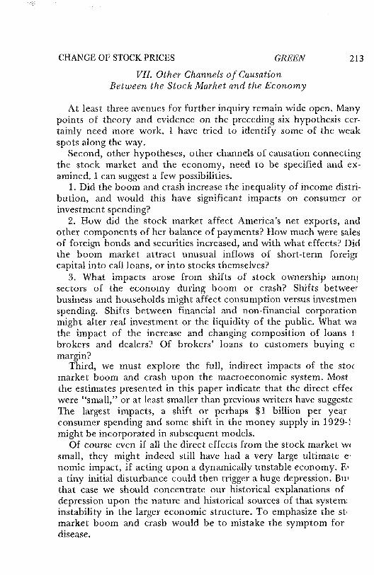
At least three avenues for further inquiry remain wide open. Manypoints of theory and evidence on the preceding six hypothesis cer-tainly need more work. I have tried to identify some of the weakspots along the way.
Second, other hypotheses, other channels of causation connectingthe stock market and the economy, need to be specified and ex-amined. I can suggest a few possibilities.
1. Did the boom and crash increase the inequality of income distri-bution, and would this have significant impacts on consumer orinvestment spending?
2. How did the stock market affect America’s net exports, andother components of her balance of payments? How much were salesof foreign bonds and securities increased, and with what effects? Didthe boom market attract unusual inflows of short-term foreigrcapital into call loans, or into stocks themselves?
3. What impacts arose from shifts of stock ownership amon!sectors of the economy during boom or crash? Shifts betweerbusiness and households might affect consumption versus investmenspending. Shifts between financial and non-financial corporationmight alter real investment or the liquidity of the public. What wathe impact of the increase and changing composition of loans tbrokers and dealers? Of brokers’ loans to customers buying cmargin?
Third, we must explore the full, indirect impacts of the sto(market boom and crash upon the macroeconomic system. Mostthe estimates presented in this paper indicate that the direct effe~were "small," or at least smaller than previous writers have suggesteThe largest impacts, a shift or perhaps $1 billion per yearconsumer spending and some shift in the money supply in 1929-!might be incorporated in subsequent models.
Of course even if all the direct effects from the stock market w~small, they might indeed still have had a very large ultimate e.nomic impact, if acting upon a dynamically unstable economy. E,a tiny initial disturbance could then trigger a huge depression. Bulthat case we should concentrate our historical explanations ofdepression upon the nature and historical sources of that system:instability in the larger economic structure. To emphasize the st.market boom and crash would be to mistake the symptom fordisease.
TABLE 1
DIVIDEND iNCOME
YEARS
1927192819291930193119321933
Dividends($ billions)
5.05.35.95.64,32,72.2
Change in Dividendsover previous year
{$ billions)
+0.3+0.3+0.6-0.3-1.3-1.6-0.5
Change inDividends as %of change in
National income
8%1929
11
Change inDividends as %of change in
Cnnsumer Spending
18%21
121423
~n opposite direction.
Source: Wlarvin Ho~enberg, "Estimates of Nationa| Output, Distributed income, Consumer Spending, Saving, and CapitaB Formation,’"Review of Economic Statistics, XXV (190,3}, 156,169.
ESTIMATION OF ANNUAL CAPITAL GAINS AND LOSSESON COMMON AND PREFERRED STOCKS
HELD BY NON-FARM HOUSEHOLDS(1922- 1933)
Change in Allocation of CapitalEnd of Year Stock Prices Stock Prices Gains or Losses
1922192319241925192619271928
Sept. 19291929
19301931
June 193219321933
75.173.988.1
106.7111,4141.2188,3237.8163.7
117,061,235.951.077.1
-1.214.218.6
4.729,847.149.5
-74.188,6-46.7-55,8-25.315.126.186,6
-$ 0.9 billion4
10.914,33.6
22.936.238.1-57.066,1
-$44.6 billion5
-53.2-24.1
14,424.9-82.6
Total capital gains from end of 1922 to end of 1929 ($68.097 billion) derived bytaking the change in holdings between those dates ($138.296 o 55.520 = $82.776billion)1 and subtracting the cumulation of saving in the form of corporate stocksduring the intervening years ($14.679 billion).2 Similarly, the total capital lossesbetween the end of 1929 and the end of 1933 ($82.646 billion) are derived bytaking the change in holdings ~$57.113 - 138,296 = $81.183 billion)1 and sub-tracting the cumulation of saving ($1.463 billion).2
These total capital gains and losses are then allocated on an annual basis accord-ing to changes in Standard and Poet’s Index of Common Stock Prices.3 In addi-tion, the peak ~September, 1929) and through (June, 1932) prices are used inorder to give an estimate of capital gains and losses to those dates.
1Raymond W. Goldsmith, Lipsey, and Mendelson, Studies in the National Balance
Sheet of the United States (New York, 1963), II, 319.
2Raymond W. Goldsmith, A Study of Saving in the United States (Princeton, 1955),I, 482 - 483.
3Board of Governors of the Federal Reserve System, Banking and Monetary Statistics(Washington, D.C., 1943), 480 - 481. The average of December and January priceswas used, in order to maintain comparability With Goldsmith’s data. See Studies in theNational Balance Sheet, I I, 15.
451.2 x68.097~ = $0.9
82.6465546.7 x8--8--~-.-.~-.6 = $44.6
TABLE 5
OWNERSHIP OF PREFERRED AND COMMON STOCK BY HOUSEHOLDS,AND CHANGES DUE TO SAVINGS AND CAPITAL GAINS (LOSSES)
($ BILLIONS)
YEARS Jan. 1 Holdings Saving1 Capital Gains2 Dec. 31 Holdings
1923192419251926192719281929
193019311932
1933
55.555;767.783.989,1
113.8152.9195.3 (Sept,)138.394,641,717.6(July)
32.0
1.11,11.91,61.82.94,3
0.90.30.0
0.2
-0.910,914.33,6
22,936.238.1
-57.0-44,6-53.2-24.114,424,9
55.767.783.989.1
113,8152.9195.3 (Sept.)
138,394,641.717.6 (July)
32;057.1
1 Raymond W. Goldsmith, A Study of Saving in the United States (Princeton, 1955),I, 482 - 483.
2Nly estimates, based on Goldsmith data, See previous table.
TABLE 6
VALUE OF STOCKS FROM ESTATE TAX RETURNSAND ESTIMATED CAPITAL GAINS IN YEAR OF DEATH
Source: Lawrence H. Seltzer, The Nature and Tax Treatment of Cap#al Gainsand Losses |NBER, New York, 1951), p. 367,
TABLE 8
STOCK YIELDS, EARNINGS/PRICE RATIOSAND NEW iSSUES OF STOCKS AND BONDS
YEARS
19231924t~251926192719283929
Sept. 192919301931
Yield onCommon Stock
{Percentages)
5.945~875.195.324.773.983.48
2.924.265.586.69
Earnings/PriceRatio
{Percentages)Financial Chronicle
{$ billions)
2.6353.0293.6053.7544.6575.3468.002
4.483
.325
11.3810,27
10.057,577,306,23
New issues of Stocks and BondsMo ody " s Investors Service
{$ billions)
1.6241.9411.8241.801%7811.4951.787
1.939.796.203
Sources: U.S. Bureau of the Census, Historical Statistics of the United States, Colonial Times to !957, pp. 656, 658.
George Eddy, "SecuriW I~ues and Reag Inv~ment in 19~," R~iew of Economic Statistics, XIX (1937}, 91.
Le~er V. Chandler, Am~can Moneta~ Polio, 1928-! 9~1 {New York, 1971), p, 28.
TABLE 9
BANK DEBITS AND DEPOSIT TURNOVER (VELOCITY),FOR DEMAND DEPOSITS IN COMMERCIAL BANKS
(1921 - 1933)
YEARS ALL COMMERCIAL BANKS
Debits Velocity($ billions)
1921
1922
1923
1924
19251926
1927
1928
1929
1930
1931
19321933
569
620
658
687
32.634.234.134.4
N. Y. CITY WEEKLY REPORTINGMEMBER BANKS
Debits Velocity
($ billions)
203 54.9
235 61.8234 66.5
258 66.5
307 71.9
332 77,8
384 85.3
490 106,3
592 124,4376 77.0
258 54.7
165 37,6
158 34.8
788 36,3
838 37.7
915 41,0
1075 46.8
1237 53.6
892 40,4
658 33,2
456 27,3
424 26.8
Source: Board of Governors of the Federal Reserve System, Banh, i~" andMoneta~2 Statistics IWashington, D.C., 1943), p. 254.
DISCUSSION
PHILLIP D. CAGAN
Did the 1929 stock market crash deepen the subsequent businessdepression? In the public’s view it did, but economists have beenskeptical. Now that wealth variables have recently made their wayinto consumption functions, a reappraisal of the 1929 crash is inorder. George Green’s paper re-examines the question and stillconcludes that the crash had minor effects on economic activity. Hispaper is concerned with measuring the size of the capital gains andlosses and then assessing the effect. I generally agree with hisconclusion that it had minor effects. Let me comment first on themeasurement of capital gains and losses and then on the wealthvariable and its effects.
Measurement of Capital Gains and Losses
Green’s figure for capital losses needs to be scaled down. By nostretch of the imagination can one say that the entire decline in stockprices in 1929-1933 helped to produce the business contraction.Stock prices fell first because business earnings fell and secondbecause there was a revaluation of dividend-price ratios. Only thesecond of these begins to approximate an independent effect of thecrash. A change in the market value of a given stream of dividends ison a different footing than a decline in dividend payments.
To be sure, nothing that happens in the stock market iscompletely independent of what goes on in the economy. A changein dividend-price ratios may be justified by business prospects. But at
Mr. Cagan is Professor of Economics, Columbia University.
222
DISCUSSION CAGAN 223
least it is largely determined within the stock market, in the sensethat it reflects the anticipations and preferences of marketparticipants. Changing preferences first overvalued stocks before1929 and undervalued them .afterward. The large reduction infinancial wealth allegedly constrained expenditures for bothconsumption and investment. But the part due to the decline individends reflected the reduction in activity and played noindependent role. After all, land values collapsed in the 1929-33debacle too, but I haven’t heard the depression blamed on that.
It seems to me to come closer to the usual view of the crash tocount just the amount due to the revaluation of dividend streams. Iwould make one further minor adjustment to exclude revaluationsreflecting changes in the level of interest rates. While this can beignored in the pre-crash period when corporate bond yields wereroughly constant, a small adjustment is needed for the subsequentperiod, when yields rose.
To calculate the capital gains up to the 1929 crash, I start with1925, well before most of the outlandish speculation began. Anotherstarting point would not give greatly different results. In Green’sTable 8 we find that the dividend yield on stocks fell 1.7 percentagepoints from 1925 to 1929. This is a change in preferences by marketparticipants--speculative fever if you like. We may recalculate themarket value of the 1929 dividend stream, using the 1925 dividendyield of 5.19 percent. The 1929 stream of $5.9 billion thus had acapitalized value of $114 billion. By the lower dividend yield in 1929of 3.48 percent, the capitalized value was $169 billion. The increaseof $56 billion is my estimate of the capital gain. It is anoverestimation, since it includes new issues. We should count just theincrease in value of new stock after it had been issued, but suchrefinements would not alter the general order of magnitude. Green’sfigure for the capital gain--which includes the rise in stock prices dueto both the increase in dividends and in dividend yields, but does notadjust for new stock issues--is given in his Table 5 as $115 billion forthe same period. By excluding the effects of dividend payments, wecut .his total in half.
On the down side we obtain a similar cut. From 1929 to 1932 thedividend yield rose 3.2 percent, of which 0.1 percent can beattributed to a rise in corporate bond yields. The 1929 dividendstream, when capitalized at the higher dividend yield prevailing in1932 and with an adjustment for the rise in bond yields, had amarket value of $90 billion, a decline from 1929 of $80 billion.
224 CONSUMER SPENDING and MONETARY POLICY: THE LINKAGES
Green’s figure for the capital loss is $179 billion, again over twice asmuch.
Effect of the Decline in Wealth
Now what was the effect of the decline in financial wealth on theeconomy? Conceivably it could have affected the demand for moneybalances, business investment, and consumer expenditures. In theusual demand function for money balances, real wealth has anelasticity of about unity. The crash reduced the demand for moneybalances, therefore, by the same percentage as the decline in totalwealth and thus, for a given money stock, stimulated the economy.While this effect is not usually attributed to the crash, suchstimulative effects, as well as the other depressing effects, should becounted. Given some of the crazy results we can sometimes derivefrom models, it might turn out that stock market crashes are goodfor the economy!
The effects usually mentioned, however, are those which affectexpenditures directly. A stock market decline can instill pessimismabout the business outlook and thus discourage investmentundertakings. It can also make everyone feel poorer and want toconsume less. It is this latter result which the so-called wealth effectis concerned with. Green uses a coefficient of .06 for the wealtheffect on consumption, which comes from some earlier work ofAndo and Modigliani. With the .06 coefficient, Green uses his figurefor a capital gain of $115 billion in the 1925-29 period to find thatconsumption was higher by $7 billion in 1929 compared with 1925.The capital losses thereafter imply that consumption in 1932 waslower compared with 1929 by $11 billion, which was 38 percent ofthe actual decline in comsumption.
This makes the wealth effect on consumption appear to be veryimportant. To obtain the independent effect, however, this figureshould be reduced to the lower capital loss figure (which Icalculated) of $80 billion. If we take .06 of that, we get $4.8 billion,which was 17 percent of the actual decline in consumption. Therevision is appropriate, because the coefficient was estimated from amultiple regression which held other influences on consumptionconstant. Only the part of the change in wealth uncorrelated withother influences should be counted. Moreover, this uncorrelated partwas probably a smaller fraction of the total decline in wealth in
DISCUSSION CA GAN 225
1929-32 than in the post-World War II period, when dividend streamswere fairly stable and most of the variation in stock prices reflectedrevaluation. The 17 percent figure still makes the crash appear to beimportant though not so eye.catching. To find the total effect on theeconomy, we should multiply by the total effect on aggregatlveexpenditures of an autonomous change in wealth. Based on fiscalmultipliers of current econometric models, the multiplier appears tolie between one and two.
Green argues that his estimate is probably too high. He points outthat a consumption function containing only permanent income doesnot have large residuals in the 1925-1932 period. You can see this inthe chart of the permanent income function that I fitted for MiltonFriedman in his study of the consumption function. It shows noimportant residuals during this period. In other words, we don’t needthe addition of market wealth to explain consumption in the1925-32 period. The decline in permanent income incorporates thedecline in dividends, and nothing seems to be left over for the rise individend-price ratios to explain. One might argue that there was a lagin the effect of the stock market decline and only when the capitallosses appeared to be permanent did people begin, to take them intoaccount in their consumption. But that would push the effects onconsumption into the middle or later 1930’s, at which timeconsumption was higher than the regression predicted, not lower assuch a lagged wealth effect would imply.
Green relies heavily on this evidence that the consumptionfunction without wealth fits the data fairly well. But, of course,one’s conclusion here depends on what importance he attaches to thewealth effect. According to the earlier Ando-Modigliani study,wealth has a significant independent effect. The issue is whetherchanges in the market value of wealth affect aggregate expendituresimportantly in the short run.
Increase in the Role of Monetary Effects
The recent attention to the wealth variable increases the role ofmonetary effects in the FRB-MIT econometric model, which islaudable. The early versions slighted those effects. Interest rates,although included in all the relevant equations, did not play a majorrole, whereas the market value of wealth enhances interest-rateeffects due to changes in monetary growth. This econometricapplication follows upon the lavish attention which the theoreticalliterature has paid to the wealth effects of money. The result in the
226 CONSUMER SPENDING and MONETARY POLICY: THE LINKAGES
FRB-MIT model is that wealth, and in particular the stock market,becomes the major channel of monetary effects on the economy.
I find this hard to believe. First of all, do people adjust theirconsumption to ephemerM changes in wealth? It is true that they donot know which way the market is going to change, so that currentstock prices are the best estimate of future discounted levels. Butthat doesn’t mean that consumption is adjusted as quickly to changesin stock prices as to an increase in wage and salary income. It is alsotrue that every time the stock market takes a plunge the Wall StreetJournal runs a story on how bad business is at Tiffany’s. No doubtthe stock market hits luxury expenditures, but such effects are verylimited. Moreover, it seems to me that Tiffany’s suffers more fromthe short-run psychological elation or despair of winning or losing inthe stock market than from an adjustment of consumption levels topermanent changes in wealth.
Moreover, conventional theory teaches (correctly I believe) thatchanges in monetary growth produce portfolio adjustments andsubstitutions among assets and affect expenditures through thesupply of loanable funds and the rates of return on assets. Thesesubstitution and liquidity effects are not fully represented by theusual expenditure equations because of the variety of channels andinterest rates involved, which are hard to measure with the availablestatistical techniques.
I am not denying that new money adds to wealth, but the increasein wealth due to a change in the money stock is usually insignificant.As the new emphasis on wealth implies, the important effect ofmonetary policy on wealth comes through changes in interest rates,which can produce large changes in the market value of wealth, andthis could no doubt have some effect on spending. But these arelikely to be transitory changes in wealth, while the main effects ofwealth on consumption will be those of a permanent nature. Thechanges in interest rates produced by variations in monetary growthtend to be temporary, aside from the effect of changes in theanticipated rate of increase of prices.
It would be helpful to re-examine the 1920’s and 1930’s with thenew consumption durables and other refinements. Either wealth hasentered.the equation spuriously, or it had a much greater effect in1929-33 than Green, I, and others believe. Perhaps the stock marketreflects changes in monetary growth without being a transmissionmechanism of monetary effects. Would it remain significant if oneput lagged monetary growth in as a proxy for channels of monetaryeffects otherwise omitted? Or possibly the wealth variable represents
DISCUSSION CAGAN 227
something else. Some recent work suggests that it is a proxy in theequations for consumer sentiment or expectations about the future.Sentiment and wealth are not conceptually the same thing, thoughthey might vary similarly over business cycles. Consumer sentimentdoes not work through the stock market, for the would limit itsinfluence to a relatively small group; and, while the stock marketmay influence consumer sentiment, so do many other things.
Whether on the right track or not, the present emphasis on wealthas a major channel of monetary effects gives an ironical twist to theold view that changes in wealth are an undesirable side effect ofmonetary policy. In the early 1950’s, for example, monetary policywas thought to require large changes in interest rates to be effective,and this was consi~lered dangerous precisely because it wouldproduce large variations in wealth. Recall Lawrence Seltzer’s 1946article entitled "Is a Rise in the Rate of Interest Necessary orDesirable?" in the American Economic Review. He. expressed awidespread view that variations in wealth could endanger thesolvency of financial institutions and, for that reason as well asothers, induce changes in consumer and business expectations andexpenditures which would be volatile and difficult to control. Seltzerwas concerned over possible increases in interest rates in the earlypost-World War II years, but similar views lay behind the.condemnation of stock market speculation in the 1920’s. The viewthat changes in wealth are a very clumsy and undesirable way tostabilize economic activity is still very strong. With the new emphasisof the Federal Reserve on growth of the monetary aggregates,monetary policy has to be willing to allow wide fluctuations ininterest rates and runs up against its long-standing tradition ofpreventing such fluctuations.
Extent of Recent Declines in Wealth
Recent experience has shown, however, that quite large declines irthe market value of securities can occur without seriomrepercussions on the economy. I have made some rough estimates olthe recent capital losses of the household sector from the flow olfunds account. In 1965 that sector held bonds worth $65 billionApplying the change .in an index of market yields for each borngroup, and assuming (to be on the low side) an average maturity othe bonds outstanding of only five years, the capital loss in markevalue up to 1970 was 13 percent. In addition, the cost of living ros,another 26 percent, so in real terms the decline was 36 percent. Jus
228 CONSUMER SPENDING and MONETARY POLICY: THE LINKAGES
from 1968 to 1970 the capital loss was 7 percent in nominal valueand 19 percent in real terms. Again for the household sector,corporate share holdings declined 14 percent from 1968 to 1970;adding in the price rise, there was a 25 percent decline in theircorporate share holdings in real terms.
Of course, actual wealth did not decline equally because of newsavings. If we look at the net financial worth of households, itnevertheless declined $49 billion, or 3 1/2 percent, from 1968 to1970. A decline in this total is an unusual occurrence, and even thesefigures do not allow for the market decline in bond prices, which theflow of funds takes at their maturity value. By my figures this wouldincrease the decline by another $6 billion. The total decline in wealthfrom 1968 to 1970 was about 16 percent in real terms. If we apply a.05 coefficient to the dollar change, consumption from 1968 to 1970would supposedly have been reduced $12 billion in real terms. Thatis a large figure. It excludes financial i.nstitutions, which also sufferedtremendous capital losses in terms of the market value of their assets.(Depreciation due to inflation is counted in the figures for depositholdings of the household sector.)
Yet what terrible consequences resulted from this gigantic declinein financial wealth? We did have the 1969-70 credit crunch, but itwas due to monetary restraint and not to the decline in wealth. Ifanything, the decline in wealth alleviated the crunch by inducingmore saving, which augmented the supply of loanable funds.Financial institutions were under strain, but much of that reflectedthe re-channeling of credit flows produced by deposit-rate ceilingsand other regulations and cannot be attributed to the decline in assetvalues. To be sure, savings and loan associations were technicallyinsolvent in 1969 with the sharp rise in mortgage yields; thatreflected a very special situation which everyone agrees needs to becorrected by institutional reforms.
Apart from financial institutions, what was the effect of thedecline in household wealth? Not all the evidence is in, but I do notdetect serious consequences for the economy. I believe we havevastly overrated the dangers of interest-rate fluctuations and theaccompanying changes in wealth. While they have some troublesomeside effects, they are not a high price to pay, when necessary, for aflexible monetary policy to stabilize national income and prices.Moreover, while interest rates may fluctuate more at times if policypays less attention to them, more stable monetary growth should, onthe whole, result in less fluctuation in interest rates as well as ineconomic activity.