The Economic Outlook for Fifth District States in 1984 ... · STATES IN 1984: FORECASTS FROM VECTOR...

THE ECONOMIC OUTLOOK FOR FIFTH DISTRICT

STATES IN 1984: FORECASTS FROM

VECTOR AUTOREGRESSION MODELS

Anatoli Kuprianov and William Lupoletti

I.

INTRODUCTION

According to the National Bureau of Economic

Research, the 1981-1982 economic recession ended in

November of 1982. Since then, the United States

economy has experienced a rapid recovery, evidenced

by reports of strong economic growth and a dramatic

decline in the unemployment rate. The strength of

the current economic expansion initially surprised

most analysts, although there now seems to be a

rapidly developing consensus that this expansion will continue through 1984. However, the renewed eco-

nomic growth apparent in the national economy has

not affected all regions of the country equally. This

article examines the implications of recent improve- ments in national economic conditions for the states

in the Fifth Federal Reserve District.1 The results of this analysis suggest that the economic growth

experienced by most Fifth District states in 1983 will

be sustained through the year ahead.

An outline of this article is as follows. First, the

cyclical variation in economic activity experienced by

Fifth District states over the past five business cycles

is compared with that experienced by the national

economy over the same period. This is followed by an examination of forecasts of real personal income

and total employment through the end of 1984 for each of the Fifth District states and for the U.S.

economy. These forecasts are produced using a purely statistical technique known as vector autoregression. The concluding section of the paper summarizes the results.

1 The Fifth Federal Reserve District includes the District of Columbia, Maryland, North Carolina, South Carolina, Virginia, and most of West Virginia.

II.

THE RECENT PERFORMANCE OF

FIFTH DISTRICT ECONOMIES

Data

In order to examine the past behavior of the econo-

mies of the states in the Fifth Federal Reserve Dis-

trict and to forecast future trends, this study focuses

on two measures of economic activity: real personal

income and total employment.

On the national level, the indicator that is most

often used to measure the overall performance of the economy is the gross national product. Gross state product is not commonly measured; the closest avail-

able substitute for GNP on the state level is personal

income. In order to separate the effects of inflation

from those of true economic growth, personal income

is divided by a measure of the national price level,

the implicit price deflator on personal consumption

expenditures, to yield real (inflation-adjusted) per-

sonal income.

Another closely watched economic indicator is the

unemployment rate. However, consistent quarterly

data on unemployment rates for all states in the Dis-

trict are only available starting in 1965. Measures of

total employment, on the other hand, begin in 1958.

This study concentrates on total employment in order

to capitalize on the availability of a larger data set.2

2 Employment data for this study comes from the Bureau of Labor Statistics’ survey of business establishments, which does not include farms. Farm employment is not ordinarily very sensitive to changes in business cycle conditions. Therefore, movements in total nonagricultural employment should be similar to those in total employment including farms, and using nonfarm employment as a proxy measure of total employment should not cause much distortion.

12 ECONOMIC REVIEW, JANUARY/FEBRUARY 1984

In an analysis of regional economies, it is important

to know whether the data series being employed are

measured by place of work or by place of residence.

This distinction is especially crucial for the District

of Columbia, where a large portion of the labor force

lives outside the city limits. The relevant questions

to ask about the performance of the District of

Columbia economy are: (1) Is the income of its

residents increasing or decreasing, and (2) Is em-

ployment within its boundaries increasing or decreas-

ing? Statewide total employment measured by place

of work is the only data series available, but personal

income is measured both ways. This study employs

personal income measured by place of residence.

Data on both personal income and total employment

for the states are available in seasonally adjusted

form beginning in 1958 on the Chase Econometrics

Regional Macro data base. The National Bureau of

Economic Research has determined that five complete

business cycles, measured trough-to-trough, occurred

between the second quarter of 1958 and the fourth

quarter of 1982.3 Although peak-to-peak measures

3 Business cycle troughs, marking the end of a recession and the beginning of an expansion, occurred in the second quarter of 1958, the first quarter of 1961, the fourth quarter of 1970, the first quarter of 1975, the third quarter of 1980, and the fourth quarter of 1982. Dates of cyclical peaks are 1960Q2, 1969Q4, 1973Q4, 1980Q1, and 1981Q3.

are more common in the analysis of business cycles,

adopting a trough-to-trough convention allows a more

complete use of the available data in this instance

(since only four complete peak-to-peak cycles have

occurred since 1958) and leads to the same general

conclusions about the performance of the state econo-

mies.

Table I summarizes the recent history of economic

growth, as measured by personal income and total

employment, of Fifth District states over the last

quarter century. The table shows that the economic,

growth experienced by the states of the Fifth District

was greater than that of the national economy over

this period. Four of the six states in the District had

higher rates of growth of income and employment

than did the nation. North Carolina, South Carolina,

and Virginia grew at least as much as the U. S. over

each of the five business cycles. Virginia was the

most consistent of all: it outperformed the national

economy in every ‘business cycle of the last 25 years.

On the other hand, the District of Columbia grew

more slowly than the nation in every cycle except the

first. The Fifth District’s rate of economic growth

slowed somewhat during the past decade, though. Since 1975, the District as a whole appears to have

lagged slightly behind the nation’s rate of expansion.

Table I

PERFORMANCE OF FIFTH DISTRICT ECONOMIES OVER THE LAST FIVE BUSINESS CYCLES

Note: Data are annualized compound growth rates, expressed as percentages.

FEDERAL RESERVE BANK OF RICHMOND 13

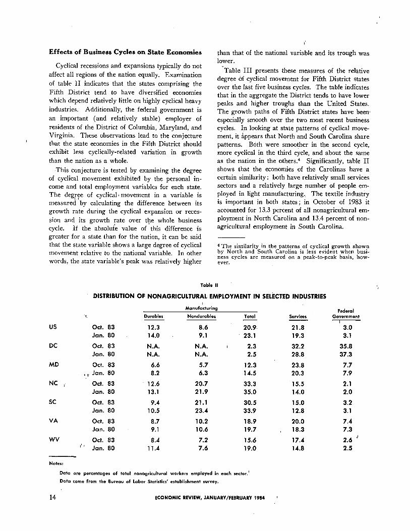
Effects of Business Cycles on State Economies

Cyclical recessions and expansions typically do not

affect all regions of the nation equally. Examination

of table II indicates that the states comprising the

Fifth District tend to have diversified economies

which depend relatively little on highly cyclical heavy

industries. Additionally, the federal government is

an important (and relatively stable) employer of

residents of the District of Columbia, Maryland, and Virginia. These observations lead to the conjecture

that the state economies in the Fifth District should

exhibit less cyclically-related variation in growth

than the nation as a whole.

This conjecture is tested by examining the degree

of cyclical movement exhibited by the personal in-

come and total employment variables for each state.

The degree of cyclical movement in a variable is

measured by calculating the difference between its

growth rate during the cyclical expansion or reces-

sion and its growth rate over the whole business

cycle. If the absolute value of this difference is

greater for a state than for the nation, it can be said

that the state variable shows a large degree of cyclical

movement relative to the national variable. In other

words, the state variable’s peak was relatively higher

than that of the national variable and its trough was

lower.

Table III presents these measures of the relative

degree of cyclical movement for Fifth District states

over the last five business cycles. The table indicates

that in the aggregate the District tends to have lower

peaks and higher troughs than the United States.

The growth paths of Fifth District states have been

especially smooth over the two most recent business

cycles. In looking at state patterns of cyclical move-

ment, it Appears that North and South Carolina share

patterns. Both were smoother in the second cycle, more cyclical in the third cycle, and about the same

as the nation in the others.4 Significantly, table II

shows that the economies of the Carolinas have a certain similarity: both have relatively small services

sectors and a relatively large number of people em-

ployed in light manufacturing., The textile industry

is important in both states; in October of 1983 it

accounted for 13.3 percent of all nonagricultural em-

ployment in North Carolina and 13.4 percent of non-

agricultural employment in South Carolina.

4 The similarity in the patterns of cyclical growth shown by North and South Carolina is less evident when business cycles are measured on a peak-to-peak basis, however.

Table II

DISTRIBUTION OF NONAGRICULTURAL EMPLOYMENT IN SELECTED INDUSTRIES


Table III

RELATIVE DEGREE OF CYCLICAL MOVEMENT

IN FIFTH DISTRICT STATES

Degree of cyclical movement is measured as the rate of

growth of the variable during the business cycle expansion

minus its rate of growth during the whole business cycle,

and as the rate of growth aver the whole cycle minus the

rate of growth during the cyclical recession.

Relative degree of cyclical movement is the comparison be-

tween the degree of cyclic+ movement of the state variable

and that of the U. S. variable.

M means the state showed mare cyclical movement than did

the U.S.; in other words, the state variable had a higher

peak and a lower trough than did the U. S. variable.

L means the state showed less cyclical movement than did

the U.S.; in other words, the state variable moved along a

smoother path than did the U. S. variable.

A means the state and national experiences were similar.

Z means the data are ambiguous and cannot be clearly

interpreted.

Real personal income and total employment are the variables

used.

The District of Columbia’s pattern is remarkably

consistent : in every business cycle its economy has

moved on a significantly smoother path than has the economy of the United States. To put it another

way, the District of Columbia has grown at a rate very close to its trend during all phases of the last

five business ‘cycles. This is hardly surprising, since

the federal government employs more than one out of

every three workers in the nation’s capital, making it

the city’s largest employer. Over the postwar period,

the federal government has grown at a steady rate

regardless of the phase of the business cycle. Evi-

dently the steady growth of government has swamped any cyclical behavior in the District of Columbia,

making the growth path of its economy a remarkably

smooth one. The paths of Maryland and Virginia,

the two other Fifth District states in which the federal

government is a major employer, have also been less

cyclical than the nation as a whole. Both Maryland

and Virginia are also characterized by relatively large

service industries and relatively small amounts of

heavy industry.

West Virginia’s economy has exhibited patterns of

growth which are quite different from those of the

other states in the District. The economy of West

Virginia is strongly influenced by the coal-mining

industry: at the business cycle peak in January of

1980, 10.4 percent of all workers in West Virginia

were employed in the mining industry. As a result,

factors affecting this industry can overwhelm the

effects of changes in national economic conditions.

For example, United Mine Workers’ strikes are ap-

parently responsible for the severe oscillations evident

in the West Virginia personal income and total em-

ployment series pictured in chart 1.6

The 1973-1975 recession also illustrates the im-

portance of the coal industry to West Virginia’s

economy. The onset of the recession coincided with

the so-called “energy crisis,” when the price of oil in

the United States increased dramatically. Increases

in the price of oil drove up the demand for coal; as a

result, while the U. S. economy experienced a severe.

recession, West Virginia prospered. During the

1973-1975 national recession, West Virginia personal

income grew at a 4.4 percent annual rate, similar to the growth rates in each of the two expansions sur-

rounding the recession (4.8 and 4.2 percent, respec-

tively).

More recently, economic conditions in West Vir-

ginia appear to have deteriorated greatly. Economic

growth was brought to a halt in the 1980 recession,

and the state’s economy seems not to have fully re-

covered since that time. The mining industry has

been especially hard hit in the eighties : the number of people employed in West Virginia’s mining indus-

try fell 23 percent from January 1980 to October

1983, from 66,400 to 50,900. It would appear once again that conditions in the coal industry are a crucial

factor affecting economic growth in West Virginia.

Timing of Peaks and Troughs

The preceding analysis has assumed that turning

points of the state personal income and employment

series coincide with national business cycle turning

5 When the UMW struck in the second quarter of 1981, West Virginia’s personal income fell 21.8 percent and total employment dropped 23.7 percent; when the union returned to work in the following quarter, income rose 36.4 percent and employment gained 30.3 percent. Similar movements in the income and employment series occurred at the times of the UMW strikes of 1978Q1 and 1971Q4.


points. This assumption is consistent with the U. S.

Commerce Department’s classification of national

personal income and nonagricultural employment as

coincident indicators of the business cycle. Never-

theless, it is possible that movements in measures of a

particular state’s economic activity could precede or

lag movements in the corresponding national variable.

The timing relationships between state and national

variables were examined using a statistical technique

known as a Granger-causality test.6 In a Granger-

causality test, one observes whether the past history

of a variable X can help to predict the current out-

come of another variable Y, given the past history of

Y. If past X helps to predict current Y, X is said

to Granger-cause Y. Care must be taken in inter-

preting the results of such tests; the term “causality test” used in this context is somewhat misleading,

although it is standard nomenclature. Finding that a

variable X Granger-causes Y is neither necessary nor

sufficient evidence to support the conclusion that

observed changes in Y are a direct result of changes

in past X. For example, it may be that both X and

Y have a common cause, but the effects of changes in

this underlying cause become apparent in movements

in the variable X before changes in Y are observed.

It is also possible that changes in the currently observed value of X help to predict the current reali-

zation of the variable Y, given Y’s past history. In this case, X is said to Granger-cause Y instantane-

ously. Once again, it may be the case that currently

observed changes in both X and Y, while being highly

correlated, are the result of a third variable driving

both of the others. In the context of the present

analysis, it is not unreasonable to suppose that ob-

served changes in state personal income and employ-

ment occurring over a business cycle are a result of many of the same factors which also affect the corre-

sponding national macroeconomic variables. Never-

theless, changes in overall economic conditions may become apparent in certain regions either before or

after changes in national economic conditions become

noticeable. In the present analysis, Granger-causality

tests were employed in an effort to uncover evidence on the timing of cyclical peaks and troughs for Fifth

District states.

None of the states in this group was found to sys- tematically lead or lag the nation in both measures of

economic activity considered here, namely personal

income and nonagricultural employment. The tests

suggest that changes in North Carolina and South

6 The statistical theory underlying this technique is described in Granger (1969, 1980).

Carolina personal income tend to lag changes in U. S.

personal income over the 25-year period. Maryland

nonagricultural employment appears to lag changes in

national nonagricultural employment, while changes

in Virginia employment appear to lead national changes. The remaining tests found evidence of

strong contemporaneous relationships between state

variables and their national counterparts. Overall,

the results are not inconsistent with the hypothesis

that the economies of the Fifth District states reach

cyclical peaks and troughs roughly coincidental with

those of the national business cycle.

Ill.

FORECASTS OF FIFTH DISTRICT

ECONOMIC CONDITIONS

Regional Forecasting Models

The forecasts presented in table IV were prepared

using vector autoregression (VAR) models. Appli-

cation of VAR models to economic forecasting prob-

lems is a relatively recent development.7 Unlike the

more familiar structural econometric models em-

ployed by commercial forecasters and government

agencies (which are purportedly based on economic theory), VAR models represent a purely statistical approach to forecasting applications.

Structural models attempt to reproduce the work-

ings of an economic system with a set of simultaneous

equations. Each of these equations attempts to incor-

porate some theoretically predicted aspect of economic behavior. In contrast, restrictions on the

relationships among different economic variables that

are suggested by various theories are typically ig-

nored in the VAR models. A forecast of a given

variable obtained using a VAR model is based solely

on the observed history of that variable and the

history of a number of other related variables.

As a practical matter, movements exhibited by

economic time series tend to be highly correlated.

Since VAR forecasts rely solely on the correlations

existing among. different variables, this approach

seems well-suited for economic forecasting applica-

tions. Moreover, because VAR models ignore the

complicated interrelationships among all the variables

of an economic system predicted by theory, they

require much less time, effort, and attendant cost to

7 Application of the VAR model for forecasting economic time series was largely popularized by Sims (1980). Anderson (1979) applied the VAR model to regional forecasting problems.


implement and are especially useful when the fore-

casting problem at hand is concerned with a very small number of variables. Structural models, if well-

specified, are more efficient for large-scale forecasting

applications. The cost of implementing such models, however, may be quite high.8

VAR models have one noteworthy limitation. Be-

cause they embody no economic theory, such models

are not appropriate for the analysis of the effects of

changes in economic policy. Lucas (1976) and Sar-

gent (1981) have argued forcefully that a careful

analysis of the effects of changes in economic policy

(e.g., a significant change in tax rates or a choice of a

new operating target for monetary policy) must take into account the effects of this policy change on the

behavior of individuals. They argue that changes in

economic policy may be expected to alter the observed

behavior of individuals in the market because differ-

ent policies change the economic environment, or set,

of incentives, faced by these decision makers. Failure

to account for such effects can result in erroneous

policy conclusions. McCallum (1982), among others,

has criticized the use of VAR models for policy

evaluation precisely on the grounds that such models

are subject to Lucas’ criticism. As a consequence,

the forecasting performance of VAR models may be expected to deteriorate in periods when significant

policy changes occur.

However, existing structural econometric models

have similar limitations. While such models attempt

to capture important aspects of economic behavior, it

has been argued they have not been entirely success-

ful in attaining this goal; Lucas’ policy evaluation

critique was initially directed at the methodology

underlying structural models existing at that time.

Despite the subsequent widespread acceptance of

Lucas’ arguments, the methodology employed by

most forecasters has not really changed. As Sims

(1980) has noted, much of the “theory” underlying existing large-scale econometric models is largely ad

hoc; that is, restrictions imposed on the models are likely to reflect analytically convenient assumptions

or empirical regularities apparent in existing data

samples rather than being a result of predictions

based on a coherent theory of economic behavior.

As a consequence, the forecasting performance of

such models is likely to be subject to’ many of the

same limitations stated’ above in connection with

VAR models. Forecasts obtained using VAR

models would therefore appear to offer a viable low-,

8 See Anderson (1979) for a comparison of the relative costs of these two forecasting methods.

cost alternative technique for regional forecasting problems.

A separate five-variable VAR model was con-

structed for each of the states in the Fifth District.

Each VAR model uses two statewide and three na-

tional variables.9 The state variables are total non-

agricultural employment and real personal income.

The three national variables common to all the models

are the six-month commercial paper rate, the index

of industrial production, and the M1 measure of the

money supply. All variables except the commercial

paper rate were expressed in the form of percentage

changes from the previous quarter. The models were

estimated using data for the time period 1958Q1

through 1983Q2, which was the longest sample

period available at the time of this writing. To facili-

tate the evaluation of the state forecasts, national real

personal income and nonagricultural employment

forecasts obtained from a national five-variable VAR

model were also included. Following the example of Anderson (1979), the

state variables were excluded from the equations used to forecast each of the three national variables. This

restriction reflects the prior belief that the state vari-

ables would not be useful in forecasting the national

variables, given that lags of each of the latter were

present in each of the forecasting equations. The VAR model used to forecast national personal income and employment incorporated no such restrictions,

however.

Survey of the Forecasts

Table IV and chart 1 summarize the forecasts

produced using the VAR models described above.

Since the regional data were available only through

the end of the second quarter of 1983 at the time the

forecasts were prepared, forecasts for the last two

quarters of 1983 were included. (Data on all

national variables were available through the third

quarter of 1983). These forecasts were obtained as a

by-product of producing the 1984 forecasts. The VAR forecast for U. S. real personal income

growth for all of 1983 is 4.2 percent. Total U. S.

nonagricultural employment was forecast to grow at a

2.8 percent annual rate for all of 1983. For 1984 the

forecasts suggest that a slightly different pattern of

growth will evolve-growth in real personal income

is forecast to fall somewhat from its 1983 rate, to 3.2

percent (still a healthy increase); growth in total

9 The West Virginia model included dummy variables to capture the effects of strikes by the United Mine Work- ers.


Chart 1

ACTUAL AND PREDICTED ECONOMIC GROWTH FOR FIFTH DISTRICT STATES

DISTRICT OF COLUMBIA

PERSONAL INCOME TOTAL EMPLOYMENT


Notes: Data are quarter-to-quarter annualized compound growth rates, expressed as percentages. Solid lines repre-

sent actual values from 1975 Q1 to 1983 Q2. Dotted lines represent forecast values from 1983 Q3 to 1984

Q4. Horizontal lines show the trend rate of growth from 1975 Q1 to 1983 Q2. Shadings mark peaks and

troughs of national business cycle. Tic marks correspond to first quarter of each year.


US

DC

MD

NC

SC

VA

WV

Table IV

FIFTH DISTRICT PERSONAL INCOME AND

TOTAL EMPLOYMENT FORECASTS

FROM VAR MODELS

1982 Total 1983 Total 1984 Total

(actual) (forecast) (forecast)

P.I. - 0.3 4.2 3.2

Emp. - 2.5 2.8 4.2

P.I. 1.6 2.3 0.9

Emp. - 1.5 0.6 1.0

P.I. 1.4 4.3 1.6

Emp. - 1.8 0.8 3.8

P.I. 0.4 8.0 6.2

Emp. - 2.2 3.5 7.2

P.I. - 0.1 7.4 5.3

Emp. - 2.9 5.0 7.6

P.I. 1.6 6.1 4.4

Emp. - 1.3 3.2 5.4

P.I. - 3.9 - 1.4 - 0.5

Emp. - 6.4 - 4.0 - 0.7

Notes:

Data are annualized compound growth rates, expressed as

percentages.

1983 total is based on forecasts for the last two quarters of

the year.

1983 total for US is based on a forecast for the last quarter

only.

nonagricultural employment, on the other hand, is

expected to rise to 4.2 percent. An increase in non-

agricultural employment of this magnitude would be

consistent with an unemployment rate of under 7

percent by the end of 1984.10 This is well below the

consensus of other publicized forecasts, and would

probably be regarded by most analysts as an overly

optimistic prediction. It is probably reasonable to

expect a slightly lower growth rate of employment to

be realized in the year ahead.

According to the VAR forecasts, four of the six states in the Fifth District will experience growth in

10 The total employment forecast can be combined with guesses about the growth of the labor force to produce estimates of the unemployment rate in 1984. If the labor force grows by 0.9 percent, as it did in 1983 (measured November over November), the resulting unemployment rate in November of 1984 would be 5.4 percent. labor force grows 2.5 percent, a rate that would make its 1983-1984 growth equal to the average growth rate experienced in the first two years of the last five recoveries, then the unemployment rate would be 6.8 percent. These two estimates can be considered the upper and lower bounds of unemployment rates consistent with 4.2 percent growth in total employment over 1984.

real personal income which is roughly equal to

(Maryland) or is greater than (North Carolina,

South Carolina, and Virginia) the rate of growth

forecast for the United States as a whole. The latter three states are also forecast to experience a higher

rate of growth in total employment than will the

national economy; however, Maryland total employ-

ment growth will be less than that of the United

States. Both the District of Columbia and West Vir-

ginia are forecast to continue to grow more slowly than the national economy in 1983.

For 1984 the forecasts indicate that each of the

states in the Fifth District, with the exception of

West Virginia, will experience a lower growth rate

of personal income and higher growth in total em-

ployment than in 1983. Notice that this is similar to

the pattern of growth predicted for the United States

as a whole over the 1983-1984 period. The VAR

forecasts suggest that three of the states in the Dis- trict (North Carolina, South Carolina, and Virginia)

will again experience faster growth than the national

economy in the coming year. The forecasts for the

District of Columbia and Maryland predict continu-

ing positive growth for 1984, but at a rate lower than

that expected for the U. S. economy. Finally, the

forecasts suggest the economy of West Virginia will continue to lag in the current economic recovery. The

growth rate of West Virginia real personal income

will average -0.5 percent in 1984; it also appears

that total employment will decline further in the

coming year (note, however, that the attached charts

show a predicted gradual improvement throughout

the year).

In summary, the VAR forecasts predict continuing

economic improvement for the United States and for

Fifth District states. The performance of the District

of Columbia, Maryland, and West Virginia econo-

mies will be modest but greatly improved over 1982. Unusually strong growth is predicted for North

Carolina, South Carolina, and Virginia through 1984.

However, the forecasts for employment growth, both for the nation as a whole and for the individual states,

may prove to be overly optimistic.

Evaluation of Model Performance

One criterion commonly used to evaluate the per-

formance of forecasting models is the analysis of out-

of-sample forecast errors. Out-of-sample forecasts for

the period 1980Q1 through 1983Q2 were produced

for all seven VAR models. The resulting values of

the average root mean square errors (RMSE) for

each VAR model are listed in table V. Forecast


errors for forecasting horizons of two through six

periods ahead were calculated as the difference be-

tween the average realized growth rate over the

forecast horizon and the average growth rate forecast

for the same period. The general pattern noticeable

in the results contained in table V is that the average

RMSE becomes smaller as the forecast horizon

ranges between one to four, five, or six quarters. It

would appear that the quarterly forecast errors

largely offset each other for forecast horizons in the

neighborhood of one year ahead. This pattern would

presumably not continue for arbitrarily large forecast

horizons-past some horizon (which appears to be

in the range of five to six quarters for these VAR

models), one would expect to observe successively

larger average forecast errors.

Average forecast errors for these models are rather

large for the 1980-1983 period. For example, the

average RMSE for the two-period ahead forecast for

District of Columbia personal income is about 5.6

percentage points. This compares with an average

growth rate of 2.0 percent for this variable over the

1958-1982 sample period. The first impression one

gets from looking at these results is that the forecasts

are not very precise. However, this particular time

period was a turbulent one for the U. S. economy.

For instance, the United States experienced two

separate recessions during this brief time. In addition

the period was characterized by important changes in

tax laws, the imposition of credit controls in 1980,

unusually large fluctuations in money growth, and

rapid regulatory decontrol of the banking system.

The earlier discussion of the limitations of VAR

models noted that these models may be expected to

produce poor forecasts in periods when major

changes in economic policy occur. Most of the major

policy changes that occurred during this time were

enacted in 1980 and 1981. Since that time money

growth has become slightly more predictable and no

other major policy initiatives have been introduced

(although two scheduled tax cuts have gone into

effect). Moreover, it appears that no significant new

policy initiatives will be forthcoming in 1984. Hence,

there is reason to believe that an analysis of average

forecast errors over the more recent 1982-1983 period

might be more relevant for drawing inferences about

the expected errors associated with the 1984 fore-

casts.

Table V

ERRORS FROM VAR FORECASTS MADE IN THE 1980s

Notes:

Sample includes forecasts mode with data ending in 1979:4 through forecasts mode with data

ending in 1983:2.

Errors are root mean square errors, expressed as percentage points.


Table VI shows that the VAR models produce much more accurate out-of-sample forecasts on aver-

age over the post-1981 period. This improvement is

especially noticeable for the shorter term forecasts

and for forecasts of the personal income variable at

all horizons. It should be kept in mind that the post-

1981 period, while less volatile than the previous two

years, was a period in which the U. S. economy

experienced a cyclical trough, and business cycle

turning points are typically difficult to forecast. The

performance of these forecasting models over this

period is encouraging. In view of the average errors

reported in table VI, the VAR forecasts should

prove to be reasonably accurate and therefore useful

in assessing regional business conditions for the year

ahead.

IV.

SUMMARY AND CONCLUSIONS

This paper has presented a brief statistical history

of the patterns of economic growth experienced by Fifth District states over the past 25 years, and vector

autoregression forecasts of real personal income and total nonagricultural employment for both the United

States economy and Fifth District states for 1984.

Comparing the forecasts with evidence available from

the last five business cycle expansions, it appears that

the U. S. economy will continue to experience a

normal recovery from recession in the year ahead.

Growth in U. S. real personal income is projected to average 3.7 percent per year over 1983 and 1984;

this is slightly below the average rate of growth for

this variable in the last five cyclical expansions.

Total U. S. nonagricultural employment is forecast

to grow at a 3.5 percent annual rate over the 1983- 1984 period; this is a full percentage point above the

average growth rate over the last five expansions for

this variable. An examination of unemployment rates

consistent with the VAR forecast for total employ-

ment growth in 1984 suggests that this forecast might

be expected to err on the high side.

The VAR forecasts point to a strong improvement in total employment throughout the Fifth District.

Five of the six states in the District are predicted to

experience employment growth over the 1983-1984

period at rates that are at least equal to their average

growth rates over the last five business cycle recov-

eries. The outlook is especially favorable for North

Carolina, South Carolina, and Virginia. These three

states are forecast to experience growth rates of both

personal income and total employment that are

Table VI

ERRORS FROM THE LAST SIX VAR FORECASTS

Notes:

Sample includes all forecasts made of 1982:1, 1982:2, 1982:3, 1982:4, 1983:1, and 1983:2.

Errors ore root mean square errors, expressed as percentage points.


greater than the growth rates expected for the nation

as a whole. The predicted rates of cyclical expansion

for these states are well above their historical aver-

ages. In fact, if the forecasts prove to be correct, the

expansion in North Carolina will be the strongest in

the last 25 years and both South Carolina and Vir-

ginia will turn in ‘their best economic performances

in over a decade. Both the District of Columbia and Maryland should

experience continued economic growth, although

neither is forecast to do as well as the nation as a

whole. The predicted growth rates of personal in-

come for these states are slightly lower than those

observed in past recoveries, while employment growth

is expected to be about average. The rate of growth

of total employment in Maryland should show sub-

stantial improvement during the year ahead: 1983

total employment growth will only be 0.8 percent,

but the VAR forecast calls for a healthy 3.8 percent

rate of growth in 1984. As has been the case in the

past, the economy of the District of Columbia should

continue to experience slow and steady growth in

the year ahead.

Real personal income in West Virginia is predicted to decline at an average annual rate of 0.5 percent in

1984, and total employment is expected to decline an average 0.7 percent over the year. If these forecasts

Sims, Christopher A. “Macroeconomics and Reality.” Econometrica 48 (January 1980), l-48.

are correct, they will represent a great improvement

for the West Virginia economy over the recent past;

additionally, the quarter-by-quarter forecasts pictured

in chart 1 point to a gradual improvement over the

course of the year.

References

Anderson, Paul A. “Help for the Regional Forecaster: Vector Autoregression.” Quarterly Review, Fed- eral Reserve Bank of Minneapolis 3 (Summer 1979), 2-7.

Granger, C.W.J. “Investigating Causal Relations by Econometric Models and Cross-Spectral Methods.” Econometrica 37 (July 1969), 424-438.

“Testing For Causality: A Personal View- point.“’ Journal of Economic Dynamics and Control 2 (1980), 329-352.

Lucas, Robert E. “Econometric Policy Evaluation : A Critique.” In Carnegie-Rochester Conference Series in Public Policy, vol. 5, ed. by K. Brunner and A. H. Meltzer. Amsterdam: North Holland, 1976.

McCallum, Bennett T. “Macroeconomics After a Decade of Rational Expectations: Some Critical Issues.” Economic Review, Federal Reserve Bank of Richmond 68 (November/December 1982), 3-12.

Sargent, Thomas J. “Interpreting Economic Time Series.” Journal of Political Economy 89 (April 1981), 213-248.

The Federal Reserve Bank of Richmond is pleased ‘to announce new editions of

two publications.

BUSINESS FORECASTS 1984

Edited by Sandra D. Baker

This publication is a compilation of representative business forecasts for the

coming year. It also contains a consensus forecast for 1984.

BUYING TREASURY SECURITIES AT FEDERAL RESERVE BANKS

8th Edition

These publications may be obtained free of charge by writing to:

Public Services Department Federal Reserve Bank of Richmond

P. O. Box 27622 Richmond, Virginia 23261


Date post:	27-Jul-2018
Category:	Documents
Upload:	trannhan
View:	212 times
Download:	0 times

The Economic Outlook for Fifth District States in 1984 ... · STATES IN 1984: FORECASTS FROM VECTOR...

Documents