THE ECONOMICS OF RELATIONSHIPS * Larry Samuelson Department of Economics University of Wisconsin 1180 Observatory Drive Madison, Wisconsin 53706 USA [email protected]October 9, 2005 * This paper was prepared for presentation at the 2005 World Congress of the Econometric Society in London. I thank Georg N¨ oldeke for comments. I am grateful to George Mailath for a long collaboration that culminated in Mailath and Samuelson (2006), from which this paper draws heavily. I thank the National Science Foundation (SES-0241506) for financial support.
∗This paper was prepared for presentation at the 2005 World Congress of the Econometric Society in
London. I thank Georg Noldeke for comments. I am grateful to George Mailath for a long collaboration
that culminated in Mailath and Samuelson (2006), from which this paper draws heavily. I thank the
National Science Foundation (SES-0241506) for financial support.
The Economics of RelationshipsLarry Samuelson
1 Introduction
1.1 Relationships: Two Illustrations
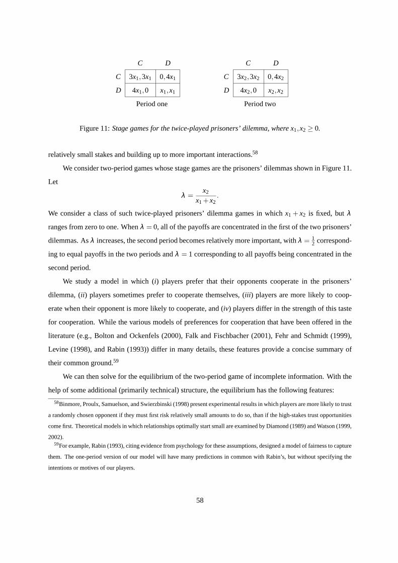
Each year, about$60billion dollars worth of diamond jewelry is sold worldwide. Over the course of its
journey from mine to warbrobe, a diamond typically passes through numerous intermediaries in search of
just the right buyer. Because diamonds are easy to conceal, difficult to distinguish, portable and valuable,
the opportunity to cheat on diamond deals are many. One would accordingly expect them to be handled
with the utmost care. To the contrary, virtually no care at all is taken:1
Once gems leave the vault-like workshops, they do so in folded sheets of tissue paper, in the
pockets of messengers, dealers and traders. They are not logged in and out ... or marked
to prevent substitution. They are protected from embezzling only by the character of those
who transport. ... On that slender record, gems worth thousands of dollars traverse the street
and are distributed among buyers from Bombay to Buenos Aries, Pawtucket and Dubuque.
In Puccini’s operaGianni Schicchi, the deceased Buoso Donati has left his estate to a monastery,
much to the consternation of his family.2 Before anyone outside the family learns of the death, Donati’s
relatives engage the services of the actor Gianni Schicchi, who is to impersonate Buoso Donati, write a
new will leaving the fortune to the family, and then feign death. Anxious that Schicchi do nothing to risk
exposing the plot, the family explains that there are severe penalties for tampering with a will and that
any misstep puts Schicchi at risk. All goes well until the time arrives for Schicchi to write the new will,
at which point he instructs that the entire estate be left to the great actor, Gianni Schicchi. The relatives
watch in horror, afraid to object lest their plot be exposed and they pay the penalties with which they had
threatened Schicchi.1This account of diamond transactions is taken from Richman (2005) (the sales figure from page 10 (footnote 29) and the
quotation from page 14 (noting that it is originally from an article by Roger Starr, “The Real Treasure of47th Street,” in the
New York Times(March 26, 1984, Section A, page 18))).2The use ofGianni Schicchito illustrate the (lack of) incentives in an isolated interaction is due to Hamermesh (2004, p.
164).
1
The outcomes in these situations are strikingly different. Those involved in the diamond trade face
constant opportunities to return one less diamond than they received, with the recipient unable to prove
they had been shortchanged, but refrain from doing so. Gianni Schicchi sees a chance to steal a fortune
and grabs the money. The diamond handlers are involved in a relationship. They know they will deal
with one another again, and that opportunistic behavior could have adverse future consequences, even
if currently unexposed. Gianni Schicchi was not involved in a relationship with the family of Buoso
Donati. Nothing came into play beyond the current interaction, which he turned to his advantage.
Throughout our daily lives we similarly react to incentives created by relationships (or their ab-
sence). This paper examines work on the economics of relationships.
1.2 What is a Relationship?
A relationship is an interaction featuring
(1) agents who are tied together with identified partners over the course of a number of periods,
(2) incentives that potentially spill across periods, and
(3) future outcomes that are tailored to current actions (so as to create current incentives) not by
contracts, but by the appropriate provision of future incentives.
If one prefers a more specific term than “relationship” for such interactions, likely alternatives are “re-
lational contract” or “relational incentive contract” (e.g., Baker, Gibbons, and Murphy (2002), Levin
(2003)).
The first building block in the study of relationships is an information, incentive, property right
or contracting problem that pushes us away from competitive markets (Debreu (1959)) or contracting
(Coase (1960)) as means for effectively allocating resources. In the diamond market, for example, the
formal remedies for reneging on a deal are ineffective. In the words of one dealer, “The truth is that
if someone owes you money, there’s no real way to get it from him if he doesn’t want to pay you.”3
The legal difficulties that prevented Buoso Donati’s family from writing a contract with Gianni Schicchi
recur in a variety of relationships, perhaps most notably those that are governed by antitrust legislation.
Throughout, we simply take such constraints as given.4
3Richman (2005) (page 18, reporting a personal interview).4The questions of which markets function effectively in an economy and which contracts can be written merit further study.
There were once no insurance markets; they are now commonplace. There were once no mutual funds and no futures markets.
2
In the face of such incentive problems, it can make a great deal of difference to Alice whether she
anticipates dealing with Bob once or whether she has a continuing relationship with Bob.5 Forming a re-
lationship potentially allows the two of them to create more effective current incentives by appropriately
configuring their future interactions.6
The phrase “relationship-specific investment” is sufficiently familiar and sufficiently similar as to
warrant comment.7 Work in this area has focussed on the inefficiencies that can arise when two two trad-
ing partners are locked together but cannot write complete contracts.8 We thus have the first characteristic
of a relationship, but the remaining two aspects, repeated interactions with incentives that potentially spill
over from one interaction to the next, are missing. A repeated relationship-specific-investment problem
would bring us into the realm of relationships.
1.3 Why Study Relationships?
Economics is often (perhaps somewhat narrowly) defined as the study of resource allocation. Within this
study, attention is tyically focussed on the role of prices and markets. We touch here on a few points of
The markets for buying and selling people in many countries are not as active as they once were, and many legal systems put
limits on the penalties that can be written into (especially employment) contracts.5Alice is interested in whether she will trade again with Bob rather than someone else not because they trade different
goods—our standard models of markets allow some people to prefer buying musical performances from Itzhak Perlman while
others prefer Pearl Jam—but because they are characterized by different past behavior and information.6The mere fact that current exchanges might have implications for the future does not suffice to create a relationship. People
constantly trade claims on future resources, often in the form of money or savings or via a variety of other contracts, but the
contractural nature of these claims prompts us to stop short of calling them a relationship.7Early references, including Grossman and Hart (1986), Grout (1984), and Hart and Moore (1988), directed attention to
the inefficiency caused by the inability to contract simultaneously on current investments and future exchange. Subsequent
papers have explored the circumstances under which such inefficiency is inevitable and under which it can be avoided. See, for
example, Aghion, Dewatripont, and Rey (1994), Che and Hausch (1999), Chung (1991), Meza and Lockwood (1998), Edlin
and Reichelstein (1996), Felli and Roberts (2001), Hart (1990), Hart and Moore (1990), Hart and Moore (1999), Hermalin
and Katz (1993), MacLeod and Malcomson (1993), Maskin and Tirole (1999), and Noldeke and Schmidt (1995). Malcomson
(1997), Moore (1992), Palfrey (1992), Palfrey (2002), and Salanie (1997) provide surveys.8It is tempting to view the ex post market power that arises in such interactions as the cause of the inefficiency. However,
Mailath, Postlewaite, and Samuelson (2004) examine a model in which buyers and sellers again make investments that enhance
the value of a subsequent trade, but in which the ex post market is competitive. Each buyer in the ex post market is indifferent
as to the seller from which he purchases, as are sellers indifferent over buyers. Nonetheless, in the absence of the ability to
contract on the ex post price when making investments, the equilibrium outcome is inefficient. Behind this inefficiency is the
fact that investments, while having no implications for the question of with whom one trades, are important for the question of
whetherone trades.
3
entry into the large literature, much of it from outside economics, describing how relationships provide
an alternative mechanism that also plays in important role an allocating resources.
Greif and his coauthors (Greif (1997, 2005), Grief, Milgrom, and Weingast (1994)) highlight the
role of appropriate institutions in making possible the trade upon which modern economies are built. In
some cases, these institutions provided the foundations for markets and contracts. In other cases, they
“thickened” the information flows, allowing relationships to come to the fore.9
Relationships continue to play an important role in our contemporary economy. Macauley (1963)
(an early and often-echoed classic) argues that business-to-business relations typically rely on the prospect
of future interactions rather than contracts or legal recourse to shape deals and to mediate subsequent
disputes. Ellickson (1991) suggests that such a reliance on relationships is pervasive, to the extent that
relationships are the primary means of allocating many resources. Putnam’s (2000) concerns about dete-
riorating social capital sound very much like a lament that our relationships are deteriorating.
Evolutionary psychology (e.g., Cosmides and Tooby (1992a,b)) suggests that our evolutionary past
may have equipped us with an ability to sustain relationships as basic as our propensity for language
(Chomsky (1980), Pinker (1994)). The argument here is that monitoring relationships was at one point
so crucial to our evolutionary success that our brains have developed specialized resources for doing so.
The common theme is that understanding relationships can help us understand how our economy
allocates resources. More importantly, understanding relationships can help us design our economy to
better allocate resources.
1.4 An Example
An example will be helpful in putting relationships into context. Consider an economy with two goods,
x andy, and an even numberN of agents with utility functionsu(x,y) = ln(1+ x)+ ln(1+ y). In each
period t = 0,1, . . ., each agent is endowed with one unit of goody. Each agent is also endowed with
either zero or two units of goodx in each period, with each endowment being equally likely and with
precisely half of the agents receiving each endowment. An agent maximizes the expected value of the
normalized (by1−δ ) discounted sum of payoffs, given by
(1−δ )∞
∑t=0
δ tu(at),
whereat is the agent’s period-t consumption bundle.
9Similarly, Richman (2005) attributes the preponderance of Jewish merchants in the diamond trade to the resulting ability
to strengthen information flows so that relationships can be effective.
4
In the absence of trade, we have the autarkic equilibrium in which the consumption bundles(0,1)
and(2,1) are equally likely in each period. Expected utility is given by
12[ln1+ ln2]+
12[ln3+ ln2] =
12
ln12= 0.54.
At the other end of the spectrum, we have an economy with complete markets. A stateω in this
economy now identifies, in every period, which agents are endowed with two units of goodx. Trades
can be made contingent on the state.10 The symmetric efficient allocation is also the unique competitive
equilibrium allocation of the economy, in which each agent consumes one unit ofx and one unit ofy in
each period, removing all individual uncertainty from the outcome, for a utility of:
12[ln2+ ln2]+
12[ln2+ ln2] =
12
ln16= 0.60.
Now suppose that in each periodt, no trade can occur involving a commodity dated in some sub-
sequent period (the contracting difficulty that potentially gives rise to relationships). We then have a
countable number of separate markets, one for each period, each of which must clear independently.
Each such market again has a unique competitive equilibrium in which goodsx andy trade on a one-to-
one basis. An agent endowed with no units of goodx consumes half a unit of each good, while an agent
endowed with two units of goodx consumes three-halves of each good. Expected utility is
12
[ln
(32
)+ ln
(32
)]+
12
[ln
(52
)+ ln
(52
)]= ln
(154
)= 0.57.
Can the agents do better, given their inability to contract? Suppose that in each period, agents are
randomly (and independently across periods) sorted into pairs, fortuitously arranged so that one agent
has two units ofx and the other has none (an assumption to which we return). Let each agent who finds
himself endowed with two units of goodx give one unit to hisx-less partner in that period, as long as no
agent has yet failed to deliver on this implicit promise. Should any agent ever fail to make this transfer,
the autarkic equilibrium appears in each subsequent period. The resulting outcome duplicates that of
the complete-markets outcome. Moreover, this behavior is an equilibrium if the agents can make the
required observations and are sufficiently patient.11
10Agents can thus trade units of goodx, in periodt and given a state in which they are endowed with two such units int and
none int ′ (and so on), for units of goodx in periodτ and given a state in which they are endowed with two units int and also
two in t ′.11The incentive constraint for an agent to carry on with the prescribed behavior, rather than pocketing his two units of good
x when so endowed (at the cost of subsequent autarky), is given by(1−δ ) ln6+δ 12 ln12≤ 1
2 ln16, or δ ≥ 0.74.
5
This arrangement brings us two-thirds of the way to a relationship. The incentives for current
behavior involve the dependence of future behavior on current outcomes, and this dependence is enforced
not by contractural arrangements but by future incentives. However, the agents are still anonymous—
there is no need for agents to be tied together in relationships.
It is important for this arrangement that every agent observes every aspect of the history of play, so
that any missed transfer triggers a switch to the autarkic equilibrium. Suppose instead that the agents
can observe only whether a transfer is madein their pair. At first glance, it appears as if this information
limitation is devastating. An agent who consumes her two units of goodx rather than sharing with
her hapless partner is on to a new partner before any retribution can be extracted. However, suppose
that an agent follows the practice of making a transfer whenever endowed with two units of goodx,
unless a previous opponent failed to deliver on such a transfer, in which case the current agent makes no
transfer. A defection thus sets off a contagion of defections that eventually returns to haunt the original
transgressor, even when encountering partners for the first time. If the population is not too large and the
players are sufficiently patient, then we have an equilibrium duplicating the complete-markets outcome.12
If the population is too large, then the previous scheme will be unable to support risk sharing. As
an alternative, suppose the agents can arrange to meet thesameopponent in every period. Suppose
now, even more fortuitously (and more deserving of future commentary), that only one agent in a pair
is endowed with two units ofx in each period, with that agent’s identity randomly drawn each period.
Let the equilibrium call for the agent with two units of goodx to offer one unit to the agent with none,
as long as such behavior has prevailed in the past, and to retain his endowment otherwise. The incentive
constraint for this to be an equilibrium is that
(1−δ ) ln6+δ12
ln12≤ 12
ln16,
which we can solve solve forδ ≥ 0.74 (cf. footnote 11), regardless of population size. The agents are
exploiting their relationships to achieve the complete-markets outcome. A relationship concentrates the
flow of information across periods, with each agent entering the current period knowing the history of
their opponent’s play, allowing more effective incentives to be created.
12Ellison (1994) and Kandori (1992) (see also Harrington, Jr. (1995)) establish this result in a model based on the prison-
ers’ dilemma, with Ellison (1994) distinguished by allowing a public correlation device that turns out to be quite valuable.
Okuno-Fujiwara and Postlewaite (1995) examine a related model in which each player is characterized by a history-dependent
status that allows partial transfer of information across encounters. Ahn and Suominen (2001) examine a model with indirect
information transmission.
6
Could we generate the information flow required to sustain incentives without sorting agents into
relationships, while stopping short of assuming that all information is publicly available? One of the pur-
poses of money is convey information (Kocherlakota (1998), Kocherlakota and Wallace (1998)). Suppose
we introduce money into the economy by endowing the agents with certificates. An agent endowed with
no x could exchange a certificate for a unit of the good, while agents called upon to relinquish a unit of
x could exchange it for a certificate, confident that the latter will elicit the required reciprocation when
needed. An agent need no longer worry whether future partners can observe that he has contributed when
endowed withx, instead showing the resulting certificate when the need arises.
Unfortunately, there will inevitably be some agents who encounter extraordinarily long strings of
bad luck, in the form of zero endowments of goodx, and others who would run into similar strings of
good luck. Eventually, the former will run out certificates, while the latter will have accumulated so
many that they prefer to buy more than one unit of goodx in a period. We may then be able to achieve
some risk sharing, but cannot do so perfectly.
An analogous problem arises in relationships, buried beneath the assumption that only one of the
agents in a relationship is endowed withx at a time. We have no reason to expect such coordination.
Instead, there will inevitably be periods in which neither agent is endowed withx, as well as periods when
both are. In these cases, the relationship is stuck. One could respond by creating larger relationships,
matching pools of people in each period instead of just two. Presumably, however, the information
flows required to make the relationship work deteriorate as the group grows larger. Otherwise, we would
simply mass the entire economy into a single relationship, returning us to a case in which risk sharing
poses no difficulties.
If forced to rely exclusively on either relationships or money, we thus face a tradeoff. The relation-
ship must remain small, in order to capture its informational advantages, but at the cost of unavoidable
idiosyncracy in endowments within a period. Money is vulnerable to idiosyncratic draws across periods.
Relationships thus have a useful role to play, but are not a panacea for inadequate formal arrangements.
As David Levine noted in his comments, there are many desperately poor countries who have lots of
relationships. At the same time, there is every reason to believe that there are tremendous gains to be had
from designing appropriate relationships.
7
1.5 Preview
The study of relationships begins with the study of repeated games. Repeated games have been fea-
tured at two preceding World Congresses, in presentations by Fudenberg (1992), Mertens (1982), Pearce
(1992), and Rubinstein (1992). What has changed, and what is new?
We stress developments in five areas:
1. Payoffs for patient players. The basic tool for modeling relationships is the theory of repeated
games. The primary results here are folk theorems, characterizing the set of equilibrium payoffs
for the limiting case of (arbitrarily) patient players. Section 2 describes recent work.
2. Characterizing payoffs. It may not be easy to determine whether a folk theorem holds, and we
may be interested in situations in which the folk theorems do not apply, perhaps because players
are not sufficiently patient or the information flows are not sufficiently rich. Section 3 describes
methods for characterizing the set of equilibrium payoffs in a repeated game.
3. Characterizing behavior. Much of the initial work in repeated games concentrated on character-
izing the set of equilibrium payoffs. Attention has increasingly turned to the study of the behavior
behind these payoffs. This work bridges the gap between the theory of repeated games and the
economics of relationships. Section 4 presents examples.
4. Reputations. The concept of a reputation is a familiar one. We readily speak of people having
reputations for being diligent or trustworthy, or of institutions as having reputations for provid-
ing high quality or being free of corruption. Recent work has made great gains in the study of
reputations while also opening new questions. Section 5 considers reputations.
5. Modelling relationships. Perhaps the most important remaining questions concern how we are
to interpret and use models of a relationship. When are relationships important in allocating re-
sources, and why? Which of the many equilibria should we expect to see in a relationship? Why
should we expect the people involved to come to an equilibrium at all? Section 6 considers these
and similar questions.
2 Payoffs for Patient Players
We begin with the best-known results in repeated games, the folk theorems. It is helpful to place these
results in the context of a familiar example, the prisoners’ dilemma, shown in Figure 1. As is well known,
8
C D
C 2,2 −1,3
D 3,−1 0,0
Figure 1: The prisoner’ dilemma
),( CCu
),( CDu
),( DDu
),( DCu
Figure 2: Feasible payoffs (the polygon and its interior) and folk-theorem outcomes (the shaded area)
for the infinitely-repeated prisoners’ dilemma.
this game has a unique but inefficient Nash equilibrium, in which both players defect.
2.1 Perfect Monitoring
Suppose the prisoners’ dilemma is (infinitely) repeated, played in each of periods0,1, . . ..13 The two
players share a common discount factorδ and maximize the discounted sum of their average payoffs,
(1−δ )∞
∑t=0
δ tui(at),
whereui(at) is playeri’s payoff from the period-t action profileat . The normalization factor(1− δ )
ensures that the repeated game and stage game have the same sets of feasible payoffs.
There is a subgame perfect equilibrium of this repeated game in which both players defect at every
opportunity. However, there may also be other equilibria. Consider a “grim trigger” strategy profile
13We focus throughout on infinitely-repeated games. Benoit and Krishna (1985) and Friedman (1985) show that finitely-
repeated games whose stage games have multiple Nash equilibria are qualitatively similar to infinitely repeated games.
9
in which the agents cooperate, and continue to do so as long as there has been no defection, defecting
otherwise. Suppose player 1 reaches a period, possibly the first, in which no one has yet defected. What
should player 1 do? One possibility is to continue to cooperate, and in fact to do so forever. Given
the strategy of player 2, this yields a (normalized, discounted) payoff of2. The only other candidate
for an optimal strategy is to defect (if one is going to defect, one might as well do it now), after which
one can do no better than to defect in all subsequent periods (since player2 will do so), for a payoff of
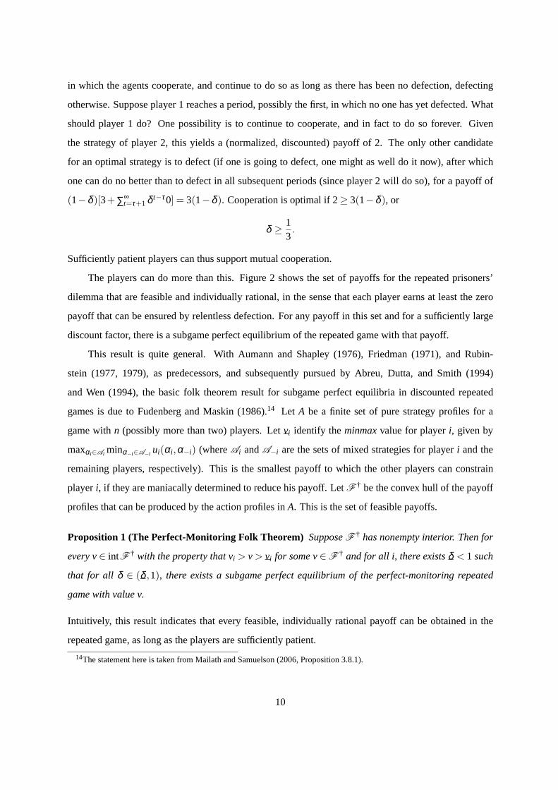
(1−δ )[3+∑∞t=τ+1 δ t−τ0] = 3(1−δ ). Cooperation is optimal if2≥ 3(1−δ ), or
δ ≥ 13.
Sufficiently patient players can thus support mutual cooperation.
The players can do more than this. Figure 2 shows the set of payoffs for the repeated prisoners’
dilemma that are feasible and individually rational, in the sense that each player earns at least the zero
payoff that can be ensured by relentless defection. For any payoff in this set and for a sufficiently large
discount factor, there is a subgame perfect equilibrium of the repeated game with that payoff.
This result is quite general. With Aumann and Shapley (1976), Friedman (1971), and Rubin-
stein (1977, 1979), as predecessors, and subsequently pursued by Abreu, Dutta, and Smith (1994)
and Wen (1994), the basic folk theorem result for subgame perfect equilibria in discounted repeated
games is due to Fudenberg and Maskin (1986).14 Let A be a finite set of pure strategy profiles for a
game withn (possibly more than two) players. Let¯vi identify theminmaxvalue for playeri, given by
maxαi∈Ai minα−i∈A−i ui(αi ,α−i) (whereAi andA−i are the sets of mixed strategies for playeri and the
remaining players, respectively). This is the smallest payoff to which the other players can constrain
playeri, if they are maniacally determined to reduce his payoff. LetF † be the convex hull of the payoff
profiles that can be produced by the action profiles inA. This is the set of feasible payoffs.
Proposition 1 (The Perfect-Monitoring Folk Theorem) SupposeF † has nonempty interior. Then for
everyv∈ intF † with the property thatvi > v >¯vi for somev∈F † and for all i, there exists
¯δ < 1 such
that for all δ ∈ (¯δ ,1), there exists a subgame perfect equilibrium of the perfect-monitoring repeated
game with valuev.
Intuitively, this result indicates that every feasible, individually rational payoff can be obtained in the
repeated game, as long as the players are sufficiently patient.
14The statement here is taken from Mailath and Samuelson (2006, Proposition 3.8.1).
10
2.2 Imperfect Public Monitoring
An important ingredient in the folk theorem for perfect monitoring games is that the players can observe
each others’ behavior.15 For example, this allows them to punish defection in the prisoners’ dilemma.
Moreover, if the threat of punishment creates the proper incentives, then the agents fortuitously never
have to actually do the punishing.
We might expect the players to have quite good information about others’ play, but perhaps not
perfect information. If so, we are interested in games ofimperfectmonitoring. Green and Porter (1984)
and Porter (1983b,a) popularized games of imperfectpublicmonitoring, meaning that the agents observe
noisy signals of play, but all agents observe the same signals.
We first illustrate with the prisoners’ dilemma of Figure 1. We now assume that players cannot
observe their opponent’s actions, instead in each period observing either signal¯y or signal y, gener-
ated according to a probability distribution that depends upon the action profilea taken in that period
according to:
Pr{y | a}=
p, if a = CC,
q, if a = DC or CD
r, if a = DD,
(1)
where0< r < q< p< 1. For example, we might interpret the prisoners’ dilemma as a partnership game
whose random outcome is either a success (y) or failure (¯y).16
Let us first examine the counterpart of the grim trigger strategy for this game of imperfect moni-
toring. Since defection makes the signal¯y more likely, we examine a strategy in which players initially
cooperate, do so as long as the signaly is received, but switch to permanent defection once¯y is received.
For these strategies to constitute an equilibrium, it is again necessary and sufficient that an agent be
15We encountered the importance of good information about previous actions in Section 1.4.16Can’t player 1 figure out what 2 has chosen by looking at the payoffs 1 receives? We assume that player 1’s payoffs are
determined as a function of 1’s actions and the public signal as follows:
y¯y
C (3−p−2q)(p−q) − (p+2q)
(p−q)
D 3(1−r)(q−r) − 3r
(q−r)
The same is true for player 2. This ensures that the distribution of 2’s action, conditional on the public signal and 1’s payoff,
is the same as the distribution conditional on just the public signal, ensuring that payoffs contain no additional information. It
also ensures that the payoffs given in Figure 1 are the expected payoffs as a function of the agents’ actions, so that the players
face a prisoners’ dilemma.
11
willing to cooperate when called upon to do so, or
(1−δ )2+δ pV ≥ (1−δ )3+δqV, (2)
whereV is the expected value of playing the game, given that no one has yet defected. The calculation
recognizes that with probabilityp (if the agent cooperates) orq (if the agent defects), the signaly appears
and the game enters the next period with expected payoffV, while with the complementary probability,
signal¯y appears and subsequent defection brings a zero payoff. We can solveV = (1−δ )2+δ pV for
V =2(1−δ )1−δ p
,
and then insert in (2) to calculate that the proposed strategies are an equilibrium if
δ (3p−2q)≥ 1.
Hence, we have an equilibrium if the players are sufficiently patient and the signals are sufficiently
informative, in the sense thatp must be large enough relative toq. Impatient players or signals that
provide insufficiently clear indications of defection will disrupt the equilibrium.
We thus have some equilibrium cooperation, but with payoffs that are less attractive than those of
the perfect monitoring case. Eventually, the signal¯y will appear, no matter how diligent the agents are
about cooperating, after which these strategies doom them to defection. Indeed, as the players become
increasing patient (δ → 0), the expected payoff from this equilibrium converges to zero, as less and less
importance is attached to the transient string of initial cooperation.
Perhaps we have simply chosen our strategy poorly. Could we do better? Since the difficulty with
grim trigger is that the players eventually end up in a permanent punishment, let us make the punishment
temporary. Suppose that the players initially cooperate and do so after every instance of the signaly. If
they observe signal¯y in a period in which they are supposed to cooperate, they defect for a single period
and then return to cooperation.
It is obvious that the players have no incentive to do anything other than defect when they are
supposed to, since the opponent is then also defecting and nothing can speed the return to cooperation.
These strategies will be an equilibrium if it is optimal to cooperate when called upon to do so. We can
calculate that this incentive constraint is given by
2δ (p−q)≥ 1−δ p−δ 2(1− p)1−δ
.
In the limit, asδ → 1, this becomes3p≥ 2(1+q). Hence, the proposed strategies are again an equilib-
rium if the players are sufficiently patient and the signals sufficiently informative.
12
As the players become increasing patient, the expected payoff from this strategy profile approaches
22− p
.
This is better than the zero payoff of our grim trigger adaptation, but still falls short of the payoff 2 to be
had from persistent mutual cooperation.
These two examples reflect a basic property of equilibria in games of imperfect monitoring: pun-
ishments happen. The only way to create incentives for the players to do anything other than defect is to
ensure that some signals bring lucrative continuation play and others bring bleak continuation play. But
if this is to be the case, unlucky signal realizations will sometimes bring punishments. Moreover, the
players will inflict such punishments even though they know that no one did anything to warrant such a
response. In equilibrium, players who have observed¯y know that everyone has cooperated and that they
were unlucky to have drawn signal¯y, but nonetheless they punish (and indeed would be punished for not
doing so). In essence, players are not punished because they are guilty, but are guilty (or deserving of
punishment) because they are punished. Why would anyone participate in such a crazy equilibrium? It
is not clear that player can choose whether to participate, or can choose an equilibrium if they do partic-
ipate, but it is worth noting that this equilibrium can bring higher expected payoffs than an equilibrium
in which no one is ever punished.
Given the inevitability of punishment, it is natural to conjecture that inefficiency is a general prop-
erty of imperfect monitoring. Against this background, Fudenberg, Levine, and Maskin (1994) produced
a startling result, in the form of a folk theorem for games of imperfect public monitoring. The follow-
ing version of the result is taken from from Mailath and Samuelson (2006, Proposition 9.2.1), with the
understanding that the terms “pairwise full rank” and “individual full rank” are yet undefined:
Proposition 2 (The Public-Monitoring Folk Theorem) SupposeF † has nonempty interior, and all
the pure action profiles yielding the extreme points ofF † have pairwise full rank for all pairs of players.
If the vector of minmax payoffs¯v = (
¯v1, . . . ,
¯vn) is Pareto inefficient and the profileα i that minmaxes
player i has individual full rank for alli, then for allv∈ intF † with vi >¯vi for all i, there exists
¯δ < 1
such that for allδ ∈ (¯δ ,1), v is a subgame-perfect equilibrium payoff.
There are two keys to this result. First, we need the set of feasible payoffs to have an interior.
This ensures that, in response to a signal that is relatively likely when playeri deviates, we can push
continuation payoffs toward payoffs that are worse fori but better for the other players. This allows us to
create incentives without sacrificing efficiency. The second requirement is that the signals be sufficiently
13
informative to give us information not only about whether a deviation has occurred, but also about who
has deviated. This is reflected in the “individual full rank” and “pairwise full rank” conditions in the
theorem. We will leave the statement and discussion of these conditions to Fudenberg, Levine, and
Maskin (1994) and Mailath and Samuelson (2006, Chapter 9)). Intuitively, they ensure that a deviation
from equilibrium play by each playeri has a distinctive effect on the public signals, so that there exists
a signal that is “relatively likely when playeri deviates.” For example, the prisoners’ dilemma with
which we introduced imperfect monitoring in this sectionfails these conditions. Given action profile
CC. the signals can provide information about whether there has been a deviation (i.e.,¯y is more likely if
someone playedD), but no information about who might have deviated. As a result, we are constrained
to inefficiency.
2.3 Private Monitoring
Just as players may not always have precise information about previous play, so may they often not have
precisely the same information. We are then in the realm ofprivatemonitoring.
Suppose we again have the prisoners’ dilemma of Figure 1. Given a choice of actions, let a hypothet-
ical or “latent” signal be drawn from the set{¯y, y} according to the distribution given by (1). However,
instead of assuming that the agents both observe this signal, we use it as a basis for constructing a pair
of private signals.
2.3.1 Conditionally Independent Signals: A First Result
Suppose first that, when signaly is drawn, each playeri independently observes signalyi with probability
1−ζ and signal¯yi with probabilityζ . Things are reversed when signal
¯y is drawn. We refer to this as the
case of conditionally independent monitoring, since, conditioning on the action profile, agenti’s signal
provides no information about agentj ’s signal.
Whenζ is very small, the two players almost certainly receive the same signals. How much dif-
ference could it make that they don’t have exactly the same information? Consider a strategy profile
in which the agents playerCC in the first period, and in which signal¯yi causes agenti to switch to a
punishment phase beginning withD. This seems a promising start on an equilibrium strategy. An agent
makes the signal¯yi more likely by deviatingD, so that attaching punishments to
¯yi should provide the
required incentives to cooperate.
Suppose now that each player adopts such a strategy, that player 1 dutifully choosesC in the first
14
period, and then unluckily draws signal¯y1. Player 1 can then reason, “player 2 has certainly chosen her
equilibrium action ofC (since that is how the equilibrium hypothesis asks me to reason), and has almost
certainly observedy2 (since I playedC, and there is not much noise in the signals), and hence is prepared
to continue with cooperation next period. If I chooseD, I make it very likely that she sees¯y2 and switches
to her punishment phase, to my detriment. If I chooseC again, then there is a good chance we can avoid
the punishment phase altogether, at least for a while.” As a result, player 1 will not enter the punishment
phase, precluding the optimality of the strategy profile. Even the tiniest amount of privateness disrupts
the proposed equilibrium.17
On the strength of this reasoning, initial expectations were that equilibria in repeated games with
private monitoring must be inefficient, and perhaps presented very little prospect for effectively using
intertemporal incentives. This in turn raises the fear that repeated games of public or perfect monitoring
might be a hopelessly special case. As was the case with imperfect public monitoring, these expectations
were displaced by a surprising result, this time from Sekiguchi (1997).
Say that private monitoring isε-perfectif, for each playeri and each action profilea, there is a
signal that playeri receives with probability at least1− ε when action profilea is played.18 Working
with the prisoners’ dilemma, Sekiguchi (1997) showed the following:
Proposition 3 For all η > 0, there existsε > 0 and¯δ < 1 such that for allδ ∈ (
¯δ ,1), if the private
monitoring isε-perfect, then there is a sequential equilibrium in which each playeri’s average payoffs
are within at leastη of ui(C,C).
It is not surprising that the monitoring technology is required to be sufficiently informative (ε small), for
much the same reason that we need the players to be patient. Otherwise, we have no hope of creating
intertemporal incentives.19 The surprise here is the ability to achieve efficiency with private signals, no
matter how close to perfect.
We can provide an indication of the basic technique involved in the equilibrium construction. Sup-
pose that each player mixes in period 1, placing probability1−ξ onC and probabilityξ onD. Suppose
17See Bagwell (1995) for a precursor of this argument and Bhaskar (2005), Guth, Kirchsteiger, and Ritzberger (1998), and
Hurkens (1997) for subsequent discussion.18Notice that for the signals discussed in the opening paragraphs of this section to beε-perfect, not only mustζ be small,
so that each player almost certainly observes the public signal without error, but the distribution given by (1) must approach
perfect monitoring. Sekiguchi’s result requires the monitoring to beε-perfect, but not conditionally independent19For an extreme illustration, consider the completely uninformative case in which each of playeri’s signals appears with
equal probability, independently ofj ’s signals and no matter what the action profile.
15
further thatξ is large relative toε, the measure of noise in the private monitoring. Let playeri continue
with actionC in the second period ifi happened to chooseC in the first period and observed signalyi , and
otherwise leti switch to actionD. Now consider again our previously problematic case, that in whichi
playedC and observed signal¯yi . Playeri can now reason, “I’ve seen signal
¯yi . Either player 2 choseC
and I happened to see the unlikely signal¯yi , or 2 choseD and I received the (then relatively more likely)
signal¯yi . Becauseε is small relative toξ , the latter is more likely. Hence, 2 will enter the punishment
phase next period, and so should I.”
This at least allows the prospect of coordinating punishments. There are many details to be taken
care of in converting this intuition into an equilibrium. In particular, we must ensure that 1 indeed finds
it a best response to enter the punishment, given that 1 thinks 2 is likely but not certain to do so. We must
make sure that we have the indifference conditions required for mixing in the first period. Finally, we
have the problem that this mixing itself introduces some inefficiency. Fortunately, this inefficiency can
be made small asε becomes small, opening the door to an efficiency result.
2.3.2 Belief-Free Equilibria
The equilibrium constructed by Sekiguchi (1997) is abelief-basedequilibrium, in the sense that each
player keeps track of beliefs about the signals the other player has observed. The difficulty is that such
beliefs quickly become quite complicated. We describe here a more recent but all the more surprising
development,belief-freeequilibria, introduced by Piccione (2002), simplified and extended by Ely and
Valimaki (2002)), and characterized by Ely, Horner, and Olszewski (2005).
We continue with our prisoners’ dilemma example, allowing arbitrary private monitoring technolo-
gies. We consider an equilibrium in which each playeri’s strategy is built from four mixtures, that we
refer to asαCyi , αC¯yi , αDyi , αD
¯yi . In each period, playeri choosesC with probabilityαCyi if i choseC and
sawy in the previous period (choosingD with complementary probability); choosesC with probability
αC¯yi if he choseC and saw
¯y; and so on. It is then useful to think of playeri’s strategy as consisting of
four states, one corresponding to each of the mixturesi might choose, and as playeri being in one of
these states in each period, depending upon his experience in the previous period.
The potential difficulty in showing that these strategies are an equilibrium is that each time player
i is called upon to mix,i must be indifferent between the actionsC andD. The payoffs to these actions
depend upon what playerj is doing, again raising the potentially very difficult problem of playeri having
to keep track of beliefs about what playerj has observed and hence is playing. The surprising result is
16
that this is unnecessary. One can choose the various mixtures so that playeri is indifferent betweenC
andD no matter what state playerj is in, and hence no matter whati believes about playerj. Hence,i
can dispense with the need to keep track of beliefs at all, prompting the name “belief-free” equilibrium.
One’s first thought is that the conditions required to support such indifference must be hopelessly
special, often failing and allowing very little control over the payoffs they produce when they are sat-
isfied. To the contrary, it turns out that there are many such equilibria. Indeed, we have a partial folk
theorem. In our prisoners’ dilemma example, any payoff profilev with vi ∈ (0,2) can be achieved as
an equilibrium outcome if the players are sufficiently patient and the monitoring sufficiently close to
perfect.20 Private monitoring thus poses no obstacle to a prisoners’-dilemma folk theorem.
Ely, Horner, and Olszewski (2005) provide a general characterization of the set of belief-free pay-
offs in games with patient players. They find that the prisoners’ dilemma is rather special. In most games
they are not sufficient to prove a folk theorem, even for vanishing noise. However, in the course of this
analysis, Ely, Horner, and Olszewski (2005) show that the basic techniques for working with games of
perfect or public monitoring extend to games of private monitoring.21 Moreover, belief-free behavior
can serve as a point of departure for constructing folk theorems. Matsushima (2004) uses review strate-
gies, familiar from Radner’s (1985) work on repeated principal-agent problems, to extend the belief-free
folk theorem for the prisoners’ dilemma with almost perfect private monitoring to cases in which the
monitoring is quite noisy. Horner and Olszewski (2005) prove a general folk theorem for almost-perfect
private monitoring using profiles that have some of the essential features of belief-free equilibria.
2.3.3 Almost Public Monitoring
Interest in repeated games centers around the ability to use future play to create current incentives. We
thus think of the players as using the history of play to coordinate on a continuation equilibrium. In the
20More complicated strategies allow equilibria to be constructed in which one player receives a payoff larger than 2.21The hallmark of games with perfect monitoring is their recursive structure—each period marks the beginning of a contin-
uation subgame that is identical to the original game. Games of public monitoring have a similar recursive structure, as long as
the players usepublic strategies—strategies in which actions depend only upon the public history of signals, and not players’
private information about their own past actions. (For many purposes, this restriction causes no difficulties—for example, the
public-monitoring folk theorem requires only public strategies—though Kandori and Obara (2003) explore circumstances un-
der which it can be limiting to restrict attention to public strategies). It appears as if the recursive structure has been lost forever
in games of private monitoring. In each period past the first, the players have different information, both about their signals
and their actions, ensuring that the repeated game has no proper subgames at all. However, Ely, Horner, and Olszewski (2005)
show that the recursive techniques of Abreu, Pearce, and Stacchetti (1990) extend to private-monitoring games.
17
prisoners’ dilemma, for example, the players support equilibrium cooperation by using histories featuring
defection as a signal to coordinate on a continuation equilibrium featuring relentless defection.
In the belief-free equilibria of private-monitoring games, this sense of using histories to coordinate
continuation play is lost. Instead of coordinating future play with playerj, playeri gives no thought to
what j might do. Is there any prospect of constructing equilibria in games of private monitoring that have
more of the coordination flavor of equilibria from perfect or public monitoring games?
Mailath and Morris (2002, 2005) examine games ofalmost-publicmonitoring. Return to our pris-
oners’ dilemma example. Once again, we think of an intermediate signal being drawn according to the
the distribution given by (1). Now suppose that if signaly is drawn, with probability1−ζ playersi and
j observeyi and y j , while with probability ζ2 player i observesyi and j observes
¯y j (with the reverse
pattern also having probabilityζ2 ). Similarly, if¯y is drawn, with probability1− ζ player i observes
¯yi
and j observes¯y j . Notice thati’s signal now provides considerable information aboutj ’s, unlike the case
of conditionally independent signals. Asζ → 0, we approach the case of public monitoring.22
Now consider strategies that playC in the first period and switch toD upon observing the signal
¯y. Suppose player 1 cooperates and observes the signal
¯y. Unlike the case of conditionally independent
private monitoring, player 1’s inference is now that player 2 has almost certainly (whenζ is small) also
observed¯y, and is also switching toD. We thus avoid the difficulties that immediately scuttled such
strategies in the case of conditionally independent monitoring.
Ensuring that we have an equilibrium hinges upon showing that players can always be reasonably
confident of where their opponent is in their strategy. Consider first a strategy in which playeri initially
cooperates and does so after any signalyi . After any signal¯yi , player i defects (switching back to
cooperation at the nextyi signal). If the signals are sufficiently informative and the players sufficiently
patient, then this strategy profile is astrict equilibriumunder the imperfect public monitoring scheme
given by (1). The strategies will then also be an equilibrium for private monitoring that is sufficiently
close to being public. The key to this result is that the strategies in question have bounded (in this case,
1-period) recall, meaning that only a finite string of signals is required to identify a player’s action.
This ensures that playeri’s estimate of playerj ’s action depends only on a limited number of signals
and accordingly can never be too far away fromj ’s actual action (given monitoring sufficiently close to
public).
This result is more general. For any strategy profile that has bounded recall and that is a strict equi-
22Unlike the case ofε-perfect monitoring for smallε, there is no presumption here that the limiting public monitoring
distribution be close to perfect monitoring.
18
librium an a game with public monitoring, there is a corresponding strategy profile that is an equilibrium
in the associated private monitoring game, if the monitoring in the latter is sufficiently close to the public
monitoring of the former.
The same result does not hold for strategies with unbounded recall. For example, let playeri initially
cooperate and continue to do so until the first signal¯yi , at which pointi switches to defecting. Defection
continues until the first signal¯yi , at which pointi switches to cooperating, and so on. Hence, we can think
of playeri as having a cooperate state and a defect state, switching whenever¯yi is observed. There are
again conditions under which this strategy is an equilibrium of the public-monitoring game. However,
no matter how close to public monitoring is the private-monitoring game, it is not an equilibrium for the
two players to each choose the counterpart of this strategy under private monitoring. The difficulty is
that the strategy has infinite recall, in the sense that one must know the entire history of signals in order
to identify the strategy’s current state. This ensures that eventually playeri will have virtually no clue as
to player j ’s state, disrupting the equilibrium conditions.
2.3.4 Working with Private Monitoring
Recent years have witnessed surprising progress in working with repeated games of private monitoring,
making it clear that the equilibrium possibilities in such games are richer than initially suspected. Much
now depends upon the interpretation of belief-free equilibria, and in particular upon how one views the
pervasive randomization upon which they are constructed. While mixed strategies are used routinely
in economic models, many economists persist in viewing them uneasily (e.g., Rubinstein (1992)), an
unease that is likely to be heightened by the central role they play in belief-free equilibria. Moreover,
it is not clear whether such equilibria can be purified (Harsanyi (1973)), possibly foreclosing one of the
most popular interpretations of mixtures.23 One the one hand, belief-free equilibria appear to miss the
connection between histories of play and continuation equilibria that is commonly the centerpiece of
work in repeated games. However, the strongest and most complete results for private-monitoring games
have been obtained with belief-free equilibria. It remains to be seen whether belief-free equilibria will
become the standard tool for working with such games, or whether interest will turn to other techniques.
23More specifically, it is not clear if, in general, a belief-free equilibrium can be approximated by any strict equilibrium in
nearby games of incomplete information, where the incomplete information is generated by independently distributed (over
time and players) payoff shocks.
19
2.4 Interpreting The Folk Theorem
The folk theorem asserts that “anything can be an equilibrium.” The only payoffs for which equilibrium
behavior in a repeated game cannot account are obviously uninteresting, and can be so classified without
the help of an elaborate theory, being either infeasible or offering some player less than his minmax
payoff. This result is sometimes viewed as an indictment of the repeated games literature, implying that
game theory has no empirical content. The common way of expressing this is that “a theory that predicts
everything predicts nothing.”
The first point to note in response is that multiple equilibria are common in settings that range far
since this is the set containing the set of subgame-perfect equilibrium payoffs that got us started on the
simplification of the characterization. This must hold for everyλ . Hence, the set of subgame perfect
equilibria must be contained in the intersection of the setsH∗(λ ), for every nonzeroλ ∈ R2.
This provides a tool for studying subgame-perfect equilibrium payoffs, imposing bounds whose
usefulness we’ve seen in examining the public-monitoring prisoners’ dilemma. The more remarkable
result is that, asδ → 1, the set of equilibrium payoffs converges to this intersection (∩λ H∗(λ )). This is a
straightforward recipe for an exact characterization of the set of equilibrium payoffs for patient players.
4 Characterizing Behavior
Theoretical models based on repeated games have been used to examine a variety of economic relation-
ships. This section briefly presents three examples.
25This is consistent with our observation, at the end of Section 2.2, that this game and monitoring technology fail the sufficient
conditions of Proposition 2.26This leaves open the possibility that mixed equilibria may allow symmetric payoffs that are arbitrarily close to efficient,
but a similar argument excludes this possibility as well.
26
4.1 Time Consistency
The idea of time (in)consistency appears regularly in discussion of government policy (e.g., Chari and
Kehoe (1990), Kydland and Prescott (1977), and Ljungqvist and Sargent (2004, Chapter 22)). To fit this
into our repeated-games context, let us think of player 1 is a government. The role of player 2 is filled by
a continuum of consumers. Each player 2 is a negligible portion of the economy, and can hence expect
her current actions to have no effect on future play. Each consumer accordingly chooses a myopic best
response in each period.
In each period, each player 2 is endowed with one unit of a consumption good. The consumer
divides this unit between consumptionc and capital1− c. Capital earns a gross return ofR, so that
the consumer amassesR(1− c) units of capital. The government sets a tax ratet on capital, collecting
revenuetR(1−c) with which it produces a public good. One unit of revenue producesγ > 1 of the public
good. Untaxed capital is consumed. Notice that all of this happens within a period. There are no savings
across periods and the problem of time consistency will arise completely within a period.
The consumer’s utility is given by
c+(1− t)R(1−c)+2√
G, (8)
whereR−1 < γ < RandG is the quantity of public good. The government chooses its tax rates so as to
maximize the consumer’s utility. There is thus no conflict of interest.
Each individual consumer makes a negligible contribution to the government’s tax revenues, and
accordingly treatsG as fixed. The consumer thus choosesc to maximizec+ (1− t)R(1− c). The
consumer’s optimal behavior, as a function of the government’s tax ratet, is then given by:
c(t) =
0 if t < R−1R
1 if t > R−1R .
(9)
If every consumer choosesc, the government’s best response is to choose the tax rate so as to
maximize the consumers’ utility, or
c+(1− t)R(1−c)+2√
γtR(1−c),
where the government recognizes that the quantity of the public good depends upon its tax rate. We can
take a derivative of (8) int and solve to obtain the government’s optimal tax rate as a function ofc, given
by
t(c) =γ
R(1−c). (10)
27
c
t
1
1
R
R 1−
R
γ
A
)(ct
)(tc
B
C
)(tc
)(tc
)(ct
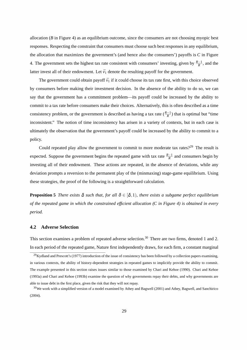
Figure 4: Consumer best responsec(t) as a function of the tax ratet, and government best responset(c)
as a function of the consumptionc.
Figure 4 illustrates the best responses of consumers and the government.27
The efficient outcome calls for consumers to setc = 0. SinceR> 1, investing in capital is produc-
tive, and since the option remains of using the accumulated capital for either consumption or the public
good, this ensures that it is efficient to invest all of the endowment. The optimal tax rate (from (10)) is
t = γR. This gives the allocationB in Figure 4.
It is apparent from Figure 4 that the stage game has a unique Nash equilibrium outcome in which
consumers invest none of their investment (c = 1) and the government tax rate is set sufficiently high as
to make investments suboptimal. OutcomeA in Figure 4 is an example.28 This equilibrium minmaxes
both the consumer and the government. Remarkably, this result arises in a setting where the government
and the consumers have identical utility functions.
There are no circumstances in the repeated game under which we can hope to obtain the efficient
27We omit in Figure 4 the fact that if consumers setc = 1, investing none of their endowment, then the government is
indifferent over all tax rates, since all raise a revenue of zero.28There are other Nash equilibria in which the government sets a tax rate less than one, since the government is indifferent
over all tax rates whenc = 1, but they all involvec = 1.
28
allocation (B in Figure 4) as an equilibrium outcome, since the consumers are not choosing myopic best
responses. Respecting the constraint that consumers must choose such best responses in any equilibrium,
the allocation that maximizes the government’s (and hence also the consumers’) payoffs isC in Figure
4. The government sets the highest tax rate consistent with consumers’ investing, given byR−1R , and the
latter invest all of their endowment. Letv1 denote the resulting payoff for the government.
The government could obtain payoffv1 if it could choose its tax rate first, with this choice observed
by consumers before making their investment decision. In the absence of the ability to do so, we can
say that the government has a commitment problem—its payoff could be increased by the ability to
commit to a tax rate before consumers make their choices. Alternatively, this is often described as a time
consistency problem, or the government is described as having a tax rate (R−1R ) that is optimal but “time
inconsistent.” The notion of time inconsistency has arisen in a variety of contexts, but in each case is
ultimately the observation that the government’s payoff could be increased by the ability to commit to a
policy.
Could repeated play allow the government to commit to more moderate tax rates?29 The result is
expected. Suppose the government begins the repeated game with tax rateR−1R and consumers begin by
investing all of their endowment. These actions are repeated, in the absence of deviations, while any
deviation prompts a reversion to the permanent play of the (minmaxing) stage-game equilibrium. Using
these strategies, the proof of the following is a straightforward calculation.
Proposition 5 There exists¯δ such that, for allδ ∈ [
¯δ ,1), there exists a subgame perfect equilibrium
of the repeated game in which the constrained efficient allocation (C in Figure 4) is obtained in every
period.
4.2 Adverse Selection
This section examines a problem of repeated adverse selection.30 There are two firms, denoted 1 and 2.
In each period of the repeated game, Nature first independently draws, for each firm, a constant marginal
29Kydland and Prescott’s (1977) introduction of the issue of consistency has been followed by a collection papers examining,
in various contexts, the ability of history-dependent strategies in repeated games to implicitly provide the ability to commit.
The example presented in this section raises issues similar to those examined by Chari and Kehoe (1990). Chari and Kehoe
(1993a) and Chari and Kehoe (1993b) examine the question of why governments repay their debts, and why governments are
able to issue debt in the first place, given the risk that they will not repay.30We work with a simplified version of a model examined by Athey and Bagwell (2001) and Athey, Bagwell, and Sanchirico
(2004).
29
cost equal to either¯θ or θ >
¯θ , with the two values being equally likely. The firms then simultaneously
choose prices, drawn fromR+. There is a unit mass of consumers, each potentially buying a single unit
of the good, with a reservation price ofr > θ . A consumer purchases from the firm setting the lower
price if it does not exceedr. Consumers are indifferent between the two firms if the latter set identical
prices, in which case we specify consumer decisions as part of the equilibrium. A firm from whom the
consumers all purchase at pricep, with costθ , earns payoffp−θ .
The stage game has a unique symmetric Nash equilibrium. A firm whose cost level isθ sets price
θ and earns a zero expected profit. A low-cost firm chooses a price according to a distributionF(p) with
support on[ ¯θ+θ
2 , θ ].31 The expected payoff to each firm from this equilibrium is given by14[θ −
¯θ ]. If
r is much larger thanθ , the firms are falling far short of the monopoly profit. An upper bound on the
payoffs in a symmetric-payoff equilibrium arises if both firms set pricer, but with only low-cost firms
(if there is such a firm) selling output, for an expected payoff to each firm of
18(r− θ)+
38(r−
¯θ)≡ v∗.
The repeated game is one of imperfect public monitoring, in the sense that, given a strategy that
attaches different prices to different cost levels, the stage-game outcome reveals only one of these prices.
We are interested in an equilibrium of the repeated game that maximizes the firms’ payoffs, subject to
the constraint that they receive the same payoff.
Proposition 6 For anyη > 0, here exists aδ < 1 such that for allδ ∈ (δ ,1), there exists a pure perfect
equilibrium with payoff at leastv∗− ε for each player.
We present an equilibrium with the desired property. Our candidate strategies for the firms specify
that a high cost firm choose pricer and a low cost firm pricer − ε for some smallε > 0, after any
history featuring no other prices, and that any history featuring any other price prompts play of the stage-
game Nash equilibrium. We also specify that if an out-of-equilibrium price has ever been set, consumers
thereafter split equally between the two firms whenever the latter set identical prices.
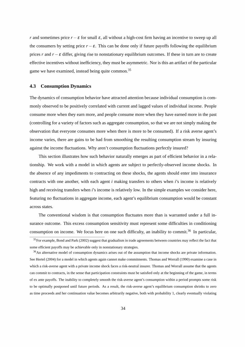
To describe the behavior of consumers in response to equilibrium prices, define three market share
“regimes,”B, I andII , each specifying how consumers behave when the firms both set pricer or both
31It is straightforward that prices aboveθ are vulnerable to being undercut by one’s rival and hence will not appear in
equilibrium, so that high-cost firms must set priceθ . The lower bound on the support of the low-cost firm’s price distribution
must make the firm indifferent between selling with probability 1 at that price and selling with probability12 at priceθ , or
p−¯θ = 1
2(θ −¯θ), giving p = ¯
θ+θ2 .
30
Prices
State r− ε, r− ε r− ε , r r, r− ε r, r
B split 1 2 split
I 1 1 2 1
II 2 1 2 2
Figure 5: Market share regimesB, I , andII , each identifying how the market is split between the two
firms, as a function of their prices.
set pricer−ε. These regimes are shown in Figure 5, where “split” indicates that the market is to be split
equally, and otherwise the indicated firm takes the entire market. Play begins in regimeB, which treats
the firms identically and splits the market whenever they set the same price. RegimeI rewards firm 1
and RegimeII rewards firm 2. The regime shifts toI whenever firm 1 sets pricer and firm 2 sets price
r− ε . The regime shifts toII whenever firm 2 sets pricer and firm 1 sets pricer− ε. Hence, a firm is
rewarded for choosing pricer (while the opponent reports chose pricer− ε) by a presumption that the
firm receives the lion’s share of the market if the two firms set equal prices.
The prescribed actions always allocate the entire market to the low-cost producer, ensuring that the
proposed equilibrium outcome is efficient. The three market share regimes differ in how the market is to
be allocated when the two firms have the same cost level. The payoffs thus shift along a frontier passing
through the equilibrium payoff profile, with a slope of−1. Transitions between states thus correspond
to transfers from one agent to the other. As we have noted in Section 2.2, these are precisely the types of
punishments we should expect if we are to achieve efficient outcomes under imperfect monitoring.
It is a straightforward calculation that expected payoffs from this strategy profile approachv∗ for
each firm (as we makeε small and the firms patient), and that if firms are sufficiently patient, neither will
ever prefer to abandon equilibrium play, triggering permanent play of the stage-game Nash equilibrium,
by setting a price other thanr or r− ε . To complete the argument, we must verify that each firm prefers
to “identify its cost level truthfully,” in the sense that it prefers to make the appropriate choice from the
set{r − ε, r}, given the history of play and its realized cost. We examine the incentive constraints for
the limiting case ofε = 0, establishing that they hold with strict inequality for sufficiently patient firms.
They will continue to hold ifε is sufficiently small.
Let V be the payoff to firm 1 from a continuation game that begins in regimeI (or, equivalently, the
31
value of firm 2 of regimeII ). Conversely, let¯V be the value of firm 2 when beginning in regimeI or firm
1 in regimeII . The requirement that a low-cost firm 1 optimally set pricer− ε rather thanr in regimeI
is
(1−δ )(r−¯θ)+δ (
12¯
V +12
V)≥ (1−δ12(r−
¯θ)+δV.
The requirement that a high cost firm 1 optimally choose pricer in regimeI is:
(1−δ )12(r− θ)+δV ≥ (1−δ )(r− θ)+δ (
12¯
V +12
V).
The requirement that a low-cost firm 2 set pricer− ε in regimeI is
(1−δ )12(r−
¯θ)+δ
¯V ≥ δ (
12¯
V +12
V).
The requirement that a high-cost firm 2 optimally choose pricer in regimeI is
δ (12¯
V +12
V)≥ (1−δ )12(r− θ)+δ
¯V.
RegimeII yields equivalent incentive constraints. LetV be the expected value of a continuation game
beginning in regimeB, which is identical to the two firms. For a low-cost firm to optimally choose price
r− ε, we have
(1−δ )34(r−
¯θ)+δ (
12
V +12¯
V)≥ (1−δ )14(r−
¯θ)+δ (
12
V +12
V).
For a high-cost firm to optimally choose pricer, we need
(1−δ )14(r− θ)+δ (
12
V +12
V)≥ 34(r− θ)+δ (
12
V +12¯
V).
It is then a matter of calculation to show that these constraints hold, and hence that we have an equilib-
rium, for sufficiently largeδ .
This calculation raises three points. First, the further we progressed through the presentation, the
more the language sounded like that of a mechanism design problem, culminating in a collection of
“truth-telling” incentive constraints. This is indicative of themechanism design approachto repeated
games with private-information stage games.32 The mechanism design approach begins by dividing the
prices in this market (or more generally, the actions in a game) into two sets,equilibrium prices and
out-of-equilibriumprices. Out-of-equilibrium prices unambiguously reveal a deviation from equilibrium
32The mechanism design approach is introduced by Athey and Bagwell (2001) and Athey, Bagwell, and Sanchirico (2004),
developed and extended by Miller (2005a,b), and applied by Athey and Miller (2004).
32
play. We can then attach the worst available punishment to these actions, knowing that this punishment
will have no implications for equilibrium payoffs and will deter the deviations (for sufficiently large
discount factors). This allows us to concentrate on equilibrium prices. By viewing continuation payoffs
in the game as transfers, this part of the analysis can be treated as a mechanism design problem, allowing
us to apply the tools of mechanism design theory.
Second, the incentive for firm 1 to set a high price when drawing costθ is that a low price is
punished by a shift to regimeII . The distinguishing feature of regimeII is that indifferent consumers
purchase from firm 2. Firms thus set high prices because consumers punish them for low prices. How
crazy can a model be in which firms collude because their customers punish them for not doing so?
Upon reflection, perhaps not so crazy, because we actually see such arrangements. Firms routinely
advertise that they will “never knowingly be undersold” and that they will “meet any competitor’s price,”
schemes that appear to be popular with consumers. These pricing policies are commonly interpreted as
devices to facilitate collusion by making it less profitable to undercut a collusive price. Consumers who
march into store 1 to demand the lower price they found at store 2 are in fact punishing store 2 for its low
price rather than store 1 for its high price, in the process potentially allowing the firms to collude.
More generally, we return to Section 2.4’s point that we cannot evaluate an equilibrium within
the confines of the model. Instead, we must select an equilibrium as part of constructing the model
of the strategic interaction in question. Depending upon the nature of this interaction, consumers may
well behave in such a way as to support collusion on the part of the firm. This behavior may appear
counterintuitive in the stark confines of the model, while appearing perfectly natural in its actual context.
Third, the firms are ex ante symmetric in our model, and we have focussed attention on maximizing
their payoffs given that they earn the same expected payoffs. It is then natural to suspect that the result-
ing equilibrium would feature symmetric and stationary outcomes—that along the equilibrium path, we
would see the same (symmetric) outcome in each period.33 Instead, we find an equilibrium that makes
important use of nonstationarity and asymmetry along the equilibrium path.34 This is not simply an arti-
fact of the particular equilibrium we have eamined. Efficiency requires that the firms sometimes set price
33We cannot expect the stronger version of stationarity that would require the same actions after every history, both in
and out of equilibrium. Instead, we expect that deviations from equilibrium will trigger punishments. For example, the only
equilibrium in the repeated prisoners’ dilemma satisfying this stronger stationarity property is one in which players defect in
every period, while an equilibrium in which the cooperate in every period, with deviations punished by subsequent defection,
features outcomes that are stationary along the equilibrium path.34The asymmetry is not simply ex post, in the sense that firms with different cost realizations are treated differently, but ex
ante, in the sense that the firms fare differently conditioned on cost realizations, depending upon the history of play.
33
r and sometimes pricer− ε for smallε, all without a high-cost firm having an incentive to sweep up all
the consumers by setting pricer− ε . This can be done only if future payoffs following the equilibrium
pricesr andr− ε differ, giving rise to nonstationary equilibrium outcomes. If these in turn are to create
effective incentives without inefficiency, they must be asymmetric. Nor is this an artifact of the particular
game we have examined, instead being quite common.35
4.3 Consumption Dynamics
The dynamics of consumption behavior have attracted attention because individual consumption is com-
monly observed to be positively correlated with current and lagged values of individual income. People
consume more when they earn more, and people consume more when they have earned more in the past
(controlling for a variety of factors such as aggregate consumption, so that we are not simply making the
observation that everyone consumes more when there is more to be consumed). If a risk averse agent’s
income varies, there are gains to be had from smoothing the resulting consumption stream by insuring
against the income fluctuations. Why aren’t consumption fluctuations perfectly insured?
This section illustrates how such behavior naturally emerges as part of efficient behavior in a rela-
tionship. We work with a model in which agents are subject to perfectly-observed income shocks. In
the absence of any impediments to contracting on these shocks, the agents should enter into insurance
contracts with one another, with each agenti making transfers to others wheni’s income is relatively
high and receiving transfers wheni’s income is relatively low. In the simple examples we consider here,
featuring no fluctuations in aggregate income, each agent’s equilibrium consumption would be constant
across states.
The conventional wisdom is that consumption fluctuates more than is warranted under a full in-
surance outcome. This excess consumption sensitivity must represent some difficulties in conditioning
consumption on income. We focus here on one such difficulty, an inability to commit.36 In particular,
35For example, Bond and Park (2002) suggest that gradualism in trade agreements between countries may reflect the fact that
some efficient payoffs may be achievable only in nonstationary strategies.36An alternative model of consumption dynamics arises out of the assumption that income shocks are private information.
See Hertel (2004) for a model in which agents again cannot make commitments. Thomas and Worrall (1990) examine a case in
which a risk-averse agent with a private income shock faces a risk-neutral insurer. Thomas and Worrall assume that the agents
can commit to contracts, in the sense that participation constraints must be satisfied only at the beginning of the game, in terms
of ex ante payoffs. The inability to completely smooth the risk-averse agent’s consumption within a period prompts some risk
to be optimally postponed until future periods. As a result, the risk-averse agent’s equilibrium consumption shrinks to zero
as time proceeds and her continuation value becomes arbitrarily negative, both with probability 1, clearly eventually violating
34
in each period, and after observing the current state, each agent is free to abandon the current insurance
contract.37 As a result, any dependence of current behavior on current income must satisfy incentive
constraints. The dynamics of consumption and income will arise out of this restriction.
The stage game features two consumers, 1 and 2.38 There is a single consumption good. A random
draw first determines the players’ endowments of the consumption good to be given by one of three
possibilities:
Endowment Probability
Endowmente(1) (y,¯y) 1
3
Endowmente(m)(
12, 1
2
)13
Endowmente(2) (¯y, y) 1
3,
where y ∈ (12,1]. After observing the endowment, players 1 and 2 simultaneously transfer nonnega-
tive quantities of the consumption good to one another, and then consume the resulting net quantities,
evaluated according to the utility functionu(·). The functionu is strictly increasing and strictly concave.
This stage game obviously has a unique Nash equilibrium outcome in which no transfers are made.
Because the consumers are risk averse, this outcome is inefficient. Each agent earns his minmax value
under this equilibrium.
Suppose now that the consumers are infinitely-lived, playing the game in each periodt = 0,1, . . ..
The endowment draws are independent across periods. Players discount at the common rateδ . If the
discount factor is high enough, then there exists a full-insurance equilibrium in which each player’s
participation constraints in the continuation game. Extensions of this model are examined by Atkeson and Lucas, Jr. (1992) (to
a general equilibrium setting) and Atkeson and Lucas, Jr. (1995) (to study unemployment insurance). Wang (1995) shows that
if utility is bounded below, then (obviously) continuation utilities cannot be come arbitrarily negative, and (more importantly)
consumption does not shrink to zero with probability one, since then the accumulation of utility at the lower bound would
preclude the creation of incentives. Ljungqvist and Sargent (2004, Chapter 19) provide a useful discussion.37Ljungqvist and Sargent (2004, Chapter 19) examine a variation on this model in which one side of an insurance contract
can be bound to the contract, while the other is free to abandon the contract at any time. We might interpret this as a case
in which an insurance company can commit to insurance policies with its customers, who can terminate their policies at will.
Bond (2003), Ray (2002) and Thomas and Worrall (1994) similarly examine models in which a principal can commit to a
contract but the agent cannot. We follow Kocherlakota (1996), Ljungqvist and Sargent (2004, Chapter 20) and Thomas and
Worrall (1988) in examining a model in which either party to an insurance contract has the ability to abandon the contract at
will. This might be interpreted as a case in which agents must insure one another.38We draw here on a model of Kocherlakota (1996), discussed by Ljungqvist and Sargent (2004, Chapters 19–20). Ligon,
Thomas, and Worrall (2002) and Thomas and Worrall (1988) present related models. See Koeppl (2003) for a qualification of
Kocherlakota (1996).
35
consumption in each period is independent of the endowment and the history of play. The transfers
required to achieve such consumption are enforced by a switch to the stage-game Nash equilibrium (i.e.,
to mutual minmaxing) should they fail to be made.
Suppose thatδ falls short of¯δ , so that full insurance is impossible, but is large enough that some
nontrivial equilibria exist. We will examine the efficient, symmetric-payoff equilibrium for this case.
We can construct a first candidate for such an equilibrium by assuming that whenever endowmente(i) is
received, agenti transfersε to agentj. Any failure to do so triggers permanent play of the stage-game
Nash equilibrium. We chooseε as large as possible, namely to satisfy
(1−δ )u(y− ε)+δ13
(u(y− ε)+u
(12
)+u(
¯y+ ε)
)= (1−δ )u(y)+δ
¯v.
This is the incentive constraint that an agent having drawn a high endowment be willing to transferε and
continue with equilibrium play rather than pocketing the relatively favorable endowment and switching
to the stage-game Nash equilibrium. Given our assumption that the discount factor is large enough to
support more than the autarky equilibrium, but too small to support full insurance, this equation is solved
by someε ∈ (0, y− 12). This equilibrium leaves consumption untouched in endowmente(m), while
smoothing consumption i endowmentse(1) ande(2). We refer to this equilibrium asσ .
This equilibrium provides some insurance, but we can provide more. Let us separate ex ante histo-
ries into two categories, category 1 and category 2. A history is in categoryi if agenti is the most recent
one to have drawn a high endowment. Now fixζ > 0, and let the strategy profile prescribe consumption
(12 + ζ , 1
2 − ζ ) whenever the agents find themselves facing endowmente(m) after a category-1 history
and consumption(12−ζ , 1
2 +ζ ) when facing endowmente(m) after a category-2 history. In essence, we
are using consumption in endowmente(m) to reward the last agent who has had a large endowment and
transferred part of it to the other agent.
This modification of profileσ has two effects. We are introducing risk in endowmente(m), but with
a second-order effect on total expected payoffs (whenζ is small). However, because we now allocate
endowment-e(m) consumption in order to reward the last agent to make a transfer, this adjustment gives a
first-order increase in the expected continuation payoff to agenti after a history of categoryi. This relaxes
the incentive constraints facing agents when drawing endowmentse(1) ande(2). We can thus couple
the increase inζ with an increase inε, where the latter is calculated to restore equality in the incentive
constraints in endowmentse(1) ande(2), thereby allowing more insurance in endowmentse(1) ande(2).
The increased volatility of consumption in endowmente(m) thus buys reduced volatility in endowments
e(1) ande(2), allowing a first-order gain on the latter at a second-order cost on the former.
36
1,ec
22 ,ec
)1(e
)1(c
)(me
)( 2mc
)2(c
)2(e
)( 1mc
Figure 6: Illustration of the three endowmentse(1), e(m) ande(2), as well as four consumption profiles
c(1), c(m1), c(m2) andc(2), for the efficient, symmetric equilibrium. Consumption bundlec(mi) follows
a history in which endowmente(m) has been drawn, and the last endowment other thane(m) to be drawn
was endowmente(i).
Figure 6 illustrates the resulting consumption pattern. Because profileσ was an equilibrium, this
new profile is also an equilibrium for sufficiently smallζ .39 Choosingζ to be either the largest value
for which this profile is an equilibrium or the value for whichy− ε− 12 +ζ (in which casec(i) = c(mi)
in Figure 6), whichever is smaller, gives us the equilibrium we seek. As in Section 4.2, we have a
symmetric-payoff equilibrium that is not stationary. Current consumption depends upon whether the
history is in category 1 or category 2, in addition to the realization of the current endowment. Intu-
itively, we are now spreading risk across time as well as states within a period, exchanging a relatively
large transfer from a high-endowment agent for a relatively lucrative continuation payoff. In terms of
consumption dynamics, agents with high endowments in their history are now more likely to have high
39The essential observation here is that, underσ , the expected continuation payoff conditional on statem exceeds that of
the repeated play of the Nash equilibrium, introducing slack into the incentive constraints for making transfers in statem that
allows the new equilibrium to support small transfers.
37
h `
H 2,3 0,2
L 3,0 1,1
Figure 7: The product choice game
current consumption.
5 Reputations
It is common to speak of people, firms, governments, and other institutions as having reputations. The
idea of a reputation typically carries some connotation of foregoing an opportunity for short-terms
gains—perhaps by providing high quality instead of shoddier but cheaper merchandize, exerting ef-
fort instead of shirking, behaving honestly rather than opportunistically—even though the immediate
incentives for doing so are not compelling. The rewards for doing so are viewed as arising from links
between current actions and future expectations about one’s behavior. The concept of a reputation thus
fits naturally into a study of relationships.
We will discuss reputations in the context of the “product choice” game shown in Figure 7. We
think of player 1 as a firm who can produce high quality (H) or low quality (L). Player 2 is a consumer
who simultaneously purchases either a high-cost product from the firm (h) or a low-cost product (). The
consumer prefers to buy the expensive product if the firm is providing high quality, and the low-cost
product otherwise. For example, the consumer may prefer dinner with all the trimmings at a fine restau-
rant but a sandwich at the local diner. A patient may prefer heart surgery from a competent physician
but a herbal remedy from a quack. The firm finds high quality expensive and so always earns a higher
payoff from low quality, but prefers that the consumer choose the high cost option. The stage game has
a unique Nash equilibrium in whichL` is played, for payoffs(1,1).
There are two approaches to thinking about reputations. The “equilibrium interpretation” approach
selects an equilibrium of the repeated game and then interprets various of its features in reputation terms.
For example, when the players are sufficiently patient, there is an equilibrium in the repeated product-
choice game in whichHh is played in every period, with any deviations from such play prompting a
switch to (permanent) play of the stage-game equilibriumL`. We might then refer to the firm as main-
taining a reputation for high quality along the equilibrium path, and any deviation as having destroyed
38
this reputation.40 However, there is no necessary link between past behavior and expectations about fu-
ture behavior in such models. For example, there remains an equilibrium in whichL` is played in every
period, and it remains an equilibrium to continue with such behavior even if player 1 desperately tries
to build a reputation by playingH in the first thousand periods. The idea of a reputation is helpful in
keeping track of the behavior in the selected equilibrium, but adds nothing formal to the analysis.
The “adverse selection” approach to reputations, considered here, rests upon the introduction of
incomplete information concerning players’ characteristics. For example, suppose there is some small
probability that player 1 in the product choice game is a commitment type who always playsH, otherwise
being the normal type specified by the stage game. This incomplete information is a mechanism for
creating a necessary link between past play and expected future behavior. In particular, there is no longer
an equilibrium of the repeated product-choice game in which the normal type of player 1 and player
2 invariably chooseL`. Given such a candidate equilibrium, the normal type would chooseH in the
first period, leading player 2 to conclude she was facing the commitment type and hence leading to
subsequent play ofHh. Results in the adverse selection approach consist of restrictions on the set of
equilibria rather than statements about a particular equilibrium.
5.1 Short-Run Opponents
Our examination of the adverse selection approach to reputations begins with a setting in which player
1 is a long-run player, who appears in every period of the infinitely-repeated game. The role of player 2
is filled by a succession of short-run players, each of whom participates in the market for only a single
period. For example, a new customer may come to the firm every period. As a result, each player 2
chooses a myopic best response to player 1’s behavior.
5.1.1 Perfect Monitoring
Suppose first that actions are perfectly monitored.41 There are two possible types of player 1, a “normal”
type whose payoffs are given by Figure 7 and a “Stackelberg” type who always playsH. The game begins
with a draw of player 1’s type, revealed only to player 1, and perhaps attaching very high probability to
player 1 being normal.
40For examples of this approach, see Barro and Gordon (1983), Canzoneri (1985), Ljungqvist and Sargent (2004, Chapter
22), and Rob and Fishman (2005).41The basic result is from Fudenberg and Levine (1989). Celentani and Pesendorfer (1996) present an analogous result for
dynamic games. Fudenberg and Levine (1992) extend the argument to imperfect monitoring.
39
In general, let
v∗1 = maxa1
minα2∈B(a1)
u1(a1,α2) ,
whereB(a1) is the set of player-2 myopic best replies toa1. This is player 1’s pure Stackelberg payoff,
identifying the payoff player 1 could earn in the stage game if 1 could publicly choose a pure action before
2 chooses, with 2 then choosing a best response. Leta∗1 denote the accompanying pure “Stackelberg”
action. In the product choice game, this payoff is 2, secured by choosing actionH. Let µ be the prior
probability attached to the Stackelberg type. We have:
Proposition 7 For any probabilityµ > 0 and for anyε > 0, there exists a¯δ < 1 such that for any
δ ∈ (¯δ ,1), the payoff to the normal type of player 1 in any Nash equilibrium of the repeated game is at
leastv∗1− ε.
To see what lies behind this result, fix an equilibrium of the game and consider player 1’s options.
One possibility is to playa∗1 in every period. The key step to the reputation result describes the conse-
quences of such play:
Lemma 1 For anyη > 0, there is a numbern(η) such that if the normal type of player 1 choosesa∗1 in
every period, the number of periods in which player 2 can attach probability less than1−η to player 1
choosinga∗1 is less thann(η).
Thus, if player2 observes ever-longer strings of actiona∗1, then eventually player2 must come
to expect actiona∗1 to be played with high probability. In particular, suppose we reach a periodt in
which player 1 has hitherto played the Stackelberg action and player 2’s current expectation is that the
Stackelberg action neednotappear. This can only happen if equilibrium play attaches some probability to
the event that player 1 is the normal type and will not play the Stackelberg action. But then Bayes’ rule
ensures that observing the Stackelberg action in periodt results in a posterior that must put increased
weight on the Stackelberg type. As a result, the probability that player 2 attaches to seeing actiona∗1
marches upward, and player 2 must eventually believe either that she is almost certainly facing the
Stackelberg type or facing a normal type who plays like the Stackelberg type. Either way, player 2 must
expect to see the Stackelberg action.
This characterization of beliefs allows us to establish the lower bound on player 1’s equilibrium
payoffs. Let the normal type of player 1 choosea∗1 in every period. After some finite number of periods,
player 2 must believe thata∗1 is sufficiently likely as to play a best response, giving player 1 the payoff
40
v∗1. Player 1 may earn lower payoffs in the early periods before 2 expectsa∗1, but these early periods are
insignificant if player 1 is sufficiently patient. This ensures a repeated-game payoff arbitrarily close tov∗1
for a patient player 1. Notice that continually playinga∗1 maynotbe optimal for player 1, but 1’s optimal
strategy must give a payoff at least this large. In the case of the product choice game, continually playing
H suffices for player 2 to eventually always playh, for a payoff close to 2.
5.1.2 Imperfect Monitoring
With some additional technical complication, a stronger result applies to games of imperfect monitoring
(cf. FudenbergLevine92). For example, suppose that when the product choice game is played, player 2
observes not player 1’s actions, but a signal from the set{¯y, y}, with probabilities
ρ(y | a) =
p, if a1 = H,
q, if a1 = L,
(11)
where0 < q < p < 1. Player 2’s inferences about player 1’s behavior are now clouded by the imperfect
monitoring. The arguments behind Lemma 1 are accordingly replaced by conceptually similar proba-
bilistic arguments (e.g., Sorin (1999)) reflecting the randomness in the monitoring process. If player
1 invariably playsa1, player 2’s expectation ofa1 must increase on average, and she eventually must
play a best response toa∗1 with very high probability. This suffices to ensure a patient player 1 a payoff
arbitrarily close to 2 in the product choice game.
The same techniques that allow us to work with imperfect monitoring allow us to extend the results
to commitment types who play mixed actions, in games of either perfect or imperfect monitoring, in the
process strengthening the reputation result.42 We illustrate with the product choice game, though the
result is general. Player 1 would like player 2 to chooseh. It suffices for this for player 1 be (known to
be) committed toH, but there is a sense in which this is more of an investment in high quality than is
required. It would suffice for 2 to findh a best response that player 1 chooseH with probability just over
12. The reputation argument ensures that, if the commitment type of player 1 chooses such a mixture, the
(patient, normal) player 1 must receive a payoff in any equilibrium of the repeated game that is arbitrarily
close to that from being known to be committed to such a mixture, in this case52. This is all the more
remarkable in light of the fact that, in the case of imperfect monitoring (as in (11)) and no uncertainty
42Because player 2 observes only the realized actions of player 1 and not the underlying mixture, perfectly-monitored oppo-
nents who play mixed actions present inference problems similar to those of imperfectly monitored opponents.
41
about player 1’s type, an argument analogous to that applied to the prisoners’ dilemma in Section 3.2
allows us to conclude that player 1’s payoff is bounded above by
2− 1− pp−q
,
while in the case of perfect monitoring player 1’s type is bounded above by 2 (Mailath and Samuelson
(2006, Section 2.7.2)). The adverse-selection-based reputation thus not only pushes player 1 to the top
of the set of equilibrium payoffs, but expands the set itself.
This discussion may leave the impression that reputation arguments depend critically upon having
just the right commitment type in the model, and perhaps on having only that type, or having that type
be sufficiently likely. None of these is the case. The arguments extend to the case in which player 1 may
be one of an infinite number of possible types, which may not include the pure Stackelberg type. The
bound on player 1’s payoff is then given by allowing him to “choose” from the set of possible types the
one to whose behavior it would be most profitable to commit, regardless of the how likely are the various
types. The arguments further extend to the case in which there is (sufficiently small) uncertainty about
player 2’s type.
5.1.3 Temporary Reputations
Cripps, Mailath, and Samuelson (2004b) establish conditions under which player 1 will eventually spend
his reputation. Under fairly general conditions, player 2 must eventually learn player 1’s type, with play
converging to an equilibrium of the complete-information game defined by player 1’s type.43 In the
product-choice game, for example, reputation effects may constrain player 1’s ex ante payoff to be very
close to52, but his continuation payoff is eventually less 2.
To build intuition for this result, suppose that player 1 may be either a normal or Stackelberg type,
and we have a candidate equilibrium in which player 2 does not learn player 1’s type. Then player 2
must expect Stackelberg-type behavior from both types of player 1. Otherwise, she would eventually
get enough information, even under imperfect monitoring, to sort out which type of player she faced.44
Player 2, being a short-run player, will then play a best response to the Stackelberg type. But then the nor-
mal type of player 1 has an incentive to deviate from the Stackelberg behavior, potentially contradicting
player 2’s belief that player 1 will exhibit Stackelberg behavior.45
43Jackson and Kalai (1999) examine another sense in which reputations are temporary, in finitely-repeated games.44An assumption plays a role here, namely that the signals are sufficiently informative that player 2 can distinguish different
actions of player 1, given sufficient observations.45Three assumptions are embedded here. First, that the structure of the game and signals is such that player 1 knows player
42
This is a limiting result, describing beliefs and behavior in the possibly very distant future. While
the short-run properties of equilibria are interesting, we believe that the long-run equilibrium properties
are also relevant in many situations. For example, an analyst may not know the age of the relationship
to which the model is to be applied. We sometimes observe strategic interactions from a well-defined
beginning, but we also often encounter on-going interactions whose beginnings are difficult to identify.
Long-run equilibrium properties may be an important guide to behavior in the latter cases. Alternatively,
one might take the view of a social planner who is concerned with the continuation payoffs of the long-
run player and with the fate of all short-run players, even those in the distant future. Our analysis
also suggests that the short-run players may have definite preferences as to where they appear in the
queue of short-run players, offering a new perspective on the incentives created by repeated games.
Finally, interest often centers on thesteady statesof models with incomplete information, again directing
attention to long-run properties.
We view our results as suggesting that a model oflong-run reputations should incorporate some
mechanism by which the uncertainty about types is continually replenished. For example, Holmstrom
(1982), Cole, Dow, and English (1995), Mailath and Samuelson (2001), and Phelan (2005) assume that
the type of the long-run player is governed by a stochastic process rather than being determined once
and for all at the beginning of the game. In such a situation, reputations can indeed have long-run
implications. We return to this in Section 5.4.
How do we reconcile the finding that reputations are temporary with the fact that reputations impose
nontrivial bounds on ex ante payoffs? The answer lies in the “eventually” aspect of our result. There may
well be a long period of time during which player 2 is uncertain of player 1’s type, and in which play does
not resemble an equilibrium of the complete-information game. The length of this period will depend
upon the discount factor, being longer for larger discount factors, and in general being long enough to
have a significant effect on player 1’s payoffs. Eventually, however, such behavior must give way to a
regime in which player 2 is (correctly) convinced of player 1’s type.
We thus have an order of limits calculation. For any prior probabilityµ that the long run player
2’s belief, and hence knows that there is a profitable deviation. Cripps, Mailath, and Samuelson (2004a) relax this assumption.
Second, that the normal player 1 does not find Stackelberg behavior a best response to player 2’s (best response to Stackelberg)
behavior. For example, there would be no difficulty in player 1 maintaining a reputation in the product choice game for being a
commitment type who always playedL—let the equilibrium simply specify(L, `) in every period, regardless of history. Third,
that the monitoring is imperfect, ensuring that the normal player 1’s deviation cannot be deterred by a sufficiently draconian
punishment.
43
is the commitment type and for anyε, there is a discount factor¯δ sufficiently large that player 1’s
expected payoff is withinε of his Stackelberg payoff. This holds no matter how smallµ. As a result,
it is tempting to think that, even as the game is played and the posterior probability of the commitment
type falls, we should be able to choose a period, think of it as the beginning of the game, and apply
the standard reputation argument to conclude that uncertainty about player 1’s type still has a significant
effect. However, for any fixed¯δ and in any equilibrium, there is a time at which the posterior probability
attached to the commitment type has dropped belowµ, becoming too small (relative to¯δ ) for reputation
effects to operate. We are then on the path to completely revealing player 1’s type.
5.2 Two (Asymmetric) Long-Run Players
Section 5.1 examined a model in which player 1, the reputation builder, faced short-run opponents. In
many reputation settings, such as a firm facing a succession of consumers, this seems quite natural. But
what if both players are long-run?
Let player 1 and 2 both be long run players, with (possibly different) discount factorsδ1 andδ2. We
assume that player 1 may be either a normal or a Stackelberg player and ask whether the normal player
1 can exploit this uncertainty to impose a lower bound on his payoff in the repeated game.
Consider the product choice game. We can again proceed by arguing that, if player 2 always ob-
serves actionH, player 2 must eventually belief the continued play ofH is quite likely. This suffices to
ensure ashort-runplayer 2 playsh, the second important piece in the argument. However, the same is
not necessarily the case for a long-run player 2. In particular, 2’s expectation thatH will very likely be
played in the future is consistent with 2 attaching probability to player 1 being an normal type whose
strategy calls for actionH, a Stackelberg type committed toH, and a “punishment” type who playsH
until the first time 2 playsh, after which the punishment type playsL. The latter type is of no concern
to a short-run player 2, but if a long-run player 2 thinks this latter type sufficiently likely (a belief that
continued observations ofH will do nothing to dispel), 2 will play . We thus cannot simply transfer the
previous argument to the case of two long-run players without imposing some additional structure on the
problem.46
46The simplicity of the product choice game requires that we work with a punishment type whose behavior may appear
counterintuitive or contrived. There is in general no obvious way of avoiding this difficulty by restricting attention to a set of
“plausible” commitment types.
44
5.2.1 Conflicting Interests
We begin with a result from Schmidt (1993). Letv∗1 anda∗1 again be the Stackelberg payoff and action
for player 1. We say that the stage game hasconflicting interestsif
maxα2∈A2
u2(a∗1,α2) = minα1∈A1
maxα2∈A2
u2(α1,α2).
Hence, player 2’s best response to player 1’s Stackelberg action minmaxes player 2.
We then have:
Proposition 8 Let the stage game be one of conflicting interests. Then for anyδ2 < 1 andε > 0, there
exists aδ < 1 such that for allδ ∈ (δ 1,1), the expected payoff of the normal type of player 1 is at least
v∗1− ε.
As expected, the basic tool in the argument is to note that when facing a steady stream ofa∗1, player
2 must eventually come to expect the Stackelberg action. The argument that a long-run player 2 will then
play a best response toa∗1 exploits the fact that this best response minmaxes player 2 (given conflicting
interests), which in turn must be better than 2’s payoff from any other response. We then note that there
are no punishments worse for player 2 than being minmaxed, and hence nothing that can induce player
2 to consistentlynot play a best response toa∗1. This allows a sufficiently patient player 1 to be assured
a payoff close to the Stackelberg payoff.
Notice that the argument requires an asymmetry in discount factors, with player 2’s discount factor
being fixed and player 1’s allowed to approach 1. Player 2’s discount factor plays a role in imposing a
bound on the number of times 2 can fail to play a best response toa∗1. We must then have the freedom
to let player 1’s discount factor increase, to ensure that these periods have an insignificant effect on 1’s
payoff.
What sorts of games exhibit conflicting interests? The prisoners’ dilemma does, but the reputation
result is of no interest here, since player 1’s Stackelberg type always defects and the result ensures
player 1 a payoff of at least 0. The product choice game does not exhibit conflicting interests, and so is
not covered by the result. The chain-store game (Figure 8) satisfies conflicting interests, and the result
implies that player 1 (the incumbent) can earn a payoff arbitrarily close to that to be had from being
committed to fighting entry.
Is there anything we can do to expand the result beyond games of conflicting interests? Cripps,
Schmidt, and Thomas (1996) show that in the absence of conflicting interests, a sufficiently patient player
45
Enter Out
A 2,2 5,0
F −1,−1 5,0
L R
T 0,0 3,1
B 1,3 0,0
Figure 8: Chain store (left) and battle of the sexes game.
1 can be assured a payoff arbitrarily close to that which arises if player 1 commits to an action and player
2 chooses the response that is worst for player 1, conditional on 2 earning at least her minmax payoff.
In the battle of the sexes game, shown in Figure 8 (and which does not have conflicting interests), the
minmax utilities for the two players are(34, 3
4). Suppose that with positive probability, player 1 is thought
to be the Stackelberg type who always playsT. The set of responses toT in which player 2 receives at
least her minmax utility is the set of actions that place at least probability34 on R, ensuring player 1 a
payoff of 94. Hence, the normal player 1, if sufficiently patient and for any player-2 discount factor, must
receive a payoff arbitrarily close to94.47
5.2.2 Imperfect Monitoring
Celentani, Fudenberg, Levine, and Pesendorfer (1996) show that reputations can be more effective in
games of imperfect monitoring. As we have seen, the difficulty in establishing a reputation when facing
a long-run player 2 is that consistently playing like the commitment type will lead player 2 to expect such
behavior on the equilibrium path, but imposes few restrictions on what 2 can believe about play off the
equilibrium path.48 Celentani, Fudenberg, Levine, and Pesendorfer (1996) note that the sharp distinction
between being on and off the equilibrium path disappears in games of imperfect monitoring. Player 2
should then have ample opportunity to become well acquainted with all of player 1’s behavior, including
any punishment possibilities. They exploit this insight to show that, without requiring conflicting inter-
ests, for any player-1 discount factorδ2 andε > 0, there is a¯δ1 such that for allδ1 ∈ (
¯δ1,1), the normal
type of player 1 earns at leastv∗1−ε in every Nash equilibrium of the repeated game. Indeed, by allowing
more sophisticated commitment types, they show that player 1 can be assured a payoff arbitrarily close to
the largest stage-game payoff consistent with individual rationality for player 2, providing the strongest
47In the product choice game,` ensures 2 her minmax payoff no matter what 1 chooses, and is always the worst action for
player 1. The reputation result thus places a lower bound on 1’s payoff that is no higher than can be earned when 2 always
chooses , and hence imposes no restrictions in this case.48Recall that this is not a difficulty in games of conflicting interests because player 2’s payoff along the equilibrium path is
sufficiently low that she has nothing to fear in being pushed off the path.
46
possible reputation result.
5.2.3 Commitment Types who Punish
Evans and Thomas (1997) (see also Evans and Thomas (2001)) take an alternative approach to player
2’s concerns about out-of-equilibrium punishments. Suppose we have a commitment type who punishes
player 2 fornot playing a best response to the Stackelberg action. In the product-choice game, for
example, suppose that a commitment type playsL once, the first time player 2 fails to chooseh; playsL
twice, the next time; and so on. Eventually, player 2 faces arbitrarily long punishments for not playingh.
Now let the normal player 1 mimic this behavior. For familiar reasons, player 2 must come to expect such
play, and must choose a best response. In the product choice game, this ensures that 2 will eventually
playh, ensuring a patient (normal) player 1 a payoff close to 2. In general, by choosing the commitment
type carefully, we again have the result that player 1 can be assured a payoff arbitrarily close to the
largest stage-game payoff consistent with individual rationality for player 2. This is once more a strong
result, one that does not require imperfect monitoring. This argument does require somewhat more
active commitment types than those appearing in many reputation results. No longer does it suffice for a
commitment type to simply play the action for which player 1 would like to develop a reputation, such
asH in the product choice game. Instead, the commitment type must play an active role in “teaching”
player 2 to play a best response to this action.
5.2.4 Reputations with Long-Run Opponents
The message that emerges from these results is that reputations can be effective against long-run oppo-
nents, but that the conditions for reputation building become more stringent than required for short-run
opponents. Once again, the arguments do not require thatonly the right commitment types be present,
or that the various commitment types appear in the right proportions, or that uncertainty be limited to
only one player. However, if the results are to apply to a general class of games, then we must have ei-
ther imperfect monitoring or relatively sophisticated commitment types. One of missing elements in the
study of reputations is a theory of commitment types that would provide some guidance as to what sort
of uncertainty about types captures the intuitive links between current behavior and future expectations
that lie at the heart of a reputation.
Cripps, Mailath, and Samuelson (2004a) extend the “temporary reputations” result of Cripps, Mailath,
and Samuelson (2004b) to games with two long-run players, so that the ex ante and asymptotic implica-
47
tions of reputation models can be quite different. We again see that an assessment of reputation results
must depend upon the setting for which the model is intended.
5.3 Two (Symmetric) Long-Run Players
Sections 5.1 and 5.2 have examined reputations in games where player 2 is a short-run player, and then
in which player 2 is a long-run player but not as patient as player 1. What if both are long run players
and equally patient, orδ1 = δ2 > 1?49
Notice first that some asymmetry must be involved in a reputation result. The essence of a reputation
result is a lower bound on the reputation builder’s payoff, with particular emphasis on the cases in which
this lower bound is close to a suitably defined “Stackelberg” payoff. Both players cannot earn nearly
their Stackelberg payoff in the battle of the sexes (Figure 8), for example, since payoffs near(3,3) are
not feasible. We can then hope only for sufficient conditions for one player to develop such a reputation.
But then we have no hope for such conditions in a perfectly symmetric game, with nothing to distinguish
one of the players as the potential reputation builder.50
In moving from a short-run player 2 through a long-run but less patient player 2 to two long-run and
equally patient players, we have wrung all of the asymmetry out of the players’ discounting. We must
accordingly look for asymmetries in the structure of the game. Two results are available.51
Suppose first that player 1’s Stackelberg action is a strictly dominant action for the normal type in
the stage game, and that player 2’s best response to this action produces the highest stage-game payoff
available to player 1. Figure 9 presents an example. We say that such a game is astrictly dominant
action game. Notice that player 2’s best response to 1’s Stackelberg action need not minmax player 2,
49The symmetric case ofperfectlypatient players on both sides is studied by Cripps and Thomas (1995), Shalev (1994)
and Israeli (1999). Cripps and Thomas (1995) show that when there is some prior probability that player 1 (only) may be
a Stackelberg type, the normal player 1’s payoff in any Nash equilibrium must be close to the bound established by Cripps,
Schmidt, and Thomas (1996) for discounted games with player 1 arbitrarily more patient than player 2. Cripps and Thomas
(2003) study games of incomplete information with payoff types (i.e., types defined in terms of preferences rather than actions),
with positive probability attached to a (payoff) Stackelberg type. They show that as the common discount factor of player 1 and
2 approaches unity, there exist equilibria in which player 1’s payoff falls short of the bound established in Cripps, Schmidt, and
Thomas (1996).50There may exist equilibria in which one of the players receives their Stackelberg payoff, but this does not reflect the
limitation on the set of equilibrium payoffs characteristic of a reputation result.51Cripps and Thomas (1997) and Celentani, Fudenberg, Levine, and Pesendorfer (1996) present examples showing that
incomplete information can be remarkably ineffective in limiting equilibrium payoffs when the players are long-run and equally
patient, ensuring that positive results cannot extend far beyond the ones presented here.
48
L R
T 2,1 0,0
B 0,0 −1,2
Figure 9: Game in which player 1’s Stackelberg action,T, is a dominant action in the stage game for the
normal type.
L R
T 2,0 0,−1
B 1,0 0,1
Figure 10: Game of strictly conflicting interests.
and hence that conflicting interests are not required. Chan (2000) shows that if such a game is perturbed
to add a single possible commitment type for player 1, in the form of a type who always plays the Stack-
elberg action, then the normal player 1 receives the Stackelberg payoffv∗1 in any sequential equilibrium.
Interestingly, this result holds regardless of the discount factors of the two agents.
Second, a game ofstrictly conflicting interestsis a game of conflicting interests in which (i) the
combination of player 1’s Stackelberg action and any of player 2’s best responses yields the highest
stage-game payoff possible for player 1 and the minmax playoff¯v2 to player 2, and (ii ) every other action
profile giving player 1 this maximum payoff also minmaxes player 2. Figure 10 presents an example.
The Stackelberg action isT. Player 2’s best response yields a payoff to player 2 of 0, the minmax level.
Cripps, Dekel, and Pesendorfer (2004) show that a reputation result obtains for this class of games. For
sufficiently patient players, player 1’s payoff is arbitrarily close to the Stackelberg payoff.
5.4 An Alternative Reputation Model
This section present an alternative reputation model, a simplified version of models examined by Mailath
and Samuelson (2001) and Mailath and Samuelson (2006, Chapter 18). Our presentation begins with a
model taken from the latter.
5.4.1 Motivation
Our motivation for this model comes in three parts. First, existing models do not readily capture the
full spectrum of issues encompassed in the popular use of the word “reputation.” It is common to think
of reputations as assets—things of value that require costly investments to build and maintain, that can
49
be enhanced or allowed to deteriorate, that gradually run down if neglected, and that can be bought and
sold. We would like a model that captures this richness.
The repeated games of adverse selection that form the heart of existing work on reputations may
well have equilibria capturing many of these features. The argument that player2 must eventually come
to expect the Stackelberg action if player1 invariably plays it is suggestive of a reputation-building phase,
while we have also seen that ultimately, reputations are optimally depleted. However, these models do
not provide the explicit links between the structure of the interaction and equilibrium behavior that would
be especially useful in studying reputations.
Second, reputations in standard models are built by mimicking behavior to which one would like to
be committed. We refer to these as “pooling” reputations, since the payoff bounds arise out of pooling
one’s actions with those of the commitment type. In contrast, this section focusses on “separating”
reputations, in which players strive to distinguish themselves from types for whom they would like to not
be mistaken. Stackelberg types may not always be conveniently available. Consumers may approach the
market not in terms of finding a firm who necessarily provides good service, but with avoiding the one
who is incapable of doing so. The normal firm may then find that there are effectively no Stackelberg
types with whom to pool, but that providing good service is essential in distinguishing himself from inept
types.
Third, many equilibria in repeated games require what often appears to be an implausible degree of
coordination among the players. We will work in this chapter with models deliberately designed to limit
such coordination. This in turn will provide a natural setting for reputations based on separation.
5.4.2 The Model
The model is based on a variant of the product choice game (cf. Figure 7). Player 1, a long-run firm,
can choose either high quality (H) or low quality (L) in each period. Low quality is costless, while high
quality imposes a cost ofc> 0. We assume throughout thatc is sufficiently small as to make high quality
the Stackelberg action for the firm.
We now interpret player 2 as a continuum of consumers. Each consumer recognizes that their
actions have a negligible effect on the market outcome and hence no effect on future play (as in Section
4.1), and hence behave myopically.
In each period, each consumer buys one unit of the good from the firm. The good generates two
possible utility levels for the consumer, which we take to be 0 and 1. The realized utility is random and
50
depends upon the quality chosen by the firm, with a good outcome (utility 1) appearing with probability
ρH if the firm chose high quality andρL if the firm chose low quality, where
0 < ρL < ρH < 1.
Each consumer pays a price equal to the expected utility of the good.
We view the various player2s as receiving idiosyncratic signals. If the firm chooses high quality,
then each consumer receives a good utility with probabilityρH , and preciselyρH of the consumers receive
good utilities. This idiosyncracy in signals disrupts the coordination that typically plays a central role in
creating intertemporal incentives. Suppose we attempted to construct an equilibrium in which player 1
choosesH, deterred from choosingL by the fact that bad outcomes trigger punishments. A consumer
who has just received a bad outcome has no way of knowing whether this is simply an unlucky draw
from the firm’s choice of high effort or whether it is a signal that the firm chose low effort. By itself, this
inference problem is not particularly problematic. In a standard public-monitoring game, bad signals
trigger punishments even though players know they arenot an indication of shirking (in equilibrium)
(Section 2.2). However, for this behavior to be consistent with equilibrium, it is important that there be
coordination in the punishment, not only among the small anonymous players but also with player1.
This is possible because an agent receiving a bad signal knows that (every else knows that...) everyone
else also received a bad signal. The idiosyncratic signals disrupt these inferences, robbing the players of
the ability to coordinate. As a result, this game has a unique equilibrium in which the firm always exerts
low effort.
The next step is to add incomplete information about player1’s type. There are two types of firm,
normalandinept. An inept firm can only choose low effort. Notice that the extra type of player 1 is not
a Stackelberg type, but a type with whom player 1 would like to not be confused. Reputation concerns
in this model will arise out of player 1’s efforts to separate from a bad type rather than pool with a good
type.52
We have seen that something must be done if player 1 is to chooseH in equilibrium, since the game
of incomplete information features a unique equilibrium in whichL is always chosen. How do inept types
help? Consider a candidate equilibrium in which the normal player 1 always choosesH. When there
52What difference would it make if the commitment type always playedH, rather than being inept? Our separating model
always features an equilibrium in which both the inept and normal type of player1 exert low effort, with player2 never drawing
any inferences about player1 and with both players receiving their minmax payoffs. The incomplete information in our model
thus does not impose a lower bound on player1’s payoff, but raises thepossibilitythat player1 can achieve a higher payoff.
51
is uncertainty about player 1’s type, each short-run player’s signals provide information about player1.
Given the proposed behavior, the more likely is the firm to be normal, the more likely is high effort and
hence the higher the price paid by the consumer. The firm may then find it optimal to exert high effort
because doing so increases the consumer posterior that the firm is normal and hence leads to higher
future prices. Unfortunately, this behavior contains the seeds of its own destruction. Eventually, the
consumers’ posteriors will come arbitrarily close to attaching probability one to the firm’s being normal.
At this point, further experience has virtually no effect on consumer posteriors and hence on prices. But
then the firm has an irresistible incentive to deviate to low effort, unravelling the putative equilibrium.
Increased patience might allow this unravelling to be postponed, but it cannot be avoided. Hence, even
with the possibility that the firm is inept, there is a unique equilibrium in which the firm always exerts
low effort.
The difficulty is that a firm who builds a reputation does too good a job of it. Eventually, almost
all consumers become almost certain that the firm is normal, in the sense that the posterior probability
attached to a normal firm gets arbitrarily close to one for an arbitrarily large subset of consumers. At
some point, the current outcome will then have such a small effect on the current belief that the costc of
high effort overwhelms the very small difference in beliefs caused by a good rather than a bad outcome,
and the normal firm will find it optimal to revert to low effort.
To obtain an equilibrium with consistent high effort, consumers’ posteriors about the firm must be
bounded away from certainty. Such a bound might appear for a number of reasons. For example, the
consumers may have bounded memory, using only some finite number of their most recent observations
in drawing inferences about the firm’s type. Overwhelming evidence that the firm is normal could then
never be amassed.
We adopt a different approach here, assuming that in every period there is some possibility that
the firm is replaced by a new firm whose type is randomly drawn from a prior distribution over types.
Consumers understand the possibility of such replacements, but cannot observe them. Intuitively, the
possibility of changing types plays a role whenever one’s response to a disappointing experience with a
firm known for good outcomes is not simply “I’ve been unlucky” but also “I wonder if something has
changed?” This again ensures that consumer can never be too certain about the firm, and hence that the
firm always faces incentives to choose high effort.53
In introducing the prospect that a firm’s characteristics or even identity are constantly subject to
53See Holmstrom (1982) for an early application of this idea, Cole, Dow, and English (1995) and Phelan (2005) for more
recent examples, and Horner (2002) for an alternative approach.
52
revision, we place an upper bound on the effective discount factors, no matter how large patient the firm
happens to be. As a result, appealing to the limit as the discount factor gets arbitrarily close to one is no
longer an effective way to create incentives. However, if the cost of effortc is sufficiently small, then
we have a “high effort” equilibrium in which the normal firm always chooses high effort. Letλ be the
probability that the firm is replaced in each period. We have:
Proposition 9 Supposeλ ∈ (0,1). If the prior probability that the firm is normal is not too close to 0 or
1, then there existsc > 0 such that a high effort equilibrium exists for all0≤ c < c.
We thus have the seemingly paradoxical result that it can be good news for the firm to have con-
sumers constantly fearing that the firm might “go bad.” The purpose of a reputation is to convince
consumers that the firm is normal and hence will produce high quality. As we have seen, the problem
with maintaining a reputation in the absence of replacements is that the firm essentially succeeds in
convincing consumers it is normal. If replacements continually introduce the possibility that the firm
has turned bad, then the firm can never do “too good” a job of convincing consumers it is normal. But
then the incentive for the firm to continually reinforce consumer beliefs induces the firm to consistently
choose high quality.
Ely, Fudenberg, and Levine (2002) and Ely and Valimaki (2002) present an alternative model in
which a reputation builder’s attempts to separate himself from a bad type has strikingly counterproductive
effects, consigning the reputation building to his lowest possible payoff. In the current model, the action
H that player 1 takes to separate from the inept type is an action that consumers value. Player 1 has
a richer action space in the “bad reputation” games of Ely, Fudenberg, and Levine (2002) and Ely and
Valimaki (2002), with the action that most effectively distinguishes the normal player from his inept
counterpart being bad for consumers. In addition, consumers in the bad reputation model have the
option of not purchasing from the firm, shutting off the information flow that is essential to building a
reputation. As a result, the circumstances in which player 1 is most anxious to separate from the inept
type are precisely those in which he cannot do so, because consumers anticipate an unfavorable action
from the firm and hence refrain from purchasing, unleashing an unravelling that precludes any chance of
building a reputation.
53
5.4.3 Markets for Reputations
If reputations can be sold, who buys them? This section considers this question, based on Mailath and
Samuelson (2001).54
In each period, there is again a probabilityλ that a current firm leaves the market, to be replaced by a
new entrant. Now, instead of drawing the type of this entrant from an exogenous distribution, we assume
that that a collection of normal and inept potential entrants, each having drawn an opportunity cost of
entering the market, bid for the right to replaced the existing firm. The replacement will be a normal
firm if the net (of opportunity costs) value of a normal firm’s participating in the market exceeds the
corresponding difference for a inept firm. These values will depend upon the firm’s current reputation.
Let us assume that this can be represented by a a single posterior probabilityφ ∈ [0,1] that the firm is
normal (as is the case in Mailath and Samuelson (2001)). We are thus prompted to ask, for whet values
of of φ does is a normal firm especially relatively profitable in the market? We have:
Proposition 10 The difference between the continuation payoffs of a normal and inept firm are first
increasing inφ and subsequently decreasing inφ .
This result implies that replacements are more likely to be normal firms for intermediate values ofφ
and less likely to be normal firms for extreme values ofφ . Hence, firms with low reputations are relatively
likely to be replaced by inept firms. Normal firms find it too expensive to build up the reputation of such
a name. On the other hand, firms with very good reputations are also relatively likely to be replaced by
inept firms. These names are attractive to normal firms, who would prefer to inherit a good reputation
to having to build up a reputation, and who would maintain the existing, good reputation. However,
these names are even more attractive to inept entrants, who will enjoy the fruits of running down the
existing high reputation (recall that if consumers believe that the firm is almost certainly normal, then
bad outcomes do not change consumer beliefs by a large amount)
Replacements are more likely to be normal firms for intermediate reputations. These are attractive
to normal firms because less expenditure is then required to build a reputation than is the case when the
exiting firm has a low reputation. At the same time, these reputations are less attractive than higher repu-
tations to inept entrants, because the intermediate reputation offers a smaller stock that can be profitably
depleted. We can thus expect reputations to exhibit two features. Low reputations are likely to remain
54Tadelis Tadelis (1999, 2002, 2003) presents an argument that reputations will in general be traded when consumers cannot
observe firm turnover.
54
low. Further up the market, there will be churning: high reputations will be depleted while intermediate
reputations will be enhanced.
5.5 Group Reputations
Reputations often appear to be attached to groups rather than individuals. We may feel more comfortable
trading with a business who belongs to the local chamber of commerce than one that does not. When
travelling, we may be more apt to frequent hotels or restaurants with names we recognize, though we have
no experience with them. Some New Yorkers prefer Mormons as nannies (Frank (1988, pp. 111–112))
while the diamond merchants of New York City capitalize on their common Jewish heritage (Richman
(2005)). Membership in an organization can make a difference, even with someone with whom we will
interact only once.
Tirole (1988) offers one model of collective reputations, based on moral hazard. A group may
be able to monitor its members and sanction irresponsible behavior. The recognizable restaurant is a
good bet because its parent company monitors its quality. The chamber of commerce is a useful seal of
approval because it monitors business practices.
Frank (1988, Chapter 6) offers an alternative, based on adverse selection. People may come in
different types, some of whom are more valuable in interactions than others, and those who are more
valuable may also also be better suited to be members of a particular organization. The same tastes that
make one a likely candidate to be Mormon may make one well suited to be a nanny. Again, we have the
foundations for a group reputation.
A third alternative arises out of the statistical discrimination literature.55 Here, otherwise irrelevant
group markers endogenously acquire meaning, once again leading to collective reputations.
Each of these models captures a piece of the process by which groups acquire reputations. People
spend great energy seeking to belong to the right groups—the right schools, clubs, political organizations,
and social circles. Some of the value of such membership is contained in obvious benefits such as access
to important people or the ability to “be in the right place at the right time.” Some of the value appears
to be more elusive, consisting of being known for being a member. The resulting reputation may reflect
the forces identified in the preceding paragraphs, but may reflect more. This is again an important area
for further work.55See Cain (1986) for a survey of the original work and Mailath, Samuelson, and Shaked (2000) for a recent contribution.
55
6 Modelling Relationships
There are many technical questions still open in the study of relationships—results to be generalized,
assumptions to be relaxed, proofs to be refined, necessary and sufficient conditions to be pushed closer
together, and so on. However, the more challenging questions involving how we apply and interpret these
techniques.
6.1 The Boundaries of Relationships
Though it is convenient to think of relationships as alternative devices for allocating resources, and
to examine them in isolation, we can in practice expect relationships and contracts, prices and favors,
markets and games to be complements rather than substitutes. How do they interact, and what are the
implications? For example, given the ability to contract on some aspects of an interaction on not on
others, how do the parties determine which arrangements to make specific and which to implicit? One
might think that contracts would be used whenever possible, with relationships left to fill in the holes, but
the interaction between the two makes it far from obvious that such an arrangement is optimal (see Baker,
Gibbons, and Murphy (1994) and Schmidt and Schnitzer (1995) for examples). In addition, Ellickson
(1991) argues that people widely shun the use of prices and markets, even ones that could work perfectly
well, in order to rely on relationships. Rather than balance current exchanges by making transfers,
people prefer to adjust continuation payoffs.56 In somewhat more common terms, people prefer to trade
and bank “favors” rather than use transfers to settle accounts.
As a result, the dividing line between prices and markets on the one hand and relationships on the
other is not so obvious as the statement that relationships are used to allocate resources when markets fail.
What are the advantages of relationships and what determines when people rely on them? Why is the
response to being invited to dinner that “we owe them a dinner,” rather then to estimate the appropriate
transfer and make it at the end of the evening?
Some insightful steps along these lines have been taken by recent papers on trading favors (Ab-
dulkadiroglu and Bagwell (2005), Hauser and Hopenhayn (2002), and Mobius (2001)), each based on
the presence of private information that stymies the use of conventional means of exchange. The next
steps will require a clearer understanding of the advantages of relationships. Perhaps an offer to make a
transfer rather than rely on future payoffs is taken as an indication that one does not plan to be around in
56For example, “Brennan declined this offer of compensation, ... because he would rather have Ellis in debt to him....”
(Ellickson (1991, p. 56))
56
the future, to the detriment of the interaction. Perhaps transfers make information common that is cur-
rently privately held, again with adverse consequences. Perhaps we need to think carefully about which
aspects of our interactions are private and which public. Overall, this is an important area for further
work, with the stakes being an understanding of basic issues in the theory of resource allocation.
6.2 Designing Relationships
If relationships are important in allocating resources, then the theory of relationships should provide
guidance as to how we might design relationships to do so more effectively. It is now taken for granted
that economists can offer useful advice on how to design markets or structure contracts. What do we
have to say about relationships?
This section offers one elementary example, taken from Andreoni and Samuelson (2005) (see Baker,
Gibbons, and Murphy (2002) for an alternative approach). We begin with the observation that experi-
ments with the prisoners’ dilemma consistently find considerable heterogeneity in behavior. Some agents
always defect while others cooperate, even in the one-shot prisoners’ dilemma, though with the incidence
of cooperation falling over the course of a finitely-repeated prisoners’ dilemma (but not to zero).57 Mov-
ing beyond the experimental laboratory and the prisoners’ dilemma, we have the impression that people
often act “cooperatively”—they donate to charity, they vote, they provide public goods, they come to the
aid of those in need—in circumstances under which many economic models would suggest that they not
do so.
How do we explain such behavior? One possibility is to posit that they are involved in a repeated
game, and have settled on an equilibrium that calls for such behavior. This is the analogue of the equi-
librium interpretation approach to reputations (cf. Section 5). We pursue here a model more closely
related to the adverse selection approach to reputations, for much the same reasons, namely that such
a model will more effectively identify links between the structure of the interaction and its equilibrium
behavior. We accordingly posit that some people have preferences that lead them to sometimes prefer
cooperation in the prisoners’ dilemma. However, we stop well short of suggesting that everyone has
such preferences, or that such preferences always lead to cooperation, and hence short of suggesting that
such preferences complete our model of behavior. Instead, we are interested in how an appropriately
designed relationship can leverage such preferences to enhance the extent of cooperation. The argument
will provide an indication of why it might be effective to have a relationship “start small,” beginning with
57See, for example, Andreoni and Miller (1993), Rabin (1993), Roth and Murnighan (1978) and their references.
57
C D
C 3x1,3x1 0,4x1
D 4x1,0 x1,x1
Period one
C D
C 3x2,3x2 0,4x2
D 4x2,0 x2,x2
Period two
Figure 11:Stage games for the twice-played prisoners’ dilemma, wherex1,x2 ≥ 0.
relatively small stakes and building up to more important interactions.58
We consider two-period games whose stage games are the prisoners’ dilemmas shown in Figure 11.
Let
λ =x2
x1 +x2.
We consider a class of such twice-played prisoners’ dilemma games in whichx1 + x2 is fixed, butλ
ranges from zero to one. Whenλ = 0, all of the payoffs are concentrated in the first of the two prisoners’
dilemmas. Asλ increases, the second period becomes relatively more important, withλ = 12 correspond-
ing to equal payoffs in the two periods andλ = 1 corresponding to all payoffs being concentrated in the
second period.
We study a model in which (i) players prefer that their opponents cooperate in the prisoners’
dilemma, (ii ) players sometimes prefer to cooperate themselves, (iii ) players are more likely to coop-
erate when their opponent is more likely to cooperate, and (iv) players differ in the strength of this taste
for cooperation. While the various models of preferences for cooperation that have been offered in the
literature (e.g., Bolton and Ockenfels (2000), Falk and Fischbacher (2001), Fehr and Schmidt (1999),
Levine (1998), and Rabin (1993)) differ in many details, these features provide a concise summary of
their common ground.59
We can then solve for the equilibrium of the two-period game of incomplete information. With the
help of some additional (primarily technical) structure, the equilibrium has the following features:
58Binmore, Proulx, Samuelson, and Swierzbinski (1998) present experimental results in which players are more likely to trust
a randomly chosen opponent if they must first risk relatively small amounts to do so, than if the high-stakes trust opportunities
come first. Theoretical models in which relationships optimally start small are examined by Diamond (1989) and Watson (1999,
2002).59For example, Rabin (1993), citing evidence from psychology for these assumptions, designed a model of fairness to capture
them. The one-period version of our model will have many predictions in common with Rabin’s, but without specifying the
intentions or motives of our players.
58
• Cooperation will be more prevalent in the first than in the second period of play.
• First-period play forλ = 0 will match second-period play forλ = 1.
• The incidence of first-period cooperation increases asλ does.
• Certain outcomes of the game become more likely, and others less likely, asλ grows. For example,
whenλ is small, we predict that an outcome of mutual cooperation in the first period should be
followed by mutual cooperation in the second. However, asλ increases above a threshold, the
incidence of mutual cooperation followed by one defection (denoted byCC,DC) increases, and
the incidence of mutual cooperation followed by mutual defection (CC,DD) becomes positive, but
has an ambiguous comparative static inλ .
The behavioral patterns outlined in the previous point give rise to conflicting effects on payoffs that, with
some functional-form assumptions, combine to produce what we regard as an intuitive effect:
• The expected monetary payoff from the two-period game initially increases inλ , achieves a inte-
rior maximum at a value ofλ > 12, and then decreases.
Cooperation in the first period, by enhancing an opponent’s estimate of one’s unobserved taste for
cooperation, leads to more opponent cooperation in the second period. This enhances the value of first-
period cooperation. As a result, the model shares the common prediction that players are more likely to
cooperate at the beginning of a sequence of prisoners’ dilemmas. The model becomes more interesting
when we consider the effects of varying the relative payoffs between the two periods. First, one of the
two periods is trivial wheneverλ = 0 or λ = 1, suggesting that we should observe identical behavior and
payoffs from the nontrivial period in each case. More importantly, second-period cooperation is more
valuable the higher isλ . As a result, higher values ofλ induce agents to cooperate more in the first period
as an investment in second-period cooperation, as well as inducing a number of more specific behavioral
shifts, including those described in the fourth point above. Finally, asλ increases, we trade off increased
first-period cooperation for decreased first-period payoffs, as payoffs are shifted to the second period.
The combined effects suggest that monetary payoffs will be minimized whenλ = 0 or λ = 1, and will
achieve an interior maximum.
We present two figures containing partial results of an experimental implementation of the model.
Figure 12 shows that the incidence of cooperation indeed increases isλ increases, shifting the stakes
to the second period. Figure 13 provides results for some the paths of playCC,DC andCC,DD. Both
59
0%
10%
20%
30%
40%
50%
60%
70%
80%
90%
10.90.80.70.60.50.40.30.20.10
Value of Lambda (Second Period Stakes)
Perc
ent o
f Sub
ject
s Coo
pera
ting
Figure 12: Percentage of experimental subjects cooperating in the first period of the two-period prisoners’
dilemma, as a function ofλ .
figures report expected patterns of play.
How does these results relate to the study of reputations? First, we have some insight into modelling.
An alternative implementation of the adverse-selection approach to reputations would stick closer to the
models of Kreps, Milgrom, Roberts, and Wilson (1982), Kreps and Wilson (1982), and Milgrom and
Roberts (1982) by assuming that most players are rational and have defection as a dominant strategy, but
that there is some possibility that one’s opponent is an “irrational” or “altruistic” type who sometimes
cooperates.60 Our analysis can be viewed as an extension of such models. A standard “gang-of-four”
model would include two types of agents, committed defectors (rational types) and “irrational” types
who play a strategy such asTIT-FOR-TAT, while we have a continuum of irrational types, differing in
their taste for cooperation. What do we gain by such an extensions? In a two-period version of the
gang-of-four model, there are two possibilities. For small values ofλ , the only sequential equilibrium
calls for every rational agent to defect at every opportunity, with variations inλ or the period having no
60See Andreoni and Miller (1993), Camerer, Ho, and Chong (2002), Camerer and Weigelt (1988), and McKelvey and Palfrey
(1992) for experimental studies of such models.
60
0
10
20
30
40
50
60
70
0 0.1 0.2 0.3 0.4 0.5 0.6 0.7 0.8 0.9 1
Value of Lambda
Num
ber o
f Gam
es w
ith G
iven
Out
com
e
CCDC
CCDD
Figure 13: Frequency of outcomes(CC,DD), and (CC,DC) as a function ofλ . The model predicts
the incidence of(CC,DD) and(CC,DC) will be approximately zero over a common range of relatively
small values ofλ , above which(CC,DD) is increasing and(CC,DC) is positive but with an ambiguous
comparative static.
effect on behavior. For larger values ofλ , rational agents will all cooperate in the first period and defect
in the second period, with variations inλ again having no effect.61 Hence, we should either see universal
defection in the first period or universal defection in the second, with the probability of cooperation in
the other period in each case equaling the prior probability of aTIT-FOR-TAT agent. These differences
remind us that much can depend upon the “types” that appear in adverse-selection reputation models,
emphasizing again that this is a feature of our models that warrants more attention.
Second, in our experimental results, the total payoffs from the interaction are maximized when the
second-period stakes are one-and-a-half to two times as large as those of the first period. Results such
as these can form the beginnings of an understanding of how relationships might be designed to more
effectively allocate resources.
61To see this, note that rational agents must defect in the final period of the model. A rational agent can optimally cooperate
in the first period of play only in order to induceTIT-FOR-TAT opponents to also cooperate in the final period. This will be
optimal only if λ is sufficiently large (relative to the prior probability of aTIT-FOR-TAT opponent).
61
6.3 Equilibrium
If we have learned anything about repeated games, it is that they have lots of equilibria. Which ones
should command our attention? Behind this simple question lurks a collection of more difficult ones,
culminating in questions about how we interpret an equilibrium and even how we interpret a repeated
game.
6.3.1 Renegotiation
It is common to be especially interested in equilibria that are efficient in the repeated game. The reasoning
appears to proceed as follows. “An equilibrium of the repeated game involving nontrivial intertemporal
incentives requires coordination on the part of the players. Something must lie behind this coordination,
perhaps some explicit process in which the players could communicate and agree on an equilibrium.
But then it seems as if this process should direct the players to an efficient equilibrium. Why would the
players settle for an inefficient equilibrium when a better one is available?” Alternatively, the selection
of an equilibrium with nontrivial intertemporal incentives is often viewed as something that the players
do actively, whereas simply repeating the Nash equilibrium of the stage game in each period is viewed
as something more passive. This view implicitly appears when we speak of firms as “colluding” when
setting prices above those of the stage-game Nash equilibrium, with no such word required for repetition
of the stage-game equilibrium. Why would the players actively strive for anything less than efficiency?
This view suggests that at least any equilibrium of interest that features nontrivial intertemporal incen-
tives should be efficient.
These arguments lead to two puzzles. First, if there is some process that directs attention to efficient
equilibria, why does it occur just once, at the beginning of the game? Why doesn’t the same process
come into play every time a new period appears, and hence a new subgame with a new continuation
equilibrium?
Pursuing this question leads to the idea of a renegotiation-proof equilibrium, in which the players
are assumed to never settle for an inferior continuation equilibrium. A body of work has grown around
this idea.62 Interestingly, there is also a large body of research in economics centered on the premise
62It is not obvious how one should make this criterion precise. One might first think of rejecting an equilibriumσ if, after
any history of play, it prescribes continuation play that is strictly dominated by some other equilibriumσ ′. However, it is then
natural to limit the set of possible blocking equilibriaσ ′ to those that are not similarly blocked, building a self-reference into
the definition that opens the door can lead to all sorts of difficulties. The result has been a large literature, with some useful
examples being Abreu, Pearce, and Stacchetti (1993), Asheim (1991), Baliga and Evans (2000), Benoit and Krishna (1993),
62
that economic systems donotalways yield efficient outcomes, to the extent that events such as bank fail-
ures (Diamond and Dybvig (1983)), discrimination (Coate and Loury (1993)) or economic depressions
(Cooper and John (1988)) are explained as events in which players have coordinated on an inefficient
equilibrium. One cannot help but be struck by these contrasting views of efficiency.
Second, it is not clear what to make of the view that an equilibrium with nontrivial intertemporal
incentives somehow involves more active coordination than does the repetition of a stage-game Nash
equilibrium. In all but the simplest of games, the assertion thatanyequilibrium is played involves a belief
that the players can somehow coordinate their behavior. Even in games with unique Nash equilibria, it
is not clear that we can obviously expect equilibrium play. Simply asserting the players are rational,
and that this rationality is common knowledge, does not suffice for equilibrium play. The standard story
in game theory is now an evolutionary one, that either the players’ own history or a collective history
that they share with others brings them to equilibrium.63 We can apply similar ideas to repeated games,
but there appears to be no reason to believe that the outcome will be efficient, nor that equilibria with
nontrivial intertemporal incentives will be treated differently than those without.64 People live lives
full of intertemporal tradeoffs. Why should we expect the default position to be that they ignore these
tradeoffs in a repeated game, at any point, other than for the fact that stage games came first in the
development of game theory?
What can we conclude? Our theory of repeated games and relationships needs a more carefully
considered account of what we are doing when we select an equilibrium, addressing both the question
of which equilibrium might be selected and why we might expect an equilibrium at all. Harping on a
recurring theme, this equilibrium selection is properly viewed as part of the modelling process. We need
methods for dealing with this part of the modelling that will move us beyond our current “I know it when
I see it.”
6.3.2 Punishments
The question of how players coordinate on an equilibrium reappears when thinking about how to use
punishments in the construction of equilibria. It is common to assume that deviations from equilibrium
Bernheim and Ray (1989), Evans and Maskin (1989), Farrell and Maskin (1989), and Wen (1996).63Kalai and Lehrer (1993) provide one perspective on this process, while the large bodies of work on learning (Fudenberg
and Levine (1998)) and evolutionary games (Samuelson (1997), Weibull (1995)) provide others.64For two evolutionary models that do show a penchant for efficiency in repeated games, see Binmore and Samuelson (1992)
and Fudenberg and Maskin (1990, 1993).
63
play trigger the subsequent play of a stage-game Nash equilibrium. There are often more severe pun-
ishments available, and the use of such punishments could make a difference.65 Why work with Nash
reversion?
In some applications, nothing is lost by focussing on Nash reversion. In the prisoners’ dilemma
and the product choice game, the (unique) stage-game Nash equilibrium gives each player the minimum
level consistent with individual rationality, ensuring that there are no more severe punishments. In other
cases, Nash reversion is adopted as an analytical convenience. It frees us from having to worry about
incentives off the equilibrium path. As long as one ensures that the results do not depend upon the
restrictions inherent in this analytical convenience, the restriction raises no difficulties. However, the
preference for Nash reversion is sometimes fuelled by the view that it may be reasonable to think of
players as coordinating on repeated-game equilibria that bring them high payoffs, but absurd to think of
them as actively coordinating on low payoffs.
The foundations of this last view are less apparent. The industrial organization literature contains
no lack of models and stories about price wars. What is a price war other than a coordinated punishment,
looking very much like the combination of a temporary penalty coupled with a return to higher payoffs
that characterizes the work of Abreu (1986) or Fudenberg and Maskin (1986)? In this setting, actively
coordinated punishments look quite reasonable. In paraticular, it is not at all clear that a price war
requires more coordination or is less “natural” than Nash reversion. If one is to advance the view that
“active coordination,” whatever the phrase might mean, is more reasonable in some circumstances than
others, the argument must be more nuanced than simply the claim that such behavior is unlikely to
characterize punishments. Again, we return to the need for better insight into how we view the equilibria
of the repeated games with which we work.
6.3.3 Markov Equilibrium
It is common, especially in applications, to restrict attention to Markov equilibria. The most common
characterization of Markov equilibrium is that it restricts attention to only ‘payoff relevant” information
about the history of play. The motivation is that the players in the game should find some types of
information more salient than others, and the term payoff relevance is designed both to identify the
65For example, these more severe punishments can allow a particular outcome to be supported as equilibrium behavior for
a broader range of discount factors, an idea illustrated in a familiar setting by Abreu (1986). They can also expand the set of
equilibrium payoffs, including efficient equilibrium payoffs, for a given discount factor or in the limiting case as the discount
factor approaches one, as Fudenberg and Maskin (1986) make clear.
64
In Out
In −1,−1 1,0
Out 0,1 0,0
Figure 14: Entry game.
salient information and provide the motivation for its being salient.
Markov equilibria are also sometimes motivated as being simple, an argument somewhat in tension
with the observation that a precise specification of “payoff relevant” (see Maskin and Tirole (2001)) is
neither obvious nor simple. A second source of tension arises out of the fact that, in repeated games
(i.e., games involving precisely the same stage game in every period, as opposed to dynamic games,
where the stage game evolves over the course of play), Markov equilibria must feature a stage-game
Nash equilibrium in each period.66 For example, the only Markov equilibrium of the repeated prisoners’
dilemma features defection in every period. This clashes with the view that equilibria featuring nontrivial
intertemporal incentives, perhaps allowing cooperation in the prisoners’ dilemma, are often of interest in
such games.
The first step on the road to Markov equilibrium seems straightforward enough. The players in a
repeated game, as in any other game, are surrounded by all sorts of information. Their histories of play
already contain a wealth of information. If we take seriously that the model is a tool for examining
real strategic interactions, then we must recognize that the environment in which the interaction takes
place contains another wealth of information that we have excluded from the model. It also seems quite
plausible that the players cannot make use of all of the available information, so that some criterion for
which information is to be salient must play a role, thought it is not yet clear that the criterion is likely to
be payoff relevance.
To go further, observe that we conventionally donot restrict players to conditioning their behavior
only on information that is contained in the model. To focus on this point, put repeated games aside
and consider a one-shot interaction, the game shown in Figure 14. Interpret this as a game in which two
firms must both decide whether to enter a market that is large enough to hold just one of them. The
game is symmetric, with nothing to distinguish the two players. A theory of equilibrium selection that
strictly confines itself to information contained within the game must respect this symmetry, choosing
game’s unique symmetric equilibrium, in which each firm mixes between entering the market and staying
66Markov equilibria allow more latitude in dynamic games.
65
L C R
T 4,4 0,5 0,5
M 5,0 3,3 0,0
B 5,0 0,0 1,1
Figure 15:
out (e.g., Harsanyi and Selten (1988)). However, many analysts would choose an asymmetric pure-
strategy equilibrium, in which one firm enters and the other does not, when working with the game. The
interpretation of the asymmetry in the equilibrium would be that it reflects some asymmetry present in
the actual interaction—one firm got there first, or was larger, or had lower costs—that can show up in the
model only in the form of an equilibrium selection that it not grounded in any information contained in
the model.
More generally, we return to the point that the construction of the game and the selection of an
equilibrium jointly comprise our model of the strategic interaction. But there is then no particular reason
to expect the equilibrium to respect informational criteria that can be defined only in terms of the game.
Now let us more closer to repeated games by considering the game shown in Figure 15. Suppose this
game is played once. There are two pure Nash equilibria,(M,C) and(B,L). Though some might have a
preference for the efficient equilibrium, it would be common to admit either as equilibrium candidates,
with the relevant one depending upon details of the context in which the game is played. For example,
the way the game has been played in the past might be cited as a particularly relevant such detail.
Now suppose that the game is played twice, with the players maximizing the sum of their payoffs
over the two interactions. An application of Maskin and Tirole’s (2001) payoff relevance concludes that
nothing about first-period play is payoff relevant, and hence that second-period play must be independent
of the first-period history. This precludes the efficient equilibrium in which(T,L) is played in the first
period followed by(M,C) (with first-period deviations prompting play of(B,R)). But if either(M,C) or
(B,R) are considered reasonable equilibria when the game is played once, with the choice between the
two resting upon environmental details not captured by the game, why cannot first-period play serve the
same function when reaching the second period of the repeated game?
This suggests that in the course of thinking about equilibria in repeated games, we need an account
of which aspects of their environments and history the players come to think of as relevant and which
they ignore. One of the difficulties here is that which information is relevant is itself likely to be an
66
equilibrium phenomenon, raising the specter of an infinite regress. One possibility is an evolutionary
approach. Some quite limited beginnings along these lines, in one-shot games, are taken by Binmore and
Samuelson (2000, 2001, 2005).
6.3.4 Complexity
One cannot work with repeated games without coming to the view that some strategies and some equi-
libria are more complex than others. In addition, it appears to be quite compelling that simple strategies
should have their attractions. Identifying precisely what one means by simple is somewhat more chal-
lenging.
An early formulation of complexity in repeated games captured the idea that strategies should not
contain contingencies that are never used (Abreu and Rubinstein (1988), Rubinstein (1986)). Subsequent
work pursued the notion of complexity in a number of directions, showing in the process that the results
could be quite sensitive to precisely how one models complexity.
This work took the view that the complexity of a strategy was properly assessed within the confines
of the game in which the strategy is played. For example, an argument about complexity might proceed
as follows. Consider the strategy grim trigger in the prisoners’ dilemma. It includes the specification that
the player defect in response to previous defection. In equilibrium this capability is never used. Hence,
the strategy can be simplified by deleting this capability, with no effect on how the game is played, and
players who are concerned about complexity should surely do so. Once the ability to punish has been
deleted, however, we no longer have an equilibrium. Complexity considerations thus suggest that that
cooperation in the repeated prisoners’ dilemma is suspect.
There are several ways of responding to this point while keeping the analysis within the confines
of a single game.67 However, let us return to an observation made in Section 1.3, that an ability to
monitor interactions and punish transgressions may be part of our evolutionary heritage (Cosmides and
Tooby (1992a,b)). If evolution has equipped us with a propensity to monitor and punish, then perhaps
we should not remain within the confines of the game. Instead, we might think of players as having
a “punishment” phase in their thinking, flexible enough that it can be applied whenever needed, and
that survives precisely because it is sometimes needed (perhaps in games where the discount factors and
67For example, we can ensure that all possibilities are on the equilibrium path, and hence that the equilibrium is not threat-
ened by “free” simplifications, by working with imperfect public monitoring. Alternatively, we could look for a strategy that
cooperates most of the time, but incorporates defections into its equilibrium play that could provide tools for punishing that are
not completely redundant and hence are not candidates for deletion.
67
incentives are such that punishment is the only possible equilibrium outcome). If so, then attaching a
punishment capability to a strategy should not be viewed as making the strategy more complex. This in
turn suggests that viewing the repeated play of a stage-game Nash equilibria as being particularly simple
may be misleading. Cooperating in the prisoners’ dilemma, with deviations punished, may be effectively
just as simple as always defecting.
6.3.5 Modelling Games
How do we pull these ideas together? Once clear theme is that we need to think of the structure of the
repeated game and the accompanying equilibrium as jointly determined as part of the model of the strate-
gic interaction. Second, in constructing this model, we must ask ourselves how the agents themselves
model the interaction. What information do they view as relevant, and what relevant information do they
ignore? Do they view it in isolation, or as part of a larger interaction? Do they view it as repeated, or
do they ignore the prospect of the future? For the same reasons that economists work with models to
examine a reality that is too complicated to study in full detail, so should we expect the players in the
game to rely on models. There is then no reason to expect their view of “payoff relevant” or “simple” or
“requiring coordination,” or even of the boundary of the model, to match ours.
We thus need a theory of relationships that begins with a model of how the agents perceive their
environment. For example, Jehiel (2005) examines a model in which agents fail to distinguish histories
that a conventional model would necessarily identify as distinct, including histories of different lengths.
The agents thus effectively play a different extensive form that than posited by the modeler. Samuelson
(2001) examines a model in which evolution determines such features as whether agents treat distinct
games differently or as being identical.
The difficulty is that the modelling choices embedded in such an analysis inevitably seem arbitrary,
while often themselves being an equilibrium phenomenon that simply pushes the problems back one
step. My inclination is to think that an evolutionary approach provides the best hope for making progress
in the fact of such obstacles. The result would not be another exercise in evolutionary game theory, with
the players’ behavior adjusting shaped by an adaptive process, but would be a study of how the actual
process of evolution has shaped the way people analyze their strategic interactions. Such an approach
faces great challenges, but also promises great rewards in our understanding of relationships.
68
References
ABDULKADIRO GLU, A., AND K. BAGWELL (2005): “Trust, Reciprocity and Favors in Cooperative
Relationships,” Columbia University.
ABREU, D. (1986): “Extremal Equilibria of Oligopolistic Supergames,”Journal of Economic Theory,
39(1), 191–225.
ABREU, D., P. DUTTA , AND L. SMITH (1994): “The Folk Theorem for Repeated Games: A NEU
Condition,”Econometrica, 62(4), 939–948.
ABREU, D., D. PEARCE, AND E. STACCHETTI (1986): “Optimal Cartel Equilibria with Imperfect
Monitoring,” Journal of Economic Theory, 39, 251–269.
(1990): “Toward a Theory of Discounted Repeated Games with Imperfect Monitoring,”Econo-
metrica, 58, 1041–1064.
(1993): “Renegotiation and Symmetry in Repeated Games,”Journal of Economic Theory, 60(2),
217–240.
ABREU, D., AND A. RUBINSTEIN (1988): “The Structure of Nash Equilibrium in Repeated Games with
Finite Automata,”Econometrica, 56(6), 1259–1281.
AGHION, P., M. DEWATRIPONT, AND P. REY (1994): “Renegotiation Design with Unverifiable Infor-
mation,”Econometrica, 62, 257–282.
AHN, I., AND M. SUOMINEN (2001): “Word-of-Mouth Communication and Community Enforcement,”
International Economic Review, 42(2), 399–415.
ANDREONI, J., AND J. H. MILLER (1993): “Rational Cooperation in the Finitely Repeated Prisoners’