156
The EDHEC European Investment Practices Survey 2008 January 2008 An EDHEC Risk and Asset Management Research Centre Publication Sponsored by

The EDHEC European Investment Practices Survey
2008January 2008
An EDHEC Risk and Asset Management Research Centre Publication
Sponsored by

Foreword ............................................................................................................................................. 3
Methodology ..................................................................................................................................... 5
Executive Summary ........................................................................................................................ 11
Background ......................................................................................................................................17
1. Risk and Asset Allocation ...................................................................................................................... 18
2. Indices and Benchmarks ....................................................................................................................... 38
3. Asset Liability Management ................................................................................................................ 60
4. Performance Measurement ................................................................................................................. 83
Results ................................................................................................................................................99
1. Risk and Asset Allocation .................................................................................................................. 100
2. Indices and Benchmarks .....................................................................................................................108
3. Asset Liability Management .............................................................................................................. 114
4. Performance Measurement ...............................................................................................................121
Conclusion ...................................................................................................................................... 127
References ......................................................................................................................................131
Glossary ............................................................................................................................................141
About the EDHEC Risk and Asset Management Research Centre ................................ 148
About Newedge .............................................................................................................................151
Table of Contents
Published in France, January 2008. Copyright EDHEC 2008.The opinions expressed in this survey are those of the authors and do not necessarily reflect those of EDHEC Business School and Newedge.
3An EDHEC Risk and Asset Management Research Centre Publication
The EDHEC European Investment Practices Survey 2008 - January 2008
Since it was set up in 2001, the EDHEC Risk and Asset Management Research Centre has monitored practices in the European asset management industry. The Centre’s surveys on the state of the industry look specifically at industry use of recent research advances and at best practices. These surveys have shed light on portfolio risk management, the use of indices and benchmarks, funds of hedge fund management, alternative diversification, and real estate investment.
The EDHEC Risk and Asset Management Research Centre has always made a point of doing research that is both independent and pragmatic. Our determination to make our research relevant and operational led us, in 2003, to publish the first studies on the policies of the European asset management industry. The initial EDHEC European Asset Management Practices survey compared the academic state-of-the-art in the areas of portfolio management and risk and the practices of European managers. This survey was complemented in the same year by a review of the state-of-the-art and the practices of European alternative multimanagers, the EDHEC European Alternative Multimanagement Practices survey, and followed by the EDHEC Funds of Hedge Funds Reporting survey, a survey that enabled us to observe the gap between the conclusions of academic research and the practices of multimanagers. In late 2006, as part of our indices and benchmarking research programme, we also produced the EDHEC European ETF Survey 2006, a major survey on the use of exchange traded funds by institutional investors in Europe.
The EDHEC European Investment Practices Survey 2008 has enabled us to compare industry practices and academic research in the fundamental areas of investment management. The three major components of the survey are an explanation of the methodology, a background (including a brief history of academic research into risk and asset allocation, indices and benchmarks, asset-liability management, and performance measurement), and, finally, the results, a presentation and analysis of the responses to our questionnaire as well as ten key conclusions.
We would like to extend our warmest thanks to Newedge, long-term partners for our industry surveys, whose support made the present survey possible. We are also grateful to Felix Goltz for coordinating the authors’ contributions, to Guang Feng for her help collecting the data, and to the publishing team led by Laurent Ringelstein.
Foreword
Noël AmencProfessor of FinanceDirector of the EDHEC Risk and Asset Management Research Centre

4 An EDHEC Risk and Asset Management Research Centre Publication
The EDHEC European Investment Practices Survey 2008 - January 2008
About the authors
Felix Goltz is a Senior Research Engineer and co-head of the Indices and Benchmark Research Programme with the EDHEC Risk and Asset Management Research Centre. His research focus is on the use of derivatives in portfolio management and the econometrics of realised and implied volatility. Felix studied economics and business administration at the University of Bayreuth, the Université de Nice Sophia Antipolis and EDHEC.He obtained his PhD in Finance from the Université de Nice Sophia Antipolis.
Véronique Le Sourd has a Master’s degree in Applied Mathematics from the Université Pierre et Marie Curie in Paris. From 1992 to 1996, she worked as research assistant in the Finance and Economics department of the French business school HEC and then joined the research department of Misys Asset Management Systems in Sophia Antipolis. She is currently a senior research engineer at the EDHEC Risk and Asset Management Research Centre.
The authors would like to thank Guang Feng, Daniel Mantilla and Niels van Heesewijk for able research assistance.
Noël Amenc is Professor of Finance and Director of Research and Development at EDHEC Business School, where he heads the Risk and Asset Management Research Centre. He has a Masters in Economics and a PhD in Finance and has conducted active research in the fields of quantitative equity management, portfolio performance analysis, and active asset allocation, resulting in numerous academic and practitioner articles and books. He is Associate Editor of the Journal of Alternative Investments and a member of the scientific advisory council of the AMF (French financial regulatory authority).
Lionel Martellini is Professor of Finance at EDHEC Business School and Scientific Director of the EDHEC Risk and Asset Management Research Centre. He holds graduate degrees in Economics, Statistics, and Mathematics, as well as a PhD in Finance from the University of California at Berkeley. Lionel is a member of the editorial board of the Journal of Portfolio Management and the Journal of Alternative Investments. An expert in quantitative asset management and derivatives valuation, Lionel has published widely in academic and practitioner journals, and has co-authored reference textbooks on alternative investment strategies and fixed-income securities.

Methodology
5An EDHEC Risk and Asset Management Research Centre Publ icat ion

6 An EDHEC Risk and Asset Management Research Centre Publication
The EDHEC European Investment Practices Survey 2008 - January 2008
The present survey focuses on the general investment practices of asset management firms, institutional investors, and private wealth managers. In the tradition of our surveys, it aims to give an account of the current practices in the industry and to compare these practices with the current state of the art as described by both academics and practitioners in the investment literature. A survey, however, is always subject to biases. The sources of these biases are the design of the questionnaire (the questions asked and the topics covered determine the results) as well as the sample of respondents, which may not be representative of the entire investment industry. To make these biases explicit, we will first describe the sample of participants that generated our results and then introduce the topics we have decided to address.
Survey ParticipantsOur survey is based on a questionnaire sent to industry participants in Europe from August 2, 2007 to October 1, 2007. The questionnaire generated responses from 229 institutions based in Europe. All 229 respondents specify their activities. A majority of the respondents (54%) are asset management or fund management companies. About one in four (24%) are institutional investors and pension funds. Private banks and family offices also make up a significant share (13%) of those responding to the questionnaire. Together, these three categories account for the large majority of our respondents. The remaining 9% are other investors such as consulting companies and investment banks.
Exhibit 1: Activities of the Respondents
Responses come from institutions with a wide range of assets under management. Overall, it can
be said that we cover all size categories and that the distribution over different size categories is quite smooth. In fact, one-quarter (24.89%) of the 229 respondents have less than €1 billion of assets under management. Slightly more than one-fifth (20.52%) of those responding to the survey manage between €1 billion and €5 billion. 7.42% manage between €5 billion and €10 billion; 18.34% between €10 billion and €50 billion, and 6.99% between €50 billion and €100 billion. Institutions with assets under management in excess of €100 billion make up a fifth (20.53%) of the responses. The remaining 1.31% do not indicate their AUM.
Exhibit 2: Range of Assets under Management of the Respondents
Below 1bn
1bn to 5bn
5bn to 10bn
10bn to 50bn
24.89%
20.52%
7.42%
18.34%
6.99%
1.31%
20.53%
50bn to 100bn
More than 100bn
No response
As is shown by the presence of almost 50 institutions managing in excess of €100 billion, our survey elicits responses from the major industry participants. At the same time, since these institutions account for only 20% of those responding to the survey, we can conclude that the responses we have received provide a fairly balanced view of asset management practices in institutions of all sizes.
The breakdown of survey respondents by country suggests that our confidence in the distribution of the sample in general is well placed. In fact, it is clear that most responses are obtained from institutions based in one of the three major European markets—the UK, France, and Switzerland. Each of these countries is home to between 16% and 21% of the
Methodology
Asset Management or FundManagement Companies
Institutional Investors/Pension Funds
Private Banks or Family Offices
Other (Consulting Companies, Investment Banks)
54.15%
24.02%
13.10%
8.73%
7An EDHEC Risk and Asset Management Research Centre Publication
The EDHEC European Investment Practices Survey 2008 - January 2008
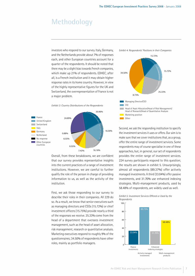
investors who respond to our survey. Italy, Germany, and the Netherlands provide about 7% of responses each, and other European countries account for a quarter of the respondents. It should be noted that there may be a slight bias towards French companies, which make up 21% of respondents. EDHEC, after all, is a French institution and it may obtain higher response rates in its home country. However, in view of the highly representative figures for the UK and Switzerland, the overrepresentation of France is not a major problem.
Exhibit 3: Country Distributions of the Respondents
Overall, from these breakdowns, we are confident that our survey provides representative insights into the current practices of a range of investment institutions. However, we are careful to further qualify the role of the person in charge of providing information to us, as well as the activity of the institution.
First, we ask those responding to our survey to describe their roles in their companies. All 229 do so. As a result, we know that senior executives such as managing directors and CEOs (15.72%) or chief investment officers (15.75%) provide nearly a third of the responses we receive. 25.33% come from the head of a department that oversees investment management, such as the head of asset allocation, risk management, research or quantitative analysis. Marketing executives respond to roughly 9% of the questionnaires; 34.50% of respondents have other roles, mainly as portfolio managers.
Exhibit 4: Respondents’ Positions in their Companies
Managing Director/CEO
CIO
Head of Asset Allocation/Head of Risk Management/Head of Research/Head of Quantitative Analysis
Marketing position
Other
25.33%
15.72%
8.73%
34.50%
15.72%
Second, we ask the responding institution to specify the investment services it uses or offers. Our aim is to make sure that we cover institutions that, as a group, offer the entire range of investment services. Some respondents may of course specialise in one of these approaches, but, in general, our set of respondents provides the entire range of investment services. 224 survey participants respond to this question; the results are shown in exhibit 5. Unsurprisingly, almost all respondents (89.37%) offer actively managed investments. A third (33.04%) offer passive investments, and 31.70% use enhanced indexing strategies. Multi-management products, used by 58.48% of respondents, are widely used as well.
Exhibit 5: Investment Services Offered or Used by the Respondents
0
20
40
60
80
100
58.48%
31.70%
89.73%
33.04%
Passiveinvestments
Enhancedindexing strategies
Actively managedinvestments
Multi-managementproducts
Methodology
France
United Kingdom
Switzerland
Italy
Germany
Netherland
No response
Other European countries
16.16%
16.59%
7.42%
6.55%
6.55%
0.88%
24.89%
20.96%
8 An EDHEC Risk and Asset Management Research Centre Publication
The EDHEC European Investment Practices Survey 2008 - January 2008
Overall, we are confident that the results are representative. Not only do we receive responses from 229 European institutions, but the breakdown of these institutions by assets under management and by country shows that we cover a range of institutions that corresponds broadly to the distribution found in the industry today. In addition, our respondents encompass the entire range of investment services. Finally, survey respondents are usually senior executives or high-level investment specialists.
Choice of TopicsHaving learnt in recent years about the risks of excessive reliance on asset selection models, investors and managers are showing unprecedented interest in asset allocation approaches as sources of performance. This heightened interest in asset allocation has led to innovation on two fronts. First, asset managers and investors are looking at increasingly sophisticated asset allocation methods in order to include more complex risk measures, the problem of parameter estimation, and investment constraints in the asset allocation process. Second, the emergence of alternative asset classes with risk profiles that are very different from those of traditional investments is creating new opportunities for asset allocation in both conceptual and operational terms. This innovation has an impact on the entire investment process, including asset allocation, risk management, and performance measurement. How these innovations have been adopted by industry practices is the focus of the present document. We decide to separate both the questionnaire and the background into four parts, each part addressing an important area of investment practice and the current developments in that area. Below, we address each topic in turn and point out what leads us to devote a large part of our survey to issues related to each topic.
First, we address the use of risk and asset management techniques. The techniques used in the industry are often rooted in academic publications. Often neglected in these publications, however, is the organisation of the investment process.
Recently, the industry has undergone a paradigm change with the adoption of core-satellite management. In this report, we emphasise the usefulness of this approach and establish to what degree it is actually used. In addition, since core-satellite management provides a basic framework, it is interesting to assess which instruments and asset classes are actually considered by practitioners within this framework. When used in practice, academic asset allocation models for portfolio management have come up against numerous obstacles. For example, mean-variance portfolio selection is known to suffer from an extreme sensitivity of weights to the input parameters, as well as from a definition of risk as portfolio volatility, a definition that does not necessarily reflect investor preferences. The solutions that have been proposed to improve portfolio choice models in practice thus revolve around changing the risk measure to more appropriate measures such as Value-at-Risk and around improving the estimation of input parameters. However, if we leave aside anecdotal evidence from industry conferences, it is not clear whether such techniques have been widely adopted. Moreover, the industry today is marked by a proliferation of dynamic trading strategies that are often marketed as structured products. Since the non-linear payoff of the structured product can be replicated by dynamic trading in the underlying asset and cash, a structured product will in effect correspond to a dynamic asset allocation strategy. Therefore, through investing in structured products it may be possible for investors to enjoy the benefits of dynamic asset allocation strategies while using the buy-and-hold investment approach they are comfortable with. However, from a conceptual standpoint, it is a challenge to integrate such strategies into broad asset allocation, since standard asset allocation approaches may not properly account for the non-linear nature of the products. In addition, there are other limits to the adoption of such strategies, including potential regulatory hurdles. One of the results of this survey is to show the dynamic strategies that are currently used and the proportion of institutions that actually use them.
Methodology
9An EDHEC Risk and Asset Management Research Centre Publication
The EDHEC European Investment Practices Survey 2008 - January 2008
We then choose to look at the role of indices and benchmarks in portfolio management. While indices have played a significant role in performance measurement since the dawn of the industry, it should be emphasised that the number of investment products based on indices has multiplied over recent years—these products now include not only traditional index funds, but also exchange-traded funds, options, futures, and other derivatives. In addition to using indices for performance measurement, it is common for investors to use them for investment decision-making, i.e., in the investment processes and portfolio selection models described in the first topic. As part of the decision-making process, they are used either to find an optimal allocation to different indices or even to passively hold a single index that is assumed to be well diversified. However, the standard practice of using a capitalisation-weighting scheme for the construction of indices has been the target of harsh criticism. A number of papers (see, among others, Haugen and Baker 1991, Amenc, Goltz, and Le Sourd 2006, or Hsu 2006) point out that the mechanics of capitalisation weighting lead to trend-following strategies with inefficient risk/return trade-offs. In response to this criticism, equity indices with different weighting schemes now account for a share of index investment products. Of course, these investment products may be completely disregarded when it comes to actual investing, but indices are widely used as benchmark portfolios by investment managers, both for asset allocation and performance measurement purposes. For performance measurement, alternatives to using standard market indices include so-called normal portfolios or customised benchmarks, which are specifically designed to reflect the long-term risk exposure of a specific portfolio or manager, rather than the arbitrary risk exposure of a market index. In view of the many alternatives to standard market indices, it seems appropriate to provide a summary of—as well as some perspective on—recent developments in the area of indices and benchmarking. In addition, a very interesting question is how indexing innovations are perceived by investment practitioners and whether the numerous alternatives to standard
indices, such as customised benchmarks or new forms of indexing, are actually used by a significant proportion of investors and asset managers. And although indices have been in use for the equity class for decades, it is only recently that they have begun emerging for alternative asset classes. We describe the specific challenges to constructing these indices and attempt to establish whether practitioners believe that indexing is plausible when it comes to alternative asset classes. Third, we introduce the problem of asset-liability management (ALM) and describe how to implement a state-of-the-art ALM process. With ALM, it is possible to manage the constraints that stem from future commitments in an institutional investor's balance sheet. It should be noted that ALM is, in a sense, the most general form of asset management. In fact, the asset management techniques covered in the first topic may be perceived as a special case of ALM, where the benchmark return corresponds to the liabilities. Even in the absence of a benchmark, we can replace the latter with the risk-free rate. In practice, however, ALM techniques are largely limited to the investment processes of institutions such as pension funds, a limit that justifies their inclusion as a separate topic. The recent difficulties of liability-constrained investors have drawn attention to their investment practices. A so-called “perfect storm” of adverse market conditions at the turn of the millennium devastated many corporate defined benefit pension plans. Negative equity market returns eroded plan assets at the same time as declining interest rates increased the marked-to-market value of benefit obligations and contributions. In extreme cases, corporate pension plans were left with funding gaps as large as or larger than the market capitalisation of the plan sponsor. That institutional investors in general and pension funds in particular were so dramatically affected by the market downturns emphasises the weakness of investment practices. In particular, it has been argued that the asset allocation strategies implemented in practice, which used to be heavily skewed towards equities without any protection from their downside risk, were not consistent with sound
Methodology
10 An EDHEC Risk and Asset Management Research Centre Publication
The EDHEC European Investment Practices Survey 2008 - January 2008
liability risk management. In this context, a renewed interest in asset-liability management techniques has surfaced in institutional money management. New approaches referred to as liability-driven investment (LDI) solutions have appeared in the wake of recent changes in accounting standards and regulations that have led to an increased focus on liability risk management. As it happens, proposals for techniques to ensure the soundness of liability risk management are not in short supply. From an investor’s perspective, it is important to grasp the meaning of these techniques, to understand the structure of the offers, and to distinguish between real innovation and pure marketing. In the background, we provide an overview of current offers, as well as a theory of ALM. In the results, we compare the theory with current industry practices.
Our fourth topic is performance measurement. When it comes to the investment process, performance measurement is, after the phases completed with some of the techniques described above, the logical finale. Portfolio (or fund) performance evaluation is a key topic, both for managers, who want their skill to be recognised, and for investors, who are seeking the best investment product. The mutual fund market is highly developed and offers a wide range of products. The resulting competition among the different establishments has strengthened the need for clear and accurate portfolio performance analysis. For manager selection, investors want appropriate bases for comparison. They want to know if managers have reached their objectives—that is, if their return is high enough for the risks they have taken, how they compare to their peers, and, finally, whether the portfolio management results are to be put down to luck or to managerial skill that can continue to deliver these results. The portfolio return alone does not provide answers to all of these questions. So, as suggested by the growing body of academic and professional research into performance measurement, an active search for methods that provide information that meets investor expectations is underway. Besides models from portfolio theory, research in the area
of performance measurement has also dealt with real market conditions and developed techniques for cases where the restrictive assumptions of portfolio theory are not observed. At the same time, the choice of a performance measurement technique must reconcile ease of implementation and accuracy and comprehensibility of information. In the sections of this survey devoted to portfolio performance measurement, we provide background information on a range of performance measures and their underlying principles, as well as insights into currently used measures and procedures.
It should be noted that any organisation of the investment process is, to a certain extent, arbitrary. Different institutions may organise their investment processes in completely different ways. Our aim with this questionnaire is to facilitate responses by going from more general to more specific topics. In addition, we address the unifying themes of investment management rather than divide the survey into segments specific to each asset class or to each category of client. In fact, we believe that the common challenges underlying much of the investment process justify this choice. The remainder of the document will first review the investment literature on the four topics introduced in the background and then proceed to the original results of this survey, which reveals current perceptions and practices in the areas of risk and asset management, benchmarking and indices, asset liability management, and performance measurement.
Methodology

Executive Summary
11An EDHEC Risk and Asset Management Research Centre Publication
12 An EDHEC Risk and Asset Management Research Centre Publication
The EDHEC European Investment Practices Survey 2008 - January 2008
This survey assesses the current investment practices of asset management firms, institutional investors, and private wealth managers. Its aim is to give an account of the current practices in the industry and to contrast these practices with the recent state of the art in the investment literature. The survey results are based on a questionnaire that elicited more than two hundred responses from throughout Europe.
We address topics from four central areas of investment management practice: risk and asset allocation, indices and benchmarks, asset-liability management, and performance measurement. The questionnaire is fairly general and focuses on broad aspects and on broad classifications of approaches rather than on technical details. Our analysis of the responses shows that in practice there is a considerable diversity of methods and tools. Overall, however, the results provide evidence that many institutions, rather than fully exploiting the improved techniques that research has made readily available to them, currently settle for the most straightforward.
Risk and Asset Management TechniquesWe turn first to the central tasks of the portfolio management process. In this section, we cover the organisation of portfolio management and the techniques for portfolio optimisation.
Though the techniques used in portfolio optimisation are important for the resulting performance, the organisation of the portfolio management process itself must not be neglected. The core-satellite approach has recently been touted as a superior approach to portfolio management organisation, allowing as it does a clear separation of overperformance of the benchmark and choice of the benchmark management, along with considerable cost savings. The core-satellite approach is now widely used, with more than 50% of those responding to the questionnaire reporting that they use the approach or plan to do so
within the next 12 months. The results show, however, that a number of inconsistencies remain; it is not clear that this new approach is being used to its full potential. Among the inconsistencies are those revealed by the findings on the use of different management approaches within core-satellite portfolios. For example, traditional active management mandates are included in core portfolios, while alternative investments are mainly restricted to the satellite portfolio rather than used as diversifiers in the core. Moreover, it appears that the tracking error management methods that most clearly respect the separation of overperformance of the benchmark and choice of the benchmark have not been widely adopted: portable alpha methods are used by only about 20% of respondents and the completeness portfolio approach by less than 10%.
The results also show that, in addition to the traditional definition of risk as portfolio volatility, portfolio optimisation involves a variety of definitions of risk. In particular, extreme risk measures are now used by a majority of industry participants. However, it turns out that the most popular method used to calculate measures such as VaR or CVaR (chosen by more than 40% of those responding to our questionnaire) is to rely on the assumption of normal distribution, thus ignoring the fact that returns data are typically subject to non-trivial skewness and kurtosis. Only 17% make allowances for higher order moments through approximations such as that of Cornish-Fisher (1937), despite the ease of implementation of these approaches. Thus, more often than not, the so-called extreme risk measures are actually ill-defined.
Our survey also shows that advanced techniques of input estimation and optimisation are not widely used. In fact the predominant approach to covariance estimation remains to use the sample estimator (used by about two-thirds of respondents). This approach leads to maximum sample risk, which could be mitigated by
Executive Summary
13An EDHEC Risk and Asset Management Research Centre Publication
The EDHEC European Investment Practices Survey 2008 - January 2008
techniques that impose some structure on the covariance matrix. Likewise, advances such as the Black-Littermann approach or portfolio resampling, advances that allow the integration of estimation risk, are used by only a minority of survey respondents (less than 20%). More ad hoc ways of avoiding estimation risk, such as imposing constraints on portfolio weights, are preferred.
Overall, although portfolio optimisation is at the heart of investment management, our survey makes it clear that only the most straightforward approaches are widely used and that more recent advances are largely ignored. On the other hand, the organisation of investment management has undergone profound change. The core-satellite approach is now emerging as the leading paradigm among European institutions.
Indices and BenchmarksThe second part of the survey raises a number of questions with respect to the use of indices and benchmarks. One of its aims is to determine the types of indices that are actually used and the criteria by which practitioners judge these indices. Since the indexing industry has seen numerous innovations in recent years, we also attempt to elucidate industry views of these innovations. Therefore, a large part of this topic deals with new indices, those for alternative asset classes as well as new forms of indexing that have recently been introduced in the equity arena.
Analysis of the responses makes it clear that traditional value-weighted indices maintain a very dominant position in spite of the substantial attention accorded new forms of indexing. On average, for example, more than three-quarters of assets under management are indexed to value-weighted indices. Characteristics-based and equal-weighted indices emerge as the most popular alternatives to value-weighted indices, though neither is used by much more than 20% of respondents. It should also be noted that respondents attribute relatively low importance
to the risk and return qualities of standard stock market indices, emphasising instead brand reputation and transparency. On the other hand, respondents are considerably more critical of the newly emerging hedge fund indices. Overall, these results highlight both the major role of indices in the industry and the willingness of respondents to accept indices on the strength of the history and reputation of the provider. With respect to the emergence of alternative indexing forms, it can be stated that there is no clear consensus as to which new form of indexing is preferred. In addition, from the responses we have obtained, we may wonder whether the growth of new forms of indices stems from the problems with value-weighting or simply from a search for return enhancement on the basis of the recent outperformance of these indices.
Asset-Liability ManagementAsset-liability management (ALM) is an investment process that explicitly takes into account the investor’s liability constraints and attempts to manage risk with respect to these constraints. In this section of the survey, we establish how widely the ALM approach is used and what particular techniques predominate.
Overall, the results indicate that ALM techniques are not as widely used in current practice as one might imagine. In particular, it is certainly rather surprising that, in their investment processes, nearly 40% of institutional investors fail to take into account shortfalls with respect to liabilities. Our results suggest that asset-based benchmarks such as the well-known stock market indices are of more concern in current practice than are liability-based benchmarks. It appears to us that more focus is needed on liability relative risk assessment and decision-making.
In addition, those who do consider ALM tend to use relatively straightforward approaches, such as cash-flow matching or LDI products based on immunisation techniques. Surplus optimisation
Executive Summary
14 An EDHEC Risk and Asset Management Research Centre Publication
The EDHEC European Investment Practices Survey 2008 - January 2008
techniques and non-linear risk profiling are used by only a small minority of respondents. Considering that these techniques correspond to well-known management principles in asset management (surplus optimisation corresponds to optimal diversification and non-linear risk profiling to dynamic risk management), this finding is surprising. Cash-flow matching and immunisation, on the other hand, can be seen as investments in the risk-free asset. Low expected returns, of course, are the downside. It is surprising to us that more advanced techniques of managing the risk/return trade-off are not more widely used, given that they are the core business tools of the profession. It should also be noted that this result stands in stark contrast to current practices in a pure asset management framework, in which the vast majority of respondents use some form of portfolio risk optimisation, as shown in the first section.
A further notable result is that measures of extreme risk are not widely used in an ALM context, while in pure asset management, most respondents do use such measures. In fact, only 25.57% of respondents do not account for extreme risk in the general question on portfolio optimisation. Finally, a noteworthy phenomenon is the extensive use of alternatives such as hedge funds and commodities to generate outperformance in the ALM framework.
Performance MeasurementWhile the above sections focus on constructing and implementing portfolios, an important final step—once the benchmark has been defined, the portfolio optimised, and risk controlled—is to assess the outcome of the investment process. This ex-post performance analysis is the topic of the final section of the survey.
It is striking that the performance measures currently used seem to centre on a limited number of standard indicators, such as the Sharpe ratio and the information ratio of a portfolio, used by 80% and 70% of respondents respectively.
Performance measures integrating the notion of downside risk are much less likely to be used. In addition, it turns out that downside risk measures are less widely used in performance measurement than they are in portfolio optimisation, a possibly surprising result, because in portfolio optimisation a single risk objective is often required, whereas in performance measurement, it may be useful to employ a wide range of measures. For this reason, there does not seem to be a good reason not to complement the standard Sharpe ratio with additional performance measures. Furthermore, the results show a frequent use of average returns in excess of the risk-free rate or of the average excess return with respect to a broad market index. In fact, these measures completely ignore the risk exposures of the portfolios under analysis.
Alpha analysis relies heavily on measuring absolute performance in a peer group. This is the predominant measure of alpha, used by nearly two-thirds of respondents, despite the fact that peer groups provide a very coarse adjustment for risk, leading to performance differences within the peer group that can be put down to investment style rather than to managerial skill. Style analysis, which allows precise adjustments with respect to style exposure, proves considerably less popular but is nonetheless used by a significant minority of slightly less than 40% of respondents. As it happens, the use of style analysis to construct a customised benchmark is the least popular choice among possible benchmarks. Only 40% of respondents construct customised benchmarks, while almost 50% choose specific (sector- or style-) indices, and almost 80% use broad market indices. From these results, it can be seen that popularity is inversely proportional to precision. In other words, the benchmarks that provide the crudest risk assessment are the most popular, while those that provide the most detailed risk assessment are the least popular. It should be noted as well that customised benchmarks allow more precise alpha measurement and that the process of customising a benchmark leads to a useful examination of the portfolio risk factors,
Executive Summary

15An EDHEC Risk and Asset Management Research Centre Publication
The EDHEC European Investment Practices Survey 2008 - January 2008
an examination otherwise inexistent (when broad stock market indices are used) or undertaken in a much cruder fashion (when a single sector or style index is used).
Overall, industry practitioners rely largely on simple, well known performance measures to evaluate performance. However, reliance on these measures clearly comes at the cost of precise information on the risks and hence on precise performance measurement and attribution. If the industry wants to make sophisticated risk analysis an integral part not only of portfolio optimisation but also of portfolio evaluation, it will likely need to increase its awareness of modern performance measurement techniques.
Executive Summary

16 An EDHEC Risk and Asset Management Research Centre Publication
The EDHEC European Investment Practices Survey 2008 - January 2008

Background
17An EDHEC Risk and Asset Management Research Centre Publication

18 An EDHEC Risk and Asset Management Research Centre Publication
The EDHEC European Investment Practices Survey 2008 - January 2008
I. Risk and Asset AllocationWe concentrate first on the most basic issues in the investment process—its organisation and the principal techniques for choosing a portfolio of assets and controlling the risk of a portfolio. We present the core-satellite approach and its basic advantages; we emphasise that this organisational framework provides a natural way of managing risk. In addition, this section provides an overview of portfolio selection techniques and has several boxes describing some recent innovations. Finally, to show how investors may benefit from improved risk control through a disciplined dynamic portfolio process, we describe an extension of the static core-satellite approach to a dynamic context. This section thus provides a background not only to the results for risk and asset allocation, but also to subsequent topics, which address more specific aspects of investment techniques and practices.
1.1. Organisation of Portfolio Management 1.1.1. Introduction to the core-satellite portfolio management approachFor most active managers, exposure to a benchmark is still predominantly passive. Instead of paying high fees on the passively managed part of their portfolio, the core-satellite approach suggests passively investing in a low-fee index fund (or an enhanced index product) as a core portfolio and in a variety of active satellite managers with higher tracking error. In its purest form, this approach leads to an investment in market-neutral managers who provide only portable alpha benefits without passive exposure to the index, so that they compensate active managers only for their abnormal returns, not for their passive exposure to rewarded sources of risk.
Driven by the desire to improve investment efficiency, a growing number of institutional investors have, over the past several years, moved to this core-satellite approach to portfolio management. The move towards core-satellite management has brought with it some key changes in the asset management industry, among
them increased demand for high alpha products such as hedge funds, which pursue absolute performance strategies in the absence of tight tracking error constraints.
For risk management, the separation of portfolio management into a core and a satellite allows the manager to define the absolute risk level through the core portfolio and to control the tracking error of the overall portfolio in a straightforward manner through allocation to the satellite. The core portfolio allows a choice of long-term exposure to different asset classes or subcategories and thus defines the absolute risk level. By taking on a certain level of relative risk, the satellite portfolio allows access to out-performance with respect to the core portfolio. This relative risk (tracking error) may be managed statically or dynamically through allocation to the satellite. In the following section, we describe in greater detail the core-satellite portfolio construction methodology, which has lately become the standard for the design of the performance-seeking portfolio.
1.1.2. Benefits of the core-satellite approachA core-satellite portfolio approach can be used as an effective strategy for institutions that want to diversify their portfolios without giving up the potential for higher returns generated by selected active management strategies.
Exhibit 1.1 shows how this approach can be used to set targets for and manage allocations to the core and to the satellite.
Exhibit 1.1: Benefits of the core-satellite approach
Core Satellite Global
Weight 75% 25% 100%
Tracking Error 0% 20% 5%
Illustration of how the core-satellite approach provides benefits to asset managers
Assume that an investor has a relative risk tracking error budget equal to 5%. The first solution is to allocate 100% of the portfolio to an active manager who will commit to this budget. The
Background

19An EDHEC Risk and Asset Management Research Centre Publication
The EDHEC European Investment Practices Survey 2008 - January 2008
second solution consists of allocating 75% of the portfolio to a purely passive product—an exchange traded fund (ETF), for example—or preferably to a strategy that is based on an efficient benchmark, and 25% of the portfolio to a 20% tracking error manager. This solution, consistent with a core-satellite approach to active asset management, offers two benefits.
First, allowing the active manager to deviate significantly from the benchmark leads to a better use of the manager’s skills. If the manager has reliable views on market trends and directions, a 5% tracking error constraint leaves him with too little room for active decisions consistent with these views. Beating the market is notoriously tough. Even harder is to beat it with one hand tied behind your back.
The second benefit is to allow a clear distinction between the value added by the design of the strategic asset allocation represented by the benchmark (core portfolio) and the out-performance generated by active portfolio management.
Indeed, the primary and arguably more important source of added-value is the optimal allocation decision that leads to the design of an efficient core portfolio (see below for state-of-the-art techniques involved in the design of core portfolios). This source of added-value should be rewarded, given that the design of the core portfolio can be a decision from the investor’s part (with the possible help of consultants) or a task delegated to the asset manager. The second source of added-value is the abnormal performance that is generated by active managers, which also deserves a separate reward. Similarly, the manager selection decision can be made by the investor (again with the possible help of consultants) or delegated to a multi-manager.
1.1.3. The arithmetic of core-satellite investingWe consider first a core-satellite approach with a single satellite. We show how to derive the
optimal proportion to invest in the satellite portfolio by setting the problem in a simple mean-variance analysis. We also demonstrate that, if the core portfolio perfectly replicates the benchmark, the information ratio of the overall portfolio is independent of the proportions of wealth in the core and the satellite and equal to the information ratio of the satellite portfolio.
We first consider a core-satellite approach with a single satellite portfolio. The mathematics are then straightforward. The overall portfolio corresponds to:
P = wS + 1-w( )C
where w is the fraction invested in the satellite (S), and 1-w is the fraction invested in the core (C). We now calculate the tracking error with respect to a benchmark B. We obtain:
P - B = wS + 1-w( )C - B = w S - B( ) + 1-w( ) C - B( )
If we now assume for the sake of simplicity that the core portfolio is perfectly replicating the benchmark, we get C=B, then we have:
P - B = w S - B( )As a result, we obtain:
TE P( ) = var P - B( ) = w var S - B( ) = wTE S( )
Consider the following example. We assume an investor has a target level of risk relative to a given benchmark, such as a 2.5% tracking error budget. Two options are possible. Either the investor hires one manager with a tracking error equal to 2.5% for the entire portfolio, or the investor forms a passive core portfolio and leaves 20% in an aggressively managed satellite with a
12.5% =
TE P( )w
=2.5%20%
tracking error.
The next step consists of deriving the optimal proportion w* to invest in either the satellite or the core portfolio. We solve the problem in the context of a simple mean-variance analysis.
Background

20 An EDHEC Risk and Asset Management Research Centre Publication
The EDHEC European Investment Practices Survey 2008 - January 2008
The optimisation program reads:
where IR(P) is the information ratio of the portfolio P with respect to the benchmark:
IR P( ) =
E(P - B)σ(P - B)
=E(P - B)TE P( )
(see, for, example Grinold and Kahn 2000).
When the core portfolio perfectly replicates the benchmark, the information ratio of the overall portfolio IR(P) is actually independent of the proportions of wealth invested in the core and the satellite and equal to the information ratio of the satellite portfolio IR(S) (as long as the proportion w is strictly positive). This can easily be seen from:
We may rewrite the optimisation program as:
U w( ) = IR ×w ×TE( S) - λw 2TE 2( S )
and the first-order condition reads:
∂U∂w
w*( ) = 0 ⇒w* =IR
2λTE S( ) For example, let us assume that the tracking error of the active fund is 5%, that the information ratio (IR) is 0.5, and that the coefficient of risk-aversion with respect to relative risk is λ = 0.2. Then, the optimal proportion invested in the active portfolio is:
w* =IR
2λTE S( )=
.52 × .2 ×5%
= 25%
The resulting tracking error is
TE P( ) = 25% ×5% =1.25%
Extending the analysis to the case of a satellite
S = wi Si
i =1
n
∑ invested in a number n of active
portfolio managers iS according to the proportions iw is straightforward. The excess return on the satellite portfolio is then:
S - B = wi Si - B( )
i =1
n
∑
and the tracking error of the satellite portfolio reads:
TE S( ) = wiwj σij
i , j =1
N
∑ - 2 wi σiB + σB2
i =1
N
∑⎛
⎝⎜⎞
⎠⎟
12
where ijσ is the covariance between portfolio managers iS and jS , and Bσ is the volatility of the benchmark.
It is then possible to find the optimal fraction invested in each active manager within the satellite portfolio so as to achieve the highest possible information ratio. Scherer (2002), among others, has shown that the optimal condition is that the ratio of return to risk contribution be the same for all managers:
wk αk
wk2σαk
2 + wkwj σkjj
∑⎛
⎝⎜⎞
⎠⎟
TE( S)
=wl αl
wl2σα l
2 + wlwj σkjj
∑⎛
⎝⎜⎞
⎠⎟
TE( S )
1.2. Diversification: Optimal Beta ManagementStrategic allocation is the first step in the investment management process. This step involves choosing from among the different asset classes or styles that, in accordance with the investor’s objectives, will make up the portfolio. Thus, strategic allocation defines the core. Strategic allocation may be done for the overall portfolio of assets or for a given asset class. In the latter case, the strategic allocation will determine the exposure to different subcategories (styles or sectors) of a given asset class (stocks, bonds, or alternative assets). It is also possible to
Background
U = E(P - B) - λσ 2(P - B) = IR P( ) ×TE P( ) - λTE 2 P( )
IR P( ) =
E(wS + 1-w( )C - B)σ(wS + 1-w( )C - B)
=wE( S - B)wTE S( )
= IR S( )
21An EDHEC Risk and Asset Management Research Centre Publication
The EDHEC European Investment Practices Survey 2008 - January 2008
construct an optimal allocation for a given asset class directly from the individual assets. For each level of granularity (that is, the overall portfolio or the portion for a given asset class), it is necessary to define a core portfolio that willallow control and management of the strategic allocation. Today, asset allocation is playing a greater role in the investment management process. This interest in asset allocation can be explained by the results established by various empirical studies, which suggest that this step can contribute significantly to the result of the portfolio. Brinson, Hood, and Beebower (1986) and Brinson, Singer, and Beebower (1991) have shown, for example, that a considerable share (90%) of a portfolio’s performance can be attributed to the initial allocation decision.
Contrary to a common misperception, managing the core portfolio does not necessarily imply passive investment in a commercial index. It consists instead of using state-of-the-art asset allocation techniques to design an optimal benchmark based on investor preferences and constraints, liability constraints in particular.
Strategic allocation was formalised by the seminal work of Markowitz (1952), who was the first to quantify the link between the risk and return of a portfolio, and thereby introduced modern portfolio theory. Markowitz developed a theory of portfolio choice in an uncertain future based on a quantification of the difference between the risk of a portfolio’s assets taken individually and the global portfolio risk. His theory relates to maximising the utility of final wealth for a risk-averse investor, who measures risk through the variability of asset returns (volatility). Optimal portfolios, from a rational investor’s point of view, are defined as the portfolios with the lowest level of risk for a given return, or equally, as the portfolios with the highest return for a given level of risk. These portfolios are said to be efficient in the mean-variance sense.
Markowitz’s portfolio selection method therefore involves obtaining an optimal portfolio as a function of first order (expected return) and second order (variance and covariance) moment estimations of the returns of the asset classes under consideration. The quality of the estimation of these parameters is all the more decisive in that it has been shown that the portfolio optimisation program is characterised by very significant dependence on the initial conditions: minor discrepancies in the estimation of the parameters lead to very significant changes in the optimal allocation. This problem has been shown to be particularly acute in the case of errors in expected return estimation (Chopra and Ziemba 1993). As a result of the lack of robustness in Markowitz efficient frontier analysis, it has been suggested to focus on the only portfolio for which expected return estimates are not needed—the minimum variance portfolio. The key challenge then is to use a robust methodology for an enhanced estimation of the asset returns variance-covariance matrix, a problem that has been extensively studied in the literature. In the following section, we provide an overview of the main findings on how to mitigate the sample risk problem in the estimation of the second-order moments and co-moments of asset return distribution.
1.2.1. Enhanced estimates of covariance matricesSeveral solutions to the problem of asset return covariance matrix estimation have been suggested in the traditional investment literature. The most common estimator of return covariance matrix is the sample covariance matrix of historical returns.
S =
1T -1
Ht - H( ) Ht - H( ) '
t =1
T
∑
where T is the sample size, Ht is an Nx1 vector of returns in period t, N is the number of assets in the portfolio, and
H =
1T
Htt =1
T
∑
Background
22 An EDHEC Risk and Asset Management Research Centre Publication
The EDHEC European Investment Practices Survey 2008 - January 2008
is the average of these return vectors. We denote by Sij the (i,j) entry of S.
A problem with this estimator is typically that a covariance matrix may have too many parameters for the available data. If the number of assets in the portfolio is N, there are indeed N(N-1)/2 different covariance terms to be estimated. Because data are scarce, the problem is particularly acute in the context of alternative investment strategies, even when a limited set of funds or indices is considered; more often than not, after all, returns on alternative investments are available only infrequently.
One possible cure for the curse of dimensionality in covariance matrix estimation is to structure the covariance matrix in such a way as to reduce the number of parameters to be estimated. Of course, this cure invites two very important questions: how much structure should we impose? (the fewer the factors, the stronger the structure) and what factors should we use? There is a standard trade-off between model risk and estimation risk. The following options are available:
• Impose no structure. This choice involves low specification error and high sampling error, and leads to the use of the sample covariance matrix.1
• Impose some structure. This choice involves high specification error and low sampling error. Several models, including the single factor forecast (Sharpe 1963) and the multi-factor forecast (e.g., Chan, Karceski, and Lakonishok 1999), fall within this category. Another way to impose structure on the covariance matrix is to use the constant correlation model (Elton and Gruber 1973). This model can also be thought of as a James-Stein estimator that shrinks each pairwise correlation to the global mean correlation.
• Impose optimal structure. This choice involves medium specification error and medium sampling error. The optimal trade-off between specification
error and sampling error leads to optimal shrinkage towards the grand mean (Jorion 1985, 1986), to optimal shrinkage towards the single-factor model (Ledoit 1999), or to the introduction of portfolio constraints (Jagannathan and Ma 2003).
Another alternative is to consider an implicit factor model in an attempt to mitigate model risk and impose endogenous structure. The advantage of this alternative is that it involves low specification error (because of its “let the data talk” approach) and low sampling error (because some structure is imposed). Implicit multi-factor forecasts of asset return covariance matrix can be further improved by noise-dressing techniques and optimal selection of the relevant number of factors (see below). More specifically, we use principal component analysis (PCA) to extract a set of implicit factors. The PCA of a time-series involves studying the correlation matrix of successive shocks. Its purpose is to explain the behaviour of observed variables using a smaller set of unobserved implied variables. Since principal components are chosen solely for their ability to explain risk; a given number of implicit factors always captures a larger part of asset return variance-covariance than does the same number of explicit factors. One drawback is that implicit factors do not have a direct economic interpretation (except for the first factor, which is typically highly correlated with the market index). Principal component analysis has been used in the empirical asset pricing literature (Litterman and Scheinkman 1991, Connor and Korajczyk 1993, or Fedrigo, Marsh, and Pfleiderer 1996, among many others). From a mathematical standpoint, PCA involves transforming a set of N correlated variables into a set of orthogonal variables, or implicit factors, which reproduces the original information present in the correlation structure. Each implicit factor is defined as a linear combination of original variables. Define H as the following matrix:
Background
1 - One possible generalisation/improvement to this sample covariance matrix estimation is to assign declining weights to observations as they go further back in time (Litterman and Winkelmann 1998).
23An EDHEC Risk and Asset Management Research Centre Publication
The EDHEC European Investment Practices Survey 2008 - January 2008
H = hit( )1≤t ≤T
1≤i ≤N
We have N variables hi , i=1,...,N, i.e., returns for N different assets, and T observations of these variables.2 PCA enables us to decompose htk as follows:3
htk = λi
i =1
N
∑ UikVti : = siki =1
N
∑ Vti
where U is the matrix of the N eigenvectors of H’HV is the matrix of the N eigenvectors of HH’
Note that these N eigenvectors are orthonormal. λi is the eigenvalue (ordered by degree of magnitude) corresponding to the eigenvector Ui. Note that the N factors Vi are a set of orthogonal variables. The main challenge is to describe each variable as a linear function of a reduced number of factors. To that end, one needs to select a number of factors K such that the first K factors capture a large fraction of asset return variance, while the remainder can be regarded as statistical noise:
htk = λi
i =1
K
∑ UikVti + εtk : = siki =1
K
∑ Vti + εtk
where some structure is imposed by assuming that the residuals εtk are uncorrelated. The percentage of variance explained by the first K factors is given by:
λii =1
K
∑
λii =1
N
∑
A sophisticated test by Connor and Korajczyk (1993) finds between 4 and 7 factors for the NYSE and AMEX over the period from 1967 to 1991, which is roughly consistent with the findings of Roll and Ross (1980). Ledoit (1999) uses a 5-factor model. We can select the relevant number of factors by applying some explicit results from the theory of random matrices (Marchenko and Pastur
1967).4 The idea is to compare the properties of an empirical covariance matrix (or, likewise, of a correlation matrix, since asset returns have been normalised to have zero mean and unit variance) to a null hypothesis purely random matrix such as one could obtain from a finite time-series of strictly independent assets. It has been shown (see Johnstone 2001 and Laloux et al. 1999 for an application to finance) that the asymptotic density of eigenvalues λ of the correlation matrix of strictly independent assets reads:
f λ( ) =T
2πN
λ - λmax( ) λ - λmin( )λ
λmax =1+NT
+ 2NT
λmin =1+NT
- 2NT
Theoretically speaking, this result can be exploited to provide formal testing of the assumption that a given factor represents information and not noise. However, the result is an asymptotic result that cannot be taken at face value for a finite sample size. One of the most important features here is that the lower bound of the spectrum λmin is strictly positive (except for T=N), and therefore, there are no eigenvalues between 0 and λmin. We use a conservative interpretation of this result to design a systematic decision rule and decide to regard as statistical noise all factors associated with an eigenvalue lower than λmax. In other words, we take K such that λK > λmax and λK+1 < λmax, where λ1 is the greatest eigenvalue.5
A problem of a different nature comes from the non-stationarity of the data. Numerous empirical studies have pointed out, for example, that the volatilities of asset classes are not constant over time and that an optimisation where the risk parameters are set equal to their past values would not, as a result of their non-stability, be very robust. The dynamic character of the parameters
Background
2 - The asset returns have first been normalised to have zero mean and unit variance.3 - For an explanation of this decomposition in a financial context, see Barber and Copper (1996).4 - Another decision rule would be: keep enough factors to explain x% of the covaria-tion in the portfolio.5 - If no factor is such that the associated eigenvalue is grea-ter than λmax, we take K=1, i.e., we retain the first component as the only factor.
24 An EDHEC Risk and Asset Management Research Centre Publication
The EDHEC European Investment Practices Survey 2008 - January 2008
renders the task of estimation more arduous, a challenge that can be addressed by the use of suitably designed statistical models such as Garch models. Good modelling brings robustness back to portfolio optimisation over a long period by relying on the stability of the models that define the variation in the risk parameters (variance-covariance) and no longer on the stability of the risk parameters themselves.
While it appears that there are a large number of techniques that can be used to allow better estimation of the variance-covariance matrix of asset returns, a major challenge remains: that of estimating the mean returns. It is for this reason that it has been suggested to focus on minimum risk portfolios whose derivation does not depend on any estimate of expected returns.6
1.2.2. Accounting for extreme risk measuresOne important limitation in Markowitz analysis is that volatility is used as the definition of risk. Going back to the basics of utility-maximisation, we note that the mean-variance approach, provided non-normal asset returns, is in fact only a second-order approximation of a general utility function.
To take higher moments into account, we consider any arbitrary utility function. The investor is assumed to be maximising the utility emanating from wealth invested in a portfolio with a return denoted by R. The fourth-order Taylor expansion gives us:
where U(k) denotes the kth derivative of the function U. Taking the expectation on both sides yields:
with the centralised moments:
μ 2( ) R( ) = Ε R - Ε R( )( ) 2⎡⎣
⎤⎦
μ 3( ) R( ) = Ε R - Ε R( )( ) 3⎡⎣
⎤⎦
μ 4( ) R( ) = Ε R - Ε R( )( ) 4⎡⎣
⎤⎦
Thus, we can approximate any utility function of a portfolio return as a function of expected portfolio return and standard deviation, but also as a function of third and fourth moments of the portfolio return distribution. The mean-variance corresponds to a second-order approximation that is, of course, less exact.
One could argue that, in the real world, investors are not only interested in maximising expected return and minimising volatility, but also in limiting the loss with a given probability (1-α). It is for this reason that our objective shall focus on a measure like Value-at-Risk at (1-α)%, which is defined as the negative value of the α-quantile of the underlying return distribution. Assuming a normal distribution, this measure is given simply by:
VaR(1-α ) = -( μ + zα σ )
with zα the α-quantile of the standard normal distribution.
Because asset returns are generally not normally distributed, we should incorporate higher moments in the Value-at-Risk measure. This can be done through a method called a Cornish-Fisher expansion (see Jaschke 2002 for a detailed description), which approximates distribution percentiles in the presence of non-Gaussian higher moments. The Cornish-Fisher expansion is derived from the general Gram-Charlier expansion, using
Background
6 - An interesting attempt to improve portfolio allocation techniques in the presence of uncertain expected return parameter estimates can be found in Black and Litterman (1992).
U( R) =
U ( k )( E( R))k!
( R - E( R)) k⎡
⎣⎢
⎤
⎦⎥
k =0
4
∑ + ο R - E( R)( ) 4⎡⎣
⎤⎦
E[U( R)] ≈U( E( R)) +
U ( 2 )( E( R))2
μ 2( ) R( ) +U ( 3 )( E( R))
6μ 3( ) R( ) +
U ( 4 )( E( R))24
μ 4( ) R( )
E[U( R)] ≈U( E( R)) +
U ( 2 )( E( R))2
μ 2( ) R( ) +U ( 3 )( E( R))
6μ 3( ) R( ) +
U ( 4 )( E( R))24
μ 4( ) R( )
25An EDHEC Risk and Asset Management Research Centre Publication
The EDHEC European Investment Practices Survey 2008 - January 2008
the standard normal distribution as the reference function. For a four-moment approximation of α-percentiles the following formula is given:
where S denotes the sample skewness, K the sample’s excess kurtosis and αz the α -percentile of the standard normal distribution. αz~ denotes the modified α -percentile. This approximation is built on the hypothesis that the underlying distribution is close to a normal distribution. We obtain the modified Value-at-Risk measure with confidence (1-α ):
VaRmod(1-α ) = - (μ + αz~ σ)
where σ denotes estimated values for the standard deviation and μ the mean.
Another relevant measure of extreme risk is the Conditional Value-at-Risk (CVaR), defined as the expected loss beyond the VaR, which focuses on the left tail of the returns distribution beyond a threshold, as opposed to a mere certain quantile as VaR does. Interestingly, CVaR would also be a preferred risk objective from an optimisation perspective. VaR is difficult to optimise when it is calculated over scenarios because it leads to non-convex optimisation problems; there are multiple extrema and the local optimisation algorithms are unsuccessful, whereas the global algorithms are inefficient. On the other hand, CVaR can be optimised through stochastic linear programs (Rockafellar and Uryasev 2000).7
In addition, VaR can in fact be used as a portfolio risk management tool. To achieve this objective, it must be possible to define the composition of a portfolio’s VaR and to analyse the impact of a new transaction on the total VaR of the portfolio. This is the objective of incremental VaR calculations. The goal of the incremental VaR is precisely to define the contribution of each asset to the total VaR of the portfolio. The total VaR of the portfolio is not equal to the sum of the VaRs of the assets that make up the portfolio, because there are correlations between the assets. The incremental VaR, for its part, is defined in such a way that the sum of the incremental VaRs is equal to the total VaR of the portfolio. It is obtained from the delta VaR, which is the vector of the VaR’s sensitivity to each asset. It is made up of partial derivatives of the portfolio’s VaR with respect to each asset. The incremental VaR of asset i is then calculated by multiplying the ith component of the portfolio's VaR delta by the quantity of asset i held. If we denote the proportion of asset i held in the portfolio as ix , the incremental VaR for asset i in portfolio P, denoted by )(PIVaR i , is given by:
IVaRi (P ) = xi
∂VaR(P )∂xi
If the incremental VaR of an asset is positive, it contributes to an increase in the total VaR of the portfolio. On the other hand, if the incremental VaR of the asset is negative, introducing it into the portfolio will decrease the total VaR.
Background
7 - At first, CVaR calculation seems to be complex, since it depends on the VaR itself, but little optimisation tricks can make it possible to calculate CVaR in an optimisation problem without having to know the VaR value. And, interestingly, optimisation of CVaR will help calculate VaR for that same level, as further explained in Rockafellar and Uryasev (2000).
%zα = zα +
16
( zα
2 -1)S +1
24( zα
3 - 3zα )K -1
36( 2zα
3 -5zα )S 2αz~
Improving Estimation of Higher Order Moments and Co-moments
It is clear that extending the risk space from one dimension (volatility) to three dimensions (volatility, 3rd and 4th central moments) increases exponentially the number of parameters to estimate. This ex-tension calls for robust estimation techniques such as structural estimators described in section 1.2.2 for the case of the variance-covariance matrix. As Martellini and Ziemann (2007) have shown, the constant correlation approach as well as the single factor approach may be extended to the context of higher order moments.

26 An EDHEC Risk and Asset Management Research Centre Publication
The EDHEC European Investment Practices Survey 2008 - January 2008
Indeed, the single factor model is characterised by the projection of single asset returns (R) on the returns of a broad market index (F):
Rt = c + βFt + εt
On the assumption of uncorrelated residuals the covariance matrix may then be decomposed as:
Σ̂ = ββ' Var( F ) +Ψ̂
where Ψ̂ is supposed to be a diagonal matrix containing the estimated idiosyncratic variances. Consistent with the projection idea, suitable matrix manipulation techniques can be used to extend the model to the context of higher order co-moments. As demonstrated in Martellini and Ziemann (2007), the higher order co-moments of the portfolio can be written as:
μ 2( ) = ω ' M2ω
μ 3( ) = ω ' M3 ( ω ⊗ ω )
μ 4( ) = ω ' M4 ( ω ⊗ ω ⊗ ω )
with
As a result, the authors derive the single factor estimates of the corresponding higher order co-mo-ments as:
μ̂ 2( ) = ( ββ ') μ̂0
2( ) +Ψ̂
μ̂ 3( ) = ( ββ ' ⊗ β ') μ̂0
3( ) + Φ̂
μ̂ 4( ) = ( ββ ' ⊗ β ' ⊗ β ') μ̂0
4( ) + Υ̂
where ( )k
0μ̂ denotes the k-th central moment of the market index returns. The elements in Φ̂ and Υ̂ are obtained in accordance with the assumption of independent regression residuals.
As far as the constant correlation approach is concerned, the Cauchy-Schwartz inequality is used to define higher order correlation constants that are consistent with the Pearson correlation coefficient on the second order level. We recall this fundamental inequality:
E( XY )[ ] 2≤ E( X )E(Y )
If we let X and Y be centralised returns of some assets, this relation implies that the Pearson correla-tion coefficient (r) is bounded by 1:
r 2 =
E( XY )[ ] 2
E( X )E(Y )≤1
Accordingly, we can suitably define X and Y (excess, squared excess, and cubic excess returns of assets) so as to model all possible combinations of higher order co-moments and the corresponding higher order correlation coefficients. As a result, consistent with the formulas obtained in the case of the covariance matrix, higher order co-moments—that is, all elements in M2, M3, and M4—may be com-puted merely based on seven correlation coefficients and centralised univariate moments of the asset returns (Martellini and Ziemann 2007).
Background
M2 = Ε R - Ε R( )( ) R - Ε R( )( )'⎡⎣ ⎤⎦
M3 = Ε R - Ε R( )( ) R - Ε R( )( )' ⊗ R - Ε R( )( )'⎡⎣ ⎤⎦
M4 = Ε R - Ε R( )( ) R - Ε R( )( )' ⊗ R - Ε R( )( )' ⊗ R - Ε R( )( )'⎡⎣ ⎤⎦

27An EDHEC Risk and Asset Management Research Centre Publication
The EDHEC European Investment Practices Survey 2008 - January 2008
Both models considerably reduce the number of unknown parameters. Applying the sample estimators to calibrate a four-moment asset allocation model for portfolios containing 25 assets, for instance, re-quires 80 years of monthly data to ensure that the number of unknown parameters (23,725) does not exceed the number of observations. On the contrary, to fully establish estimates for the second, third, and fourth co-moment matrices (in M2, M3, and M4) for the same portfolio of 25 assets, the constant correlation and the single factor based estimations require only 103 and 107 parameters respectively. This leads to statistically well defined systems.
As shown in Martellini and Ziemann (2007), the gains due to the reduction of estimation risk over-come the losses due to specification error implied by the model restrictions and lead to statistically significant gains in out-of-sample utilities. Moreover, empirical evidence suggests that structural es-timators enhance the stability of portfolios as measured by the turnover rate in a rolling window portfolio construction framework. Consequently, the proposed structural estimators allow investors to take higher order moments into account without excessively increasing the number of parameters to estimate.
Background
8 - More generally, this reverse-engineering mechanism can be applied to infer the expected return estimate that can support any given asset allocation, and not necessarily an asset allocation corresponding to market cap weightings. 9 - Note that λ is the market risk aversion coefficient.
1.2.3. Enhanced estimates of expected returnsTo obtain expected returns as an input to portfolio optimisation, it is often useful to employ a beta pricing model. These models postulate a (usually linear) relation between the expected returns on an asset and the asset’s exposure to a number of risk premia. They may be used to create views on expected returns, given a prediction of risk premia and of risk factor exposures. In this section, we present a formal model that integrates views on expected returns into an asset allocation process. We provide a review of the Black-Litterman model. An extension to a setup where higher moments of return distribution are taken into account is pro-vided in an insert.
Since the seminal work of Markowitz (1952) there has been a strong consensus in portfolio manage-ment on the trade-off between expected return and risk. In the Markowitz world, risk is represen-ted by standard deviation. Given the investor's specific risk aversion, optimal portfolios and the so-called efficient frontier can be derived. Using this mean-variance approach, Sharpe (1964) and Lintner (1965) design an equilibrium model, the capital asset pricing model (CAPM), whose aim is to describe asset returns. Assuming homogenous beliefs, every investor holds the market portfolio derived from this equilibrium model.
Subsequently, Black and Litterman (1990, 1992) propose a formal model based on the desire to combine neutral views consistent with market equilibrium and individual active views. They in-troduce confidence levels on the prior distribu-tion and on individual beliefs and obtain the joint distribution. Through a Bayesian approach, the expected return incorporates market views and individual expectations. The Black-Litterman ap-proach, in its original form, can be summarised as the following multi-step process (Idzorek 2004).
With the risk aversion coefficient (λ), the historical variance covariance matrix (Σ), and the vector of market capitalisation weights (ωM), the vector of implied equilibrium returns in excess of the risk-free rate can be obtained as:8
Π = λΣωM
This approach, of course, is equivalent to using a standard capital asset pricing model. The parame-ter λ can thus be rewritten as:9
λ =
E RM( ) - RF
σM2
⎛
⎝⎜⎞
⎠⎟
where the indices F and M denote the risk-free rate and the market portfolio respectively.

28 An EDHEC Risk and Asset Management Research Centre Publication
The EDHEC European Investment Practices Survey 2008 - January 2008
Individual active views, based on forecasting procedures, for example, are then introduced. These k views can be relative or absolute and are represented in the kx1-vector Q. The kxn-projection matrix P will be used to define these views:
Q = P ⋅RA
A confidence level will be associated with each of the views expressed in Q. Thus, the individual beliefs can be described by a view distribution.10
P ⋅RA ~ N(Q,Ω ).
In the same way, it is possible to define the confidence in the equilibrium model and the derived implied returns. Consequently, we obtain the prior equilibrium distribution:
RN ~ N( Π ,τΣ ).
Ω and τ have to be calibrated. We will come back to this problem in section 4.
In accordance with the Bayesian rule, the two distributions are combined (see Satchell and Scowcroft 2000) to yield the following distribution:
RBL ~ N E( RBL ), τΣ( ) -1
+P' Ω -1P⎡⎣
⎤⎦
-1⎛⎝⎜
⎞⎠⎟
where
This distribution incorporates both the neutral (equilibrium) and the active views. Taking this expected return as an input, the optimal Black-Litterman portfolio weights (ωBL) are then given by:
ωBL = λΣ( ) -1E( RBL )
Background
10 - In all these Bayesian approaches normal distributions are assumed.
E( RBL ) = τΣ( ) -1
+P' Ω -1P⎡⎣
⎤⎦
-1
τΣ( ) -1Π +P' Ω -1Q⎡
⎣⎤⎦
(1)
An Extension to Higher Moments
While the Black-Litterman model is well-suited for portfolio construction in the context of active asset allocation decisions, it suffers from an important limitation: it is based on the Markowitz model, where volatility is used as the definition of risk.
To enable the application of a Black-Litterman model to assets with non-normal distribution, we first suggest extending this model by taking higher moments into account and so turning it into a four-moment portfolio selection model.
Portfolio allocation with higher momentsThe first step is to derive the neutral expected returns that enter the Black-Litterman formula.
MωλΣ=Π , incompatible with the non-normality assumption and the consideration of higher moments, cannot be the appropriate formula.
Going back to the basics of utility-maximisation, we note that the mean-variance approach is, given non-normal asset returns, only a second-order approximation of a general utility function.
To take higher moments into account, we consider any arbitrary utility function. The investor is assumed to be maximising the utility emanating from wealth invested in a portfolio with return denoted by R. The fourth-order Taylor expansion gives us:
U( R) =
U ( k )( E( R))k!
( R - E( R)) k⎡
⎣⎢
⎤
⎦⎥
k =0
4
∑ + ο R - E( R)( ) 4⎡⎣
⎤⎦

29An EDHEC Risk and Asset Management Research Centre Publication
The EDHEC European Investment Practices Survey 2008 - January 2008
Background
where U(k) denotes the kth derivative of the function U. Taking the expectation on both sides yields:
E[U( R)] ≈U( E( R)) +
U ( 2 )( E( R))2
μ 2( ) R( ) +U ( 3 )( E( R))
6μ 3( ) R( ) +
U ( 4 )( E( R))24
μ 4( ) R( )
with the centralised moments:
μ 2( ) R( ) = Ε R - Ε R( )( ) 2⎡⎣
⎤⎦
μ 3( ) R( ) = Ε R - Ε R( )( ) 3⎡⎣
⎤⎦
μ 4( ) R( ) = Ε R - Ε R( )( ) 4⎡⎣
⎤⎦
Thus, we can approximate any utility function of a portfolio return as a function of expected portfolio return and standard deviation, but also as a function of third and fourth moments of the portfolio return distribution. The mean-variance corresponds to a second-order approximation that is, of course, less exact. The new maximisation problem yields:
max
ωΦ μ( RP ),μ 2( ) Rp( ) ,μ 3( ) Rp( ) ,μ 4( ) Rp( )( )
Such that
ωii =1
n
∑ =1-ω0 .
with:
(2)
μ( RP ) = E(ω ' R ) +ω0 R0 = ω ' E( R) +ω0 R0
μ 2( ) Rp( ) = ω ' E R - E( R)( ) R - E( R)( )'⎡⎣ ⎤⎦ω = ω ' Σω
μ 3( ) Rp( ) = ω ' E R - E( R)( ) R - E( R)( )' ⊗ R - E( R)( )'⎡⎣ ⎤⎦ ω ⊗ω( ) = ω ' Ωω
μ 4( ) Rp( ) = ω ' E R - E( R)( ) R - E( R)( )' ⊗ R - E( R)( )' ⊗ R - E( R)( )'⎡⎣ ⎤⎦ ω ⊗ω ⊗ω( ) = ω 'Ψω .
where ⊗ denotes the Kronecker-product, R=(R1,…,Rn)’ the vector of asset returns, ω=(ω1,…,ωn)’ the vector of portfolio proportions invested in these assets, ω0 the position held in the risk-free asset (return R0) and μ=(μ1,…,μn)’ the mean return vector. Ωω is the vector of co-skewnesses for the weighting vector ω and Ψω the vector of co-kurtosises respectively. We take this matrix representation from Jondeau and Rockinger (2004), who use it in a different approach.
Solving the problem as in Hwang and Satchell (1999), for example, we obtain:
μ - R0 = α1 β ( 2 ) +α2 β ( 3 ) +α3 β ( 4 )
(3)with β(i) the vectors of portfolio betas defined as (see Martellini and Ziemann 2005 for an interpretation of these beta coefficients):
β ( 2 ) =
Σω
μ 2( ) Rp( )β ( 3 ) =
Ωω
μ 3( ) Rp( )β ( 4 ) =
Ψω
μ 4( ) Rp( ) (4)
The variables αi can be understood as the risk premia associated with covariance, coskewness and cokurtosis respectively. Hence, we have obtained a four-moment capital asset pricing model similar to that of Hwang and Satchell (1999).

30 An EDHEC Risk and Asset Management Research Centre Publication
The EDHEC European Investment Practices Survey 2008 - January 2008
One possibility to obtain the iα̂ estimates is a simple GLS-regression. However, we are often limited to small samples. In this case, the natural reaction is to introduce a specific model, which comes at the cost of specification risk, of course, to mitigate sample risk. As in Jondeau and Rockinger (2004), we assume a specific representative utility function. For its appealing parameter interpretation, we have chosen the constant absolute risk aversion function )()( WeWU λ--= .
The risk premia (see Hwang and Satchell 1999 or Jondeau and Rockinger 2004) are then:
α1 =
λμ 2( ) Rp( )A
α2 = -λ 2μ 3( ) Rp( )
2Aα3 =
λ 3μ 4( ) Rp( )6A (5)
with A =1+
λ 2
2μ 2( ) Rp( ) -
λ 3
6μ 3( ) Rp( ) +
λ 4
24μ 4 Rp( )
(6)
The risk aversion parameter λ can be calibrated with respect to historical data. Here we use long-term estimates based on the stock return estimates from 1900-2000 for 16 countries by Dimson, Marsh, and Staunton (2002) to obtain λ=2.14, based on a 6.20% risk premium and 17% volatility (Dimson, Marsh, and Staunton, page 311). The various co-moments are estimated over the entire sample period from January 1997 to December 2004.
It is important to note that the vectors of portfolio betas as well as the risk premia (αi) are functions in the weighting vector ω (see equations (2)-(6)). Thus, equation (3) gives us a deterministic relationship between the expected returns (left-hand side) and the weighting vector (right-hand side). Built on the hypothesis of homogeneous expectations, this equation represents a pricing relationship for a distinct market segment and can be used in two different ways:
i) to obtain expected returns11 based on exogenous portfolio weights.ii) to obtain the weighting vector based on exogenous expected returns.
The idea is that equation (3) yields a non-linear equation system with n equations and n unknowns that can be solved using standard numerical methods.
Background
11 - These are obtained endogenously and sometimes called implied equilibrium returns.
1.3. Risk Management in the Core-Satellite Approach1.3.1. Core-satellite and risk budgeting So far, we have assumed that the fund tracking error is known and solving the problem of satellite portfolio allocation has consisted of calculating the weightings to be assigned to each part of the satellite. It is also possible to consider the case of a satellite where allocation to different managers is fixed and where optimisation consists of choosing the level of tracking error to assign to each manager depending on his ability. This approach seeks the optimal allocation to the various managers and
proceeds with a risk allocation rather than with a weight allocation. Weight allocation, currently used in portfolio management, assigns a high weight to the best managers and a low weight to those whose performance is inferior. The risk allocation method, by contrast, assigns the same weight to all the managers but allows the best ones to employ more offensive management with a higher risk level, as measured by the tracking error. Risk allocation makes it possible to find both the optimal portfolio proportion to invest in the satellite and the optimal combination of allocations to satellite funds.

31An EDHEC Risk and Asset Management Research Centre Publication
The EDHEC European Investment Practices Survey 2008 - January 2008
The return of a satellite portfolio is given by:
α = wi φi αi
i
∑
where i
α is the return of the ith manager and
iφ is a scale factor, 0≥iφ .
Setting iiiw φω = , the risk of a satellite
portfolio is given by:
σ(α ) = ( ωi ω j σij )1/ 2
j
∑i
∑
where ijσ denotes the covariance between the alpha generated by the different managers.
Optimising the risk budget and, hence, simultaneously determining the global active allocation and the allocation to managers is done by minimising total portfolio risk subject to an alpha constraint:
Min
σ = ( ωi ω j σij )1/ 2
j
∑i
∑
subject to:
α = ωi αi
i
∑The optimal risk allocation to the active managers and the active share of the portfolio are derived by maximising the alpha of the whole portfolio under a risk constraint. The optimality conditions are given by:
αi =
α
σ⎛⎝⎜
⎞⎠⎟
dσ
dωi
and:
αi
α j
=dσ
dωi
/dσ
dω j
The optimal risk allocation implies that, for each portfolio, the ratio between its marginal contribution to alpha and its marginal contribution to risk is equal to its information ratio.
1.3.2. The completeness portfolio approach and portable alphaThe composition of the satellite, which is the active part of a core-satellite portfolio, should
stem from a focus on selecting the manager(s) with the highest potential for generating alpha. But nothing guarantees that the resulting satellite portfolio will have the same factor exposure as that of the core, which, given investor preferences and constraints, was designed to be optimal. Furthermore, chances are that a naïve selection of active managers will lead to an undoing of the otherwise carefully designed factor exposure of the core portfolio. Two possible approaches can be taken to align the betas of the satellite to the betas of the core. The first consists of optimising the manager’s portfolio under the constraint of a target exposure to risk factors. The second consists of using a completeness portfolio.
1.3.2.1. Optimal manager portfolio Portfolio optimisation consists of running an unconstrained regression of n managers, with the return vector denoted by r, on K factors, with the return vector denoted by R. Formally:
rt = a + BRt + εt
with B = ΣrR ΣRR
-1
and a = μr - BμR
The optimisation programme of a portfolio with target exposure e can be written as:
Min
wVar( rp ) = w'Σrrw
with E( RP ) = w'μr = m
w'1n =1
Bw = e
The three conditions above can be written more synthetically in the following way:
A'w = θ
with A = ( a,1n ,B' )
and θ' = ( m,1,e)
Background
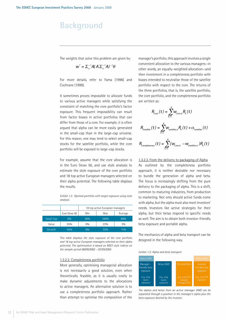
32 An EDHEC Risk and Asset Management Research Centre Publication
The EDHEC European Investment Practices Survey 2008 - January 2008
The weights that solve this problem are given by:
w* = Σεε
-1A( A'Σεε
-1A) -1θ
For more details, refer to Fama (1996) and Cochrane (1999).
It sometimes proves impossible to allocate funds to various active managers while satisfying the constraint of matching the core portfolio’s factor exposure. This frequent impossibility can result from factor biases in active portfolios that can differ from those of a core. For example, it is often argued that alpha can be more easily generated in the small-cap than in the large-cap universe. For this reason, one may tend to select small-cap stocks for the satellite portfolio, while the core portfolio will be exposed to large-cap stocks.
For example, assume that the core allocation is in the Euro Stoxx 50, and use style analysis to estimate the style exposure of the core portfolio and 18 top active European managers selected on their alpha potential. The following table displays the results.
Exhibit 1.2: Optimal portfolio with target exposure using style analysis
This table displays the style exposure of the core portfolio and 18 top active European managers selected on their alpha potential. The optimisation is based on MSCI style indices on the sample period 08/09/2002 – 07/29/2005
1.3.2.2. Completeness portfolio More generally, optimising managerial allocation is not necessarily a good solution, even when theoretically feasible, as it is usually costly to make dynamic adjustments to the allocations to active managers. An alternative solution is to use a completeness portfolio approach. Rather than attempt to optimise the composition of the
manager’s portfolio, this approach involves a single convenient allocation to the various managers—in other words, an equally-weighted allocation—and then investment in a completeness portfolio with biases intended to neutralise those of the satellite portfolio with respect to the core. The returns of the three portfolios, that is, the satellite portfolio, the core portfolio, and the completeness portfolio are written as:
RCore (t ) = wCore ,k Rk (t )
k =1
K
∑
RSatellite ( t ) = wsatellite ,k Rk (t )
k =1
K
∑ +αSatellite ( t )
RCompleteness (t ) = (wCore ,k -wSatellite ,k )Rk (t )
k =1
K
∑
1.3.2.3. From the delivery to packaging of Alpha As outlined by the completeness portfolio approach, it is neither desirable nor necessary to bundle the generation of alpha and beta. The focus is increasingly shifting from the pure delivery to the packaging of alpha. This is a shift, common to maturing industries, from production to marketing. Not only should active funds come with alpha, but the alpha must also meet investors’ needs. Investors like active strategies for their alpha, but their betas respond to specific needs as well. The aim is to obtain both investor-friendly beta exposure and portable alpha.
The mechanics of alpha and beta transport can be designed in the following way.
Exhibit 1.3: Alpha and beta transport
The alphas and betas from an active manager (AM) can be separated through a position in the manager’s alpha plus the beta exposure desired by the investor.
Background
18 top active European managers
Euro Stoxx 50 Min Max Average
Small Cap 0% 46% 100% 86%
Value 55% 0% 22% 3%
Growth 45% 0% 32% 11%
Manager-friendly beta
exposure
(e.g., long equity
exposure)
Alpha (AM)
Betas (AM)
(e.g., long equity
exposure)
Investorfriendly beta
exposure
(e.g., long TIPS exposure)
Alpha (AM)
Portable Beta
(e.g., long TIPS exposure
through ETFs)
33An EDHEC Risk and Asset Management Research Centre Publication
The EDHEC European Investment Practices Survey 2008 - January 2008
As depicted above, the alpha and beta from an active manager (AM) can be separated. The initial situation is manager beta exposure (large-cap equity) plus the alpha from the manager. Holding the beta exposure of the active manager may not correspond to the strategic allocation that the investor has defined. Implementing a beta transport can help the investor to replace all or part of the manager beta with the betas he desires. For example, the investor may be interested in acquiring exposure to inflation-protected securities (indexed US government bonds such as TIPS, for example). This exposure may correspond to his objective of protecting his portfolio from inflation. The transfer is achieved by a short position in the manager’s beta (an equity index) and a long position in the investor’s desired beta (an index for inflation-protected bonds). This beta transport can be achieved easily through ETFs of futures. Thus, the final position of the investor allows him to obtain the desired exposure to inflation-protected bonds, while benefiting from the alpha of a set of active equity managers. Indexing instruments such as ETFs, available for a wide range of asset classes and styles, can be used to neutralise manager-friendly betas and replace them with investor-friendly betas, in particular since such instruments can be sold short.
1.3.3. Dynamic core-satellite approach 1.3.3.1. Dynamic management of the tracking error budgetThe core-satellite concept essentially allows the tracking error of the overall allocation to be managed. If the investor has a tracking error budget, the target tracking error can be achieved by fixing the proportions invested in the core and in the satellite. However, management of the tracking error budget can also be done dynamically, with the proportion invested in the active portfolio varying as a function of the current cumulative out-performance, with respect to the benchmark, of the global portfolio. This objective is achieved by transporting the traditional constant proportion portfolio insurance method (CPPI) to the context of core-
satellite portfolio management, so as to allow more efficient relative risk control.
The standard CPPI procedure, introduced by Black and Jones (1987) and Black and Perold (1992), allows the production of option-like positions through systematic trading rules. This procedure dynamically allocates total assets to a risky asset in proportion to a multiple of the cushion, that is, the difference between current wealth and a desired protective floor, thus producing an effect similar to owning a put option. With such a strategy, the portfolio’s exposure tends to zero as the cushion approaches zero; when the cushion is zero, the portfolio is completely invested in cash. Thus, in theory, the guarantee is perfect: the strategy of exposure ensures that the portfolio never descends below the floor; in the event that it touches the floor, the fund is “dead”—it can deliver no performance beyond that of the guarantee.
This procedure of constant proportion portfolio insurance techniques, originally designed to ensure the respect of absolute performance, can be extended to a relative return context. Amenc, Malaise, and Martellini (2004) devise a new method allowing investors to gain full access to good tracking error, while maintaining the level of bad tracking error at a reasonable threshold, through optimal dynamic adjustment of the fractions invested in core and satellite portfolios. This method, which can be seen as a structured form of active management, appears to be a natural extension of constant proportion portfolio insurance techniques.
An approach similar to standard CPPI can be taken to offer the investor a guarantee on the relative level of performance, with a cap on under-performance with respect to the benchmark. The techniques of traditional CPPI still apply, provided that the risky asset is re-interpreted as the satellite portfolio, which contains relative risk with respect to the benchmark, and the risk-free asset is re-interpreted as the core portfolio,
Background

34 An EDHEC Risk and Asset Management Research Centre Publication
The EDHEC European Investment Practices Survey 2008 - January 2008
which contains no relative risk with respect to the benchmark.
Exhibit 1.4: Traditional CPPI versus Relative Approach CPPI
Traditional CPPI Relative Approach CPPI
Risky Asset Satellite Portfolio
Risk-free Asset Core Portfolio
This table compares the traditional CPPI to the relative approach CPPI
Let us consider an example. We assume that the benchmark is a passive investment, a bond index, for instance. The guarantee is set at 90% of the benchmark value and we assume that the multiplier is equal to 4.
At the initial date T0, portfolio value and benchmark value are normalised at 100, with a floor set at 90% of the benchmark value. The floor is thus 0.9×100 = 90. The cushion is therefore equal to 100 – 90 = 10. The investment in the satellite is then 10 × 4 = 40, which results in 100 – 40 = 60 in the core. At date T1, let us assume that the difference between the satellite and the benchmark is +10%, resulting, for example, from the following scenario: S = 0%, C = -10%. In this case, the position invested in the core has decreased by 10%, from 60 to 54. Besides, the active portfolio value has remained stable at 40, while the benchmark has also decreased by 10%, from 100 to 90. The difference between the fund value (94 = 54 + 40) and the benchmark value (90) is now equal to 4. The floor has dropped from 0.9 × 100 to 0.9 × 90 = 81. Thus, the cushion is now 94-81=13. The new optimal fraction to invest in the satellite is 13 × 4 = 52, which leaves 94 – 52 = 42 in the core portfolio. On date T1 the resulting allocation is therefore 52/94 = 55% in the satellite and 42/94 = 45% in the core portfolio.
Let us assume, on the other hand, that the difference between the satellite and the benchmark is -10%, resulting, for example, from the following scenario: S = 0%, C = +10%. In this case, the position invested in the core has increased by 10%, from 60 to 66. Besides, the
active portfolio value has remained stable at 40, while the benchmark has also increased by 10%, from 100 to 110. The floor is now at 0.9×110 = 99. The difference between the fund value (106 = 66 + 40) and the floor (99) is now equal to 7, meaning that the cushion has decreased from its initial value of 10. The new optimal fraction to invest in the satellite portfolio is 7 × 4 = 28, which leaves 106 – 28 = 78 in the core portfolio. On date T1 the resulting allocation is therefore 28/106 = 26% in the satellite and 78/106 = 74% in the core portfolio.
As can be seen from this example, the method leads to an increase in the fraction allocated to the satellite (from 40% to 55% in the example) when the satellite has outperformed the benchmark. Indeed, the accumulation of past out-performance has resulted in an increase in the cushion, and thus greater potential for a more aggressive (and hence higher tracking error) strategy in the future. If, on the other hand, the satellite has under-performed with respect to the benchmark, the method leads to a tighter tracking error strategy (through a decrease of the fraction invested in the satellite portfolio) in an attempt to ensure that the relative performance objective is met.
This approach allows dissymmetric management of tracking error; in other words, it ensures that the under-performance of the portfolio with respect to the benchmark will be limited, while giving the investor greater access to excess returns potentially generated by the active portfolio.
The benefit of this approach is that dynamic core-satellite management allows an investor to truncate the relative return distribution so as to allocate the probability weights away from severe relative under-performance and towards greater potential sources of out-performance.
When the active portfolio (the satellite) is an absolute return market-neutral fund with low levels of average risk (volatility) and extreme risks (VaR), the method can be implemented with
Background
35An EDHEC Risk and Asset Management Research Centre Publication
The EDHEC European Investment Practices Survey 2008 - January 2008
relatively high multiplier values, allowing high exposure to the benefits of positive tracking error, while limiting exposure to the dangers of negative tracking error.
1.3.3.2. Dynamic core-satellite allocationIt is usual to construct core-satellite portfolios by placing assets that are supposed to outperform the core in the satellites. During some periods, however, these assets may under-perform the core if, for example, economic conditions become temporarily unfavourable for these assets. The dynamic core-satellite approach described above makes it possible to reduce a satellite’s impact on performance during a period of relative under-performance, while maximising the benefits of the periods of out-performance.
Indeed, the observation of investors’ behaviour shows that they are not necessarily symmetric with respect to their expectations. When stock market indices perform well, they are happy to be engaged in relative return strategies. On the other hand, when stock market indices perform poorly, they express a strong desire for absolute return strategies. Techniques such as Value-at-Risk minimisation or volatility minimisation only allow symmetrical risk management. For example, due to tracking error constraints the minimum variance process leads to renunciation of part of the upside potential in the performance of commercial indices in exchange for a lower exposure to downside risk. While this strategy allows long-term out-performance, it can lead to significant short-term under-performance. It is also very hard to recover from severe market drawdown. A set of techniques involving non-linear dynamic allocation and enabling a focus on asymmetric risk management is described below.
From an absolute return perspective, it is possible to propose a trade-off between the performance of the core and satellite. This trade-off is not symmetric, as it consists of maximising the investment in the satellite when it is outperforming the core and, conversely, of minimising its weight
when it under-performs the core. The aim of this kind of dynamic allocation is to generate risk-adjusted returns in excess of those generated by static core-satellite allocation. This dynamic allocation first requires the imposition of a lower limit on under-performance with respect to the benchmark on the terminal date, i.e.,
)()( TkBTV > , where k is lower than one, e.g., k = 90%, and B(t) is the benchmark value at date t. It is then necessary to provide access to potential out-performance of the benchmark by investing in a satellite whose value on date t is denoted by S(t).
As mentioned above, Amenc, Malaise, and Martellini (2004) describe a method, known as dynamic core-satellite management, which allows asymmetric tracking error management. This method leads to an increase in the fraction allocated to the satellite when the satellite has outperformed the benchmark. Indeed, past out-performance results in an increase in the cushion, and therefore in the potential for a more aggressive (and hence higher tracking error) strategy in the future. If the satellite has under-performed with respect to the benchmark, the method leads to a tighter tracking error strategy (through a decrease of the fraction invested in the satellite portfolio) in an attempt to ensure the achievement of the relative performance objective.
This dual objective is achieved by a suitable extension of the CPPI to a relative risk management context. The concept of this process was described above. Let V(t) be the portfolio on date t. It can be broken into a floor and a cushion, according to the relation V(t) = F(t) + C(t). The floor is given by F(t) = kB(t). Take the investment in the satellite, that is, the risky asset in a relative context, to be E(t) = mC(t), with m as a constant multiplier, while the remainder of the portfolio V(t) - E(t) is invested in the benchmark.
The process for cushion growth tells us about the upside potential and allows us to calibrate an optimal value for m.
Background
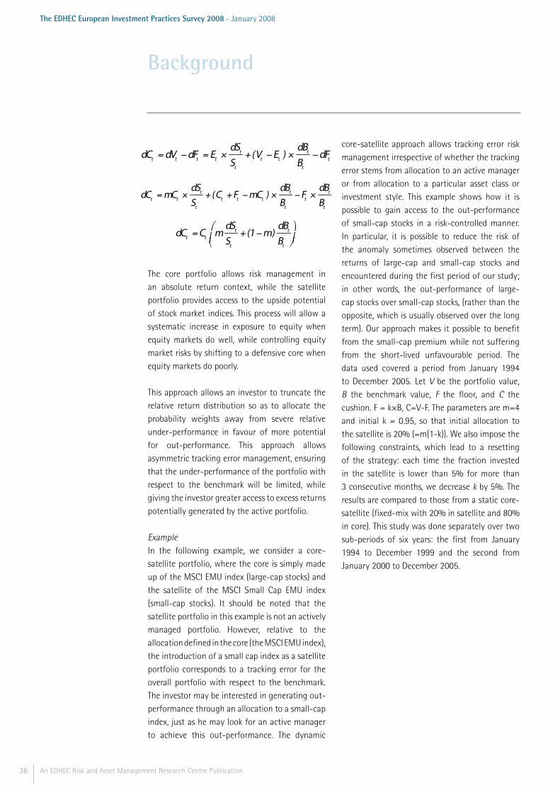
36 An EDHEC Risk and Asset Management Research Centre Publication
The EDHEC European Investment Practices Survey 2008 - January 2008
dCt = dVt - dFt = Et ×
dSt
St
+ (Vt - Et ) ×dBt
Bt
- dFt
dCt = mCt ×
dSt
St
+ (Ct + Ft - mCt ) ×dBt
Bt
- Ft ×dBt
Bt
dCt = Ct m
dSt
St
+ (1- m)dBt
Bt
⎛
⎝⎜⎞
⎠⎟
The core portfolio allows risk management in an absolute return context, while the satellite portfolio provides access to the upside potential of stock market indices. This process will allow a systematic increase in exposure to equity when equity markets do well, while controlling equity market risks by shifting to a defensive core when equity markets do poorly.
This approach allows an investor to truncate the relative return distribution so as to allocate the probability weights away from severe relative under-performance in favour of more potential for out-performance. This approach allows asymmetric tracking error management, ensuring that the under-performance of the portfolio with respect to the benchmark will be limited, while giving the investor greater access to excess returns potentially generated by the active portfolio.
ExampleIn the following example, we consider a core-satellite portfolio, where the core is simply made up of the MSCI EMU index (large-cap stocks) and the satellite of the MSCI Small Cap EMU index (small-cap stocks). It should be noted that the satellite portfolio in this example is not an actively managed portfolio. However, relative to the allocation defined in the core (the MSCI EMU index), the introduction of a small cap index as a satellite portfolio corresponds to a tracking error for the overall portfolio with respect to the benchmark. The investor may be interested in generating out-performance through an allocation to a small-cap index, just as he may look for an active manager to achieve this out-performance. The dynamic
core-satellite approach allows tracking error risk management irrespective of whether the tracking error stems from allocation to an active manager or from allocation to a particular asset class or investment style. This example shows how it is possible to gain access to the out-performance of small-cap stocks in a risk-controlled manner. In particular, it is possible to reduce the risk of the anomaly sometimes observed between the returns of large-cap and small-cap stocks and encountered during the first period of our study; in other words, the out-performance of large-cap stocks over small-cap stocks, (rather than the opposite, which is usually observed over the long term). Our approach makes it possible to benefit from the small-cap premium while not suffering from the short-lived unfavourable period. The data used covered a period from January 1994 to December 2005. Let V be the portfolio value, B the benchmark value, F the floor, and C the cushion. F = k×B, C=V-F. The parameters are m=4 and initial k = 0.95, so that initial allocation to the satellite is 20% (=m(1-k)). We also impose the following constraints, which lead to a resetting of the strategy: each time the fraction invested in the satellite is lower than 5% for more than 3 consecutive months, we decrease k by 5%. The results are compared to those from a static core-satellite (fixed-mix with 20% in satellite and 80% in core). This study was done separately over two sub-periods of six years: the first from January 1994 to December 1999 and the second from January 2000 to December 2005.
Background
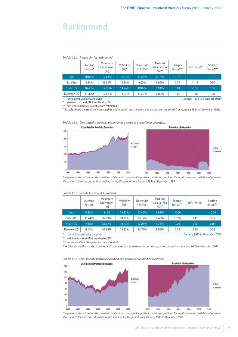
37An EDHEC Risk and Asset Management Research Centre Publication
The EDHEC European Investment Practices Survey 2008 - January 2008
Background
Average Return*
Maximum Drawdown
(%)
Volatility (%)*
Downside Risk (%)*
Modified Value-at-Risk
(%)***
Sharpe-Ratio*/**
Info-Ratio*Sortino Ratio*/**
Core 19.03% 17.84% 15.04% 11.68% 6.13% 1.13 - 1.46
Satellite 6.54% 26.81% 13.34% 9.02% 6.09% 0.34 -1.15 0.50
Static CS 16.43% 17.95% 14.24% 10.89% 5.94% 1.01 -1.19 1.32
Dynamic CS 17.30% 17.88% 14.57% 11.20% 6.03% 1.05 -1.02 1.37
Exhibit 1.5.a: Results for first sub-period
* annualised statistics are given January 1994 to December 1999** risk-free rate and MAR are fixed at 2% *** non-annualised 5%-quantiles are estimatedThis table shows the results of core-satellite optimisation, both dynamic and static, over the period from January 1994 to December 1999.
Exhibit 1.5.b: Core-satellite portfolio evolution and portfolio evolution of allocation
The graph on the left shows the evolution of dynamic core-satellite portfolio, while the graph on the right shows the evolution of portfolio allocation to the core and to the satellite, during the period from January 1994 to December 1999.
Average Return*
Maximum Drawdown
(%)
Volatility (%)*
Downside Risk (%)*
Modified Value-at-Risk
(%)***
Sharpe-Ratio*/**
Info-Ratio*Sortino Ratio*/**
Core 0.82% 54.85 19.93% 13.42% 9.63% -0.06 - -0.09
Satellite 11.44% 37.63% 18.22% 13.12% 8.40% 0.52% 1.12 0.72
Static CS 2.86% 51.72% 19.23% 13.04% 9.21% 0.04 1.08 0.07
Dynamic CS 6.12% 48.64% 18.92% 12.71% 8.95% 0.22 0.99 0.32
Exhibit 1.5.c: Results for second sub-period
* annualised statistics are given January 2000 to December 2005 ** risk free rate and MAR are fixed at 2% *** non-annualised 5%-quantiles are estimatedThis table shows the results of core-satellite optimisation, both dynamic and static, on the period from January 2000 to December 2005.
Exhibit 1.5.d: Core-satellite portfolio evolution and portfolio evolution of allocation
The graph on the left shows the evolution of dynamic core-satellite portfolio, while the graph on the right shows the evolution of portfolio allocation to the core and allocation to the satellite, for the period from January 2000 to December 2005.

38 An EDHEC Risk and Asset Management Research Centre Publication
The EDHEC European Investment Practices Survey 2008 - January 2008
2. Indices and BenchmarksOf course, in order to conduct any meaningful portfolio analysis as described in the previous section, basic building blocks reflecting the characteristics of each asset class or investment style are needed. For example, back-testing a dynamic core-satellite strategy as described above or using a multi-index model for structural covariance matrix estimation requires these building blocks. These building blocks exist in the form of indices and benchmarks and are an essential part of the investment process for most investment managers. They play a critical role in both asset allocation and performance measurement. However, benchmark selection is not always given the attention it requires. Despite the development of techniques for constructing customised benchmarks or normal portfolios reflecting the manager’s strategic asset allocation strategy, most investment managers still use simple market indices. In the following section, we take a detailed look at the role of benchmarks and indices in portfolio management; in particular, we attempt to clear up the confusion frequently surrounding the terms “benchmark” and “index”.
2.1. Indices vs. Benchmarks 2.1.1. Importance of benchmarksA benchmark is defined as a portfolio of reference and, consequently, it is supposed to be representative of the risks of the managed portfolio. It is widely accepted that the choice of benchmark plays an important role in portfolio performance. In a study whose results are often misinterpreted, Brinson, Singer, and Beebower (1991) conclude that more than 90% of the variability in portfolio returns over time is explained by the initial asset allocation. Likewise, Ibbotson and Kaplan (2000) conclude that 40% of the difference between fund returns is explained by the strategic allocation choice between the various asset classes.
Benchmark construction allows objectives to be fixed in terms of the portfolio’s systematic risk exposure, which is reflected in its strategic asset
allocation. The benchmark also serves to evaluate portfolio performance. A widespread practice in the industry is to look at a manager’s performance in relative terms—that is, with respect to a benchmark. If the portfolio management is said to be ‘benchmark-free’, the role of the benchmark is restricted to performance evaluation. But even then it is possible to derive ex post a benchmark that mimics the returns and the risk exposure of the portfolio.
2.1.2. Is a benchmark necessarily an index?An index is a portfolio that is representative of one or more risk factors. For example, a geographic index aims to be representative of the risk of the stock market of the country under consideration, while a style index and a sector index are representative of the risks of a particular investment style or industry sector. We speak of indexed management when the index is the benchmark of the portfolio. However, it is important to stress that the terms ‘indices’ and ‘benchmarks’, which are often inappropriately used as synonyms, do not mean the same thing. While an index is representative of the market as a whole or of a certain segment of the market, a benchmark must be representative of the risks chosen by an investor over the long term. Instead of simply choosing an index as a benchmark, a portfolio manager can choose to use a combination of indices or any portfolio. Therefore, even though an index can be used as benchmark, the benchmark is not necessarily an index. And using a benchmark in the investment process does not necessarily mean resorting to passive or indexed management.
2.1.3. Are indices good benchmarks?Despite numerous initiatives related to the creation of customised benchmarks or normal portfolios that reflect the allocation policy of the fund, a majority of managers choose to use an index as their benchmark. So an important question is whether indices can be considered good benchmarks. Two aspects have to be considered when answering this question. First, a benchmark must be representative of the risks
Background

39An EDHEC Risk and Asset Management Research Centre Publication
The EDHEC European Investment Practices Survey 2008 - January 2008
the portfolio is exposed to during the analysis period. If the manager decides to track an index closely, and deviates only by making specific bets (stock picking) that are different from the index, then this index can be considered an appropriate (good) benchmark. On the other hand, if the manager obtains his performance from a choice of systematic risk factors that are different from those inherent to the index, then the latter will not make a good benchmark. The second aspect to take into account is related to benchmark efficiency, which means that the benchmark is the best investment choice the investor can possibly make. This is clearly not the objective of an index, which aims to be representative of a risk. An index cannot be the optimal market portfolio, which is unobservable, as Roll (1977) explains. Indeed, the true market portfolio would have to contain all the risky assets in proportion to their market values, including assets that are not traded on markets, such as those related to human capital (salaries, stock-options, and so on).
Bailey, Richards, and Tierney (1990) and Bailey (1992) have set out rules, now commonly accepted, on the characteristics of an appropriate benchmark. A benchmark must be unambiguous, investable, measurable, and appropriate. In addition, it must reflect the investor’s current investment views, and it must be specified in advance. To respect these conditions, the managers must define a benchmark for which the risk exposure is truly reflective of the neutral or “normal” weights of their portfolio over a given period. Broad market indices do not reflect the characteristics of a managed portfolio, and are not suitable for evaluating its performance if the managed portfolio has an exposure to systematic risk factors that differs from that of the index. It is important to stress that broad market indices constitute specific choices of risk factors rather than a “neutral” risk exposure. A manager who selects a market index as a benchmark can see his risk exposure undergo modifications over time. As a result, the risk exposure may no longer correspond to the initial choices. Moreover, index
style composition is not stable over time, as shown by the following graph for the CAC40 and Euro Stoxx 50 indices.
Exhibit 21: Style composition of two equity indices
Results are based on a Sharpe (1992) RBSA style analysis over a six-month rolling period using weekly returns.
Style indices, which have been developed to respond to the growth of specialisation in portfolio management, are supposed to better reflect the characteristics of portfolios that are managed according to a specific style. However, the choice of a style index should also be considered with reservations, as there is no consensus on a single style among the various providers. The composition and construction methods of these indices differ greatly from one provider to another. As a consequence, differences in returns from one competing equity style index to another can be substantial. In addition, a generic index may not truly reflect a particular manager’s style, as there are generic indices for only some pre-defined categories. So the construction of customised benchmarks appears to be the best way of
Background
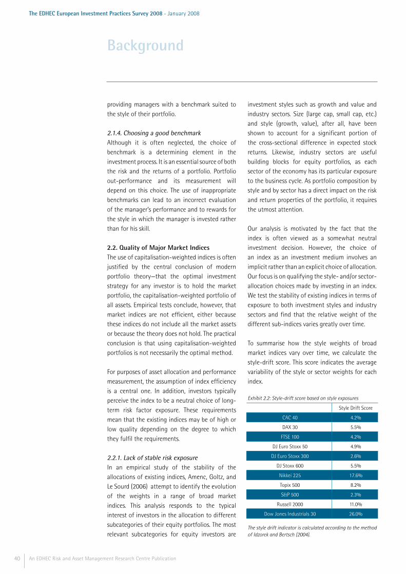
40 An EDHEC Risk and Asset Management Research Centre Publication
The EDHEC European Investment Practices Survey 2008 - January 2008
providing managers with a benchmark suited to the style of their portfolio.
2.1.4. Choosing a good benchmarkAlthough it is often neglected, the choice of benchmark is a determining element in the investment process. It is an essential source of both the risk and the returns of a portfolio. Portfolio out-performance and its measurement will depend on this choice. The use of inappropriate benchmarks can lead to an incorrect evaluation of the manager’s performance and to rewards for the style in which the manager is invested rather than for his skill.
2.2. Quality of Major Market Indices The use of capitalisation-weighted indices is often justified by the central conclusion of modern portfolio theory—that the optimal investment strategy for any investor is to hold the market portfolio, the capitalisation-weighted portfolio of all assets. Empirical tests conclude, however, that market indices are not efficient, either because these indices do not include all the market assets or because the theory does not hold. The practical conclusion is that using capitalisation-weighted portfolios is not necessarily the optimal method.
For purposes of asset allocation and performance measurement, the assumption of index efficiency is a central one. In addition, investors typically perceive the index to be a neutral choice of long-term risk factor exposure. These requirements mean that the existing indices may be of high or low quality depending on the degree to which they fulfil the requirements.
2.2.1. Lack of stable risk exposureIn an empirical study of the stability of the allocations of existing indices, Amenc, Goltz, and Le Sourd (2006) attempt to identify the evolution of the weights in a range of broad market indices. This analysis responds to the typical interest of investors in the allocation to different subcategories of their equity portfolios. The most relevant subcategories for equity investors are
investment styles such as growth and value and industry sectors. Size (large cap, small cap, etc.) and style (growth, value), after all, have been shown to account for a significant portion of the cross-sectional difference in expected stock returns. Likewise, industry sectors are useful building blocks for equity portfolios, as each sector of the economy has its particular exposure to the business cycle. As portfolio composition by style and by sector has a direct impact on the risk and return properties of the portfolio, it requires the utmost attention.
Our analysis is motivated by the fact that the index is often viewed as a somewhat neutral investment decision. However, the choice of an index as an investment medium involves an implicit rather than an explicit choice of allocation. Our focus is on qualifying the style- and/or sector-allocation choices made by investing in an index. We test the stability of existing indices in terms of exposure to both investment styles and industry sectors and find that the relative weight of the different sub-indices varies greatly over time.
To summarise how the style weights of broad market indices vary over time, we calculate the style-drift score. This score indicates the average variability of the style or sector weights for each index.
Exhibit 2.2: Style-drift score based on style exposures
Style Drift Score
CAC 40 4.2%
DAX 30 5.5%
FTSE 100 4.2%
DJ Euro Stoxx 50 4.9%
DJ Euro Stoxx 300 2.6%
DJ Stoxx 600 5.5%
Nikkei 225 17.6%
Topix 500 8.2%
S&P 500 2.3%
Russell 2000 11.0%
Dow Jones Industrials 30 26.0%
The style drift indicator is calculated according to the method of Idzorek and Bertsch (2004).
Background
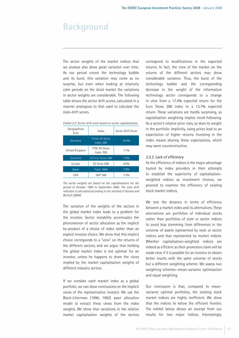
41An EDHEC Risk and Asset Management Research Centre Publication
The EDHEC European Investment Practices Survey 2008 - January 2008
The sector weights of the market indices that we analyse also show great variation over time.As our period covers the technology bubble and its burst, this variation may come as no surprise, but even when looking at relatively calm periods on the stock market the variations in sector weights are considerable. The following table shows the sector drift scores, calculated in a manner analogous to that used to calculate the style-drift scores.
Exhibit 2.3: Sector-drift score based on sector capitalisations
Geographical Zone
Index Sector Drift Score
GermanyPrime All Share
Index 38010.4%
United KingdomFTSE All Share
Index 7007.1%
Eurozone DJ Euro Stoxx 300 7.2%
Europe DJ Stoxx 600 6.6%
Japan Topix 1666 7.0%
USA S&P 500 7.3%
The sector weights are based on the capitalisations for the period of October 1995 to September 2005. The style drift indicator is calculated according to the method of Idzorek and Bertsch (2004).
The variation of the weights of the sectors in the global market index leads to a problem for the investor. Sector instability accentuates the phenomenon of sector allocation as the implicit by-product of a choice of index rather than an explicit investor choice. We show that this implicit choice corresponds to a “view” on the returns of the different sectors, and we argue that holding the global market index is not optimal for an investor, unless he happens to share the views implied by the market capitalisation weights of different industry sectors.
If we consider each market index as a global portfolio, we can draw conclusions on the implicit views of the representative investor. We use the Black-Litterman (1990, 1992) asset allocation model to extract these views from the index weights. We show that variations in the relative market capitalisation weights of the sectors
correspond to modifications in the expected returns. In fact, the view of the market on the returns of the different sectors may show considerable variation. Thus, the burst of the technology bubble and the corresponding decrease in the weight of the information technology sector corresponds to a change in view from a 17.4% expected return for the Euro Stoxx 300 index to a 13.7% expected return. These variations are hardly surprising, as capitalisation weighting implies trend-following. As a sector’s relative price rises, so does its weight in the portfolio. Implicitly, rising prices lead to an expectation of higher returns. Investing in the index means sharing these expectations, which may seem counterintuitive.
2.2.2. Lack of efficiencyAs the efficiency of indices is the major advantage touted by index providers in their attempts to establish the superiority of capitalisation-weighted indices as investment choices, we proceed to examine the efficiency of existing stock market indices.
We test the distance in terms of efficiency between a market index and its alternatives. These alternatives are portfolios of individual stocks rather than portfolios of style or sector indices to avoid bias stemming from differences in the universe of assets represented by style or sector indices and that represented by market indices. Whether capitalisation-weighted indices are indeed as efficient as their promoters claim will be made clear if it is possible for an investor to obtain better results with the same universe of stocks but a different weighting scheme. We assess two weighting schemes—mean-variance optimisation and equal weighting.
Our conclusion is that, compared to mean-variance optimal portfolios, the existing stock market indices are highly inefficient. We show that the indices lie below the efficient frontier. The exhibit below shows an excerpt from our results for two major indices. Interestingly,
Background
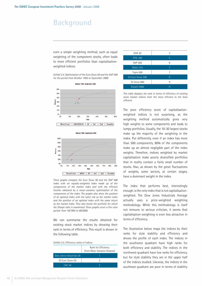
42 An EDHEC Risk and Asset Management Research Centre Publication
The EDHEC European Investment Practices Survey 2008 - January 2008
even a simple weighting method, such as equal weighting of the component stocks, often leads to more efficient portfolios than capitalisation-weighted indices.
Exhibit 2.4: Optimisation of the Euro Stoxx 50 and the S&P 500 for the period from October 1995 to September 2000
These graphs compare the Euro Stoxx 50 and the S&P 500 index with an equally-weighted index made up of the components of the market index and with the efficient frontier obtained by a mean-variance optimisation of the components of the index. The graphs also show the position of an optimal index with the same risk as the market index and the position of an optimal index with the same return as the market index. They also locate the portfolio for which the Sharpe ratio is maximised. These graphs cover a five-year period: from 10/1995 to 09/2000.
We can summarise the results obtained for existing stock market indices by showing their rank in terms of efficiency. This result is shown in the following table.
Exhibit 2.5: Efficiency ranks of indices
Rank for Efficiency
(from Mean-Variance Analysis)
Dow Jones Industrials 30 1
DJ Euro Stoxx 50 2
CAC 40 3
DAX 30 3
FTSE 100 5
S&P 500 6
Nikkei 225 7
Topix 500 7
DJ Euro Stoxx 300 9
DJ Stoxx 600 9
Russell 2000 11
This table displays the rank in terms of efficiency of existing stock market indices from the most efficient to the least efficient.
The poor efficiency score of capitalisation-weighted indices is not surprising, as the weighting method automatically gives very high weights to some components and leads to lumpy portfolios. Usually, the 10-30 largest stocks make up the majority of the weighting in the index. Put differently, even if an index has more than 500 components, 90% of the components make up an almost negligible part of the index weights. Therefore, indices weighted by market capitalisation make poorly diversified portfolios that in reality contain a fairly small number of stocks. Also, as shown by the great fluctuations of weights, some sectors, at certain stages, have a dominant weight in the index.
The index that performs best, interestingly enough, is the only index that is not capitalisation-weighted. The Dow Jones Industrials Average actually uses a price-weighted weighting methodology. While this methodology is itself not immune to serious criticism, it seems that capitalisation-weighting is even less attractive in terms of efficiency.
The illustration below maps the indices by their ranks for style stability and efficiency and shows the profile of each index. The indices in the southwest quadrant have high ranks for both efficiency and stability. The indices in the northwest quadrant have low ranks for efficiency, but for style stability they are in the upper half of the indices studied. Likewise, the indices in the southeast quadrant are poor in terms of stability
Background
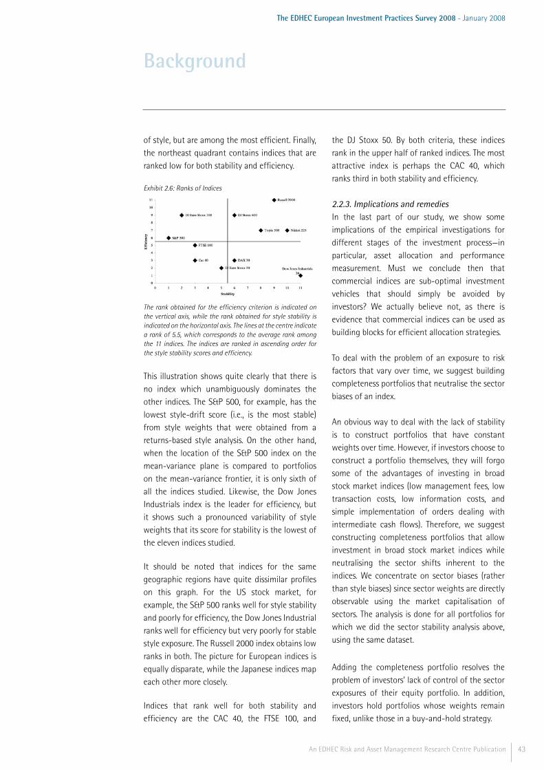
43An EDHEC Risk and Asset Management Research Centre Publication
The EDHEC European Investment Practices Survey 2008 - January 2008
of style, but are among the most efficient. Finally, the northeast quadrant contains indices that are ranked low for both stability and efficiency.
Exhibit 2.6: Ranks of Indices
The rank obtained for the efficiency criterion is indicated on the vertical axis, while the rank obtained for style stability is indicated on the horizontal axis. The lines at the centre indicate a rank of 5.5, which corresponds to the average rank among the 11 indices. The indices are ranked in ascending order for the style stability scores and efficiency.
This illustration shows quite clearly that there is no index which unambiguously dominates the other indices. The S&P 500, for example, has the lowest style-drift score (i.e., is the most stable) from style weights that were obtained from a returns-based style analysis. On the other hand, when the location of the S&P 500 index on the mean-variance plane is compared to portfolios on the mean-variance frontier, it is only sixth of all the indices studied. Likewise, the Dow Jones Industrials index is the leader for efficiency, but it shows such a pronounced variability of style weights that its score for stability is the lowest of the eleven indices studied.
It should be noted that indices for the same geographic regions have quite dissimilar profiles on this graph. For the US stock market, for example, the S&P 500 ranks well for style stability and poorly for efficiency, the Dow Jones Industrial ranks well for efficiency but very poorly for stable style exposure. The Russell 2000 index obtains low ranks in both. The picture for European indices is equally disparate, while the Japanese indices map each other more closely.
Indices that rank well for both stability and efficiency are the CAC 40, the FTSE 100, and
the DJ Stoxx 50. By both criteria, these indices rank in the upper half of ranked indices. The most attractive index is perhaps the CAC 40, which ranks third in both stability and efficiency.
2.2.3. Implications and remediesIn the last part of our study, we show some implications of the empirical investigations for different stages of the investment process—in particular, asset allocation and performance measurement. Must we conclude then that commercial indices are sub-optimal investment vehicles that should simply be avoided by investors? We actually believe not, as there is evidence that commercial indices can be used as building blocks for efficient allocation strategies.
To deal with the problem of an exposure to risk factors that vary over time, we suggest building completeness portfolios that neutralise the sector biases of an index.
An obvious way to deal with the lack of stability is to construct portfolios that have constant weights over time. However, if investors choose to construct a portfolio themselves, they will forgo some of the advantages of investing in broad stock market indices (low management fees, low transaction costs, low information costs, and simple implementation of orders dealing with intermediate cash flows). Therefore, we suggest constructing completeness portfolios that allow investment in broad stock market indices while neutralising the sector shifts inherent to the indices. We concentrate on sector biases (rather than style biases) since sector weights are directly observable using the market capitalisation of sectors. The analysis is done for all portfolios for which we did the sector stability analysis above, using the same dataset.
Adding the completeness portfolio resolves the problem of investors’ lack of control of the sector exposures of their equity portfolio. In addition, investors hold portfolios whose weights remain fixed, unlike those in a buy-and-hold strategy.
Background
44 An EDHEC Risk and Asset Management Research Centre Publication
The EDHEC European Investment Practices Survey 2008 - January 2008
These completeness portfolios not only have more stable sector exposure, but also achieve more favourable performance in terms of risk and return. Thus, investors seeking the most attractive risk-return profile for their portfolio could benefit from implementing a simple neutralisation strategy by holding a global index and a completeness portfolio made up of sector indices. In the same vein, for purposes of performance measurement, investors can use a combination of indices to construct benchmarks that are more sophisticated than a global index. Such a benchmark is often called a “customised benchmark”, to emphasise that it is not simply a global index.
The fact that global indices show a pronounced lack of efficiency is probably the most interesting result of this study. The remedy we proposed for the asset allocation phases of the investment process is to construct efficient portfolios; it is possible to do so, for example, from sector indices. These sector indices can be used in an optimisation procedure that makes it possible to avoid the drawbacks of the global indices. The approach we proposed makes it possible to avoid estimation risk by focusing on the minimum risk portfolio and shows significant enhancement of efficiency in an out-of-sample exercise.
Our results show that the volatility of the minimum-variance portfolio is always significantly lower than that of the corresponding market index. It is important to note that this lower volatility is not achieved by construction and that the portfolios can actually be obtained ex ante by an investor.
It is striking that, for five out of six indices, the lower risk of the minimum-variance portfolio does not lead to a lower expected return. The minimum-variance portfolio of sectors that make up the S&P 500 index is the sole exception. All other minimum-variance portfolios have higher expected returns than the corresponding index. Consequently, except for the S&P 500,
the Sharpe ratios are considerably higher than those of the market index.
While these findings show that commercial indices pose serious challenges for an investor who wishes to use them in the investment process, they do not necessarily mean that an investor should not use indices at all. Quite to the contrary, as we have shown that there are straightforward remedies for the problems of commercial stock market indices. All of these solutions are based on indices that reflect finer sub-segments of the equity market, such as investment styles or industry sectors. The main drawback of global stock market indices may actually be that rather than allow a precise and explicit definition of the asset allocation they imply a somewhat confused allocation by sub-segment. Sector indices and style indices seem to be appropriate tools that allow investors to gain control over the investment process while focusing on its most rewarding phase—the asset allocation decision.
2.3. Innovation in the Index World2.3.1. Alternatives to value-weighted indicesWhen constructing indices, the two main issues are the inclusion criteria for stocks and the weighting scheme. The choice of the index sample universe involves the choice of the number and type of assets to put in the index. An example of a narrow-based market index is the Dow Jones Industrial Averages, which is made up of 30 stocks. At the other extreme, the New York Stock Exchange index contains every share listed on the New York Stock Exchange. Index weighting is the second important factor in constructing indices. The choice of an appropriate weighting system makes it possible to produce acute and investable benchmarks in line with investment management. For several years, researchers have been examining alternatives to conventional capitalisation weighting.
Background

45An EDHEC Risk and Asset Management Research Centre Publication
The EDHEC European Investment Practices Survey 2008 - January 2008
First, we review some of the papers that propose alternative construction methodologies. Second, we will provide some insights into industry adoption of these alternatives.
2.3.1.1. Overview of alternative indexing techniquesThe main idea behind alternative weighting mechanisms is that indices that are constructed differently may outperform capitalisation weighted market indices for a number of reasons.
These include:(i) Use of better allocation techniques(ii) Access to additional risk premia(iii) Exposure to undervalued securities and exploitation of market inefficiencies
Differences to capitalisation weighting are twofold:(i) The weighting criterion is different from the market capitalisation.(ii) Strategies may not be buy-and-hold.
Price weightingPrice-weighted indices are computed by averaging the prices of the assets that make up the indices. The drawback of this method is that assets with low unit values have less weight in the index than assets with high unit values. Moreover, it does not take asset capitalisation and trading volumes into account. The advantages are that computation and interpretation are simple.
This type of index is evaluated in the following way:
It =
1n
Piti =1
n
∑divisort
where n is the number of assets in the index and
itP is the price of asset i at the time the index is computed. The divisor is an adjustment term that makes it possible to express the index as a percentage with respect to a date of reference. This formulation allows us to adjust the index by recalculating the divisor, in the event of fluctuations in the capital of the firm.
The most well known price-weighted index, and the first to have been set up, is the Dow Jones Index Average. The Nikkei index in Japan is price-weighted as well. Because of the way they are calculated, these indices are not suited to an evaluation of the performance of a stock exchange. Indeed, these indices are more affected by the price variations of assets with high unit values than those of assets with low unit values. Moreover, as they are made up of a restricted number of assets, they are also unsuited to an evaluation of the performance of diversified portfolios.
Equal weightingEqually-weighted indices are the average of the returns of their components. They give the same importance to the price movements of all the stocks they are made up of, so the price change of every company in the index has the same impact on the changing value of the index. Each stock has an equal influence on index performance, regardless of its market capitalisation or share price.
An index that has equal weights for each of the components may be associated with a contrarian strategy. Whether the capitalisation of a company rises or falls, its weight in the index will remain constant. Therefore, the weights of winners (losers) are lower (higher) than with capitalisation weighting. Aside from evolution over time, even at the outset equally weighted indices will have greater weights in small capitalisation stocks than will capitalisation weighted indices, which naturally underweight small stocks. When small cap-stocks are earning a premium, equally-weighted indices will likewise earn higher returns.
It has also been claimed that equally-weighted indices are less risky than their capitalisation-weighted counterparts, since the method of capitalisation weighting leads to high concentration in a few stocks that have the highest market capitalisation. Wei and Zhang (2006) use the CRSP data to compare the volatility
Background
46 An EDHEC Risk and Asset Management Research Centre Publication
The EDHEC European Investment Practices Survey 2008 - January 2008
of capitalisation-weighted and equally-weighted indices. They find that the volatility of the equally-weighted index is higher than the volatility of the capitalisation-weighted index, a finding that they ascribe to the overweighting of the more volatile small-cap stocks.
The major problem with equally-weighted portfolios is that equal weighting holds only for an infinitely short period, since the weights will diverge from equal weighting if the components have returns that differ. The geometric mean index of stock prices has been shown to grow at the same rate as a portfolio that is equally weighted and rebalanced in continuous time (see Rothstein 1972 and 1974 or Hodges and Schaefer 1974). However, Brennan and Schwartz (1985) have shown that this equal rate of growth is true only if the rate of return on individual stocks is stochastic. Even in this case, however, the geometric mean index approximates the returns on the continuously rebalanced portfolio.
Southard and Bond (2003) note that the use of equal weighting instead of capital weighting is not an optimal solution as it does not result in a representative portfolio. The second limitation of conventional indices described by Southard and Bond is that the stocks selected for the indices are not evaluated for performance. Stocks are placed in the index regardless of their investment value, creating embedded valuation risk when used as investable portfolios. According to these authors, when indices are used as investment media, it is necessary to evaluate their potential components before selecting them for the index. However, it should also be noted that this critique by Southard and Bond implicitly advocates the selection of stocks from valuation principles rather than constructing representative indices, which does not seem to be a convincing suggestion (see below for more comments on such weighting methods).
Geometric mean The standard procedure for calculating an index is prices multiplied by weights summed over the
stock population of the index and divided by the number of stocks to produce an arithmetic mean.
Geometric-mean indices provide an alternative. These indices are related to the group of equally-weighted indices, as they do not take asset capitalisation into account. Price relatives of the stocks included are multiplied over all stocks and the n-th root is taken from the product thus obtained.
It = It -1
Pit
Pit -1i =1
n
∏n
An example of a geometric-mean index is the Value Line Index. It is in fact the only one. The advantage of this index is that it does not depend on asset prices, but on their relative variation.
According to Cootner (1972), a geometric-mean index is, unlike an arithmetic-mean index, a downward-biased index of price changes. On the other hand, other authors underline that while arithmetic-mean indices are sensitive to the selection of the time interval (monthly, quarterly, semi-annual, or annual) in the model, geometric indices will produce the same calculation of returns regardless of the time interval.
Stochastic portfolio theory and diversity-weighted indexingFernholz and Shay (1982) introduce a continuous-time equilibrium model that focuses on the long-term performance of stock portfolios. Their contribution is to characterise equilibrium, not by using the classic concept of market clearing between supply and demand, but by using notions of equilibrium borrowed from the field of thermodynamics. They show that there are portfolios that allow equilibrium to be attained and that are different—and possibly even very different—from the market portfolio. The theory has been applied to portfolio management and performance analysis, most notably by INTECH, which introduced diversity-weighted indexing (Fernholz, Garvy, and Hannon 1998). Diversity-
Background

47An EDHEC Risk and Asset Management Research Centre Publication
The EDHEC European Investment Practices Survey 2008 - January 2008
weighted indexing is based on a measure of stock market diversity that is provided by the distribution of capital in a given stock market. The measure of diversity is:
Dp = ϖi
p
i =1
N
∑⎛
⎝⎜⎞
⎠⎟
1
p
where N is the number of stocks, p is a constant between zero and one and is fixed to 0.76 in the proposed diversity-weighted index, and iϖ is the market-cap weight of the i th stock. It can be shown that the returns on the diversity-weighted index are a function of the returns on a capitalisation-weighted index with the same component stocks. Returns on the diversity-weighted index will exceed those on the capitalisation-weighted index unless diversity is continuously declining or the dividends paid out by large companies significantly exceed those paid out by small company stocks.
Factor analysis Factor-analysis techniques have been extensively used in finance, both in the context of term-structure analysis (a classic reference is Litterman and Sheinkman 1991) as well as in the time-series analysis of equity portfolios (Chan, Karceski, and Lakonishok 1998, among others). In the context of empirical testing of the arbitrage pricing theory (Ross 1976), replicating portfolios are extracted in an attempt to track the performance of the unobserved implicit factors that drive asset returns (see Huberman, Kandel, and Stambaugh 1987).
The intuitive aim of the technique is to use a small sample of stocks to design a replicating portfolio for the return of the total stock market. To this end, the selection criterion is the loading of individual stocks on the first principal component. The higher the loading of a stock on the first principal component, the higher its contribution to the common trend in stock returns will be. Given that the first eigenvector corresponding to the first principal component is determined so as to maximise the variance of the corresponding
linear combination of stock returns, high factor loadings will be allocated to stocks which have been highly correlated with the total stock market over the calibration period. These stocks should be the most representative. This allocation ensures compliance with requirements for both representativity and investability (the necessity of having a small number of stocks).
Alexander and Dimitriu (2003) suggest obtaining portfolio weights from a principal component analysis of stock returns. Their model filters out the noise by focusing on replicating the common trend in stock returns, as described by the first principal component. This process allows them to significantly outperform capitalisation-weighted benchmarks while maintaining high correlation with the latter. They attribute this out-performance to exposure to the value and volatility premia. Affleck-Graves, Troskie, and Money (2002) note that the trouble with the use of principal components in the construction of stock market indices is that it often results in the allocation of negative weights to some of the securities. The authors show that, by a simple restatement of the problem, this disadvantage is easily overcome. In addition, extra constraints can be imposed, if so desired, on the weights assigned to the different securities.
The foundations of the construction of stock market indices based on a principal components analysis are to be found in Feeney and Hester (1964). The intuition is that if an index is designed to measure movement on the market, then it will be most sensitive (and hence most informative) if the weights are assigned in such a way that the index has a maximum variance over all linear combinations of the stocks to be included in the index. This combination is simply the largest principal component.
The problem of getting positive weightings can be solved with any of the methods for solving either general non-linear programming problems (for example, the flexible tolerance
Background
48 An EDHEC Risk and Asset Management Research Centre Publication
The EDHEC European Investment Practices Survey 2008 - January 2008
method) or quadratic programming problems subject to quadratic constraints. One of the main advantages of the flexible tolerance method is that it is easy to include additional constraints in the analysis. Since the flexible tolerance method is an iterative search procedure, Himmelblau (1972) recommends that the analysis be repeated using several different starting solutions. As it results in somewhat more computation than the traditional principal component analysis, it is suggested that in practice the traditional first principal component be found. If it is non-negative and satisfies all of the additional restrictions imposed, then these weights should be used. However, if the requirements are not satisfied, then the flexible tolerance method should be used to find the index that is the most volatile, subject to the imposed requirements.
Weighting by fundamental metrics Arnott, Hsu, and Moore (2004) create market indices in which they change the weighting criterion from market capitalisation to other observable characteristics of the stocks. They use indices composed of 100 stocks that are weighted by variables such as firm size, book value, income, sales, gross dividend distributions, number of employees, etc. It should be noted that all of these variables proxy for firms, but by using a measure that is different from market capitalisation and thus more closely related to the physical size of the firm than to the value of shareholders’ equity. Southard and Bond (2003) define what they call intelligent indices, i.e., indices that select their securities for their capital appreciation potential rather than simply incorporating representative securities regardless of their investment merit. Risk management of intelligent indices is primarily controlled through a representative sampling portfolio optimisation process. A simpler method of portfolio optimisation is to combine assets whose specific risks offset each other. Stratified sampling divides the universe along the dimensions of sector and size and then forces the model to pick a proportionate number of stocks from each of these groups.
This optimisation controls the exposure of “intelligent” indices to these segments of the market; ultimately, it also manages the risk of the index and the tracking error with respect to other widely used benchmarks. According to the authors, the important implication of this portfolio construction process is that it provides an accurate and representative portfolio while diversifying the stock-specific risk found in more conventional indices. Securities are selected using a multifactor approach, allowing the model to incorporate all relevant information factors. The methodology evaluates securities across a wide range of investment value factors which can be broken down into four perspectives: fundamental growth, stock valuation, timeliness, and risk determinates. Each perspective is intended to bring an independent viewpoint to the stock valuation process. Over the long-term, indices based on selecting and weighting stocks according to attributes of the firm have been shown to outperform value-weighted indices, but a lively debate has broken out in the industry, with critics arguing that these indices are just value-tilted active strategies that outperform value-weighted indices over past periods but may suffer when value investing is out of favour (see Asness 2006).
2.3.1.2. Adoption of alternative indexing techniquesIntrigued by the obvious shortcomings of value-weighted indices and the emergence of alternative indexing techniques, EDHEC issued a call for reactions to investment professionals on the perception and use of indices. The answers of the more than eighty respondents (asset management firms, pension funds, insurance companies, private banks, etc.) reinforce the view that the criticism of value-weighted indices is widely shared within the industry.
Although it would at first appear that the majority of respondents are not, in general, dissatisfied with the indices they use as benchmarks (18.82% of respondents express
Background

49An EDHEC Risk and Asset Management Research Centre Publication
The EDHEC European Investment Practices Survey 2008 - January 2008
degrees of dissatisfaction), further examination soon reveals that the shortcomings of these indices, such as inefficiency, lack of stability, and susceptibility to price bubbles, are widely recognised by the industry professionals responding to the survey. The results also show that a considerable majority of respondents plan to review the indices they use as benchmarks, either immediately or in the future.
Overall, responses to the call for reactions suggest that, in some ways, industry practices reflect the concerns over the quality of stock market indices. Nearly 70% of the respondents, after all, indicate that they use customised benchmarks and other indices in an attempt to compensate for the flaws inherent to the use as benchmarks of such indices as the CAC 40, the S&P 500, the DAX 30, the FTSE 100, or the Dow Jones Industrials 30. It is clear then that, for a significant majority of investors, the choice of benchmark is a fundamental choice. In the end, the name of the index provider, the volumes managed, turn out to matter less than such attributes as the efficiency of the index, its stability, its immunity to bubbles, or its risk exposure.
The questionnaire begins by asking whether practitioners are satisfied with the indices they use as benchmarks. Our motivation for this question is to see whether practitioners are aware of the shortcomings of existing stock market indices. And, as it turns out, stock market industries do generate considerable dissatisfaction. Although 10.59% and 32.94% of the 85 respondents who answer this question choose “very satisfied” and “fairly satisfied” respectively, 37.65% choose not to make a decisive statement, and a total of 18.82% reply that they are dissatisfied (“fairly dissatisfied” or “very dissatisfied”).
An interesting question is why only a minority of respondents express satisfaction with the existing indices. The EDHEC study concludes that cap-weighted indices have two main drawbacks—inefficiency and a lack of stability. The replies
to a question asking whether the respondents share this view suggest that these conclusions are convincing. After all, the majority (67.06% of the 85 who answer this question) state that they share EDHEC’s opinion of cap-weighted indices; 20% disagree and 12.94% choose no response. Consequently, we can safely say that the inefficiency and lack of stability of cap-weighted indices are well recognised problems for the practitioners who replied to our call for reactions.
Exhibit 2.7: Are you satisfied with the indices you use as benchmarks?
Exhibit 2.8: Do you share EDHEC’s opinion of cap-weighted indices?
For a finer distinction as to which problems with the existing stock market indices are perceived as the most severe, we ask what bothers respondents most about cap-weighted indices.
Background
Very satisfied
Fairly satisfied
Neither satisfied or dissastisfied
Fairly dissastisfied
Very dissastisfied
32.94%
37.65%
3.53% 10.59%
15.29%
Yes
No
No response
67.06%20.00%
12.94%

50 An EDHEC Risk and Asset Management Research Centre Publication
The EDHEC European Investment Practices Survey 2008 - January 2008
73 survey participants respond to this question. To all appearances, inefficiency is the most serious problem, as it is mentioned by 65.75% of respondents. Lack of stability was chosen by 38.36%. 17.81% of respondents bring up other problems. 4.11% believe that the cap-weighted indices are susceptible to price bubbles and fads. 6.85% of respondents suggest problems such as return drag, momentum strategies, free-float issues, lack of history, and incompleteness. The remainder (6.85%) of respondents state that nothing bothers them. One particularly noteworthy result is that although a total of 43.53% of the 85 respondents insist that they are very or fairly satisfied with the indices they use as benchmarks, only 5.88% of these respondents say nothing bothers them about the use of indices as benchmarks. This result lends support to the view that, while indices are widely accepted and their quality unquestioned, most practitioners are able to make out some drawbacks once specific questions are asked.
Exhibit 2.9: What bothers you about cap-weighted indices?
Given the perceived drawbacks, a natural question is to ask whether respondents use indices that are not cap-weighted. 69.41% of the 85 respondents affirmed that they do. 54.24% of those who answer this question say they use a customised benchmark with an optimal combination of sector or style indices. These responses reveal that most investors agree with the remedy proposed in the
EDHEC study, which recommends using style analysis to construct customised benchmarks. A further 35.59% of those who answer this question choose equal-weighted indices, and 23.73% choose fundamental indices. 11.86% of respondents say that they use other kinds of benchmarks. 3.39% use a benchmark comprised of various indices and 5.08% construct benchmarks from other factors. A further 3.39% adopt liability-oriented benchmarks, such as the inflation rate plus 5%. It is only to be expected that most of the users of composite benchmarks (comprised of various indices or other components) are asset management companies, while all of the liability-oriented benchmark users are pension funds or insurance companies.
Exhibit 2.10: If you use a benchmark other than cap-weighted indices, please specify what it is.
When asked whether they intend to review the indices currently in use, 38.10% of the 84 investment professionals who respond to this question say they will review them soon and 42.86% say they intend to review them in the future. Only 19.05% of respondents say they have no plans to do so. Obviously, the limitations of the indices currently in use are well recognised.
Background
Ineffiency
Lack of stability
Other
0%
10%
20%
30%
40%
50%
60%
70%
80%
65.75%
38.36%
17.81%
Customised benchmark using an optimal combinaison of sector or style indices
Equal-weighted indices
Fundamental indices
Other (e.g., composite benchmarks, inflation rate +5%, absolute return)
0%
10%
20%
30%
40%
50%
60%
54.24%
35.59%
23.73%
11.86%
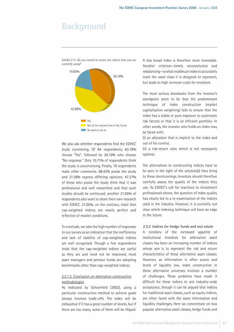
51An EDHEC Risk and Asset Management Research Centre Publication
The EDHEC European Investment Practices Survey 2008 - January 2008
Exhibit 2.11: Do you intend to review the indices that you are currently using?
We also ask whether respondents find the EDHEC study convincing. Of 84 respondents, 63.10% choose “Yes”, followed by 26.19% who choose “No response.” Only 10.71% of respondents think the study is unconvincing. Finally, 19 respondents make other comments: 68.42% praise the study and 31.58% express differing opinions. 47.37% of those who praise the study think that it was professional and well researched and that such studies should be continued; another 21.05% of respondents also want to share their own research with EDHEC. 21.05%, on the contrary, insist that cap-weighted indices are nearly perfect and reflective of market conditions.
To conclude, we take the high number of responses to our survey as an indication that the inefficiency and lack of stability of cap-weighted indices are well recognised. Though a few respondents insist that the cap-weighted indices are useful as they are and need not be improved, most asset managers and pension funds are adopting benchmarks other than cap-weighted indices.
2.3.1.3. Conclusion on alternative construction methodologiesAs indicated by Schoenfeld (2002), using a particular construction method to achieve goals always involves trade-offs. The index will be exhaustive if it has a great number of stocks, but if there are too many, some of them will be illiquid.
A less broad index is therefore more investable. Another criterion—timely reconstitution and rebalancing—is what enables an index to accurately track the asset class it is designed to represent, but leads to high turnover costs for investors.
The most serious drawbacks from the investor’s standpoint seem to be that the predominant technique of index construction (market capitalisation weighting) fails to ensure that the index has a stable or pure exposure to systematic risk factors or that it is an efficient portfolio. In other words, the investor who holds an index may be faced with:(i) an allocation that is implicit to the index and out of his control;(ii) a risk-return ratio which is not necessarily optimal.
The alternatives to constructing indices have to be seen in the light of the solution(s) they bring to these shortcomings. Investors should therefore carefully assess the quality of the indices they use. As EDHEC’s call for reactions to investment professionals shows, the question of index quality has clearly led to a re-examination of the indices used in the industry. However, it is currently not clear which indexing technique will have an edge in the future.
2.3.2. Indices for hedge funds and real estate A corollary of the increased appetite of institutional investors for alternative asset classes has been an increasing number of indices whose aim is to represent the risk and return characteristics of these alternative asset classes. However, as information is often scarce and levels of liquidity low, index construction in these alternative universes involves a number of challenges. These problems have made it difficult for these indices to win industry-wide acceptance, though it can be argued that indices for traditional asset classes, such as equity indices, are often faced with the same information and liquidity challenges. Here we concentrate on two popular alternative asset classes, hedge funds and
Background
Yes
Not at the moment but in the future
No plans to do so
38.10%
42.86%
19.05%

52 An EDHEC Risk and Asset Management Research Centre Publication
The EDHEC European Investment Practices Survey 2008 - January 2008
real estate, and review in turn some of the issues arising with index construction for these classes.
2.3.2.1. Problems with hedge fund indices Hedge fund indices have seen widespread growth over the past few years, reflecting both the general growth of the hedge fund industry and the strengthening position of indices over other investment vehicles, such as funds of funds. The interest in indices is mainly driven by institutional investors, who have a strong preference for low-fee, transparent and risk-controlled investments.
Different data, different selection criteria, and different methods are used to construct the available indices. The result, unsurprisingly, is that competing indices for the same strategy have different returns (see Brooks and Kat 2002 or Amenc, Martellini, and Vaissié 2004). Investors can hardly rely on these contradictory sources of information for a “true and fair” view of hedge fund performance. One of the reasons for this lack of homogeneity in hedge fund index return data is that none of these existing indices is fully representative. Because hedge funds are not obliged to disclose performance, existing databases cover only a relatively small fraction of the hedge fund population.
Hedge fund indices are built from databases of individual fund returns, and therefore inherit their shortcomings in terms of scope and quality of data, shortcomings that vary greatly from one data vendor to another. Below, we briefly review the biases hedge fund indices are known to suffer from. First, a fund’s participation in a database is voluntary, which poses a real problem in terms of the reliability of the data published (“self-reporting bias”). Since the funds that have refused to report to a database are, by definition, unobservable, it is not possible to evaluate the impact of this bias. In addition, since some refuse to display their performance because of poor results and others because they have already reached their critical size, it is difficult to know even whether this bias has a positive or negative
impact on performance. Also, depending on the date at which the database begins, the quality of past information will vary (especially for funds that ceased their activity before the database began). This variation in information affects the performance of some indices more than that of others, depending on how many of the funds that make up the index stop communicating their results each year (referred to as the attrition rate) and on the average performance differential observed between those funds and the remaining funds. This is known as a “survivorship bias”. Brown, Goetzmann, and Ibbotson (1999) value the average impact of this bias at 2.6%, compared to 3% for Fung and Hsieh (2000), and 2.43% for Liang (2001). For mutual funds, by comparison, Malkiel (1995) estimates this bias to be 0.5%. Also, the database providers have selection criteria that can be very diverse, and the data provided will not be representative of the same management universe. This is referred to as "selection bias." When a fund is added to a database, all or part of its historical data is recorded ex post in the database. Since the databases are the sole means of communication for most funds, it is reasonable to believe that the funds, to attract as many investors as possible, will decide to publish their results only when they are at their highest levels. It is therefore probable that the average performances displayed by the funds during their incubation period will be better than those of funds that have belonged to the database under consideration for a longer period. In this case, we talk about "instant history bias” or “backfill bias”. Fung and Hsieh (2001) value the impact of this bias at 1.4 % per year, but a study by Posthuma and Van der Sluis (2003) estimates the actual average backfill bias to be 4.35%.
These problems of representativity and of database biases have led to severe doubts about the usefulness of hedge fund indices. Fung and Hsieh (2004) note that current hedge fund indices provide broad indicators of the health of the industry, but few specific answers to questions of
Background
53An EDHEC Risk and Asset Management Research Centre Publication
The EDHEC European Investment Practices Survey 2008 - January 2008
asset allocation and performance measurement. Likewise, because of the problems outlined above, regulators have inquired into the appropriateness of hedge fund indices as eligible assets for retail investment products (Committee of European Securities Regulators 2006). For much the same reason, many investors have also taken a critical stance on hedge fund indices.
We examine below whether the problems that are outlined for hedge fund indices also exist for other indices that seem to be widely accepted. Our conclusion is that the limitations of hedge fund indices pointed out in the literature do indeed exist. However, we point out that there are possible solutions to these problems. We argue as well that most of the problems are not specific to hedge fund indices, but also affect well accepted instruments such as stock market indices. Therefore, rejecting hedge fund indices is inconsistent with the treatment of indices for other asset classes that are subject to the same problems. For all these reasons, it would be regrettable if investors and regulators rejected all hedge fund indices,12 without distinguishing between those that are in fact quality indices and those that use the term “index” for marketing reasons alone.
It should also be noted that there are various types of hedge fund indices and that they can be classified along two lines. The first distinction is between non-investable and investable indices. There actually seems to be some confusion between investable and non-investable indices among investors, as many problems underlined in the literature (notably the data biases) apply mainly to non-investable indices and are less severe for investable indices. It is surprising that many investors insist on the problems of database biases with non-investable indices as outlined in the literature, when the only indices actually relevant for investment decisions are the investable indices. The second distinction is between strategy indices for a particular hedge fund style or strategy and global hedge fund indices that aggregate funds across
all investment styles. The construction of representative indices is far more feasible for strategy indices, which may attain representativity for a given style, than it is for global indices, which cannot claim to be truly representative of the entire hedge fund universe.
In section 2.3.2.3, we assess some of the problems of hedge fund indices by looking at the case of stock market indices. The objective is to see whether similar problems arise with stock market indices or whether—on the contrary—the problems really are limited to the area of hedge funds. But, first, we will outline methods for constructing quality hedge fund indices, and then we will address each problem.
2.3.2.2. Innovative solutions While hedge fund indices based on large databases come with a large number of biases linked to the construction of the database itself, it should also be stressed that such indices are—by definition—not investable. In response to this problem, numerous investable hedge fund indices have been created. Our suggestion would be to prefer investable indices, since these indices avoid a number of database problems associated with non-investable indices. However, in addition to the low number of funds used by investable indices, providers of investable hedge fund indices often use the questionable practice of selecting the index components for their good performance in the past, a practice that leads to indices that are not at all representative of the entire hedge fund universe for a given strategy. Therefore, it must be made clear that these investable indices are also representative. While it may not be straightforward—what with the requirement for investability—to ensure representativity, recent research shows that designing hedge fund indices that are both investable and representative is entirely feasible.
Goltz, Martellini, and Vaissié (2007) examine how modern portfolio theory and factor-analysis techniques can be used to build investable, yet
Background
12 - In Europe, hedge fund indices have struggled to win acceptance from the industry and from regulators. A survey of market participants (EDHEC 2005) finds that investors largely prefer funds of hedge funds to indices when implementing hedge fund allocations (see pp. 82, 83). The Committee of European Securities Regulators (2006) adopted a critical stance on hedge fund indices at the beginning of a consultation process undertaken in an attempt to establish whether hedge fund indices should be eligible to serve as underlying securities for index derivatives used by retail investment funds.
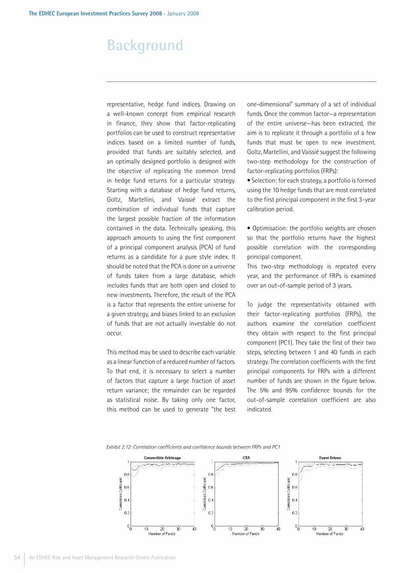
54 An EDHEC Risk and Asset Management Research Centre Publication
The EDHEC European Investment Practices Survey 2008 - January 2008
representative, hedge fund indices. Drawing on a well-known concept from empirical research in finance, they show that factor-replicating portfolios can be used to construct representative indices based on a limited number of funds, provided that funds are suitably selected, and an optimally designed portfolio is designed with the objective of replicating the common trend in hedge fund returns for a particular strategy. Starting with a database of hedge fund returns, Goltz, Martellini, and Vaissié extract the combination of individual funds that capture the largest possible fraction of the information contained in the data. Technically speaking, this approach amounts to using the first component of a principal component analysis (PCA) of fund returns as a candidate for a pure style index. It should be noted that the PCA is done on a universe of funds taken from a large database, which includes funds that are both open and closed to new investments. Therefore, the result of the PCA is a factor that represents the entire universe for a given strategy, and biases linked to an exclusion of funds that are not actually investable do not occur.
This method may be used to describe each variable as a linear function of a reduced number of factors. To that end, it is necessary to select a number of factors that capture a large fraction of asset return variance; the remainder can be regarded as statistical noise. By taking only one factor, this method can be used to generate "the best
one-dimensional" summary of a set of individual funds. Once the common factor—a representation of the entire universe—has been extracted, the aim is to replicate it through a portfolio of a few funds that must be open to new investment. Goltz, Martellini, and Vaissié suggest the following two-step methodology for the construction of factor-replicating portfolios (FRPs):• Selection: for each strategy, a portfolio is formed using the 10 hedge funds that are most correlated to the first principal component in the first 3-year calibration period.
• Optimisation: the portfolio weights are chosen so that the portfolio returns have the highest possible correlation with the corresponding principal component. This two-step methodology is repeated every year, and the performance of FRPs is examined over an out-of-sample period of 3 years.
To judge the representativity obtained with their factor-replicating portfolios (FRPs), the authors examine the correlation coefficient they obtain with respect to the first principal component (PC1). They take the first of their two steps, selecting between 1 and 40 funds in each strategy. The correlation coefficients with the first principal components for FRPs with a different number of funds are shown in the figure below. The 5% and 95% confidence bounds for the out-of-sample correlation coefficient are also indicated.
Background
Exhibit 2.12: Correlation coefficients and confidence bounds between FRPs and PC1

55An EDHEC Risk and Asset Management Research Centre Publication
The EDHEC European Investment Practices Survey 2008 - January 2008
As can be seen from the figure, the out-of-sample correlations with the first principal component are very robust with respect to the number of funds in the FRP. Even when only five to ten funds are used, correlations are very high. On the other hand, choosing more than ten funds does not significantly increase the correlation. The only case where correlation drops considerably when selecting fewer than ten funds is the Equity Market Neutral FRP.
2.3.2.3. Are these problems specific to hedge funds? In the following paragraphs we list the problems encountered with hedge fund indices and compare them with those of market indices.
RepresentativityIn fact, a lack of representativity is not necessarily specific to hedge fund indices. It has often been noted that the mechanism of capitalisation-weighting often used in stock market indices actually results in portfolios that are not representative of the entire market (see Strongin, Petsch, and Sharenow 2000); they find that the effective number of stocks in cap-weighted indices is low compared to the actual number of constituent stocks in the index). In addition, some widely accepted indices contain only a small number of stocks in the first place. As a result, even the widely accepted stock market indices provide but a limited representation of the universe of traded stocks.
Differences in returns from one provider to anotherIt appears that equity style indices are as heterogeneous as hedge fund strategy indices (Amenc and Goltz 2006). The degree of heterogeneity is important in magnitude. For example, an investor using the S&P index to assess February 2001 returns for value stocks would have observed a return of -11.1% while an investor using the FTSE index would have observed a return of -3.3%, a difference of 7.8 percentage points in the monthly return. So, we conclude that the problem of representativity is not limited to hedge fund indices. In fact, even equity style indices that seem to be well established as underlyings for indexing products have a low degree of representativity.
Differences in style composition from one provider to anotherThe figure below shows the strategic allocation to investment styles of US stock market indices. The style exposures are calculated using Sharpe’s returns-based style analysis for the Dow Jones IA, the S&P 500, the Russell 1000, the Russell 3000, the Wilshire 5000, and the NASDAQ-100. The style exposures are with respect to the returns of MSCI style indices for the U.S., that is, MSCI Growth, Value, and Small Cap indices, and are calculated using monthly data from January 2004 to December 2006. The results are compared with the strategic allocation to investment styles of global hedge fund indices (taken from Lhabitant 2007).
Background
The correlation coefficients are represented as a function of the number of funds included in the FRP.Source: Goltz, Martellini, and Vaissié (2007)

56 An EDHEC Risk and Asset Management Research Centre Publication
The EDHEC European Investment Practices Survey 2008 - January 2008
Exhibit 2.13: Strategic style allocation of broad stock market indices and global hedge fund indices.
It is clear that the heterogeneous style composition that is often described as a serious problem for hedge fund indices is also present in stock market indices. In fact, when it comes to style composition, it turns out that they are no less heterogeneous than hedge fund indices.
Component-weighting methodThe definition of a weighting scheme is often cited as a problem for hedge fund indices. Differences in the weights attributed to components can lead to significant differences in index performance. But choosing a weighting mechanism is problematic whatever the asset class. There are standards for equity indices, but different weighting schemes are available. First, while most indices use capitalisation weighting, additional criteria such as sales/revenue and net income are often taken into account (see “Guide to the Dow Jones Global Titan 50 Index”, January 2006). Second, capitalisation weighting has been the target of fierce criticism (see Haugen and Baker 1991, Amenc, Goltz, and Le Sourd 2006, or Hsu 2006), much of which points out that the mechanics of capitalisation weighting lead to trend-following strategies and, ultimately, an inefficient risk-return trade-off.
Alternative weighting schemes mentioned in section 2.3.1, such as attribute-weighted (Arnott, Hsu, and Moore 2005), “diversity”-weighted (Fernholz, Garvy, and Hannon 1998), or equal-weighted indices, lead to considerable differences in the performance of equity indices (see Arnott, Hsu, and Moore 2005), just as with hedge fund indices.
Selection bias (component selection)As mentioned above, the literature takes great care to spell out the sources of selection bias of hedge fund indices. Indeed, most hedge fund index providers have principles that they use to select funds for their databases and thus to construct their indices. The problem is exacerbated for investable hedge fund indices. It should be noted that providers of stock market indices commonly
Background
Value
54%
50%
42%
16%
42% 62%
<1%
38%
42%
12%
45%46%
4%
46%
68%
32%
S&P 500
Broad Stock Market Indices
DJIA
HFRX
Global Hedge Fund Indices
MSCI
S&P CS/Tremont
Dow Jones RBC
Russell 1000 Russell 3000
Wilshire 5000 Nasdaq 100
Growth Small Cap
Arbitrage Long/Short Equity Trading
48% 38%
14%
47%
22%
31%
22%
21%
57%
16%
36%48%
83%
17%
67%11%
22%

57An EDHEC Risk and Asset Management Research Centre Publication
The EDHEC European Investment Practices Survey 2008 - January 2008
have selection criteria for index components as well. Ranaldo and Häberle (2006) show that a considerable share of index-related investment management, which is usually considered passive investment management, can in fact hide a form of active management. In addition, some of the “fundamental” weighted indices actually conduct stock selection in addition to changing the weighting scheme. Any index that involves discretionary decisions by an index committee is susceptible to inherent selection biases. This problem is hardly unique to hedge fund indices.
Component transparencyReplication of hedge fund indices may be difficult, as it is not clear what their components are. Full transparency, however, is not always a given for stock market indices either, especially when these indices are constructed from proprietary databases. So, a lack of transparency is not a drawback to hedge fund indices alone.
Diversification A problem often invoked when discussing sufficient diversification of hedge fund indices is the low number of components of these indices, the investable indices, in particular. To analyse once again whether the low number of components is a problem solely for hedge fund indices, we compare the number of components of some investable hedge fund indices to that of a selection of equity indices. We find that the number of components of investable hedge fund indices is actually in the range of that of the major stock market indices, those with the largest shares of the European market (the Dow Jones IA, CAC40 Euro Stoxx 50, FTSE 100). Therefore, most investors in traditional index funds, exchange-traded funds, or stock index futures are actually exposed to narrow indices that may not fully represent the entire stock market. Defunct fundsThe problem of defunct funds affects only non-investable hedge fund indices, which are based on large databases of hedge fund returns. However,
these indices do not underlie actual investment products, as it is not feasible to invest in the large number of funds that the index contains. Therefore, the only indices that could potentially be used in the context of actual investment decisions are investable hedge fund indices, which, to allow investability, typically rely on a small number of funds. It should be noted that the actual track record of such investable indices corresponds to the true returns that investors holding the index have earned and, in this sense, they are free of any backfilling or survivorship bias.
The omission of assets, moreover, is a generic problem with any index: blaming hedge fund indices for failing to include certain funds would be akin to blaming stock market indices for not including stocks that have been delisted or stocks that are to be listed in the future! It appears that even the leading stock market indices reserve the right to exclude “poor performing” or defunct companies. While it is of great interest to require high standards of index providers in dealing with data issues such as these, it is not clear why hedge fund indices should be treated any differently from other indices in terms of regulatory requirements.
2.3.2.4 Real estate indices Indices whose aim is to reflect the risk and return characteristics of this asset class are computed by a range of index providers. As with hedge fund indices, the lack of liquidity and the scarcity of available information on property prices are considerable impediments to index construction. Recently, several real estate indices have been vying to underlie the budding US property derivatives markets. Here, we provide a brief overview of the issues with both appraisal-based and transaction-based indices. RepresentativityReal estate indices too are beset by representativity problems. Indices tracking the performance of listed property should not be regarded as representative of institutional
Background

58 An EDHEC Risk and Asset Management Research Centre Publication
The EDHEC European Investment Practices Survey 2008 - January 2008
investment in real estate, which takes place predominantly on the private market. Inclusion criteria for listed property indices focus on free-float market capitalisation and on the liquidity of real estate securities and no attempt is made to select and weight components for an index that would be representative of institutional investment practices in terms of investment styles or sectors. Likewise, international indices of listed property companies are constructed without regard for the economic weight of regions; as a result, countries with developed listed real estate sectors or large property companies are overweighted while those without are underweighted. Indices built on appraisal values contributed by institutional investors sample from a significantly larger population and need not suffer from these limitations.
DiversificationReal estate indices, like hedge fund or stock market indices, often suffer from insufficient diversification. While commercial property indices computed from the appraisal values of thousands of real estate assets and hedonic indices constructed from large numbers of transactions in the housing market appear to be sufficiently diversified, the same cannot be said of indices based on the share prices of companies investing in property. In spite of the rapid growth of the listed real estate market, it currently represents but a fraction of the overall investable property universe. As a result of the uneven development of traded real estate markets, regional indices for traded real estate suffer from problems of geographic representativity. In addition, domestic indices suffer from insufficient diversification even in highly developed markets, as few companies typically account for the bulk of the index.
Problems with appraisal-based indicesValuations and appraisals determine the capital appreciation component of a number of real estate indices. These indices are referred to as “appraisal-based” indices. The use of appraisals is warranted by the limited number of transactions
that can be observed in the private and illiquid commercial property markets: properties are typically appraised much more frequently than they are transacted. There are multiple problems revolving around the appraisal process; first, as appraisals are costly and time-consuming, they may be undertaken at a lower frequency than that of reporting—that is, contributors may revalue their properties at longer set intervals and when it is felt that value has been altered significantly. When these updates occur at intervals greater than the reporting interval, the database contains stale appraisals. The presence of stale appraisals will result in lagged and auto-correlated index returns and artificially lowered index volatility and correlations with other assets, a phenomenon known as returns smoothing.
Assuming that multiple contributors choose to adjust their valuations marginally or to leave them unchanged for several reporting periods before they undertake in-depth appraisal exercises, often clustered in the same quarter, there could then be discernible seasonality in the index, on top of the smoothing and lagging. This seasonal bias may artificially increase quarterly volatility and lower the reported annual return if it is compounded. Second, any appraiser has to work with the information available—on direct real estate markets, very little data is contemporaneous and therefore appraisers must rely on lagged market indicators and recent and not-so-recent information about transactions and appraisals of comparable properties. Appraisers may update values conservatively and wait for early market signals to be confirmed. Because of the nature of the appraisal process, appraisal-based indices will trail market prices in up and down markets. Third, aggregation of property appraisals that take place over the full course of a quarter will lead to additional smoothing of the index.
Unsmoothing appraisal-based indicesThe use of smoothed real estate data in asset management and asset-liability management exercises results in upwardly biased allocations
Background
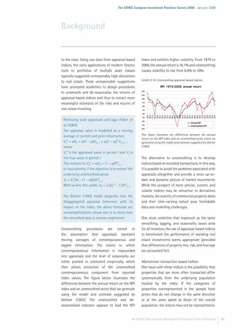
59An EDHEC Risk and Asset Management Research Centre Publication
The EDHEC European Investment Practices Survey 2008 - January 2008
to the class. Using raw data from appraisal-based indices, the early applications of modern finance tools to portfolios of multiple asset classes typically suggested unreasonably high allocations to real estate. These unreasonable suggestions have prompted academics to design procedures to unsmooth and de-seasonalise the returns of appraisal-based indices and thus to extract more meaningful estimates of the risks and returns of real estate investing.
Removing stale appraisals and lags—Fisher et al. (2003)The appraisal value is modelled as a moving average of current and prior information: Vt* = αVt + α(1 – α)Vt–1 + α(1 – α)2 Vt–2 … where Vt* is the appraised value in period t and Vt is the true value in period t This reduces to Vt* = αVt + (1 – α)V*t–1or equivalently, if the objective is to extract the underlying unsmoothed series:Vt = Vt*/α – (1 – α)/αV*t–1With α=0.4, this yields: Vt = 2.5Vt* – 1.5V*t–1
The Geltner (1993) model elegantly links the disaggregated appraisal behaviour with its impact on the index; the above formulae are oversimplifications whose aim is to show how the smoothed data is reverse-engineered.
Unsmoothing procedures are rooted in the assumption that appraisals represent moving averages of contemporaneous and lagged information. The extent to which contemporaneous information is impounded into appraisals and the level of seasonality are either posited or estimated empirically, which then allows extraction of the unsmoothed contemporaneous component from reported index values. The figure below illustrates the differences between the annual return on the NPI index and an unsmoothed series that we generate using the model and estimate suggested by Geltner (1993). The unsmoothed and de-seasonalised indicator appears to lead the NPI
index and exhibits higher volatility. From 1979 to 2006, the annual return is 10.1% and unsmoothing causes volatility to rise from 6.4% to 10%.
Exhibit 2.14: Unsmoothing appraisal-based indices.
This figure illustrates the differences between the annual return on the NPI index and an unsmoothed series which we generated using the model and estimate suggested by Geltner (1993).
The alternative to unsmoothing is to develop indices based on recorded transactions. In this way, it is possible to avoid the problems associated with appraisals altogether and provide a more up-to-date and dynamic picture of market movements. While the prospect of more precise, current, and volatile indices may be attractive to derivatives markets, the scarcity of commercial property deals and their time-varying nature pose formidable data and modelling challenges.
One must underline that inasmuch as the same smoothing, lagging, and seasonality issues arise for all investors, the use of appraisal-based indices to benchmark the performance of standing real estate investments seems appropriate (provided that differences of property mix, risk, and leverage are accounted for).
Mainstream transaction-based indicesOne issue with these indices is the possibility that properties that are more often transacted differ systematically from the underlying population tracked by the index. If the categories of properties overrepresented in the sample have prices that do not change in the same direction or at the same speed as those of the overall population, the indices may not be representative.
Background

60 An EDHEC Risk and Asset Management Research Centre Publication
The EDHEC European Investment Practices Survey 2008 - January 2008
Empirical evidence confirms the existence of this systematic sample-selection bias, but studies have suggested that its impact on indices may be limited.
The characteristics of the properties that are transacted may also differ from one period of time to another, with resulting complications for the measurement and interpretation of observed price trajectories. Buyers and sellers—and their motivations—may be different at different stages of the cycle, resulting in non-random variation in the bias. This behaviour is empirically confirmed, although studies do not find the bias to significantly influence indices.
Finally, liquidity will not be constant over time in a regular transaction price series, as it is positively correlated with the real estate cycle: rising property markets are associated with a shortening of the average time on the market and an increase in the volume of transactions, while the opposite is true of falling markets; in other words, raw transaction prices reflect not only property-specific characteristics, but also market-wide liquidity, which has a significant bearing on indices.
While transaction-based indices aim to better track the market by avoiding the appraisal-induced lag and smoothing effects, all methods suffer from sample-bias (although the extent to which they seek to address variations in quality and liquidity differs), and none fully addresses the temporal lag issue, as lag is introduced by the aggregation of transactions taking place at different times.
Conclusion on Real Estate IndicesCurrently, there is a great diversity of indices. In addition, these indices are vying to underlie investment media such as property derivatives, competition that creates difficulties as well as opportunities. The wealth of offers and diversity of indices could cause confusion among investors. But diversity could also offer value for
investors, who would be in a position to select the combination of offers that best corresponds to their needs. A potential benefit could be that the increasing number of indices and their different construction methodologies will lead to greater emphasis on the construction methodologies of real estate indices and on the quality of these indices, emphasis that cannot but spur further innovation in the use of indices as benchmarks for performance measurement.
3. Asset-Liability ManagementOne of the major conclusions of part 2 is that benchmarks play an important role in the entire investment process. In addition, we have argued that by no means should a benchmark be equated with an index. Instead, the benchmark should reflect the long-term risk/return trade-off chosen for a portfolio. For investors facing liability-constraints, these constraints essentially structure the way risk is defined. Standard indices that focus on the evolution of a typical portfolio of assets have a very weak link, if they have one at all, to the evolution of the actual liabilities. On the other hand, liabilities may be reflected by proxies for the bond markets and inflation, but more often than not a specific component of liabilities remains unaccounted for. The question facing investors who are subject to liability constraints is how, given the structure of their liabilities, to optimally manage their assets. In practice, their investment management practices should therefore differ tremendously from those of investors such as mutual funds, which are typically not concerned with liabilities. In this section, we present an overview of ALM and provide a theory for this investment approach that allows us to classify existing ALM approaches as equivalents to common asset management techniques.
3.1. A Brief History of ALMWe present a (brief) history of ALM techniques from both a practical and an academic perspective.
Background
61An EDHEC Risk and Asset Management Research Centre Publication
The EDHEC European Investment Practices Survey 2008 - January 2008
3.1.1. ALM from a practitioner’s perspectiveFrom a practical standpoint, ALM-type management techniques can be put into several categories.
A first technique, known as cash-flow matching, involves ensuring a perfect static match between the cash flows from the portfolio of assets and the commitments in the liabilities. Suppose, for example, that a pension fund has a commitment to pay out a monthly pension to a retired person. Leaving aside the complexity relating to the uncertain life expectancy of the retiree, the structure of the liabilities is defined simply as a series of cash outflows to be paid, the real value of which is known today, but for which the nominal value is typically indexed to inflation. It is possible, in theory, to construct a portfolio of assets whose future cash flows will be identical to this structure of commitments. Doing so—assuming such securities are available on the market—would involve purchasing inflation-linked zero-coupon bonds with a maturity corresponding to the dates on which the monthly pension instalments are paid out, at amounts that are proportional to the amount of real commitments.
This technique, which has the advantage of simplicity and, in theory, allows perfect risk management, nevertheless has a number of drawbacks. First of all, it will generally be impossible to find inflation-linked securities whose maturity corresponds exactly to the liability commitments. Moreover, most inflation-linked securities pay out coupons, a practice that leads to the problem of reinvesting the coupons. To the extent that perfect matching is not possible, there is a technique called immunisation, which allows the residual interest rate risk created by the imperfect match between the assets and liabilities to be managed in a dynamic way. This technique for the management of interest rate risk can be extended beyond a simple duration-based approach to fairly general contexts, including hedging larger changes in interest rates (through the introduction of a convexity
adjustment) and non-parallel shifts in the yield curve (Fabozzi, Martellini, and Priaulet 2005), or to simultaneous management of interest rate risk and inflation risk (Siegel and Waring 2004). It should be noted, however, that it is difficult to use this technique to hedge non-linear risks stemming from the presence of options hidden in the liability structures and/or to hedge non-interest rate related risks in liability structures.
Another and probably greater disadvantage of the cash-flow matching technique (or of the approximate matching version achieved by immunisation) is that it represents a position in the risk/return space that is extreme and not necessarily optimal. In fact, we can say that the cash-flow matching approach in asset-liability management is the equivalent of investing in the risk-free asset in an asset management context. It allows perfect management of the risks, namely a capital guarantee in the passive management framework, and a guarantee that the liability constraints are respected in the ALM framework. However, the lack of return, related to the absence of risk premia, makes this approach very costly and leads to an unattractive level of contribution to the assets.
To improve the profitability of the assets, and therefore to reduce the contributions, it is necessary to introduce asset classes (stocks, government bonds, and corporate bonds) which are not perfectly correlated with the liabilities into the strategic allocation. One then finds the best possible compromise between the risk (relative to the liability constraints) thereby taken on and the excess return that the investor can hope to obtain through the exposure to rewarded risk factors. Different techniques are then used to optimise the surplus—that is, the value of the assets in excess of that of the liabilities—in a risk/return space. In particular, it is useful to turn to stochastic models that allow representation of the uncertainty relating to a set of risk factors that impact the liabilities. These can be financial risks (inflation, interest rate, stocks) or non-financial
Background

62 An EDHEC Risk and Asset Management Research Centre Publication
The EDHEC European Investment Practices Survey 2008 - January 2008
risks (demographic, in particular). When necessary, agent behaviour models are then developed to represent the impact of exercising certain implicit options. For example, a policyholder can (typically in exchange for penalties) cancel his/her life insurance contract if the guaranteed contractual rate drops significantly below the interest rate prevailing at a date following the signature of the contract, which makes the amount of liability cash flows, and not just their current value, dependent on interest rate risk.
It is also appropriate to mention non-linear risk-profiling management techniques, the goal of which is to provide a compromise between a risk-
free and return-free approach on the one hand, and a risky approach that does not allow the liability constraints to be guaranteed on the other (see exhibit 3.1 for an overview of ALM techniques and the corresponding techniques in asset management). In particular, it involves introducing options which allow (partial) access to the risk premia of stocks without all of the associated risks, or dynamic allocation methods, inspired by the portfolio insurance techniques transposed into an ALM framework (see in particular Leibowitz and Weinberger (1982, 1983) for the contingent optimisation technique, or Amenc, Malaise, and Martellini (2004) for a generalisation of the dynamic core-satellite approach).
Background
Finally, following recent changes in accounting standards and regulations that have led to an increased focus on liability risk management, a new technique, referred to as liability-driven investment (LDI), has emerged, and it has quickly drawn the attention of pension funds, insurance companies, and investment consultants alike. Essentially, these standard changes force institutional investors to value their liabilities at market rates (mark-to-market) instead of at fixed discount rates, a change that results in an increase in the volatility of the liability portfolio. As a result, to reduce the volatility of their funding ratios, as required by stricter solvency rules, institutional investors must increase their focus on risk management. Although they may vary significantly from one provider to
another, LDI techniques typically involve a hedge of the duration and convexity risks via seven standard building blocks, while keeping some assets free for investing in higher yielding asset classes.
These techniques may or may not involve leverage, depending on the institutional investor’s risk aversion. When no leverage is used, a fraction of the assets (known as the liability-matching portfolio) is allocated to risk management, while another fraction of the assets is allocated to performance generation. This technique can actually be seen as a combination of two strategies, involving investing in immunisation strategies (for risk management) as well as investing in standard asset management solutions (for
Exhibit 3.1: Investment Management Approaches in Asset Management and their Counterparts in Asset-Liability Management
Risk/Return Profile Asset Management
(absolute risk)Asset-Liability Management
(relative risk)
Zero risk - no access to risk premia Investment in Risk-free assetCash-flow matching and/or
immunization
Optimal risk-return trade-offOptimally diversified portfolio
of risky assetsOptimisation of the surplus
Fund separation theoremCapital market line
(static mix of cash and optimal performance-seeking risky portfolio)
LDI solution(static mix of cash, liability matching portfolio and optimal risky portfolio)
Dynamic and skewed risk management(non linear payoffs)
Portfolio insurance(dynamic mix of risk-free asset
and optimal risky portfolio)
Dynamic LDI(dynamic mix of liability-hedging
portfolio and performance generating portfolio)
This table gives an overview of ALM techniques and the corresponding techniques in asset management

63An EDHEC Risk and Asset Management Research Centre Publication
The EDHEC European Investment Practices Survey 2008 - January 2008
performance generation). This approach stands in sharp contrast to more traditional surplus optimisation methods, where both objectives (liability risk management and performance generation) are pursued simultaneously in an attempt to achieve the portfolio with the highest possible relative risk/relative return ratio. When leverage is used, it can be explicit, in the form of a short position in the risk-free asset, or implicit, in the form of leverage induced by the use of derivatives (typically interest rates and/or inflation swaps) in the liability-matching portfolio. This use of leverage has more potential for performance generation. For example, we could take a stylised example where derivatives are used to match the liability portfolio so that virtually 100% of the assets are still available for
the performance-generation portfolio. It should be noted that the performance target for this “risky” portfolio then becomes the risk-free rate, legitimising the use of absolute return portfolios (hedge funds, capital-guaranteed products, etc.).
We actually argue below that this allocation approach, expressed in terms of allocation to three building blocks (cash, liability-matching portfolio, and performance portfolio), as opposed to allocation to standard asset classes, is consistent with a three-fund separation theorem that extends standard results from modern portfolio theory to situations involving the presence of liability constraints, and constitutes a first step toward improved asset-liability management.
Background
13 - Sources: http://www.aberdeen-asset.com/aam.nsf/institutional/fixedldi;http://www.blackrockinvestments.ch/sesite/institutional-investors/inv-sol/liability-led.htm;http://www.prnewswire.com/cgi-bin/stories.pl?ACCT=104&STORY=/www/story/06-14-2006/0004380486&EDATE;http://www.ftam.com/wps/wcm/connect/resources/file/eb894d422196968/FS_LDI_063007.pdf?MOD=AJPERES; http://www2.goldmansachs.com/client_services/asset_ma-nagement/institutional/ldi/index.html; http://www.morganstanley.com/about/press/articles/87.html; http://www.epn-magazine.com/news/fullstory.php/aid/2281/Morgan_Stanley_considers_the_merits_of_Dutch_and_German_launches_for_LDI_funds.html; http://www.ssga.com/uk/featu-res/liability_driven_investing.html; http://uk.standardlifeinvestments.com/content/press/press_releases/standard_life_investments_laun-ches_liability_managed_cre-dit_funds.html; http://www.ubs.com/1/e/globalam/gis/alis/alis_pro-ducts_us.html
Overview of current offers of LDI products13
Several actors in the institutional market offer liability-driven investment solutions (LDIs). Since assets and liabilities consist different asset classes there is different interest rate sensitivity on the two sides of the balance sheet. The main objective of most LDIs is to match liabilities. The products can be classified (see exhibit 3.2) as cash-flow matching, duration matching, surplus optimisation and/or tailored LDI strategies. The information that can be found about LDIs on the providers’ websites is scant, as most of these products are tailor-made for institutional investors.
Provider Products Description Categorisation
Aberdeen Asset Management
Fixed Income Alpha Funds Actively-managed portfolios of global fixed income securities constructed to generate above average returns overlaid by a tailored derivative-sourced duration strategy
Duration Matching,Surplus Optimisation
BlackRock -'Narrow’ Approach (high performance bond, portable alpha solutions, cash flow and duration matched bond solutions)-‘Broad’ Approach (traditional multi-asset target return investing, alternative assets and focus/unconstrained funds)
The products try to align the fund’s asset and liabilities and offer different products for different desired level of extra return on top of this covered liabilities.
Duration Matching,Surplus Optimisation
Fifth Third Asset Management
Liabilty-Driven Investment (LDI) Strategies
The LDI strategy is the process of identifying liability streams and matching those streams with incoming cash flows from investment assets that offer a superior risk/reward profile to meet those obligations and is managed to outperform custom benchmark.
Tailored LDI Strategies
Exhibit 3.2: Classification of LDI Offerings

64 An EDHEC Risk and Asset Management Research Centre Publication
The EDHEC European Investment Practices Survey 2008 - January 2008
3.1.2. ALM from an academic perspectiveWhile it seems that a priori a variety of techniques are available to institutions seeking to manage their asset portfolios in the face of their liability constraints, it remains to be seen what academic results, if any, point to the optimality of these techniques. The existing contributions to the academic literature take two different and somewhat competing approaches to ALM.
On the one hand, several authors attempt to cast the ALM problem in a continuous-time framework, and extend Merton’s inter-temporal selection analysis (Merton 1969, 1971) to account for the presence of liability constraints in the asset allocation policy. A first step in the application of optimal portfolio selection theory to the problem of pension funds was taken by Merton (1990) himself, who studies the allocation decision of a
university that manages an endowment fund. In a similar spirit, Boulier et al. (1995) formulate a continuous-time dynamic programming model of pension fund management. It contains all of the basic elements for modelling dynamic pension fund behaviour and analytical methods can be used to solve it. Rudolf and Ziemba (2004) extend these results to the case of a time-varying opportunity set, where state variables are interpreted as currency rates that affect the value of the pension’s asset portfolio. Also related is a paper by Sundaresan and Zapatero (1997), which is specifically aimed at asset allocation and retirement decisions in the case of a pension fund. This continuous-time stochastic-control approach to ALM is appealing for its tractability and simplicity, desirable because they allow full and explicit understanding of the mechanisms affecting the optimal allocation strategy.
Background
Goldman Sachs Asset Management
- Immunisation-Extended Duration- Portable Alpha- Total Portfolio Solution
Depending on the client’s liability streams, current funded status, risk tolerance and return objectives different approaches can be offered.
Tailored LDI strategies
Morgan Stanley Investment Management
Liability-Driven Investment (LDI) Alpha Plus funds
Three components are combined: interest rate & inflation risk management, uncorrelated alpha generation and protection against rising interest rates
Tailored LDI Strategies
Principal Global Investors
- Immunisation- Yield Curve Segmentation- Duration Extending- Customised Precise Liability Matching- Derivatives Overlay and Portable Alpha Strategies
A broad array of liability-based investment solutions ranging from high quality long-duration bond portfolios to customised asset portfolios that match plan liabilities is offered.
Duration Matching,Surplus Optimisation
State Street Global Advisers
Pooled Asset Liability Matching Solution (PALMS)
Investment pools that aim to help plan sponsors manage exposure to changes in interest rates and inflation
Cash-Flow Matching,Surplus Optimisation
Standard Life Investments
Liability Managed Credit Funds This product is designed to meet a pension scheme's unique needs by tailoring a mix of funds to suit each individual scheme within a single pooled bond fund.
Tailored LDI strategies
UBS Global Asset Management
ALIS (Asset Liability Investment Solutions)
These products are long duration commingled funds and mimic the sensitivity of the liabilities to changes in interest rates as well as the slope and shape of the yield curve.
Duration Matching
65An EDHEC Risk and Asset Management Research Centre Publication
The EDHEC European Investment Practices Survey 2008 - January 2008
Background
On the other hand, because of the simplicity of the modelling approach, these continuous-time models do not allow a full and realistic account of the uncertainty facing institutions in the context of asset-liability management. A second strand of the literature has therefore focused on developing more comprehensive models of uncertainty in an ALM context. Work by Kallberg et al. (1982), Kusy and Ziemba (1986), or Mulvey and Vladimirou (1992) has led to the development of a stochastic programming approach to ALM. This strand of the literature is relatively close to industry practice, with one of the first successful commercial multistage stochastic programming applications appearing in the Russell Yasuda Kasai model (Cariño et al. 1994, Cariño and Ziemba 1998). Other successful commercial applications include the Towers Perrin-Tillinghast ALM system of Mulvey et al. (2000), the fixed-income portfolio management models of Zenios (1995) and Beltratti et al. (1999), and the InnoALM system of Geyer et al. (2001). A good number of applications in asset-liability management are provided in Ziemba and Mulvey (1998) and Ziemba (2003). In most cases, stochastic programming models require the uncertainties to be approximated by a scenario tree with a finite number of states of the world at each time. Important practical issues such as transaction costs, multiple state variables, market incompleteness (uncertainty in liability streams that is not spanned by existing securities), taxes and trading limits, regulatory restrictions, and corporate policy requirements can be handled within the stochastic programming framework. On the other hand, this solution comes at the cost of tractability. Analytical solutions are not possible, and stochastic programming models need to be solved via numerical optimisation. In an attempt to circumvent concerns about the back-box flavour of stochastic programming models, some interesting attempts have been made to test for the optimality of various rule-based strategies (Mulvey et al. 2005).
3.2. A Formal Model of ALM and the LDI Approach More specifically, we introduce in this section a formal continuous-time model of asset-liability management. Note that we do not provide proofs, which may be found in Amenc, Martellini, and Ziemann (2007). This continuous-time stochastic control approach to ALM is appealing in spite of its highly stylised nature because it leads to a tractable solution, allowing a full and explicit understanding of the mechanisms affecting the optimal allocation strategy. In particular, we argue that the three-fund separation theorem we obtain, typical of optimal asset allocation decisions in the presence of a stochastic state variable, is a parsimonious way to capture some of the complexity involved in optimal investment decisions.
We let [0,T] denote the (finite) time span of the economy, where uncertainty is described through a standard probability space (Ω,A,P) and endowed with a filtration Ft ; t ≥ 0{ } , where
F∞ ⊂ A and 0F is trivial, representing theP-augmentation of the filtration generated by the n-dimensional Brownian motion
W1,...,W n( ) .
3.2.1. Stochastic model for asset pricesWe consider n risky assets, the prices of which are given by:
dPt
i = Pti μi dt + σij dWt
j
j =1
n
∑⎛
⎝⎜⎞
⎠⎟, i =1,...,n
We shall sometimes use the shorthand vector notation for the expected return (column) vector
μ = μi( ) '
i =1 ,....,nand matrix notation
σ = σij( )
i , j =1 ,....,nfor the asset return variance-
covariance matrix. We also denote 1=(1,…,1)’ an n-dimensional vector of ones and by
W = W j( ) '
j =1 ,....,nthe vector of Brownian motions.
A risk-free asset, the 0th asset, is also traded in the economy. The return on this asset, typically a default-free bond, is given by
dPt0 = Pt
0rdt , where r is the risk-free rate in the economy.
(1)

66 An EDHEC Risk and Asset Management Research Centre Publication
The EDHEC European Investment Practices Survey 2008 - January 2008
We assume that r, μ and σ are progressively measurable and uniformly bounded processes, and that σ is a non-singular matrix that is also progressively measurable and bounded uniformly.14 For some numerical applications below, we will sometimes treat these parameter values as constant.
Under these assumptions, the market is complete and arbitrage-free and there exists a unique equivalent martingale measure Q. In particular, if we define the risk premium process
θt = σt-1 μt - rt1( ) , then we have that the
process
Z 0,t( ) = exp - θs'dWs -
12
θs'θs ds
0
t
∫0
t
∫⎛
⎝⎜⎞
⎠⎟
is a martingale, and Q is the measure with a Radon-Nikodym density Z 0,t( ) with respect to the historical probability measure P.
By the Girsanov theorem, we know that the n-dimensional process defined by
Wt
Q( )t ≥0
= Wt + θs ds0
t
∫⎛
⎝⎜⎞
⎠⎟t ≥0
is a martingale under the probability Q.15 The dynamics of the price process can thus be written as:
dPt
Pt
= rdt + σdWtQ = rdt + σ dWt +θdt( )
3.2.2. Stochastic model for liabilitiesWe also introduce a separate process that represents in a reduced-form manner the dynamics of the present value of the liabilities.
The model we use is:
dLt = Lt μLdt + σL , j
j =1
n
∑ dWtj + σL ,ε dWt
ε⎛
⎝⎜⎞
⎠⎟
where
Wtε( ) is a standard Brownian motion,
uncorrelated with W, that can be regarded as the residual of the projection of liability risk onto asset
price risk and represents the source of uncertainty that is specific to liability risk and cannot be spanned by existing financial securities. The integration of the above stochastic differential equation gives LT = Lt η t ,T( )ηL t ,T( ) , with:
η t ,T( ) ≡ exp μL s( ) -12
σL' s( )σL s( )⎛
⎝⎜⎞⎠⎟
ds + σL' s( )dWs
t
T
∫t
T
∫⎧⎨⎪
⎩⎪
⎫⎬⎪
⎭⎪
ηL t ,T( ) ≡ exp -12
σL ,ε2 s( )ds + σL ,ε s( )dWs
ε
t
T
∫t
T
∫⎧⎨⎪
⎩⎪
⎫⎬⎪
⎭⎪
When σL ,ε = 0 , we are in a complete market situation where all liability uncertainty is spanned by existing securities. Because of the presence of non-financial (actuarial) sources of risk, such a situation is not always to be expected in practice, and the correlation between changes in the value of the liability portfolio and that of the liability-hedging portfolio (that is, the portfolio with the highest correlation with liability values) is typically strictly lower than one.
If such a hypothetical perfect liability-hedging asset is present in the marketplace, and assuming, for example, that it is the nth asset, we then have
nL μμ = , jnjL ,, σσ = for all j=1, …, n, and 0, =εσ L . In general, however, 0, ≠εσ L and
the presence of liability risk that is not spanned by asset prices induces a specific form of market incompleteness. We first consider the standard case when the risk-free asset is used as a numeraire and then move to the situation when the liability portfolio is used as a numeraire, a natural choice, as argued in the next sub-section. 3.2.3. Objective and investment policyThe investment policy is a (column) predictable process vector
wt
' = w1t ,...,wnt( )( )t ≥0
that represents allocations to risky assets, with the remainder invested in the risk-free asset. We define by w
tA the asset process, i.e., the wealth at time t of an investor following the strategy w starting with an initial wealth 0A .
Background
14 - More generally, one can make expected return and volatilities of the risky assets, as well as the risk-free rate, depend upon a multi-dimensional state variable X. These state variables can be thought of as various sources of uncertainty impacting the value of assets and liabilities. In particular, it is possible to consider the impact of stochastic interest rates or inflation on the optimal policy (see section 3).15 - Provided that the Novikov condition
holds, as, for example, when all parameter values are bounded functions of t, and of course as a trivial specific case when all parameter values are constant.
∞<⎥⎥⎦
⎤
⎢⎢⎣
⎡
⎭⎬⎫
⎩⎨⎧
∫T
tt dtE0
'0 2
1exp θθ
67An EDHEC Risk and Asset Management Research Centre Publication
The EDHEC European Investment Practices Survey 2008 - January 2008
We have that ,
dAt
w = Atw 1-w' .1( ) dPt
0
Pt0
+w'dPt
Pt
⎡
⎣⎢
⎤
⎦⎥
or: dAt
w = Atw r +w' μ - r1( )( )dt +w' σdWt
⎡⎣ ⎤⎦
We now introduce one important state variable in this model, the funding ratio, defined as the ratio of assets to liabilities: ttt LAF = .16 By analogy with the pension fund context, we will say that an n investor is over-funded when the funding ratio is greater than 100%, fully funded when it is 100%, and under-funded when it is less than 100%.
As argued above, a large fraction of the problem can be conveniently captured by assuming that the investor’s objective is written in terms of relative wealth (relative to liabilities), as opposed to absolute wealth: ( )[ ]T
wFUE 0max . From a
technical standpoint, this assumption would lead to a change of numeraire, where the liability value, and not the risk-free asset, is used as a numeraire portfolio.
Using Itô’s lemma, we can also derive the stochastic process followed by the funding ratio under the assumption of a strategy w:
which yields ,
or:
For later use, let us define the following quantities as the mean return and volatility of the funding ratio portfolio, subject to a portfolio strategy w:
μFw ≡ r - μL + σ L
' σ L + σ L ,ε2( ) + w' μ - r1( ) - σσ L( )
σFw ≡ w' σ - σL
'( ) w' σ - σL'( ) '
+ σ L ,ε2( )
12
3.2.4. Solution to the optimal allocation problemWe now solve the optimal asset allocation problem in the presence of liability risk using the martingale or convex-duality approach to portfolio optimisation.17
Using a martingale approach to solve the optimal allocation problem involves two steps. First, the optimal asset value among all possible values that can be financed by some feasible trading strategy is determined. The next step is to determine the portfolio policy financing the optimal terminal wealth. In a complete market setting, the uniqueness of the equivalent martingale measure allows a simple static budget constraint. In this incomplete market setting, we show in the following theorem that, as an investor can vary the asset value across states of the world represented by the uncertainty spanned by existing securities, a similar line of reasoning applies. Intuitively, because it is independent of asset price uncertainty, the uncertainty that is specific to liability risk induces some form of incompleteness that does not directly affect the asset allocation decision.
Theorem 1The optimal terminal funding ratio obtained as a solution to the programme:
Maxws ,t ≤s ≤T
Et
AT
LT
⎛⎝
⎞⎠
1-γ
1- γ
⎡
⎣
⎢⎢⎢⎢
⎤
⎦
⎥⎥⎥⎥
Background
16 - In practice, it is not clear whether a fixed arbitrary discount rate or a fair value is used to determine the liability value.17 - Verification that an identical solution can be found using the dynamic programming approach is easily obtained.
dFt
w = dAt
w
Lt
⎛
⎝⎜⎞
⎠⎟=
1Lt
dAtw -
Atw
Lt2
dLt -1
Lt2
dAtwdLt +
Atw
Lt3
dLt( ) 2
dFtw
Ftw
= r +w' μ - r1( )( )dt +w' σdWt( ) - μLdt + σL'dWt + σL ,ε dWt
ε( ) - w' σσLdt( ) + σL' σL + σL ,ε
2( )dt( )
dFtw
Ftw
= r +w' μ - r1( )( )dt +w' σdWt( ) - μLdt + σL'dWt + σL ,ε dWt
ε( ) - w' σσLdt( ) + σL' σL + σL ,ε
2( )dt( )
dFtw
Ftw
= r - μL + σL' σL + σL ,ε
2( )dt +w' μ - r1( ) - σσL( )dt + w' σ - σL'( )dWt - σL ,ε dWt
ε
dFtw
Ftw
= r - μL + σL' σL + σL ,ε
2( )dt +w' μ - r1( ) - σσL( )dt + w' σ - σL'( )dWt - σL ,ε dWt
ε

68 An EDHEC Risk and Asset Management Research Centre Publication
The EDHEC European Investment Practices Survey 2008 - January 2008
such that: t
t
T
TQt L
ALA
E L =⎥⎦
⎤⎢⎣
⎡,
where ( )tA is financed by a feasible trading strategy with initial investment ( )0A , is given by:
while the indirect utility function reads
( ) ( )TtgF
J tt ,
1
1
γ
γ
-=
-
, with:
and the optimal portfolio strategy is:
( ) ( ) ( ) Lrw σσγ
μσσγ
11* '1
1'1 --
⎟⎟⎠
⎞⎜⎜⎝
⎛-+-= 1
.
We thus obtain a three-fund separation theorem, where the optimal portfolio strategy consists of holding two funds, one with weights
( ) ( )( ) ( )11'
1rr
wM-
-=
-
-
μσσ
μσσ1
1
'
' and another with
weights ( )( ) L
LLw
σσ
σσ1
1
'
'-
-
=1'
,
the remainder invested in the risk-free asset.
The first portfolio is the standard mean-variance efficient portfolio. The amount invested in that portfolio is directly proportional to the investor’s Arrow-Pratt coefficient of risk-tolerance
γ
1=-
FF
F
FJ
J
(the inverse of the relative risk aversion). This proportional investment makes sense: the higher the investor’s (funding) risk tolerance, the higher the allocation to that portfolio will be.
To better understand the nature of the second portfolio, it is useful to note that it minimises the local volatility w
Fσ of the funding ratio. To see this, recall that the expression for the local variance is given by
σF
w = w' σ - σL'( ) w' σ - σL
'( ) '+ σL ,ε
2( )1
2
,
which reaches a minimum for ( ) Lw σσ 1* ' -= ,with the minimum being 2
,εσ L . As such, it appears as the equivalent of the minimum-variance portfolio in a relative return/relative risk space, also the equivalent of the risk-free asset in a complete market setting, where liability risk is entirely spanned by existing securities( 02
, =εσ L ). Alternatively, this portfolio can be shown to have the highest correlation with the liabilities. As such, it can be called a liability-hedging portfolio, in the spirit of Merton’s (1971) intertemporal hedging demands. Indeed, if we want to maximise the covariance Lw σσ' of the asset portfolio and the liability portfolio L, under the constraint that wwA ''2 σσσ = ,we obtain the following Lagrangian:
( )2''' AL wwwL σσσλσσ --= . Differentiating with respect to w yields:
w
w
LL σλσσσ '2-=
∂
∂ ,
with a strictly negative second derivative function. Setting the first derivative equal to zero for the highest covariance portfolio leads to the following portfolio, which is indeed proportional to the liability hedging portfolio
( ) ( ) LLw σσλ
σσσσλ
11 '2
1'
21 -- == .
It should also be noted, as is well known, that when 1=γ , i.e., in the case of the log investor, the intertemporal hedging demand is zero (myopic investor). In principle, one should therefore distinguish between liability matching, when a perfect match between asset and liability cash-flows is available (see exhibit 3.3), and liability hedging, which describes situations when a perfect match is not available (see exhibit 3.4).
Background
FT
* =AT
*
LT
= ηL t ,T( )( ) -1 At
Lt
ξ t ,T( )( ) -1
γ Et
ξL t ,T( )ηL t ,T( )⎡
⎣⎢
⎤
⎦⎥
⎛
⎝⎜
⎞
⎠⎟
-1
Et ξ t ,T( )1-1
γ⎡
⎣⎢⎤
⎦⎥⎛
⎝⎜⎞
⎠⎟
-1
g t ,T( ) = Et ξ t ,T( )( )1-
1
γ⎡
⎣⎢
⎤
⎦⎥
⎛
⎝⎜⎞
⎠⎟
γ
Et
ξL t ,T( )ηL t ,T( )⎡
⎣⎢
⎤
⎦⎥
⎛
⎝⎜
⎞
⎠⎟
γ -1
Et ηL t ,T( ) γ -1⎡⎣
⎤⎦
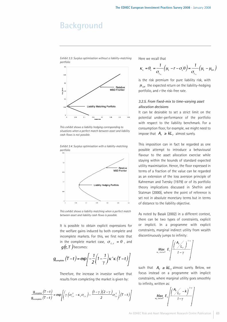
69An EDHEC Risk and Asset Management Research Centre Publication
The EDHEC European Investment Practices Survey 2008 - January 2008
Exhibit 3.3: Surplus optimisation without a liability-matching portfolio
This exhibit shows a liability hedging corresponding to situations when a perfect match between asset and liability cash flows is not possible.
Exhibit 3.4: Surplus optimisation with a liability-matching portfolio
This exhibit shows a liability matching when a perfect match between asset and liability cash flows is possible.
It is possible to obtain explicit expressions for the welfare gains induced by both complete and incomplete markets. For this, we first note that in the complete market case, 0, =εσ L , and
( )Ttg , becomes:
Therefore, the increase in investor welfare that results from completing the market is given by:
Here we recall that
κL = θL =
1σL ,ε
μL - r - σL'θ( ) =
1σL ,ε
μL - μLH( )
is the risk premium for pure liability risk, with
LHμ the expected return on the liability-hedging portfolio, and r the risk-free rate.
3.2.5. From fixed-mix to time-varying asset allocation decisionsIt can be desirable to set a strict limit on the potential under-performance of the portfolio with respect to the liability benchmark. For a consumption floor, for example, we might need to impose that TT kLA ≥ almost surely.
This imposition can in fact be regarded as one possible attempt to introduce a behavioural flavour to the asset allocation exercise while staying within the bounds of standard expected utility maximisation. Hence, the floor expressed in terms of a fraction of the value can be regarded as an extension of the loss aversion principle of Kahneman and Tversky (1979) or of its portfolio theory implications discussed in Shefrin and Statman (2000), where the point of reference is set not in absolute monetary terms but in terms of distance to the liability objective.
As noted by Basak (2002) in a different context, there can be two types of constraints, explicit or implicit. In a programme with explicit constraints, marginal indirect utility from wealth discontinuously jumps to infinity:
⎥⎥⎥⎥
⎦
⎤
⎢⎢⎢⎢
⎣
⎡
-
⎟⎠⎞
⎜⎝⎛
-
≤≤ γ
γ
1
1
,
T
T
tTstw
LA
EMaxs
such that TT kLA ≥ almost surely. Below, we focus instead on a programme with implicit constraints, where marginal utility goes smoothly to infinity, written as:
⎥⎥⎥⎥
⎦
⎤
⎢⎢⎢⎢
⎣
⎡
-
⎟⎠⎞⎜
⎝⎛ -
-
≤≤ γ
γ
1
1
,
kLA
EMax T
T
tTstws
Background
gcomplete T -t( ) = exp -
12
1-1γ
⎛
⎝⎜⎞
⎠⎟κ ' κ T -t( )
⎡
⎣⎢
⎤
⎦⎥
gcomplete T - t( )gincomplete T - t( )
= exp γ σL ,ε2 - κ Lσ L ,ε( ) -
1 - γ( ) 2 - γ( )2
σ L ,ε2
⎛
⎝⎜⎞
⎠⎟T - t( )
⎡
⎣⎢⎢
⎤
⎦⎥⎥
70 An EDHEC Risk and Asset Management Research Centre Publication
The EDHEC European Investment Practices Survey 2008 - January 2008
The following theorem provides the solution to this constrained optimisation problem in the complete market case. In incomplete markets, the presence of a non-hedgeable source of risk will make it impossible for the (implicit) constraint to hold almost surely.
Theorem 2In the complete market case, the optimal terminal funding ratio obtained as a solution to the programme:
Maxws ,t ≤s ≤T
Et
AT
LT
- k⎛
⎝⎜⎞
⎠⎟
1-γ
1- γ
⎡
⎣
⎢⎢⎢⎢⎢
⎤
⎦
⎥⎥⎥⎥⎥
such that: t
t
T
TQt L
ALA
E L =⎥⎦
⎤⎢⎣
⎡,
where ( )tA is financed by a feasible trading strategy with initial investment ( )0A , is given by:
while the indirect utility function reads:
and the optimal portfolio strategy is:
For a given value of the risk-aversion parameter, the investment in the log-optimal portfolio is lower than in the absence of liability constraints since
11 <⎟⎟⎠
⎞⎜⎜⎝
⎛-
tF
k
and it decreases as the funding ratio decreases towards the threshold level.
The fraction of wealth allocated to the optimal growth portfolio
( ) ( )( ) ( )11'
1rr
wm-
-=
-
-
μσσ
μσσ1
1
'
'
is given by:
Therefore, if we define the floor as tkL , i.e., the value of the liabilities that is consistent with the constraint, and the cushion as kLAt - ,we obtain investment in the growth optimal portfolio that is always equal to a constant multiple m of the difference between the asset value and the floor. That constant coefficient is:
( ) ( )γ
μσσ 11' rm
-=
-1'
It should be noted that this is strongly reminiscent of CPPI (constant proportion portfolio insurance) strategies, which the present setup extends to a relative risk management context.18 While CPPI strategies are designed to prevent terminal wealth from falling below a specific threshold, they are not designed to prevent asset value from falling below a pre-specified fraction of some benchmark value. To the best of our knowledge this result is novel and rationalises the so-called contingent optimisation technique, a concept introduced by Leibowitz and Weinberger (1982, 1983) with no theoretical justification, which it further extends to the relative risk context.19
On the other hand, it should be noted that the fraction of wealth allocated to the liability-hedging portfolio
( )( ) L
LLw
σσ
σσ1
1
'
'-
-
=1'
is given by
( )( )
( )⎟⎟⎠
⎞⎜⎜⎝
⎛--
-
-
tttL
L kLAAγσσ
σσ 1
'
'1
1
1
Background
18 - CPPI strategies were originally introduced by Black and Jones (1987) and Black and Perold (1992).19 - See also Amenc et al. (2004) for the benefits of dynamic asset allocation strategies in the context of the management of downside risk relative to a benchmark.
FT
* = Ft Et ξ t ,T( )( )1-1
γ + kξ t ,T( )⎛
⎝⎜⎞
⎠⎟⎡
⎣⎢
⎤
⎦⎥
-1
ξ t ,T( )( ) -1
γ + k
Jt =1
1- γFt Et ξ t ,T( )( )1-
1
γ + kξ t ,T( )⎛
⎝⎜⎞
⎠⎟⎡
⎣⎢
⎤
⎦⎥
-1
ξ t ,T( )( ) -1
γ + k⎛
⎝⎜⎜
⎞
⎠⎟⎟
1-γ
w * =1
γ1 -
k
Fs
⎛
⎝⎜⎞
⎠⎟σσ '( ) -1
μ - r1( ) + 1 -1
γ1 -
k
Fs
⎛
⎝⎜⎞
⎠⎟⎛
⎝⎜
⎞
⎠⎟ σ '( ) -1
σ L
1' σσ '( ) -1μ - r1( )
γAt -
At kFt
⎛
⎝⎜⎞
⎠⎟=
1' σσ '( ) -1μ - r1( )
γAt - kLt( )
1' σσ '( ) -1μ - r1( )
γAt -
At kFt
⎛
⎝⎜⎞
⎠⎟=
1' σσ '( ) -1μ - r1( )
γAt - kLt( )

71An EDHEC Risk and Asset Management Research Centre Publication
The EDHEC European Investment Practices Survey 2008 - January 2008
The investment in the liability-hedging portfolio is always equal to a constant multiple m’ of the difference between the asset value and the cushion divided by the coefficient of risk-aversion. The multiplier coefficient is
( )( ) L
Lmσσ
σσ1
1
'
''
-
-
=1
It is remarkable that the optimal solutions to a formal ALM problem such as the one presented above are strongly reminiscent of the so-called LDI solutions, which advocate an approach to ALM that is expressed in terms of allocation to three building blocks (cash, liability-matching portfolios, and performance portfolios), as opposed to allocation to standard asset classes, as previously done in the context of surplus optimisation techniques.
This is an approach that has rapidly elicited interest from pension funds, insurance companies, and investment consultants alike. Although they may vary significantly from one provider to another, LDI techniques typically involve a hedge of the duration and convexity risks through several standard building blocks, while keeping some assets free for investing in higher yielding asset classes. These solutions may or may not involve leverage, depending on the institutional investor’s risk aversion. When no leverage is used, a fraction of the assets (known as the liability-matching portfolio) is allocated to risk management, while another fraction is allocated to performance generation. One may actually view LDI as a combination of two strategies, involving investing in immunisation strategies (for risk management) as well as investing in standard asset management solutions (for performance generation). This approach stands in sharp contrast to more traditional surplus optimisation methods, where both objectives (liability risk management and performance generation) are pursued simultaneously in an attempt to achieve the portfolio with the highest possible relative risk/relative return ratio.
Note also that, as outlined in the previous sections, several investment banks have suggested using customised derivatives to perform liability matching, and use leverage so that the full amount of the asset portfolio is still invested in a risky asset. This strategy corresponds to -100% in cash, 100% in a liability-hedging portfolio, and 100% in a market portfolio, which can be rationalised under a specific choice of the risk aversion coefficient. More risk-averse investors, on the other hand, will prefer techniques involving little or no leverage.
In closing, it should be noted that ALM models such as the one introduced above focus on long-horizon asset allocation problems. The case can certainly be made that the long-horizon focus is precisely what is specific to institutional asset allocation decisions, so that it should be regarded as a desirable feature of the model. But regulatory constraints lead to a dramatic shortening of the horizon. In other words, it may well be the case that the optimal solution from a long-horizon standpoint violates some short-term constraints. This situation might lead to the adoption of sub-optimal policies from a long-term ALM perspective.
3.3. Implementing Liability-Hedging PortfoliosThe usefulness and limitations of these ALM techniques, and the question of how to design the liability-hedging or liability-matching portfolio, can perhaps be best understood through numerical examples. While cash instruments such as bonds can be used in the design of liability-matching portfolios, derivative instruments such as futures and swaps typically allow a more efficient implementation of the strategy.
Broadly, there are two main risks factors in the real-world liability portfolios of insurance companies: interest rate risk and inflation risk (see below for more details on the relative importance of these two risk factors). We will
Background

72 An EDHEC Risk and Asset Management Research Centre Publication
The EDHEC European Investment Practices Survey 2008 - January 2008
review the financial instruments (cash and derivative instruments) that can be involved in the design of liability-matching portfolios. The illustrations below will focus either on protection with respect to inflation risk or on protection with respect to interest rate risk, depending on the example at hand.
Overall, we will argue that, while cash instruments such as bonds can be used in the design of liability-matching portfolios, derivative instruments such as futures and swaps typically allow more efficient replication of the interest rate risk (and, if necessary of the inflation risk) present in liability structures.
Background
Comparison contingent optimisation technique vs. dynamic LDI
This part will elaborate on dynamic allocation methods in an ALM context. Several methods based on portfolio insurance techniques in a relative return context are examined. We will shed light on contingent immunisation (Leibowitz and Weinberger 1982, 1983) and the dynamic LDI approach (which is a specific application of the dynamic core satellite approach of Amenc, Malaise, and Martellini (2004) to an ALM context where the core portfolio is linked to the liabilities).
Contingent immunisation is a method for bond portfolio managers to practise active portfolio management, to a certain extent, while protecting themselves from losses beyond a predetermined level of minimal acceptable returns (safety-net). To guarantee the safety-net level of returns the manager is required to start immunising the portfolio once the “trigger yield” is reached.
In the dynamic LDI approach the fractions invested in both the liability-oriented benchmark and performance-generating portfolio portfolios are dynamically adjusted. Rebalancing at certain times will modify the portfolio tracking error. In this way, there is room for active portfolio management if the performance-generating portfolio outperforms the liability-oriented benchmark, and there is protection from major under-performance of the benchmark if things turn out to be the other way around. In the dynamic LDI approach the floor is defined in terms of the liability-oriented benchmark. Consequently, the dynamic LDI approach concentrates on relative returns, whereas its predecessor, the CPPI, focuses on absolute returns. This dynamic LDI approach can also be used in strategies other than those for pure asset-liability management.
It is obvious that both contingent immunisation and the dynamic LDI approach are dynamic. Furthermore, both strategies impose minimum acceptable returns. In contingent immunisation this floor is a certain number of basis points below current market returns. For the dynamic LDI approach the floor is expressed in terms of the liability-oriented benchmark benchmark.
In addition, the aim of both methods is to avoid extreme negative returns while maintaining upside potential. Asymmetric return distributions are the result. In comparison with the distribution of active managers, the downside risk is limited; the left tail is truncated. In general, the right tail is less fat for both dynamic allocation methods; there is a little less upside potential.
For both methods, rebalancing occurs at discrete time intervals so there is a tiny risk, in the case of extreme events, of the portfolio value’s falling beneath the floor. Historical evidence, however, suggests that such events are highly unlikely.
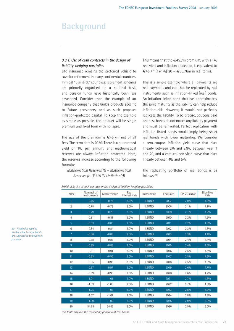
73An EDHEC Risk and Asset Management Research Centre Publication
The EDHEC European Investment Practices Survey 2008 - January 2008
3.3.1. Use of cash contracts in the design of liability-hedging portfoliosLife insurance remains the preferred vehicle to save for retirement in many continental countries. In most “Bismarck” countries, retirement schemes are primarily organised on a national basis and pension funds have historically been less developed. Consider then the example of an insurance company that builds products specific to future pensioners, and as such proposes inflation-protected capital. To keep the example as simple as possible, the product will be single premium and fixed term with no lapse.
The size of the premium is €45.7m net of all fees. The term date is 2026. There is a guaranteed yield of 1% per annum, and mathematical reserves are always inflation protected. Here, the reserves increase according to the following formula:
Mathematical Reserves (t) = Mathematical Reserves (t-1)*1.01*(1+inflation(t))
This means that the €45.7m premium, with a 1% real yield and inflation protected, is equivalent to €45.7 * (1+1%)^20 = €55.76m in real terms.
This is a simple example where all payments are real payments and can thus be replicated by real instruments, such as inflation-linked [real] bonds. An inflation-linked bond that has approximately the same maturity as the liability can help reduce inflation risk. However, it would not perfectly replicate the liability. To be precise, coupons paid on these bonds do not match any liability payment and must be reinvested. Perfect replication with inflation-linked bonds would imply being short real bonds with lower maturities. We consider a zero-coupon inflation yield curve that rises linearly between 2% and 2.9% between year 1 and 20, and a zero-coupon yield curve that rises linearly between 4% and 5%.
The replicating portfolio of real bonds is as follows:20
Background
20 - Nominal is equal to market value because bonds are supposed to be bought at par value.
Index Nominal of instruments Market Value Real
Interest Rate Instrument End Date CPI ZC curve Risk-Free Rate
1 -0.76 -0.76 2.0% ILBOND 2007 2.0% 4.0%
2 -0.78 -0.78 2.0% ILBOND 2008 2.1% 4.1%
3 -0.79 -0.79 2.0% ILBOND 2009 2.1% 4.2%
4 -0.81 -0.81 2.0% ILBOND 2010 2.2% 4.2%
5 -0.83 -0.83 2.0% ILBOND 2011 2.2% 4.3%
6 -0.84 -0.84 2.0% ILBOND 2012 2.3% 4.3%
7 -0.86 -0.86 2.0% ILBOND 2013 2.3% 4.4%
8 -0.88 -0.88 2.0% ILBOND 2014 2.4% 4.4%
9 -0.89 -0.89 2.0% ILBOND 2015 2.4% 4.5%
10 -0.91 -0.91 2.0% ILBOND 2016 2.5% 4.5%
11 -0.93 -0.93 2.0% ILBOND 2017 2.5% 4.6%
12 -0.95 -0.95 2.0% ILBOND 2018 2.5% 4.6%
13 -0.97 -0.97 2.0% ILBOND 2019 2.6% 4.7%
14 -0.99 -0.99 2.0% ILBOND 2020 2.6% 4.7%
15 -1.01 -1.01 2.0% ILBOND 2021 2.7% 4.8%
16 -1.03 -1.03 2.0% ILBOND 2022 2.7% 4.8%
17 -1.05 -1.05 2.0% ILBOND 2023 2.8% 4.9%
18 -1.07 -1.07 2.0% ILBOND 2024 2.8% 4.9%
19 -1.09 -1.09 2.0% ILBOND 2025 2.9% 5.0%
20 54.65 54.65 2.0% ILBOND 2026 2.9% 5.0%
Exhibit 3.5: Use of cash contacts in the design of liability-hedging portfolios
This table displays the replicating portfolio of real bonds.

74 An EDHEC Risk and Asset Management Research Centre Publication
The EDHEC European Investment Practices Survey 2008 - January 2008
In this case, the portfolio is worth €37m and €54m needs to be invested in a 20-year real bond. Perfect replication of the liability is never possible because of the lack of available maturities in the inflation-linked market. In addition, any portfolio that cannot be short bonds would be significantly different from the replicating portfolio and thus have greater risk.
This situation calls for the use of derivatives, as will be shown in sub-section 3.3.4. In this case, zero-coupon inflation swaps would be the unit bricks of the replication portfolio.
In practice, the bulk of the portfolio could be made up of real bonds, as derivatives are used mainly as an adjustment. In our example, the present value of the liability, €37.23m, can be invested in the designated real bond, with zero-coupon inflation swaps to adjust the portfolio. It is worth mentioning here that, depending on the structure of the portfolio inflation, swaps may be needed in larger amounts than inflation bonds where static replication is desired. See section 3.3.4 for a description of the use of swaps in the design of replicating portfolios.
3.3.2. Use of futures contracts in the design of liability-hedging portfoliosIn the next section, we will argue that swaps contracts are convenient tools for proper management of the assets and liabilities mismatch. On the other hand, insurance companies wishing to focus on exchange-traded derivatives, as opposed to OTC derivatives, may prefer to use futures contracts in the context of a simple duration-matching strategy. We describe below a simple exercise illustrating the use of futures contracts for interest rate management in an ALM perspective.21 Goltz, Martellini, and Ziemann (2006), to which we refer the reader, are the source of this illustration.
Mismatches between the duration of assets and that of liabilities can expose insurance companies to significant interest rate risk. This exposure may
represent a large, unacknowledged, strategic bet on interest rates and the mismatch in duration exposes the company to uncompensated risk. Assuming, for example, a liability structure that leads to an average duration of between 10 and 15 years, it is obvious that using government bonds of a duration significantly lower than that of the liabilities will result in opportunity costs and startling risk/reward differences.
It should be noted at this point that it is not unusual for insurance companies to have liability streams of long duration. In Belgium, for instance, there are single and regular premium products with a fixed term that corresponds to the retirement age. When policyholders are under 40, the duration of the contracts is greater than twenty years, and overall these contracts may have a substantial duration. As the market for very long-term bonds is underdeveloped, some companies build a risk position that consists of funding a long-term equity book with very long liabilities. These companies have a negative duration gap; in other words, they have a net short position in very long-term fixed cash flows.22
A drop in interest rates will have a greater impact on the value of the liabilities than on the value of the assets, resulting in a sharp decrease in the size of the surplus. A positive duration gap indicates, on average, that assets are more interest rate sensitive than liabilities. Thus, when interest rates rise (fall), assets will fall proportionately more (less) in value than will liabilities and the market value of equity will fall (rise) accordingly. On the other hand, a negative duration gap indicates that weighted liabilities are more interest rate sensitive than assets. Thus, when interest rates rise (fall), assets will fall proportionately less (more) in value than will liabilities and the market value of equity will rise (fall).
On the liability side, in an attempt to focus on a stylised liability structure, we model the
Background
21 - Investors can also use repo transactions to adjust the duration of a bond portfolio, as outlined below.22 - It must be underlined that duration is but a first-order approximation of the measure of exposure with respect to small and parallel changes in the yield curve. When large changes in the level and/or changes in the shape of the yield curve are to be expected, other risk indicators such as convexity or factor-dura-tion (slope-duration, and curvature-duration) can be used (Martellini, Priaulet, and Priaulet 2003).

75An EDHEC Risk and Asset Management Research Centre Publication
The EDHEC European Investment Practices Survey 2008 - January 2008
liabilities as a short position in a global bond index, which can be represented by a zero-coupon bond with constant time-to-maturity. A standard interest rate model (Longstaff and Schwartz 1992) allows us to easily price liabilities modelled in this manner. Our chosen method of representing liabilities reflects the primacy of changes in interest rates and changes in interest rate volatility among the factors that affect an insurance company’s liabilities. As a result, liabilities would be perfectly correlated with returns on a bond index. In practice, there are certainly other factors, such as actuarial uncertainty, that determine the returns on liabilities. It is for this reason that we introduce a disturbance term in our liability process as a convenient reduced-form way to achieve a target correlation between liabilities and the discount bond (see Goltz, Martellini, and Ziemann 2006).
We assume that the liability duration is equal to 10 years, and consider the effect of investing in different derivatives strategies on the performance relative to liabilities. To isolate the effects of short-term changes in the interest rate and interest rate volatility, we assess the gap between assets and liabilities at a three-month horizon.
We look first at our base case, where the investor holds a position in a standard average maturity contract, i.e., the Bund futures contract. Assuming initial full funding, we use shortfall measures to assess the outcome of investing 100% of the assets in this strategy. Since the duration of the Bund future is lower than that of the liabilities we model, the shortfall risk is expected to be significant. As highlighted above, it is critical for institutional investors to have long-term maturity instruments for hedging purposes, as the convexity of the price-yield relation increases for bonds with longer maturities. The significant shortfall risk for the two Bund futures strategies actually stems from the greater duration of the liabilities. This problem is all the more significant in times of low interest rate coupons, which
also have a positive impact on convexity. We therefore assess the usefulness of a 30-year bond future for hedging purposes. The duration of this contract is roughly 18 years, which is actually higher than the duration for the liabilities in our model (10 years), while the duration of the Bund contract is lower in both cases. To ensure proper risk management, we obtain the weights of the Bund and Buxl strategy by minimising the shortfall variance.23
The figure on the following page shows the distribution of the difference between assets and liabilities at the three-month horizon. Again, this figure allows us to assess the impact of interest rate shocks on the investor’s situation, given that he/she faces liability constraints. The histograms on the left show the surplus/deficit distribution when the liabilities correspond exactly to a short position in a bond index. The histograms on the right show the surplus/deficit distribution when the liabilities have a correlation of only 0.8 with the bond index—that is, when we introduce a white noise disturbance. The upper graphs correspond to a holding of the simple Bund futures strategy, the middle graphs to the Buxl futures strategy, and the lower graphs to attempts to match the duration of liabilities by mixing both strategies. It is clear that the Buxl futures strategy leads to a lower variability of the distribution, while the duration-matching strategy achieves the lowest distribution. In addition, it appears that even if the liabilities deviate significantly from a zero-coupon bond the duration-matching technique is useful, i.e., the main risk stems from the interest rate changes.
Background
23 - We favour this approach to simple duration calculations, which rely on certain assumptions, notably that the yield curve is affected only by small parallel shifts, which may not hold in a general setup.
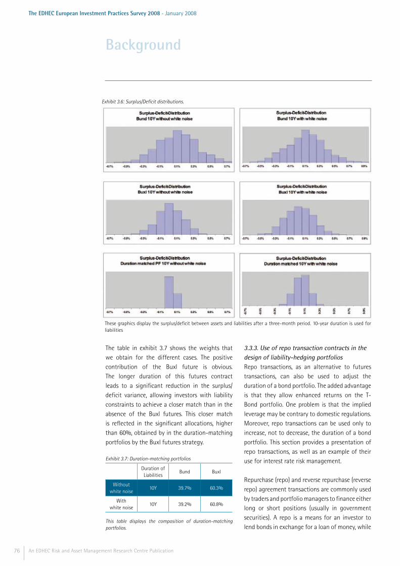
76 An EDHEC Risk and Asset Management Research Centre Publication
The EDHEC European Investment Practices Survey 2008 - January 2008
The table in exhibit 3.7 shows the weights that we obtain for the different cases. The positive contribution of the Buxl future is obvious. The longer duration of this futures contract leads to a significant reduction in the surplus/deficit variance, allowing investors with liability constraints to achieve a closer match than in the absence of the Buxl futures. This closer match is reflected in the significant allocations, higher than 60%, obtained by in the duration-matching portfolios by the Buxl futures strategy. Exhibit 3.7: Duration-matching portfolios
Duration of Liabilities
Bund Buxl
Without white noise
10Y 39.7% 60.3%
With white noise
10Y 39.2% 60.8%
This table displays the composition of duration-matching portfolios.
3.3.3. Use of repo transaction contracts in the design of liability-hedging portfoliosRepo transactions, as an alternative to futures transactions, can also be used to adjust the duration of a bond portfolio. The added advantage is that they allow enhanced returns on the T-Bond portfolio. One problem is that the implied leverage may be contrary to domestic regulations. Moreover, repo transactions can be used only to increase, not to decrease, the duration of a bond portfolio. This section provides a presentation of repo transactions, as well as an example of their use for interest rate risk management.
Repurchase (repo) and reverse repurchase (reverse repo) agreement transactions are commonly used by traders and portfolio managers to finance either long or short positions (usually in government securities). A repo is a means for an investor to lend bonds in exchange for a loan of money, while
Background
Exhibit 3.6: Surplus/Deficit distributions.
These graphics display the surplus/deficit between assets and liabilities after a three-month period. 10-year duration is used for liabilities

77An EDHEC Risk and Asset Management Research Centre Publication
The EDHEC European Investment Practices Survey 2008 - January 2008
a reverse repo is a means for an investor to lend money in exchange for a loan of securities. More precisely, a repo agreement is a commitment by the seller of a security to buy it back from the buyer at a specified price and at a given future date. It can be viewed as a collateralised loan, the collateral here being the security. A reverse repo agreement is the same transaction viewed from the buyer's perspective. The repo desk acts as the intermediary between the investors who want to borrow cash and lend securities and the investors who want to lend cash and borrow securities. The borrower of cash will pay the bid repo rate times the amount of cash borrowed while the lender of cash will get the ask repo rate times the amount of cash lent. The repo desk earns the bid-ask spread on all the transactions it brokers. Suppose, for example, that an investor lends EUR1m of the 10-year Bund benchmark bond (the Bund 5% 07/04/2011 with a quoted price of 104.11, on 10/29/2001) over 1 month at a repo rate of 4%. There is 160 days' accrued interest as of the starting date of the transaction. At the beginning of the transaction, the investor will receive an amount of cash equal to the gross price of the bond times the nominal of the loan:
(104.11+5×117/360)%×1,000,000 = €1,057,350
At the end of the transaction, in order to repurchase the securities he will pay the amount of cash borrowed plus the repo interest due over the period:
1,057,350×(1+4%×30/360) = €1,060,875
Repo operations are a way of raising additional cash in a portfolio, allowing the completion of the existing asset profile with new investments that will help reach a targeted structure. This solution is efficient in particular when the government bonds put in repos cannot be sold because the sale will have an undesired accounting impact or because the bonds themselves contribute to the targeted structure in terms of duration, cash flow scheme, or earnings.
Some concrete examples using repos follow:• Objective: to lengthen the duration when no cash is available. If the bonds available in the market are not long enough to reach the duration target, a second layer can be built with the help of repos. Using swaps to lengthen duration may be one solution. Using repos, whose advantages are simplicity and the addition of the repo spread to the revenues, with no need to provide efficiency tests, is an alternative. The disadvantages include less flexibility on maturities selection.
• Objective: to decrease convexity while keeping duration unchanged. This may be achieved by a combination of (1) the sell of a long-dated swap (i.e., fixed payer) and (2) repos as part of the bond portfolio with reinvestment of cash in intermediate maturities. Again, this is an alternative to a full swaps solution.
• Objective: to be long both duration and credit (extension of the first example). The targeted structure may necessitate a volume of assets bigger than the balance sheet size, i.e., there may not be enough room for both government bonds (duration target) and corporate bonds (revenue target and/or liquidity target). Repos may once again be an alternative to swaps. Some documentation may be required to prove that the balance sheet is not at risk with leveraging. It makes sense to argue the following:(1) Government bonds present (almost) no credit risk but duration (AAA rating is better for this purpose).
(2) A credit exposure is achievable without duration (short-term instruments + credit derivatives swap or duration-hedged corporate bonds portfolio).
These two assets are orthogonal regarding duration and credit: there is no leverage here but as a result a synthetic credit bond with duration. Another way to put it is to say that repos’ short-term debt plus reinvestment in credit with hedged duration form a credit return in excess of that on government bonds.
Background

78 An EDHEC Risk and Asset Management Research Centre Publication
The EDHEC European Investment Practices Survey 2008 - January 2008
One should of course also mention the typical use of repo transactions as a way to enhance the performance of a bond portfolio with limited additional risks by earning the repo spread when liquidity is not required of the bonds. In the case of repo bonds that benefit from high demand and for which there are wide spreads below short-term rates, one can reinvest the cash in short-term instruments that may be backed to repo redemption dates. If there is a certain volume of rolled repos, with a minimum amount stable over time, the cash may be pooled and invested in a dedicated mutual fund for horizons longer than those of repo transactions; in AFS, accounting for this investment is with change in fair value in the P&L (no look through). This investment will allow some basis points to be added above the repo spread through more diversification.
3.3.4. Use of swap transactions in the design of liability-hedging portfoliosWe turn below to an illustration of the use of swaps, as opposed to futures contracts, in the design of liability risk management strategies. In a nutshell, interest rate swaps are naturally suitable for cash-flow matching strategies, which involve a perfect static match between the cash flows from the portfolio of assets and the commitments in the liabilities, while exchange-traded futures should be the instruments of choice for immunisation strategies, which allow dynamic management of the residual interest rate risk created by the imperfect match between the assets and liabilities. Moreover, inflation swaps allow the management of both inflation risk and interest rate risk.
We now specifically consider a stylised liability structure for an insurance company that is affected by interest rate risk and inflation risk.
Inflation risk is of particular concern when it comes to non-life insurance contracts. These contracts provide protection against damage to goods and people. Underwriting risk, hedgeable only through reinsurance (and as such considered non-hedgeable), is the largest risk exposure.
However, the present value of the outstanding claims is subject to hedgeable risk factors:• Expected fixed cash flows need to be discounted, which makes for an exposure to interest rates.
• Claims that are settled through judicial schemes and paid late relative to their date of report are usually inflated with legally accrued interest rates. These legal rates are generally revised periodically, which makes for another form of exposure to interest rates.
• Damaged goods must be replaced or repaired for an amount subject to the price of the goods; care and treatment must be provided in the case of bodily injury for an amount subject to the price of health care and services. The sum of exposures to individual components of the consumer price index can be treated statistically as an overall exposure to the consumer price index, which is hedgeable (in particular, as we explain below, by using inflation swaps).
Hence, it appears that all non-life claims are subject to significant inflation exposure. In general, exposure to inflation tends to be much greater in non-life than in life insurance. Life insurance involves primarily the portion of the portfolio linked to pensions, whether they are long-term savings or annuities.
If we consider a liability with benefits that are predominantly inflation-linked, it is clear that inflation-linked assets would be an appropriate match for the liabilities, since the physical assets that give the lowest risk relative to the liabilities are inflation-linked bonds. If the benefits are not linked to inflation, nominal bonds are the asset class that is most correlated with liabilities.
This cash-instrument approach to liability management, however, is not the optimal approach. An alternative asset and liability match would be to buy a risky portfolio of straight bonds or invest in absolute return strategies (a so-called performance-seeking portfolio)
Background

79An EDHEC Risk and Asset Management Research Centre Publication
The EDHEC European Investment Practices Survey 2008 - January 2008
and use the swaps market to convert the bond cash flows into the precise inflation-linked cash flows required to make the projected liability payments. Insurance companies will pay fixed flows (extracted from the portfolio) and receive inflation-linked cash flows tailored to meet the projected liabilities. This technique would provide more precise management of inflation risk than would a technique relying on index-linked gilts.
It would also introduce leverage, and—with potential additional performance from the risky portfolio—result in both a higher expected return and increased risk (the portfolio may under-perform the fixed swap rate).
If liability streams are not inflation-indexed, the hedging strategy involves only interest rate swaps, as illustrated in the figure below.
Background
Exhibit 3.8: Use of inflation and interest swaps for liability-matching portfolios (case of inflation-linked liability streams)
Note that payments are netted so that only the net amount is exchanged between parties.
InvestmentBank
InsuranceCompany
Client
RPI-linked cashflows to matchliability payments
Notional x ((CPPI t+1/CPPI t)-1)
RPI-linkedliability payments
Fixed cash-flows extracted from return on bond portfolio or performance portfolio.
Notional x ((1+fixed rate)T -1)
Exhibit 3.9: Use of interest swaps for liability-matching portfolios (case of non inflation-linked liability streams)
In this case, the hedging strategy only involves interest rate swaps.
Party A Party B
PAY
Fixed Rate %
Floating Rate (Libor)
Fixed
Semi-annually in arrears
Actual/365 basis
Notional amount m
PAYLibor
Fixed semi-annually in advance
Paid semi-annually in advance
Actual/365 basis
Notional amount m
RECEIVE RECEIVE
Payments netted

80 An EDHEC Risk and Asset Management Research Centre Publication
The EDHEC European Investment Practices Survey 2008 - January 2008
Background
Exhibit 3.10: Liability-matching portfolio
This figure shows how to immunise the present value to changes in inflation and interest rates.
Inflation35.61m
2026 Cash Flow34.44m
Non inflated55.76m
@ 2.5%Inflation
@ 5%Interest rate
How to immunise the PV to inflationand interest rate changes…
PV in 2006 (34.44 = (55.76 + 35.61)/((1 + 5%)20)
In an attempt to better illustrate the mechanics of cash-flow matching with derivative instruments, we will reconsider the stylised example in which we used real bonds. A single liability cash-flow equal to €55.76m in real terms is to be paid in 2026. Assuming a 2.5% inflation rate, the expected nominal liability payment amounts to 55.76∙(1+2.5%)20 = €91.37m, i.e., an additional
€35.61m. The present value of these cash-flow payments in 2006 is equal to 34.44 = (55.76+35.61)/((1+5%)20), assuming a 5% discount rate.
The core question in the design of a liability-matching portfolio is how to immunise the present value to changes in inflation and interest rates (see figure below).
Exhibit 3.11: Cash-flow matching strategy for the insurance company
Swap Counterpart
Insurancecompany
Receives (1 + i2006)x (1 + i2007) x… x (1 + i2026)
Pays a single ZC breakeven inflation rate of 2.9%
To achieve perfect inflation and interest rate risk management, the insurance company enters a swap with a nominal of €55.76m, for which it will make a single zero-coupon payment based on a breakeven rate assumed to be 2.9% and will receive €55.76m * Inflation Index (2026)/Inflation Index (2006). This assumption means that the nominal yield on a 20-year bond is 290 bps higher (4.51%) than the real yield on a 20-year inflation-protected bond (1.61%). It also means that inflation would have to average more than 2.9% per year until the maturity of the bond for the inflation-linked bond to do as well as the nominal bond of similar
term. Note that investors do not necessarily expect inflation to be as high as 2.9%. Since they do not know what the future will bring, they are willing to sacrifice some current yield for inflation protection on the principal. In other words, there is an inflation risk premium embedded in this 2.9% rate. In 2026, the insurance company must pay 98.77=55.76∙(1+2.9%)20 million euros. To face this payment, assuming a 4.51% current zero-coupon yield on the 20-year horizon, the insurance company buys 20-year zero-coupon bonds (see exhibit 3.11) for 40.88=98.77/((1+4.51%)20).
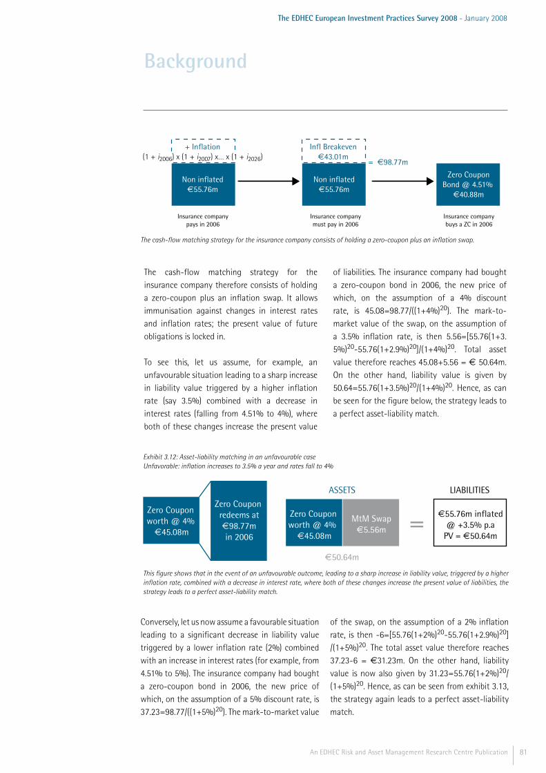
81An EDHEC Risk and Asset Management Research Centre Publication
The EDHEC European Investment Practices Survey 2008 - January 2008
The cash-flow matching strategy for the insurance company therefore consists of holding a zero-coupon plus an inflation swap. It allows immunisation against changes in interest rates and inflation rates; the present value of future obligations is locked in.
To see this, let us assume, for example, an unfavourable situation leading to a sharp increase in liability value triggered by a higher inflation rate (say 3.5%) combined with a decrease in interest rates (falling from 4.51% to 4%), where both of these changes increase the present value
of liabilities. The insurance company had bought a zero-coupon bond in 2006, the new price of which, on the assumption of a 4% discount rate, is 45.08=98.77/((1+4%)20). The mark-to-market value of the swap, on the assumption of a 3.5% inflation rate, is then 5.56=[55.76(1+3.5%)20-55.76(1+2.9%)20]/(1+4%)20. Total asset value therefore reaches 45.08+5.56 = € 50.64m. On the other hand, liability value is given by 50.64=55.76(1+3.5%)20/(1+4%)20. Hence, as can be seen for the figure below, the strategy leads to a perfect asset-liability match.
Background
Non inflated55.76m
Infl Breakeven43.01m
Non inflated55.76m
Zero CouponBond @ 4.51%
40.88m
Insurance companypays in 2006
Insurance companymust pay in 2006
Insurance companybuys a ZC in 2006
= 98.77m
+ Inflation(1 + i2006) x (1 + i2007) x… x (1 + i2026)
The cash-flow matching strategy for the insurance company consists of holding a zero-coupon plus an inflation swap.
Exhibit 3.12: Asset-liability matching in an unfavourable caseUnfavorable: inflation increases to 3.5% a year and rates fall to 4%
This figure shows that in the event of an unfavourable outcome, leading to a sharp increase in liability value, triggered by a higher inflation rate, combined with a decrease in interest rate, where both of these changes increase the present value of liabilities, the strategy leads to a perfect asset-liability match.
Zero Coupon worth @ 4%
45.08m
Zero Coupon worth @ 4%
45.08m
MtM Swap5.56m
Zero Coupon redeems at
98.77min 2006
55.76m inflated@ +3.5% p.a
PV = 50.64m
ASSETS LIABILITIES
50.64m
=
Conversely, let us now assume a favourable situation leading to a significant decrease in liability value triggered by a lower inflation rate (2%) combined with an increase in interest rates (for example, from 4.51% to 5%). The insurance company had bought a zero-coupon bond in 2006, the new price of which, on the assumption of a 5% discount rate, is 37.23=98.77/((1+5%)20). The mark-to-market value
of the swap, on the assumption of a 2% inflation rate, is then -6=[55.76(1+2%)20-55.76(1+2.9%)20]/(1+5%)20. The total asset value therefore reaches 37.23-6 = €31.23m. On the other hand, liability value is now also given by 31.23=55.76(1+2%)20/(1+5%)20. Hence, as can be seen from exhibit 3.13, the strategy again leads to a perfect asset-liability match.
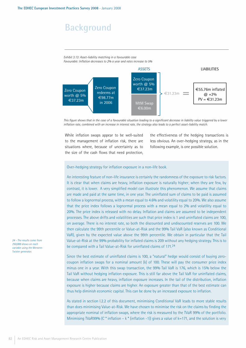
82 An EDHEC Risk and Asset Management Research Centre Publication
The EDHEC European Investment Practices Survey 2008 - January 2008
While inflation swaps appear to be well-suited to the management of inflation risk, there are situations where, because of uncertainty as to the size of the cash flows that need protection,
the effectiveness of the hedging transactions is less obvious. An over-hedging strategy, as in the following example, is one possible solution.
Background
24 - The results come from 250,000 draws on each variable using the Mersene-Twister generator.
Over-hedging strategy for inflation exposure in a non-life book.
An interesting feature of non-life insurance is certainly the randomness of the exposure to risk factors. It is clear that when claims are heavy, inflation exposure is naturally higher; when they are few, by contrast, it is lower. A very simplified model can illustrate this phenomenon. We assume that claims are made and paid at the same time, in one year. The uninflated sum of claims to be paid is assumed to follow a lognormal process, with a mean equal to 4.6% and volatility equal to 20%. We also assume that the price index follows a lognormal process with a mean equal to 2% and volatility equal to 20%. The price index is released with no delay. Inflation and claims are assumed to be independent processes. The above drifts and volatilities are such that price index is 1 and uninflated claims are 100, on average. There is no interest rate, so both the discounted and undiscounted reserves are 100. We then calculate the 99th percentile or Value-at-Risk and the 99% Tail VaR (also known as Conditional VaR), given by the expected value above the 99th percentile. We obtain in particular that the Tail Value-at-Risk at the 99% probability for inflated claims is 209 without any hedging strategy. This is to be compared with a Tail Value-at-Risk for uninflated claims of 171.24
Since the best estimate of uninflated claims is 100, a “natural” hedge would consist of buying zero-coupon inflation swaps for a nominal amount (k) of 100. These will pay the consumer price index minus one in a year. With this swap transaction, the 99% Tail VaR is 176, which is 15% below the Tail VaR without hedging inflation exposure. This is still far above the Tail VaR for uninflated claims, because when claims are heavy, inflation exposure increases. In the tail of the distribution, inflation exposure is higher because claims are higher. An exposure greater than that of the best estimate can thus help diminish economic capital. This can be done by an increased exposure to inflation.
As stated in section I.2.2 of this document, minimising Conditional VaR leads to more stable results than does minimising Value-at-Risk. We have chosen to minimise the risk on the claims by finding the appropriate nominal of inflation swaps, where the risk is measured by the TVaR 99% of the portfolio.Minimising TVaR99% (C * inflation – k * (inflation -1)) gives a value of k=171, and the solution is very
Exhibit 3.13: Asset-liability matching in a favourable caseFavourable: Inflation decreases to 2% a year and rates increase to 5%
This figure shows that in the case of a favourable situation leading to a significant decrease in liability value triggered by a lower inflation rate, combined with an increase in interest rate, the strategy also leads to a perfect asset-liability match.
Zero Coupon worth @ 5%
37.23m
Zero Coupon worth @ 5%
37.23m
MtM Swap6.00m
Zero Coupon redeems at
98.77min 2006
55.76m inflated@ +2%
PV = 31.23m31.23m
ASSETS LIABILITIES
=
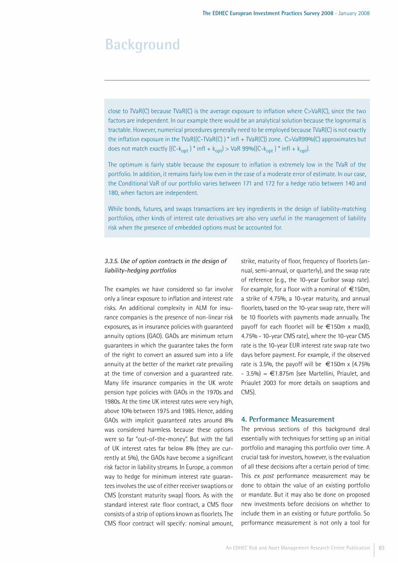
83An EDHEC Risk and Asset Management Research Centre Publication
The EDHEC European Investment Practices Survey 2008 - January 2008
Background
3.3.5. Use of option contracts in the design of liability-hedging portfolios
The examples we have considered so far involve only a linear exposure to inflation and interest rate risks. An additional complexity in ALM for insu-rance companies is the presence of non-linear risk exposures, as in insurance policies with guaranteed annuity options (GAO). GAOs are minimum return guarantees in which the guarantee takes the form of the right to convert an assured sum into a life annuity at the better of the market rate prevailing at the time of conversion and a guaranteed rate. Many life insurance companies in the UK wrote pension type policies with GAOs in the 1970s and 1980s. At the time UK interest rates were very high, above 10% between 1975 and 1985. Hence, adding GAOs with implicit guaranteed rates around 8% was considered harmless because these options were so far “out-of-the-money”. But with the fall of UK interest rates far below 8% (they are cur-rently at 5%), the GAOs have become a significant risk factor in liability streams. In Europe, a common way to hedge for minimum interest rate guaran-tees involves the use of either receiver swaptions or CMS (constant maturity swap) floors. As with the standard interest rate floor contract, a CMS floor consists of a strip of options known as floorlets. The CMS floor contract will specify: nominal amount,
strike, maturity of floor, frequency of floorlets (an-nual, semi-annual, or quarterly), and the swap rate of reference (e.g., the 10-year Euribor swap rate). For example, for a floor with a nominal of €150m, a strike of 4.75%, a 10-year maturity, and annual floorlets, based on the 10-year swap rate, there will be 10 floorlets with payments made annually. The payoff for each floorlet will be €150m x max(0, 4.75% - 10-year CMS rate), where the 10-year CMS rate is the 10-year EUR interest rate swap rate two days before payment. For example, if the observed rate is 3.5%, the payoff will be €150m x (4.75% - 3.5%) = €1.875m (see Martellini, Priaulet, and Priaulet 2003 for more details on swaptions and CMS).
4. Performance Measurement The previous sections of this background deal essentially with techniques for setting up an initial portfolio and managing this portfolio over time. A crucial task for investors, however, is the evaluation of all these decisions after a certain period of time. This ex post performance measurement may be done to obtain the value of an existing portfolio or mandate. But it may also be done on proposed new investments before decisions on whether to include them in an existing or future portfolio. So performance measurement is not only a tool for
close to TVaR(C) because TVaR(C) is the average exposure to inflation where C>VaR(C), since the two factors are independent. In our example there would be an analytical solution because the lognormal is tractable. However, numerical procedures generally need to be employed because TVaR(C) is not exactly the inflation exposure in the TVaR((C-TVaR(C) ) * infl + TVaR(C)) zone. C>VaR99%(C) approximates but does not match exactly ((C-kopt ) * infl + kopt) > VaR 99%((C-kopt ) * infl + kopt).
The optimum is fairly stable because the exposure to inflation is extremely low in the TVaR of the portfolio. In addition, it remains fairly low even in the case of a moderate error of estimate. In our case, the Conditional VaR of our portfolio varies between 171 and 172 for a hedge ratio between 140 and 180, when factors are independent.
While bonds, futures, and swaps transactions are key ingredients in the design of liability-matching portfolios, other kinds of interest rate derivatives are also very useful in the management of liability risk when the presence of embedded options must be accounted for.

84 An EDHEC Risk and Asset Management Research Centre Publication
The EDHEC European Investment Practices Survey 2008 - January 2008
Background
monitoring past decisions, but also for determining future investments. In particular, managers of publicly available investment funds generally attach great importance to evaluation of past performance, as past performance often determines future inflows. From an investor’s perspective, it is crucial to understand the meaning and the general scope of each performance measure, as these measures often rely on the validity of specific assumptions. The objective of the current part of the document is to list existing performance measures and to highlight the limitations of each measure. Thus, in the results section, we provide a necessary background for the analysis and interpretation of the measures currently favoured in the industry.
4.1. Performance Evaluation4.1.1. Absolute risk-adjusted performance measuresThese measures evaluate funds’ risk-adjusted returns, without any reference to a benchmark.
4.1.1.1. Sharpe ratio (1966)This ratio, initially called the reward-to-variability ratio, is defined by:
)(
)(
P
FPP R
RRES
σ
-=
where:E RP( ) denotes the expected return of the portfolio;
RF denotes the return on the risk-free asset;σ ( )RP denotes the standard deviation of the portfolio returns.This ratio measures the return of a portfolio in excess of the risk-free rate, also called the risk premium, over the total risk of the portfolio, measured by its standard deviation. It is drawn from the capital market line, and not the Capital Asset Pricing Model (CAPM). It does not refer to a market index and is not therefore subject to Roll's (1977) criticism that the market portfolio is not observable. Since this ratio is based on the total risk of the portfolio, made up of the market risk and the unsystematic risk taken by the manager, it
enables the performance evaluation of relatively undiversified portfolios. It is also suitable for evaluating the performance of a portfolio that represents an individual's total investment.
This ratio has been subject to generalisations since it was initially defined. It thus offers significant possibilities for evaluating portfolio performance, while remaining simple to calculate. One of the most common variations on this measure involves replacing the risk-free asset with a benchmark portfolio. The measure is then called the information ratio (Sharpe 1994) and will be presented in the section below on relative risk-adjusted measures.
4.1.1.2. Treynor ratio (1965)The Treynor ratio is defined by:
P
FPP
RRET
β
-=
)(
where:E RP( ) denotes the expected return of the portfolio;RF denotes the return on the risk-free asset;βP denotes the beta of the portfolio.
This ratio measures the relationship between the return on the portfolio, above the risk-free rate, and its systematic risk. The Treynor ratio is drawn directly from the CAPM. Calculating this indicator—and estimating the beta of the portfolio—requires the choice of a reference index. The results, as Roll’s criticism makes clear, can then depend heavily on that choice. The Treynor ratio is particularly appropriate for a well-diversified portfolio, as it takes only the systematic risk of the portfolio into account—that is, the share of the risk that is impervious to diversification. It is also for this reason that the Treynor ratio is the most appropriate indicator for evaluating the performance of a portfolio that constitutes only a part of the investor's assets.
Since the investor has diversified his investments, the systematic risk of his portfolio is all that matters.
85An EDHEC Risk and Asset Management Research Centre Publication
The EDHEC European Investment Practices Survey 2008 - January 2008
4.1.1.3. Measures based on VaRValue-at-Risk (VaR) enables expression in a single value of the risks associated with a portfolio diversified over several asset classes. VaR measures the risk of a portfolio as the maximum amount of the loss that the portfolio can sustain for a given level of confidence. This definition of risk can be used to calculate a risk-adjusted return indicator of the performance of a portfolio. To define a logical indicator, we divide the VaR by the initial value of the portfolio and thus obtain a percentage loss on the total value of the portfolio. We then calculate a Sharpe-like indicator in which the standard deviation is replaced with the risk indicator based on the VaR as it was defined or:
0P
P
FP
VVaR
RR -
where:
PR denotes the return on the portfolio;
FR denotes the return on the risk-free asset;
PVaR denotes the VaR of the portfolio;0
PV denotes the initial value of the portfolio.
Note that the calculation of VaR presupposes the choice of a confidence threshold. So VaR-based ratios are comparable only for portfolios with identical confidence thresholds. 4.1.2. Relative risk-adjusted performance measuresThese measures evaluate funds’ risk-adjusted returns with respect to a benchmark.4.1.2.1. Jensen’s alpha (1968)Jensen's alpha is the difference between the return on the portfolio in excess of the risk-free rate and the return explained by the market model, or:
))(()( FMPPFP RRERRE -+=- βα
It is calculated by carrying out the following regression:
PtFtMtPPFtPt RRRR εβα +-+=- )(
The Jensen measure is based on the CAPM.
The term ))(( FMP RRE -β measures the return on the portfolio forecast by the model.
Pα measures the share of additional return that can be attributed to the manager's choices.
The statistical significance of alpha can be evaluated by calculating the t-statistic of the regression, which is equal to the estimated value of the alpha divided by its standard deviation. This value is provided with the results of the regression. Assuming that the alpha values are normally distributed, a t-statistic greater than two indicates that the likelihood of having obtained the result through luck, rather than through skill, is necessarily less than 5%. In this case, the average value of alpha is significantly different from zero.
Unlike the Sharpe and Treynor ratios, the Jensen measure contains the benchmark. As with the Treynor ratio, the systematic risk alone is taken into account, but this method, unlike the Sharpe and Treynor ratios, does not allow portfolios with different levels of risk to be compared. The value of alpha is actually proportional to the level of risk taken, as measured by the beta. To compare portfolios with different levels of risk, we can calculate the Black-Treynor ratio:25
P
P
β
α
Jensen’s alpha can be used to rank portfolios within peer groups. Peer groups group portfolios that are managed in a similar manner and therefore have comparable levels of risk.
The Jensen measure is subject to the same criticism as the Treynor measure: the result depends on the choice of reference index. In addition, when managers use a market-timing strategy, which involves varying the beta in accordance with anticipated movements in the market, Jensen’s alpha often becomes negative and does not then reflect the real performance of the manager. Performance analysis models taking beta variations into account have been developed
Background
25 - See Treynor and Black (1973).

86 An EDHEC Risk and Asset Management Research Centre Publication
The EDHEC European Investment Practices Survey 2008 - January 2008
by Treynor and Mazuy and by Henriksson and Merton.
4.1.2.3. Information ratioThe information ratio, which is sometimes called the appraisal ratio, is the residual return of the portfolio over its residual risk. The residual return of a portfolio corresponds to the share of the return that is not explained by the benchmark. It results from the choices made by the manager to overweight securities that he hopes will have a return greater than that of the benchmark. The residual or diversifiable risk measures the residual return variations. It is the tracking error of the portfolio and the standard deviation of the difference in return between the portfolio and its benchmark. The lower its value, the closer the risk of the portfolio to the risk of its benchmark. Sharpe (1994) depicts the information ratio, in which the risk-free asset is replaced by a benchmark portfolio, as a generalisation of his ratio. The relationship below defines the information ratio:
)(
)()(
BP
BP
RR
REREIR
-
-=
σ
where B
R denotes the return on the benchmark portfolio.
Managers seek to maximise the value of the information ratio—that is, to reconcile a high residual return and a low tracking error. This ra-tio allows us to check that the risk taken by the manager, in deviating from the benchmark, is sufficiently rewarded. It also indicates the de-gree to which the manager's information is bet-ter or worse than the public information availa-ble and his ability (or lack thereof) to achieve a performance that is better than that of the average manager. The information ratios of well diversified portfolios and those of relatively un-diversified portfolios are not comparable, as this ratio fails to take systematic portfolio risk into account; the use of this ratio to compare the performances of these two kinds of portfolios is thus inappropriate.
4.1.2.4. M² measure: Modigliani and Modigliani (1997)Modigliani and Modigliani (1997) show that the portfolio and its benchmark must have the same risk to be compared in terms of basis points of risk-adjusted performance. So they propose that the portfolio be leveraged or deleveraged using the risk-free asset. They define the following measure:
FFPP
MP RRRRAP +-= )(
σ
σ
where: P
M
σ
σ is the leverage factor;
Mσ denotes the annualised standard deviation of the market returns;
Pσ denotes the annualised standard deviation of the returns of fund P;
PR denotes the annualised return of fund P;
FR denotes the risk-free rate.
This measure evaluates the annualised risk-adjusted performance (RAP) of a portfolio in relation to the market benchmark, expressed in percentage terms. For Modigliani and Modigliani, this measure is easier to understand than the Sharpe ratio. They recommend using the standard deviation of a broad-based market index, such as the S&P 500, as the benchmark for risk comparison, but other benchmarks could also be used. For a fund with any given risk and return, the Modigliani measure is equivalent to the return the fund would have achieved if it had had the same risk as the market index. The relationship therefore allows us to situate the performance of the fund in relation to that of the market. The most attractive funds are those with the highest RAP.
The Modigliani measure is drawn directly from the capital market line. It can be expressed as the Sharpe ratio times the standard deviation of the benchmark index: the two measures are directly proportional. So the Sharpe ratio and the M2 measure give funds the same rankings.
Background
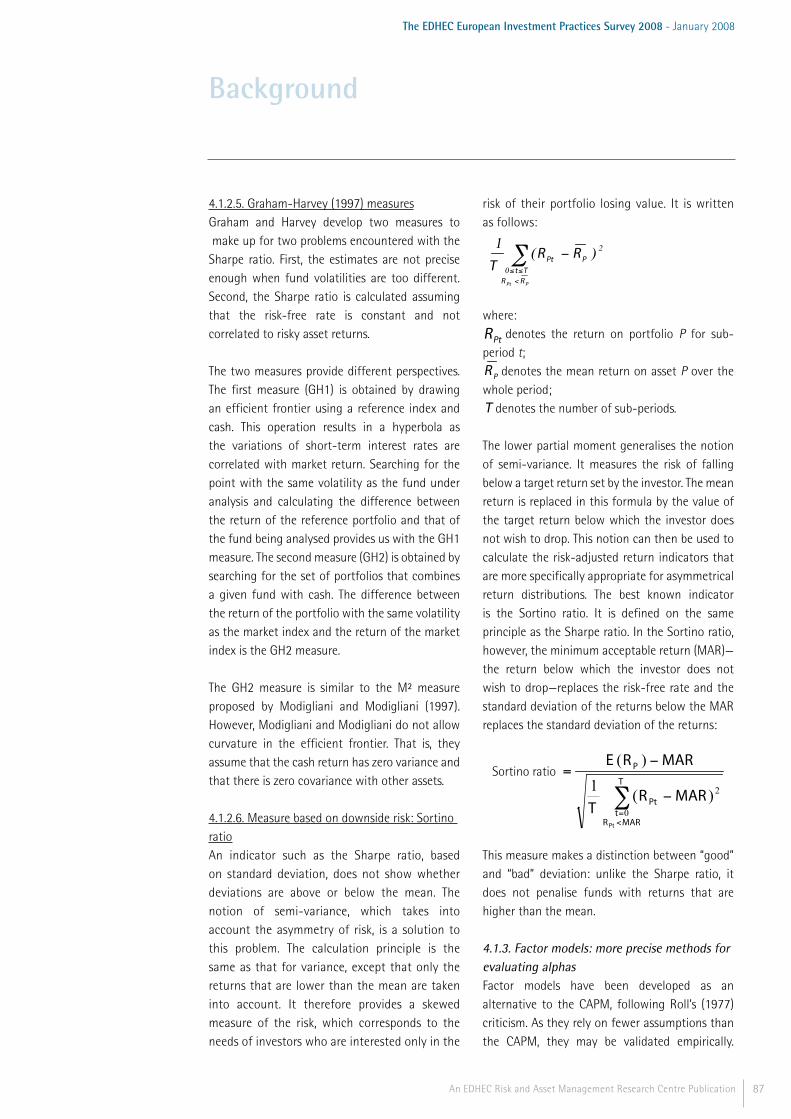
87An EDHEC Risk and Asset Management Research Centre Publication
The EDHEC European Investment Practices Survey 2008 - January 2008
4.1.2.5. Graham-Harvey (1997) measuresGraham and Harvey develop two measures to make up for two problems encountered with the Sharpe ratio. First, the estimates are not precise enough when fund volatilities are too different. Second, the Sharpe ratio is calculated assuming that the risk-free rate is constant and not correlated to risky asset returns.
The two measures provide different perspectives. The first measure (GH1) is obtained by drawing an efficient frontier using a reference index and cash. This operation results in a hyperbola as the variations of short-term interest rates are correlated with market return. Searching for the point with the same volatility as the fund under analysis and calculating the difference between the return of the reference portfolio and that of the fund being analysed provides us with the GH1 measure. The second measure (GH2) is obtained by searching for the set of portfolios that combines a given fund with cash. The difference between the return of the portfolio with the same volatility as the market index and the return of the market index is the GH2 measure.
The GH2 measure is similar to the M² measure proposed by Modigliani and Modigliani (1997). However, Modigliani and Modigliani do not allow curvature in the efficient frontier. That is, they assume that the cash return has zero variance and that there is zero covariance with other assets.
4.1.2.6. Measure based on downside risk: Sortino ratioAn indicator such as the Sharpe ratio, based on standard deviation, does not show whether deviations are above or below the mean. The notion of semi-variance, which takes into account the asymmetry of risk, is a solution to this problem. The calculation principle is the same as that for variance, except that only the returns that are lower than the mean are taken into account. It therefore provides a skewed measure of the risk, which corresponds to the needs of investors who are interested only in the
risk of their portfolio losing value. It is written as follows:
∑<≤≤
-
PPt RRTt
PPt RRT 0
2)(1
where:
PtR denotes the return on portfolio P for sub-period t;
PR denotes the mean return on asset P over the whole period;T denotes the number of sub-periods.
The lower partial moment generalises the notion of semi-variance. It measures the risk of falling below a target return set by the investor. The mean return is replaced in this formula by the value of the target return below which the investor does not wish to drop. This notion can then be used to calculate the risk-adjusted return indicators that are more specifically appropriate for asymmetrical return distributions. The best known indicator is the Sortino ratio. It is defined on the same principle as the Sharpe ratio. In the Sortino ratio, however, the minimum acceptable return (MAR)—the return below which the investor does not wish to drop—replaces the risk-free rate and the standard deviation of the returns below the MAR replaces the standard deviation of the returns:
Sortino ratio
∑<=
-
-=
T
MARRt
Pt
P
Pt
MARRT
MARRE
0
2)(1
)(
This measure makes a distinction between “good” and “bad” deviation: unlike the Sharpe ratio, it does not penalise funds with returns that are higher than the mean.
4.1.3. Factor models: more precise methods for evaluating alphasFactor models have been developed as an alternative to the CAPM, following Roll’s (1977) criticism. As they rely on fewer assumptions than the CAPM, they may be validated empirically.
Background
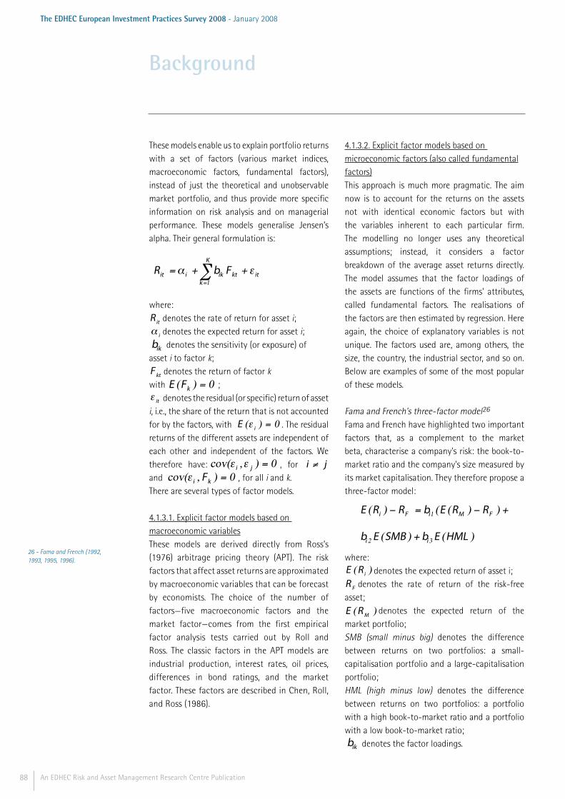
88 An EDHEC Risk and Asset Management Research Centre Publication
The EDHEC European Investment Practices Survey 2008 - January 2008
These models enable us to explain portfolio returns with a set of factors (various market indices, macroeconomic factors, fundamental factors), instead of just the theoretical and unobservable market portfolio, and thus provide more specific information on risk analysis and on managerial performance. These models generalise Jensen’s alpha. Their general formulation is:
∑=
++=K
kitktikiit FbR
1
εα
where:
itR denotes the rate of return for asset i;
iα denotes the expected return for asset i;
ikb denotes the sensitivity (or exposure) of asset i to factor k;
ktF denotes the return of factor k with 0)( =kFE ;
itε denotes the residual (or specific) return of asset i, i.e., the share of the return that is not accounted for by the factors, with 0)( =iE ε . The residual returns of the different assets are independent of each other and independent of the factors. We therefore have: 0),cov( =ji εε , for ji ≠ and 0),cov( =ki Fε , for all i and k.There are several types of factor models.
4.1.3.1. Explicit factor models based on macroeconomic variablesThese models are derived directly from Ross’s (1976) arbitrage pricing theory (APT). The risk factors that affect asset returns are approximated by macroeconomic variables that can be forecast by economists. The choice of the number of factors—five macroeconomic factors and the market factor—comes from the first empirical factor analysis tests carried out by Roll and Ross. The classic factors in the APT models are industrial production, interest rates, oil prices, differences in bond ratings, and the market factor. These factors are described in Chen, Roll, and Ross (1986).
4.1.3.2. Explicit factor models based on microeconomic factors (also called fundamental factors)This approach is much more pragmatic. The aim now is to account for the returns on the assets not with identical economic factors but with the variables inherent to each particular firm. The modelling no longer uses any theoretical assumptions; instead, it considers a factor breakdown of the average asset returns directly. The model assumes that the factor loadings of the assets are functions of the firms' attributes, called fundamental factors. The realisations of the factors are then estimated by regression. Here again, the choice of explanatory variables is not unique. The factors used are, among others, the size, the country, the industrial sector, and so on. Below are examples of some of the most popular of these models.
Fama and French's three-factor model26
Fama and French have highlighted two important factors that, as a complement to the market beta, characterise a company's risk: the book-to-market ratio and the company's size measured by its market capitalisation. They therefore propose a three-factor model:
)()())(()( 321 HMLEbSMBEbRREbRRE iiFMiFi ++-=-
)()())(()( 321 HMLEbSMBEbRREbRRE iiFMiFi ++-=-
where:)( iRE denotes the expected return of asset i;
FR denotes the rate of return of the risk-free asset;
)( MRE denotes the expected return of the market portfolio;SMB (small minus big) denotes the difference between returns on two portfolios: a small-capitalisation portfolio and a large-capitalisation portfolio;HML (high minus low) denotes the difference between returns on two portfolios: a portfolio with a high book-to-market ratio and a portfolio with a low book-to-market ratio;
ikb denotes the factor loadings.
Background
26 - Fama and French (1992, 1993, 1995, 1996).
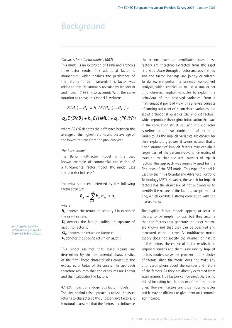
89An EDHEC Risk and Asset Management Research Centre Publication
The EDHEC European Investment Practices Survey 2008 - January 2008
Carhart's four-factor model (1997)This model is an extension of Fama and French's three-factor model. The additional factor is momentum, which enables the persistence of the returns to be measured. This factor was added to take the anomaly revealed by Jegadeesh and Titman (1993) into account. With the same notation as above, this model is written:
)1()()())(()( 4321 YRPRbHMLEbSMBEbRREbRRE iiiFMiFi +++-=-
)1()()())(()( 4321 YRPRbHMLEbSMBEbRREbRRE iiiFMiFi +++-=-
where PR1YR denotes the difference between the average of the highest returns and the average of the lowest returns from the previous year.
The Barra modelThe Barra multifactor model is the best known example of commercial application of a fundamental factor model. The model uses thirteen risk indices.27
The returns are characterised by the following factor structure:
∑=
+=K
kitktiktit ubR
1
α
where:
itR denotes the return on security i in excess of the risk-free rate;
ikb denotes the factor loading or exposure of asset i to factor k;
kα denotes the return on factor k;
iu denotes the specific return on asset i.
This model assumes that asset returns are determined by the fundamental characteristics of the firm. These characteristics constitute the exposures or betas of the assets. The approach therefore assumes that the exposures are known and then calculates the factors.
4.1.3.3. Implicit or endogenous factor modelsThe idea behind this approach is to use the asset returns to characterise the unobservable factors. It is natural to assume that the factors that influence
the returns leave an identifiable trace. These factors are therefore extracted from the asset return database through a factor analysis method and the factor loadings are jointly calculated. To do so, we perform a principal component analysis, which enables us to use a smaller set of unobserved implicit variables to explain the behaviour of the observed variables. From a mathematical point of view, this analysis consists of turning out a set of n correlated variables in a set of orthogonal variables (the implicit factors), which reproduce the original information that was in the correlation structure. Each implicit factor is defined as a linear combination of the initial variables. As the implicit variables are chosen for their explanatory power, it seems natural that a given number of implicit factors may explain a larger part of the variance-covariance matrix of asset returns than the same number of explicit factors. This approach was originally used for the first tests of the APT model. This type of model is used by the firms Quantal and Advanced Portfolio Technology (APT). However, the search for implicit factors has the drawback of not allowing us to identify the nature of the factors, except the first one, which exhibits a strong correlation with the market index.
The explicit factor models appear, at least in theory, to be simpler to use, but they assume that the factors that generate the asset returns are known and that they can be observed and measured without error. As multifactor model theory does not specify the number or nature of the factors, the choice of factor results from empirical studies and there is no unicity. Implicit factors models solve the problem of the choice of factors, since the model does not make any prior assumptions about the number and nature of the factors. As they are directly extracted from asset returns, true factors can be used: there is no risk of including bad factors or of omitting good ones. However, factors are thus mute variables and it may be difficult to give them an economic significance.
Background
27 - A detailed list of the factors used can be found in Amenc and Le Sourd (2003).

90 An EDHEC Risk and Asset Management Research Centre Publication
The EDHEC European Investment Practices Survey 2008 - January 2008
4.1.3.4. Application to performance measureThe multifactor models have a direct application in investment fund performance measurement. By analysing the various dimensions of portfolio risk, it is possible to identify the sources of risk the portfolio is subject to and to evaluate the associated expected reward. The result is better control of portfolio management and an orientation toward better sources of risk, a result that leads to improved performance. These models contribute more information to performance analysis than do the Sharpe, Treynor, and Jensen ratios. The asset returns can be decomposed linearly into several risk factors common to all the assets, but with specific sensitivity to each. Once the model has been determined, we can attribute the contribution of each factor to the overall portfolio performance. This attribution is easily done when the factors are known, as models that use macroeconomic or fundamental factors, but it becomes more difficult when the nature of the factors has not been identified. Performance analysis then consists of evaluating whether the manager is able to orient the portfolio toward the most rewarding risk factors.
Practically, the implementation of factor models is carried out in two stages. First, betas are estimated through regression of asset returns on factor returns:
it
K
kktikiit FR εββ ++= ∑
=10
Lambdas are then estimated through cross-sectional regression for each date t. The dependent variables are the returns in excess of the risk-free rate fit RR - , for ni ,...,1= , assuming there are n assets (or funds, or portfolios). The dependent variables are the estimated ikβ̂ . The following regression is performed for each t:
it
K
kktikfit RR ζλβα ++=- ∑
=1
ˆˆˆ
The first step is not necessary for factor models based on explicit microeconomic factors, where sensitivity is an observed variable. In the case of
implicit factor models, sensitivity is one of the results calculated by the ACP.
In the equation above, α̂ is an estimation of the excess return coming from the manager’s skill and ktλ̂ is an estimation of the risk premium associated with the k-th risk factor at time t. The ktλ̂ allows a calculation of the average risk premium:
∑=
=T
tktk T 1
ˆ1λλ
If the value of kλ is significantly positive, the factor is considered to be rewarding and is kept. If the value of kλ is not significantly different from zero, the factor is discarded. The two-step analysis is carried out again with the remaining factors.
When the list of factors is established and the risk premium calculated, the fund performance is given by:
∑=
--=K
kkikfii RR
1
ˆ λβα
The APT-based performance measure was formulated by Connor and Korajczyk (1986). It should be noted that the estimation procedure of factor models has some difficulties. There are several methods for estimating the factor sensitivities of individual securities and several portfolio-formation procedures that use the estimated factor loadings and idiosyncratic variances. In addition, there are important data-analytic choices to make, including the number of securities to include in the first-stage estimation as well as the periodicity of data appropriate for estimating the factor loadings. Lehmann and Modest (1987) examine whether different methods for constructing reference portfolios lead to different conclusions on the relative performance of mutual funds and show that alternative APT implementations often suggest substantially different absolute and relative mutual fund rankings. The fund ranking based on alpha is very sensitive to the method used to construct the APT benchmark.
Background

91An EDHEC Risk and Asset Management Research Centre Publication
The EDHEC European Investment Practices Survey 2008 - January 2008
4.1.3.5. Multi-index models: the Elton, Gruber, Das, and Hlavka model (1993)The Elton, Gruber, Das, and Hlavka model is a three-index model developed in response to a study by Ippolito (1989), which shows that fund performance evaluated with respect to an index that misrepresents the diversity of fund assets can lead to a biased result. Their model takes the following form:
PtFtBtPBFtStPSFtLtPLPFtPt RRRRRRRR εβββα +-+-+-+=- )()()(
PtFtBtPBFtStPSFtLtPLPFtPt RRRRRRRR εβββα +-+-+-+=- )()()(
where:
LtR denotes the return on the index that represents large-cap securities;
StR denotes the return on the index that represents small-cap securities;
BtR denotes the return on a bond index;
Ptε denotes the residual portfolio return that is not explained by the model.
This model is a generalisation of the single-index model. It uses specialised asset-type indices quoted on the markets. The use of several indices therefore gives a better description of the different types of assets contained in a fund, such as stocks or bonds, but also, in greater detail, of the large or small market capitalisation securities and the assets from different countries. The multi-index model is simple to use because the factors are known and easily available.
Sharpe’s style analysis model, described below, also comes under the heading of multi-index models.
4.2. Sharpe’s (1992) Style Analysis Model and Customised Benchmarks4.2.1 Constructing customised benchmarks As explained in part 2, the most common error made when measuring a manager’s performance is the selection of an improper benchmark. So in 1992, the Nobel laureate William Sharpe recommended multiple regressions on several specialised indices to obtain a benchmark that is a linear combination of the style indices
available. The indices chosen represent the different asset classes and describe the market in which the portfolio is invested in the most complete manner possible. By analysing the portfolio returns alone, style analysis makes it possible to select the indices that are truly representative of the fund’s allocation, resulting in the construction of a customised benchmark that is appropriate for the management style of each portfolio. The result, called a Sharpe benchmark, is made up of a linear combination of style indices whose coefficients represent the portfolio’s exposure to management styles, thus enabling the manager’s style to be explained, no longer from a single index, but from a series of indices. This innovation corrects the excessive specificity of the style indices and leads to a benchmark that best fits the style of management being evaluated. Sharpe constructed this model for an objective breakdown of the manager’s real style, which may turn out to be different from the style announced by the manager himself.
The Sharpe model is a generalisation of the multifactor models, where the factors are asset classes. Sharpe presents his model with twelve asset classes. These asset classes include several categories of domestic stocks—American, as it happens: value stocks, growth stocks, large-cap stocks, mid-cap stocks, and small-cap stocks. They also include one category for European stocks and one category for Japanese stocks, along with several major bond categories. Each of these classes, in a broad sense, corresponds to a management style and is represented by a specialised index.
Using a multifactor model drawn from Sharpe’s style analysis model, it is possible to measure and analyse the performance of investment funds and more specifically, to evaluate a fund’s alpha, which is the out-performance or “abnormal return”, with respect to the risk taken by the manager. As the magnitude of alpha is not directly observable, its value is obtained
Background

92 An EDHEC Risk and Asset Management Research Centre Publication
The EDHEC European Investment Practices Survey 2008 - January 2008
by establishing the difference between the returns of the portfolio and the “normal” returns rewarding all of the portfolio’s risks. We believe that Sharpe’s style analysis is a useful tool for the investor when evaluating the manager’s performance. In particular, the method we describe here makes it possible to avoid the use of a market index, which is an inappropriate benchmark except when the manager takes no systematic risk positions that differ from those of the market index. In particular, we propose a two-step approach: first, find the appropriate benchmark and then compute the abnormal return, or alpha, with respect to that benchmark. The process is described below.
Each fund’s investment style is analysed to select the style indices that best describe its style. For that purpose, the periodic returns of each fund are compared with those of a set of style indices, as stated in Sharpe’s multifactor model (1988, 1992). The model is written as:
RPt = bP1F1t +bP 2 F2t + ... +bPK FKt + ePt
where the notation is as follows:
PtR is the portfolio return;
ktF is the return of index k;
Pkb is the portfolio’s sensitivity to index (factor) k;
Pte is the error term.
Unlike the coefficients in ordinary multifactor models, in which coefficient values can be arbitrary, the coefficients here represent the distribution of the asset groups in the portfolio, without the possibility of short selling, and must therefore respect the following constraints:
10 ≤≤ ikb
and∑
=
=K
kikb
1
1
These constraints enable us to interpret the coefficients as weightings.
The indices used in the regression analysis represent distinct investment styles such as large-cap value, large-cap growth, small cap, short-term government bonds, long-term government bonds, corporate bonds, high-yield bonds, cash-equivalent asset class, and so on. A history of returns of at least three years is required and total return indices with respect to the equity-based reference portfolios, i.e., dividends included, are used.
A quadratic programme that aims to minimise the difference in weekly28 returns between a mutual fund and a range of portfolio weightings for the style indices under consideration determines the weightings. The set of resulting exposures determines what is called the “customised benchmark”, or the underlying passive portfolio to which the mutual fund’s performance will be compared.
The best possible combinations of indices29 are tested for each investment category (for example, Equity Euro Zone, Equity North America, Equity Asia, Short-Term T-Bond Euro Zone, Convertible Euro Zone) encompassing the analysed funds.
The purpose is to select mutually exclusive indices that provide coverage of the basic investment styles and are relevant to the investment category being studied. From this perspective, the system uses a cross-correlation indicator to check for the presence of multi-colinearity. This task is particularly important to make sure that we can reliably determine the relative influence of the independent variables and avoid a robustness problem (coefficient estimates becoming sensitive to the block of data used in the case of multi-colinearity). We suggest doing the regression analysis for each eligible fund and using a Lobosco and diBartolomeo test to check whether the regression coefficients (portfolio weights for the style indices) are significant. The fit between the fund’s returns and the benchmark’s returns is checked with the adjusted R-squared. The higher
Background
28 - Using weekly returns is a good trade-off. The problem with daily returns is noise and the more noise you get the poorer your estimates are. Monthly returns could meet the requirements but for enough data for the regression analysis they necessitate a significant extension of the minimum analysis period.29 - Several factors are considered when selecting style indices, in particular their types and their number.

93An EDHEC Risk and Asset Management Research Centre Publication
The EDHEC European Investment Practices Survey 2008 - January 2008
the adjusted R-squared coefficient, the greater the ability of the passive style portfolio (the “customised” benchmark) to explain the fund's performance. If this coefficient of determination is lower than the predetermined acceptable threshold, then the fund’s style analysis is invalidated and the fund is linked to another investment category (another set of style indices that is likely to provide a better representation of its investment style). The proportion of the variance not explained by the model is the quantity
)var(
)var(1 2
it
it
RR
ε=-
It is tempting to interpret the “skill” or total excess return in style analysis as an abnormal return measure. But this interpretation comes with two significant drawbacks. First, the introduction of constraints on factor weightings (they must be positive and add up to one) into style analysis distorts the results of the standard regression. As a result, the standard properties desirable in linear regression models are not respected. In particular, the correlation between the error term and the benchmark can be non-null (Deroon, Nijman, and ter Horst 2000). Moreover, an analysis of this sort does not provide an explanation for the abnormal risk-adjusted return. For a solution to this problem, it is possible to use a multi-index model, where the market indices are used as factors. This model (Amenc, Curtis, and Martellini 2003) is written:
∑=
+-+=-K
kitftktikiftit RFRR
1
)( ζβα
This factor model generalises the CAPM Security Market Line. It is similar in spirit to that used by Elton et al. (1993) to evaluate fund performance. The equation can be seen as a weak form of style analysis consisting of relaxing coefficient constraints and including a constant term in the regression. Excess returns are used. From a practical point of view, this approach permits a unified setting for the consideration of benchmark construction and performance
measurement: once the suitable indices have been selected, they can be used both for returns-based style analysis (a strong form of style analysis with constraints on coefficients) and for measurements of portfolio abnormal return (a weak form of style analysis applied to returns in excess of the risk-free rate). The performance is then:
∑=
--=K
kkikfii RR
1
λβα
Alpha measures the difference between a fund’s actual returns and its expected performance, given its level of risk (as measured by the “customised” benchmark). This share of performance not explained by the benchmark is the value added by management and comes from the stock-picking, within each category, that is different from that of the benchmark. A positive alpha figure indicates that the fund has performed better than its underlying passive portfolio would predict. Investors see alpha as a measurement of the manager’s value added (or subtracted), in other words, his ability as a stock-picker or market-timer. The breakdown of performance into alpha and expected reward is specific to each fund. Alpha does not depend on either economic patterns or category groupings; measures of alpha also lend themselves to comparison.
The use of this type of benchmark allows the manager’s value-added to be measured independently of the performance of the investment style and therefore identifies the true value of alpha. The alpha thus obtained has a greater chance of being persistent over time, as it does not depend on prevailing market conditions.
4.2.2. Holdings-based vs. returns-based style analysis Two different methods make it possible to perform style analysis. The first is returns-based style analysis (RBSA) and the second is holdings-based style analysis (HBSA).
Background

94 An EDHEC Risk and Asset Management Research Centre Publication
The EDHEC European Investment Practices Survey 2008 - January 2008
Returns-based style analysis draws on Sharpe’s style analysis model, which postulates that a manager’s investment style can be determined by comparing the returns on his portfolio with those of a certain number of indices. The oft-quoted words of Sharpe to justify his methodology are: “If it acts like a duck, assume it’s a duck”. As managers rarely have a pure style, Sharpe proposes a method that makes it possible to find the combination of style indices that gives the highest R-squared for the returns on the portfolio being studied. We recall that R-squared measures the proportion of variance explained by the model, and therefore gives the goodness of fit of the portfolio returns and the returns on the indices. The success of this technique relies heavily on the correct specification of the style benchmark indices used as regressors. They must correspond to the fund’s investment universe and allow a complete description of the style of the fund. The major advantage of this method is that it does not require that the user know what securities make up the portfolio or in what proportions they are held. It is therefore the only method that can be used when there is no information on the composition of the portfolio or if the information is not trustworthy. The advantage of this method is its simplicity; its major disadvantage is that it is based on the past composition of the portfolio and does not therefore allow evaluation of any style modifications it may experience during the period of evaluation.
Portfolio-based (or holdings-based) analysis can also be used to analyse portfolio style. This method, unlike RBSA, analyses each of the securities that make up the portfolio. The securities are studied and classified for the different characteristics that allow their style to be described. The results are then aggregated to obtain the style of the portfolio as a whole. This method therefore requires precise knowledge of the present and historical composition of the portfolio, as well as of the weightings of the securities that it contains. The analysis
must be done regularly to allow for changes in portfolio to be taken into account composition and for changes in the features of the securities that make up the portfolio. The holdings-based method requires more information on the portfolio than does returns-based style analysis and will provide more precise information, as long as the data are exhaustive and reliable; data availability is thus critical to the success of this method. Its main weakness is the frequently subjective character of the classifications. Since holdings-based style analyses are specific to each manager, it is difficult for them to be reproduced by a third party.
In theory, holdings-based analysis seems preferable. The analysis results correspond to the characteristics of the portfolio currently held by the manager and thus likely to influence his future performance. Consequently, this approach is assumed to incorporate the evolution of the portfolio style over time to a greater degree than does RBSA. RBSA, on the other hand, relies on an average of the characteristics of the portfolio over the past few years. Confidence in results will depend on whether or not the style of the fund has undergone extensive change over that period.
In practice, however, the use of HBSA involves overcoming several obstacles. First, for the entire period of the analysis, it is necessary to have reliable information about the composition of the fund and a representative knowledge of its investment policy. This information includes the list of assets the funds is made up of, as well as their respective weights. Moreover, it must be updated each month to make use of the latest data for the portfolio. Indeed, when outside agencies perform fund analysis, the fund managers usually do not provide them with complete and accurate information about composition and weightings. Portfolio managers are most often reluctant to disclose the details of their portfolios at regular intervals, either for practical reasons or because they want to keep
Background
95An EDHEC Risk and Asset Management Research Centre Publication
The EDHEC European Investment Practices Survey 2008 - January 2008
this information confidential. For the time being, no database is available for all portfolios with all information on their holdings at monthly intervals. In most cases, the information is updated only partially and provided only once a year. If up-to-date mutual fund holdings are not available, HBSA will lead to poor results.
Second, even if complete information about the funds holdings is available, the methodology requires that the style characteristics of each security be identified. This identification, the second hurdle thrown up in the path of the would-be user of the HBSA model, is necessary to determine the fund style as the weighted average of the style of the fund’s various assets. Numerous studies (Lucas and Riepe 1996, for example) highlight the difficulty of classifying securities by their characteristics. Although it is relatively easy to obtain a consensus on the segmentation of classes, sectors, or countries, style analysis relies on more subjective classification. Commonly used attributes such as the book/price or earnings/price ratios are unstable as much with respect to market conditions as with company-specific qualities. Moreover, the characteristics of a large number of securities do not lend themselves to satisfactory discriminatory analysis. For example, the growth or value classification of a security, based more often than not on microeconomic attributes whose values—and therefore whose significance for the classification—vary depending on market conditions, is neither stable nor objective. This style classification will be closely related to a risk analysis methodology or to style index construction. Consequently, HBSA also involves problems that are supposed to be relevant only in RBSA, such as the choice of style indices and the colinearity of those indices. As a matter of fact, in view of the difficulty encountered with asset styles, it is often necessary to turn to RBSA, whether implicit or explicit, to classify not the portfolio as a whole but the assets it is invested in.
Because of the difficulties in the sound use of HBSA, it appears that RBSA, by dealing with the problem of unreliable or missing information, provides the better analysis of a fund’s style. From a practical point of view, it is better to run the risk of statistical error than to rely on a manager’s stated objectives, the investment style he declares, or that which is inferred from the fund’s name. This problem has been illustrated by diBartolomeo and Witkowski’s (1997) study, which finds that 40% of the funds studied are in a category other than the one declared. Moreover, the style of a fund may not be stable over time, so the category in which the fund is classified may differ from its current style category. A study by Kim, Shukla, and Thomas (2000) shows that only 46% of the 1,043 funds they consider have investment attributes consistent with the fund’s stated objectives; 54% are misclassified. More than one-third of funds are badly misclassified. 57% of the funds that survive the three-year period of the study change their investment style at some point. Only 27% hold their investment attributes constant.
If well done, RBSA will make it possible to obtain a good reflection of fund style. Achieving this representation will require regular analysis and close monitoring of statistical indicators. RBSA also makes it possible to select the group of style indices that—considering both type and number—best describe a fund’s style in order to cover the basic mutually exclusive investment styles of the fund considered. Index multi-colinearity can be checked for with a cross-correlation indicator. By providing coefficient estimates that are not sensitive to the block of data used, this check will ensure that the relative influence of each style index is reliably determined and that the results are robust.
There are numerous statistical tests to improve confidence in RBSA results. Lobosco and
Background

96 An EDHEC Risk and Asset Management Research Centre Publication
The EDHEC European Investment Practices Survey 2008 - January 2008
Background
EuroPerformance-EDHEC Style Ratings
Launched in 2004, the EuroPerformance-EDHEC Style Ratings evaluate fund performance in as complete a way as possible. These ratings are built on three criteria: risk-adjusted performance (or alpha), extreme loss potential (or VaR), and performance persistence.
The measure of alpha allows an observer to distinguish between the amount of performance attributable to the manager’s skill and that attributable to his choices of investment style. Alpha is the difference between the fund’s returns and the “normal” returns expected on the portfolio’s risks. To begin, style analysis of each fund determines its investment style and makes it possible to select the style indices that best describe this style. This analysis is done with a constrained multi-linear regression as in Sharpe’s (1992) style analysis model. The indices used as risk factors in the regression analysis represent distinct investment styles, such as large-cap value, large-cap growth, small cap, and so on. For the equity class the indices used are the MSCI indices, which are the standard for nearly all international-class funds. They are the best proxies for the market that they evaluate. The weightings of the style indices are determined by a quadratic programme that aims to minimise the difference in returns between the mutual fund and the style indices under consideration. The set of resulting exposures determines what is called the “customised benchmark”, or the underlying passive portfolio to which the mutual fund’s performance will be compared. The best possible combinations of indices are tested for each investment category encompassing the analysed funds. The purpose is to select mutually exclusive indices that provide coverage of the basic investment styles and are relevant to the investment category being studied. The system performs the regression analysis for each eligible fund and checks whether the regression coefficients are significant.
As described above for the construction of customised benchmarks, the fit of the fund’s returns and the benchmark’s returns is controlled with the adjusted R-squared. The higher the adjusted R-squared coefficient, the greater the ability of the passive style portfolio—the “customised” benchmark—to explain the fund’s performance. If the coefficient of determination is lower than the predetermined acceptable threshold, then the fund’s style analysis is invalidated and the fund is linked to another investment category—that is, to another set of style indices that is likely to provide a better representation of its investment style.
diBartolomeo (1997) develop a test that makes it possible to check whether the regression coefficients—the portfolio weights for style indices—are significant (see above).
Finally, the main drawback of RBSA—that the fund style is assumed to remain constant for the entire period of analysis—can be overcome in several ways. Rolling regression over successive sub-periods, for example, can provide a reading of the evolution of fund style throughout the period of analysis.
Likewise, explicit incorporation of style changes over the period of analysis, as proposed by Swinkels and Van Der Sluis (2002), can reflect dynamic style exposure. This method will considerably improve the accuracy of style exposure readings for funds whose styles change relatively often.
In short, if you decide to use HBSA, it is important to be sure about the data used—above all, about the classification models for asset styles. Otherwise, it is better to trust RBSA.

97An EDHEC Risk and Asset Management Research Centre Publication
The EDHEC European Investment Practices Survey 2008 - January 2008
Using the set of style indices adapted to each fund with their relative weights (customised benchmark), it is then possible to compute the fund’s excess performance while taking into account the risks to which it is really exposed. As explained above (see section 4.2.1), in view of the constraints imposed on the regression to define the benchmark (the exposure coefficients are obtained through a constrained regression, in such a way that they are positive and that they total one, since they represent a portfolio allocation), the model’s excess return term cannot be directly interpreted as the portfolio’s abnormal return. To calculate the fund’s alpha, or abnormal return, one must carry out a new unconstrained regression, using a multifactor model that uses as risk factors all the risk factors (style indices) selected during the first phase of benchmark construction. This unconstrained regression gives us the value of alpha. The alpha obtained is free of style bias and does not depend on a classification of funds into categories.
In addition, these ratings evaluate the potential extreme loss for each fund by measuring its Value-at-Risk (VaR). VaR measures risks related to non-Gaussian distribution of returns. The EuroPerformance-EDHEC Style Ratings evaluate the semi-parametric Cornish-Fisher VaR, a good compromise between the historic and the parametric approach. The principle is to evaluate VaR using the formula developed for the normal returns and then to correct it using Cornish-Fisher’s (1937) extension:
2332 )52(361
)3(241
)1(61
SZZKZZSZZz CCCCCC ---+-+=
where Zc is the critical value for the probability )1( α- , S is the skewness, and K is the excess kurtosis (that is, the kurtosis minus 3). Unlike parametric methods, which systematically minimise atypical data, this approach takes into account the third and fourth moments of return distribution, that is, skewness, which evaluates the non-linearity of the distribution, and kurtosis, which checks for the existence of fat tails. So it is possible to incorporate the potential (to a 99% threshold) extreme loss for funds with non-Gaussian return profiles—in other words, funds that do not respect a normal distribution, either because they invest in markets where potential extreme losses are considerable, or because they use derivative instruments. Only funds with a VaR lower than the average VaR of their category, plus two standard deviations, are eligible for the ratings.
Finally, the ratings use two indicators to evaluate performance persistence. First, they evaluate the gain frequency, which measures the frequency of positive alpha over the whole period on a weekly basis and attempts to identify the managers who deliver “repeat” performances. Second, it evaluates the Hurst exponent, a measure of the regularity of the out-performance, the aim of which is to quantify the likelihood that, at the subscription stage, the out-performance will not be too different from that observed at the decision-making stage. Associating these two indicators allows the ratings to consider not only the repetition of the performance but also the manager’s ability to deliver alpha consistently over the analysis period (gain frequency) without excessive volatility (Hurst exponent).
Each fund receives a number of stars based on the results obtained for the three indicators described above. These ratings take into account the three aspects of performance measurement (out-performance, risk, and persistence) and are independent of the categories to which the funds belong, making it possible to compare the results for one fund to those for another.
Background

98 An EDHEC Risk and Asset Management Research Centre Publication
The EDHEC European Investment Practices Survey 2008 - January 2008

Results
99An EDHEC Risk and Asset Management Research Centre Publication
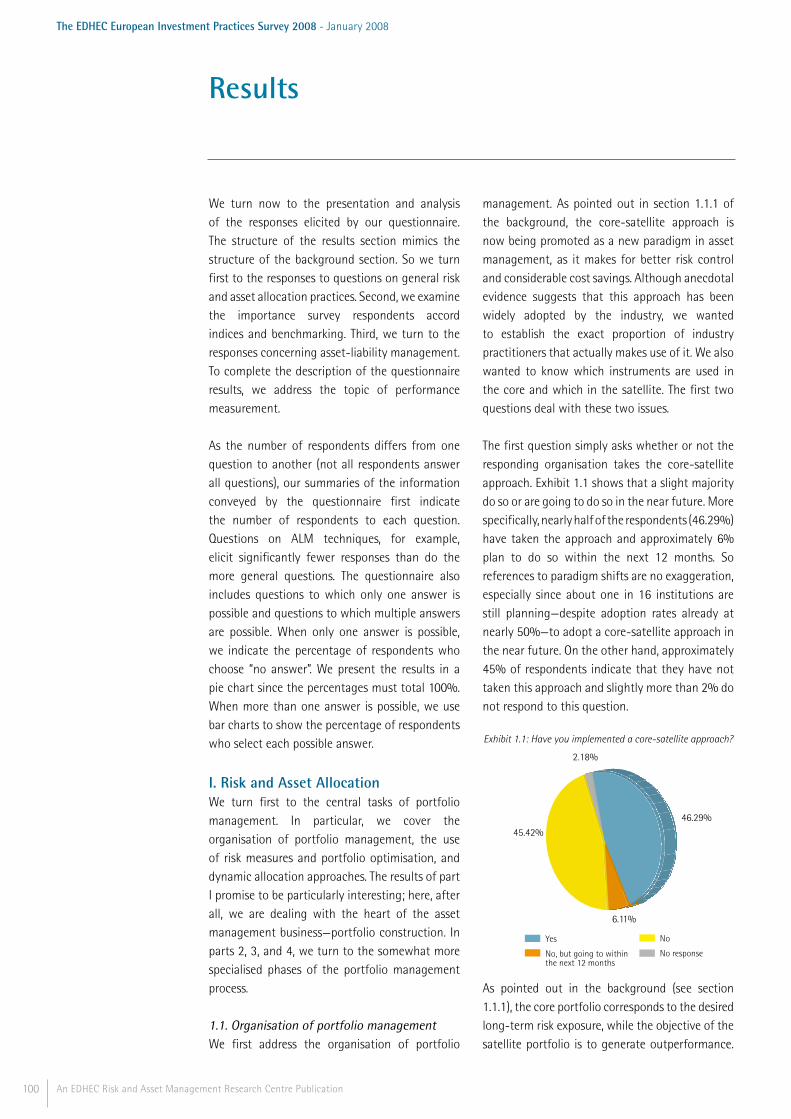
100 An EDHEC Risk and Asset Management Research Centre Publication
The EDHEC European Investment Practices Survey 2008 - January 2008
We turn now to the presentation and analysis of the responses elicited by our questionnaire. The structure of the results section mimics the structure of the background section. So we turn first to the responses to questions on general risk and asset allocation practices. Second, we examine the importance survey respondents accord indices and benchmarking. Third, we turn to the responses concerning asset-liability management. To complete the description of the questionnaire results, we address the topic of performance measurement.
As the number of respondents differs from one question to another (not all respondents answer all questions), our summaries of the information conveyed by the questionnaire first indicate the number of respondents to each question. Questions on ALM techniques, for example, elicit significantly fewer responses than do the more general questions. The questionnaire also includes questions to which only one answer is possible and questions to which multiple answers are possible. When only one answer is possible, we indicate the percentage of respondents who choose “no answer”. We present the results in a pie chart since the percentages must total 100%. When more than one answer is possible, we use bar charts to show the percentage of respondents who select each possible answer.
I. Risk and Asset Allocation We turn first to the central tasks of portfolio management. In particular, we cover the organisation of portfolio management, the use of risk measures and portfolio optimisation, and dynamic allocation approaches. The results of part I promise to be particularly interesting; here, after all, we are dealing with the heart of the asset management business—portfolio construction. In parts 2, 3, and 4, we turn to the somewhat more specialised phases of the portfolio management process.
1.1. Organisation of portfolio managementWe first address the organisation of portfolio
management. As pointed out in section 1.1.1 of the background, the core-satellite approach is now being promoted as a new paradigm in asset management, as it makes for better risk control and considerable cost savings. Although anecdotal evidence suggests that this approach has been widely adopted by the industry, we wanted to establish the exact proportion of industry practitioners that actually makes use of it. We also wanted to know which instruments are used in the core and which in the satellite. The first two questions deal with these two issues.
The first question simply asks whether or not the responding organisation takes the core-satellite approach. Exhibit 1.1 shows that a slight majority do so or are going to do so in the near future. More specifically, nearly half of the respondents (46.29%) have taken the approach and approximately 6% plan to do so within the next 12 months. So references to paradigm shifts are no exaggeration, especially since about one in 16 institutions are still planning—despite adoption rates already at nearly 50%—to adopt a core-satellite approach in the near future. On the other hand, approximately 45% of respondents indicate that they have not taken this approach and slightly more than 2% do not respond to this question.
Exhibit 1.1: Have you implemented a core-satellite approach?
Yes
No, but going to within the next 12 months
No
No response
46.29%
6.11%
45.42%
2.18%
As pointed out in the background (see section 1.1.1), the core portfolio corresponds to the desired long-term risk exposure, while the objective of the satellite portfolio is to generate outperformance.
Results

101An EDHEC Risk and Asset Management Research Centre Publication
The EDHEC European Investment Practices Survey 2008 - January 2008
A natural question to ask is which asset classes practitioners see as contributing to the long-term risk/return trade-off of their portfolio, and which they see as generators of outperformance that lead to tracking error with respect to the core. The question focuses on distinctions among four asset classes or investment approaches: indexed traditional investments (stocks and bonds), active traditional investments, hedge funds, and other alternative assets. Naturally, many would think of indexed stocks and bonds as the most popular choice for the core and the three other alternatives as the most popular for the satellite. However, as we note in the background (see section 1.2), indexed stock investments may be used as a satellite, either because the investor’s benchmark does not contain equity or because the investor wants to deviate from his strategic equity allocation in terms of styles, countries, or sectors and take on additional small-cap, value, or other exposure in the satellite. Alternative asset classes, on the other hand, may be attributed to the core if they serve to diversify the investor’s strategic allocation. Exhibit 1.2 shows how survey respondents position the four asset classes when it comes to the core-satellite approach. Broadly, the results show that traditional index funds are indeed the most popular investment support in the core portfolio (53.28% of respondents place them there), while hedge funds (placed in the satellite by roughly 38% of respondents) and other alternative assets (45%) are mainly seen as instruments for the satellite portfolio. It also appears that hedge funds and other alternative assets are considered assets that can be part of the core portfolio, with a significant fraction of respondents seeing them exclusively in the core (13.54% and 8.30% respectively) and many respondents (approximately 28% and 24% respectively) see them as instruments for both core and satellite.
Making alternative investments part of the core is frequently recommended in the literature that focuses on optimal diversification of portfolios that incorporate alternative investments (Amenc,
Goltz, and Martellini 2005). For this reason, it is surprising that roughly 38% (45%) of investors still confine hedge funds (other alternative asset classes) to the satellite. The results also show that the potential use of traditional beta vehicles in the satellite portfolio is still admitted by only a minority of investors; indeed, approximately 53% of respondents confine these instruments to the core. It is with active traditional investments that survey respondents are at their most flexible (more than 34% consider these investments useful in both the core and the satellite). It should also be pointed out that nearly 23% see active traditional investments as part of the core portfolio. This latter positioning is clearly inconsistent with the basic principle of core-satellite portfolio management. While the main objective of core portfolio management is to improve the risk/return trade-off, this improvement is usually brought about through a long-term choice of risk factors, meaning allocation to several asset classes or styles. Venturing into a pure "bottom-up" or opportunistic approach as part of core management would mean renouncing any long-term risk strategy. It is therefore surprising that traditional active management, founded largely on stock-picking, is perceived as a component of the core portfolio by a significant fraction of respondents.
Exhibit 1.2: Within the core-satellite approach, which assets do you think should be included in the core/in the satellite/in both?
Core
Satellite
0
20
40
60
80
100
13.54%
38.43%
27.95%
20.09%
53.28%
8.73%
13.97%
24.02%
22.70%
21.40%
34.06%
21.84%
8.30%
44.54%
23.58%
23.58%
Both
No response
Hedge funds
Otheralternative
investments
Index funds or mandate (stocks and
bonds)Actively managed
funds or mandate (stocks and bonds)
Results
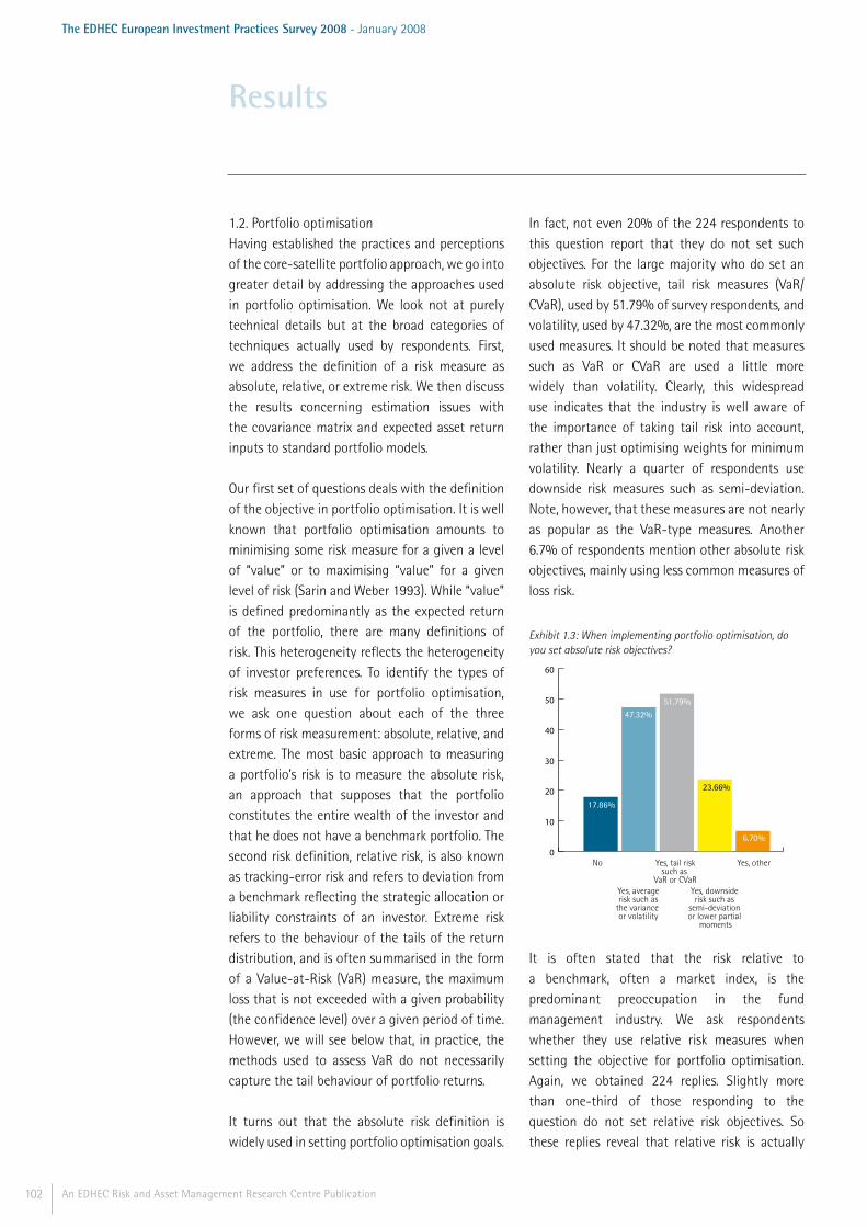
102 An EDHEC Risk and Asset Management Research Centre Publication
The EDHEC European Investment Practices Survey 2008 - January 2008
1.2. Portfolio optimisationHaving established the practices and perceptions of the core-satellite portfolio approach, we go into greater detail by addressing the approaches used in portfolio optimisation. We look not at purely technical details but at the broad categories of techniques actually used by respondents. First, we address the definition of a risk measure as absolute, relative, or extreme risk. We then discuss the results concerning estimation issues with the covariance matrix and expected asset return inputs to standard portfolio models.
Our first set of questions deals with the definition of the objective in portfolio optimisation. It is well known that portfolio optimisation amounts to minimising some risk measure for a given a level of “value” or to maximising “value” for a given level of risk (Sarin and Weber 1993). While “value” is defined predominantly as the expected return of the portfolio, there are many definitions of risk. This heterogeneity reflects the heterogeneity of investor preferences. To identify the types of risk measures in use for portfolio optimisation, we ask one question about each of the three forms of risk measurement: absolute, relative, and extreme. The most basic approach to measuring a portfolio’s risk is to measure the absolute risk, an approach that supposes that the portfolio constitutes the entire wealth of the investor and that he does not have a benchmark portfolio. The second risk definition, relative risk, is also known as tracking-error risk and refers to deviation from a benchmark reflecting the strategic allocation or liability constraints of an investor. Extreme risk refers to the behaviour of the tails of the return distribution, and is often summarised in the form of a Value-at-Risk (VaR) measure, the maximum loss that is not exceeded with a given probability (the confidence level) over a given period of time. However, we will see below that, in practice, the methods used to assess VaR do not necessarily capture the tail behaviour of portfolio returns. It turns out that the absolute risk definition is widely used in setting portfolio optimisation goals.
In fact, not even 20% of the 224 respondents to this question report that they do not set such objectives. For the large majority who do set an absolute risk objective, tail risk measures (VaR/CVaR), used by 51.79% of survey respondents, and volatility, used by 47.32%, are the most commonly used measures. It should be noted that measures such as VaR or CVaR are used a little more widely than volatility. Clearly, this widespread use indicates that the industry is well aware of the importance of taking tail risk into account, rather than just optimising weights for minimum volatility. Nearly a quarter of respondents use downside risk measures such as semi-deviation. Note, however, that these measures are not nearly as popular as the VaR-type measures. Another 6.7% of respondents mention other absolute risk objectives, mainly using less common measures of loss risk.
Exhibit 1.3: When implementing portfolio optimisation, do you set absolute risk objectives?
No
Yes, average risk such as the variance or volatility
Yes, tail risksuch as
VaR or CVaRYes, downside risk such as
semi-deviation or lower partial
moments
Yes, other0
10
20
30
40
50
60
17.86%
47.32%51.79%
23.66%
6.70%
It is often stated that the risk relative to a benchmark, often a market index, is the predominant preoccupation in the fund management industry. We ask respondents whether they use relative risk measures when setting the objective for portfolio optimisation. Again, we obtained 224 replies. Slightly more than one-third of those responding to the question do not set relative risk objectives. So these replies reveal that relative risk is actually
Results

103An EDHEC Risk and Asset Management Research Centre Publication
The EDHEC European Investment Practices Survey 2008 - January 2008
less widely used than absolute risk. Among the relative risk objectives used by respondents, tracking error volatility with respect to a benchmark, used by approximately half of the respondents (50.89%), is the most popular. Measures of tail risk with respect to a benchmark such as Value-at-Tracking-Error Risk account for nearly one-fifth of responses, followed by benchmark-relative downside risk, used by no more than approximately one in eight institutions. Slightly fewer than 3% of those responding to the question use other relative risk objectives, including measures such as the beta with respect to a benchmark.
In the context of portfolio allocation, absolute risk measures are more widely used than relative risk measures, a finding that weakens the claim that the definition of risk as relative risk is now the industry standard. However, when it comes to performance measurement, as opposed to portfolio optimisation, this claim may not be weakened at all (see part 4 for the survey findings on performance measurement). Remarkably, tail risk is not commonly taken into account when relative risk is being assessed, but it is when absolute risk is being assessed. To all appearances, the industry has not yet drawn on academic research results in the areas of asymmetric risk and tail risk and used it in the context of tracking error. The failure to do so is surprising, as it is straightforward to apply these concepts not just to simple returns but also to the returns in excess of a benchmark.
Exhibit 1.4: When implementing portfolio optimisation, do you set relative risk objectives with respect to a benchmark?
No
Yes, tracking error with respectto a benchmark
Yes, tail riskwith respect to
a benchmark such as Value-at-Tracking
error Risk
Yes, downside risk with respect to a benchmark,
such as semi-deviation
Yes, other(e.g., volatility
and beta)
0
20
40
60
80
67.16%
33.33%
14.22% 4.41%6.86%
While we have made it clear that extreme risk measures such as VaR and CVaR are widely used in portfolio optimisation, an interesting question is how extreme risk is assessed. As it happens, of the 219 respondents to this question, slightly more than a quarter (25.75%) report that they do not account for extreme risk at all. The most common method of calculating extreme risk measures (mentioned by 43% of respondents) is a method based on a normal distribution. It is most likely that this method owes its popularity to its simplicity and convenience. As mentioned in the background (see section 1.2.2), however, asset returns are generally not normally distributed. In addition, on the assumption of a normal distribution, a VaR calculation does not add any information to the information on the mean return and the volatility, since the distribution is completely characterised by these two parameters. Consequently, incorporating deviations from normality into the VaR measure is critical. However, our survey shows that only a small minority of respondents account for the deviations from normality of portfolio return distributions: 17.35% use a VaR calculation that accounts for higher moments through approximations and less than 10% use VaR calculations based on explicit modelling of the tail distribution through extreme value theory. Conditional Value-at-Risk (CVaR)—for technical reasons it is often seen as a preferred risk objective—is considerably less likely to be used (chosen as it is by 23.29% of respondents) than VaR (CVaR can be a more convex objective; see Rockafellar and Uryasev 2000). Also note that CVaR may provide a more appropriate characterisation of investor risk preferences, as it takes into account the magnitude of losses beyond VaR. Roughly 13% of respondents report that they use other methods to calculate extreme risk. Among these are stress-testing, the most common answer, followed by methods such as scenario-based, historic, Monte Carlo, and filtered bootstrapping Value-at-Risk.
Results
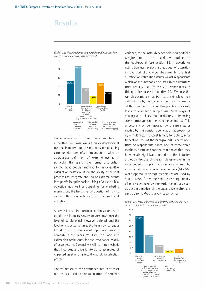
104 An EDHEC Risk and Asset Management Research Centre Publication
The EDHEC European Investment Practices Survey 2008 - January 2008
Exhibit 1.5: When implementing portfolio optimisation, how do you calculate extreme risk measures?
Do notaccount for
this
Value-at Riskbased on a
normaldistribution
Value-at-Riskthat accounts for higher moments through
approximations (e.g., Cornish-Fisher VaR)
Value-at-Riskbased on extreme
value theory
Other (e.g., stress-testing, scenario, historic return,
filtered bootstrapping)
ConditionalValue-at-Risk
(CVaR)
0
10
20
30
40
50
8.68%
23.29%
13.24%
17.35%
42.92%
25.75%
The recognition of extreme risk as an objective in portfolio optimisation is a major development for the industry, but the methods for assessing extreme risk are often inconsistent with an appropriate definition of extreme events. In particular, the use of the normal distribution as the most popular method for Value-at-Risk calculation casts doubt on the ability of current practices to integrate the risk of extreme events into portfolio optimisation. Using a Value-at-Risk objective may well be appealing for marketing reasons, but the fundamental question of how to evaluate this measure has yet to receive sufficient attention.
A central task in portfolio optimisation is to obtain the input necessary to compute both the level of portfolio risk, however defined, and the level of expected returns. We turn now to issues linked to the estimation of input necessary to compute these measures. First, we look into estimation techniques for the covariance matrix of asset returns. Second, we will turn to methods that incorporate uncertainty as to estimates of expected asset returns into the portfolio selection process.
The estimation of the covariance matrix of asset returns is critical to the calculation of portfolio
variance, as the latter depends solely on portfolio weights and on this matrix. As outlined in the background (see section I.2.1), covariance estimation has received a great deal of attention in the portfolio choice literature. In the first question on estimation issues, we ask respondents which of the methods discussed in the literature they actually use. Of the 204 respondents to this question, a clear majority—67.16%—use the sample covariance matrix. Thus, the simple sample estimator is by far the most common estimator of the covariance matrix. This practice obviously leads to very high sample risk. Most ways of dealing with this estimation risk rely on imposing some structure on the covariance matrix. This structure may be imposed by a single-factor model, by the constant correlation approach, or by a multifactor forecast (again, for details, refer to section I.2.1 of the background). Exactly one-third of respondents adopt one of these three methods, a rate of adoption that shows that they have made significant inroads in the industry, although the use of the sample estimator is far more common. Implicit factor models are used by approximately one in seven respondents (14.22%), while optimal shrinkage techniques are used by about 4.5%. Other methods, consisting mainly of more advanced econometric techniques such as dynamic models of the covariance matrix, are used by some 7% of survey respondents.
Exhibit 1.6: When implementing portfolio optimisation, how do you estimate the covariance matrix?
Use of the sample
covariance matrix
Specify a model with explicit factors, such as single-factor
model, constant correlation approach
of multifactor forecast
Implicit factor models
(e.g., use of PCA)
Use of optimal of shrinkage techniques
Other (Monte Carlo, autoregressive
models)
0
10
20
30
40
50
60
70
80
4.41% 6.86%
14.22%
33.33%
67.16%
Results
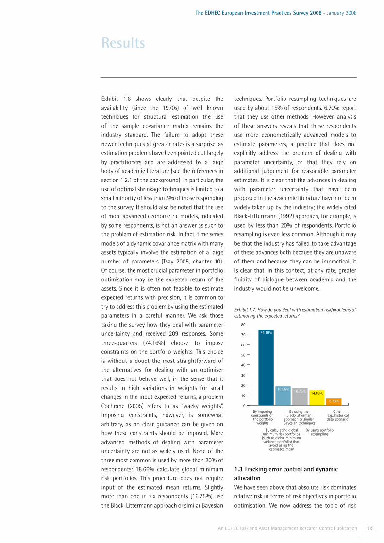
105An EDHEC Risk and Asset Management Research Centre Publication
The EDHEC European Investment Practices Survey 2008 - January 2008
Exhibit 1.6 shows clearly that despite the availability (since the 1970s) of well known techniques for structural estimation the use of the sample covariance matrix remains the industry standard. The failure to adopt these newer techniques at greater rates is a surprise, as estimation problems have been pointed out largely by practitioners and are addressed by a large body of academic literature (see the references in section 1.2.1 of the background). In particular, the use of optimal shrinkage techniques is limited to a small minority of less than 5% of those responding to the survey. It should also be noted that the use of more advanced econometric models, indicated by some respondents, is not an answer as such to the problem of estimation risk. In fact, time series models of a dynamic covariance matrix with many assets typically involve the estimation of a large number of parameters (Tsay 2005, chapter 10). Of course, the most crucial parameter in portfolio optimisation may be the expected return of the assets. Since it is often not feasible to estimate expected returns with precision, it is common to try to address this problem by using the estimated parameters in a careful manner. We ask those taking the survey how they deal with parameter uncertainty and received 209 responses. Some three-quarters (74.16%) choose to impose constraints on the portfolio weights. This choice is without a doubt the most straightforward of the alternatives for dealing with an optimiser that does not behave well, in the sense that it results in high variations in weights for small changes in the input expected returns, a problem Cochrane (2005) refers to as “wacky weights”. Imposing constraints, however, is somewhat arbitrary, as no clear guidance can be given on how these constraints should be imposed. More advanced methods of dealing with parameter uncertainty are not as widely used. None of the three most common is used by more than 20% of respondents: 18.66% calculate global minimum risk portfolios. This procedure does not require input of the estimated mean returns. Slightly more than one in six respondents (16.75%) use the Black-Littermann approach or similar Bayesian
techniques. Portfolio resampling techniques are used by about 15% of respondents. 6.70% report that they use other methods. However, analysis of these answers reveals that these respondents use more econometrically advanced models to estimate parameters, a practice that does not explicitly address the problem of dealing with parameter uncertainty, or that they rely on additional judgement for reasonable parameter estimates. It is clear that the advances in dealing with parameter uncertainty that have been proposed in the academic literature have not been widely taken up by the industry; the widely cited Black-Littermann (1992) approach, for example, is used by less than 20% of respondents. Portfolio resampling is even less common. Although it may be that the industry has failed to take advantage of these advances both because they are unaware of them and because they can be impractical, it is clear that, in this context, at any rate, greater fluidity of dialogue between academia and the industry would not be unwelcome.
Exhibit 1.7: How do you deal with estimation risk/problems of estimating the expected returns?
By imposingconstraints on the portfolio
weights
By calculating globalminimum risk portfolios (such as global minimum variance portfolio) that
avoid using the estimated mean
By using the Black-Litterman
approach or similar Bayesian techniques
By using portfolioresampling
Other (e.g., historical data, scenario)
0
10
20
30
40
50
60
70
80
14.83%
6.70%
16.75%18.66%
74.16%
1.3 Tracking error control and dynamic allocationWe have seen above that absolute risk dominates relative risk in terms of risk objectives in portfolio optimisation. We now address the topic of risk
Results

106 An EDHEC Risk and Asset Management Research Centre Publication
The EDHEC European Investment Practices Survey 2008 - January 2008
control. In this context of monitoring investments with respect to the strategic benchmark, tracking error is likely to play a predominant role. We discuss below the instruments and techniques for relative risk control that, as revealed by our survey, are currently favoured by the industry.
Approximately half of the 219 respondents who answer this question (47.95%) confirm that they define risk budgets in terms of tracking error. In fact, the percentage of those surveyed who use tracking error to monitor risk budget compliance is comparable to that of those who use volatility in portfolio optimisation, which is obviously a standard technique. Optimising a manager portfolio subject to constraints on risk factor exposure to ensure that tracking error is respected, a method used by a quarter of respondents, is also very popular. It is somewhat surprising that this method is so popular, as it has numerous drawbacks and can in fact be altogether infeasible, as pointed out in the background (section 1.3.2). Furthermore, our survey clearly reflects the increasing use of portable alpha. In fact, more than 20% of respondents report that they use portable alpha vehicles with zero beta exposure for purposes of tracking error control. This percentage, however, is significantly lower than the percentage of respondents who take the core-satellite approach. It is somewhat surprising that, while about half the respondents subscribe to core-satellite portfolio management (see exhibit I.1), little more than 20% use portable alpha strategies, which allow the most clear-cut separation of alpha and beta. Despite their great flexibility when it comes to relative risk control, completeness portfolios are used by only one in eleven respondents. Approximately 27% of respondents report that they do not use any such mechanism to control relative risk. In short, it appears that the importance of controlling relative risk is widely acknowledged, as a large majority of respondents use at least one of the methods that make this risk control possible. However, the clearest and most flexible methods of controlling relative risk—completeness portfolios and portable
alpha overlays—are used by only a minority of respondents, even though a majority favour a core-satellite portfolio approach.
Exhibit 1.8: For purposes of relative risk control, do you use the following?
Definition ofa risk budget in
terms of tracking error
Completenessportfolio to
neutralise factorexposures of active
managers
Portable alphavehicles with
zero beta exposure
Optimisation of manager portfolios
subject to constraintson risk factor exposure
None of the above
0
10
20
30
40
50
25.11%26.94%
21.46%
8.68%
47.95%
We have addressed the issue of portfolio optimisation in some detail above (see section 1.2 and exhibits 1.3-1.7). Portfolio optimisation refers to the use of techniques to reap the benefits of diversification. Diversification, however, is but one of the methods of managing risk. A second and perhaps competing approach is to manage risk by buying some sort of insurance or hedging away this risk. This hedging is often achieved through the purchase of derivative products, or more generally, through structured investment strategies. Interestingly, it can be argued that a structured investment strategy based on hedging is the most general dynamic, as opposed to static, form of asset allocation. Our survey asks respondents whether they use these dynamic allocation strategies. Their answers are discussed below.
A large majority (61.68%) of the 214 who answer this question have not yet adopted any form of dynamic allocation strategy. Although these strategies are the most advanced form of risk management, the failure to adopt them at higher rates is hardly surprising, as the necessary expertise is more often to be found in the
Results

107An EDHEC Risk and Asset Management Research Centre Publication
The EDHEC European Investment Practices Survey 2008 - January 2008
investment bank arms of financial institutions than in asset management companies or institutional investors themselves. As a result, dynamic allocation strategies have been packaged into so-called structured products, which can then be used by investors as part of a static allocation approach they may be more comfortable with (Goltz, Martellini, and Simsek 2007). The findings of our survey suggest that this approach does not currently face competition from asset managers and investors who implement their own dynamic allocation strategies.
To shed light on the current use of dynamic strategies in the industry, we ask survey respondents what dynamic strategies they use and give them a choice of three commonly used strategies: constant proportion portfolio insurance (CPPI), option-based portfolio insurance (OBPI), and exotic option-based portfolio insurance (EOBPI). CPPI is a strategy that allocates assets dynamically over time in order to guarantee the capital invested. It requires two underlying assets, a risk-free asset and a risky asset. As pointed outin the background (section 1.3.3.1), CPPI dynamically allocates total assets to a risky asset in proportion to a multiple of the cushion, that is, the difference between current wealth and a desired protective floor. The remaining assets are then allocated to a risk-free asset. OBPI typically consists of an equity investment covered by a put option held in the same asset, to provide protection from adverse price movements. EOBPI is a similar strategy, but for the standard put option it substitutes a position in a path-dependent or exotic option such as a lookback option. In addition, some respondents mention variable proportion portfolio insurance (VPPI). This strategy is similar to the widely used CPPI strategy, but unlike the fixed multiplier in CPPI, the multiplier in the VPPI strategy is variable and actively managed, in the sense that it typically moves in tandem with expectations for the value of the risky asset—in other words, when the value of the risky asset is expected to rise the multiplier rises as well and when it is expected to fall the multiplier likewise falls.
Of course, strategies such as CPPI or VPPI require the implementation of a dynamic allocation strategy, while option-based portfolio insurance—OBPI or EOBPI—may be achieved with a derivatives contract. And although implementation issues are very different, a non-linear payoff profile is common to all of these strategies.
Moreover, asset managers and investors can implement these strategies directly or they can delegate the implementation to the provider of a structured product, who offers static access to the dynamic strategy.
Turning now to the responses, we see that nearly one-third of those answering this question (29.91%) use the traditional CPPI method, which is designed to ensure absolute performance. As only about 38% of respondents use any dynamic strategy at all, the dominance of CPPI is clear. Approximately 11% of respondents use the simple OBPI method and 6% use OBPI based on exotic options. Slightly more than 5% of respondents use other strategies, such as VPPI.
Exhibit 1.9: Which dynamic allocation strategies do you implement for non-linear beta management?
Simple constantproportionportfolio
insurance (CPPI)
Simple option-based portfolio
insurance (OBPI)
Option-basedportfolio insurance
(OBPI) based on exotic options
None
Other (e.g., VPPI)
0
10
20
30
40
50
60
70
80
61.88%
6.07%11.21%
29.91%
5.14%
These findings make it clear that dynamic allocation strategies are not widely used by the industry. When they are used, CPPI (29.91%) is far more popular than other strategies such as simple or exotic option-based portfolio insurance.
Results

108 An EDHEC Risk and Asset Management Research Centre Publication
The EDHEC European Investment Practices Survey 2008 - January 2008
The limited availability of liquid options on a wide range of underlyings may account for the greater popularity of CPPI. Interestingly enough, however, more unusual strategies such as EOBPI and VPPI make up a relatively large proportion of the dynamic strategies currently in use. EOBPI may be used because it can provide a large range of potentially path-dependent payoffs that may be tailored to specific client needs. The VPPI technique, in which the multiplier increases when the market goes up and decreases when market goes down, may lead to reverse results, as the change in the multiplier trails market movements. An alternative to the standard VPPI approach may be to condition the multiplier on information—market volatility, for example—rather than on past market movements.
2. Indices and BenchmarksWe have shown that the industry puts great emphasis on such sophisticated concepts as assessment of tail risk, portfolio optimisation involving a range of risk definitions, and risk budgeting. However, sophisticated methods of assessing this risk and of incorporating parameter uncertainty or dynamic weights into the investment process are used by only a minority of survey respondents. After examining general techniques used as part of the portfolio management process, we look into a more specific aspect of investment management—the use of indices and benchmarks, the focus of this second part of our questionnaire. Our first aim is to show the types of indices that are actually used and the criteria on which the industry evaluates them. We also attempt to elucidate views of the numerous recent innovations in the indexing industry. Subsection two deals with new types of indices, including both indices for alternative asset classes and new forms of equity indexing.
2.1. Index use and quality requirements With the increasing variety of indices in the equity
universe, a logical first step in our survey is to show the published indices that respondents use as benchmarks for equity investments. We start with a focus on equity investment, as it is clearly the most significant area for indexing strategies. However, we do not merely ask those we survey to identify the categories of indices they use. We also ask them to report the percentage of assets under management (AUM) assigned to each of four categories of index: value-weighted indices, characteristics-based indices, equally-weighted indices, and other non-value-weighted indices. The first three are clearly the main categories of indices, and the fourth makes room for any indices we may have left out.
We note first the percentage of respondents using each category of index for more or less than 50% of their assets (see exhibit 2.1). These findings show the percentage of respondents for which a particular category of index is, for their investment purposes, a major or minor category. Another graph shows the average percentage of assets under management for these index categories (see exhibit 2.2). This double assessment makes it possible to determine the percentage of both users and assets garnered by a particular category of index. Showing only one or the other may hide interesting information. Results for assets under management indicate the average percentages of AUM covered by the index type only for the respondents who use the index type.
More than two-thirds of our complete sample of 229 respondents (70.74%) use value-weighted indices as benchmarks. For more than half the respondents (55.45%), this type of index accounts for coverage of more than 50% of assets under management. Despite the numerous drawbacks of value-weighting, value-weighted indices are still, to all appearances, the indices of choice for equity investment. Recall from the background (section 2.2) that these indices suffer from a lack of stable risk exposure and a lack of efficiency.Characteristics-based indices are regarded as
Results

109An EDHEC Risk and Asset Management Research Centre Publication
The EDHEC European Investment Practices Survey 2008 - January 2008
an important alternative to value-weighted indices. In these indices, firm characteristics such as dividend-yield, size, book-value, income, sales, and so on determine component weight. In recent years, a number of providers, including Wisdom Tree, Research Affiliates and its partner FTSE, and the American Stock Exchange have launched indices of this sort. Approximately one in six respondents currently use these characteristics-based indices as benchmarks. Most users of these indices apply them to less than 50% of their assets under management (15.29% of respondents); only a tiny fraction (1.75%) use characteristics-based indices as benchmarks for more than 50% of their assets under management.
Equally-weighted indices are another alternative to value-weighted indices. Equally-weighted indices are the average of the returns of their components. They give the same importance to the price movements of all the stocks they are made up of, so the price movements of every company in the index have the same impact on the value of the index. Claims have also been made for the lower purported risk of equally-weighted indices, as capitalisation weighting leads to high concentration in the few stocks with the highest market capitalisation (see background section 2.3.1.1 for details). In any case, approximately one-fifth (20.97%) of respondents use equally-weighted indices as benchmarks. However, they are used for more than 50% of assets under management by little more than 5% of respondents; for 16% of respondents, they are used as benchmarks for slightly less than half of AUM. In short, it turns out that equally-weighted indices are more popular than characteristics-based indices, as shown by the greater number of users who use them as benchmarks for the majority of AUM.
Other non-value-weighted indices make up the fourth and final category of indices. This category includes the indices that we do not further specify; it requires respondents to name the
additional indices they use. Those they mention include GDP-weighted indices, inflation-oriented indices, and fixed-mix benchmarks. GDP-weighted indices are international equity indices that, inspired by academic studies (Fama 1990) showing that macroeconomic factors do influence stock market returns, weigh the country components by GDP. Typically, the GDP weights are reset once a year and the portfolio is rebalanced accordingly (Hamza, Kortas, L’Her, and Roberge 2007). Country allocations are relatively stable because a country’s GDP does not vary considerably from one year to the next. These indices may be viewed as an alternative to the trend-following behaviour of value-weighted indices, at least as far as country allocations go. Fixed-mix indices consist of portfolios of stocks in which the initially attributed weights do not change over time. An equally-weighted index is a special case of a fixed-mix index with weights set equal to 1/N, where N is the number of stocks in the index. Defining weights different from 1/N while readjusting the fractions invested to keep weights stable irrespective of market movements also makes it possible to avoid the trend-following inherent to value-weighted indices. Finally, inflation-oriented indices are most commonly constructed from a consumer price index, often adding a constant return to the inflation rate. However, not even 7% of respondents use such non-value-weighted indices as benchmarks, making these additional alternatives considerably less popular than characteristics-based or equally-weighted indices. Exhibit 2.1 shows the details about the indices used for each type of index.
Results

110 An EDHEC Risk and Asset Management Research Centre Publication
The EDHEC European Investment Practices Survey 2008 - January 2008
Exhibit 2.1: Which published indices do you use as benchmark for your equity investments? Please indicate the percentage of assets under management for which each type of index is used as a benchmark.
Value-weightedindices
Characteristics-basedindices such as those
weighted by dividend-yield, sales, book-value, etc.
Other non-value-weighted indices
(such as GDP-weighted indices, inflation-oriented
indices and fixed-mix benchmarks)
Equal-weightedindices
15.29%
29.26%
1.75%
15.29%
82.97%
1.31%
5.68%
93.01%
79.04%
15.72%
5.25%
55.45%
0
20
40
60
80
100
Percentage of respondents for whomthe index type covers >50% of AUM
Percentage of respondents for whomthe index type covers <50% of AUM
Percentage of respondents with no replyfor the index type
Exhibit 2.2: The average percentage of assets under management for the above indices
Value-weightedindices
Characteristics-basedindices
Other non-value-weighted indices
(such as GDP-weighted indices, inflation-oriented
indices and fixed-mix benchmarks)
Equal-weightedindices
Average percentage of AUM covered by the index
0
10
20
30
40
50
60
70
80
24.38%
33.54%
27.56%
75.93%
Exhibit 2.2 indicates the results for the average assets under management. Recall that the averages are computed for respondents who report that they use the respective index type. Exhibit 2.2 makes it clear that, on average, users
of value-weighted indices benchmark the large majority of their assets to these indices. Users of other types of indices, however, benchmark only about one-quarter to one-third of their assets to these indices. Analysis of the percentages of assets under management assigned to each index type leads to the following conclusions. First, despite their severe problems, value-weighted indices are clearly dominant when it comes to equity investment. However, significant percentages of assets under management are also benchmarked to such alternative indexing forms as characteristics-based and equally-weighted indices. In addition, we note that equally-weighted indices (which account for 33.54% of AUM for the respondents using these indices) are slightly more popular than characteristics-based indices (accounting for 27.56% of AUM for the respondents using these indices).
Now that we have shown what indices are currently used by the industry, we look into its demands with respect to index quality. The main quality criteria we mention are transparency, efficiency, and stable risk exposure (see section 2.2 of the background for a detailed discussion of the quality requirements). Transparency (disclosure of the index construction methodology and of the current index composition), chosen as an essential criterion by slightly more than two-thirds (68.56%) of our 229 respondents, is clearly the primary requirement. As we note in the background (see section 2.2), stable risk exposure and efficiency are—if the index is to be used for asset allocation—also essential, but it seems that current practice does not attach much importance to these criteria. In fact, only 15.72% of respondents consider an efficient risk/return trade-off essential to a good index. Moreover, less than 8% of survey participants believe stable risk exposure to be essential to a good index.
Other characteristics viewed as essential to an index of good quality are mentioned by about 5% of respondents. The most frequently mentioned of these other characteristics is the popularity
Results

111An EDHEC Risk and Asset Management Research Centre Publication
The EDHEC European Investment Practices Survey 2008 - January 2008
and wide use of an index. Approximately 4% of respondents do not respond to the question.
Exhibit 2.3: Which characteristics do you consider essential for a good index?
Transparency (disclosure of the construction methodology or of the components)
Stable risk exposure
Efficient risk/return trade-off
Other (popularity, for example)
No response
68.56%
7.42%
15.72%
4.37%3.93%
The results reported above show that practitioners are more concerned with basic requirements such as the transparency and reputation of indices than with their risk and return properties. Risk and return properties can be divided into efficiency (in a mean-variance sense, for example) and stable risk exposure (such as exposure to styles, countries, and sectors). These are the two main qualities required of an index if it is to be a reasonable investment medium for asset allocation and a reasonable benchmark for performance measurement (see section 2.2 of the background). The survey findings suggest that existing indices are accepted without much criticism; only a minority of respondents consider efficiency essential. The purported efficiency of their indices is used as a major selling point by index providers, but it turns out that most index users do not consider it essential anyway.
We also ask respondents for their views on the problems with existing stock market indices (the question above attempts to show the criteria that are important, while the current question attempts to show the areas perceived as problematic). The
drawbacks of existing indices are thoroughly reviewed in the background (sections 2.2.1 and 2.2.2).
Nearly half (49.30%) of the 215 respondents who identify problems with broad stock market indices believe that these indices constitute momentum strategies that overweight good past performers and underweight bad past performers. Some 40% report that the assumptions of efficiency and of neutral risk choices are problematic. Some 3% mention other problems such as the influence of large outliers and lack of completeness. Only about one in eight (12.56%) report that they see no problems with broad stock market indices.
It thus appears that the problems of indices—their assumptions of efficiency and neutral risk exposure, in particular—are evident to the industry, an awareness that may account for the substantial use of alternative indices, as shown in exhibit 2.1. However, it should be noted that, while these problems are acknowledged, neither efficiency nor stable risk exposure is deemed a highly important criterion by respondents to our survey. It may be for this reason that despite their drawbacks standard value-weighted indices are still so widely used.
Exhibit 2.4: With regards to broad stock market indices, which do you consider problematic?
The assumption that these indices are
efficient
The assumption that these indices are
neutral choices
None
That these indices constitute momentum
strategies thatoverweight good past
performers and underweight bad past performers
Other (influence of large outliers,
lack of completeness, and so on)
2.79%
12.56%
49.30%
40.47%41.86%
0
10
20
30
40
50
Results
112 An EDHEC Risk and Asset Management Research Centre Publication
The EDHEC European Investment Practices Survey 2008 - January 2008
There is, however, a notable difference between these findings and the findings of an earlier survey discussed in the background (section 2.3.1.2 and exhibit 2.9). As it happens, the earlier survey, addressed to recipients of a report on the quality of stock market indices published by EDHEC in 2006,1 deals precisely with stock market indices. In this call for reactions, two-thirds of respondents report that inefficiency is the most serious problem with existing indices. And although approximately 13% of those responding to our current survey state that broad stock market indices are not problematic, less than 6% of those responding to the previous survey share this opinion.
Different survey samples may account for these different findings. The respondents to the earlier short survey had read EDHEC’s study of stock market indices. These respondents are likely to be more interested in market indices and to have thoroughly analysed index-related issues. Consequently, the sample consists of indexing specialists and practitioners with a strong focus on and experience of these problems. The present survey, by contrast, elicits opinions from a representative sample of industry practitioners. The present findings show that industry practitioners have a tendency to accept published indices without much criticism, on the grounds that they are transparent and branded. And, as is shown by the differences between the reactions of a sample of survey respondents with a particular interest in indices and those of a sample drawn from the entire industry, a sharper focus on stock market indices and their limitations would be of no little benefit to investment professionals as a group.
In short, survey respondents recognise the problems with indices (as shown in exhibit 2.4) but apparently do not consider them very important (as shown in exhibit 2.3). Current practice accepts existing stock market indices without questioning their quality to any significant extent. When asked explicitly to mention problems, however, a large majority of those in the industry do so.
-It is also surprising that the industry sets such store by index transparency rather than by risk and return properties—that is, efficiency and stability of risk exposure. While it is obviously necessary for a good index to be transparent, it is hardly sufficient. Indeed, it seems that a majority of the industry is willing to put up with completely inefficient and unstable indices on the grounds that they are transparent and popular. It is surprising that respondents emphasise quite straightforward criteria such as transparency rather than more important criteria such as efficiency, a criterion that determines whether or not capitalisation-weighted indices are a good investment choice in the first place.
2.2 Alternative indices: new indices and new asset classesAlthough there are many problems with value-weighted stock market indices, these indices are clearly the most firmly established in the financial industry. Recently, in the equity universe, there has been an increasing variety of indices, with new weighting methodologies, and an extension of indexing to asset classes such as hedge funds and real estate. In this section, we describe current industry perceptions of these emerging indices.
In the equity universe, there is a wide range of alternative index construction methodologies that compete with standard value weighting. Characteristics-based indices, weighted by variables such as firm size, book-value, income, and sales, are used for increasing amounts of assets and have been the focus of many recent media reports. In particular, the providers of indices that select and weight stocks by firm characteristics claim that over the long term these indices outperform value-weighted indices (see section 2.3.1.1 of the background, Arnott, Hsu, and Moore 2004, or Southard and Bond 2003). However, a lively debate has sprung up in the industry, with critics of these indices arguing that they are just value-tilted active strategies that outperform value-weighted indices over past periods but may suffer when value investing
Results
1 - Assessing the Quality of Stock Market Indices. EDHEC publication. 2006
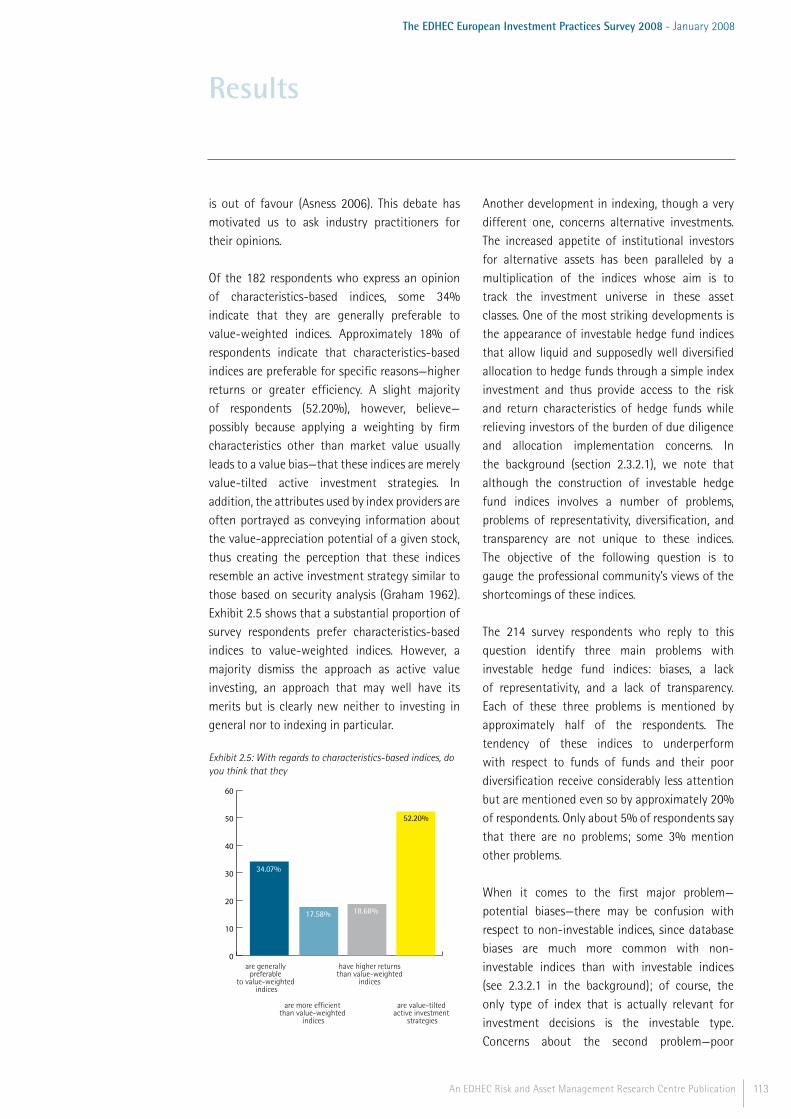
113An EDHEC Risk and Asset Management Research Centre Publication
The EDHEC European Investment Practices Survey 2008 - January 2008
is out of favour (Asness 2006). This debate has motivated us to ask industry practitioners for their opinions.
Of the 182 respondents who express an opinion of characteristics-based indices, some 34% indicate that they are generally preferable to value-weighted indices. Approximately 18% of respondents indicate that characteristics-based indices are preferable for specific reasons—higher returns or greater efficiency. A slight majority of respondents (52.20%), however, believe—possibly because applying a weighting by firm characteristics other than market value usually leads to a value bias—that these indices are merely value-tilted active investment strategies. In addition, the attributes used by index providers are often portrayed as conveying information about the value-appreciation potential of a given stock, thus creating the perception that these indices resemble an active investment strategy similar to those based on security analysis (Graham 1962). Exhibit 2.5 shows that a substantial proportion of survey respondents prefer characteristics-based indices to value-weighted indices. However, a majority dismiss the approach as active value investing, an approach that may well have its merits but is clearly new neither to investing in general nor to indexing in particular.
Exhibit 2.5: With regards to characteristics-based indices, do you think that they
are generally preferable
to value-weighted indices
are more efficient than value-weighted
indices
are value-tilted active investment
strategies
have higher returnsthan value-weighted
indices
0
10
20
30
40
50
60
52.20%
18.68%17.58%
34.07%
Another development in indexing, though a very different one, concerns alternative investments. The increased appetite of institutional investors for alternative assets has been paralleled by a multiplication of the indices whose aim is to track the investment universe in these asset classes. One of the most striking developments is the appearance of investable hedge fund indices that allow liquid and supposedly well diversified allocation to hedge funds through a simple index investment and thus provide access to the risk and return characteristics of hedge funds while relieving investors of the burden of due diligence and allocation implementation concerns. In the background (section 2.3.2.1), we note that although the construction of investable hedge fund indices involves a number of problems, problems of representativity, diversification, and transparency are not unique to these indices. The objective of the following question is to gauge the professional community’s views of the shortcomings of these indices.
The 214 survey respondents who reply to this question identify three main problems with investable hedge fund indices: biases, a lack of representativity, and a lack of transparency. Each of these three problems is mentioned by approximately half of the respondents. The tendency of these indices to underperform with respect to funds of funds and their poor diversification receive considerably less attention but are mentioned even so by approximately 20% of respondents. Only about 5% of respondents say that there are no problems; some 3% mention other problems.
When it comes to the first major problem—potential biases—there may be confusion with respect to non-investable indices, since database biases are much more common with non-investable indices than with investable indices (see 2.3.2.1 in the background); of course, the only type of index that is actually relevant for investment decisions is the investable type. Concerns about the second problem—poor
Results

114 An EDHEC Risk and Asset Management Research Centre Publication
The EDHEC European Investment Practices Survey 2008 - January 2008
representativity—are perhaps more legitimate: none of the existing investable indices can claim to be fully representative. The scarce data in the hedge fund universe may be partly responsible for this lack of representativity, but it is clear as well that none of the investable index providers explicitly includes the objective of representativity in its construction methodologies. Although methodologies that ensure representativity are in fact available (Goltz, Martellini, and Vaissié 2007), they have not been used in the industry. In the background (see 2.3.2.3) we note that an absence of transparency—the third major problem identified by survey respondents—also afflicts a range of other indices, such as standard stock market indices. Although transparency was listed as an important requirement for stock market indices (see exhibit 2.3), it was not frequently identified, interestingly enough, as one of the problems of these indices (see exhibit 2.4). Also note that only 4.67% of respondents believe there are no problems with hedge fund indices while 13% of respondents see no problems with stock market indices. It thus seems that on the strength of their brand names and their establishment status stock market indices escape the great scrutiny hedge fund indices are subjected to, as posited in section 2.3.2.1 of the background. Exhibit 2.6 shows the problems of investable hedge fund indices as identified by practitioners.
Exhibit 2.6: Which do you think is a problem when allocating money to investable hedge fund indices?
To conclude, the results show the importance of indices, as evidenced by their generally widespread use. In addition, and in spite of the dominance of value-weighted indices, a substantial proportion of respondents now use new forms of equity indices as benchmarks. Characteristics-based and equally-weighted indices emerge as the most popular alternatives. It should also be noted that survey respondents attribute relatively little importance to the risk and return qualities of standard stock market indices, emphasising instead brand reputation and transparency. On the other hand, they are considerably more critical of the newly emerging hedge fund indices. Overall, the survey results highlight both the important role of indices in the industry and the willingness to accept indices on the strength of their long history and their brand reputation. With increasing competition, however, it may well be that index providers will focus more on index quality in the sense of risk and return properties, potentially raising industry awareness of these quality issues.
3. Asset-Liability ManagementAsset-liability management (ALM) is an investment process that explicitly takes into account the investor’s liability constraints and aims to manage risk with respect to these constraints. ALM techniques are straightforward when, for example, they involve beating certain benchmarks rather than managing liability constraints. It may therefore be possible to use ALM techniques in the much broader context of benchmark-relative portfolio management. In the industry, however, it is only natural that the use of ALM techniques is limited to such liability-oriented investors as pension funds. In recent years, investors have been offered a range of product innovations, as noted in the background (see the box in section 3.1.1). In this part of the results, we show the extent to which the ALM approach has been adopted and the techniques that predominate. For a clear presentation of our results, we separate this part into two sections. The first section indicates the
Results
They are notrepresentative
They underperformwith respect tofunds of funds
Their constructionand/or compositionlack transparency
They are not sufficientlydiversified
There are no problems
They suffer biases such as survivorshipbias or backfilling
Other (e.g., theyexclude alpha
in fund-picking)
0
10
20
30
40
50
60
53.74%
21.96%
16.36%
46.73%
54.21%
4.67% 3.27%
115An EDHEC Risk and Asset Management Research Centre Publication
The EDHEC European Investment Practices Survey 2008 - January 2008
results concerning the basic concepts, as well as the techniques used in the analytical decision-making process. The second section turns to implementation issues, addressing the instruments and the assets used as investment media when putting ALM decisions into action.
3.1. ALM tools and techniques To specify the ALM techniques, the first fundamental question is to assess how many practitioners actually consider investment decisions within an ALM framework at all. 220 survey participants respond to this question. It turns out that nearly two-thirds (62.73%) of respondents do not use any form of ALM; instead, they work within a pure asset management perspective, without any consideration of liabilities. This finding is somewhat surprising, given the importance of taking into account liabilities in the investment process, as outlined in the background (see section 3.1). However, it may also be that the majority of the respondents to our survey are not subject to liability constraints (mutual funds or other managers of third-party assets, for example). Recall from the introduction that those surveyed fall into one of four categories: asset management companies, institutional investors/pension funds, private banks/family offices, and others (such as consulting companies and investment banks). For insight on whether the category the survey respondent falls into has any bearing on the adoption rates of ALM, we analyse the percentage of users per category. Unsurprisingly, we find that the percentage of respondents who do not use any ALM is highest (approximately 70%) for asset management/fund management companies. However, even for respondents in the institutional investors/pension fund category, this figure reaches 42%. Therefore, even though the overall low adoption is heavily influenced by the presence of third-party fund managers (note that this category accounts for nearly 55% of our survey sample; institutional investors, by contrast, account for only 24.02%), more than four in ten of the investors who are in principle liability-oriented (institutionals such as
pension funds) do not use ALM. It seems, in short, that current practice does not give liabilities the attention they merit.
We ask the respondents who do use ALM to identify the particular approach they use. Our survey identifies three approaches: cash-flow matching or immunisation, surplus optimisation, and liability-driven investment (LDI). We also include a specific form of LDI, non-linear risk-profiling. While the aim of cash-flow matching or immunisation is to create a risk-free asset to offset a potential shortfall, surplus optimisation involves finding an optimal trade-off between shortfall risk and return (surplus). Finally, LDI usually involves using standard building blocks to hedge against the duration and convexity risks, while keeping some assets free for investment in higher yielding asset classes. In ALM with non-linear risk-profiling, dynamic allocation techniques are used in an LDI framework. A detailed description of these approaches is provided in the background (section 3.1.1).
Exhibit 3.1 shows the results for the fundamental question on ALM. Of the minority of respondents who do use ALM, liability-driven investment and cash-flow matching/immunisation are the most popular approaches, with each being used by slightly less than one-fifth of respondents. With adoption rates of approximately 20%, LDI is the most popular approach in the industry, a finding that confirms that the current attention given to LDI in the press and at industry conferences is a clear reflection of the importance it has taken on in the market. However, cash-flow matching and immunisation, used by approximately 17% of respondents, are not far behind. In other words, the straightforward matching/immunisation approach is only slightly less popular than more recent LDI products. Surplus optimisation techniques are used by slightly more than 10% of respondents (11.36%). Non-linear risk-profiling as a specific LDI approach plays almost no role, used as it is by less than 3% of respondents.
Results
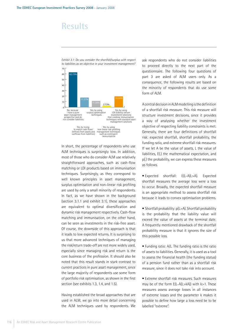
116 An EDHEC Risk and Asset Management Research Centre Publication
The EDHEC European Investment Practices Survey 2008 - January 2008
Exhibit 3.1: Do you consider the shortfall/surplus with respect to liabilities as an objective in your investment management?
No, because I have a pure
asset managementperspective and do
not consider liabilities
Yes, by trying to match cash flows
(inflows from assets andoutflows from liabilities)
Yes, by usingnon-linear risk-profiling
management techniques such as contingent
immunisation
Yes, by using surplus optimisation
techniques
Yes, by usingLDI (liability-driven
investment) solutions that combine immunisation
techniques with standard assetmanagement solutions
2.73%0
10
20
30
40
50
60
70
19.55%
11.36%17.27%
62.73%
In short, the percentage of respondents who use ALM techniques is surprisingly low. In addition, most of those who do consider ALM use relatively straightforward approaches, such as cash-flow matching or LDI products based on immunisation techniques. Surprisingly, as they correspond to well known principles in asset management, surplus optimisation and non-linear risk profiling are used by only a small minority of respondents. In fact, as we have shown in the background (section 3.1.1 and exhibit 3.1), these approaches are equivalent to optimal diversification and dynamic risk management respectively. Cash-flow matching and immunisation, on the other hand, can be seen as investments in the risk-free asset. Of course, the downside of this approach is that it leads to low expected returns. It is surprising to us that more advanced techniques of managing the risk/return trade-off are not more widely used, especially since managing risk and return is the core business of the profession. It should also be noted that this result stands in stark contrast to current practices in pure asset management, since the large majority of respondents use some form of portfolio risk optimisation, as shown in the first section (see exhibits 1.3, 1.4, and 1.5).
Having established the broad approaches that are used in ALM, we go into more detail concerning the ALM techniques used by respondents. We
ask respondents who do not consider liabilities to proceed directly to the next part of the questionnaire. The following four questions of part 3 are asked of ALM users only. As a consequence, the following results are based on the minority of respondents that do use some form of ALM.
A central decision in ALM modelling is the definition of a shortfall risk measure. This risk measure will structure investment decisions, since it provides a way of analysing whether the investment objective of respecting liability constraints is met. Generally, there are four definitions of shortfall risk: expected shortfall, shortfall probability, the funding ratio, and extreme shortfall risk measures. If we let A be the value of assets, L the value of liabilities, E(.) the mathematical expectation, and p(.) the probability, we can express these measures as follows.
• Expected shortfall: E(L-A|L>A). Expected shortfall measures the average loss were a loss to occur. Broadly, the expected shortfall measure is an appropriate method to assess shortfall risk because it leads to convex optimisation problems.
• Shortfall probability: p(L>A). Shortfall probability is the probability that the liability value will exceed the value of assets at the terminal date. A frequently mentioned drawback of the shortfall probability measure is that it ignores the size of this possible loss.
• Funding ratio: A/L. The funding ratio is the ratio of assets to liabilities. Generally, it is used as a tool to assess the financial health (the funding status) of a pension fund rather than as a shortfall risk measure, since it does not take risk into account.
• Extreme shortfall risk measures. Such measures may be of the form E(L-A|L>kA)) with k>1. These measures assess average losses in all instances of extreme losses and the parameter k makes it possible to define how large a loss need be to be labelled “extreme”.
Results

117An EDHEC Risk and Asset Management Research Centre Publication
The EDHEC European Investment Practices Survey 2008 - January 2008
Exhibit 3.2 indicates the popularity of these four measures as reported by those who respond to the question. Of those who use ALM techniques, a clear majority (62%) indicate that they use expected shortfall. The second most commonly used measure is shortfall probability, used by just under half of respondents. Expected shortfall is the preferred risk measure perhaps because, unlike shortfall probability, it takes into account the magnitude of the shortfall. More than one-third (35%) of respondents use the funding ratio; only about one-fifth use extreme shortfall risk measures. Interestingly, the percentage of extreme risk users in an ALM context is roughly equal to the percentage of respondents who use extreme risk measures in the context of benchmark-relative portfolio optimisation (see exhibit 1.4). In the general benchmark-relative context, and in the special case of a liability benchmark, extreme risk measures are far less common when it comes to assessing liability shortfall than they are when it comes to absolute risk optimisation. In fact, for portfolio optimisation with an absolute risk objective, extreme risk measures are used by more than 50% of respondents (see exhibit 1.3).
Exhibit 3.2: Which measures do you use in order to assess shortfall risk?
Expected shortfall
Shortfall probability
Extreme shortfall risk measure
Funding ratio
62.73%
0
10
20
30
40
50
60
70
80
19%
35%
49%
62%
After having assessed the major risk definitions in use in current practice, it is useful to find out how exactly risk analysis is carried out. Therefore, we proceed in a manner that is similar to the organisation of part 1 on risk and asset management techniques, and now continue with the techniques used to analyse risk.
In essence, ALM decision-making requires an assessment of outcomes that may occur over future horizons. Therefore, investment professionals require a model of future asset and liability values. This information will make it possible to infer the resulting funding ratio, shortfall probability, expected shortfall, and other risk measures for different investment decisions. So, to determine the optimal investment decision, a model of the future evolution of assets and liabilities is needed.
In principle, there are three possibilities for such a model. A first possibility is to analyse historical data. Investment decisions may be tested on historical prices and shortfall risk measures may be computed. Obviously, this possibility does not provide an extensive analysis of uncertainty, as only one specific outcome is taken into account. Nevertheless, slightly more than half of the respondents use this approach. It should be noted, however, that the answers to this question are not exclusive and we can conclude from the results below that in most cases further investigation complements simple historical analysis. A second approach is stress testing. Stress testing consists of simulating extreme conditions to test their impact on ALM portfolios. A common test involves analysing the impact of a steep rise in interest rates. Stress-testing, used by exactly two-thirds of the survey respondents who identify the models they use for ALM decisions, is the most popular method for modelling the future evolution of assets and liabilities. The third way of modelling future uncertainty is scenario generation. This method is based on explicitly characterising a range of future outcomes, which may then be fed into a decision-making process, such as an optimisation method.
A number of methods can be used to generate scenarios. First, it is possible to use a qualitative method in which scenarios are generated based on the judgement of experts. An advantage of this method is that the scenarios correspond to outcomes that may be characterised intuitively.
Results
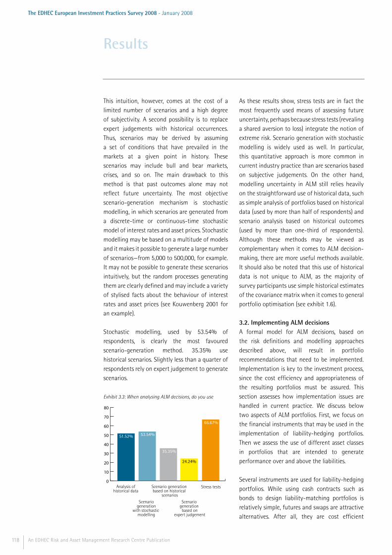
118 An EDHEC Risk and Asset Management Research Centre Publication
The EDHEC European Investment Practices Survey 2008 - January 2008
This intuition, however, comes at the cost of a limited number of scenarios and a high degree of subjectivity. A second possibility is to replace expert judgements with historical occurrences. Thus, scenarios may be derived by assuming a set of conditions that have prevailed in the markets at a given point in history. These scenarios may include bull and bear markets, crises, and so on. The main drawback to this method is that past outcomes alone may not reflect future uncertainty. The most objective scenario-generation mechanism is stochastic modelling, in which scenarios are generated from a discrete-time or continuous-time stochastic model of interest rates and asset prices. Stochastic modelling may be based on a multitude of models and it makes it possible to generate a large number of scenarios—from 5,000 to 500,000, for example. It may not be possible to generate these scenarios intuitively, but the random processes generating them are clearly defined and may include a variety of stylised facts about the behaviour of interest rates and asset prices (see Kouwenberg 2001 for an example).
Stochastic modelling, used by 53.54% of respondents, is clearly the most favoured scenario-generation method. 35.35% use historical scenarios. Slightly less than a quarter of respondents rely on expert judgement to generate scenarios.
Exhibit 3.3: When analysing ALM decisions, do you use
Analysis ofhistorical data
Scenariogeneration
with stochastic modelling
Scenario generation based on
expert judgement
Stress testsScenario generation based on historical
scenarios
0
10
20
30
40
50
60
70
80
24.24%
66.67%
35.35%
53.54%51.52%
As these results show, stress tests are in fact the most frequently used means of assessing future uncertainty, perhaps because stress tests (revealing a shared aversion to loss) integrate the notion of extreme risk. Scenario generation with stochastic modelling is widely used as well. In particular, this quantitative approach is more common in current industry practice than are scenarios based on subjective judgements. On the other hand, modelling uncertainty in ALM still relies heavily on the straightforward use of historical data, such as simple analysis of portfolios based on historical data (used by more than half of respondents) and scenario analysis based on historical outcomes (used by more than one-third of respondents). Although these methods may be viewed as complementary when it comes to ALM decision-making, there are more useful methods available. It should also be noted that this use of historical data is not unique to ALM, as the majority of survey participants use simple historical estimates of the covariance matrix when it comes to general portfolio optimisation (see exhibit 1.6).
3.2. Implementing ALM decisionsA formal model for ALM decisions, based on the risk definitions and modelling approaches described above, will result in portfolio recommendations that need to be implemented. Implementation is key to the investment process, since the cost efficiency and appropriateness of the resulting portfolios must be assured. This section assesses how implementation issues are handled in current practice. We discuss below two aspects of ALM portfolios. First, we focus on the financial instruments that may be used in the implementation of liability-hedging portfolios. Then we assess the use of different asset classes in portfolios that are intended to generate performance over and above the liabilities.
Several instruments are used for liability-hedging portfolios. While using cash contracts such as bonds to design liability-matching portfolios is relatively simple, futures and swaps are attractive alternatives. After all, they are cost efficient
Results
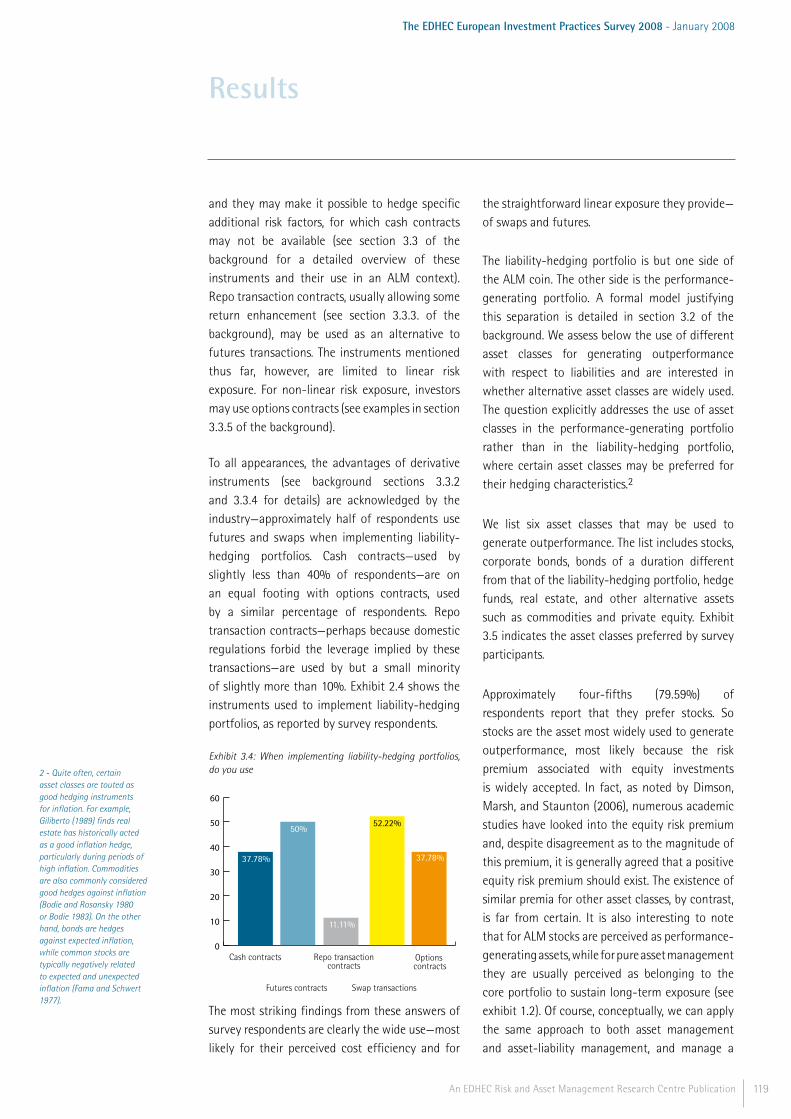
119An EDHEC Risk and Asset Management Research Centre Publication
The EDHEC European Investment Practices Survey 2008 - January 2008
and they may make it possible to hedge specific additional risk factors, for which cash contracts may not be available (see section 3.3 of the background for a detailed overview of these instruments and their use in an ALM context). Repo transaction contracts, usually allowing some return enhancement (see section 3.3.3. of the background), may be used as an alternative to futures transactions. The instruments mentioned thus far, however, are limited to linear risk exposure. For non-linear risk exposure, investors may use options contracts (see examples in section 3.3.5 of the background).
To all appearances, the advantages of derivative instruments (see background sections 3.3.2 and 3.3.4 for details) are acknowledged by the industry—approximately half of respondents use futures and swaps when implementing liability-hedging portfolios. Cash contracts—used by slightly less than 40% of respondents—are on an equal footing with options contracts, used by a similar percentage of respondents. Repo transaction contracts—perhaps because domestic regulations forbid the leverage implied by these transactions—are used by but a small minority of slightly more than 10%. Exhibit 2.4 shows the instruments used to implement liability-hedging portfolios, as reported by survey respondents.
Exhibit 3.4: When implementing liability-hedging portfolios, do you use
Cash contracts
Futures contracts Swap transactions
Options contracts
Repo transactioncontracts
0
10
20
30
40
50
60
52.22%
37.78%
11.11%
50%
37.78%
The most striking findings from these answers of survey respondents are clearly the wide use—most likely for their perceived cost efficiency and for
the straightforward linear exposure they provide—of swaps and futures.
The liability-hedging portfolio is but one side of the ALM coin. The other side is the performance-generating portfolio. A formal model justifying this separation is detailed in section 3.2 of the background. We assess below the use of different asset classes for generating outperformance with respect to liabilities and are interested in whether alternative asset classes are widely used. The question explicitly addresses the use of asset classes in the performance-generating portfolio rather than in the liability-hedging portfolio, where certain asset classes may be preferred for their hedging characteristics.2
We list six asset classes that may be used to generate outperformance. The list includes stocks, corporate bonds, bonds of a duration different from that of the liability-hedging portfolio, hedge funds, real estate, and other alternative assets such as commodities and private equity. Exhibit 3.5 indicates the asset classes preferred by survey participants.
Approximately four-fifths (79.59%) of respondents report that they prefer stocks. So stocks are the asset most widely used to generate outperformance, most likely because the risk premium associated with equity investments is widely accepted. In fact, as noted by Dimson, Marsh, and Staunton (2006), numerous academic studies have looked into the equity risk premium and, despite disagreement as to the magnitude of this premium, it is generally agreed that a positive equity risk premium should exist. The existence of similar premia for other asset classes, by contrast, is far from certain. It is also interesting to note that for ALM stocks are perceived as performance-generating assets, while for pure asset management they are usually perceived as belonging to the core portfolio to sustain long-term exposure (see exhibit 1.2). Of course, conceptually, we can apply the same approach to both asset management and asset-liability management, and manage a
Results
2 - Quite often, certain asset classes are touted as good hedging instruments for inflation. For example, Giliberto (1989) finds real estate has historically acted as a good inflation hedge, particularly during periods of high inflation. Commodities are also commonly considered good hedges against inflation (Bodie and Rosansky 1980 or Bodie 1983). On the other hand, bonds are hedges against expected inflation, while common stocks are typically negatively related to expected and unexpected inflation (Fama and Schwert 1977).

120 An EDHEC Risk and Asset Management Research Centre Publication
The EDHEC European Investment Practices Survey 2008 - January 2008
performance-generating portfolio relative to a long-term benchmark. The different uses in these two frameworks for the same type of asset may be explained by the definition of the benchmark, made up of the investor’s liabilities in ALM and often defined as a stock market index in pure asset management. Thus, our findings show that more often than not the choice of a benchmark is indeed a defining element of the investment process.
Alternative asset classes and alternative investment strategies have a strong position as well. Hedge funds are used by nearly half the respondents (48.98%), making them more popular than any other assets except stocks. Some 40% of respondents report using alternative assets such as real estate and other alternatives such as commodities and private equity. It is interesting to note that hedge funds and other alternative assets are commonly used both for pure asset management (see exhibit 1.2) and for ALM (see exhibit 3.5). Also, in pure asset management of core-satellite portfolios, these assets are found largely in the satellite (see exhibit 1.2), thus confirming the perception of alternative asset classes and investment strategies as vehicles for outperformance.
Exhibit 3.5: Which underlying assets do you prefer to use to generate performance to achieve a surplus with respect to liabilities?
Fixed-income instruments that deviate from the bond component of liabilities are another possible source of outperformance. Corporate bonds that
allow additional return by capturing a credit risk premium are included in outperformance generating portfolios by slightly less than half of respondents. Bond positions that may capture additional return but introduce additional risk through a deviation from the duration of liabilities are the least popular choice of all; the implication of this unpopularity is that investors are unwilling to compromise the liability-hedging properties of their overall portfolio. Overall, the results obtained from survey participants on asset-liability management indicate that ALM techniques are not as widely used in current practice as one might imagine. While these results are not surprising for the majority of respondents, made up of third-party money managers, it is certainly unexpected that nearly 40% of institutional investors do not currently consider potential liability shortfalls in their investment processes. It should be noted that in general asset management, a full 65% of respondents (see exhibit 1.4) consider benchmark-relative risk measures in portfolio optimisation. Therefore, our results suggest that asset-based benchmarks such as the well known stock market indices are of greater concern in current practice than are liability-based benchmarks. It appears to us that more focus is needed on liability-relative risk assessment and decision-making. Another salient finding is that despite their many advantages (see section 3.2 of the background) non-linear risk-profiling management techniques are almost entirely unexploited; indeed, only 2.73% of respondents make use of these techniques to manage shortfall risk in ALM. Interestingly, non-linear risk-management techniques are more common in general asset management, for which about 38% of respondents use some sort of dynamic allocation strategy. It is surprising that non-linear risk-management is not extended more frequently to shortfall risk management. A further notable finding is that measures of extreme risk, not widely used in ALM, are used by a majority of respondents in pure asset management. In fact, only 25.57% of respondents report in the general question on portfolio optimisation that they do not account for extreme risk (see section 1.2 and
Results
Stocks
Corporate bonds Hedge funds Other alternative assets such ascommodities,private equity
Real estateBonds of different duration than the liability
hedging portfolio
0
10
20
30
40
50
60
70
80
39.80%43.88%
29.59%
45.92%
79.59%
48.98%

121An EDHEC Risk and Asset Management Research Centre Publication
The EDHEC European Investment Practices Survey 2008 - January 2008
exhibit 1.5). A final noteworthy phenomenon is the extensive use, in ALM, of alternatives such as hedge funds and commodities for outperformance generation.
4. Performance Measurement and ReportingThe results above provide insight into current practices in managing and monitoring portfolio risk. While part I deals with the central tasks of risk and asset allocation, the following parts address more specific issues, in particular, indices and benchmarking and asset-liability management. Once the benchmark has been defined, the portfolio optimised, and risk controlled, it is important to assess the results. This ex post performance measurement is the topic of part 4. We look first at the use of such well known relative and absolute performance measures as the information and Sharpe ratios. Secondly, we assess the models currently used to analyse alpha. Finally, we turn to the topic of customised benchmarks and style analysis.
4.1. Use of performance measuresAt the beginning of part I, we assess the use of absolute and relative risk definitions in the context of portfolio optimisation. Here, we will take another look at the use of risk definitions, this time from the perspective of performance evaluation.
Absolute performance measures evaluate a portfolio’s risk-adjusted returns without any reference to a benchmark. We mention a variety of the most common absolute risk measures and ask respondents to identify those they use. The Sharpe ratio measures the return of a portfolio in excess of the risk-free rate, adjusted for the total risk of the portfolio, as measured by its standard deviation. Since this measure is based on the total risk, it makes it possible to evaluate portfolios that are not well diversified, as the unsystematic risk taken by the manager is included in this measure. On the other hand, the Treynor ratio, which
measures the relationship between the excess return on the portfolio and its systematic risk, is applicable to well diversified portfolios, since it takes only the systematic risk of the portfolio into account. Another well known indicator is the Sortino ratio. It is similar to the Sharpe ratio. However, the minimum acceptable return (MAR) replaces the risk-free rate and the standard deviation of the returns below the MAR replaces the standard deviation of all returns. VaR measures the maximum amount of loss in the portfolio for a given level of confidence (see details in section 4.1.1 of the background).
The Sharpe ratio is the most widely used measure, used as it is by approximately four-fifths of the 222 respondents who identify the absolute performance measures they use. Fewer than half of those responding use the average return in excess of the risk-free rate as an absolute performance measure. The downside and loss measures—the Sortino ratio and VaR—are each used by less than one-third of respondents. Only 11.26% of respondents use the Treynor ratio and only 4.5% report using other measures such as return in excess of a consumer price index (CPI), return to drawdown,3 or Omega ratios.4 These results are shown in exhibit 4.1.
Exhibit 4.1: To measure absolute performance, do you use
The clear dominance of the Sharpe ratio, used by four out of five respondents, comes as no surprise. After all, this measure, which has been in existence for more than forty years, is well known, easy to compute, and does not require any information
Results
3 - The return to drawdown compares the portfolio return with the largest drop from peak to valley during the period considered.4 - The Omega function captures all of the higher-moment information in the returns distribution. For any return level r, defined as the minimum acceptable return, the number Ω(r) is the probability-weighted ratio of gains to losses, relative to the threshold r (Keating and Shadwick 2002).
Sharpe ratio
Treynor ratio Measures basedon VaR
Other (return in excess of CPI,
return to drawdown and omega)
Average return inexcess of the risk-free rate
Sortino ratio
4.50%
0
10
20
30
40
50
60
70
80
43.24%
28.38%
11.26%
79.73%
29.73%

122 An EDHEC Risk and Asset Management Research Centre Publication
The EDHEC European Investment Practices Survey 2008 - January 2008
other than the series of portfolio returns. None of the other performance measures comes close to rivalling the popularity of the Sharpe ratio, despite its well known drawbacks. Indeed, this measure assumes that the distribution of portfolio returns is normal, i.e., that the moments with an order that is strictly greater than two are null. So this measure makes it impossible to take into account the asymmetry of the distribution, measured by the third moment (skewness), or the possible existence of fat tails, and consequently of extreme returns, which are evaluated by the fourth moment (kurtosis). It beggars belief that the average return in excess of the risk-free rate is used as a performance measure by more than 40% of respondents. In fact, this makes it the second most widely used performance measure. But the simple average return is not a performance measure at all, as it fails to account for risk. If more than 40% of respondents still use such simple measures, a greater focus on risk-adjusted performance measurement is clearly called for. Performance measures integrating the notion of downside risk are also relatively widely used. In fact, the Sortino ratio and VaR are each used by nearly 30% of respondents. These percentages, however, are low compared to the percentages of respondents who use these measures for portfolio optimisation: in part I, after all, we see that 75% of respondents use either VaR-type measures or downside risk measures as objectives in portfolio optimisation (see exhibit 1.3). Therefore, there seems to be a difference in the use of such measures, depending on whether the task at hand is portfolio optimisation or performance measurement. However, one may argue that portfolio optimisation is the area where the number of risk measures used may be more limited—in standard optimisation, it is necessary to set a single risk objective. In performance measurement, on the contrary, it may be useful to use a wide range of measures, wider even than that used in portfolio optimisation, to assess a given portfolio. For this reason, it is surprising that additional performance measures do not more frequently complement the standard Sharpe ratio.
We then identify the measures used to gauge relative performance. Relative risk measures evaluate a portfolio’s risk-adjusted returns using a reference to a benchmark. The possibilities we list in the questionnaire include Modigliani and Modigliani’s M-squared measure, the Graham Harvey measures, Jensen's alpha, the information ratio, adapted information ratios, and average return difference with a broad market index. Before turning to the results, a short description of these measures is in order. The information ratio is the residual return of the portfolio compared to its residual risk. In the standard information ratio risk is defined as tracking error volatility, but other risk definitions related to tracking error may also be used. Jensen's alpha is the difference between the excess return on the portfolio and the excess return explained by the market model. Modigliani and Modigliani’s M-squared, expressed in percentage terms, evaluates the annualised risk-adjusted performance (RAP) of a portfolio in relation to the market benchmark. The Graham Harvey measures are two. The first (GH1) is based on a leveraged/deleveraged benchmark portfolio that has the same volatility as the managed portfolio over the evaluation period. GH1 is the difference between the portfolio return and the return on the volatility-matched benchmark portfolio. The second, GH2, indicates the difference between the return on the leveraged/deleveraged managed portfolio that has the same volatility as the benchmark and the return on the benchmark. We leave further details on these performance measures to the background (see section 4.1) and turn now to the use of these measures in the industry.
214 survey respondents identify the relative performance measures they use. As indicated in exhibit 4.2, the information ratio, used by seven in ten respondents, prevails. It should be noted, however, that 7% of respondents, apparently realising the limitations of the standard information ratio, replace the tracking error volatility in the information ratio with a measure of asymmetric tracking error. More than one-third
Results
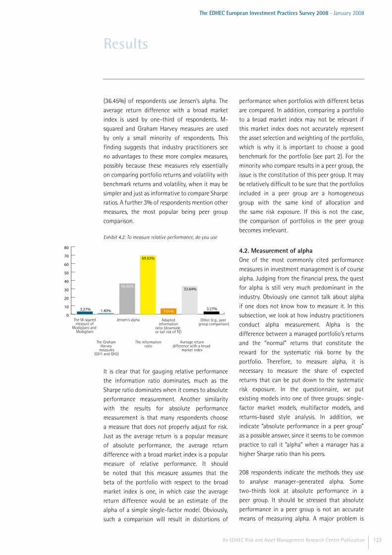
123An EDHEC Risk and Asset Management Research Centre Publication
The EDHEC European Investment Practices Survey 2008 - January 2008
(36.45%) of respondents use Jensen’s alpha. The average return difference with a broad market index is used by one-third of respondents. M-squared and Graham Harvey measures are used by only a small minority of respondents. This finding suggests that industry practitioners see no advantages to these more complex measures, possibly because these measures rely essentially on comparing portfolio returns and volatility with benchmark returns and volatility, when it may be simpler and just as informative to compare Sharpe ratios. A further 3% of respondents mention other measures, the most popular being peer group comparison.
Exhibit 4.2: To measure relative performance, do you use
It is clear that for gauging relative performance the information ratio dominates, much as the Sharpe ratio dominates when it comes to absolute performance measurement. Another similarity with the results for absolute performance measurement is that many respondents choose a measure that does not properly adjust for risk. Just as the average return is a popular measure of absolute performance, the average return difference with a broad market index is a popular measure of relative performance. It should be noted that this measure assumes that the beta of the portfolio with respect to the broad market index is one, in which case the average return difference would be an estimate of the alpha of a simple single-factor model. Obviously, such a comparison will result in distortions of
performance when portfolios with different betas are compared. In addition, comparing a portfolio to a broad market index may not be relevant if this market index does not accurately represent the asset selection and weighting of the portfolio, which is why it is important to choose a good benchmark for the portfolio (see part 2). For the minority who compare results in a peer group, the issue is the constitution of this peer group. It may be relatively difficult to be sure that the portfolios included in a peer group are a homogeneous group with the same kind of allocation and the same risk exposure. If this is not the case, the comparison of portfolios in the peer group becomes irrelevant.
4.2. Measurement of alphaOne of the most commonly cited performance measures in investment management is of course alpha. Judging from the financial press, the quest for alpha is still very much predominant in the industry. Obviously one cannot talk about alpha if one does not know how to measure it. In this subsection, we look at how industry practitioners conduct alpha measurement. Alpha is the difference between a managed portfolio’s returns and the “normal” returns that constitute the reward for the systematic risk borne by the portfolio. Therefore, to measure alpha, it is necessary to measure the share of expected returns that can be put down to the systematic risk exposure. In the questionnaire, we put existing models into one of three groups: single-factor market models, multifactor models, and returns-based style analysis. In addition, we indicate “absolute performance in a peer group” as a possible answer, since it seems to be common practice to call it “alpha” when a manager has a higher Sharpe ratio than his peers.
208 respondents indicate the methods they use to analyse manager-generated alpha. Some two-thirds look at absolute performance in a peer group. It should be stressed that absolute performance in a peer group is not an accurate means of measuring alpha. A major problem is
Results
The M-sqaredmeasure of
Modigliani and Modigliani
The Graham Harvey
measures(GH1 and GH2)
The informationratio
Average returndifference with a broad
market index
Adaptedinformation
ratio (downside or tail risk of TE)
Other (e.g., peer group comparison)
Jensen's alpha
1.40%3.27%0
10
20
30
40
50
60
70
80
69.63%
36.45%
7.01%
33.64%
3.27%
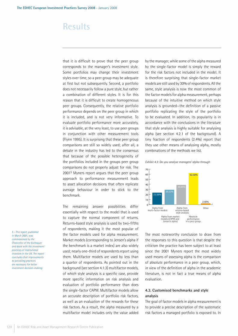
124 An EDHEC Risk and Asset Management Research Centre Publication
The EDHEC European Investment Practices Survey 2008 - January 2008
that it is difficult to prove that the peer group corresponds to the manager’s investment style. Some portfolios may change their investment styles over time, so a peer group may be adequate at first but not subsequently. Second, a portfolio does not necessarily follow a pure style, but rather a combination of different styles. It is for this reason that it is difficult to create homogeneous peer groups. Consequently, the relative portfolio performance depends on the peer group in which it is included, and is not very informative. To evaluate portfolio performance more accurately, it is advisable, at the very least, to use peer groups in conjunction with other measurement tools (Flynn 1995). It is surprising that these peer group comparisons are still so widely used; after all, a debate in the industry has led to the consensus that because of the possible heterogeneity of the portfolios included in the groups peer group comparisons do not properly adjust for risk. The 20015 Myners report argues that the peer group approach to performance measurement leads to asset allocation decisions that often replicate average behaviour in order to stick to the benchmark.
The remaining answer possibilities differ essentially with respect to the model that is used to capture the normal component of returns. Returns-based style analysis is used by two-fifths of respondents, making it the most popular of the factor models used for alpha measurement. Market models (corresponding to Jensen’s alpha if the benchmark is a market index) are also widely used; nearly one-third of respondents report using them. Multifactor models are used by less than a quarter of respondents. As pointed out in the background (see section 4.1.3) multifactor models, of which style analysis is a specific case, provide more specific information on risk analysis and evaluation of portfolio performance than does the single-factor CAPM. Multifactor models allow an accurate description of portfolio risk factors, as well as an evaluation of the rewards for these risk factors. As a result, the alpha measured by a multifactor model includes only the value added
by the manager, while some of the alpha measured by the single-factor model is simply the reward for the risk factors not included in the model. It is therefore surprising that single-factor market models are still used by 30% of respondents. All the same, style analysis is now the most common of the factor models for alpha measurement, perhaps because of the intuitive method on which style analysis is grounded—the definition of a passive portfolio replicating the style of the portfolio to be evaluated. In addition, its popularity is in accordance with the conclusions in the literature that style analysis is highly suitable for analysing alpha (see section 4.2.1 of the background). A tiny fraction of respondents (2.4%) report that they use other means of analysing alpha, mostly combinations of the methods we list.
Exhibit 4.3: Do you analyse managers’ alpha through
Alpha frommulti-factor models
Alpha from marketmodels (CAPM and
Jensen's alpha)
Absoluteperformance
in a peer group
OtherAlpha from returns-based style analysis
0
10
20
30
40
50
60
70
62.50%
2.40%
38.94%
29.33%23.56%
The most noteworthy conclusion to draw from the responses to this question is that despite the criticism the practice has been subject to at least since the 2001 Myners report the most widely used means of assessing alpha is the comparison of absolute performance in a peer group, which, in view of the definition of alpha in the academic literature, is not in fact a true means of alpha evaluation.
4.3. Customised benchmarks and style analysisThe goal of factor models in alpha measurement is to provide a precise description of the systematic risk factors a managed portfolio is exposed to. In
Results
5 - This report, published in March 2001, was commissioned by the Chancellor of the Exchequer and deals with the investment practices of institutional investors in the UK. The report concludes that improvements to prevailing practices are necessary for better investment decision-making.
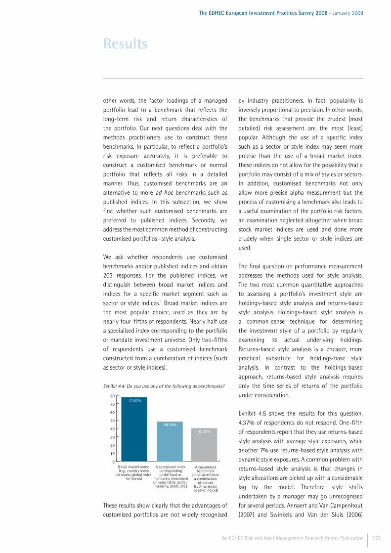
125An EDHEC Risk and Asset Management Research Centre Publication
The EDHEC European Investment Practices Survey 2008 - January 2008
other words, the factor loadings of a managed portfolio lead to a benchmark that reflects the long-term risk and return characteristics of the portfolio. Our next questions deal with the methods practitioners use to construct these benchmarks. In particular, to reflect a portfolio’s risk exposure accurately, it is preferable to construct a customised benchmark or normal portfolio that reflects all risks in a detailed manner. Thus, customised benchmarks are an alternative to more ad hoc benchmarks such as published indices. In this subsection, we show first whether such customised benchmarks are preferred to published indices. Secondly, we address the most common method of constructing customised portfolios—style analysis.
We ask whether respondents use customised benchmarks and/or published indices and obtain 203 responses. For the published indices, we distinguish between broad market indices and indices for a specific market segment such as sector or style indices. Broad market indices are the most popular choice, used as they are by nearly four-fifths of respondents. Nearly half use a specialised index corresponding to the portfolio or mandate investment universe. Only two-fifths of respondents use a customised benchmark constructed from a combination of indices (such as sector or style indices).
Exhibit 4.4: Do you use any of the following as benchmarks?
Broad market index (e.g., country index
for stocks, global index for bonds)
A customised benchmark
constructed from a combination
of indices (such as sector or style indices)
A specialised index correspondingto the fund or
mandate's investmentuniverse (style, sector, maturity, grade, etc.)
0
10
20
30
40
50
60
70
8077.83%
48.28%
40.39%
These results show clearly that the advantages of customised portfolios are not widely recognised
by industry practitioners. In fact, popularity is inversely proportional to precision. In other words, the benchmarks that provide the crudest (most detailed) risk assessment are the most (least) popular. Although the use of a specific index such as a sector or style index may seem more precise than the use of a broad market index, these indices do not allow for the possibility that a portfolio may consist of a mix of styles or sectors. In addition, customised benchmarks not only allow more precise alpha measurement but the process of customising a benchmark also leads to a useful examination of the portfolio risk factors, an examination neglected altogether when broad stock market indices are used and done more crudely when single sector or style indices are used.
The final question on performance measurement addresses the methods used for style analysis. The two most common quantitative approaches to assessing a portfolio’s investment style are holdings-based style analysis and returns-based style analysis. Holdings-based style analysis is a common-sense technique for determining the investment style of a portfolio by regularly examining its actual underlying holdings. Returns-based style analysis is a cheaper, more practical substitute for holdings-base style analysis. In contrast to the holdings-based approach, returns-based style analysis requires only the time series of returns of the portfolio under consideration. Exhibit 4.5 shows the results for this question. 4.37% of respondents do not respond. One-fifth of respondents report that they use returns-based style analysis with average style exposures, while another 7% use returns-based style analysis with dynamic style exposures. A common problem with returns-based style analysis is that changes in style allocations are picked up with a considerable lag by the model. Therefore, style shifts undertaken by a manager may go unrecognised for several periods. Annaert and Van Campenhout (2007) and Swinkels and Van der Sluis (2006)
Results

126 An EDHEC Risk and Asset Management Research Centre Publication
The EDHEC European Investment Practices Survey 2008 - January 2008
have recently shown that dynamic models for returns-based style analysis (RBSA) can use econometric tools to characterise the dynamics of style exposures and thus the evolution of style exposure over time.
As for holdings-based style analysis, 10% of respondents use fundamental style analysis, while another 9% use characteristics-based style analysis. The aim of fundamental style analysis is to match the asset allocation in terms of asset classes, while characteristics-based style analysis attempts to create a benchmark that matches certain characteristics (such as book-to-market ratio or dividend yields) of the managed portfolio (Lhabitant (2004).
The low information requirements of RBSA may account for its greater popularity. In fact, RBSA can be used when information on the composition of the portfolio is unavailable, making it much more convenient when the portfolio manager does not disclose portfolio holdings; after all, for holdings-based style analysis (HBSA) both the present and the historical composition of the portfolio, together with the weightings of the portfolio components, must be known with precision.
Exhibit 4.5: Do you use style analysis?
No
Yes, returns-based style analysis with average style exposures (e.g.,rolling window regression)
Yes, returns-based style analysis with dynamic style exposures (e.g., Kalman Filter)
Yes, holdings-based, fundamental style analysis(matching the allocation to asset classes)
Yes, holdings-based, characteristics-based style analysis (matching attributes such as book-to-market, dividend-yield, firm size)
No response
51.09%
18.34%
6.99%
10.48%
8.73%
4.37%
The results show that, in general, the returns-based approach is more popular than the holdings-based approach, although the latter, despite its numerous shortcomings, is nonetheless relatively popular. In particular, HBSA requires that the style characteristics of each security be identified and this style classification is often subjective, as it may be difficult to segregate growth and value. The difficulty of identifying the style of each asset leads to a potential reduction in the accuracy with which each position in the portfolio is known (Le Sourd 2006).
To conclude, industry practitioners largely use simple and well known measures to evaluate performance. However, their preference for these measures clearly leads to imprecise information on the risks and to inaccurate performance measurement and attribution. For example, the wide use of absolute performance in a peer group for alpha analysis means that there is no proper risk adjustment, as managers in the same peer group may deviate substantially from each other in terms of risk exposure. Likewise, the frequent use of average returns in excess of the risk-free rate or of the average excess return with respect to a broad market index as performance measures means that the risk exposures of the portfolios under analysis are altogether ignored. If the industry wants to make sophisticated risk analysis an integral part not only of portfolio optimisation but also of portfolio evaluation, an increased awareness of modern performance measurement techniques is clearly necessary.
Results

Conclusion
127An EDHEC Risk and Asset Management Research Centre Publication
128 An EDHEC Risk and Asset Management Research Centre Publication
The EDHEC European Investment Practices Survey 2008 - January 2008
The objective of the present survey is to gain an overview of the current practices in the industry. In particular, we set out to compare and potentially contrast current practices with the state of the art in the investment literature. To make this comparison, we first review state-of-the-art investment techniques in a background section and then focus on analysing the responses to our survey in a results section. Our questionnaire elicited responses from 229 European investment professionals. The regional coverage, as well as the coverage of firms of different sizes and types, allows us to conclude that our sample of respondents (made up primarily of asset managers and institutional investors, but also including private bankers and consultants) is representative of industry professionals.
The questionnaire deals with issues from four topics central to investment management: (i) risk and asset allocation (ii) indices and benchmarks (iii) asset-liability management (iv) performance measurement
Indeed, we cover a range of topics corresponding to the different areas of the investment process. It should be noted that the questions on asset-liability management are answered by a minority of overall respondents, as a focus on liabilities is not prevalent in the industry. Overall, however, the questions addressed to respondents are fairly general and focus on broad aspects of the investment process and on broad classifications of approaches rather than on technical details. Rather than concluding on a topic-by-topic basis, we provide below an overview of ten key conclusions that can be drawn from the findings across these four topics.
Assessment of Extreme Risk Taking into account tail risk is now a common practice in the industry, with a majority of respondents using measures such as VaR or CVaR in portfolio optimisation. It should be noted that the use of such measures is as common as the use of volatility as a risk measure. However, most respondents still rely on an assumption of
normal distribution when computing such measures. As the normal distribution is completely described by two parameters, the mean and the standard deviation of returns, this approach does not take into account extreme risk phenomena such as those that may be described by (non-trivial) skewness and excess kurtosis. Another interesting result is that measures of tail risk are not widely used in a relative risk context, such as tracking error risk or shortfall risk with respect to liabilities (neither is used by more than 20% of those responding to the questionnaire).
Portfolio OptimisationWhile portfolio optimisation is at the heart of investment management, our survey shows that current practice does not make extensive use of advanced techniques of input estimation and optimisation. In fact, the predominant approach to covariance estimation remains to use the sample estimator (used by about two-thirds of respondents). Likewise, advances such as the Black-Littermann approach or portfolio resampling, advances that allow the integration of estimation risk, are used by only a minority of survey respondents (less than 20%). More ad-hoc ways of avoiding estimation risk, such as imposing constraints on portfolio weights, are preferred.
Absolute Risk versus Relative RiskDespite the oft-mentioned importance of benchmarks, absolute definitions of risk prevail. For example, although approximately 35% of respondents do not consider relative risk measures in portfolio optimisation, not even 20% fail to consider absolute risk. Likewise, the most popular performance measures are absolute measures like the Sharpe ratio. Interestingly, even when asked for relative performance measures, a significant fraction of respondents report that absolute performance in a peer group is their preferred measure.
The Core-Satellite ApproachThe core-satellite approach is now widely adopted in practice, with more than 50% of respondents using
Conclusion
129An EDHEC Risk and Asset Management Research Centre Publication
The EDHEC European Investment Practices Survey 2008 - January 2008
it or planning to do so within the next 12 months. However, a number of inconsistencies remain; it is not clear that this new approach is being used to its full potential. Among these inconsistencies are those revealed by the findings on the use of different management approaches within core-satellite portfolios. For example, traditional active management is included in core portfolios, while alternative investments are largely confined to the satellite portfolio rather than used as diversifiers in the core. Moreover, it appears that the tracking error management methods that most clearly respect the separation of alpha and beta have not been widely adopted: portable alpha methods are used by only about 20% of respondents and the completeness portfolio approach by less than 10%.
Dynamic Asset AllocationA dynamic (as opposed to static) asset allocation strategy, encompassing diversification and hedging, can be viewed as the most general form of risk management, but this strategy is used by only a minority of those responding to our survey. And although dynamic asset allocation is used by 38% of respondents in a pure asset management context, only a small fraction (less than 3%) of liability-oriented investors report using this strategy in their ALM framework. Dynamic management of downside risk may be of even greater importance in ALM than in pure asset management, so the apparent failure of liability-oriented investors to take advantage of dynamic strategies is, to say the least, somewhat surprising.
IndicesThe survey results make it clear that traditional value-weighted indices maintain a very dominant position, in spite of the substantial attention accorded new forms of indexing. More often than not, the quality of value-weighted indices goes unquestioned; known brand names or high levels of transparency trump concerns about proven drawbacks such as inefficiency and instability. It should be noted, however, that, when explicitly asked, most respondents do recognise these drawbacks.
Asset-Liability ManagementA striking finding of the survey is that 42% of institutional investors do not consider liabilities at all. We see this failure to consider liabilities as further evidence of the excessive emphasis on asset-based benchmarks and of the insufficient emphasis on liabilities and the associated ALM techniques. For those respondents who do use ALM techniques, a simple use of historical data has a more important role (used by a majority of respondents) than that of explicit models of future uncertainty, which may be a more reliable basis for ALM decisions.
Performance MeasuresAnalysis of the performance measures currently used in the investment management industry shows that the Sharpe ratio (used by 80% of respondents) is the dominant measure of absolute performance and that the information ratio (used by 70% of respondents) is the dominant measure of relative performance. Measures incorporating downside or tail risk, by contrast, are used by only a minority of respondents. Limiting the analysis to such measures is obviously less than optimal because a wide range of measures, not necessarily excluding standard measures, may give a richer characterisation of a given portfolio. For this reason, it is surprising that the standard Sharpe and information ratios are not more frequently complemented by additional performance measures. Another striking finding is that measures of average return without any risk adjustment are more popular than all but the Sharpe and information ratios.
Analysis of AlphaAlpha analysis relies heavily on measures of absolute performance in a peer group. This is the predominant measure of alpha, used by nearly two-thirds of respondents, despite the fact that peer groups provide a very coarse adjustment for risk, leading to performance differences within the peer group that can be put down to investment style rather than to managerial skill. Style analysis, which allows precise adjustments with respect to style exposure, proves considerably less
Conclusion

130 An EDHEC Risk and Asset Management Research Centre Publication
The EDHEC European Investment Practices Survey 2008 - January 2008
popular but is nonetheless used by a significant minority of slightly less than 40% of respondents.
Customised BenchmarksCustomised benchmarks are the least popular of the available benchmarks, with only 40% of respondents reporting that they use them. Despite the more precise risk adjustment that customised benchmarks allow, broad market indices are clearly the benchmarks of choice, as they are used by nearly 80% of respondents. The second most popular choice is for indices specific to a particular sector or style that may correspond better to the actual risk exposure of a portfolio but that, compared to truly customised benchmarks, provide a rather crude description of risk-factor exposure. As they are not representative of portfolio allocation, the most widely used benchmarks create situations in which managers are rewarded as much for the performance of the markets in which their portfolios are invested as for their skill.
Concluding RemarksOverall, the results of our survey show that European asset managers and investors use a wide range of techniques that are often directly inspired by the literature on investment. However, we have ascertained that there is still a gap between the state of the art as described in this literature and the techniques actually used.
Our results suggest that this gap is particularly wide in the area of performance measurement. In fact, practitioner responses indicate that simple and well known measures are favoured in performance evaluation. As a result of industry preferences for these measures, investors must settle for imprecise information on the risks and for inaccurate performance measurement and attribution.
We find, for example, that the preferred measure of outperformance is absolute performance in a peer group, even though this measure is
unable to gauge with precision the risks of a given manager. More than 60% of respondents report that they use this approach. We have argued above that superior performance thus measured may stem simply from the asset class mix or investment style of the manager rather than from skill. More advanced techniques that gauge risk exposure precisely, such as alpha from returns-based style analysis, are not as widely used. In the same spirit of imprecision, almost 80% indicate that they use broad-based market indices for performance measurement, but only 40% customise benchmarks that truly reflect the risk exposure of the manager under evaluation. This finding is remarkable, as a broad index may in no way reflect the manager’s choices of risk exposure (industry sector, country, and investment style) and as the literature has found broad market indices to be inefficient portfolios with erratic exposure to underlying risk factors.
The most striking finding is that when makinginvestment decisions 42% of institutionalinvestors do not consider their liabilities at all.This finding is all the more surprising, in that the pension fund industry has just recovered from a crisis—driven by a decrease in plan assets and a simultaneous increase in liabilities—that clearly highlighted the importance of the interplay of assets and liabilities in pension fund management. Although it may be that liabilities are not always clearly defined, it would likely be worthwhile to define them rather than ignore them altogether. On the other hand, those investors who do use asset-liability management techniques use a wide range of techniques to model and manage future uncertainty, including surplus optimisation, immunisation, and modern LDI strategies. To our surprise, however, only 2.73% of respondents draw on non-linear risk profiling, despite its clear theoretical benefits.
In portfolio allocation, the gap between practice and theory is narrow when compared to the abyss separating the two in performance measurement. We find that European asset managers and
Conclusion

131An EDHEC Risk and Asset Management Research Centre Publication
The EDHEC European Investment Practices Survey 2008 - January 2008
investors use a range of optimisation techniques involving absolute, relative, and extreme risk measures. Furthermore, they take pragmatic approaches (setting weight constraints, computing global minimum risk portfolios) to avoid the “error maximisation” inherent to portfolio optimisers. However, more sophisticated estimation procedures, optimisation models, or dynamic allocation strategies are, for the moment, used by only a minority.
The most significant positive finding of our survey is on the non-technical front. Although we find that portfolio management and performance measurement practices fall short of the academic state of the art, there has been a profound paradigm change in investment practices, which is best reflected in the organisation of investment management rather than in its technical aspects. In particular, we have found that nearly half of all respondents have taken a core-satellite approach to their organisation of portfolio management. This approach recognises theinherent differences between choosing the benchmark of a portfolio and managing its outperformance. Thus, it corresponds to the conceptual distinction in the academic literature, while allowing considerable cost savings. A further point to note is that alternative investments, such as hedge funds, real estate, and commodities, now play a significant role in practical asset management. This clearly corresponds to academic recommendations that make the case for alternative diversification. We also note, however, that alternative investments are still mainly perceived as generators of outperformance rather than as portfolio diversifiers.
It appears that for much of the investment process practitioners prefer the most straightforward approaches, not fully exploiting a number of proven techniques that research has made readily available. But in other areas—the organisation of portfolio
management, for example—academic advances are clearly reflected. The EDHEC Risk and Asset Management Research Centre intends to continue monitoring industry practices—additional surveys are planned—in an attempt to gauge progress toward the closing of the gap between the availability of more advanced techniques and the industry use of these techniques.
Conclusion

132 An EDHEC Risk and Asset Management Research Centre Publication
The EDHEC European Investment Practices Survey 2008 - January 2008

References
133An EDHEC Risk and Asset Management Research Centre Publication

134 An EDHEC Risk and Asset Management Research Centre Publication
The EDHEC European Investment Practices Survey 2008 - January 2008
• Affleck-Graves, J. F., C. G. Troskie, and A. H. Money. 2002. A principal component index subject to constraints. Investment Analyst Journal 14 (4): April. • Alexander, C., and A. Dimitriu. 2003. Common trends, mean reversion and herding: sources of abnormal returns in equity markets. Discussion papers in finance. University of Reading. • Amenc, N., S. Curtis, and L. Martellini. 2003. The alpha and omega of hedge fund performance measurement. Working paper. EDHEC Risk and Asset Management Research Centre (January). • Amenc, N., and J. R. Giraud. 2005. Analysing alpha in performance measurement. http://www.edhec-risk.com/latest_news/Business%20_Strategy_Issues_RISKArticle.2005-06-02.1329?newsletter=yes. • Amenc, N., and F. Goltz. 2006. A reply to the CESR recommendations on the eligibility of hedge fund indices for investment of UCITS. EDHEC Risk and Asset Management Research Centre (December).
• Amenc, N., F. Goltz, and V. Le Sourd. 2006. Assessing the quality of stock market indices. EDHEC Publication. • Amenc, N., F. Goltz, and L. Martellini. 2005. Hedge funds from the institutional investor’s perspective. In Hedge Funds, Insights in Performance Measurement, Risk Analysis, and Portfolio Allocation. Edited by Gregoriou, G. N., G. Hübner, N. Papageorgiou, and F. Rouah. Wiley. • Amenc, N., and V. Le Sourd. 2003. Portfolio Theory and Performance Analysis. Wiley. • Amenc, N., P. Malaise, and L. Martellini. 2004. Revisiting core-satellite investing—a dynamic model of relative risk management. Journal of Portfolio Management 31 (1): 64-75. • Amenc, N., L. Martellini, and M. Vaissié. 2004. Indexing hedge fund indices. In Intelligent Hedge Fund Investing. Edited by Barry Schachter. London: RiskBooks. • Amenc, N., L. Martellini, and V. Ziemann. 2007. Asset-liability management decisions in household finance. Working paper. EDHEC Risk and Asset Management Research Centre. • Annaert, J., and G. Van Campenhout. 2007. Time variation in mutual fund style exposures. Review of Finance (forthcoming). • Arnott, R., J. Hsu, and P. Moore. 2004. Redefining indexation. Working paper. Research Affiliates. • Arnott, R.D., J. Hsu, and P. Moore. 2005. Fundamental indexation. Financial Analysts Journal 60 (2): 83-99. • Asness, C. 2006. The value of fundamental indexing. Institutional Investor Magazine 40 (10): 94-97 • Bailey, J. V. 1992. Are manager universes acceptable performance benchmarks? Journal of Portfolio Management 18 (3): 9-13. • Bailey, J. V., T. M. Richards, and D. E. Tierney. 1990. “Benchmark portfolios and the manager/plan sponsor relationship. In Current Topics in Investment Management. Edited by Fabozzi, F. J., and T. Dessa Fabozzi. New York: Harper Collins. • Barber, J., and M. Copper. 1996. Immunization using principal component analysis. Journal of Portfolio Management 23 (1): 99-105.
• Basak, S. 2002. A comparative study of portfolio insurance, Journal of Economic Dynamics and Control 26 (7-8):1217-1241.
References
135An EDHEC Risk and Asset Management Research Centre Publication
The EDHEC European Investment Practices Survey 2008 - January 2008
• Beltratti, A., A. Consiglio, and S. Zenios. 1999. Scenario modeling for the management of international bond portfolios. Annals of Operations Research 85:227–247. • Black, F., and R. Jones. 1987. Simplifying portfolio insurance. Journal of Portfolio Management 14 (fall): 48-51.
• Black, F., and R. Litterman. 1990. Asset allocation: combining investor views with market equilibrium. Goldman Sachs Fixed Income Research (September). • —. 1992. Global portfolio optimization. Financial Analysts Journal 48 (5): 28-43. • Black, F., and A. Perold, 1992. Theory of constant proportion portfolio insurance. Journal of Economic Dynamics and Control 16:403-426. • Bodie, Z. 1983. Commodity futures as a hedge against inflation. Journal of Portfolio Management Spring, 12-7. • Bodie, Z., and V. Rosansky. 1980. Risk and returns in commodity futures. Financial Analysts Journal (May/June): 27-39. • Boulier, J.-F., D. Florens, and E. Trussant. 1995. A dynamic model for pension fund management, In Proceedings of the 5th AFIR International Colloquium: 361-384. • Brennan, M. J. and E. S. Schwartz.1985. On the geometric mean index: a note. Journal of Financial and Quantitative Analysis 20 (1): 119-122. • Brinson, G. P., L. R. Hood, and G. L. Beebower. 1986. Determinants of portfolio performance Financial Analysts Journal 42 (July/August): 38-44. • Brinson, G. P., B. D. Singer, and G. L. Beebower. 1991. Determinants of portfolio performance II: an update. Financial Analysts Journal (47) (May/June): 40-48. • Brooks, C. and H. Kat. 2002. The statistical properties of hedge fund index returns and their implications for investors. Journal of Alternative Investments 5 (2). • Brown, S. J., W. Goetzmann, and R. Ibbotson. 1999. Offshore hedge funds: survival & performance 1989–95. Journal of Business 72 (1): 91–118. • Carhart, M. M. 1997. On persistence in mutual fund performance. Journal of Finance 52 (1): 57-82. • Cariño, D., T. Kent, D. Myers, C. Stacy, M. Sylvanus, A. Turner, K. Watanabe, and W. Ziemba. 1994. The Russell-Yasuda Kasai model: an asset/liability model for a Japanese insurance company using multistage stochastic programming. Interfaces 24:29–49. • Cariño, D., D. Myers, and W. Ziemba. 1998. Concepts, technical issues, and uses of the Russell-Yasuda Kasai financial planning model. Operations Research 46:450-462. • Cariño, D., and W. Ziemba. 1998. Formulation of the Russell-Yasuda Kasai financial planning model. Operations Research 46:433–449. • Chan, L. K. C., J. Karceski, and J. Lakonishok 1998. The risk and return from factors. Journal of Financial and Quantitative Analysis 33:159-88.
References
136 An EDHEC Risk and Asset Management Research Centre Publication
The EDHEC European Investment Practices Survey 2008 - January 2008
• —. 1999. On portfolio optimization: forecasting covariances and choosing the risk model. Review of Financial Studies 12:937-974.
• Chen, N.-F., R. Roll, and S. Ross. 1986. Economic forces and the stock market. Journal of Business 59 (3) : 383-403.
• Chopra, V., and W. Ziemba. 1993. The effect of errors in means, variances and covariances on optimal portfolio choice. Journal of Portfolio Management 19:6-11. • Cochrane, J. H. 1999. Portfolio advice for a multifactor world. Economic Perspectives 23 (3): 59-78. • —. 2005. A mean-variance benchmark for intertemporal portfolio theory. Working paper. University of Chicago. • Committee of European Securities Regulators. 2006. Can hedge fund indices be classified as financial indices for the purpose of UCITS? CESR’s issues paper (October). • Connor, G., and R. Korajczyk. 1986. Performance measurement with the arbitrage pricing theory: a new framework for analysis. Journal of Financial Economics 15:374-394. • —. 1993. A test for the number of factors in approximate factor models. Journal of Finance 48:1263-1291. • Cootner, P. 1972. Stock market indices: fallacies and illusions. In Modern Developments in Investment Management. Edited by Lorie, J., and R. Brealey. New York: Praeger. First published in Commercial and Financial Chronicle (September 29, 1966). • Cornish, E. A., and R. A. Fisher. 1937. Moments and cumulants in the specification of distributions. Review of the International Institute, 307-320. • DeRoon, F., T. Nijman, and J. ter Horst. 2000. Evaluating style analysis. Working paper. Quantitative Investment Research Europe. • diBartolomeo, D. and E. Witkowski. 1997. Mutual fund misclassification: evidence based on style analysis. Financial Analysts Journal (September-October). • Dimson, E., P. Marsh, and M. Staunton. 2002. Triumph of the Optimists. Princeton University Press. • —. 2006. The worldwide equity premium: a smaller puzzle. EFA 2006 Zurich meetings paper (April 7). • Draper, D., and D. Shimko. 1993. On the existence of “redundant securities”. Working paper. University of Southern California. • EDHEC. 2005. EDHEC European alternative diversification practices survey. EDHEC Risk & Asset Management Research Centre. • Elton, E., and M. Gruber. 1973. Estimating the dependence structure of share prices—implications for portfolio selection. Journal of Finance 28:1203-1232. • Elton, E. J., M. J. Gruber, S. Das, and M. Hlavka. 1993. Efficiency with costly information: a reinterpretation of evidence from managed portfolios. Review of Financial Studies 6 (1): 1-22. • Fabozzi, F., L. Martellini, and P. Priaulet. 2005. Hedging interest rate risk with term structure factor models. In The Handbook of Fixed-Income Securities, 7th edition. Edited by Fabozzi, F. John Wiley.
References

137An EDHEC Risk and Asset Management Research Centre Publication
The EDHEC European Investment Practices Survey 2008 - January 2008
• Fama, E. F. 1996. Multifactor portfolio efficiency and multifactor asset pricing. Journal of Financial and Quantitative Analysis 31 (4): 441-465.
• Fama, E. F., and K. R. French. 1992. The cross section of expected returns. Journal of Finance 47 (June): 427-465. • —. 1993. Common risk factors in the returns on stocks and bonds. Journal of Financial Economics 33:3-56. • —. 1995. Size and book-to-market factors in earnings and returns. Journal of Finance 50 (1): 131-155. • —. 1996. Multifactor explanations of asset pricing anomalies. Journal of Finance 51 (1): 55-81. • Fama, E. F., and G. W. Schwert. 1977. Asset returns and inflation. Journal of Financial Economics(November): 115-146. • Fedrigo, I., T. A. Marsh, and P. Pfleiderer. 1996. Estimating factor models of security returns: how much difference does it make? Working paper (December). • Feeney, G. J., and D. D. Hester. 1964. Stock market indices: a principal components analysis. Cowles Foundation discussion paper n° 175. • Fernholz, R., R. Garvy, and J. Hannon. 1998. Diversity-weighted indexing. Journal of Portfolio Management 24 (2): 74-82. • Fernholz, R., and B. Shay. 1982. Stochastic portfolio theory and stock market equilibrium. Journal of Finance 37 (2): 615-624. • Fisher, J., D. Gatzlaff, D. Geltner, and D. Haurin. 2003. Controlling for the impact of variable liquidity in commercial real estate price indices. Real Estate Economics 31: 269-303.
• Flynn M. 1995. Universes and peer groups: construction and use. Performance Evaluation, Benchmarks, and Attribution Analysis, AIMR. • Fung, W., and D. A. Hsieh. 2000. Performance characteristics of hedge funds and CTA funds: natural versus spurious biases. Journal of Financial and Quantitative Analysis 35 (3): 291-307. • —. 2001. The risk in hedge fund strategies: theory and evidence from trend followers. Review of Financial Studies 14 (2): 313-341. • —. 2004. Hedge fund benchmarks: a risk-based approach. Financial Analysts Journal (60) 5: 65-80. • Geltner, D. 1993. Estimating market values from appraised values without assuming an efficient market. The Journal of Real Estate Research 8 (3): 325-345. • Geyer, A., W. Herold, K. Kontriner, and W. Ziemba. 2001. The Innovest Austrian pension fund financial planning model InnoALM. Working paper. University of British Columbia. • Giliberto, S. 1989. Real Estate vs. Financial Assets: an Updated Comparison of Returns in the United States and the United Kingdom, New York: Salomon Brothers. • Goltz, F., L. Martellini, and K. Simsek. 2007. Optimal static allocation decisions in the presence of portfolio insurance. Journal of Investment Management (forthcoming).
References
138 An EDHEC Risk and Asset Management Research Centre Publication
The EDHEC European Investment Practices Survey 2008 - January 2008
• Goltz, F., L. Martellini, and M. Vaissié. 2007. Hedge fund indices: reconciling investability and representativity. European Financial Management 13 (2): 257-286. • Goltz, F., L. Martellini, and V. Ziemann. 2006. Exchange-traded fixed-income derivatives in asset management and asset-liability management. Journal of Fixed-Income 16 (1): 39-54. • Graham, B. 1962. Security Analysis: Principles and Technique. 4th ed., McGraw-Hill. • Graham, J. R., and C. R. Harvey. 1997. Grading the performance market-timing newsletters. Financial Analysts Journal (November/December) : 54-66. • Gregoriou, G., G. Hubner, N. Papageorgiou, and F. Rouah. 2005. Hedge funds from the institutional investor’s perspective. In Hedge Funds, Insights in Performance Measurement, Risk Analysis, and Portfolio Allocation. John Wiley & Sons. • Grinold, R. C., and R. N. Kahn. 2000. Active portfolio management: a quantitative approach for producing superior returns and controlling risk. 2nd ed. Irwin. • Hamza, O., M. Kortas, J. L’Her, and M. Roberge. 2007. International equity indices: exploring alternatives to market cap-weighting. Journal of Investing (summer): 103-118. • Haugen, R. A., and N. L. Baker. 1991. The efficient market inefficiency of capitalization-weighted stock portfolios. Journal of Portfolio Management 17 (3): 22-26. • Himmelblau, D. M. 1972. Applied Nonlinear Programming. New York: McGraw-Hill. • Hodges, S., and S. Schaefer. 1974. The interpretation of the geometric mean: a note. Journal of Financial and Quantitative Analysis 9 (3): 497-504. • Huberman, G., S. Kandel, and R. Stambaugh. 1987. Mimicking portfolios and exact arbitrage pricing. Journal of Finance 42 (1): 1-9. • Hsu, J. 2006. Cap-weighted portfolios are sub-optimal portfolios. Journal of Investment Management 4 (3): 1-10. • Hwang, S., and S. Satchell. 1999. Modelling emerging markets risk premia using higher moments. International Journal of Finance and Economics 4:271-296. • Ibbotson, R. G., and P. D. Kaplan. 2000. Does asset allocation policy explain 49, 90 or 100 percent of performance? Financial Analysts Journal (January/February). • Idzorek, T. M., and F. Bertsch. 2004. The style drift score. Journal of Portfolio Management 31 (1): 76-83. • Ippolito, R. 1989. Efficiency with costly information: a study of mutual fund performance, 1965-84. Quarterly Journal of Economics 104:1-23. • Jagannathan, R., and T. Ma. 2003. Risk reduction in large portfolios: why imposing the wrong constraints helps. Journal of Finance 58 (4): 1651-1683. • Jaschke, S. 2002. The Cornish-Fisher expansion in the context of delta-gamma-normal approximations. Journal of Risk 4:33-52. • Jegadeesh, N., and S. Titman. 1993. Returns to buying winners and selling losers: implications for stock market efficiency. Journal of Finance 48:65-91.
References
139An EDHEC Risk and Asset Management Research Centre Publication
The EDHEC European Investment Practices Survey 2008 - January 2008
• Jensen, M.C. 1968. The performance of mutual funds in the period 1945-1964. Journal of Finance 23 (May): 389-419.
• Johnstone, I. M. 2001. On the distribution of the largest eigenvalue in principal component analysis. Annals of Statistics 29:295-327.
• Jondeau, E., and M. Rockinger. 2004. Conditional volatility, skewness, and kurtosis: existence, persistence and comovements. Journal of Economic Dynamics and Control 27:1699-1737. • Jorion, P. 1985. International portfolio diversification with estimation risk. Journal of Business 58:259-278. • —. 1986. Bayes-Stein estimation for portfolio analysis. Journal of Financial and Quantitative Analysis 21 (3): 279-292. • Kahneman, D., and A. Tversky. 1979. Prospect theory: an analysis of decision under risk. Econometrica 47:263-291 • Kallberg, J., R. White, and W. Ziemba. 1982. “Short term financial planning under uncertainty. Management Science 28:670–682. • Keating, C., and W. Shadwick. 2002. A universal performance measure. Journal of Performance Measurement 6 (3): 59-84. • Kim, R., R. Shukla, and M. Thomas. 2000. Mutual fund objective misclassification. Journal of Economics and Business (July-August). • Kouwenberg, R. 2001. Scenario generation and stochastic programming models for asset-liability management. European Journal of Operational Research 127 (2): 279-292. • Kusy, M. and W. Ziemba. 1986. A bank asset and liability management model. Operations Research 34:356-376. • Laloux, L., J. P. Bouchard, P. Cizeau, and M. Potters. 1999. Random matrix theory. Risk Magazine 12 (3): 69. • Ledoit, O. 1999. Improved estimation of the covariance matrix of stock returns with an application to portfolio selection. Working paper. UCLA. • Lehmann, B., and D. Modest. 1987. Mutual fund performance evaluation: a comparison of benchmarks and benchmark comparisons. Journal of Finance 21 (233-65). • Leibowitz, M. and A. Weinberger. 1982. Contingent immunization—part I: risk control procedures. Financial Analysts Journal (November/December): 17–31. • —. 1983. Contingent immunization—part II: problem areas. Financial Analysts Journal (January/February): 35–50. • Lhabitant, F. S. 2004. Hedge Funds: Quantitative Insights. John Wiley & Sons. • —. 2007. Hedge fund indices for retail investors: UCITS eligible or not eligible? Derivatives Use, Trading and Regulation 12:275-289.
References

140 An EDHEC Risk and Asset Management Research Centre Publication
The EDHEC European Investment Practices Survey 2008 - January 2008
• Le Sourd, V., 2006, “A Question of Style”, Funds Europe, November
• Liang, B. 2001. Hedge fund performance: 1990-1999. Financial Analysts Journal (January/February): 11-18.
• Lintner, J. 1965. The valuation of risk assets and the selection of risky investments in stock portfolios and capital budgets. Review of Economics and Statistics (February): 13-37.
• Litterman, R., and J. Scheinkman. 1991. Common factors affecting bond returns. Journal of Fixed Income 1:54-61. • —. 1998. Estimating covariance matrices. Goldman, Sachs & Co. Risk Management Series (January). http://citeseer.ist.psu.edu/litterman98estimating.html.
• Lobosco, A., and D. diBartolomeo. 1997. Approximating the confidence intervals for Sharpe style weights. Financial Analysts Journal (July/August): 80-85. • Longstaff, F. A., and E. S. Schwartz. 1992. Interest rate volatility and the term structure: a two-factor general equilibrium model. Journal of Finance 47 (4): 1259-1282. • Lucas, L., and M. W. Riepe. 1996. The role of returns-based style analysis: understanding, implementing and interpreting the technique. Ibbotson Associates (May). • Malkiel, B. 1995. Returns from investing in equity mutual funds 1971 to 1991. Journal of Finance 50 (2) 549-572. • Marchenko, V., and L. Pastur. 1967. Eigenvalue distribution in some ensembles of random matrices. Mathematics of the USSR Sbornik 72:536-567. • Markowitz, H. 1952. Portfolio selection. Journal of Finance 7 (1): 77-91. • Martellini, L., P. Priaulet, and S. Priaulet. 2003. Fixed-Income Securities – Valuation, Risk Management and Portfolio Strategies. John Wiley. • Martellini, L., and V. Ziemann. 2005. Marginal impacts on portfolio distribution. Working paper. EDHEC Risk and Asset Management Research Centre. • —. 2006. The benefits of hedge funds in asset-liability management. Journal of Financial Risk Management 3 (2): 38-55. • —. 2007. Improved forecasts of higher order co-moments and implications for portfolio selection. EDHEC Risk and Asset Management Research Centre. • Merton, R. 1969. Lifetime portfolio selection under uncertainty: the continuous time case. Review of Economics and Statistics 51:247–257. • —. 1971. Optimum consumption and portfolio rules in a continuous time model. Journal of Economic Theory 3:373-413. • —. 1990. Continuous-Time Finance. Padstow, UK: Basil Blackwell. • Modigliani, F., and L. Modigliani. 1997. Risk-adjusted performance. Journal of Portfolio Management (winter): 45-54.
References
141An EDHEC Risk and Asset Management Research Centre Publication
The EDHEC European Investment Practices Survey 2008 - January 2008
• Mulvey, J., F. Fabozzi, W. Pauling, K. Simsek, and Z. Zhang. 2005. Modernizing the defined-benefit pension system. Journal of Portfolio Management 31 (2): 73-82. • Mulvey, J., G. Gould, and C. Morgan. 2000. The asset and liability management system for Towers Perrin-Tillinghast. Interfaces 30:96–114.
• Mulvey, J., and H. Vladimirou. 1992. Stochastic network programming for financial planning problems. Management Science 38:1642–1664. • Posthuma, N. and P. J. Van der Sluis. 2003. A reality check on hedge fund returns. Unpublished paper.
• Ranaldo, A., and R. Häberle. 2006. Wolf in sheep’s clothing: the active investment strategies behind index performance. Working paper. UBS AG. • Rockafellar, R. T., and S. Uryasev. 2000. Optimization of Conditional Value-at-Risk. Journal of Risk 2 (3): 21-41. • Roll R. 1977. A critique of the asset pricing theory’s tests. Journal of Financial Economics (March): 129-176. • Roll, R., and S. Ross. 1980. An empirical investigation of the arbitrage pricing theory. Journal of Finance 35 (5): 1073-1103. • Ross, S. A. 1976. The arbitrage theory of capital asset pricing. Journal of Economic Theory 13 (December): 341-360. • Rothstein, M. 1972. On geometric and arithmetic portfolio performance indices. Journal of Financial and Quantitative Analysis 7 (4): 1983-1982. • —. 1974. The geometric index revisited: a rejoinder. Journal of Financial and Quantitative Analysis 9 (3): 505-506. • Rudolf, M., and W. Ziemba. 2004. Intertemporal surplus management. Journal of Economic Dynamics and Control (28): 975–990. • Sarin, R., and M. Weber. 1993. Risk-value models. European Journal of Operational Research 70:135-149. • Satchell, S. and A. Scowcroft. 2000. A demystification of the Black-Litterman model: managing quantitative and traditional construction. Journal of Asset Management 1 (2): 138-150. • Scherer, B. 2002. Portfolio Construction and Risk Budgeting. Risk Books. • —. 2007. Portfolio Construction and Risk Budgeting. 3rd ed. Risk Books. • Schoenfeld, S. 2002. Perfection impossible—why simply “good” indices can result in a more perfect solution. Journal of Indices (second quarter). • Sharpe, W. F. 1963. A simplified model for portfolio analysis. Management Science 9 (2): 277-293. • —. 1964. Capital asset prices: a theory of market equilibrium under conditions of risk. Journal of Finance 19:425-442.
References
142 An EDHEC Risk and Asset Management Research Centre Publication
The EDHEC European Investment Practices Survey 2008 - January 2008
• —. 1966. Mutual fund performance. Journal of Business (January): 119-138. • —. 1988. Determining a fund’s effective asset mix. Investment Management Review (December): 59-69.
• —. 1992. Asset allocation: management style and performance measurement. Journal of Portfolio Management 18 (2): 7-19. • —. 1994. The Sharpe ratio. Journal of Portfolio Management 21 (1): 49-59. • Shefrin, H. and M. Statman. 2000. Behavioral portfolio theory. Journal of Financial and Quantitative Analysis. 35 (2): 127-151.
• Siegel, L., and B. Waring. 2004. “TIPS, the dual duration and the pension plan. Financial Analysts Journal 60 (5): 52-64. • Southard, J., and B. Bond. 2003. Intelligent indices—the scientific approach to money management. Journal of Indices (fourth quarter). • Strongin, S., M. Petsch and G. Sharenow. 2000. Beating benchmarks. Journal of Portfolio Management 26 (4). • Sundaresan, S., and F. Zapatero. 1997. Valuation, optimal asset allocation and retirement incentives of pension plans. Review of Financial Studies 10 (3): 631-660. • Swinkels, L., and P. J. Van Der Sluis. 2002. Return-based style analysis with time-varying exposures. Working paper (October). • Treynor, J. L. 1965. How to rate management of investment funds. Harvard Business Review 43 (January/February): 63-75. • Treynor, J. L. and F. Black. 1973. How to use security analysis to improve portfolio selection. Journal of Business 46 (1): 61-86. • Tsay, R. 2005. Analysis of Financial Time Series. 2nd ed. Wiley-Interscience. • Wei, S.X., and C. Zhang. 2006. Why did individual stocks become more volatile? Journal of Business 79 (1). • Zenios, S. 1995 Asset/liability management under uncertainty for fixed-income securities. Annals of Operations Research 59:77–97. • Ziemba, W. 2003. The Stochastic Programming Approach to Asset-Liability and Wealth Management. AIMR-Blackwell. • Ziemba, W., and J. Mulvey (Eds.). 1998. Worldwide Asset and Liability Modeling, Cambridge, UK: Cambridge University Press.
References

Glossary
143An EDHEC Risk and Asset Management Research Centre Publication
144 An EDHEC Risk and Asset Management Research Centre Publication
The EDHEC European Investment Practices Survey 2008 - January 2008
Absolute riskThe absolute risk of a portfolio is the risk measured without a reference to a benchmark. For example, standard deviation (volatility) is a measure of absolute risk. AlphaAlpha measures the abnormal return of a portfolio, i.e., the amount of return accounted for not by the reward for portfolio risk factor exposure but by the portfolio manager’s skill. Autoregressive modelAn autoregressive model is a linear model that attempts to predict a variable at time t, based on its lagged values at previous times, at t-1, for example. BackfillingIn a fund database, backfilling consists of adding returns data from dates prior to the date at which the fund began reporting to the database. If backfilling is optional for the fund manager, it may create an upward bias for returns in the database. Bayesian statisticsIn a context of portfolio optimisation, Bayesian statistical techniques incorporate the manager’s views on parameter values, rather than using only past historical data to estimate the parameters. BenchmarkA benchmark is a portfolio of reference defined to be representative of the risks of a managed portfolio. BetaThe beta coefficient measures the sensitivity of an asset or a portfolio to a risk factor, such as excess market returns. It is a measure of the systematic (or non-diversifiable) risk. BootstrapThis is a non-parametric technique of stochastic simulation consisting of resampling historical data (drawing repeated samples from the given data) to generate the distribution of a random variable. Capital asset pricing model (CAPM)The CAPM is a model establishing that, in a context of market equilibrium, the expected return on an asset (or a portfolio) in excess of the risk-free rate is proportional to the market excess return, the coefficient of proportionality being equal to the asset (or portfolio) beta. Cash-flow matchingCash-flow matching is an ALM technique that attempts to ensure a perfect static match between the cash flows from the portfolio of assets and the commitments in the liabilities. Completeness portfolioIn a core-satellite framework, a completeness portfolio is a portfolio whose biases are intended to neutralise those of the satellite portfolio. Conditional Value-at-Risk (CVaR)CVaR is defined as the expected loss beyond the VaR, focusing on the left tail of the returns distribution beyond a threshold. Constant proportion portfolio insurance (CPPI)CPPI is a strategy that allocates the asset mix to a risk-free asset and to a risky asset dynamically over time, in order to guarantee the capital invested. Consumer price indexThe consumer price index is a measure of the change in prices over time in a basket of goods and services.
Glossary

145An EDHEC Risk and Asset Management Research Centre Publication
The EDHEC European Investment Practices Survey 2008 - January 2008
Core-satellite approachThe core-satellite approach consists of dividing a portfolio into a core that fully replicates the portfolio benchmark and a satellite that invests in other assets or managers that have some tracking error with respect to the core. Cornish-Fisher VaRCornish-Fisher VaR evaluates VaR using the formula developed for the normal returns and then corrects it using the Cornish-Fisher extension, which approximates distribution percentiles in the presence of skewness and/or excess kurtosis different from zero. Customised benchmarkA customised benchmark is a benchmark tailor-made for a specific manager, in order to accurately represent his portfolio in terms of risk, asset universe, and style management. Such benchmarks may be derived using Sharpe’s style analysis. DrawdownDrawdown is the largest loss experienced by a portfolio between a peak and a valley during a specified period. Downside riskDownside risk is a measure of risk calculated in much the same way as volatility, except that only the returns that are lower than a specified threshold (such as zero or the mean return) are taken into account. DurationDuration is the average weighted length of the time period required for the value of a bond to be paid back by the cash flow that it generates. Dynamic asset allocationDynamic asset allocation techniques consist of constantly adjusting the portfolio asset mix in accordance with information (such as asset returns and/or other variables). Efficient portfolioIn a mean-variance context, an efficient portfolio is a portfolio with minimal risk for a given return, or, equivalently, the portfolio with the highest return for a given level of risk. Equal-weightedAn equally-weighted index is an index whose components all have the same weight. In a portfolio of N assets, the equally-weighted portfolio has weights 1/N. Exotic optionAn exotic option is an option whose payoff at maturity does not depend only on the value of the underlying asset at maturity but also on its value for the life of the contract. Asian options, lookback options, and barrier options are examples of exotic options. Exotic option-based portfolio insurance (EOBPI)EOBPI refers to the same type of strategy as OBPI, but replaces the standard put option with a position in an exotic option such as a lookback option. Expected shortfallThe expected shortfall measures the average loss if a loss were to occur. Extreme value theoryExtreme value theory refers to approaches taking into account extreme market conditions to evaluate VaR, through explicit modelling of the distribution tail.
Glossary

146 An EDHEC Risk and Asset Management Research Centre Publication
The EDHEC European Investment Practices Survey 2008 - January 2008
Filtered bootstrappingFiltered bootstrapping consists of first applying filter techniques to data, in order to make them independent and identically distributed (i.i.d.) when they are not, before using classic bootstrapping techniques. Funding ratioIn an ALM context, the funding ratio is the ratio of assets to liabilities. FutureA futures contract is a standardised contract, traded on an exchange, which gives the obligation to the holder to buy or sell a certain underlying instrument at a certain date in the future, at a specified price. Graham Harvey measuresThe Graham Harvey measures are two. The first compares the portfolio to be evaluated with a market index of reference, leveraged to have the same volatility as the portfolio, while the second compares the portfolio, leveraged to have the same volatility as the market index, to the market index. ImmunisationIn an ALM context, immunisation allows dynamic management of the residual interest rate risk created by the imperfect match between the assets and liabilities. Information ratioThe information ratio is the residual return of a portfolio (i.e., the difference between the return of the portfolio and the return of its benchmark) to its residual risk (i.e., the standard deviation of the difference in return between the portfolio and its benchmark, also called tracking error volatility). Kalman filterThe Kalman filter is a recursive algorithm for computing estimates of unobserved variables based on noisy observations. Liability-driven investing (LDI)LDI combines immunisation techniques with standard asset management solutions. It typically involves a hedge of the duration and convexity risks via standard building blocks, while keeping some assets free for investing in higher yielding asset classes. Lower partial momentThe lower partial moment is a more general form of downside risk calculation where the exponent may differ from 2 and the mean return is replaced with a chosen target return. M-squaredThe M-squared measure evaluates the return a portfolio would have achieved if it had had the same risk, measured by the standard deviation, as the market portfolio. Omega ratioThe omega ratio is the probability-weighted ratio of gains to losses, relative to a threshold defined as the minimum acceptable return. OptionAn option is a market instrument that gives the right, but not the obligation, to buy (call) or sell (put) an underlying asset at a specified price. Option-based portfolio insurance (OBPI) OBPI consists of an equity investment covered by a put option held in the same asset, to provide protection from adverse price movements.
Glossary
147An EDHEC Risk and Asset Management Research Centre Publication
The EDHEC European Investment Practices Survey 2008 - January 2008
Peer groupA peer group is a group of portfolios or funds sharing the same characteristics in terms of risk exposure and asset allocation. Portable alphaPortable alpha is the return generated by an investment strategy with a neutral exposure to market risk. Portfolio resamplingPortfolio resampling is a procedure that draws repeatedly from the portfolio return distribution to create additional statistical samples that will serve to evaluate portfolio risk and return inputs. Principal component analysis (PCA)PCA is a mathematical procedure that makes it possible to transform a number of possibly correlated variables into a smaller number of uncorrelated variables called principal components. The first principal component accounts for as much of the variability in the data as possible, and each succeeding component accounts for as much of the remaining variability as possible. Relative riskThe relative risk of a portfolio is the risk measured referring to a benchmark. For example, tracking error is a measure of relative risk. RepoIn a repo (repurchase) transaction the holder of a security sells it to a counterparty and simultaneously agrees to buy it back again on a pre-determined date and at a certain price. Risk budgetingGiven a level of tracking error for a whole portfolio, risk budgeting involves allocating tracking error across the managers of the portfolio according to their ability to generate alpha (the more skilful they are, the higher tracking error they are allowed). This differs from the traditional approach consisting of allocating the same tracking error to all managers, but giving them a different weighting in the portfolio. Rolling-window regressionComputing rolling-window regressions requires performing successive regressions using only a sub-sample of data, called the window, and moving forward this window data by a fixed increment over time, in order to obtain a dynamic set of parameter estimates rather than only one. Sharpe ratioThe Sharpe ratio is the return of a portfolio in excess of the risk-free rate, also called the risk premium, compared to the total risk of the portfolio, measured by its standard deviation. Shortfall probabilityThe shortfall probability is the probability of return falling under a certain threshold return defined a priori. In an ALM context, the shortfall probability is the probability that the liability value exceeds the value of assets at the terminal date. Shrinkage techniquesIn the context of covariance matrix estimation, shrinkage consists of using an optimally weighted average of two existing estimators to estimate the matrix. Sortino ratioThe Sortino ratio is the return of a portfolio in excess of the minimum acceptable return, i.e., the return below which the investor does not wish to drop, compared to the standard deviation of the returns that are below the minimum acceptable return.
Glossary

148 An EDHEC Risk and Asset Management Research Centre Publication
The EDHEC European Investment Practices Survey 2008 - January 2008
Stress testStress testing simulates the evolution of a portfolio in extreme conditions, using different scenarios. Style analysisStyle analysis defines the investment style of a portfolio by comparing its returns to those of a number of selected style indices (returns-based style analysis) or by analysing each of the securities that make up the portfolio (portfolio-based or holdings-based analysis). Surplus optimisationSurplus optimisation is an ALM technique consisting of optimising a portfolio relative to its liabilities, where the relation is typically expressed in terms of a funding level or the surplus of assets over liabilities. Survivorship biasSurvivorship bias occurs when defunct funds are excluded from studies or databases, causing an overestimation of past returns, since defunct funds were in most cases poor performers. SwapA swap is an agreement to exchange one set of cash flows for another. Tracking errorTracking error is the standard deviation of the difference in return between the portfolio and its benchmark. It evaluates how closely a portfolio follows its benchmark in terms of risk. It is sometimes called tracking error volatility. Treynor ratioThe Treynor ratio is the relationship between the return of a portfolio in excess of the risk-free rate and its systematic risk, measured by its beta. Value-at-Risk (VaR)VaR measures the risk of a portfolio as the maximum amount of the loss that the portfolio can withstand over a given period (usually 10 days) and for a given level of confidence, usually 99%, which means that there is only one chance in a hundred that the portfolio will experience a loss that is greater than the calculated VaR. Value tiltA portfolio with a value tilt is more exposed to “value” stocks than to “growth” stocks. This tilt is common in managed portfolios, as there is evidence for the existences of a risk premium for overweighting value stocks. Value-weightedA value-weighted (or capitalisation-weighted) index is an index whose components are weighted proportionally to their market capitalisation.
Variable proportion portfolio insurance (VPPI)VPPI is similar to CCPI but uses a variable multiplier that increases when the risky asset goes up and decreases when the risky asset goes down; the multiplier in the CPPI strategy is fixed.
Glossary

149An EDHEC Risk and Asset Management Research Centre Publication
The EDHEC European Investment Practices Survey 2008 - January 2008
About the EDHEC Risk and Asset Management Research Centre
The choice of asset allocationThe EDHEC Risk and Asset Management Research Centre structures all of its research work around asset allocation. This issue corresponds to a genuine expectation from the market. On the one hand, the prevailing stock market situation in recent years has shown the limitations of active management based solely on stock picking as a source of performance.
On the other, the appearance of new asset classes (hedge funds, private equity), with risk profiles that are very different from those of the traditional investment universe, constitutes a new opportunity in both conceptual and operational terms. This strategic choice is applied to all of the centre's research programmes, whether they involve proposing new methods of strategic allocation, which integrate the alternative class; measuring the performance of funds while taking the tactical allocation dimension of the alphas into account; taking extreme risks into account in the allocation; or studying the usefulness of derivatives in constructing the portfolio.
An applied research approachIn a desire to ensure that the research it carries out is truly applicable in practice, EDHEC has implemented a dual validation system for the work of the EDHEC Risk and Asset Management Research Centre. All research work must be part of a research programme, the relevance and goals of which have been validated from both an academic and a business viewpoint by the centre's advisory board. This board is made
up of both internationally recognised researchers and the centre's business partners. The management of the research programmes respects a rigorous validation process, which guarantees both the scientific quality and the operational usefulness of the programmes.
To date, the centre has implemented six research programmes:Asset Allocation and Alternative Diversification Sponsored by SG Asset Management and NewEdge The research carried out focuses on the benefits, risks and integration methods of the alternative class in asset allocation. From that perspective, EDHEC is making a significant contribution to the research conducted in the area of multi-style/multi-class portfolio construction.
Performance and Style AnalysisPart of a business partnership with EuroPerformance (Fininfo group) The scientific goal of the research is to adapt the portfolio performance and style analysis models and methods to tactical allocation. The results of the research carried out by EDHEC thereby allow portfolio alphas to be measured not only for stock picking but also for style timing.
Indices and BenchmarkingSponsored by AF2I, Barclays Global Investors, BNP Paribas Asset Management, NYSE Euronext, Lyxor Asset Management, and UBS Global Asset ManagementThis research programme has given rise to extensive research on the subject of indices and benchmarks in both the hedge fund universe and more traditional investment classes. Its main focus is on analysing the quality of indices and the criteria for choosing indices for institutional investors. EDHEC also proposes an original proprietary style index construction methodology for both the traditional and alternative universes. These indices are intended to be a response to the critiques relating to the lack of representativeness of the style indices that are available on the
40% Strategic Asset Allocation
3.5% Fees
11% Stock Picking
45.5% Tactical Asset Allocation
Percentage of variation between funds
Source: EDHEC (2002) and Ibbotson, Kaplan (2000)
EDHEC is one of the top fivebusiness schools in France
owing to the high quality ofits academic staff (over 100
permanent lecturers fromFrance and abroad) and its
privileged relationship withprofessionals that the school
has been developing sinceit was established in 1906.
EDHEC Business School hasdecided to draw on its
extensive knowledge of theprofessional environment
and has thereforeconcentrated its research on
themes that satisfy the needsof professionals. EDHEC is
one of the few business schools in Europe to have received the
triple internationalaccreditation: AACSB
(US-Global), Equis (Europe-Global) andAMBA (UK-Global).
EDHEC pursues an activeresearch policy in the field of
finance. Its “Risk and AssetManagement Research
Centre” carries out numerousresearch programmes in theareas of asset allocation and
risk management in boththe traditional and
alternative investmentuniverses.

150 An EDHEC Risk and Asset Management Research Centre Publication
The EDHEC European Investment Practices Survey 2008 - January 2008
About the EDHEC Risk and Asset Management Research Centre
market. EDHEC was the first to launch composite hedge fund strategy indices as early as 2003.
Asset Allocation and DerivativesSponsored by Eurex, SGCIB and the French Banking FederationThis research programme focuses on the usefulness of employing derivative instruments in the area of portfolio construction, whether it involves implementing active portfolio allocation or replicating indices. “Passive” replication of “active” hedge fund indices through portfolios of derivative instruments is a key area in the research carried out by EDHEC. This programme includes the “Structured Products and Derivatives Instruments” research chair sponsored by the French Banking Federation.
Best Execution and Operational PerformanceSponsored by CACEIS, NYSE Euronext and SunGard This research programme deals with two topics: best execution and, more generally, the issue of operational risk. The goal of the research programme is to develop a complete framework for measuring transaction costs: EBEX (“Estimated Best Execution”) but also to develop the existing framework for specific situations (constrained orders, listed derivatives, etc.). Research will also focus on risk-adjusted performance measurement of execution strategies, analysis of market impact and opportunity costs on listed derivatives order books, impact of explicit and implicit transaction costs on portfolio performances and the impact of market fragmentation resulting from MiFID on the quality of execution in European listed securities markets. This programme includes the “MiFID and Best Execution” research chair, sponsored by CACEIS, NYSE Euronext and SunGard.
ALM and Asset ManagementSponsored by BNP Paribas Asset Management and AXA Investment ManagersThe ALM and Asset Management research programme concentrates on the application of recent research in the area of asset-liability
management for pension plans and insurance companies. The research centre is working on the idea that improving asset management techniques and particularly strategic allocation techniques has a positive impact on the performance of Asset-Liability Management programmes. The programme includes research on the benefits of alternative investments, such as hedge funds, in long-term portfolio management. Particular attention is given to the institutional context of ALM and notably the integration of the impact of the IFRS standards and the Solvency II directive project. It also aims to develop an ALM approach addressing the particular needs, constraints and objectives of the private banking clientele.This programme includes the “Regulation and Institutional Investment” research chair, sponsored by AXA Investment Managers, and the “Asset Liability Management and Institutional Investment Management” research chair, sponsored by BNP Paribas Asset Management.
Research for businessTo optimise exchanges between the academic and business worlds, the EDHEC Risk and Asset Management Research Centre maintains a website devoted to asset management research for the industry: www.edhec-risk.com, circulates a monthly newsletter to over 125,000 practitioners, conducts regular industry surveys and consultations, and organises annual conferences for the benefit of institutional investors and asset managers. The centre’s activities have also given rise to the business offshoots EDHEC Investment Research and EDHEC Asset Management Education.
EDHEC Investment Research supports institutional investors and asset managers in the implementation of the centre’s research results and proposes asset allocation services in the context of a ‘core-satellite’ approach encompassing alternative investments.
EDHEC Asset Management Education helps investment professionals to upgrade their skills with advanced risk and asset management training across traditional and alternative classes.
151An EDHEC Risk and Asset Management Research Centre Publication
The EDHEC European Investment Practices Survey 2008 - January 2008
About the EDHEC Risk and Asset Management Research Centre
Industry surveys: comparing research advances with industry best practices
EDHEC regularly conducts surveys on the state of the European asset management industry. These specifically look at the application of recent research advances within investment management companies and at best practices in the industry. Survey results receive considerable attention from professionals and are extensively reported by the international financial media.
Recent industry surveys conducted by the EDHEC Risk and Asset Management Research Centre
1/ The EDHEC European ETF Survey 2006 sponsored by iShares
2/ The Impact of IFRS and Solvency II on Asset-Liability Management and Asset Management in Insurance Compagnies sponsored by AXA
3/ EDHEC European Real Estate Investment and Risk Management Survey sponsored by Aberdeen Property Investors and Groupe UFG
EuroPerformance-EDHEC Style Ratings and Alpha League Table
The business partnership between France’s leading fund rating agency and the EDHEC Risk and Asset Management Research Centre led to the 2004 launch of the EuroPerformance-EDHEC Style Ratings, a free rating service for funds distributed in Europe which addresses market demand by delivering a true picture of the alphas, accounting for potential extreme loss, and measuring performance persistence.The risk-adjusted performance of individual funds is used to build the Alpha League Table, the first ranking of European asset management companies based on their ability to deliver value on their equity management.www.stylerating.com
EDHEC-Risk website
The EDHEC Risk and Asset Management Research Centre’s website puts EDHEC’s analyses and expertise in the field of asset management and ALM at the disposal of professionals. The site examines the latest academic research from a business perspective, and provides a critical look at the most recent industry news.www.edhec-risk.com

152 An EDHEC Risk and Asset Management Research Centre Publication
The EDHEC European Investment Practices Survey 2008 - January 2008
About Newedge
Newedge Prime Brokerage Group is a global, multi-disciplinary, solution-providing team dedicated to delivering superior services to alternative investment industry participants including hedge funds, commodity trading advisors (CTAs), fund of hedge funds, family offices, and institutional investors (insurance companies, banks and pension funds).
The Newedge Prime Brokerage team offers a global set of brokerage services covering a wide range of asset classes including equities, bonds, currencies, commodities, and their related listed and OTC derivative products.
Newedge Prime Brokerage group also offer an innovative portfolio-based cross-margining solution, dedicated account management desk services, hedge fund start up services, quantitative information on the hedge fund industry, capital introductions services, and recently specialist prime brokerage services dedicated to constraint based asset management products such as Sharia compliant hedge funds.
Contact: Philippe Teilhard de Chardin Managing Director Global Prime Brokerage Group Tel.: +44 (0) 207 676 8536 E-mail: [email protected]
Vincent Tournant Manager - Business Development Global Prime Brokerage Group Tel.: +44 (0) 207 676 8171 E-mail: [email protected]
Duncan Crawford Capital Introductions Global Prime Brokerage Group Tel.: +44 (0) 207 676 8504 E-mail: [email protected]
Newedge is a major new force in finance, resulting from the merger of the two brokerage firms – Calyon Financial and Fimat – on January 2nd, 2008. Newedge is wholly owned by Calyon and Société Générale, with both companies having 50% ownership.
We offer our clients custom tools and services that are tailored to the constantly evolving financial environment. With 3,000 employees in 25 of the world’s top financial centers, Newedge is a global organization and has access to more than 70 global derivative and stock exchanges.
Newedge Group provides customers with a full range of global clearing and execution services on financial and commodity futures and options as well as products such as fixed income, forex, equities and commodity OTC. Newedge also offers many value-added services such as prime brokerage, electronic trading and order routing, cross margining, global asset financing, centralized processing and reporting of customers’ portfolios.
www.newedgegroup.com


154 An EDHEC Risk and Asset Management Research Centre Publication
The EDHEC European Investment Practices Survey 2008 - January 2008
...........................................................................................................................................................................................................................................................................................................................................................................................................................................
...........................................................................................................................................................................................................................................................................................................................................................................................................................................
...........................................................................................................................................................................................................................................................................................................................................................................................................................................
...........................................................................................................................................................................................................................................................................................................................................................................................................................................
...........................................................................................................................................................................................................................................................................................................................................................................................................................................
...........................................................................................................................................................................................................................................................................................................................................................................................................................................
...........................................................................................................................................................................................................................................................................................................................................................................................................................................
...........................................................................................................................................................................................................................................................................................................................................................................................................................................
...........................................................................................................................................................................................................................................................................................................................................................................................................................................
...........................................................................................................................................................................................................................................................................................................................................................................................................................................
...........................................................................................................................................................................................................................................................................................................................................................................................................................................
...........................................................................................................................................................................................................................................................................................................................................................................................................................................
...........................................................................................................................................................................................................................................................................................................................................................................................................................................
...........................................................................................................................................................................................................................................................................................................................................................................................................................................
...........................................................................................................................................................................................................................................................................................................................................................................................................................................
...........................................................................................................................................................................................................................................................................................................................................................................................................................................
...........................................................................................................................................................................................................................................................................................................................................................................................................................................
...........................................................................................................................................................................................................................................................................................................................................................................................................................................
...........................................................................................................................................................................................................................................................................................................................................................................................................................................
...........................................................................................................................................................................................................................................................................................................................................................................................................................................
...........................................................................................................................................................................................................................................................................................................................................................................................................................................
Notes


EDHEC Risk and Asset ManagementResearch Centre393-400 promenade des AnglaisBP 311606202 Nice Cedex 3 - FranceTel.: +33 (0)4 93 18 78 24Fax: +33 (0)4 93 18 78 41E-mail: [email protected]: www.edhec-risk.com


