The Efficient Extension of Globally Consistent Scan Matching to 6 DoF

Dorit Borrmann Jan Elseberg Kai Lingemann Andreas Nuchter Joachim HertzbergUniversity of Osnabruck

Knowledge-Based Systems Research GroupAlbrechtstraße 28 D-49069 Osnabruck, Germany

Abstract

Over ten years ago, Lu and Milios presented a prob-abilistic scan matching algorithm for solving the simul-taneous localization and mapping (SLAM) problem with2D laser range scans, a standard in robotics. This paperpresents an extension to this GraphSLAM method. Our it-erative algorithm uses a sparse network to represent the re-lations between several overlapping 3D scans, computes inevery step the 6 degrees of freedom (DoF) transformationin closed form and exploits efficient data association withcached k-d trees. Our approach leads to globally consis-tent 3D maps, precise 6D pose and covariance estimates,as demonstrated by various experimental results.

1 Introduction

Complex 3D digitalization without occlusions requiresmultiple 3D scans. Globally consistent scan matching isthe problem of aligning the poses of n partially overlap-ping 3D scans such that the resulting model does not showany inconsistencies. Incremental methods like ICP [3] leadto inconsistencies, due to limited precision of each match-ing and accumulation of registration errors. Examples arepairwise matching, i.e., each new scan is registered againstthe scan with the largest overlapping area, and metascanmatching, i.e., the new scan is registered against a so-calledmetascan [5], which is the union of the previously acquiredand registered scans. However, for a point cloud consistingof several scans, a new scan might contain information thatimproves previous registrations. Globally consistent scanmatching methods regard this fact: They transform all scansby minimizing an error function that takes all 3D scans intoaccount.

Lu and Milios [11] proposed a probabilistic approachthat builds a network of laser scans and their correspondingpose differences to form a linear equation system. Its solu-tion corresponds to the optimal pose estimates of all laserscans. As most approaches, this algorithm is restricted to

2D laser scan data. In this paper, we present an extensionto 3D scans and poses with 6 DoF, following the style ofargumentation in [11].

2 State of the Art

Bergevin et al. [2], Benjemaa and Schmitt [1], andPulli [14] presented iterative approaches for 3D scan match-ing. Based on networks representing overlapping parts ofimages, they used the ICP algorithm for computing transfor-mations that are applied after all correspondences betweenall views have been found. However, the focus of reseachis mainly 3D modelling of small objects using a stationary3D scanner and a turn table; therefore, the used networksconsist mainly of one loop [14]. A probabilistic approachwas proposed by Williams et al., where each scan point isassigned a Gaussian distribution in order to model statisti-cally the errors made by laser scanners [18]. In practice,this causes high computation time due to the large amountof data. Krishnan et al. presented a global registration algo-rithm that minimizes the global error function by optimiza-tion on the manifold of 3D rotation matrices [10].

In robotics, many researchers consider similar problemswhen solving the SLAM (simultaneous localization andmapping) problem [15]. Here an autonomous vehicle buildsa map of an unknown environment while processing inher-ently uncertain sensor data. So-called GraphSLAM tech-niques represent the global robotic map in a flexible graphstructure [8, 9, 11, 13]. However, most of these approachesconsider 2D scans and pose esimates with 3 DoF, i.e., mo-tion in a planar environment.

We extend this state of the art by a GraphSLAM method,similar to the approach presented in [17]. Their work, how-ever, is based on a gradient-descent algorithm to minimizethe global error function, instead of a closed-form solu-tion. In addition, poses, local point correspondences andglobal constraints are estimated iteratively, thus increasingthe computation requirements of their algorithm and render-ing it impractical for a large amount of data.

Proceedings of 3DPVT'08 - the Fourth International Symposium on 3D Data Processing, Visualization and Transmission

June 18 - 20, 2008, Georgia Institute of Technology, Atlanta, GA, USA

3 The Estimation Problem

3.1 Problem Formulation

Consider a scanning system traveling along a path, andtraversing the n + 1 poses V0, . . . , Vn. At each pose Vi,it takes a laser scan of its environment. By matching twoscans made at two different poses, we acquire a set of rela-tions between those poses. In the resulting network, posesare represented as nodes, and relations between them asedges. Given such a network with nodes X0, . . . , Xn anddirected edges Di,j , the task is to estimate all poses opti-mally to build a consistent map of the environment. Forsimplification, the measurement equation is assumed to belinear:

Di,j = Xi −Xj .

The observation Di,j of the true underlying difference ismodeled as Di,j = Di,j + ∆Di,j , where the error ∆Di,j isa Gaussian distributed random variable with zero mean anda known covariance matrix Ci,j .

Maximum likelihood estimation is used to approximatethe optimal poses Xi. Under the assumption that all errorsin the observations are Gaussian and distributed indepen-dently, maximizing P (Di,j |Di,j) is equivalent to minimiz-ing the following Mahalanobis distance:

W =∑(i,j)

(Di,j − Di,j)T C−1i,j (Di,j − Di,j). (1)

3.2 Solution as given by Lu and Milios

We consider the simple linear case of the estimationproblem. Without loss of generality we assume that the net-work is fully connected, i.e., each pair of nodes Xi, Xj isconnected by a link Di,j . In the case of a missing link Di,j

we set the corresponding C−1i,j to 0. Eq. (1) unfolds to:

W =∑

0≤i<j≤n

(Xi −Xj − Di,j)T C−1i,j (Xi −Xj − Di,j).

(2)

To minimize the Eq. (2), a coordinate system is defined bysetting one node as a reference point. Setting X0 = 0, the nfree nodes X1, . . . , Xn denote the poses relative to X0. Us-ing the signed incidence matrix H, the concatenated mea-surement equation D is written as

D = HX,

with X the concatenation of X1 to Xn. The Mahalanobisdistance equation can be written as:

W = (D−HX)T C−1(D−HX).

The concatenation of all observations Di,j forms the vectorD, while C is a block-diagonal matrix comprised of thecovariance matrices Ci,j as submatrices. The solution Xthat minimizes the equation (2) and its covariance CX isgiven by

X = (HT C−1H)−1HT C−1D

CX = (HT C−1H)−1.

The matrix G = HT C−1H and the vector B = HT C−1Dsimplify the solution. G consists of submatrices

Gi,i =n∑

j=0

C−1i,j (3)

Gi,j = C−1i,j (i 6= j). (4)

The entries of B are obtained by:

Bi =n∑

j=0j 6=i

C−1i,j Di,j . (5)

Solving the linear optimal estimation problem is equivalentto solving the following linear equation system:

GX = B. (6)

3.3 The Extension to 6 DoF

The solution of Sec. 3.2 requires the linearization of thepose difference equation. The 3 DoF case, i.e., (x, y, θ)T

poses, was solved by Lu and Milios [11]. Our algorithmderives relations for 6 DoF poses, i.e., (x, y, z, θx, θy, θz)T ,by matching data obtained by a 3D laser range finder. Thechallenges of this extension are:

1. The amount of data: A 3D laser range finder scans theenvironment with a large number of samples.

2. Linearization of the rotation must regard the 3DoF. The rotation consist of the three Euler angles(θx, θy, θz), and the multiplication of the correspond-ing three rotation matrices result in the desired overallrotation. By using linearization of the Euler angles, weenforce valid rotation matrices.

3. The additional three DoF result in an exponentiallylarger solution space. The solution is computationallymore complex.

We define a 6D pose relation as follows: Assume thefirst pose to be Vb = (xb, yb, zb, θxb

, θyb, θzb

)T , the secondVa = (xa, ya, za, θxa

, θya, θza

)T , with a pose change ofD = (x, y, z, θx, θy, θz)T of Va relative to Vb. The poses Va

Proceedings of 3DPVT'08 - the Fourth International Symposium on 3D Data Processing, Visualization and Transmission

June 18 - 20, 2008, Georgia Institute of Technology, Atlanta, GA, USA

and Vb are related by the compound operation Va = Vb⊕D.Similarly, a 3D position vector u = (xu, yu, zu) is com-pounded with the pose Vb by u′ = Vb ⊕ u:

x′u = xb − zu sin θyb + cos θyb(xu cos θzb − yu sin θzb)

y′u = yb + zu cos θyb sin θxb + cos θxb(yu cos θzb + xu sin θzb)

+ sin θxb sin θyb(xu cos θzb − yu sin θzb)

z′u = zb − sin θxb(yu cos θzb + xu sin θzb)

+ cos θxb

`zu cos θyb + sin θyb(xu cos θzb − yu sin θzb)

´This operation is used to transform a non-oriented point(from the range finder) from its local to the global coor-dinate system.

Scan matching computes a set of m corresponding pointpairs ua

k, ubk between two scans, each representing a single

physical point. The positional error made by these pointpairs is described by:

Fab(Va, Vb) =m∑

k=1

∥∥Va ⊕ uak − Vb ⊕ ub

k

∥∥2(7)

=m∑

k=1

∥∥(Va Vb)⊕ uak − ub

k

∥∥2. (8)

Based on these m point pairs, the algorithm computes thematrices Di,j and Ci,j for solving Eq. (1). Di,j is derivedas follows:

Let Va = (xa, ya, za, θxa, θya

, θza) and Vb =

(xb, yb, zb, θxb, θyb

, θzb) be close estimates of Va and Vb.

If the global coordinates of a pair of matching points uk =(xk, yk, zk) then (ua

k, ubk) fulfill the equation

uk ≈ Va ⊕ uak ≈ Vb ⊕ ub

k.

For small errors ∆Va = Va − Va and ∆Vb = Vb − Vb, aTaylor expansion leads to:

∆Zk = Va ⊕ uak − Vb ⊕ ub

k := Fk(Va, Vb)

≈ Fk(Va, Vb)−[∇Va

(Fk(Va, Vb)

)∆Va

−∇Vb

(Fk(Va, Vb)

)∆Vb

]= Va ⊕ ua

k − Vb ⊕ ubk −

[∇Va

(Va ⊕ uak)∆Va

−∇Vb(Vb ⊕ ub

k)∆Vb

](10)

where ∇Va

(Fk(Va, Vb)

)is the gradient of the pose com-

pounding operation. By matrix decomposition

MkHa = ∇Va

(Fk(Va, Vb)

)MkHb = ∇Vb

(Fk(Va, Vb)

),

Eq. (10) simplifies to:

∆Zk ≈ Va ⊕ uak − Vb ⊕ ub

k −Mk[Ha∆Va −Hb∆Vb]= Zk −MkD.

with

Zk = Va ⊕ uak − Vb ⊕ ub

k

D = (Ha∆Va −Hb∆Vb) (11)

Mk =

1 0 0 0 −yk −zk

0 1 0 zk xk 00 0 1 −yk 0 xk

.

Ha as per Eq. (9), Hb respectively. D, defined by theEq. (11), is the new linearized measurement equation. Tocalculate both D and CD, (8) is rewritten in matrix form

Fab(D) ≈ (Z−MD)T (Z−MD).

M is the concatenated matrix consisting of all Mk’s, Z theconcatenated vector consisting of all Zk’s. The vector Dthat minimizes Fab is given by

D = (MT M)−1MT Z. (12)

Since minimizing Fab constitutes a least squares linearregression, we model the Gaussian distribution of the solu-tion with mean D and standard covariance estimation

CD = s2(MT M). (13)

s2 is the unbiased estimate of the covariance of the identi-cally, independently distributed errors of Zk, given by:

s2 =(Z−MD)T (Z−MD)

2m− 3=

Fab(D)2m− 3

.

The error term Wab, corresponding to the pose relation, isdefined by:

Wab = (D −D)T C−1D (D −D).

3.4 Transforming the Solution

Solving the linear equation (6) leads to an optimal es-timate of the new measurement equation of D (Eq. (11)).To yield an optimal estimation of the poses, it is neces-sary to transform D and compute a set of solutions viaXi = Hi∆Vi, each corresponding to a node in the network.Assuming that the reference pose V0 = 0, the pose Vi andits covariance Ci are updated by:

Vi = Vi −H−1i Xi,

Ci = (H−1i )CX

i (H−1i )T .

If V0 is non-zero, the solutions have to be transformed by:

V ′i = V0 ⊕ Vi

C ′i = K0CiK

T0

with

K0 =(

Rθx0 ,θy0 ,θz00

0 I3

),

Rθx0 ,θy0 ,θz0denoting a rotation matrix.

Proceedings of 3DPVT'08 - the Fourth International Symposium on 3D Data Processing, Visualization and Transmission

June 18 - 20, 2008, Georgia Institute of Technology, Atlanta, GA, USA

Ha =

1 0 0 0 za cos(θxa

) + ya sin(θxa) ya cos(θxa

) cos(θya)− za cos(θya

) sin(θxa)

0 1 0 −za −xa sin(θxa) −xa cos(θxa

) cos(θya)− za sin(θya

)0 0 1 ya −xa cos(θxa

) xa cos(θya) sin(θxa

) + ya sin(θya)

0 0 0 1 0 sin(θya)

0 0 0 0 sin(θxa) cos(θxa

) cos(θya)

0 0 0 0 cos(θxa) − cos(θya

) sin(θxa)

(9)

3.5 The Algorithm

Iterative execution of Algorithm 1 yields a successiveimprovement of the global pose estimation. Step 2 is spedup by component-wise computation of G and B. The com-ponents C−1

i,j = (MT M)/s2 and C−1i,j Di,j = (MT Z)/s2

are expanded into simple summations, as shown in the ap-pendix A.2. The most expensive operation are solving thelinear equation system GX = B and the computation ofcorrespondences. Since G is a positive definite, symmetric6n× 6n matrix, this is done by Cholesky decomposition.

Algorithm 1 Optimal estimation algorithm (LUM)

1. Compute the point correspondences uak, ub

k.

2. For any link (i, j) in the given graph, compute the mea-surement vector Dij by (12) and its covariance Cij

by (13).

3. From all Dij and Cij form the linear system GX = B,with G and B as given in (3)–(5), and solve it for X.

4. Update the poses and their covariances, as explained inSec. 3.4.

3.6 Invertibility of G

The proposed algorithm depends on the invertibility ofmatrix G, which is the case if:

1. All covariances are positive or negative definite, and

2. The pose graph is connected, i.e., there exist no twoseparate subgraphs.

The second condition is met trivially in practice since atleast all consecutive poses are linked. The inductive proofover the number of nodes is given in appendix A.1.

4 Performance

The large amount of data to be processed makes com-puting time an issue in globally consistent range scan

matching. The first step in reducing the computing timeis achieved by replacing matrix multiplications by simplesummations, as explained in appendix A.2. Again our al-gorithm benefits from the network structure. Each scan hasto be aligned to only few neighbors in the graph. Links ex-ist between consecutive scans in the robot’s path and addi-tionally those scans that are spatially close. Consequently,most entries of matrix G are zero, e.g., G is sparse (cf.Fig. 1). Since G is also positive definite (cf. appendix A.1),we apply a sparse Cholesky decomposition to speed up thematrix inversion [6]. Alternative approaches are describedin [9, 13].

4.1 Sparse Cholesky Decomposition

By symbolic analysis of the non-zero pattern of matrixG, a fill-reducing permutation P and an elimination treeare calculated. We use the minimum degree algorithm [7], aheuristic brute force method, to determine the fill-reducingpermutation, e.g., a matrix P for which the factorizationPGPT contains a minimal number of non-zero entries.The elimination tree, a pruned form of the graph GL that isequivalent to the Cholesky decomposition L, gives the non-zero pattern of L (cf. Fig. 1). The sparse system GX = Bbecomes PGPT PX = PB, which is solved efficientlywith the Cholesky factorisation LLT = PGPT [7]. Aftersolving the equation system Ly = PB for y, LT z = y issolved for z, resulting in the solution X = PT z. SparseCholesky factorisation is done in O(FLOPS), i.e., is linearin the number of graph edges.

4.2 Fast Computation of Correspondences

According to our experience, the most computing timewas spent in step 2 of Algorithm 1. While our matching al-gorithm spendsO(n) time on matrix computation, calculat-ing the corresponding points for a link needs O(N log N),using cached k-d tree search [12]. N denotes the number ofpoints per 3D scan, n � N . To avoid recomputing the k-dtrees in each iteration, the query point is transformed intothe local coordinate system according to the current scan

Proceedings of 3DPVT'08 - the Fourth International Symposium on 3D Data Processing, Visualization and Transmission

June 18 - 20, 2008, Georgia Institute of Technology, Atlanta, GA, USA

Figure 1. Sparse Matrix G (top right) and itselimination tree generated for the Universitybuilding data set (cf. Fig. 2, 3). Blue dotsin the matrix represent negative, yellow dotspositive entries. White spaces are filled withzeros. The numbers on the edges of thetree indicate the number of linearly arrangednodes, removed to improve visibility. Thenodes represent the columns of the matrix.

pose. By this means, the k-d trees only have to be com-puted once at the beginning of global optimization, cachingproceeds as described in [12].

5 Experiments and Results

The proposed algorithm has been tested in various ex-periments. The test strategy consist of two parts: First,3D environment data has been acquired, collected in a pla-nar indoor environment, enabling a comparison with eas-ily obtainable ground truth. As a second test, we presentresults from mapping outdoor environments, showing fullfunctionality of the algorithm in all 6 degrees of freedom.

5.1 3D Mapping of Indoor Environments

We used data from the Kurt3D robot, acquired in a Uni-versity building in Osnabruck. The robot’s path, followingthe shape of an eight, is shown in the upper left corner ofFig. 3. Fig. 2 displays a top view of the floor. The left sideshows the prearranged laser scans, the right shows the re-sulting alignment after correction with 900 iterations of ouralgorithm. A more detailed view of the map is presentedin Fig. 3. The initial error of up to 18 degrees is reduced

Figure 2. Top view of 3D laser scans before(left) and after correction (right) with 900 it-erations of LUM. The data results from 64scans each containing 81225 (225× 361) datapoints.

Table 1. Comparison of computing timesof different matrix inversion and point pairsearch techniques.

Absolutetime inms

Relativetimein %

Absolutetime inms

Relativetimein %

Simple matrixinversion

11709 100 1867 100

Choleskydecomposition

4437 37.89 912 48.84

Sparse Chol.decomposition

1010 8.63 336 17.99

Standard k-dtree search

263551 100 375606 100

k-d trees as ofSec. 4.2

160151 60.78 193066 51.4

University building Bridge

significantly during global registration. The total error isdistributed over all laser scans rather than to be summed upwith each additional laser scan as is the case in iterative scanmatching approaches.

Proceedings of 3DPVT'08 - the Fourth International Symposium on 3D Data Processing, Visualization and Transmission

June 18 - 20, 2008, Georgia Institute of Technology, Atlanta, GA, USA

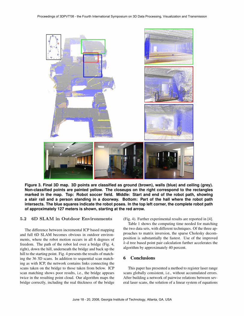
Figure 3. Final 3D map. 3D points are classified as ground (brown), walls (blue) and ceiling (grey).Non-classified points are painted yellow. The closeups on the right correspond to the rectanglesmarked in the map. Top: Robot soccer field. Middle: Start and end of the robot path, showinga stair rail and a person standing in a doorway. Bottom: Part of the hall where the robot pathintersects. The blue squares indicate the robot poses. In the top left corner, the complete robot pathof approximately 127 meters is shown, starting at the red arrow.

5.2 6D SLAM in Outdoor Environments

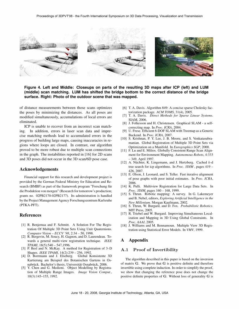
The difference between incremental ICP based mappingand full 6D SLAM becomes obvious in outdoor environ-ments, where the robot motion occurs in all 6 degrees offreedom. The path of the robot led over a bridge (Fig. 4,right), down the hill, underneath the bridge and back up thehill to the starting point. Fig. 4 presents the results of match-ing the 36 3D scans. In addition to sequential scan match-ing as with ICP, the network contains links connecting thescans taken on the bridge to those taken from below. ICPscan matching shows poor results, i.e., the bridge appearstwice in the resulting point cloud. Our algorithm maps thebridge correctly, including the real thickness of the bridge

(Fig. 4). Further experimental results are reported in [4].Table 1 shows the computing time needed for matching

the two data sets, with different techniques. Of the three ap-proaches to matrix inversion, the sparse Cholesky decom-position is substantially the fastest. Use of the improvedk-d tree based point pair calculation further accelerates thealgorithm by approximately 40 percent.

6 Conclusions

This paper has presented a method to register laser rangescans globally consistent, i.e., without accumulated errors.After building a network of pairwise relations between sev-eral laser scans, the solution of a linear system of equations

Proceedings of 3DPVT'08 - the Fourth International Symposium on 3D Data Processing, Visualization and Transmission

June 18 - 20, 2008, Georgia Institute of Technology, Atlanta, GA, USA

Figure 4. Left and Middle: Closeups on parts of the resulting 3D maps after ICP (left) and LUM(middle) scan matching. LUM has shifted the bridge bottom to the correct distance of the bridgesurface. Right: Photo of the outdoor scene that was mapped.

of distance measurements between those scans optimizesthe poses by minimizing the distances. As all poses aremodified simultaneously, accumulations of local errors areeliminated.

ICP is unable to recover from an incorrect scan match-ing. In addition, errors in laser scan data and impre-cise matching methods lead to accumulated errors in theprogress of building large maps, causing inaccuracies in re-gions where loops are closed. In contrast, our algorithmproved to be more robust due to multiple scan connectionsin the graph. The instabilities reported in [16] for 2D scansand 3D poses did not occur in the 3D scan/6D pose case.

AcknowledgementsFinancial support for this research and development project is

provided by the German Federal Ministry for Education and Re-search (BMBF) as part of the framework program ”Forschung furdie Produktion von morgen” (Research for tomorrow’s production;grants no. 02PB2170-02PB2177). Its administration is handledby the Project Management Agency Forschungszentrum Karlsruhe(PTKA-PFT).

References

[1] R. Benjemaa and F. Schmitt. A Solution For The Regis-tration Of Multiple 3D Point Sets Using Unit Quaternions.Computer Vision – ECCV ’98, 2:34 – 50, 1998.

[2] R. Bergevin, M. Soucy, H. Gagnon, and D. Laurendeau. To-wards a general multi-view registration technique. IEEETPAMI, 18(5):540 – 547,1996.

[3] P. Besl and N. McKay. A method for Registration of 3–DShapes. IEEE TPAMI, 14(2):239 – 256, 1992.

[4] D. Borrmann and J. Elseberg. Global Konsistente 3DKartierung am Beispiel des Botanischen Gartens in Os-nabruck. Bachelor’s thesis, Universitat Osnabruck, 2006.

[5] Y. Chen and G. Medioni. Object Modelling by Registra-tion of Multiple Range Images. Image Vision Comput.,10(3):145–155, 1992.

[6] T. A. Davis. Algorithm 849: A concise sparse Cholesky fac-torization package. ACM TOMS, 31(4), 2005.

[7] T. A. Davis. Direct Methods for Sparse Linear Systems.SIAM, 2006.

[8] J. Folkesson and H. Christensen. Graphical SLAM - a self-correcting map. In Proc. ICRA, 2004.

[9] U. Frese. Efficient 6-DOF SLAM with Treemap as a GenericBackend. In Proc. ICRA, 2007.

[10] S. Krishnan, P. Y. Lee, J. B. Moore, and S. Venkatasubra-manian. Global Registration of Multiple 3D Point Sets viaOptimization on a Manifold. In Eurographics SGP, 2000.

[11] F. Lu and E. Milios. Globally Consistent Range Scan Align-ment for Environment Mapping. Autonomous Robots, 4:333– 349, April 1997.

[12] A. Nuchter, K. Lingemann, and J. Hertzberg. Cached k-dtree search for icp algorithms. In Proc. 3DIM , pages 419 –426, 2007.

[13] E. Olson, J. Leonard, and S. Teller. Fast iterative alignmentof pose graphs with poor initial estimates. In Proc. ICRA,2006.

[14] K. Pulli. Multiview Registration for Large Data Sets. InProc. 3DIM, pages 160 – 168, 1999.

[15] S. Thrun. Robotic mapping: A survey. In G. Lakemeyerand B. Nebel, editors, Exploring Artificial Intelligence in theNew Millenium. Morgan Kaufmann, 2002.

[16] S. Thrun, W. Burgard, and D. Fox. Probabilistic Robotics.MIT Press, 2005.

[17] R. Triebel and W. Burgard. Improving Simultaneous Local-ization and Mapping in 3D Using Global Constraints. InProc. AAAI, 2005.

[18] J. Williams and M. Bennamoun. Multiple View 3D Regis-tration using Statistical Error Models. In VMV, 1999.

A Appendix

A.1 Proof of Invertibility

The algorithm described in this paper is based on the inversionof matrix G. We prove that G is positive definite and thereforeinvertible using complete induction. In order to simplify the proof,we show that changing the reference pose does not change thepositive definite properties of G. Without loss of generality G is

Proceedings of 3DPVT'08 - the Fourth International Symposium on 3D Data Processing, Visualization and Transmission

June 18 - 20, 2008, Georgia Institute of Technology, Atlanta, GA, USA

a positive definite matrix of the form (3), (4), with the referencenode X0. Switching the reference node to Xi results in the matrixG′. These two matrices are related by

G′ = IiG

where Ii is an identity matrix of size (dn × dn) with a row ofnegative (d× d) identity matrices of the form:

Ii =

0@ Id(i−1) 0 0−Id . . . −Id

0 0 Id(n−i+1)

1A .

Multiplication with Ii corresponds to replacing the submatrices at(i, j) with the negative sum of all submatrices at row j. Since Iiis invertible, G′ remains positive definite.

Induction base k = n Assuming a graph with n + 1 nodesand n links. The matrix G is transformed into the block diagonalmatrix G′, composed of covariance matrices by

G′ = IDGITD,

with an upper-right triangular matrix ID of d-dimensional identitymatrices

ID =

0B@ Id . . . Id

. . ....

0 Id

1CA .

Since G′ is given by

G′i,i = C−1

i−1,i

G′i,j = 0 (i 6= j)

and all covariances are positive definite, G′ itself is positive defi-nite. The same holds for G, as ID is invertible.

Inductive step k → k + 1 Let G be a positive definite ma-trix that corresponds to a graph with n + 1 nodes and k links.An additional link between the nodes Xi and Xj is inserted, withpositive definite covariance Ci,j . Without restriction, Xi is thereference node of the given graph, since the reference pose is ar-bitrary. Thus, the resulting matrix G′ is changed only at the d× dsubmatrix G′

j,j:

G′j,j = Gj,j + C−1

i,j .

In case Ci,j is positive definite, G′∗ is positive definite, too, iff

XT G′X > 0 X ∈ Rd·n X 6= 0,

which is equivalent to

nXk,l=1

XTk G′

k,lXl > 0, (14)

where Xk are the d-dimensional subvectors of X. ExpandingEq. (14) to

nXk,l=1

XTk G′

k,lXl = XTj G′

j,jXj +

nXk,l=1

k 6=l6=j

XTk Gk,lXl

= XTj C−1

i,j Xj +

nXk,l=1

XTk Gk,lXl

= XTj C−1

i,j Xj + XT GX > 0.

G′ is a positive definite matrix. �

A.2 Fast construction of the linear equa-tion system

To solve the linear equation system GX = B,

C−1D = (MT M)/s2 and C−1

D D = (MT Z)/s2

are needed. To calculate these efficiently, summations are sub-stituted for matrix multiplication by using the regularities in thematrix M. MT M is represented as a sum over all correspondingpoint pairs: MT M =

mXk=1

0BBBBBB@1 0 0 0 −yk −zk

0 1 0 zk xk 00 0 1 −yk 0 xk

0 zk −yk y2k + z2

k xkzk −xkyk

−yk xk 0 xkzk y2k + x2

k ykzk

−zk 0 xk −xkyk ykzk x2k + z2

k

1CCCCCCA .

Similarly, MT Z is calculated as follows:

MT Z =

mXk=0

0BBBBBB@∆xk

∆yk

∆zk

−zk ·∆yk + yk ·∆zk

−yk ·∆xk + xk ·∆yk

zk ·∆xk − xk ·∆zk

1CCCCCCAwith 0@ ∆xk

∆yk

∆zk

1A = Zk = Va ⊕ uak − Vb ⊕ ub

k

and an approximation for each point:0@ xk

yk

zk

1A = uk ≈`Va ⊕ ua

k + Vb ⊕ ubk

´/2.

Finally s2 is a simple summation using the observation of the lin-earized measurement equation D = (MT M)−1MT Z:

s2 =mP

k=0

`∆xk − (D0 − yk · D4 + zk · D5)

´2

+`∆yk − (D1 − zk · D3 + xk · D4)

´2

+`∆zk − (D2 + yk · D3 − xk · D5)

´2.

Di denotes the i-th entry of the vector D. Summation of C−1D and

C−1D D yields B and G.

Proceedings of 3DPVT'08 - the Fourth International Symposium on 3D Data Processing, Visualization and Transmission

June 18 - 20, 2008, Georgia Institute of Technology, Atlanta, GA, USA