The Effect of Bank Capital Requirements on Bank Loans Rates

Jonathan Wallen1

March, 12, 2017

Abstract

A large literature discusses the effects of bank capital requirements on lending. The contribution

of this paper is to empirically quantify this effect on the cost of bank credit. On average, banks

increased tier one capital ratios by 4 percent from 2008 through 2011. This increase in bank

capital raised the cost of borrowing by 20 basis points. I identify this effect using heterogeneity

in the timing of banks raising capital. To address endogeneity concerns, I deploy various cuts of

the data, control groups, differences in risk weights, and an instrument for changes in bank

capital. These various identification approaches consistently estimate that for each percentage

point increase in bank capital, bank loan rates increase by approximately 5 basis points.

1 I thank Arvind Krishnamurthy for advising me throughout this paper. I thank Anat Admati, Svetlana Bryzgalova,

John Cochrane, Darrell Duffie, Hanno Lustig, Amit Seru, and Victoria Vanasco for helpful conversations and

comments.

The usual disclaimer applies.

Email: jwallen@stanford.edu. Address: Knight Management Center, 655 Knight Way, Stanford, CA 94305.

I. Introduction

Financial regulators are developing increasingly sophisticated tools to promote financial

stability. At the core of these methods is capital regulation of financial intermediaries. Basel III,

through the Supplementary Leverage Ratio, requires that all US banks maintain a minimum

capital ratio of 3 percent and 5 percent for globally systematically important banks.2 The

implementation of capital requirements following the recent financial crisis is mired by a

longstanding debate associated with the costs of bank capital requirements. In an open letter to

the Financial Times, twenty professors argued in favor of higher bank capital requirements. The

letter highlights the social benefits of a healthier banking system: reduced probability of financial

crises. Of note is reference to common banking rebuttals: “equity requirements would restrict

lending and impede growth.”3 This debate is at the forefront of proposed policy changes to the

Dodd–Frank Wall Street Reform and Consumer Protection Act.4 The contribution of this paper is

to quantify the effect of bank capital requirements on the cost of credit.

Discussing the costliness of equity capitalization implies greater funding costs for banks

with more equity. Such a change in funding costs deviates from Modigliani and Miller (1958)

(MM). A common such deviation is through the tax subsidy of debt. Kashyap, Stein, and Hanson

(2010) add taxes to the model of MM and find that the frictions of raising capital are likely to be

more expensive than the present value of higher capital ratios. In addition to any tax benefits,

Kelly, Lustig, and Van Nieuwerburgh (2016) find that government guarantees subsidized bank

equity holders by $282 billion dollars over the financial crisis. Such government guarantee of

bank debt similarly breaks MM and raises the costs of equity capital. These types of deviations

from MM are due to distortionary transfers, which Admati et al. (2013) cover in depth. In

contrast, suppose that banks have a technological advantage to issuing debt. A plausible such

technological advantage may be in the funding advantage of deposits (Diamond and Rajan,

2001). Gornall and Strebulaev (2015) find supply chain effects which lower credit costs of

highly leveraged banks. Bank technological advantages to issuing debt deviates from MM in a

manner that generates socially costly equity capital for banks. I am agnostic about the reason

equity is a more expensive source of capital for banks. To contribute to this debate, I quantify the

effect of bank capital requirements on loan pricing. By measuring pass-through effects on loans,

I identify an economy-wide effect of bank capital requirements.

To empirically quantify this, I measure the change in bank credit pricing following an

increase in reported tier one capital. On aggregate, tier one capital for US banks increased from a

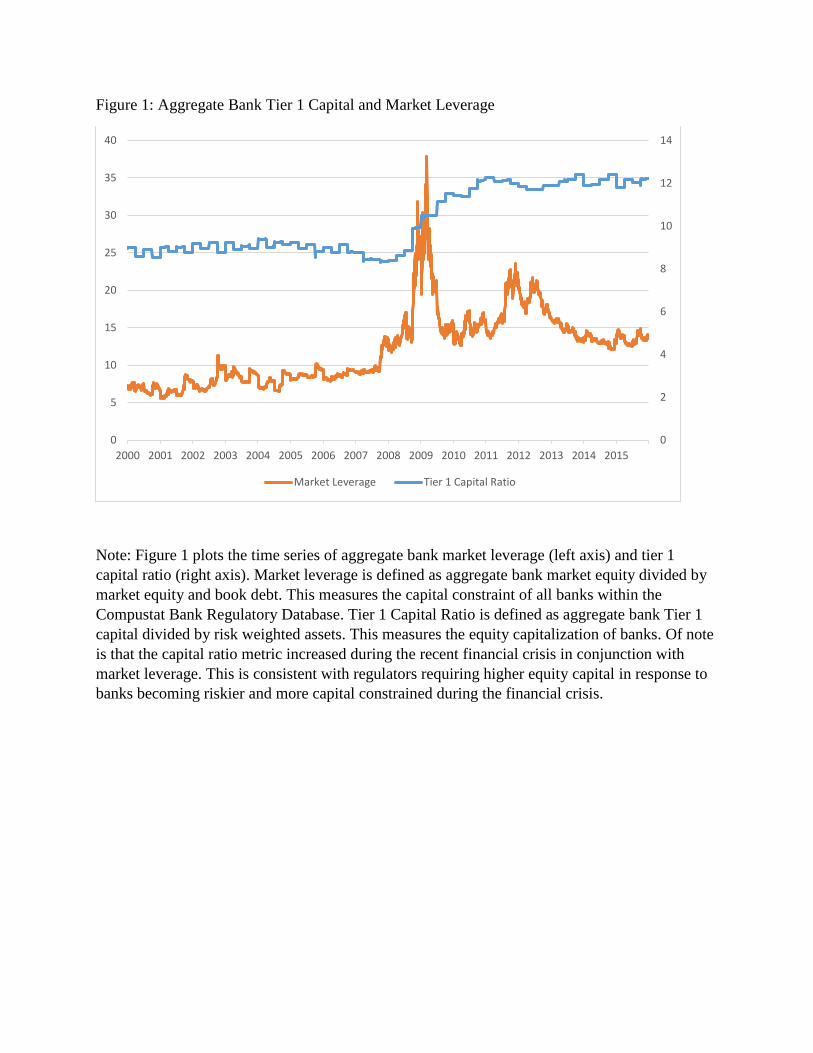
steady 8.5 percent prior to the financial crisis to 12 percent (see Figure 1). This change occurred

heterogeneously in magnitude and timing. Deleveraging of banks happened at the behest of

financial regulators. Both theory and practitioners document that bank leverage increases

shareholder value. Admati et al. (2016) describe from contracting theory the Leverage Ratchet

Effect, where shareholders prefer greater leverage. From a practitioner’s perspective, financial

2 Basel Committee on Banking Supervision (2014) 3 Admati et al. (2010) 4 On February 3, 2017, the President of the United States signed an executive order outlining, “Core Principles for

Regulating the United States Financial System.”

markets primarily value banks based on return on equity. Begenau and Stafford (2017) find

about 70 percent of the cross-sectional variation in bank valuation multiples may be explained by

ROE. Banks with high ROE due to high leverage receive high market valuations.

Using heterogeneity in raising tier 1 capital requirements, I find that bank loans costs

increased by 20 basis points. As capital regulations were slowly implemented following the

recent financial crisis, tier one capital ratios increased from 8.5 to 12 percent. For each unit of

increased capital, syndicated loan spreads increased by about 5 basis points. These findings are

robust to controls for macroeconomic conditions, firm characteristics, year fixed effects, and

time invariant borrower industry unobservables. These estimates are broadly consistent with

theoretical models, which calibrate the increased cost of bank capital. Baker and Wurgler (2015)

use empirical data on the low-risk anomaly5 to estimate an 8.5 basis point effect per percentage

point of additional bank equity capital. From a standard MM model with taxes, Kashyap, Stein,

and Hanson (2010) estimate about a 3.5 basis point effect per percent of additional bank capital.

Despite a battery of controls identification concerns persist. To confirm the direction of

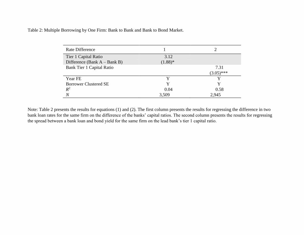
the effect, I use the cleanest cut of the data: firms with multiple debt issuances. In a Kwaja and

Mian (2008) style, I subsample to firms that borrow from more than one bank and firms that

borrow from both a bank and the bond market. I find that the difference in borrowing rates is

positively associated with the difference in bank capital. For a firm that borrows from two banks

within a year, credit from the bank with more capital is costlier. Similarly, the spread between a

bank loan and bond yield for a firm is positively associated with the bank’s capital. In effect, I

find that greater bank capital requirements increase the cost of bank credit.

To assess the robustness of the magnitude of the effect of capital requirements on bank

credit, I use the bond market as a control group. Changes to aggregate bank capital may effect

both bond and bank markets. For example, banks underwrite and intermediate bond issuances.

However, bank capital requirements do not directly impact the funding costs of investors. I

estimate an incremental effect of bank capital requirements on the cost of bank credit, relative to

bond issuances. An additional percent of bank capital incrementally increases the cost of bank

credit by 5 basis points.

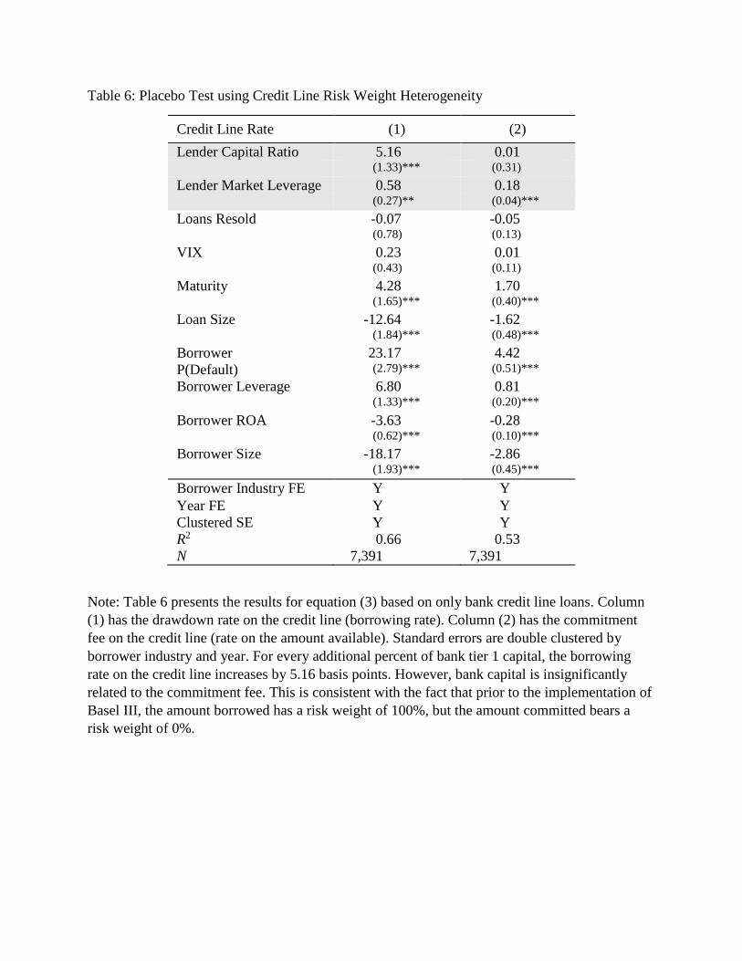
To verify the bank capital requirements channel, I perform a placebo test using the

pricing of bank credit lines. Credit lines are commitments by banks to lend a maximum amount

on specified terms: maturity, rate, and commitment fee.6 Prior to the implementation of Basel III,

the unused portion of credit lines had a risk weighting of 0%. The used portion of credit lines,

similar to all corporate loans, bore 100% risk weight. For the same lending contract, the bank

prices a capital requirement sensitive component and an unsensitive component. The pricing of

credit line commitment fees should be unrelated to bank capital requirements. However, the

borrowing rate on credit lines should be positively related to bank capital requirements. Using

the subsample of syndicated credit line loans, I verify the placebo test. Credit line commitment

5 Empirical evidence by Ang et al. (2006) documents a low-risk anomaly: realized cost of equity is higher for less

risky firms. 6 Sufi (2009) provides an empirical characterization of credit line covenants and how firms use credit lines.

fees do not vary with bank capital requirements, while the borrowing rate increases by 5 basis

points for each additional percentage point of tier one capital.

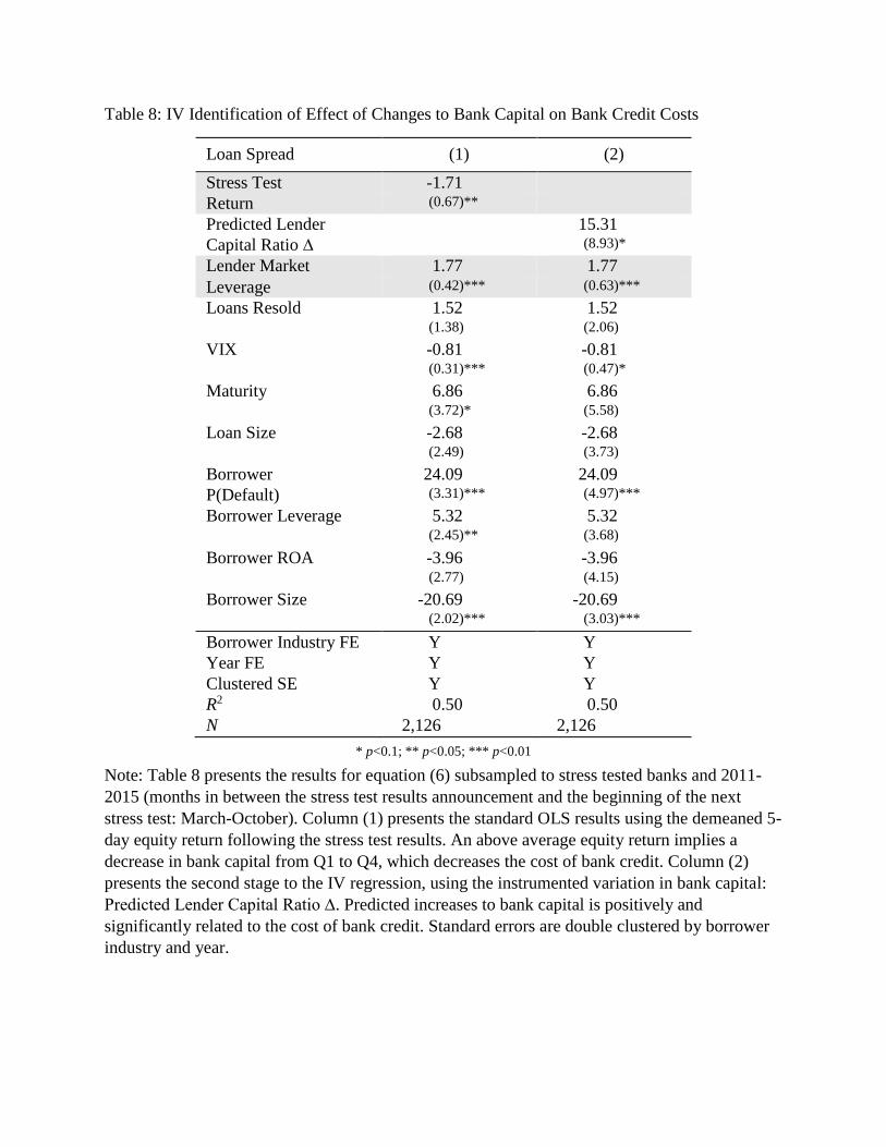
As a final robustness check, I instrument for changes to bank capital. Bank equity returns

over the Federal Reverse’s announcement of stress test results from 2011 to 2015 predict

changes to bank tier one capital. The relevance of the variable is evident from the purpose of the

stress test: assess whether banks have sufficient capital (DFAST, 2016). However, there are

endogeneity concerns about market return of banks following the stress test results. Investors and

banks may learn about credit market conditions through the stress test. Negative equity returns

may reflect worsening credit risk, which would motivate banks to raise capital and increase loan

rates. To address this concern, I demean the market equity return of banks following the stress

test results. Consequently, I am identifying only on the heterogeneity of bank stress test results.

Any endogeneity concern must line up with the particular ordering of bank equity returns

following the stress test. This instrumented variation in bank capital yields slightly larger

estimated effects. A predicted increase of one percent of tier one capital increased syndicated

loans spread by 15 basis points. Part of this larger effect may be transitory. Banks that performed

most poorly in the stress test may be pushing to decrease their risk weighted assets before the

next stress test.

Interpreting these effects depends on whether bank equity capital is expensive due to

distortionary transfers or technological advantages to issuing debt. Suppose that it is due to

distortionary incentives for debt capital, then interpret the effect as a decrease in bank borrowing

subsidies. However, if banks add value by issuing debt, then these 20 basis points represent a

social welfare cost to bank capital regulation. Although small, this credit cost applies to all bank

loans: 235 billion dollars of consumer loans and 1,870 billion dollars of commercial and

industrial loans.7

II. Bank Capital Requirements

First, I document the heterogeneity of timing and magnitude by which bank capital

requirements propagated through banks. I characterize this heterogeneity as driven by regulatory

enforcement. Due to subjective stress test metrics and different risk exposures, banks differed in

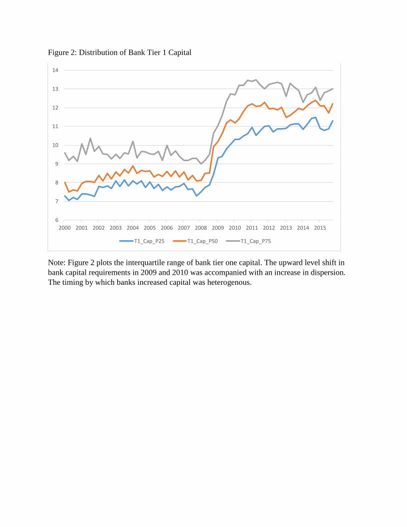
their recapitalization. Figure 2 illustrates the distribution of tier one capital: the level increases

and distribution widens following the financial crisis. This variation in the time series and cross

section of bank capital ratios is crucial for identifying an effect on the cost of bank credit.

Bank capital ratios increased during the financial crisis, implying a safer banking system.

However, measures of bank stress peaked. Figure 1 portrays a puzzling positive relationship with

bank capital reserves and market leverage. When banks have more book equity relative to risk

weighted assets, banks also have less market equity relative to assets. He, Kelly and Manela

(2016) show that innovations to a market measure of bank capital prices the cross section of asset

returns. In short, the market leverage of banks matters for asset risk premia. This is consistent

with the characterization of market leverage as a measure of the capital constraint of financial

intermediaries. The mechanism for this is through the pricing of corporate default swaps. Short

7 Consumer loan and commercial and industrial loan data from Federal Reserve Bank of St Louis as of Fall 2016.

term bank debt is a combination of a risk-free asset with a small sliver of bank equity.8 In effect,

bank credit risk is primarily priced based on variation in the market value of bank equity.

However, the primary regulatory measure for bank reserves is positively correlated with the

market measure of bank capital scarcity.

To resolve this tension, interpret market leverage as a measure of bank risk and changes

to aggregate bank tier one capital reserves to reflect greater regulatory requirements. Safe banks

may have both low market leverage and high tier one capital ratios in levels. Aggregate bank

capital reserves increased from 8 percent of risk weighted assets prior to the financial crisis of

2008 to 12 percent in 2010. This reflected more regulatory pressure, not a healthier banking

system. New banking regulation expanded the discretionary enforcement of bank capital.

The increased enforcement of bank capital requirements included both strict rules and

qualitative judgement. Under Basel III, banks are required to have a minimum capital ratio of

4.5% of risk weighted assets with an additional 1%-3.5% for systemically important financial

institutions.9 Complementing these explicit requirements, regulators use discretion in

maintaining financial stability. The primary example of the Federal Reserve’s discretionary

enforcement of capital reserves is the stress test. Through the DFAST (Dodd Frank-Act Stress

Test), the federal reserve assesses the ability of banks to maintain sufficient capital reserves

under a variety of adverse economic conditions. A core purpose of this assessment is to ensure

that banks “continue lending to support real economic activity, even under adverse economic

conditions.”10 For the smaller banks, the FDIC regulators similarly use hard rules and judgement.

Goldsmith-Pinkham et al. (2016) use computational linguistics to study how regulators use both

discretionary qualitative and quantitative information in regulating banks. The addition of

discretionary enforcement of a buffer of capital explains why all banks do not have the minimum

amount of capital.

Variation in bank capital reflects regulatory enforcement. Abnormal bank equity returns

following the announcement of stress test results predict changes to bank capital ratios. A bank’s

tier one capital ratio increases by 11 basis points for each 1% below average return. This effect is

unique to market returns following the announcement of stress test results. There is no effect of

market returns one month prior and after the stress test on bank capital.11 Regulatory action and

negative market returns jointly predict increased tier one capital reserves. Although unsurprising,

these results highlight regulatory scrutiny as a determining factor of bank capital reserves.

III. Data

Despite the lack of a US credit registry, Retuers Loan Pricing corporation provides data

on bank loans derived from SEC filings. This DealScan dataset primarily includes larger,

syndicated bank loans. These syndicated loans are between one borrower and a group of lenders.

The lead lender negotiates the loan terms for the group. From the DealScan dataset, I construct a

8 Consistent with this channel, Hilscher, Pollet, Wilson (2015) find that equity returns lead credit default returns. 9 Basel III (2010) 10 DFAST (2013) 11 See Table 7 as described in the Empirical Identification and Results section.

panel of lead lender and borrower pairs with the associated loan pricing terms. The matching of

loan data to firm and lender data follows the standard established by Chava and Roberts (2008)

and Schwert (2016). I expand the matching to lenders in Schwert (2016) to include all bank

holding companies regulated by the Federal Reserve. Complementing the DealScan dataset on

bank loans, I use Thompson Reuter’s SDC Platinum for data on bond market issuances of the

firms.

Through variation in lead lender’s tier one capital ratio and market leverage, I identify

supply side effects on loan pricing. Lender and firm balance sheet and market leverage

information are from Compustat and CRSP. Additionally, I use probability of default data to

measure firm credit risk; the data is sourced from the Singapore Risk Management Institute’s

CRI database. Following Botsch and Vanasco (2016), I measure the loan borrowing rate as the

all-in drawn spread over LIBOR and exclude non-standard loans.12 For the credit line pricing

placebo test, I use DealScan data on the pricing of facility fees: all-un drawn spread. Credit lines

typically include a borrowing rate for the portion utilized and a fee on the portion unutilized.

Berg, Saunders, and Steffen (2015) extensively describe the complex details of loan pricing.

Although the DealScan dataset begins coverage in 1981, data is exceptionally sparse until the

late 1990’s. Many of the identification approaches depend on sufficient variation in bank tier one

capital ratios and firms having borrowed from multiple lead lenders. Consequently, I limit the

sample to loans initiated after 2000 through 2015. Table 1 presents summary statistics of the

data.

IV. Empirical Identification and Results

The primary contribution of this paper is to document an effect of capital requirement on

the pricing of bank credit. A large literature theoretically models the effect of capital

requirements on bank cost of capital. I focus on the real economic effect of greater bank capital

requirements on the cost of bank credit. The pass-through of bank capital cost changes to lending

may reflect a variety of market frictions and features. To identify this effect, I employ a variety

of methods with various cuts of the data.

i. One Firm and Two Banks & One Firm, a Bank Loan, and a Bond Issuance

Using the cleanest cut of the data, I establish that greater bank capital requirements

increase the cost of bank credit. This directional evidence follows from two subsamples of the

data: firms that borrow from more than one bank and firms that borrow from both a bank and the

bond market. This identification style is similar to Kwaja and Mian (2008); I use initial loan

pricing rather than a time series of volumes. I regress the difference in the borrowing rate of bank

loans on the difference in the bank tier one capital ratios. Formally, the specification is

𝑅𝑎𝑡𝑒𝑖,𝑎,𝑡 − 𝑅𝑎𝑡𝑒𝑖,𝑏,𝜏 = 𝛼 + 𝛾𝑡 + 𝛽 (𝐶𝑎𝑝𝑎,𝑡 − 𝐶𝑎𝑝𝑏,𝑡) + 𝜖𝑖,𝑡 (1)

where 𝑅𝑎𝑡𝑒𝑖,𝑎,𝑡 is the bank loan rate for borrower 𝑖, lead bank 𝑎, made at time 𝑡. The

second loan has a 𝑅𝑎𝑡𝑒𝑖,𝑏,𝜏 for the same borrower 𝑖, different lead bank 𝑏, made at time 𝜏, where

12 I include syndicated loans reported as “term loans,” “364-day facilities,” or “revolving lines of credit.”

|𝜏 − 𝑡| ≤ 365 days. I control for time trends using time fixed effects, 𝛾𝑡. The sole explanatory

variable of interest is (𝐶𝑎𝑝𝑎,𝑡 − 𝐶𝑎𝑝𝑏,𝑡), the difference between bank 𝑎’s and bank 𝑏′𝑠 capital

ratios. Standard errors are clustered at the borrower level. This identification nets out any

borrower characteristics and identifies an association between bank capital and loan rates.

Similarly, for the bank to bond comparison, I regress the difference in the bank rate less the bond

rate on the bank lender’s tier one capital ratio.

𝑅𝑎𝑡𝑒𝑖,𝑏𝑎𝑛𝑘,𝑡 − 𝑅𝑎𝑡𝑒𝑖,𝑏𝑜𝑛𝑑,𝜏 = 𝛼 + 𝛾𝑡,𝐵𝑜𝑛𝑑 + 𝛾𝑡,𝐵𝑎𝑛𝑘 + 𝛽 𝐶𝑎𝑝𝑏𝑎𝑛𝑘,𝑡 + 𝜖𝑖,𝑡 (2)

This specification also nets of borrower characteristics, while highlighting the relationship

between the bank-bond spread and bank capital. Note that I include separate time fixed effects

for the bond market and bank credit, which allows the two markets to have different time trends.

Higher bank capital requirements is associated with higher bank loan rates relative to

both other bank loans and bonds. Table 2 presents the results. One firm that borrows from two

different banks within a year pays more for the loan from the bank with a higher tier one capital

ratio. The difference is an additional 3.12 basis points for each percentage point difference in

bank capital. Bank borrowing rates are on average about 3% cheaper than bond yields. However,

this spread narrows when banks have more capital. For a firm borrowing from both markets

within a year, the bank loan becomes relatively more expensive when banks report higher tier

one capital ratios. Bank credit costs increase by 7.31 basis points relative to public credit for each

additional percentage point of bank capital.

ii. Full Sample with Controls

Complementing the subsample of multi-borrowing firms, I estimate the effect of greater

capital requirements on the full sample. In doing so, I comprehensively control for borrower

characteristics and present several robust cuts of the bank loan data.

Without differencing out borrower characteristics, the primary identification challenge

relates to borrower riskiness and demand for bank credit. For borrower riskiness, I include

borrower 4 digit SIC industry fixed effects to capture time invariant unobservable characteristics.

To control for time varying characteristics, I control for borrower probability of default. Default

probability is estimated from a distance to default measure (volatility adjusted book leverage).13

Duffie, Saita, and Wang (2007) document that distance to default explains a substantial portion

of the term structure of conditional future corporate default probabilities. I use the firm’s market

leverage to supplement the book measure of default probability. I include borrower profitability

to measure demand for bank credit. Kothari, Lewellen, and Warner (2015) document that firm

investment increases primarily in response to high profits and stock returns, not interest rates.

Additionally, I control for borrower size as a rough proxy of the firm’s bargaining power relative

to the bank.

To rule out potential confounding effects, I include a set of time series controls. I use

time fixed effects to capture trends in the cost of bank credit. To control for individual bank

13 I am grateful to the National University of Singapore, Risk Management Institute for making their Credit

Research Initiative Database available.

credit risk, I use market leverage: market equity and book debt all divided by market equity. I

control for the Chicago Board Options Exchange Volatility Index (VIX) to capture broad

financial market risk aversion and uncertainty. Bekaert, Hoerova, and Duca (2013) decompose

the VIX into two components: investor risk taking appetite and expected stock market

volatility.14 Similarly, I control for volume in the secondary market for bank loans. As more

loans are resold, banks are increasingly intermediating credit. If demand for loans in the

secondary market is high, banks may act as credit intermediaries and pass on lower credit

spreads. Other channels by which this may impact loan prices are partially ruled out by

Benmelech, Dlugosz, and Ivashina (2012). They find that this securitization does not suffer from

large adverse selection effects. Other controls include loan-specific features such as maturity and

size.

Given these controls, I assess the effect of bank capital requirements on loan pricing. I

hypothesize that the cost of bank credit increases with bank capital requirements. Formally, the

specification is

𝑅𝑎𝑡𝑒𝑖,𝑙,𝑡 = 𝛼𝑖 + 𝛾𝑡 + 𝛽1𝐶𝑎𝑝𝑙,𝑡 + 𝜉𝑋𝑖,𝑡 + 𝜖𝑖,𝑙,𝑡 (3)

where 𝑅𝑎𝑡𝑒𝑖,𝑙,𝑡 is the yield spread on a loan for borrower 𝑖, lead bank 𝑙 and time 𝑡 against

LIBOR. 𝐶𝑎𝑝𝑙,𝑡 is the tier one capital ratio of the lead bank in the syndicate. Controls, 𝑋𝑖,𝑡, are

discussed in detail above. Standard errors are double clustered by four digit SIC industry and

time, following Petersen (2009). Clustering by industry is particularly apt because bank loans

prices may be heuristically benchmarked against a firm’s industry comparables.

For each additional percentage point of capital, bank credit costs increased by 5 basis

points. From 2008 to 2011, aggregate bank capital increased from 8% to 12%, corresponding to a

increase in bank credit costs of 20 basis points. Table 3 presents these findings. Column (1) does

not include borrower industry or time fixed effects. Column (2) includes borrower industry and

year fixed effects to capture unobservable differences among industries and time trends in the

bank credit market. Column (4) includes the controls and fixed effects. The coefficients on the

control variables are robustly in the expected direction. Borrower riskiness metrics (probability

of default and leverage) are associated with higher spreads. Larger and more profitable firms

with more valuable earnings (Size and ROA) borrow at lower rates.

Across all specifications, I find a positive and significant coefficient on bank capital. The

magnitude of the coefficient is smallest, but most robust, when I estimate over variation limited

to within industry and year. Firms borrowing from lenders that have implemented higher equity

capital requirements pay more for loans. These firms borrow at an additional 5.16 basis points

for each additional percent of bank capital. However, for the market measure of bank risk, I find

a consistent positive coefficient. Riskier lenders with higher market leverage charge more for

loans. This negative coefficient on reported leverage and positive coefficient on market leverage

is consistent with a supply shock characterization of bank capital requirements. The

14 Becker and Ivashina (2014) develop a measure for bank credit supply scarcity as the proportion of firms

borrowing from banks relative to those that borrow form banks or the bond market in a given quarter. I consider this

control, but later find that it is subsumed by year fixed effects.

implementation of regulatory capital requirements reflects in changes to bank capital. Market

leverage measures the riskiness of a bank.

This effect of bank capital requirements appears to be heterogeneous among firm quality.

Firms with low five-year probability of default are less effected than risky firms. Table 4 cuts the

dataset into two sets of firms: those with a five-year default probability below 0.5% and those

above 5%. For the low risk firms, I find a positive, but small and statistically insignificant effect

of bank capital requirements on bank credit costs (Column 1). However, high risk firms

experienced an even greater increase to bank credit costs in association with bank capital

requirements. Column (2) documents an increase of 6.73 basis points for each unit of additional

bank capital. The economic explanations for this differential are many. Financial regulation may

have more so disciplined risky, rather than safe, bank lending. Banks may be more able to

offload safe loans with low information asymmetry. This finding is consistent with a large,

significant negative effect of loan resale on borrowing rates of the low risk group, but

insignificant effect on the risky group. However, this explanation is at odds with Drucker and

Puri (2009) who find that all else equal banks offload riskier debt.15 Begenau, Piazzesi, and

Schneider (2015) characterize bank risk exposures and shed light on methods to estimate off-

balance sheet exposures. There is interesting future work to be done in this area.

iii. Bank Credit Costs vs Bond Market Yields

I estimate the incremental effect of lender-specific capital regulation on bank credit

relative to bond issuances. Changes to bank capital requirements may have spillover effects or

coincide with other changes to credit markets. Besides these aggregate effects, bank capital

regulation directly impacted bank funding costs, but not bond market investors. This incremental

estimate is robust to any confounding factors that are not specific to bank credit.

The effect of capital regulation has a direct impact on bank loans, but not for bond

issuances. In the latter, investors bear the credit risk on their balance sheets. Investors balance

sheets are not directly impacted by greater bank capital requirements. I hypothesize that the

interaction effect between a bank loan dummy and bank capital increases borrowing costs. This

tests the incremental effect of bank capital on bank credit costs relative to bond yields:

𝑅𝑎𝑡𝑒𝑖,𝑙,𝑡 = 𝛼𝑖 + 𝛾𝑡 + 𝛽1𝐶𝑎𝑝𝑙,𝑡 + 𝛽2𝐵𝑎𝑛𝑘 𝐿𝑜𝑎𝑛 ∗ 𝐶𝑎𝑝𝑙,𝑡 + 𝜉𝑋𝑖,𝑡 + 𝜖𝑖,𝑙,𝑡 (4)

This identification allows for bank capital regulation to have an aggregate effect on credit. A

market microstructure example of such a channel is the intermediation of banks in the bond

issuance process. In the sample, 24% of firms borrow from both the bond market and banks.

Using this variation, I estimate an incremental effect of bank capital requirements on the cost of

bank credit.

Relative to bond yields, the incremental effect of an additional percent of bank capital on

bank credit costs is 5.36 basis points. Table 5 documents a robust positive coefficient on the

interaction of a bank loan dummy and bank capital. The most robust specification: Column (3)

15 Future work includes assessing whether this may have changed in the recent years. Drucker and Puri (2009) study

the period of May 1998 to September 2005.

includes controls, time trends for both bank and bond markets, and borrower fixed effects. Of

note is that bank loans tend to be on average cheaper by 3%. The effect of bank capital

requirements and riskiness is positively, but insignificantly related to aggregate credit costs.

However, the two are incrementally significantly increasing the cost of bank credit. I include

Column (1) with only the bank supply variables and loan dummy to highlight that these variables

explain 34% of the variation in borrowing rates. With all of the controls, the specification

(equation 4, Column (3)) explains 83% of the variation in borrowing rates.

iv. Credit Line Placebo Test

Prior to the implementation of Basel III, credit lines contained features with 0% risk

weight and 100% risk weight.16 A credit line is a commitment of a lender to make available

funds to a borrower on demand. The contract stipulates a borrowing rate for the portion of the

credit line used and an interest rate on the unused portion (commitment fee). For bank capital

requirements, the utilized portion of credit lines bear a 100% risk weight, while the unused

portion has 0% risk weight. The pricing of the borrowing rate depends on bank capital

requirements. A drawdown on a credit line increases the risk weighted assets of the bank,

requiring the bank to raise capital to maintain its tier one capital ratio. However, committing to

make available additional capital upon demand is an off-balance sheet exposure. This does not

change the banks regulatory risk weighted assets or capital ratio. I hypothesize that the

borrowing rate for bank credit lines depends on bank capital requirements, but the commitment

fee does not. The latter serves as a placebo test. If variation in bank capital also explains the

pricing of the 0% risk weight portion of credit lines, a confounding effect is at hand.

Credit line borrowing rates increase by 5.16 basis points with each additional percent of

bank capital requirements, while commitment fees do not. Table 6 presents the results. Following

equation (3), I subsample to only include bank credit lines prior to 2014 (precludes Basel III).

Column (1) presents the results with the borrowing rate on the left hand side. Higher capital

requirements increase bank credit costs and riskier banks charge more for credit. Column (2) has

the commitment fee on the left hand side. Riskier banks charge more for committing to make

funds available, but bank capital requirements have no statistically significant effect. This

placebo test rules out potential confounding effects or omitted variables that may generate a

spurious relationship between bank capital and credit costs.

v. Stress Test Instrument

Discretionary features in bank regulation generates variation in bank capital. The most

prominent of these is the Federal Reserve’s stress test of banks. The relative performance of

banks in the stress test predicts changes to bank capital ratios. From 2001-2015, the Federal

Reserve published stress test results for the banks in March. Using equity returns in the week

following announcement, I predict changes to bank capital ratios as reported in the Federal

16 Basel III increased the risk weight on bank credit lines with an original maturity greater than 1 year to 50%. See

the FDIC RC-R Regulatory Capital general instructions section. The implementation of Basel III happened slowly

and banks began voicing concerns about the proposed new risk weight on credit lines in 2014. See J.P. Morgan’s

February 2014 report “Corporate finance with a sprig of Basel.”

Reserve call reports from Q1 to Q4. The Call Report data on bank balance sheets is available for

Q1 at the time of the stress test announcement. Since the subsequent stress test begins in

November-December, the relevant comparison call report is the one reported in Q4. Formally,

the first stage is

𝐶𝑎𝑝𝑙,𝑄4,𝑡 − 𝐶𝑎𝑝𝑙,𝑄1,𝑡 = 𝛼 + 𝛽1𝑅𝑒𝑡𝑙,𝑡 + 𝜖𝑙,𝑡 (5)

where 𝐶𝑎𝑝𝑙,𝑄4,𝑡 is bank 𝑙’s tier one capital ratio as reported in Q4 of stress test year 𝑡. 𝑅𝑒𝑡𝑙,𝑡 is

the demeaned market equity return of bank 𝑙 in the 5 trading days following the stress test

announcement.

Table 7 documents that an abnormal 1 percent equity decline following the stress test

announcement predicts an increase in bank capital of about 11 basis points (Column 1). This

instrument has sufficiently strong power: F-statistic 15.25. The relationship between equity

returns following the stress test and changes to bank capital is robust to year and bank fixed

effects (Columns 2 and 3). Furthermore, as a placebo test, I consider 5-day bank equity returns

30 days before the stress test (Column 4) and 30 days after (Column 5). The coefficients on

bank equity returns outside of the stress test results announcement are close to zero and

statistically insignificant.

The instrument is both relevant and exogenous. The primary purpose to the stress test is

to assess whether banks have sufficient capital following an adverse macroeconomic scenario.

The performance of banks in the Federal Reserve’s stress tests is directly relevant for their

capital structure. In terms of the exogeneity requirement, there is a concern about learning. The

stress test may reveal information about credit market conditions to investors and banks.

Worsening credit risk would result in both negative equity returns and higher capital buffers. To

address this concern, I demean the market equity return of banks. Consequently, I am identifying

only on the heterogeneity of bank stress test results. Any endogenous effect would need to line

up with the particular ordering of bank equity returns following the stress test results.

Using the predicted change to bank capital, I estimate the effect on bank credit costs in

the window between this year stress test results and the beginning of next year’s stress test. The

specification replaces bank capital with instrumented bank capital (𝐶𝑎𝑝𝑙,𝑡 ) in equation (3):

𝑅𝑎𝑡𝑒𝑖,𝑙,𝑡 = 𝛼𝑖 + 𝛾𝑡 + 𝛽1𝐶𝑎𝑝𝑙,𝑡

+ 𝜉𝑋𝑖,𝑡 + 𝜖𝑖,𝑙,𝑡 (6)

Table 8 presents the results. A predicted increase to bank capital of 1 percent raises bank

credit costs by 15.31 basis points. Column (1) shows the OLS results of using bank equity

returns following the stress test results. As expected, worse performance on the stress test implies

higher bank credit costs. The channel is through bank capital reserves. Column (2) presents the

effect of instrumented changes to bank capital on the cost of bank credit. The effect is larger, but

not statistically different from previously estimated effects using the level of bank capital ratios.

Part of this larger magnitude may be transitory. Bank credit may be especially expensive for

banks seeking to shrink their risk weighted assets before the next stress test.

V. Conclusion

A large literature discusses bank capital requirements and its effect on bank lending. The

contribution of this paper is to quantify such a causal effect. Following the financial crisis, banks

raised tier one capital from 8% of risk weighted assets in 2008 to 12% in 2011. This increase in

capital occurred through greater regulatory pressures. Both quantitative and discretionary rule

changes raised the capital requirements for banks. In particular, performance in the Federal

Reserve stress test predicts subsequent changes to bank capital. An abnormal negative return of

1% following the announcement of stress test results predicts an increase in bank capital of 11

basis points. Using the heterogeneity in the timing of banks’ raising tier one capital, I identify the

effect on bank loan rates. To address potential endogeneity concerns, I use various cuts of the

data, control groups, differences in risk weights, and an instrument for changes in bank capital.

From these identification approaches, I consistently estimate that for each percentage point

increase in bank capital, bank loan rates increase by 5 basis points.

Such a credit supply shock due to banks changing their funding composition from debt to

equity implies a violation of Modigliani and Miller (1958). Understanding the nature of this

violation is essential for interpreting the 20 basis point effect. If this is due to a distortionary

transfer, such as the tax shield or implied government guarantee of debt, capital regulations are

removing a bank loan subsidy. No effect on social welfare. A policy that subsidizes bank loans

would perfectly negate the credit supply shock effect of bank regulation, leaving the benefit of a

better capitalized banking system. However, if bank cost of capital increased due a technological

advantage of banks issuing debt, social welfare is lost. The dollar cost is 20 basis points for all

bank debt. Scaled by 235 billion consumer and 1,870 billion commercial and industrial bank

loans, 20 basis points are economically significant. These findings highlight the importance of

understanding economic mechanism behind why bank credit costs increased due to capital

regulation.

References

Admati, Anat et al. 2010. “Healthy banking system is the goal, not profitable banks.” Financial

Times [open letter].

Admati, Anat, Peter Demarzo, Martin Hellwig, Paul Pfleiderer. 2013. “Fallacies, Irrelevant

Facts, and Myths in the Discussion of Capital Regulation: Why Bank Equity is Not

Expensive.” Stanford GSB Working Paper No. 2065

Admati, Anat, Peter Demarzo, Martin Hellwig, Paul Pfleiderer. 2016. “The Leverage Ratchet

Effect.” Stanford GSB Working Paper No. 3029

Ang, Andrew, Robert Hodrick, Yuhang Xing, and Xiaoyan Zhang. 2006. “The Cross-Section of

Volatility and Expected Returns.” Journal of Finance 61 (1): 259–99.

Baker, Malcolm, and Jeffrey Wurgler. 2015. "Do strict capital requirements raise the cost of

capital? Bank regulation, capital structure, and the low-risk anomaly." The American

Economic Review 105.5: 315-320.

Basel Committee on Banking Supervision, 2010. Basel III: A Global Regulatory Framework for

More Resilient Banks and Banking Systems, December (revised June 2011), Bank for

International Settlements, Basel, pp. 1–69.

Basel Committee on Banking Supervision, 2014. Basel III Leverage Ratio Framework and

Disclosure Requirements, January, Bank for International Settlements, Basel, pp. 1–19.

Bekaert, Geert, Marie Hoerova, and Marco Lo Duca. 2013. "Risk, uncertainty and monetary

policy." Journal of Monetary Economics 60.7: 771-788.

Becker, Bo, and Victoria Ivashina. 2014. "Cyclicality of credit supply: Firm level evidence."

Journal of Monetary Economics 62: 76-93.

Begenau, Juliane, and Erik Stafford. 2017. “Inefficient Banking.” Working Paper.

Begenau, Juliane, Monika Piazzesi, and Martin Schneider. 2015. “Banks' risk exposures.” No.

w21334. National Bureau of Economic Research.

Berg, Tobias, Anthony Saunders, and Sascha Steffen. (2015). "The total cost of corporate

borrowing in the loan market: Don't ignore the fees." The Journal of Finance.

Benmelech, Efraim, Jennifer Dlugosz, and Victoria Ivashina. 2012. "Securitization without

adverse selection: The case of CLOs." Journal of Financial Economics 106.1: 91-113.

Botsch, Matthew, and Victoria Vanasco. 2016. “Still Learning After All These Years:

Information Acquisition in Banking.” Stanford GSB Working Paper No. 3239.

Chava, Sudheer, and Michael R. Roberts. 2008. "How does financing impact investment? The

role of debt covenants." The Journal of Finance 63.5: 2085-2121.

Diamond, Douglas W., and Raghuram G. Rajan. 2001. "Liquidity risk, liquidity creation, and

financial fragility: A theory of banking." Journal of political Economy 109.2: 287-327.

DFAST. 2016. Dodd-Frank Act Stress Test 2016: Supervisory Stress Test Methodology and

Results. Federal Reserve.

Drucker, Steven, and Manju Puri. 2009. "On loan sales, loan contracting, and lending

relationships." Review of Financial Studies 22.7: 2835-2872.

Duffie, Darrell, Leandro Saita, and Ke Wang. 2007. "Multi-period corporate default prediction

with stochastic covariates." Journal of Financial Economics 83.3: 635-665.

Goldsmith-Pinkham, Paul, Beverly Hirtle, and David O. Lucca. 2016. "Parsing the content of

bank supervision." Working Paper.

Gornall, Will, and Ilya A. Strebulaev. 2015. "The economic impact of venture capital: Evidence

from public companies."

He, Zhiguo, Bryan Kelly, and Asaf Manela. 2016. “Intermediary asset pricing: New evidence

from many asset classes.” NBER Working Paper No. w21920.

Hilscher, Jens, Joshua M. Pollet, and Mungo Wilson. 2015. "Are credit default swaps a

sideshow? Evidence that information flows from equity to CDS markets." Journal of

Financial and Quantitative Analysis 50.03: 543-567.

Kelly, Bryan, Hanno Lustig, and Stijn Van Nieuwerburgh. "Too-systemic-to-fail: What option

markets imply about sector-wide government guarantees." The American Economic

Review 106.6 (2016): 1278-1319.

Kashyap, Anil K., Jeremy C. Stein, and Samuel Hanson. 2010. "An analysis of the impact of

‘substantially heightened’ capital requirements on large financial institutions." Booth

School of Business, University of Chicago, mimeo 2.

Khwaja, Asim Ijaz, and Atif Mian. "Tracing the impact of bank liquidity shocks: Evidence from

an emerging market." The American Economic Review 98.4 (2008): 1413-1442.

Kisin, Roni, and Asaf Manela. 2016. "The shadow cost of bank capital requirements." Review of

Financial Studies.

Kothari, S. P., Jonathan Lewellen, and Jerold B. Warner. 2014. "The behavior of aggregate

corporate investment." MIT working paper 5112-14.

Modigliani, Franco, and Merton H. Miller. 1958. "The cost of capital, corporation finance and

the theory of investment." The American Economic Review 48.3: 261-297.

National University of Singapore, Risk Management Institute, CRI database. Available at:

http://rmicri.org [Accessed September 13, 2016]

Petersen, Mitchell A. "Estimating standard errors in finance panel data sets: Comparing

approaches." Review of financial studies 22.1 (2009): 435-480.

Schwert, Michael. 2016. “Bank Capital and Lending Relationships.” Ohio State University

working paper.

Sufi, Amir. "Bank lines of credit in corporate finance: An empirical analysis." Review of

Financial Studies 22.3 (2009): 1057-1088.

Figure 1: Aggregate Bank Tier 1 Capital and Market Leverage

Note: Figure 1 plots the time series of aggregate bank market leverage (left axis) and tier 1

capital ratio (right axis). Market leverage is defined as aggregate bank market equity divided by

market equity and book debt. This measures the capital constraint of all banks within the

Compustat Bank Regulatory Database. Tier 1 Capital Ratio is defined as aggregate bank Tier 1

capital divided by risk weighted assets. This measures the equity capitalization of banks. Of note

is that the capital ratio metric increased during the recent financial crisis in conjunction with

market leverage. This is consistent with regulators requiring higher equity capital in response to

banks becoming riskier and more capital constrained during the financial crisis.

0

2

4

6

8

10

12

14

0

5

10

15

20

25

30

35

40

2000 2001 2002 2003 2004 2005 2006 2007 2008 2009 2010 2011 2012 2013 2014 2015

Market Leverage Tier 1 Capital Ratio

Figure 2: Distribution of Bank Tier 1 Capital

Note: Figure 2 plots the interquartile range of bank tier one capital. The upward level shift in

bank capital requirements in 2009 and 2010 was accompanied with an increase in dispersion.

The timing by which banks increased capital was heterogenous.

6

7

8

9

10

11

12

13

14

2000 2001 2002 2003 2004 2005 2006 2007 2008 2009 2010 2011 2012 2013 2014 2015

T1_Cap_P25 T1_Cap_P50 T1_Cap_P75

Table 1: Summary Statistics

Variable Mean Median Max Min St Dev Skew Kurtosis Obs

Interest Rate Spread 280.56 250.00 913.56 20.00 181.04 1.01 3.89 60905

Aggregate Bank Capital Ratio 10.16 9.22 12.40 8.28 1.52 0.34 1.26 62712

Lead Lender Capital Ratio 9.92 8.80 20.50 4.94 2.28 0.69 2.58 45856

Bank Loan Dummy 0.86 1.00 1.00 0.00 0.35 -2.08 5.31 62712

Aggregate Market Leverage 11.63 9.62 32.36 5.65 4.46 0.97 3.90 62712

Lead Lender Market Leverage 12.45 9.94 69.40 3.48 8.47 2.75 13.83 50511

Loan Resold 3.60 2.87 15.04 0.26 3.02 1.55 5.82 62712

VIX 19.62 17.71 80.86 9.89 7.79 2.03 10.32 62712

Maturity 4.81 4.75 101.47 0.08 4.80 5.09 45.06 60760

Loan Size 4.81 4.91 10.80 -2.59 1.53 -0.34 3.16 62712

Borrower Probability of

Default

0.20 0.25 4.56 -6.91 1.12 -0.14 3.69 22173

Borrower Leverage 2.85 1.87 28.68 1.04 3.49 4.99 32.39 29273

Borrower ROA 0.79 0.94 8.87 -18.51 2.93 -2.87 19.08 29133

Borrower Size 8.31 8.26 15.11 0.31 2.21 0.06 2.78 29308

Note: Interest Rate Spread is the bank or bond rate less 12-month LIBOR (DealScan and SDC). Aggregate Bank Capital Raito is the

average tier 1 capital ratio (∑ 𝑇𝑖𝑒𝑟 1 𝐶𝑎𝑝𝑖𝑡𝑎𝑙𝑛

𝑖=1

∑ 𝑅𝑖𝑠𝑘 𝑊𝑒𝑖𝑔ℎ𝑡𝑒𝑑 𝐴𝑠𝑠𝑒𝑡𝑠𝑛𝑖=1

) for all bank holding companies reported in the quarterly Commercial Bank

Database, from the Federal Reserve Bank of Chicago. Lead Lender Capital Ratio is the tier one capital ratio for the lead bank in the

syndicate of lenders. Bank Loan Dummy is a dummy variable equal to 1 if the observation is a bank loan and 0 if the observation is a

bond issuance. Aggregate market leverage is ∑ 𝑀𝑎𝑟𝑘𝑒𝑡 𝐸𝑞𝑢𝑖𝑡𝑦𝑖+𝐵𝑜𝑜𝑘 𝐷𝑒𝑏𝑡𝑖

𝑛𝑖=1

∑ 𝑀𝑎𝑟𝑘𝑒𝑡 𝐸𝑞𝑢𝑖𝑡𝑦𝑖𝑛𝑖

from Federal Reserve Call Report data (Commercial Bank

Database). Lead Lender Market Leverage is the market leverage of the lead bank in the syndicate of lenders. Loan resale is the amount

of collateralized loan obligations packaged and sold to the market as reported by Bloomberg divided by the total notional of loans

within the DealScan at a quarterly frequency. The ratio is small in part because the DealScan bank loan contracts include credit lines,

where the loan notional is the maximum available to be borrowed. VIX is the CBOE volatility index. Maturity is the years to maturity

for the debt contracts. Loan size is the natural log of the notional of the debt contract in millions. Borrower probability of default is the

borrower’s 5 year probability of default (CRI database). Borrower Leverage is the market leverage of the borrower (Compustat and

CRSP data). Borrower ROA is the return on assets of the borrower in percent (Compustat). Borrower size is the natural log of the

borrower’s total assets in millions (Compustat).

Table 2: Multiple Borrowing by One Firm: Bank to Bank and Bank to Bond Market.

Rate Difference 1 2

Tier 1 Capital Ratio 3.12

Difference (Bank A – Bank B) (1.88)*

Bank Tier 1 Capital Ratio 7.31

(3.05)***

Year FE Y Y

Borrower Clustered SE Y Y

R2 0.04 0.58

N 3,509 2,945

Note: Table 2 presents the results for equations (1) and (2). The first column presents the results for regressing the difference in two

bank loan rates for the same firm on the difference of the banks’ capital ratios. The second column presents the results for regressing

the spread between a bank loan and bond yield for the same firm on the lead bank’s tier 1 capital ratio.

Table 3: Bank Loan Identification of Capital Requirement Effect on Bank Credit Costs

Bank Loan Spread 1 2 3

Lender Capital Ratio 10.93 8.36 5.16

(1.26)*** (2.66)*** (1.25)***

Lender Market Leverage 2.75 1.36 1.36

(0.42)*** (0.28)*** (0.38)***

Loans Resold -0.53

(0.49)

VIX 0.26

(0.54)

Maturity 6.67

(1.25)***

Loan Size -6.84

(1.92)***

Borrower 25.82

P(Default) (2.35)***

Borrower Leverage 7.39

(1.09)***

Borrower ROA -4.16

(0.62)***

Borrower Size -21.92

(1.48)***

Borrower Industry FE N Y Y

Year FE N Y Y

Clustered SE Y Y Y

R2 0.08 0.18 0.55

N 45,856 18,556 12,445

* p<0.1; ** p<0.05; *** p<0.01

Note: Table 3 presents the results for equation (3). Column (1) controls for lender riskiness

(market leverage). Column (2) adds 4-digit SIC borrower fixed effects and year fixed effects.

Column (3) adds control variables for broad debt market conditions (loans resold, VIX), loan

characteristics (maturity, size), and borrower characteristics (probability to default, market

leverage, return on assets, and log total assets). Standard errors are double clustered by borrower

industry and year. Robustly across all specifications, greater bank capital requirements are

positively and significantly related to bank credit costs.

Table 4: Differential Effect of Capital Requirements on Loan Spreads by Borrower Riskiness

Bank Loan Spread 1 2

Lender Capital Ratio 2.01 6.73

(3.81) (2.05)***

Lender Market Leverage 1.92 0.21

(0.65)*** (0.79)

Loans Resold -0.58 1.56

(0.19)*** (1.86)

VIX -0.31 1.61

(0.40) (0.90)*

Maturity 3.37 5.82

(1.04)*** (3.63)

Loan Size -4.53 -7.00

(3.69) (4.77)

Borrower -2.40 29.05

P(Default) (5.48) (14.80)*

Borrower Leverage 36.58 3.86

(9.08)*** (1.43)***

Borrower ROA -3.74 -3.04

(1.56)** (1.64)*

Borrower Size -22.75 -17.92

(3.17)*** (4.48)***

Borrower Industry FE Y Y

Year FE Y Y

Clustered SE Y Y

R2 0.55 0.62

N 2,130 1,141

Note: Table 4 presents the results for equation (3) based on two subsamples: safe and risky firms.

Safe firms have a five-year probability of default of less than or equal to 0.5 percent. Risky firms

are more than 5 percent likely to default in the next five years. Columns 1 and 2 displays the

results for the safe firms and risky firms, respectively. Standard errors are double clustered by

borrower industry and year. There is substantial heterogeneity in the effect of bank capital

regulation of bank loan spreads. Risky firms experience larger loan spreads increases with high

bank capital compared to safe firms.

Table 5: Bank Loan and Bond Issuance Identification of an Incremental Capital Requirement

Effect on Loan Spreads

Loan Spread 1 2 3

Aggregate Bank Capital -17.25 14.72 15.01

Ratio (5.15)*** (13.71) (14.31)

Lender Capital Ratio * 18.71 8.75 5.36

Bank Loan Dummy (2.64)*** (1.99)*** (1.24)***

Bank Loan Dummy -496.87 -324.18 -304.42

(46.04)*** (22.67)*** (17.06)***

Aggregate Bank Market 2.04 2.38 1.66

Leverage (2.17) (2.02) (2.34)

Lender Market Leverage * 2.53 1.18 1.37

Bank Loan Dummy (0.48)*** (0.34)*** (0.39)***

Loans Resold -0.22

(0.82)

VIX 0.11

(0.47)

Maturity 5.89

(0.65)***

Loan Size 2.53

(2.80)

Borrower 28.74

P(Default) (2.54)***

Borrower Leverage 8.85

(1.35)***

Borrower ROA -4.72

(0.65)***

Borrower Size -30.66

(2.86)***

Borrower Industry FE N Y Y

Year*Bank Loan FE N Y Y

Year*Bond Issuance FE N Y Y

Clustered SE Y Y Y

R2 0.34 0.68 0.83

N 52,827 25,527 18,860

* p<0.1; ** p<0.05; *** p<0.01

Note: Table 5 presents the results for equation (4). Column 1 controls for credit supply side

effects (lender capital and riskiness, dummy for bank loan). Column 2 includes 4-digit SIC

borrower fixed effects and time fixed effects interacted with bank loan and bond issuance

(different trends in bank loan and bond markets). Standard errors are double clustered by

borrower industry and year. The interaction of lead lender capital and bank loan is robustly,

significantly positively related to borrowing spreads to LIBOR. When banks are required to hold

more equity capital bank loans become incrementally more expensive than bond issuances.

Table 6: Placebo Test using Credit Line Risk Weight Heterogeneity

Credit Line Rate (1) (2)

Lender Capital Ratio 5.16 0.01

(1.33)*** (0.31)

Lender Market Leverage 0.58 0.18

(0.27)** (0.04)***

Loans Resold -0.07 -0.05

(0.78) (0.13)

VIX 0.23 0.01

(0.43) (0.11)

Maturity 4.28 1.70

(1.65)*** (0.40)***

Loan Size -12.64 -1.62

(1.84)*** (0.48)***

Borrower 23.17 4.42

P(Default) (2.79)*** (0.51)***

Borrower Leverage 6.80 0.81

(1.33)*** (0.20)***

Borrower ROA -3.63 -0.28

(0.62)*** (0.10)***

Borrower Size -18.17 -2.86

(1.93)*** (0.45)***

Borrower Industry FE Y Y

Year FE Y Y

Clustered SE Y Y

R2 0.66 0.53

N 7,391 7,391

Note: Table 6 presents the results for equation (3) based on only bank credit line loans. Column

(1) has the drawdown rate on the credit line (borrowing rate). Column (2) has the commitment

fee on the credit line (rate on the amount available). Standard errors are double clustered by

borrower industry and year. For every additional percent of bank tier 1 capital, the borrowing

rate on the credit line increases by 5.16 basis points. However, bank capital is insignificantly

related to the commitment fee. This is consistent with the fact that prior to the implementation of

Basel III, the amount borrowed has a risk weight of 100%, but the amount committed bears a

risk weight of 0%.

Table 7: Stress Test Equity Returns Instrument: Predicting Changes to Bank Capital Ratios

Capital Ratio

Change

(1) (2) (3) (4) (5)

Stress Test -11.19 -11.08 -11.77 -1.24 0.60

Return (2.87)*** (3.11)*** (3.19)*** (3.03) (4.01)

Year FE N Y Y N N

Bank FE N N Y N N

F-Statistic 15.25 5.16 4.12 1.50 0.02

R2 0.07 0.11 0.28 0.00 0.00

N 102 102 102 102 102

* p<0.1; ** p<0.05; *** p<0.01

Note: Table 7 presents the results for equation (5). Column (1) shows the regression of Q1-Q4

changes in bank capital ratios on demeaned 5 day equity returns following the announcement of

stress test results (2011-2015). The sample covers only stress tested banks that lend to firms in

the DealScan database. Column (2) includes year fixed effects and Column (3) includes year and

bank fixed effects. Robustly across all three specifications, a 1 percent higher than average

equity return following the stress test results predicts a decreases in bank capital of 11 basis

points. Columns (4) and (5) presents the results using equity returns 30 days prior and after the

stress test results, respectively. Note that non-stress test equity returns do not predict changes to

bank tier 1 capital. Standard errors are heteroskedasticity robust.

Table 8: IV Identification of Effect of Changes to Bank Capital on Bank Credit Costs

Loan Spread (1) (2)

Stress Test -1.71

Return (0.67)**

Predicted Lender 15.31

Capital Ratio ∆ (8.93)*

Lender Market 1.77 1.77

Leverage (0.42)*** (0.63)***

Loans Resold 1.52 1.52

(1.38) (2.06)

VIX -0.81 -0.81

(0.31)*** (0.47)*

Maturity 6.86 6.86

(3.72)* (5.58)

Loan Size -2.68 -2.68

(2.49) (3.73)

Borrower 24.09 24.09

P(Default) (3.31)*** (4.97)***

Borrower Leverage 5.32 5.32

(2.45)** (3.68)

Borrower ROA -3.96 -3.96

(2.77) (4.15)

Borrower Size -20.69 -20.69

(2.02)*** (3.03)***

Borrower Industry FE Y Y

Year FE Y Y

Clustered SE Y Y

R2 0.50 0.50

N 2,126 2,126

* p<0.1; ** p<0.05; *** p<0.01

Note: Table 8 presents the results for equation (6) subsampled to stress tested banks and 2011-

2015 (months in between the stress test results announcement and the beginning of the next

stress test: March-October). Column (1) presents the standard OLS results using the demeaned 5-

day equity return following the stress test results. An above average equity return implies a

decrease in bank capital from Q1 to Q4, which decreases the cost of bank credit. Column (2)

presents the second stage to the IV regression, using the instrumented variation in bank capital:

Predicted Lender Capital Ratio ∆. Predicted increases to bank capital is positively and

significantly related to the cost of bank credit. Standard errors are double clustered by borrower

industry and year.