The effect of environmental preferences on the market for eco … · Segmentation of the market for...

Segmentation of the market for labeled ornamental plants by

environmental preferences: A latent class analysis

Nicole M. D'Alessio

Thesis submitted to the faculty of the Virginia Polytechnic Institute and State University in

partial fulfillment of the requirements for the degree of

Master of Science

In

Agricultural and Applied Economics

Kevin J. Boyle, Chair

Michael G. Sorice

Wen You

Darrell J. Bosch

May 28, 2015

Blacksburg, VA

Keywords: Latent class analysis, ornamental plants, principal component analysis, product

labeling, environmental certification, disease management, water conservation

Segmentation of the market for labeled ornamental plants by environmental preferences: A latent

class analysis

Nicole M. D'Alessio

ABSTRACT

Labeling is a product differentiation mechanism which has increased in prevalence across many

markets. This study investigated the potential for a labeling program applied in ornamental plant

sales, given key ongoing issues affecting ornamental plant producers: irrigation water use and

plant disease. Our research investigated how to better understand the market for plants certified

as disease free and/or produced using water conservation techniques through segmenting the

market by consumers‟ environmental preferences. Latent class analysis was conducted using

choice modeling survey results and respondent scores on the New Environmental Paradigm

scale. The results show that when accounting for environmental preferences, consumers can be

grouped into two market segments. Relative to each other, these segments are considered: price

sensitive and attribute sensitive. Our research also investigated market segments‟ preferences for

multiple certifying authorities. The results strongly suggest that consumers of either segment do

not have a preference for any particular certifying authority.

iii

Segmentation of the market for labeled ornamental plants by environmental preferences: A latent

class analysis

Nicole M. D'Alessio

ACKNOWLEDGEMENTS

I wish to express my sincerest gratitude to my committee chair Kevin Boyle for his invaluable

guidance, support and mentoring. I would also like to thank my committee members Michael

Sorice, Wen You and Darrell Bosch for the help they have provided me in completing my

research. This project was supported through USDA-NIFA-Specialty Crop Research Initiative

(Agreement # 2010-51181-21140).

iv

Table of Contents

List of Tables .................................................................................................................................. v

List of Figures ................................................................................................................................ vi

1. Introduction ............................................................................................................................... 1

2. Application ................................................................................................................................ 3

3. Product Labeling and Environmental Preference Literature .................................................... 5

3.1 Consumers‟ Environmental Preferences ............................................................................. 7

3.2 Demand Analysis and Market Segmentation ...................................................................... 9

4. Study Design and Administration ........................................................................................... 11

5. Economic Model ..................................................................................................................... 14

6. Results ..................................................................................................................................... 19

6.1 Respondent Characteristics ............................................................................................... 19

6.2 Principal Component Analysis ......................................................................................... 21

6.3 Segmentation Process ....................................................................................................... 22

6.4 Econometric Model Results .............................................................................................. 23

6.4.1 Testing For Preference Heterogeneity Between Certifying Authority .................... 28

7. Discussion and Conclusions ................................................................................................... 29

References ..................................................................................................................................... 32

Appendix A: Depiction of Labeling Information ......................................................................... 38

Appendix B: Choice Experiment Design ...................................................................................... 40

Appendix C: Factor Analysis Results ........................................................................................... 44

Appendix D: Latent Class Segmentation Results ......................................................................... 47

Appendix E: Example Stata Codes for Latent Class Model ......................................................... 48

Appendix F: New Environmental Paradigm Responses ............................................................... 50

Appendix G: Respondent Summary Statistics .............................................................................. 51

v

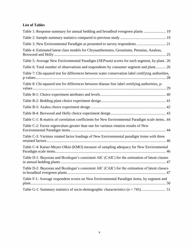
List of Tables

Table 1: Response summary for annual bedding and broadleaf evergreen plants ....................... 19

Table 2: Sample summary statistics compared to previous study ................................................ 19

Table 3: New Environmental Paradigm as presented to survey respondents ............................... 21

Table 4: Estimated latent class models for Chrysanthemums, Geraniums, Petunias, Azaleas,

Boxwood and Holly ...................................................................................................................... 25

Table 5: Average New Environmental Paradigm (NEPsum) scores for each segment, by plant . 26

Table 6: Total number of observations and respondents by consumer segment and plant ........... 26

Table 7: Chi-squared test for differences between water conservation label certifying authorities,

p-values ......................................................................................................................................... 28

Table 8: Chi-squared test for differences between disease free label certifying authorities, p-

values ............................................................................................................................................ 29

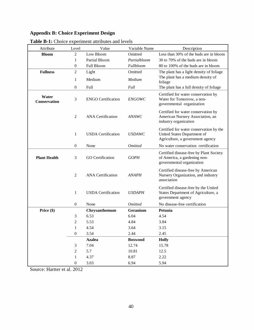
Table B-1: Choice experiment attributes and levels ..................................................................... 40

Table B-2: Bedding plant choice experiment design .................................................................... 41

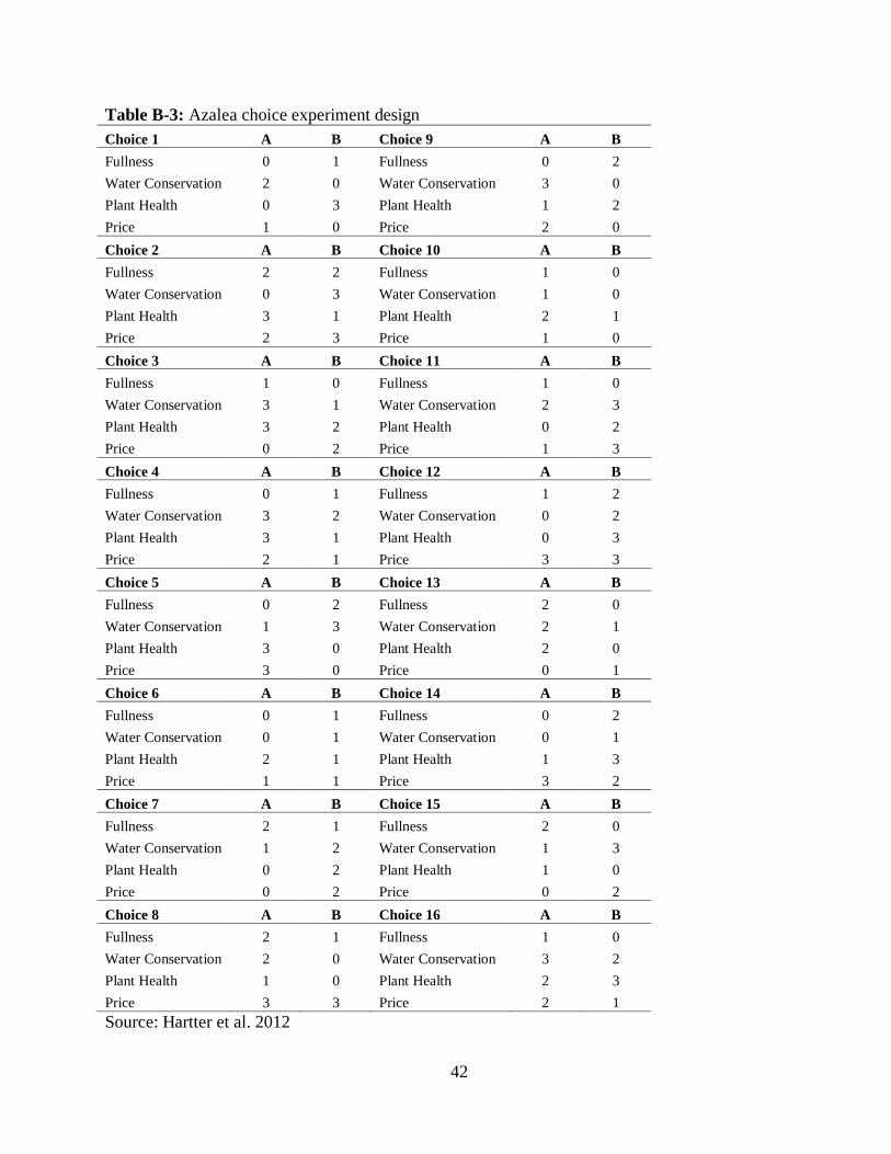
Table B-3: Azalea choice experiment design ............................................................................... 42

Table B-4: Boxwood and Holly choice experiment design .......................................................... 43

Table C-1: R-matrix of correlation coefficients for New Environmental Paradigm scale items .. 44

Table C-2: Factor eigenvalues greater than one for varimax rotation results of New

Environmental Paradigm items ..................................................................................................... 44

Table C-3: Varimax rotated factor loadings of New Environmental paradigm items with three

retained factors .............................................................................................................................. 46

Table C-4: Kaiser-Meyer-Olkin (KMO) measure of sampling adequacy for New Environmental

Paradigm scale items..................................................................................................................... 46

Table D-1: Bayesian and Bozdogan‟s consistent AIC (CAIC) for the estimation of latent classes

in annual bedding plants ............................................................................................................... 47


in broadleaf evergreen plants ........................................................................................................ 47

Table F-1: Average respondent scores on New Environmental Paradigm items, by segment and

plant............................................................................................................................................... 50

Table G-1: Summary statistics of socio-demographic characteristics (n = 745) ......................... 51

vi

List of Figures

Figure A -1: Water Conservation certification labels ................................................................... 38

Figure A-2: Disease-Free certification labels ............................................................................... 39

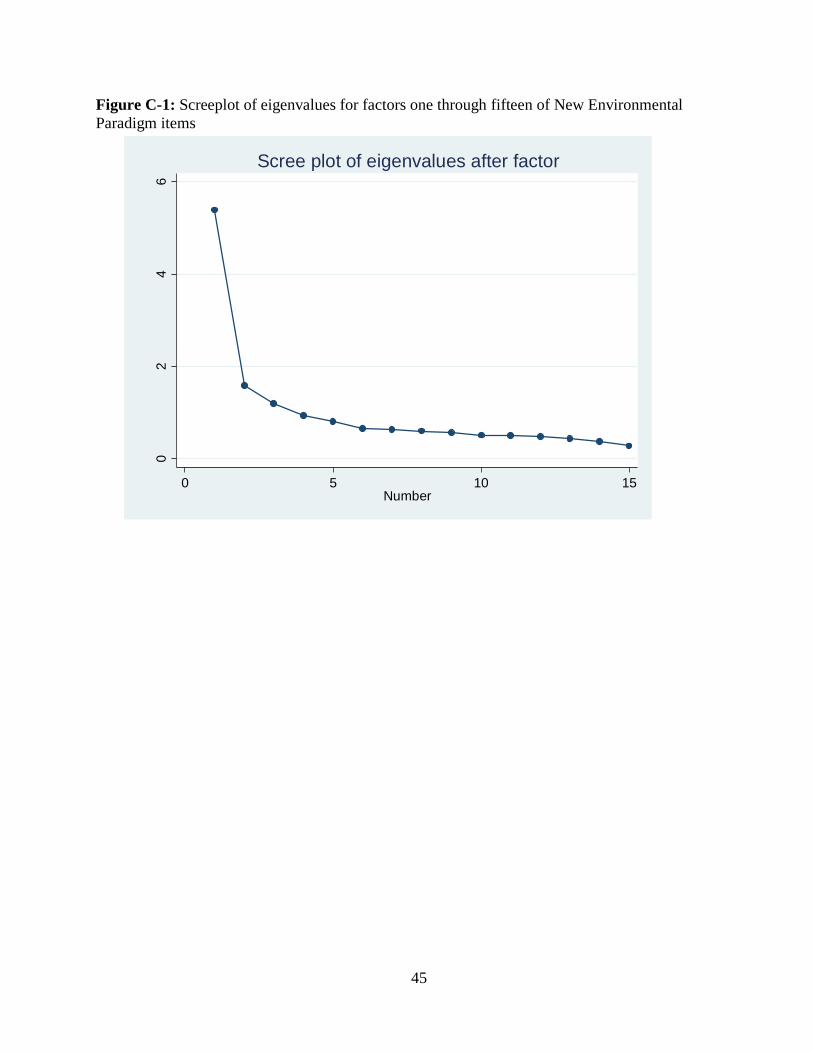
Figure C-1: Screeplot of eigenvalues for factors one through fifteen of New Environmental

Paradigm items.............................................................................................................................. 45

1

1. Introduction

Labeling as a product differentiation mechanism has increased in prevalence across many

products in recent decades, particularly among credence goods. Credence goods are

characterized by asymmetric information; a consumer is unable to observe differences among

goods with varying attributes, but nevertheless has preferences for these attributes. When

unobservable attributes are environmental in nature, such as production that utilizes less resource

intensive methods, labels can better facilitate informed purchasing decisions (Galarraga

Gallastegui 2002; Dulleck and Kerschbamer 2006; Baksi and Bose 2007). Given the availability

of two products, one being more environmentally friendly but otherwise not differentiable at the

time of sale, a label allows consumers to make tradeoffs between environmental attributes and

corresponding prices. Producers can potentially recover some of the added costs of resource-

conserving production methods by differentiating their goods through the use of labels.

Two key issues affecting ornamental plant producer profitability include availability of

irrigation water and plant disease. Drought concerns and controlling runoff have resulted in shifts

toward water conserving production practices. Capture and reuse of irrigation water has been

found to potentially result in higher incidences of disease reinnoculation of plants. Capturing

runoff to reduce nonpoint source pollution and mitigating plant disease are costly endeavors for

producers.

Certification programs are well suited to ensuring that agricultural goods are produced in a

specific manner, such as water conserving methods, or comply with specified guidelines, such as

not host to diseases. These certification schemes can be made apparent to consumers through of

labels applied to products at the time of sale. Thus, development of a certification program and

2

plant labels are one way for producers of ornamental plants to offset the cost of controlling

runoff and mitigating disease if they reuse water captured from their operations.

The focus of this paper is on investigating consumer preferences for two labeling

certification schemes for ornamental plants:

healthy plant certification, which guarantees a disease-free plant, and

water conservation certification, which ensures that a plant has been grown using

water conserving growing practices.

The specific objectives of this study are as follows:

investigate if there are significant price premiums for healthy plant and water

conservation labeled plants;

investigate if plant certifying authority affects price premiums; and

investigate heterogeneity in consumer preferences for labeled plants.

These objectives are investigated in a choice experiment conducted with purchasers of

ornamental plants; the plant labels and certifying authorities are attributes in the choice

experiment.

The results indicate plant purchasers will pay price premiums for healthy plant and water

conservation labeled plants, but the certifying authority (government, industry or NGO) does not

affect price premiums. Results also suggest that by accounting for individuals‟ environmental

preferences, we can identify two segments in the market for ornamental plants. One segment is

relatively more sensitive to price, while the second is relatively more sensitive to plant attributes.

3

These findings are useful for ornamental plant producers by allowing them to better market their

products and recoup some of the costs of evolving production practices.

2. Application

Irrigation water is the principal means by which ornamental plant producers encourage and

control plant growth, minimize losses and ensure plant hardiness (Atkinson et al. 1994). Ongoing

effects of drought have increased the risk of production loss among producers, who use large

quantities of water in production (Folger, Cody and Carter 2013).1 For example, within the

contiguous United States, 56% of land area faced moderate to exceptional drought in January

2015 (The National Drought Mitigation Center 2015). Conservation methods to reduce the risk

associated with water availability such as irrigation water recapture and recycling are costly to

implement. Therefore, if producers are to offset some of the costs of recapturing it is necessary to

develop a mechanism to command price premiums. These price premiums could be obtained by

a labeled certification program that guarantees production in accordance with water

conservation.

Many geographic areas have been experiencing water quality degradation due to nonpoint

source pollution from agriculture. In some such areas, federal and state agencies have begun to

encourage producers to meet Total Maximum Daily Load (TMDL) nutrient loading targets by

way of capturing irrigation and stormwater runoff. The Chesapeake Bay in particular has been

subject to such TMDL targets for nitrogen and phosphorus. Many state governments have been

relying on a voluntary approach to meet nutrient loading reduction goals, while the U.S.

Environmental Protection Agency maintains the ability to take regulatory action in the future to

ensure that nutrient targets are met (Cultice et al. 2013). In Maryland, state regulatory

1 Throughout this paper, ornamental plant producers will be referred to as “producers”.

4

enforcement of management practices which reduce nutrient loading in accordance with TMDLs

has been enacted. Nurseries in particular have been highlighted as a key source from which the

mandated 24% reduction in nitrogen loading and 12% in phosphorus loading by 2025 will be

achieved in Maryland (Maryland Department of The Environment 2012). Capture and recycling

of irrigation and stormwater runoff provides a solution for producers to reduce their

susceptibility to water shortages, while also complying with TMDL goals.

Though there are benefits to producers associated with irrigation water recycling, this

practice also compromises an operation‟s resilience against water-borne plant diseases.

Recycling of runoff comes at the increased risk of reinnoculating plants with water-borne

pathogens, which have the potential to result in significant production losses. When such water-

borne diseases are present in an operation, water which is applied to infected plants and

recaptured may still contain diseases. If this water is reapplied to plants in an operation, there

exists a chance that the disease can reinfect original plants bearing the disease and also infect

additional plants throughout an operation. A 2012 survey of Mid-Atlantic ornamental plant

producers indicated that 36% of respondents experienced plant losses to disease in excess of 3%

of their sales (Rees et al. 2014). In particular, Pythium and Phytophthora have been identified as

two diseases affecting ornamentals, which have been found to re-infect plants when water is

recycled and reapplied throughout an operation (Hong and Moorman 2005; Moorman 2010a;

Moorman 2010b). Consequently, producers must take extra precautionary measures to reduce

disease reinnoculation when recycling water, which result in increased operating costs.

Faced with incentives to conserve water and reduce runoff, management practices to capture

and recycle may increase in adoption in coming years. Consequently, producers who undertake

5

these practices may expect to see increased upfront and ongoing infrastructure, operating and

maintenance-related costs in addition to possible disease management costs.

Should producers choose to adopt these costly strategies, an option to mitigate higher

production costs is to charge higher prices for plants. However, there is no reason to expect

consumers will be willing to pay higher prices unless they are able to perceive a valuable

difference in the product. Assuming consumers have a positive willingness to pay for resource-

conserving production practices, creation of healthy plant and water conservation labels which

differentiate plants produced using certain management practices could result in price premiums.

The magnitude of these price premiums would be dependent on consumer willingness to pay for

them, however any premium gained could help to offset a portion or all of the increased costs

associated with these production methods (Yue, Hurley and Anderson 2011). Labels increase the

transparency of the otherwise non-observable environmental attributes, and thereby facilitate

transfer of consumer‟ willingness to pay for goods which minimize their concerns about the

environmental impact of plant production via the price premium. Those consumers who derive

the most utility from environmental production attributes have the option to buy labeled plants

which are likely to be sold at a price premium, while those who do not share the same viewpoint

will still have the option of buying ornamental plants which don‟t bear a label at a lower price

point.

3. Product Labeling and Environmental Preference Literature

Information captured by product labels varies greatly between product types. In general,

labels exist to display information pertaining to product-specific attributes to potential

consumers, such as price, quality, nutrition, and production characteristics (Teisl and Roe 1998).

Claims and certifications presented on a label are especially useful as product differentiation

6

mechanisms for credence goods. Inclusion of product-specific labeling information reduces the

costs borne by consumers of recognizing hidden attributes while also increasing the level of trust

and transparency between consumers and producers (Thøgersen 2002; Crespi and Marette 2001;

Baksi and Bose 2007).

Labeling is a predominant means by which producers can readily present information

pertaining to unobservable environmental attributes associated with producing or consuming a

particular good (Blend and Ravenswaay 1999; Rotherham 1999; Galarraga Gallastegui 2002).

Shifting consumer preferences in favor of more ecologically-conscious goods has resulted in the

widespread adoption of many labeled products in numerous industries, including: “Dolphin

Free” tuna, Partial Zero Emissions Vehicles, and USDA Organic food products (Teisl, Roe and

Hicks 2002; Noblet, Teisl and Rubin 2006; United States Department of Agriculture National

Agricultural Statistics Service 2014).

There are a number of factors that influence a consumers‟ propensity to purchase

environmentally-related labeled goods; such as: environmental consciousness, social values,

perception of and ability to identify the highlighted environmental attributes, one‟s utilitarian

value of environmental attributes, one‟s perception of their ability to mitigate environmental

issues, and costs and availability of the labeled product (Hemmelskamp and Brockmann 1997).

Chen and Chai (2010) found that personal environmental norms contribute towards attitudes

regarding consumption of green products. James et al. (2009) found that increased knowledge of

agricultural systems resulted in a lower willingness to pay for organic and local applesauce.

These aforementioned factors are likely to vary across geographic range, culture, and product

market. As such, investigation regarding the impact of environmental preferences on

consumption of labeled products is likely to be more pertinent on a case-specific basis.

7

The demand for labeled ornamental plants has been the subject of numerous studies which

have indicated that consumers are willing to pay a price premium on products bearing such

labels. Increased utility and a willingness to pay this premium for a label have been found for:

powdery mildew resistant flowering dogwoods; Texas Earth-Kind™ and Superstar™ plants;

“origin-certified” native plants; plants grown in biodegradable containers and those that are

carbon-saving; noninvasive and native plants; privately certified eco-labeled roses and low-

carbon footprint roses; and plants grown using energy-saving production practices, sold in non-

plastic containers, and locally grown plants (Gardner et al. 2002; Klingeman et al. 2004; Collart,

Palma and Hall 2010; Curtis and Cowee 2010; Yue et al. 2010; Michaud, Llerena and Joly 2012;

Khachatryan et al. 2014). The prices that consumers are willing to pay for these goods are

reflective of their private utility derived from these aforementioned products in addition to the

societal benefits associated with the highlighted environmental attributes. Consumers‟ values

placed on societal benefits related to their product purchases are indicated by their increased

utility for labeled goods and therefore a corresponding price premium.

3.1 Consumers’ Environmental Preferences

Effective marketing of environmental attributes requires and understanding of how

environmental preferences influence consumer behavior. For voluntary and easily performed

behaviors that lend themselves to deliberation, such as the purchase of labeled ornamental plants,

the Theories of Reasoned Action and Planned Behavior are useful for predicting and explaining

the influence of attitudes and beliefs (Ajzen 1991; Sorice et al. 2011). These theories suggest that

a consumer‟s behavioral beliefs pertaining to the environment shape their attitudes into

behavioral intentions and therefore influence their final purchasing decisions (Best and Mayerl

2013).

8

Findings in behavioral psychology literature have suggested that higher levels of concern for

the environment and more ecologically-centered worldviews influence environmentally

sustainable consumption due to their effect on behavioral intentions (Kollmuss and Agyeman

2002). Behaviors which aim to limit the environmental impact of consumption have been shown

to be linked to an individual‟s environmental concern and worldview in a number of cases,

including: water conserving behavior (Gilg and Barr 2006; Willis et al. 2011; Wolters 2014);

purchase of sustainable tourism alternatives (Hedlund 2011); purchase of beverages with

environmentally friendly packaging and eco-friendly disposal methods (Birgelen, Semeijn and

Keicher 2009); energy conservation (Wicker and Becken 2013); and eco-labeled fish purchases

(Brécard et al. 2009).

Among the most commonly used indicator of environmental preferences across disciplines is

the New Environmental Paradigm (NEP) scale, which measures an individual‟s ecological

worldview; that is, their „primitive beliefs‟ pertaining to their level of concern for the

environment (Dunlap 2008). High NEP scores, which represent an ecologically-oriented

worldview, have been found to be indicative of ecologically-conscious behavior in numerous

studies (Roberts and Bacon 1997; Tarrant and Cordell 1997; Ebreo, Hershey and Vining 1999;

Kotchen and Reiling 2000; Clark, Kotchen and Moore 2003). It follows that these primitive

beliefs should also have some bearing, though not necessarily a direct linear relation, on

consumption and purchasing patterns for various environmental goods. Khachatryan (2014)

found that individuals with higher than average scores on an environmental concern scale were

willing to pay a higher price premium for Chrysanthemums produced using pro-environmental

production practices. However, the measure of support for the environment used in this study

was based on Schultz (2001) which measures egoistic, altruistic and biospheric environmental

9

concerns, not a general ecological worldview as with the NEP scale. While there may be

measures of support for the environment more directly tied to choice behaviors, NEP was used in

this study because it is a scale with established reliability and validity which has been used in

other economic applications.

In this study, respondent scores on the NEP scale were used in conjunction with preferences

for plant attributes in order to group individuals into segments. However, because there is no

consensus regarding how many constructs of worldview that NEP measures, use of the scale in

research requires identification of factors present in a specific sample. The number of dimensions

identified within the scale have varied widely in literature: three dimensions have been reported

by Albrecht et al. (1982) and Thapa (2001); Edgell and Nowell (1989) found evidence for both

unidimensionality and three dimensions between samples; Amburgey and Thoman (2012) found

five interrelated dimensions. NEP was created to be an additive, unidimensional scale with

internal consistency. Dunlap (2008) reports that there may be as few as one or many as five

underlying facets of the measures worldview depending on the sample used, but suggests factor

analysis should be conducted on a case-specific basis because the number of factors found have

varied across samples and applications. Accordingly, we employed principal component analysis

here to investigate the presence of multiple dimensions in our sample.

3.2 Demand Analysis and Market Segmentation

Understanding consumer groups is important both for initial choices about what products will

be identified by certification, and also for identifying efficient marketing strategies for likely

consumer groups (Behe et al. 2013). Should there be multiple consumer groups identified in a

market, producers and industry groups can better target their sales. Due to the fact that

ornamental plants are agricultural goods and their production generates an environmental impact,

10

it is expected that environmental beliefs are taken into account during the purchasing process.

Taking these beliefs into account can better inform our investigation of heterogeneity within the

market for labeled ornamental plants.

Segmenting the market for labeled plants is a crucial step in marketing products and in the

creation of certification programs. Characterizing segments has long since been a valuable tool in

product marketing through facilitating a firm‟s ability to cater to heterogeneous preferences of

distinguishable consumer groups, with each segment being made up of individuals with

homogenous preferences (Smith 1956; Swait 1994). Analyses of consumer segments have been

previously conducted in the ornamental plant industry based on demographic and prior

purchasing characteristics (Behe 2006; Dennis and Behe 2007; Behe and Dennis 2009; Behe et

al. 2013). Environmental preferences can be accounted for by simultaneously explaining choice

behavior and segmenting the market for ornamental plants via latent class modeling. Market

segments can be readily identified using consumer choice survey data by assessing

commonalities between respondents‟ worldviews and their choice behaviors. This framework

has recently been applied in the economic literature in a number of different areas: preference

heterogeneity for wilderness visitation characterized by individuals‟ motivations for visiting and

preferences for wilderness management (Boxall and Adamowicz 2002); an assessment of fishing

preferences for segments characterized by environmental attitudinal data (Morey, Thacher and

Breffle 2006); motivations for preservation and heterogeneity in preferences for landscape

preservation (Morey et al. 2008); and travel demand preferences as segmented by individuals‟

attitudes about conventional travel versus “greener” cities (Hurtubia et al. 2014). Specifically,

the effect of environmental preferences as measured by the New Environmental Paradigm on

market segmentation via latent class analysis for stated preference data has been used by Milon

11

and Scrogin (2006) as well as Kotchen and Reiling (2000). Research identifying segments of

ornamental plant consumers by explicitly accounting for environmental preferences has not been

performed in product labeling economics literature.

4. Study Design and Administration

For this research, consumer preferences were elicited using a choice modeling framework.

Choice modeling is commonly used for estimating consumer demand and implicit prices for

attributes or products not available in markets at the time of research. Questions and choice

scenarios included in the survey were developed with the assistance of academic horticultural

experts and expert ornamental plant producers in the industry (Hartter et al. 2012).

Focus groups were used to assess the quality of the online instrument, identify effective and

readily understood questions and also to aid in determining key attributes and their

corresponding levels in the choice experiment. Three two-session focus groups consisting of 7-9

consumers with varying degrees of gardening experience were held in Blacksburg, Richmond

and Virginia Beach, Virginia between 2011 and 2012. Following the focus groups, two online

pilot studies were employed to further test the online survey instrument and ease of timely

completion among respondents. Individuals completing the pilot studies included samples of 152

consumers expressing an interest in gardening and 350 consumers from an ornamental plant

retailer in the Washington D.C. metro area (Hartter et al. 2012).

Based on the focus groups, key attributes of importance were selected. Those attributes

chosen for choice questions included: plant species, density, color, blossoms present, whether or

not a given plant blooms and the presence of labels. Subsequent pilot studies informed

coefficient values for use in the choice set designs. Ornamental plant types were chosen due to

12

their susceptibility to water-borne diseases, in particular, Pythium and Phytophthora. Sales levels

were also used as a secondary measure to identify susceptible plants with the largest sales

volumes. Annual bedding and perennial broadleaf evergreen plants were selected for the study

due to their prevalence in the market for horticultural products. In 2009, annual bedding plant

sales amounted to $2.3 billion, or 18% of all horticultural specialty sales, while broadleaf

evergreen plant sales were $793 million, or 7% of all horticultural sales (United States

Department of Agriculture 2010). Because focus group participants identified the presence of

blossoms as an attribute that would influence their plant purchases, both blossoming bedding

plants and evergreen plants were included in the survey to allow for differences between

preferences for both plant types (Hartter et al. 2012).

The specific annual bedding plants chosen for inclusion in the final survey were: Petunia,

Geranium, and Chrysanthemum, which together comprised 20% of total national annual bedding

sales in 2009 (United States Department of Agriculture 2010). Broadleaf evergreen plants chosen

for analysis were Azalea, Boxwood and Holly, which comprised 39% of total national broadleaf

evergreen sales in 2009 (United States Department of Agriculture 2010).

The final online survey instrument included a choice experiment in which individuals were

asked to make hypothetical plant purchase decisions based key plant characteristic and labeling

attributes. The labels included for consideration by participants were water conservation labels,

certifying that plants had been produced using water conservation techniques, and plant health

labels, certifying that a plant is disease-free at the time of sale. In order to test if consumer utility

for these labels varied by certifying authority, multiple authorities were included in the choice

experiment (Hartter et al. 2012). Those included in the choice experiment were water

conservation labels and plant heath labels certified by a government authority, a non-

13

governmental organization (NGO) and an industry organization. The U.S Department of

Agriculture was selected to represent the governmental certifying authority for both water

conservation and plant health labels, while fictitious certifying authorities were employed for the

depiction of both the NGO and industry labels. These fictitious authorities were defined as: the

NGO American Nursery Association, which was applied for both label types as well as Water for

Tomorrow, which was used for water conservation labeling, and Plant Society of America,

which was used for plant health labeling (Hartter et al. 2012).

Labels were depicted for respondents as they would be presented at a retailer, both as affixed

to a plant pot and as a tag placed in soil along with price and physical attribute information. The

prices used in the choice experiment were chosen to be representative of the study area, with

retail price data observed at home and garden centers and nurseries in the area at the time of

survey construction (Hartter et al. 2012).

Respondents who had indicated that they were in the market for a specific plant, based on a

previous purchase of the plant within the preceding 12 months for annual bedding and 24 months

for broadleaf evergreen, were presented with a choice scenario pertinent to their purchasing

patterns (Hartter et al. 2012).2 For each plant that respondents were considered to be in the

market for, they were instructed to choose one of two plant options (both of the same plant type)

with varying physical, labeling and price attributes, or indicate that they would purchase neither.

The survey instructed respondents that in each choice scenario, attributes that were not explicitly

mentioned such as plant color were the same between the two plants presented.

2 Due to the method by which we identified individuals in the market for given plants, we may have missed

sampling individuals who would have joined the market given the presence of labels.

14

D-efficiency was used as the criterion for identifying choice profiles presented in the survey,

as a full-factorial design would not have been feasible (Hartter et al. 2012). By using D-

Efficiency as a design criterion, we were able to select attribute levels for each profile in a

manner which minimized the errors associated with choice question designs. Using Ngene,

sixteen profiles each were created for annuals, Azaleas, and shrubs: Holly and Boxwood.

The final surveys were administered to consumers with an interest in gardening via the

internet by qSample. Individuals targeted included those residing in: Georgia, Maryland,

Pennsylvania and Virginia. Georgia was chosen as an area for research due to the extreme

drought conditions it has faced in recent years, while Maryland, Pennsylvania and Virginia were

chosen because principal investigators reside in each of them (Hartter et al. 2012; Folger et al.

2013).

5. Economic Model

Latent Class Modeling is a semi-parametric expansion of Random Utility Maximization

models developed by Lancaster (1966) and McFadden (1974) and is used when there are

assumed to be multiple segments, S, of a population. Each segment is expected to have various

preference structures for the attributes in question and thus, differing utility functions for a given

profile (Swait 1994; Holmes and Adamowicz 2003). Using this framework, preference

heterogeneity is hypothesized to be a function of preferences for plant attributes as well as latent

attitudes. The latent attitudes specified to influence segment membership in this study are

responses to NEP environmental worldview items. Once the number of segments present in the

population has been estimated, separate logit models estimating choice behavior as a function of

plant attributes can be estimated for each segment. It is important to note that preference

15

parameters can vary across segments and that after the number of segments have been estimated,

NEP response is not used as a dependent variable in the choice logit models.

The use of latent class modeling involves simultaneous identification of market segments and

prediction of consumer purchase choices. Because market segments are estimated directly from

the choice behavior of particular interest coupled with attitudinal data, the results obtained are

posited to be more relevant in aiding product marketing decisions than traditional segmentation

techniques that do not account for revealed choice behavior (Swait 1994). In this study, the

particular psychographic data used in segmenting respondents were scores on the NEP scale

items that measure individuals‟ ecological worldviews. Using these scores as well as attribute

preference data, we were able to estimate segments present in the market.

Estimation of individual choices made by segmented consumers in light of the latent class

model is described by Swait (1994) as follows:

1) Segment membership likelihood functions are created for each individual based on

observable characteristics (in this study, we employ scores on NEP items and plant attribute

preferences).

2) The above likelihood functions are used to identify which latent segment an individual

belongs to.

3) Individuals form preferences pertaining to a choice scenario, based on product attributes and

the personal characteristics and perceptions related to their specific latent class membership.

4) Individuals follow a decision protocol whereby their final choice decisions are made,

resulting in the chosen choice behavior conditional on the segment to which they belong.

16

In order to specify which segment an individual belongs to, a logit model is used. This model

identifies the probability of an individual belonging to a specific segment, s, given a set of

attribute preference characteristics, and respondent ecological worldview, . In order to best

account for worldview among respondents, our study employed use of principal component

analysis to estimate how many constructs of worldview were measured in our sample. This

analysis informed us to use a single variable to measure responses on worldview, which was

used, in addition to attribute preferences to sort individuals into segments as follows:

∑

1

The number of segments chosen for analysis is that which minimizes Akaike‟s Information

Criterion (AIC) (Pacifico and Yoo 2012). An individual will be placed in segment s of the

population when the probability of them being in that segment is greater than the probability of

their membership to any other segment. That is:

2

Upon identification of latent classes among respondents, the conditional indirect utility, U, of

a choice made by individual n who is a member of segment s (s = 1,…,S) of the population is

expressed:

3

Where is the preference parameter for segment s of the population and is a vector of

alternative characteristics while refers to the random component of an individual‟s utility.

These parameter estimates are the same for each individual within a given segment s, but vary

17

across segments. Therefore, the probability of an individual n choosing alternative i varies for

individuals in differing segments. While individuals in each segment have been sorted by their

environmental worldview, once they are assigned segments, their individual worldview does not

come into consideration as a dependent variable in estimating choice.

For an individual in segment s, a logit model is then computed and their probability of

choosing i given membership in s is expressed as a function of parameter estimates, segment

characteristics, product alternatives and a scale factor, , which is inversely related to the

variance of (Holmes and Adamowicz 2003):

∑ 4

Assuming that consumers are rational utility-maximizing individuals, the choice of alternative i

for those in segment s will be made when the following condition holds:

5

The econometric model used separately for each plant to estimate the specified systematic

utility for alternative i for an individual n belonging to segment s in a population given the

bundle of attributes explored in this study has been defined as follows:

6

For this study, preference parameters are considered to influence one‟s utility and therefore

probability of purchasing a particular plant. Differing models as shown in (6) are estimated for

each segment determined to be present. Included in choice sets were an alternative specific

constant, bloom levels, plant density, and the presence of a label by a number of differing

certifying authorities. ASC is an alternative specific constant which takes a value of 1 if

18

respondents are presented with an alternative and 0 if otherwise. Price is the price of the plant

associated with the choice set. Partialbloom and fullbloom are dummy variables representing the

level of bloom in a plant, with the base bloom level, low, omitted from modeling in order to

correct for perfect collinearity. Bloom variables were not used in the modeling of broadleaf

evergreen plant types and are therefore not represented in model estimates. Likewise, medium

and full are dummy variables which refer to the density of a given plant, with low density

omitted for collinearity issues. Dummy variables for water conservation labels included

USDAWC, ANAWC and ENGOWC, representing a water conservation label certified by the

USDA, a fictitious industry group and a non-governmental organization, respectively. Dummy

variables were also used to account for plant health labels: USDAPH, ANAPH and ENGOPH,

refer to healthy plant labels certified by the USDA, a fictitious industry group and a non-

governmental organization, respectively. For both of these sets of label dummy variables, a

variable designating a plant as not bearing a label has been omitted.

Segmenting individuals for latent class modeling requires identification of preference

parameters in addition to identification of a latent variable hypothesized to account for

preference heterogeneity. The latent variable representing environmental preferences used to aid

in segmentation was determined through principal component analysis and is defined as

NEPsum. This variable is obtained by summing respondents‟ individual scores on New

Environmental Paradigm questions. In order to maintain directionality of the scale, even-

numbered scale items have been reverse coded because they are worded in such a way that

higher response scores on them indicate lower support for an ecological worldview. By reverse

coding these variables, high scores on NEPsum correspond to higher levels of support for an

environmental world view among respondents.

19

6. Results

6.1 Respondent Characteristics

Online surveys were administered in April 2012 to 14,175 individuals. Of those received,

745 completed surveys were deemed eligible for use in this study. Approximately half of

respondents were administered the New Environmental Paradigm questions, so only those

answering them completely were able to be included in the analysis. The number of observations

is equal to six times the number of respondents in each category due to the fact that each

respondent was given two choice sets, each consisting of two plant purchases and an option not

to buy for each plant that they were determined to be in the market for.

Table 1: Response summary for annual bedding and broadleaf evergreen plants

Chrysanthemum Geranium Petunia Azalea Boxwood Holly

# of Respondents 649 719 712 691 496 462

% of Respondents 87% 97% 96% 93% 67% 62%

# of Observations 3,894 4,314 4,272 4,146 2,976 2,772

Table 2: Sample summary statistics compared to previous study

This Study Previous Study

% Female 70% 76%

Average Age 55 45

Average Income $100,000 $69,000

Average Household Size 2.4 2.45

% Holding College Degree or Higher 63% 73%

The demographic characteristics seen in our sample have been compared to a previous study

which estimated willingness to pay among consumers for biodegradable containers for

ornamental plants (Yue et al. 2010). While our study sampled individuals from Georgia,

Maryland, Pennsylvania and Virginia, the previous study estimates resulted from a sample of

individuals from Minnesota and Texas. Both studies sampled individuals with a history of

20

purchasing ornamental plants, however our sample was drawn via a market analysis by qSample

and the previous study respondents were recruited through advertisements, www.craigslist.org

and newsletters. Comparing between only two studies, statistics cannot be computed. We can see

that the percentage of females in our study is 6% lower than in the previous study, the average

age found in our sample was ten years older than the previous study, the average income in our

sample was $31,000 higher than in the previous study, the average household size differed by

0.05 individuals and the percentage of individuals holding a college degree or higher was 10%

higher in the previous study than in ours. Additional summary statistics of our sample indicate

that of the respondents, 91% were white, 83% live in detached houses and the average length of

reported residency was 15 years. Though the estimates obtained from each sample differ

somewhat, we see in both samples that individuals in the market for ornamental plants are mostly

white females of higher education and income status than the general population.

On average, respondents reported 25 years of gardening experience. When asked to rate

themselves on their level of gardening expertise on a scale from 1 (novice) to 10 (expert), they

rated themselves a 5.5 on average, while 6% of the sample were members of a gardening

organization. Many individuals reported plant loss within 30 days of purchase; 49% of those who

had purchased annual bedding plants and 54% of those who had purchased broadleaf evergreen

plants reported such losses. Additionally, of those who experienced these losses shortly after

purchase, 8% of annual bedding purchasers and 6% of broadleaf evergreen purchases believed

that plant diseases were the cause of plant loss. For many cases, respondents were unsure of the

cause of plant loss, with 35% of annual bedding purchasers and 39% of broadleaf evergreen

purchasers who had experienced loss reporting as such.

21

Execution of the latent class analysis required specification of variables by which to classify

survey respondents via principal component analysis in addition to identification of how many

segments of individuals were to be selected.

6.2 Principal Component Analysis

The underlying structure of environmental preferences was assessed by conducting principal

component analysis given that literature pertaining to use of the New Environmental Paradigm is

inconclusive as to how many factors are embodied in the scale.

Table 3: New Environmental Paradigm items as presented to survey respondents Item Variable Name

We are approaching the limit of the number of people earth can support. Nep1

Humans have the right to modify the natural environment to suit their needs. Rnep2

When humans interfere with nature it often produces disastrous consequences. Nep3

Human ingenuity will insure that we do NOT make the earth unlivable. Rnep4

Humans are severely abusing the environment. Nep5

The earth has plenty of natural resources if we just learn how to develop them. Rnep6

Plants and animals have as much right as humans to exist. Nep7

The balance of nature is strong enough to cope with the impacts of modern

industrial nations.

Rnep8

Despite our special abilities humans are still subject to the laws of nature. Nep9

The so-called “ecological crisis” facing humankind has been greatly exaggerated. Rnep10

The earth is like a spaceship with only limited room and resources. Nep11

Humans were meant to rule over the rest of nature. Rnep12

The balance of nature is very delicate and easily upset. Nep13

Humans will eventually learn enough about how nature works to be able to

control it.

Rnep14

If things continue on their present course, we will soon experience a major

ecological catastrophe.

Nep15

Correlation results between scale items indicate that when excluding the main diagonal,

45.7% of items exhibit correlation coefficients greater than 0.3, but only 7.6% exceed a

correlation coefficient of 0.50 (R-matrix of all correlation coefficients is found in Table C.5).

This may be indicative of items that have a poor ability to be factored together. For this study,

22

the feasibility of retaining three factors based on Kaiser‟s Criterion was further assessed via an

analysis of Varimax rotated factor loadings, which revealed that there were heavy crossloading

issues, where items loaded significantly onto more than one factor. Crossloading does not

represent an issue when using the sum of NEP scores as a segmentation variable because there is

only one factor onto which the items can load. In our sample, retention of three factors yielded

only four items which did not exhibit crossloading issues and experimenting with dropping items

which were most poorly behaved still did not result in successful factorization. In order to

maintain consistency for comparisons to previous studies and to not lose preference data, it was

decided to retain all scale items in the analysis. Furthermore, due to the poor ability to factor the

survey results drawn in this sample, the scale is treated as a unidimensional measure of

respondents‟ worldview. As per Dunlap (2008), the singular measure used for segmentation and

coefficient estimation was calculated by summing individuals‟ scores on all fifteen scale items.

Chronbach‟s Alpha for this scale is 0.87 with an overall Kaiser-Meyer-Olkin measure of

sampling adequacy statistic of 0.90. These measures are consistent with excellent internal

consistency and a successful sample size (Field and Miles 2010).

6.3 Segmentation Process

Using the NEPsum variable, segmentation for each plant data set was conducted in Stata.

Stata codes for this process were created based off of those obtained in Pacifico and Yoo (2012).

The selection criterion for the number of segments to use was considered to be the number of

classes which minimized Bayesian and Bozdogan‟s Consistent AIC (CAIC) information

criterion. Information criterion was estimated for ranges of 2 to 10 segments for each plant type

and for each plant, 2 segments minimized both of these criterion. All latent class estimation

results were obtained using two population segments.

23

6.4 Econometric Model Results

Separate latent class models were estimated for each plant using Stata statistical software.

For each plant, the number of segments was estimated independently and used for estimating

segment-specific coefficients. Segment-specific coefficients were used to test the following null

hypothesis: For each individual population segment, the label parameters do not differ by

certifying authority and can be collapsed into two aggregated label attributes, water conservation

and disease free.

Our results indicate that by accounting for environmental preferences, we are able to identify

two segments of the market for ornamental plants. Of these segments, we can characterize them

relative to each other. One segment tends to be relatively more price sensitive than the other

segment, while the other can be generally characterized as more attribute sensitive than the other

segment. These segments are referred to as price sensitive and attribute sensitive, respectively.

Though the price sensitive segment is not more price sensitive than the attribute sensitive

segment in every case, we can see that they are more price sensitive than the attribute sensitive

segment in four out of six plant models. Likewise, we can say that the attribute sensitive segment

generally tends to favor physical and labeling attributes more so than the price sensitive segment.

This is evidenced by their consistently significant plant characteristic and plant labeling

preference coefficients, which is not consistently the case across plant and labeling attributes for

the price sensitive segment. Comparing these two groups together, we generally tend to see price

coefficients higher in magnitude in the price sensitive group with fewer plant characteristic and

labeling coefficients of significance than seen in the attribute sensitive group. Likewise, attribute

sensitive consumers tend to have lower magnitude price coefficients and more plant and labeling

characteristic coefficients of significance and of higher magnitude than the price sensitive

24

segment of the market. Both segments, however, show that the presence of healthy plant labels

contribute significantly towards their likelihood of purchasing a given plant.

While respondents‟ scores on the New Environmental Paradigm scale were used to

simultaneously segment groups and explain their behavior, we do not find large differences in

NEPsum scores across segments. However, segmenting by environmental preferences has been

useful in helping us differentiate consumer groups and characterize the market for labeled goods

by groups with differing preference structures for plant attributes which are likely to be readily

catered to in market environments.

Neither segment is in the majority for all plants. Respondents in the market for

Chrysanthemums, Petunias and Azaleas are made up in large part by price sensitive consumers

and those in the market for Geraniums, Boxwood and Holly are mostly made up of attribute

sensitive consumers. These results indicate that individuals may be in differing segments across

plant types, which was expected due to the varying nature of the plants selected. For example,

while plants such as Boxwood and Holly are selected by many due to their shape, these physical

characteristics are not necessarily as important in purchasing decisions of other plants such as

Chrysanthemums and Petunias which are regularly purchased before they bloom.

25

Table 4: Estimated latent class models for Chrysanthemums, Geraniums, Petunias, Azaleas,

Boxwood and Holly. Annuals Perennials

Attribute Chrysanthemum Geranium Petunia Azalea Boxwood Holly

Price Sensitive

Segment

Price -0.477*** -0.810*** -0.333** -0.632** -1.261*** -0.488***

(0.082) (0.140) (0.147) 0.306 (0.412) (0.087)

ASC 3.782*** 0.171 20.319 16.755 12.618*** 4.932***

(0.751) (0.563) (1421.855) (493.675) (3.937) (0.849) Partial

Bloom 0.378** 0.523 0.058

(0.191) (0.362) (0.231)

Full Bloom 0.585*** 0.835** 0.183

(0.177) (0.361) (0.206)

Medium 0.209 0.651* 0.194 0.988* -0.223 -0.954**

(0.197) (0.342) (0.215) (0.519) (0.696) (0.463)

Full 0.518** 1.316*** 0.363 1.517** 0.313 0.508*

(0.207) (0.375) (0.244) (0.721) (0.527) (0.277)

USDAWC 1.026*** 0.239 0.450* 0.865** 1.114 -0.991**

(0.215) (0.404) (0.260) (0.474) (0.891) (0.339)

ANAWC 0.944*** 0.125 0.436** 0.917*** 0.836 0.048

(0.199) (0.353) (0.212) (0.308) (0.718) (0.298)

ENGOWC 0.938*** 0.461 0.323 0.746** 0.690 -1.798***

(0.213) (0.348) (0.255) (0.375) (0.869) (0.544)

USDAPH 0.789*** 0.908** 0.959*** 1.485*** 3.406*** -0.334

(0.142) (0.360) (0.158) (0.387) (1.236) (0.616)

ANAPH 0.930*** 1.067** 0.798** 1.438** 2.736*** 0.814**

(0.232) (0.443) (0.280) (0.574) (1.015) (0.300)

GOPH 0.973*** 1.243*** 0.888*** 1.703*** 2.737** 1.008***

(0.180) (0.380) (0.188) (0.326) (1.109) (0.302)

Attribute

Sensitive

Segment

Price -1.257*** -0.597*** -0.954*** -0.505*** 0.008 -0.133***

(0.245) (0.090) (0.202) (0.111) (0.077) (0.040)

ASC 1.074 4.263*** 0.850 -0.015 -2.126** 0.432

(0.747) (1.040) (0.850) (0.470) (0.903) (0.628)

Partial

Bloom 1.274** 0.810*** 0.593*

(0.419) (0.246) (0.316)

Full Bloom 0.989** 0.790*** 1.076***

(0.383) (0.211) (0.289)

Medium 1.570*** 0.590** 0.381 0.907*** 0.641** 1.105**

(0.426) (0.229) (0.315) (0.301) (0.288) (0.371)

Full 1.993*** 0.836*** 1.287*** 1.568*** 1.318*** 1.683***

(0.435) (0.252) (0.311) (0.399) (0.294) (0.336)

USDAWC 1.083** 1.220*** 0.018 0.545* 1.551*** 1.248***

(0.425) (0.282) (0.373) (0.316) (0.318) (0.390)

ANAWC 0.681* 1.080*** 0.644** 0.634* 1.072*** 1.047***

(0.382) (0.230) (0.314) (0.353) (0.269) (0.309)

ENGOWC 0.545 1.107*** 0.466 0.755** 1.071*** 1.722***

(0.405) (0.278) (0.320) (0.320) (0.317) (0.420)

USDAPH 1.427*** 0.715*** 0.599 1.380*** 1.300*** 1.427***

(0.514) (0.143) (0.377) (0.499) (0.355) (0.377)

ANAPH 1.173** 1.316*** 0.909** 1.151*** 1.542*** 1.228***

(0.409) (0.287) (0.385) (0.432) (0.317) (0.341)

GOPH 1.575*** 0.895*** 0.926** 1.092** 1.500*** 1.095**

(0.416) (0.183) (0.390) (0.452) (0.339) (0.380)

Standard errors in parentheses; *** p< 0.01, ** p<0.05, *p<0.1

26

Table 5: Average New Environmental Paradigm (NEPsum) scores for each segment, by plant

Segment Chrysanthemum Geranium Petunia Azalea Boxwood Holly

Price Sensitive 38.404 38.604 38.765 39.075 40.112 38.313

Attribute Sensitive 38.968 38.877 39.532 37.769 38.288 38.385

Table 6: Total number of observations and respondents by consumer segment and plant


Total Observations 3894 4314 4272 4146 2976 2772

Total Respondents 649 719 712 691 496 462

Price Sensitive Respondents 460 182 571 535 187 176

Attribute Sensitive Respondents 189 537 141 156 309 286

The price coefficient is negative and significant in all models besides that for the attribute

sensitive segment for consumers of Boxwood plants. The price sensitive segment exhibits price

coefficients higher in magnitude than the attribute sensitive segment for Geraniums, Azalea,

Boxwood and Holly plants. These findings were as expected and suggest that as prices for plants

increase, consumers are less likely to decide to purchase them.

For both segments of the market, the partial bloom and full bloom attributes on annual

bedding plants have positive coefficients, though they are only consistently significant for those

in the attribute sensitive segment. These results suggest that respondents of the attribute sensitive

segment prefer partial bloom and full bloom plants over low bloom plants, though those who are

less attribute sensitive only prefer them over low bloom plants in the cases of partial and full

bloom chrysanthemums and full bloom geraniums.

Results for medium and full density plants are mixed in the price sensitive segment. Positive

and significant coefficients are only found for medium density Azaleas and full density

Chrysanthemums, Geraniums, Azaleas and Holly. Likewise, the coefficients for full density

27

Petunias and Boxwoods are not significant in the price sensitive segment. Given the

characterization of this segment as relatively less attribute sensitive, these results are expected.

Conversely, for attribute sensitive consumers, medium and full density plants are preferred over

all low density plants, as suggested by positive and significant coefficients. These results were as

expected given the increased importance this segment places on physical plant attributes. Results

for the bloom coefficients were similar to those found for density between segments. The price

sensitive segment tends to be less responsive to full bloom and medium bloom attributes than the

attribute sensitive segment, as measured by the corresponding magnitude of coefficient

attributes. For the price sensitive segment, the Geranium partial bloom and Petunia partial bloom

and full bloom coefficients are not significant, meaning that for these less attribute sensitive

consumers, the aforementioned attributes do not come into consideration in purchases.

For price sensitive consumers, water conservation label coefficients are positive and

significant for Chrysanthemums and Azaleas, regardless of certifying authority and for Azaleas

bearing a water conservation label as certified by a governmental and industry certification.

Additionally, consumers of this segment exhibit negative and significant coefficients for water

conservation labelled Holly plants when certified by a governmental and nongovernmental

source. Where present, these positive and significant water conservation attribute coefficients

suggest that consumers in this segment would be more likely to purchase a plant bearing the

corresponding labels. In the cases of negative and significant coefficients such as governmental

certified Holly plants, we can infer that price sensitive consumers would actually be less likely to

make a purchase. Conversely, in the case for attribute sensitive consumers, for all water

conservation labels besides those certified by a nongovernmental organization on

Chrysanthemum and Petunias, coefficients are positive and significant. In general, this suggests

28

that the presence of a water conservation label would make an attribute sensitive consumer more

likely to purchase a given plant.

Both segments in the market are sensitive to disease free certification. Barring governmental

plant health labels on Petunias and Hollies, all coefficients on disease free labels are positive and

significant and indicate that their presence would make consumers of both segments more likely

to purchase a given plant than those without such a label. We expected consumers to be more

sensitive to plant disease labeling than they were to water conservation labeling. Purchase of a

potentially diseased plant could mean the loss of a plant purchased as well as the potential to

infect other plants in an individual‟s landscaping, which would negatively impact consumers of

both segment types. The presence of disease in a plant bears more of an impact on consumers‟

private utility than water conservation labeled production practices, which measures a public,

rather than private benefit.

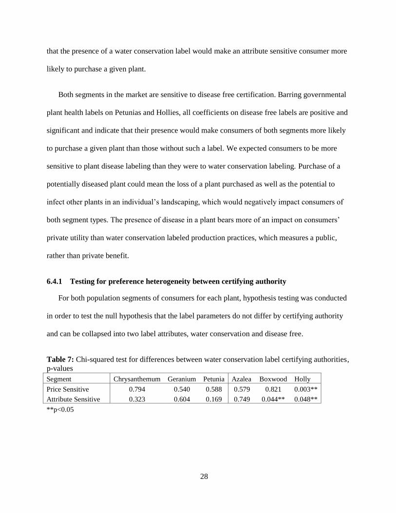
6.4.1 Testing for preference heterogeneity between certifying authority

For both population segments of consumers for each plant, hypothesis testing was conducted

in order to test the null hypothesis that the label parameters do not differ by certifying authority

and can be collapsed into two label attributes, water conservation and disease free.

Table 7: Chi-squared test for differences between water conservation label certifying authorities,

p-values


Price Sensitive 0.794 0.540 0.588 0.579 0.821 0.003**

Attribute Sensitive 0.323 0.604 0.169 0.749 0.044** 0.048**

**p<0.05

29

Table 8: Chi-squared test for differences between disease free label certifying authorities, p-

values


Price Sensitive 0.502 0.546 0.797 0.454 0.515 0.148

Attribute Sensitive 0.578 0.041** 0.510 0.550 0.520 0.471

**p<0.05

We fail to reject the null hypothesis in the case that there is no preference heterogeneity in

regards to certifying authority in all cases besides both segments of Holly consumers and the

attribute sensitive segment of Boxwood consumers. Additionally, we fail to reject the null

hypothesis that there is no preference heterogeneity between certifying authority for all cases

besides attribute sensitive Geranium consumers. Testing at the 10% level of significance, we

expected that approximately 3 of these tests would be rejected due to random chance and as

such, the results of this testing strongly suggest that consumers do not have heterogeneous

preferences for certifying authorities of either label type. These results were expected and are

consistent with Hartter et al. (2012).

7. Discussion and Conclusions

Our findings indicate that respondents show a positive and significant response to water

conservation and healthy plant labels. We found that for most of the six plants studied, neither

segment showed a preference for the certifying authority of either disease free or water

conservation labels. In light of these findings, it is suggested that additional research pertaining

to the potential for differing governmental, nongovernmental and industry groups to offer such

certification schemes be conducted. The matter of how such a labeling scheme could be

implemented by any certifying authority should be investigated further in order to successfully

market water conservation and disease free labeled plants to consumers of both price and

attribute sensitive market segments.

30

Our findings suggest that while one segment can be characterized by increased price

sensitivity, another segment is more attribute sensitive. The attribute sensitive segments were

generally more responsive to physical plant attributes, such as density and bloom levels, while

the price sensitive segments showed more concern for price than density and bloom

characteristics. Both segments were similarly sensitive to healthy plant labels, with slightly less

sensitivity to water conservation labels among price sensitive respondents than those who were

attribute sensitive.

Our results are suggestive of the possibility of selling a mix of both labeled and non-labeled

plants at the retail level. An assessment of segment characteristics indicates that there is a group

of attribute sensitive consumers more likely to purchase a labeled plant at a higher price, and a

price sensitive group of consumers more likely to buy a non-labeled plant at a lower price.

Given that retailers will not be able to distinguish between differing consumer segments, offering

a mix of both product types may be advantageous for sellers. By doing so, retailers have the

potential to draw in both consumer bases while also benefiting from any increased revenues

which may be gained through sales of additional products during store visits from this more

diverse group of customers. Lower sales prices that producers may be able to command by

selling non-labeled plants are expected to be offset by those higher value labeled sales to those

willing to pay a higher premium on disease free and water conservation labels.

While our estimates for the share of price versus attribute sensitive consumers in the market

for each plant studied can serve as a starting point for setting the level of labeled versus non-

labeled plants at retailers, it is suggested that further research be conducted on profitable product

mixes across plant types, retailers and geographic areas. Furthermore, it is also suggested that

future research investigate the price premiums gained for labels in a retail setting. Given that our

31

sampling techniques may have omitted individuals who would have entered the markets for

plants bearing a label, future research may also investigate how the makeup of the market for

each ornamental plant studied may change upon introduction of these labeling schemes.

32

References

Ajzen, I. 1991. “The Theory of Planned Behavior.” Organizational Behavior and Human

Decision Processes 50:179–211.

Albrecht, D., G. Bultena, E. Hoiberg, and P. Nowak. 1982. “Measuring Environmental Concern:

The New Environmental Paradigm Scale.” The Journal of Environmental Education

13(3):39–43.

Amburgey, J.W., and D.B. Thoman. 2012. “Dimensionality of the New Ecological Paradigm:

Issues of Factor Structure and Measurement.” Environment and Behavior 44(2):234–256.

Atkinson, I., G. Creighton, R. Fitzell, J. Gillett, G. McLennan, G. Robertson, C. Rolfe, G.

Seymour, I. Vimpany, D. Wilson, and B. Yiasoumi. 1994. Managing Water in Plant

Nurseries. NSW, Australia: Horticultural Research and Development Corportation, Nursery

Industry Association of Australia and NSW Agriculture.

Baksi, S., and P. Bose. 2007. “Credence goods, efficient labelling policies, and regulatory

enforcement.” Environmental and Resource Economics 37:411–430.

Behe, B. 2006. “Comparison of Gardening Activities and Purchases of Homeowners and

Renters.” J. Environ. Hort. 24(December):217–220.

Behe, B.K., B.L. Campbell, C.R. Hall, H. Khachatryan, J.H. Dennis, and C. Yue. 2013.

“Consumer Preferences for Local and Sustainable Plant Production Characteristics.”

HortScience 48(2):200–208.

Behe, B.K., and J.H. Dennis. 2009. “Age Influences Gardening Purchases , Participation , and

Customer Satisfaction and Regret.” Horticultural Economics and Management XVI:179–

184.

Best, H., and J. Mayerl. 2013. “Values, beliefs, attitudes: An empirical study on the structure of

environmental concern and recycling participation.” Social Science Quarterly 94(3):691–

714. Available at: 10.1111/ssqu.12010.

Birgelen, M. Van, J. Semeijn, and M. Keicher. 2009. “Proenvironmental Consumption Behavior

Investigating Purchase and Disposal.” Environment And Behavior 41(1):125–146.

Blend, J., and E.O. Van Ravenswaay. 1999. “Measuring Consumer Demand For Ecolabeled

Apples.” American Journal of Agricultural Economics 81(5):1072–1077.

Boxall, P.C., and W.L. Adamowicz. 2002. “Understanding heterogeneous preferences in random

utility models: A latent class approach.” Environmental and Resource Economics 23:421–

446.

33

Brécard, D., B. Hlaimi, S. Lucas, Y. Perraudeau, and F. Salladarré. 2009. “Determinants of

demand for green products: An application to eco-label demand for fish in Europe.”

Ecological Economics 69:115–125. Available at:

http://dx.doi.org/10.1016/j.ecolecon.2009.07.017.

Chen, T.B., and L.T. Chai. 2010. “Attitude towards the Environment and Green Products:

Comsumers‟ Perspective.” Management and Science Engineering 4(2):27–39.

Clark, C.F., M.J. Kotchen, and M.R. Moore. 2003. “Internal and external influences on pro-

environmental behavior: Participation in a green electricity program.” Journal of

Environmental Psychology 23:237–246.

Collart, A.J., M. a. Palma, and C.R. Hall. 2010. “Branding awareness and willingness-to-pay

associated with the Texas Superstar and Earth-Kind brands in Texas.” HortScience

45(8):1226–1231.

Crespi, J.M., and S. Marette. 2001. “Some Economic Implications of Public Labeling.” :83–94.

Cultice, A.K., D.J. Bosch, J.W. Pease, and K.J. Boyle. 2013. “Horticultural Producers ‟

Willingness to Adopt Water Recycling Technology in the Mid-Atlantic Region

Horticultural Producers ‟ Willingness to Adopt Water Recycling Technology in the Mid-

Atlantic Region Alyssa K . Cultice.”

Curtis, K.R., and M.W. Cowee. 2010. “Are homeowners willing to pay for „Origin-certified‟

plants in water-conserving residential landscaping?” Journal of Agricultural and Resource

Economics 35(1):118–132.

Dennis, J.H., and B.K. Behe. 2007. “Evaluating the role of ethnicity on gardening purchases and

satisfaction.” HortScience 42(2):262–266.

Dulleck, U., and R. Kerschbamer. 2006. “On Doctors, Mechanics, and Computer Specialists:

The Economics of Credence Goods.” Journal of Economic Literature 44(1):5–42.

Dunlap, R.E. 2008. “The New Environmental Paradigm Scale: From Marginality to Worldwide

Use.” The Journal of Environmental Education 40(January 2015):3–18.

Ebreo, A., J. Hershey, and J. Vining. 1999. “Reducing Solid Waste: Linking Recycling to

Environmentally Responsible Consumerism.” Environment And Behavior 31(1):107–135.

Edgell, M.C.R., and D.E. Nowell. 1989. “The new environmental paradigm scale: Wildlife and

environmental beliefs in British Columbia.” Society & Natural Resources 2(1):285–296.

Field, A., and J. Miles. 2010. “Exploratory Factor Analysis.” In Discovering Statistics using SAS.

Los Angeles, CA: SAGE Publications Inc., pp. 541–593.

34

Folger, P., B.A. Cody, and N.T. Carter. 2013. “Drought in the United States : Causes and Issues

for Congress.”

Galarraga Gallastegui, I. 2002. “The use of eco-labels: A review of the literature.” European

Environment 12:316–331.

Gardner, J.G., D.B. Eastwood, J.R. Brooker, J.B. Riley, W.E. Klingeman, and L. Systems. 2002.

“Consumers ‟ Willingness-To-Pay for Powdery Mildew Resistant Flowering Dogwoods.”

Gilg, A., and S. Barr. 2006. “Behavioural attitudes towards water saving? Evidence from a study

of environmental actions.” Ecological Economics 57:400–414.

Hartter, D.L., K.J. Boyle, J.W. Pease, K. Moeltner, and J.R. Harris. 2012. “Understanding

consumers ‟ ornamental plant preferences for disease-free and water conservation labels.”

Hedlund, T. 2011. “The Impact of Values, Environmental Concern, and Willingness to Accept

Economic Sacrifices to Protect the Environment on Tourists‟ Intentions to Buy Ecologically

Sustainable Tourism Alternatives.” Tourism and Hospitality Research 11(4):278–288.

Available at: http://thr.sagepub.com/content/11/4/278.abstract.

Hemmelskamp, J., and K.L. Brockmann. 1997. “Environmental labels - the German „Blue

Angel.‟” Futures 29(1):67–76.

Holmes, T.P., and W.L. Adamowicz. 2003. “Attrubute-Based Methods.” In P. A. Champ, K. J.

Boyle, and T. C. Brown, eds. A Primer on Nonmarket Valuation. pp. 171–213.

Hong, C.X., and G.W. Moorman. 2005. “Plant Pathogens in Irrigation Water: Challenges and

Opportunities.” Critical Reviews in Plant Sciences 24(3):189–208.

Hurtubia, R., M.H. Nguyen, A. Glerum, and M. Bierlaire. 2014. “Integrating psychometric

indicators in latent class choice models.” Transportation Research Part A: Policy and

Practice 64:135–146. Available at:

http://www.sciencedirect.com/science/article/pii/S0965856414000755 [Accessed April 20,

2015].

James, J.S., B.J. Rickard, and W.J. Rossman. 2009. “Product Differentiation and Market

Segmentation in Applesauce : Using a Choice Experiment to Assess the Value of Organic ,

Local , and Nutrition Attributes.” 3(December):357–370.

Khachatryan, H., B. Campbell, C. Hall, B. Behe, C. Yue, and J. Dennis. 2014. “The effects of

individual environmental concerns on willingness to pay for sustainable plant attributes.”

HortScience 49(June 2013):69–75.

Klingeman, W.E., D.B. Eastwood, J.R. Brooker, C.R. Hall, B.K. Behe, and P.R. Knight. 2004.

“Consumer Survey Identifies Plant Management Awareness and Added Value of Dogwood

Powdery Mildew Resistance.” HortTechnology 14(2):275–282.

35

Kollmuss, A., and J. Agyeman. 2002. “Mind the Gap: Why do people act environmentally and

what are the barriers to pro-environmental behavior?” Environmental Education Research

8(January 2015):239–260.

Kotchen, M.J., and S.D. Reiling. 2000. “Environmental attitudes, motivations, and contingent

valuation of nonuse values: A case study involving endangered species.” Ecological

Economics 32:93–107.

Lancaster, K.J. 1966. “A new approach to consumer theory.” The Journal of Political Economy

74(2):132.

Maryland Department of The Environment. 2012. “Maryland‟s Phase II Watershed

Implementation Plan for the Chesapeake Bay TMDL.”

McFadden, D. 1974. “Conditional logit analysis of qualitative choice behavior.” In P. Zarambka,

ed. Frontiers in Econometrics. Academic Press, pp. 105–142.

Michaud, C., D. Llerena, and I. Joly. 2012. “Willingness to pay for environmental attributes of

non-food agricultural products: A real choice experiment.” European Review of

Agricultural Economics:1–17.

Milon, J.W., and D. Scrogin. 2006. “Latent preferences and valuation of wetland ecosystem

restoration.” Ecological Economics 56:162–175. Available at:

http://www.sciencedirect.com/science/article/pii/S0921800905000571 [Accessed April 14,

2015].

Moorman, G. 2010a. “Phytophthora root rot, stem rot and cankers on ornamentals.” Plant

Disease Fact Sheets. Available at: http://extension.psu.edu/pests/plant-diseases/all-fact-

sheets/phytophthora-root-rot-on-woody-ornamentals.

Moorman, G. 2010b. “Pythium.” Plant Disease Fact Sheets. Available at:

http://extension.psu.edu/pests/plant-diseases/all-fact-sheets/pythium [Accessed January 1,

2015].

Morey, E., J. Thacher, and W. Breffle. 2006. “Using Angler Characteristics and Attitudinal Data

to Identify Environmental Preference Classes: A Latent-Class Model.” Environmental &

Resource Economics 34:91–115. Available at: http://link.springer.com/10.1007/s10640-

005-3794-7.

Morey, E., M. Thiene, M. De Salvo, and G. Signorello. 2008. “Using attitudinal data to identify

latent classes that vary in their preference for landscape preservation.” Ecological

Economics 68:536–546. Available at: http://dx.doi.org/10.1016/j.ecolecon.2008.05.015.

Noblet, C.L., M.F. Teisl, and J. Rubin. 2006. “Factors affecting consumer assessment of eco-

labeled vehicles.” Transportation Research Part D: Transport and Environment 11:422–

431.

36

Pacifico, D., and H. Yoo. 2012. “lclogit : A Stata module for estimating latent class conditional

logit models via the Expectation-Maximization algorithm.” … Australian School of

Business Research Paper. Available at:

http://papers.ssrn.com/sol3/papers.cfm?abstract_id=2174146.

Rees, G., A. Cultice, J. Pease, D. Bosch, and K. Boyle. 2014. “Irrigation Systems and Practices

in Mid-Atlantic Nurseries.”

Roberts, J.A., and D.R. Bacon. 1997. “Exploring the Subtle Relationships between

Environmental Concern and Ecologically Conscious Consumer Behavior.” Journal of

Business Research 40:79–89.

Rotherham, T. 1999. “Selling Sustainable Development: environmental labeing and certification

programs.” Available at: http://www.iisd.org/standards/pdf/miami_paper_final.pdf.

Schultz, P. 2001. “The structure of environmental concern: concern for self, other people, and

the biosphere.” Journal of Environmental Psychology 21(4):327–339. Available at:

http://linkinghub.elsevier.com/retrieve/pii/S0272494401902270 [Accessed October 9,

2014].

Smith, W.R. 1956. “Product differentiation and market segmentation as alternati.” Journal of

Marketing 21(1):3–8.

Sorice, M.G., W. Haider, J.R. Conner, and R.B. Ditton. 2011. “Incentive Structure of and Private

Landowner Participation in an Endangered Species Conservation Program.” Conservation

Biology 25(3):587–596.

Swait, J. 1994. “A structural equation model of latent segmentation and product choice for cross-

sectional revealed preference choice data.” Journal of Retailing and Consumer Services

1(2):77–89.

Tarrant, M.A., and H.K. Cordell. 1997. “The Effect of Respondent Characteristics on General

Environmental Attitude-Behavior Correspondence.” Environment And Behavior 29(5):618–

637.

Teisl, M., B. Roe, and R. Hicks. 2002. “Can eco-labels tune a market? Evidence from dolphin-

safe labeling.” Journal of Environmental Economics and Management 43:339–359.

Available at: http://www.sciencedirect.com/science/article/pii/S0095069600911860.

Teisl, M.F., and B. Roe. 1998. “The economics of labeling: an overview of issues for health and

environmental disclosure.” Agricultural and Resource Economics Review 27:140 – 150.

Thapa, B. 2001. “Environmental Concern: A comparative analysis between students in

Recreation and Park Management and other departments.” Environmental Education

Research 7(1):39–53.

37

The National Drought Mitigation Center. 2015. “Drought Condition (Percent Area): United

States.” Available at: http://droughtmonitor.unl.edu/Home/TabularStatistics.aspx [Accessed

January 1, 2015].

Thøgersen, J. 2002. “Promoting green consumer behavior with eco-labels.” In T. Dietz and P.

Stern, eds. New Tools for Environmental Protection: Education, Informantion, and

Voluntary Measures. Washington DC: national Academy Press, pp. 83–104.

United States Department of Agriculture. 2010. “Census of Horticultural Specialties (2009).”

Available at: papers2://publication/uuid/FB6B726A-B11C-47FB-9A8A-AA16AB3CCCF1.

United States Department of Agriculture National Agricultural Statistics Service. 2014. “2012

Census of Agriculture.”

Wicker, P., and S. Becken. 2013. “Conscientious vs. ambivalent consumers: Do concerns about

energy availability and climate change influence consumer behaviour?” Ecological

Economics 88:41–48. Available at: http://dx.doi.org/10.1016/j.ecolecon.2013.01.005.

Williams-Woodward, J. 2013. “Georgia Plant Disease Loss Estimates.”

Willis, R.M., R.A. Stewart, K. Panuwatwanich, P.R. Williams, and A.L. Hollingsworth. 2011.

“Quantifying the influence of environmental and water conservation attitudes on household

end use water consumption.” Journal of environmental management 92(8):1996–2009.

Available at: http://www.sciencedirect.com/science/article/pii/S0301479711000892

[Accessed August 8, 2014].

Wolters, E.A. 2014. “Attitude–behavior consistency in household water consumption.” The

Social Science Journal 51(3):455–463. Available at:

http://www.sciencedirect.com/science/article/pii/S036233191300147X [Accessed January

21, 2015].

Yue, C., C.R. Hall, B.K. Behe, B.L. Campbell, J.H. Dennis, and R.G. Lopez. 2010. “Are

Consumers Willing to Pay More for Biodegradable Containers Than for Plastic Ones ?

Evidence from Hypothetical Conjoint Analysis and Nonhypothetical Experimental

Auctions.” J. Agric. Appl. Econ. 42(November):757–772.

Yue, C., T.M. Hurley, and N. Anderson. 2011. “Do native and invasive labels affect consumer

willingness to pay for plants? Evidence from experimental auctions.” Agricultural

Economics 42:195–205.

38

Appendix A: Depiction of Labeling Information

Figure A-1: Water conservation certification labels

Label Description

None 'None' describes a plant that is grown using typical

watering practices.

A choice labeled 'Water Smart' by the U.S. Department

of Agriculture (USDA) means the ornamental plants

were grown to meet U.S. Department of Agriculture

requirements concerning water conservation and

produced with water recycling technology. The USDA

is a government agency charged with developing

policy concerning farming, food and agriculture. The

certification implies producers are regularly audited

and monitored by the USDA to ensure requirements

are met.

A choice labeled 'Water Smart' by the American

Nursery Association (ANA) means the ornamental

plants were grown to meet American Nursery

Association requirements concerning water

conservation and produced with water recycling

technology. The American Nursery Association is an

industry association representing the producers of

ornamental plants. The certification implies producers

are regularly audited and monitored by the industry

association to ensure requirements are met.

A choice labeled 'Water Smart' by Water for

Tomorrow means the ornamental plants were grown to

meet Water for Tomorrow requirements concerning

water conservation and produced with water recycling

technology. Water for Tomorrow is an environmental

non-governmental organization (NGO) which

advocates for the protection of public water resources.

Examples of other NGO's in the U.S. are the Sierra

Club and The Forest Stewardship Council. The

certification implies producers are regularly audited

and monitored by Water for Tomorrow to ensure

requirements are met.

Source: Hartter et al. 2012

39

Figure A-2: Disease-free certification labels

Label Description

None 'None' describes a plant that has no plant health

certification.

A choice labeled 'Healthy Plants - Certified Disease

Free' by the U.S. Department of Agriculture (USDA)

means the plant was grown under conditions that meet

U.S. Department of Agriculture (USDA) requirements

to ensure the plant is free of disease and healthy. The

USDA is a government agency charged with developing

policy concerning farming, food and agriculture. The

certification implies plants and producers are regularly

audited and monitored by the USDA to ensure

requirements are met.

A choice labeled „Healthy Plants - Certified Disease

Free‟ by the American Nursery Association (ANA)

means the plant was grown under conditions that meet

American Nursery Association requirements to ensure

the plant is free of disease and healthy. The American

Nursery Association is an industry association

representing the producers of ornamental plants. The

certification implies the plants producers are regularly

audited and monitored by the industry association to

ensure requirements are met.

A choice labeled „Healthy Plants - Certified Disease

Free‟ by Plant Society of America means the plant was

grown under conditions that meet Plant Society of

America requirements to ensure the plant is free of

disease and healthy. Plant Society of American is a

gardening organization promoting gardening and

healthy plants. The certification implies the plants

producers are regularly audited and monitored by Plant

Society of America to ensure requirements are met.


40

Appendix B: Choice Experiment Design

Table B-1: Choice experiment attributes and levels

Attribute Level Value Variable Name Description

Bloom 2 Low Bloom Omitted Less than 30% of the buds are in bloom

1 Partial Bloom Partialbloom 30 to 70% of the buds are in bloom

0 Full Bloom Fullbloom 80 to 100% of the buds are in bloom

Fullness 2 Light Omitted The plant has a light density of foliage

1 Medium Medium The plant has a medium density of

foliage

0 Full Full The plant has a full density of foliage

Water

Conservation 3 ENGO Certification ENGOWC

Certified for water conservation by

Water for Tomorrow, a non-

governmental organization

2 ANA Certification ANAWC

Certified for water conservation by

American Nursery Association, an

industry organization

1 USDA Certification USDAWC

Certified for water conservation by the

United States Department of

Agriculture, a government agency

0 None Omitted No water conservation certification

Plant Health 3 GO Certification GOPH

Certified disease-free by Plant Society

of America, a gardening non-

governmental organization

2 ANA Certification ANAPH

Certified disease-free by American

Nursery Organization, and industry

association

1 USDA Certification USDAPH

Certified disease-free by the United

States Department of Agriculture, a

government agency

0 None Omitted No disease-free certification

Price ($) Chrysanthemum Geranium Petunia

3 6.53 6.04 4.54

2 5.53 4.84 3.84

1 4.54 3.64 3.15

0 3.54 2.44 2.45

Azalea Boxwood Holly

3 7.04 12.74 15.78

2 5.7 10.81 12.5

1 4.37 8.87 2.22

0 3.03 6.94 5.94


41

Table B-2: Bedding plant choice experiment design Choice 1 A B Choice 9 A B

Bloom 2 0 Bloom 0 1

Fullness 0 1 Fullness 2 1

Water Conservation 3 2 Water Conservation 2 0

Plant Health 2 0 Plant Health 3 2

Price 2 1 Price 0 2

Choice 2 A B Choice 10 A B

Bloom 0 2 Bloom 0 2




Price 3 0 Price 2 0


Bloom 0 1 Bloom 1 2




Price 0 3 Price 0 3


Bloom 1 0 Bloom 1 0




Price 1 1 Price 2 1


Bloom 2 2 Bloom 1 2




Price 2 3 Price 3 0


Bloom 2 1 Bloom 0 1




Price 0 3 Price 3 0


Bloom 2 0 Bloom 2 0




Price 1 2 Price 1 2


Bloom 1 0 Bloom 0 1




Price 1 2 Price 3 1


42

Table B-3: Azalea choice experiment design





Price 1 0 Price 2 0





Price 2 3 Price 1 0





Price 0 2 Price 1 3





Price 2 1 Price 3 3





Price 3 0 Price 0 1





Price 1 1 Price 3 2





Price 0 2 Price 0 2





Price 3 3 Price 2 1


43

Table B-4: Boxwood and Holly choice experiment design





Price 2 0 Price 3 2





Price 2 0 Price 3 0





Price 2 1 Price 1 3





Price 0 1 Price 0 2





Price 0 1 Price 0 2





Price 2 3 Price 1 0





Price 3 2 Price 1 3





Price 3 1 Price 1 3


44

Appendix C: Factor Analysis Results

Table C-1: R-matrix of correlation coefficients for New Environmental Paradigm scale items

New Environmental Paradigm Scale Item Correlations

nep1 Rnep2 nep3 Rnep4 nep5 Rnep6 nep7 Rnep8 nep9 Rnep10 nep11 Rnep12 nep13 Rnep14 nep15

nep1 1.00 Rnep2 0.13 1.00

nep3 0.32 0.28 1.00 Rnep4 0.26 0.31 0.21 1.00

nep5 0.45 0.28 0.54 0.25 1.00 Rnep6 0.31 0.24 0.17 0.35 0.22 1.00

nep7 0.30 0.28 0.34 0.10 0.43 0.06 1.00 Rnep8 0.31 0.39 0.34 0.42 0.41 0.34 0.22 1.00

nep9 0.10 0.16 0.28 0.11 0.25 -0.01 0.25 0.11 1.00 Rnep10 0.40 0.41 0.35 0.40 0.48 0.36 0.32 0.60 0.16 1.00

nep11 0.51 0.18 0.34 0.24 0.43 0.30 0.28 0.34 0.21 0.38 1.00 Rnep12 0.24 0.37 0.25 0.28 0.30 0.25 0.36 0.40 0.15 0.45 0.24 1.00

nep13 0.33 0.25 0.46 0.21 0.50 0.17 0.37 0.36 0.21 0.41 0.36 0.26 1.00 Rnep14 0.11 0.24 0.14 0.37 0.12 0.25 0.07 0.30 0.18 0.24 0.12 0.29 0.03 1.00

nep15 0.54 0.29 0.47 0.29 0.63 0.28 0.38 0.39 0.21 0.58 0.52 0.29 0.55 0.11 1.00

Table C-2: Factor eigenvalues greater than one for varimax rotation results of New

Environmental Paradigm items

Factor Variance Difference Proportion Cumulative

Factor1 3.78346 1.06842 0.2522 0.2522

Factor2 2.71504 1.03152 0.181 0.4332

Factor3 1.68352 . 0.1122 0.5455

45

Figure C-1: Screeplot of eigenvalues for factors one through fifteen of New Environmental

Paradigm items

02

46

Eig

enva

lues

0 5 10 15Number

Scree plot of eigenvalues after factor

46

Table C-3: Varimax rotated factor loadings of New Environmental paradigm items with three

retained factors

Rotated Factor Loadings

Variable Factor1 Factor2 Factor3

nep1 0.7569 0.1331 -0.1192

Rnep2 0.1200 0.5757 0.3704

nep3 0.5361 0.1382 0.4348

Rnep4 0.2230 0.6800 -0.0763

nep5 0.7092 0.1521 0.3354

Rnep6 0.3654 0.5438 -0.3457

nep7 0.3934 0.0716 0.5976

Rnep8 0.4039 0.6250 0.0849

nep9 0.0895 0.0936 0.6660

Rnep10 0.5453 0.5434 0.1381

nep11 0.7107 0.1456 0.0010

Rnep12 0.1968 0.5596 0.3349

nep13 0.6346 0.0721 0.3484

Rnep14 -0.0972 0.7041 0.1170

nep15 0.8022 0.1743 0.1762

Table C-4: Kaiser-Meyer-Olkin (KMO) measure of sampling adequacy for New Environmental

Paradigm scale items

Variable KMO

nep1 0.8940

Rnep2 0.9143

nep3 0.9214

Rnep4 0.9017

nep5 0.9194

Rnep6 0.9003

nep7 0.8839

Rnep8 0.8985

nep9 0.8275

Rnep10 0.9003

nep11 0.9128

Rnep12 0.9030

nep13 0.9249

Rnep14 0.8016

nep15 0.8923

Overall 0.9002

47

Appendix D: Latent Class Segmentation Results


in annual bedding plants

Chrysanthemum Geranium Petunia

Segments CAIC BIC Segments CAIC BIC Segments CAIC BIC

2 2652.7 2626.7 2 2823.9 2797.9 2 2786.7 2760.7

3 2691.9 2651.9 3 2888.3 2848.3 3 2798.3 2758.3

4 2774.9 2720.9 4 2969.8 2915.8 4 2899.1 2845.1

5 2856.5 2788.5 5 3051.5 2983.5 5 2995.3 2927.3

6 2964.2 2882.2 6 3130.1 3048.1 6 3081.5 2999.5

7 3044.6 2948.6 7 3250.0 3154.0 7 3167.2 3071.2

8 3155.3 3045.3 8 3341.8 3231.8 8 3230.8 3120.8

9 3246.5 3122.5 9 3417.0 3293.0 9 3357.3 3233.3

10 3380.6 3242.6 10 3516.9 3378.9 10 3474.8 3336.8


in broadleaf evergreen plants

Azalea Boxwood Holly

Segments CAIC BIC Segments CAIC BIC Segments CAIC BIC

2 2624.1 2602.1 2 1904.8 1882.8 2 1860.3 1838.3

3 2655.8 2621.8 3 1920.9 1886.9 3 1877.0 1843.0

4 2699.9 2653.9 4 1972.2 1926.2 4 1945.9 1899.9

5 2783.4 2725.4 5 2044.6 1986.6 5 2020.1 1962.1

6 2898.6 2828.6 6 2113.8 2043.8 6 2097.6 2027.6

7 2947.8 2865.8 7 2211.9 2129.9 7 2183.6 2101.6

8 3034.4 2940.4 8 2288.9 2194.9 8 2252.9 2158.9

9 3119.2 3013.2 9 2366.9 2260.9 9 2339.4 2233.4

10 3228.4 3110.4 10 2448.3 2330.3 10 2425.6 2307.6

48

Appendix E: Example Stata Codes for Latent Class Model

*Generate variables

gen ASC = a | b

*Reverse-code even-numbered NEP variables

gen Rnep2 = 6 - nep2







*Install plug-in program

ssc install gllamm

*Petunia Analysis

use "D:\Thesis\Data, Do Files, Results\Data\Petunia.dta"

drop if nep1 == .

*Determine the # of classes (Both hole and lclogit code journal

forvalues c= 2/10 {

quietly lclogit choice price ASC partialbloom fb medium full usdawc anawc engowc usdaph

anaph goph, group(gid) id(pid) nclass(`c') membership(nepsum) seed(5)

matrix b=e(b)

matrix ic = nullmat(ic) \ è(nclasses)', è(ll)', `=colsof(b)', è(aic)', è(caic)', è(bic)'

}

matrix colnames ic = "Classes" "LLF" "Nparam" "AIC" "CAIC" "BIC"

matlist ic, name(columns)

*estimate the latent class model with 2 classes

lclogit choice price ASC partialbloom fb medium full usdawc anawc engowc usdaph anaph

goph, group(gid) id(pid) nclass(2) membership(nepsum) seed(5)

*get the prior and posterior class membership probabilities

lclogitpr prior, up

lclogitpr post, cp

*get the conditional and unconditional choice probabilities

lclogitpr cpr, pr

*attributes coefficient means and covariances

matrix list e(PB)

49

*get class-specifc inferences

lclogitml, iterate(10)

*Assign respondents to a class

gen class=1

replace class=2 if post2>post1

*Conduct label collapsing tests

test _b[choice1: usdawc] = _b[choice1: anawc] = _b[choice1: engowc]

test _b[choice1: usdaph] = _b[choice1: anaph] = _b[choice1: goph]

test _b[choice2: usdawc] = _b[choice2: anawc] = _b[choice2: engowc]

test _b[choice2: usdaph] = _b[choice2: anaph] = _b[choice2: goph]

<repeat similar script for remaining plants>

50

Appendix F: New Environmental Paradigm Responses

Table F-1: Average respondent scores on New Environmental Paradigm items, by segment and

plant


Price

Sensitive

Segment

NEPsum 38.404 38.604 38.765 39.075 40.112 38.313

Nep1 2.693 2.769 2.760 2.779 2.840 2.807

Rnep2* 2.778 2.709 2.734 2.789 2.963 2.659

Nep3 2.224 2.258 2.292 2.305 2.364 2.295

Rnep4* 3.089 3.011 3.065 3.146 3.171 3.131

Nep5 2.111 2.203 2.170 2.232 2.246 2.210

Rnep6* 3.667 3.632 3.655 3.669 3.733 3.670

Nep7 1.991 2.176 1.991 2.026 2.160 2.028

Rnep8* 2.630 2.451 2.609 2.619 2.711 2.534

Nep9 1.741 1.709 1.753 1.727 1.781 1.750

Rnep10* 2.704 2.654 2.737 2.787 2.840 2.670

Nep11 2.398 2.445 2.471 2.458 2.594 2.386

Rnep12* 2.700 2.945 2.765 2.763 2.840 2.608

Nep13 2.189 2.302 2.226 2.269 2.337 2.222

Rnep14* 2.865 2.670 2.765 2.826 2.754 2.705

Nep15 2.622 2.670 2.639 2.680 2.781 2.636

Attribute

Sensitive

Segment

NEPsum 38.968 38.877 39.532 37.769 38.288 38.385

Nep1 2.899 2.775 2.858 2.654 2.767 2.678

Rnep2* 2.661 2.739 2.865 2.635 2.641 2.752

Nep3 2.228 2.251 2.142 2.077 2.233 2.266

Rnep4* 3.048 3.140 3.277 2.853 3.087 3.059

Nep5 2.265 2.173 2.277 2.115 2.139 2.157

Rnep6* 3.741 3.676 3.801 3.667 3.680 3.622

Nep7 2.106 1.976 2.170 2.038 1.932 2.010

Rnep8* 2.492 2.650 2.546 2.519 2.560 2.577

Nep9 1.683 1.754 1.745 1.718 1.673 1.671

Rnep10* 2.720 2.771 2.716 2.551 2.748 2.654

Nep11 2.460 2.467 2.461 2.397 2.427 2.406

Rnep12* 2.979 2.717 2.901 2.897 2.803 2.811

Nep13 2.296 2.229 2.270 2.218 2.162 2.196

Rnep14* 2.730 2.899 2.709 2.859 2.858 2.892

Nep15 2.661 2.659 2.794 2.571 2.579 2.633

*Denotes items have been reverse coded to keep directionality of scale consistent. Higher scores indicate

levels of environmentalism. A full description of each item can be found in Table 2.

51

Appendix G: Respondent Summary Statistics

Table G-1: Summary statistics of socio-demographic characteristics (n = 745)

Demographic variables Percentage Percentage

Gender Male 28.9%

Income <$20k 2.8%

Female 69.9%

$20k to $40k 10.1%

$40k to $60k 17.2%

Race Asian 2.8%

$60k to $80k 16.1%

Black 0.4%

$80k to $100k 16.4%

White 90.9%

$100k to $120k 12.2%

Other 5.9%

$120k to $140k 6.8%

$140k to $160k 6.6%

Education Some high school or

less 0.4%

$160k to $180k 3.4%

High school graduate 8.6%

$180k to $200k 3.1%

Some technical school 3.6%

$200k to $300k 3.4%

Some college 24.4%

>$300k 2.0%

College graduate 30.2%

Master's degree 24.7%

Age Mean 55.19

Doctorate degree 4.8%

Standard Deviation 13.56

Professional degree 3.2%

Household Size Mean 2.41 Housing

Type Detached house 82.8%

Standard Deviation 1.25

Attached house 13.0%

Apartment 3.6%

Years in Residence Mean 14.82

Other 0.5% Standard Deviation 11.91

Date post:	04-Nov-2018
Category:	Documents
Upload:	phungtruc
View:	215 times
Download:	0 times

The effect of environmental preferences on the market for eco … · Segmentation of the market for...

Documents