The Effect of Ionizing Gamma and Beta Radiation on Phaseolus vulgaris Growth and Aerogel Optical Properties Abstract: Radiation affects human life in disparately subtle and dramatic ways. For instance, nuclear reactions in the Sun produce light and heat that are essential for human existence, while recent research implies that the flux of cosmic ray particles may also have an impact on humans’ daily lives. According to the EPA the average American receives 3100 micro Sieverts (μ Sv) of radiation per year, well under a total dose of 500,000 (μ Sv) and higher doses that cause symptoms ranging from nausea to death. However, scientists hypothesize that exposure to low doses of ionizing radiation (< 10,000 μ Sv) may produce beneficial effects in organisms. Thus the effect of low doses of beta, and gamma radiation (8 doses ranging from total dosages of 95 (μSv) ±10% gamma radiation to 1820 (μSv) ±10% beta radiation.) on Phaseolus vulgaris was tested. Results from this experiment showed a hormetic curve when analyzing the height of the plant, but because of a large amount of uncertainty made these results inconclusive. The same radiation was also tested on the performance of aerogel, a material used in particle detectors. Aerogel will be used in experiments at the 12 GeV Jefferson Laboratory and has been previously observed to change its optical characteristics after being used in experiments. Results from this experiment showed a significant decrease in percent transmittance when exposed to beta radiation, but not gamma radiation. To determine the level of cosmic ray flux and possible contribution to our experiments a detector was created using scintillator material and 2-inch phototubes. Results from our experiments will be presented. Results from this experiment show that more calculations and tests must be completed before verifying random coincidences.
Transcript
The Effect of Ionizing Gamma and Beta Radiation on Phaseolus vulgaris Growth and
Aerogel Optical Properties
Abstract:
Radiation affects human life in disparately subtle and dramatic ways. For instance,
nuclear reactions in the Sun produce light and heat that are essential for human existence, while
recent research implies that the flux of cosmic ray particles may also have an impact on humans’
daily lives. According to the EPA the average American receives 3100 micro Sieverts (μ Sv) of
radiation per year, well under a total dose of 500,000 (μ Sv) and higher doses that cause
symptoms ranging from nausea to death. However, scientists hypothesize that exposure to low
doses of ionizing radiation (< 10,000 μ Sv) may produce beneficial effects in organisms. Thus
the effect of low doses of beta, and gamma radiation (8 doses ranging from total dosages of 95
(μSv) ±10% gamma radiation to 1820 (μSv) ±10% beta radiation.) on Phaseolus vulgaris was
tested. Results from this experiment showed a hormetic curve when analyzing the height of the
plant, but because of a large amount of uncertainty made these results inconclusive. The same
radiation was also tested on the performance of aerogel, a material used in particle detectors.
Aerogel will be used in experiments at the 12 GeV Jefferson Laboratory and has been previously
observed to change its optical characteristics after being used in experiments. Results from this
experiment showed a significant decrease in percent transmittance when exposed to beta
radiation, but not gamma radiation. To determine the level of cosmic ray flux and possible
contribution to our experiments a detector was created using scintillator material and 2-inch
phototubes. Results from our experiments will be presented. Results from this experiment show
that more calculations and tests must be completed before verifying random coincidences.
Introduction:
This project was conducted to investigate the effect of low dosages of gamma and beta
radiation on life, in this specific case, Phaseolus vulgaris, also known as bush beans. Radiation is
the energy from waves or particles travelling at high speeds. This project tested ionizing
radiation, which is characterized by the ability to strip atoms of electrons. Ionizing radiation
requires more energy than non-ionizing and therefore only waves and particles in the ultraviolet
to gamma ray portion of the electromagnetic spectrum are considered ionizing. When an atom is
ionized two ions are formed and occasionally a chemical bond is broken. The body attempts to
rectify these problems, but sometimes the damage is beyond repair and other times mistakes are
made in the natural repairing process, which can in turn lead to cancerous cells. Therefore,
ionizing particles are particularly more dangerous than non-ionizing because their ability to alter
atomic structure offers the chance of damaging DNA, which, in turn, increases the chance of
cancer [1]. Radiation originates from a myriad of different sources. Most however, comes in the
form of alpha, beta, and gamma radiation from radionuclides (decaying radioactive elements or
isotopes). These radionuclides are naturally unstable – the forces holding the protons and
neutrons in the nucleus are unequal – and due to this fact, they attempt to reach stability by either
banishing neutrons and protons from the nucleus, altering a neutron to a proton or vice versa by
removing a beta particle from the nucleus, or by releasing excess energy within the nucleus in
the form of a photon/gamma ray [1]. The last two forms of compensation are beta and gamma
radiation respectively. These two types of radiation were tested on plant growth because alpha
radiation (ejection of neutrons and protons) is very weak and has low energy compared to the
others, making it trivial for such an experiment.
Humans and other life forms are exposed to radiation almost constantly, receiving an
average of 3100 μSv of ionizing radiation from the environment alone. The sources of this
natural background radiation comes from cosmic ray radiation, terrestrial radiation, internal
radiation in the organisms themselves as well as radon and Thoron gas emitted from the Earth’s
crust into the atmosphere. In addition to these background sources of radiation, even more
radiation is received through medical procedures, consumer products and nuclear medicine,
raising the average annual dose to approximately 6200 μSv [2].
Cosmic rays, one type of radiation humans are exposed to, originates from unknown
sources in space, emitting high energy leptons such as electrons and muons that decay in seconds
upon reaching Earth. Muons in particular are very easy to detect because of their relatively high
mass and high energy, making them ideal particles for triggering detector equipment. Berkeley
cosmic ray detectors are one such device that utilizes two or more scintillator paddles attached to
photomultiplier tubes (PMT), which in turn lead to electronic modules. The scintillators
effectively transform the energy of the muon into photons, which are then picked up by an array
of dynodes in the PMT which transfer that photon into a cascade of electrons, or in essence,
electric current. Since muons generally come from an angle relatively close to 90° (π), the
detectors are set some distance away directly lined up vertically. This ensures that most, but not
all, of the particles being detected by a Berkeley particle detector are indeed muons, and not
some other particle. Trigger efficiency and delay tests utilizing three or more paddles can be
conducted to quantify the number of particles being detected that are not muons. While all life is
exposed to cosmic rays, recent research hints at the fact that there are slight health effects gained
from too much exposure from cosmic rays, which differ based on altitude and other factors [3]
[4].
Since all life on Earth is, and always has been exposed to low dosages of radiation, low
levels of radiation on Earth are not completely lethal to organisms. This occurs because cells that
make up any and all organisms have adapted to almost constant radiation and counter its
negative influences, occasionally even reaping benefits from low dosages of radiation, a
phenomenon called hormesis. While the definitive reason and motives by which hormesis occurs
are unclear, many scientists hypothesize that an overcompensating response to the radiation by
cells actually improves factors such as growth or life span. However, in order to fit any sort of
data to a hormetic model, the intervals of dosages must be of the same scale as the expected dose
to produce a hormetic response [5]. Therefore, this project utilized a myriad of low dosages with
a couple higher dosages to try to fit a hormetic curve to the variables of leaf diameter, height of
plants, and number of leaves.
Extensive research has been conducted already on the effect of irradiation on plants, but
very few have been conducted on hormetic responses. Research shows that with high dosages of
gamma radiation, most plants will completely die, resulting in a high mortality rate [6]. In
intermediate dosages, abnormalities such as stimulated excessive growth, and misconstrued
leaves occur [6]. However, very few experiments are conducted at low dosages, which means
very few witness any sort of hormetic or beneficial effect on the plants. In fact, modern
toxicology tests only 3 or 4 very high dosages of any chemical carcinogen before extrapolating
down linearly to meet the moderately low dosages of radiation, etc. that humans are exposed to
[5]. Since the dose-response curve is most likely not linear and instead U or hill-shaped, this
means that the extrapolated data is incorrect or at least some degree off from the actual response.
Some experiments conducted by the Department of Nuclear Engineering at Osaka
University in Japan found absorbed dosages in the 1 cGy to 10 Gy say beneficial effects on both
the stem and root height of Raphanus sativus (radishes). This experiment utilized D-T neutron
radiation (reaction of deuterium and tritium to produce a neutron and 4He) to achieve this result,
and gamma ray radiation Co-60 used in the same experiment saw no positive effects [7].
Plants, as with other living organisms, respond to their environment in a myriad of ways,
and it is difficult to discern and limit all the variables affecting them. For instance, plants go
through a process called etiolation when growing in the absence of light, characterized by a pale,
long, and thin stem, and a smaller leaves [8]. Therefore, when experimenting with plants, it is
very important to attempt to limit the number of random variables, especially with variables
essential to the plants, such as light, water, and temperature.
In addition to testing the effect of radiation on bean plants, this project also tested the
effect of beta and gamma radiation on Aerogel, a product made from silica gel that has rather
unique innate properties, making it ideal for the detection of particles in Cherenkov detectors that
detect pions and kaons. Jefferson Laboratory in Newport News, Virginia uses Aerogel in
Cherenkov detectors in Hall C, some of which have been found to become discolored upon
staying in the detector for extended periods of time. Scientists at Jefferson Laboratory have
hypothesized that radiation from the high-energy particles causes the discoloration.
Materials & Methods:
Since this project encompassed three smaller, albeit related experiments, the three
experimental material and methods will be separated by bolded subtitles with the project title.
The Effect of Ionizing Radiation on Phaseolus vulgaris Growth and Development
For the effect of radiation on the growth and development of Phaseolus vulgaris, there
were two separate experiments were conducted: one tested different levels of radiation of beta
and gamma radiation on bean plants that began germination all on the same day, while the other
tested the same level of gamma radiation on plants in different stages of their development.
For the experiment of different dosages of gamma and beta radiation, Stringless Blue
Lake, FM1K (Pole) garden beans from Ferry Moss Co. were used. To germinate the beans, they
were placed individually into dampened paper towels and then placed into a paper bag taped to a
window on July 9th
, 2013. These beans germinated quickly, and were transplanted into five
boxes on Tuesday, July 16th
. The boxes dimensions were 320 mm x 270 mm by 200 mm, and
they were filled with 4.25 liters of Miracle Gro® Potting Soil, which amounted to a spoil depth
of approximately 5 cm. Each box had a plastic bag lining its bottom in order for the box not to
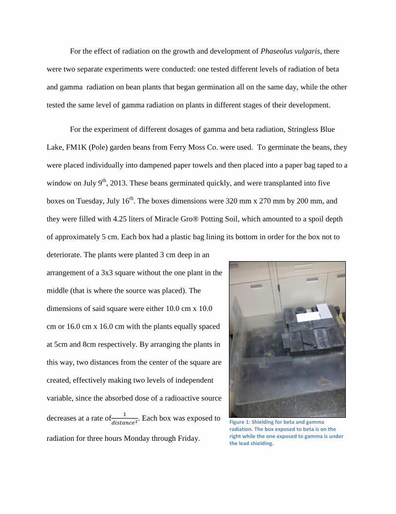
deteriorate. The plants were planted 3 cm deep in an
arrangement of a 3x3 square without the one plant in the
middle (that is where the source was placed). The
dimensions of said square were either 10.0 cm x 10.0
cm or 16.0 cm x 16.0 cm with the plants equally spaced
at 5cm and 8cm respectively. By arranging the plants in
this way, two distances from the center of the square are
created, effectively making two levels of independent
variable, since the absorbed dose of a radioactive source
decreases at a rate of
. Each box was exposed to
radiation for three hours Monday through Friday.
Figure 1: Shielding for beta and gamma radiation. The box exposed to beta is on the right while the one exposed to gamma is under the lead shielding.
Plastic shielding was utilized to protect from Beta radiation while lead shielding was used to
counter gamma radiation. The control box was put under a desk so as to be in the shade, and
receive approximately the same amount of light as the irradiated boxes. See Figure 1 for an
image of the shielding used for the experiment. See Table 1 below for a complete list of the
equivalent dosages each level of independent variable was exposed to.
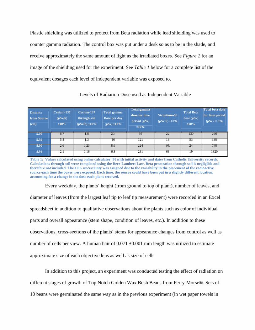
Levels of Radiation Dose used as Independent Variable
Distance
from Source
(cm)
Cesium-137
(μSv/h)
±10%
Cesium-137
through soil
(μSv/h) ±10%
Total gamma
Dose per day
(μSv) ±10%
Total gamma
dose for time
period (μSv)
±10%
Strontium-90
(μSv/h) ±10%
Total Beta
dose (μSv)
±10%
Total beta dose
for time period
(μSv) ±10%
5.00 6.7 1.8 20. 95 22 130 266
5.59 5.4 1.3 16 121 18 53 338
8.00 2.6 0.23 8.6 224 80. 24 748
8.94 2.1 0.16 6.8 281 63 19 1820
Table 1: Values calculated using online calculator [9] with initial activity and dates from Catholic University records.
Calculations through soil were completed using the Beer-Lambert Law. Beta penetration through soil is negligible and
therefore not included. The 10% uncertainty was assigned due to the variability in the placement of the radioactive
source each time the boxes were exposed. Each time, the source could have been put in a slightly different location,
accounting for a change in the dose each plant received.
Every weekday, the plants’ height (from ground to top of plant), number of leaves, and
diameter of leaves (from the largest leaf tip to leaf tip measurement) were recorded in an Excel
spreadsheet in addition to qualitative observations about the plants such as color of individual
parts and overall appearance (stem shape, condition of leaves, etc.). In addition to these
observations, cross-sections of the plants’ stems for appearance changes from control as well as
number of cells per view. A human hair of 0.071 ±0.001 mm length was utilized to estimate
approximate size of each objective lens as well as size of cells.
In addition to this project, an experiment was conducted testing the effect of radiation on
different stages of growth of Top Notch Golden Wax Bush Beans from Ferry-Morse®. Sets of
10 beans were germinated the same way as in the previous experiment (in wet paper towels in
plastic bags) one week apart from each other with five weeks total. The initial batch began
germination July 9th
, 2013, and the final batch began germination August 6th
, 2013. On that same
day, August 6th
, all five batches of plants were planted in pairs into pots with a diameter of 8.5 ±
0.5 cm in a soil depth of approximately 8 cm. One pot was set as a control while the other was
set as an experimental trial, making four plants for each separate age group. The plants that
began germination four weeks prior to the initiation of the experiment only had one plant in the
control group because poor germination results yielded only three plants usable in
experimentation. Exposure to Cs-137 gamma radiation began on Wednesday, August 7th
. The
dose rate of the radiation was 168 μSv ± 10%. These plants were analyzed daily much the same
way as the other experiments with the height, leaf diameter, number of leaves, and additionally
stem diameter recorded in excel for a period of one week. No qualitative observations were made
on this experiment due to the shorter time period of observation. These plants did not have their
cells analyzed. This experiment was conducted more to determine whether radiation had a more
significant effect on the plants’ on a specific stage of their growth.
Investigating Trigger Efficiency and Cosmic Ray Flux in a Berkeley Cosmic Ray Detector
Though this experiment tested the effect of radiation from radioactive isotopes on plant
growth, there are numerous other types of radiation discussed earlier that come in contact with
the plants as well. One of these types of radiation is cosmic ray radiation. In order to formulate a
numerical value for the radiation affecting the plants that originated from cosmic rays, a
Berkeley cosmic ray detector was utilized. The cosmic ray detector previously constructed at
Catholic University contained two Lucite scintillators each attached to a PMT. The constructed
scintillators had dimensions of 4.5 ± 0.1 cm x 14.4 ± 0.2 cm x 0.97 ± 0.01 cm with a 44 ± 1 cm
space between the two of them [3]. Each PMT was connected to a Phillips Scientific octal
discriminator which converted the PMT signal to an analog one [10]. Each discriminator had an
output hooked up to a Phillips Scientific quad four-fold logic unit, set to two-fold coincidences,
which output a signal when two signals arrived at the logic unit at the same time [11]. The signal
from the logic unit was output to either a counting module or a computer, which both counted the
number of coincidences [12]. This setup, including measurements, was created by Nathaniel
Hlavin, an undergraduate at Catholic University [3].
While this apparatus operated accordingly with some amount of troubleshooting dealing
with outside levels of noise approaching the threshold of the discriminator, many of the counts
going into the counter could have been attributed to random coincidences that just happened to
occur in the same time period in both scintillators. In order to account for this uncertainty and
remove it from the measurement of cosmic muons a trigger efficiency test was conducted which
utilized three paddles in a process outlined by Catholic University physics professor Dr. Tanja
Horn. However, only two paddles of the same dimensions were already constructed, and an
additional one would have to be made in order to run the trigger efficiency test. Instructions to
create an additional paddle and how to glue it properly to a PMT were found in the Berkeley Lab
assembly manual for a Berkeley cosmic ray detector, as well as from Tanja Horn [13]. The
scintillator was cut to the same size as the others, sanded through increasingly fine sandpaper and
eventually alumina powder, and then glued to the PMT glass face using a 7.5:1 ratio of Sylgard®
184 silicone elastomer base and Sylgard® 184 silicone elastomer curing agent [14]. The PMT
and scintillator were glued vertically using a ring stand ring, with a small mass placed on the top
of the scintillator to add some force to the connection between the two. Once glued, the PMT
was placed 44 cm under the current apparatus attached to a ring stand. The placement of the new
scintillator was calibrated using meter sticks so as to be directly underneath the other two
coincident scintillators. Once the apparatus was completely set up, four tests were conducted in
order to determine the trigger efficiency of random coincidences of the detector. Each set of two
paddles (top and middle, middle and bottom, top and bottom) was tested simultaneously as well
as a three-fold coincidence run. The equations, and
, was used to
calculate the trigger efficiency of the apparatus, where equals the rate of two-fold
coincidence, equals the pulse width, equals the individual detector rate, and equals three-
fold coincidence rate. Using a system of equations with all four of these equations yields the
random coincidences evident in two-fold coincidence runs.
The Effect of Radiation on Aerogel Characteristics
The third experiment dealt with testing beta and gamma radiation from Sr-90 and Cs-137
sources on the percent transmittance (%T) of aerogel. The aerogel used was silica SP-30 aerogel
from Matsushita Electric Works. Since this is a very fragile substance, it breaks often, and
because most of the aerogel used by Catholic University is eventually used at Jefferson Lab for
Cherenkov detectors, the aerogel used for this experiment was slightly broken and smaller than a
full 11x11x1 cm tile. The Sr-90 (at an activity of 0.1 μCi) and the Cs-137 (at an activity of 1.3
μCi) were each placed directly on separate aerogel tiles and then housed under a castle of lead
bricks. While radiation from both sources affected both tiles, the radiation actually touching the
tile definitely irradiated the respective tile more than the other source. At time periods of about a
week, the tiles were taken out of the lead housing and taken for a %T test, comparing the tiles to
a control of another SP-30 tile that was also broken. A PerkinElmer® was used for the %T
transmission tests, which were taken from wavelengths of 200 nm to 900 nm in increments of 10
nm. While under the lead housing, a significant amount of dirt and dust accumulated on the tiles,
making their transmittance lower. In order to combat this, a makeup brush was used to remove
dust and debris from the tiles. While the brush may have scratched the tiles, the multiple tests
across the extended time period would show if the radiation had any effect on the %T of the tiles.
Results:
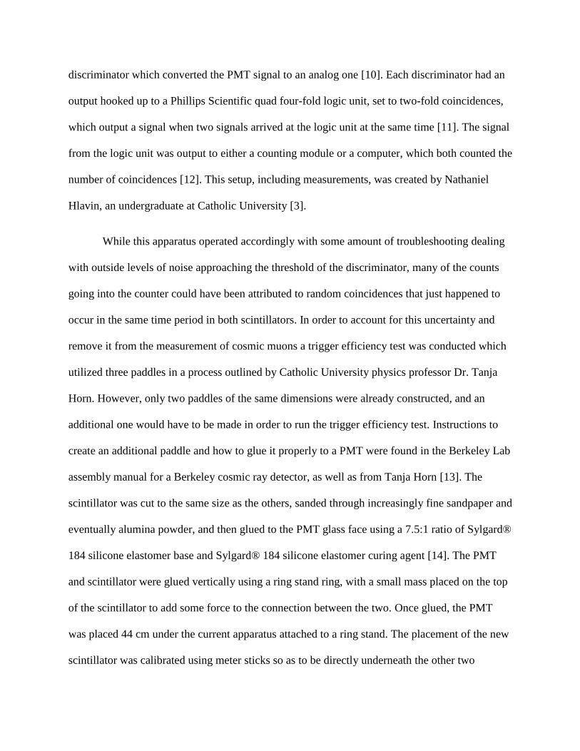
Figure 2: The x axis represents total dose the plants were exposed to across the 20 days, which included 14 exposures. The y axis represents the average change in the number of leaves from the first day of measurement to the last. The vertical uncertainty represents 1 standard deviation from the set of four or less plants. The horizontal uncertainty represents the 10% accounting for changes in the placement of the source day to day. The R
2 value represents the coefficient of determination, a
statistical value used to show the goodness of fit of the line. A value of 0 would have no statistical correlation while a value of 1 would be a perfect fit.
The x axis represents total dose the plants were exposed to across the 20 days, which included 14 exposures.
y = 2E-06x2 - 0.0039x + 5.8 R² = 0.10
0
2
4
6
8
10
12
0 500 1000 1500 2000 2500Ave
rage
ch
ange
in n
um
ber
of
leav
es o
ver
20
d
ays
(mm
)
Total Dose (μSv)
Average Change in Number of Leaves vs. Radiation Dose
Gamma
Beta
Control
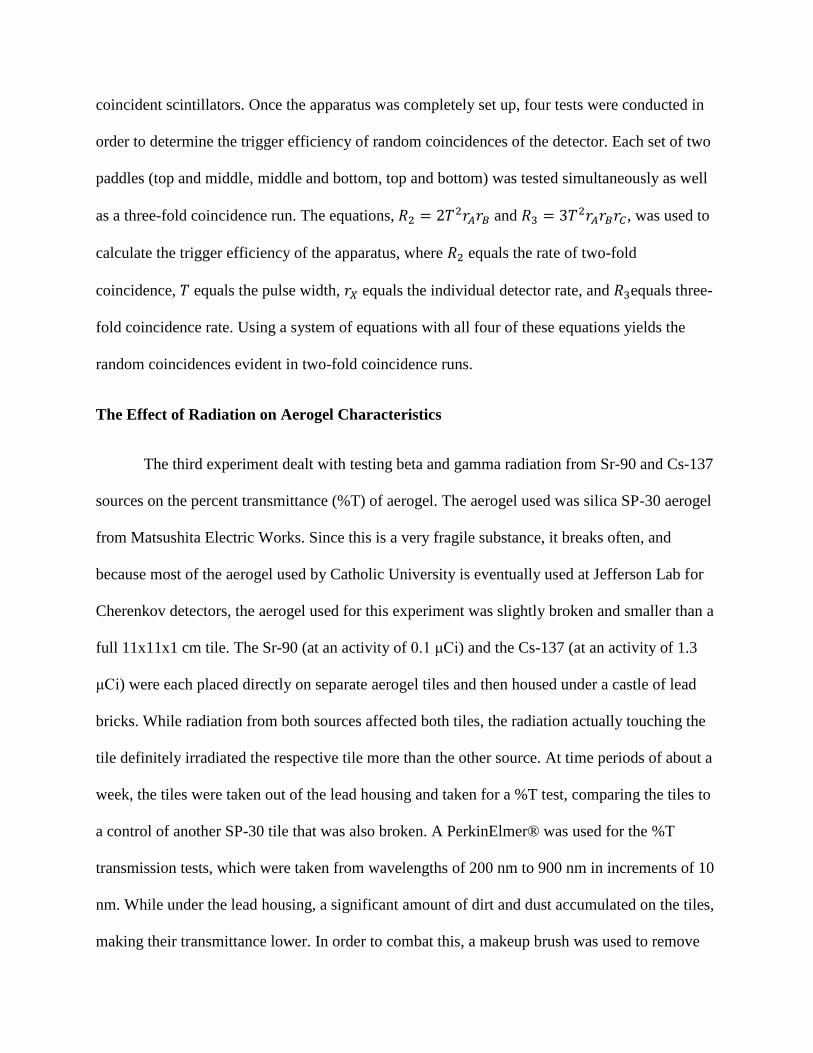
Figure 3: Time in days is displayed on the x axis while the average number of leaves for each level of independent variable at that day is displayed along the y axis. Error is derived from the standard deviation from the set of multiple repeated trials for each level of independent variable.
-2
0
2
4
6
8
10
12
14
1 2 3 4 5 6 7 8 9 10 11 12 13
Nu
mb
er
of
Leav
es
Time (days)
Number of Leaves vs Time
Control
95 Gamma
121 Gamma
224 Gamma
281 Gamma
266 Beta
339 Beta
748 Beta
1820 Beta
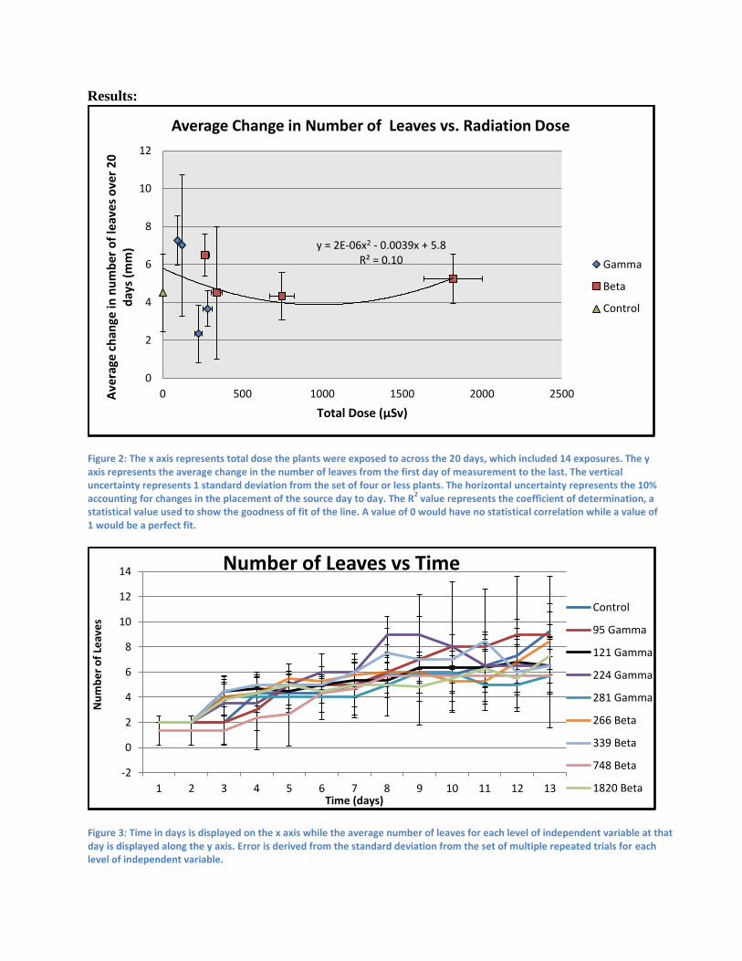
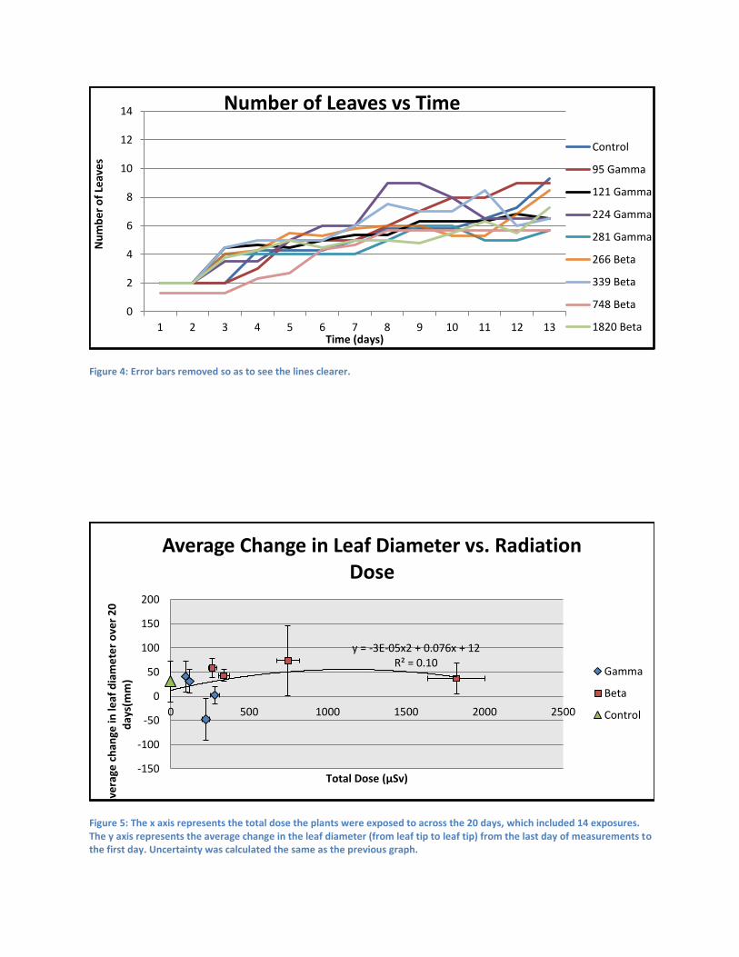
Figure 5: The x axis represents the total dose the plants were exposed to across the 20 days, which included 14 exposures. The y axis represents the average change in the leaf diameter (from leaf tip to leaf tip) from the last day of measurements to the first day. Uncertainty was calculated the same as the previous graph.
y = -3E-05x2 + 0.076x + 12 R² = 0.10
-150
-100
-50
0
50
100
150
200
0 500 1000 1500 2000 2500
Ave
rage
ch
ange
in le
af d
iam
ete
r o
ver
20
d
ays(
mm
)
Total Dose (μSv)
Average Change in Leaf Diameter vs. Radiation Dose
Gamma
Beta
Control
Figure 4: Error bars removed so as to see the lines clearer.
0
2
4
6
8
10
12
14
1 2 3 4 5 6 7 8 9 10 11 12 13
Nu
mb
er
of
Leav
es
Time (days)
Number of Leaves vs Time
Control
95 Gamma
121 Gamma
224 Gamma
281 Gamma
266 Beta
339 Beta
748 Beta
1820 Beta
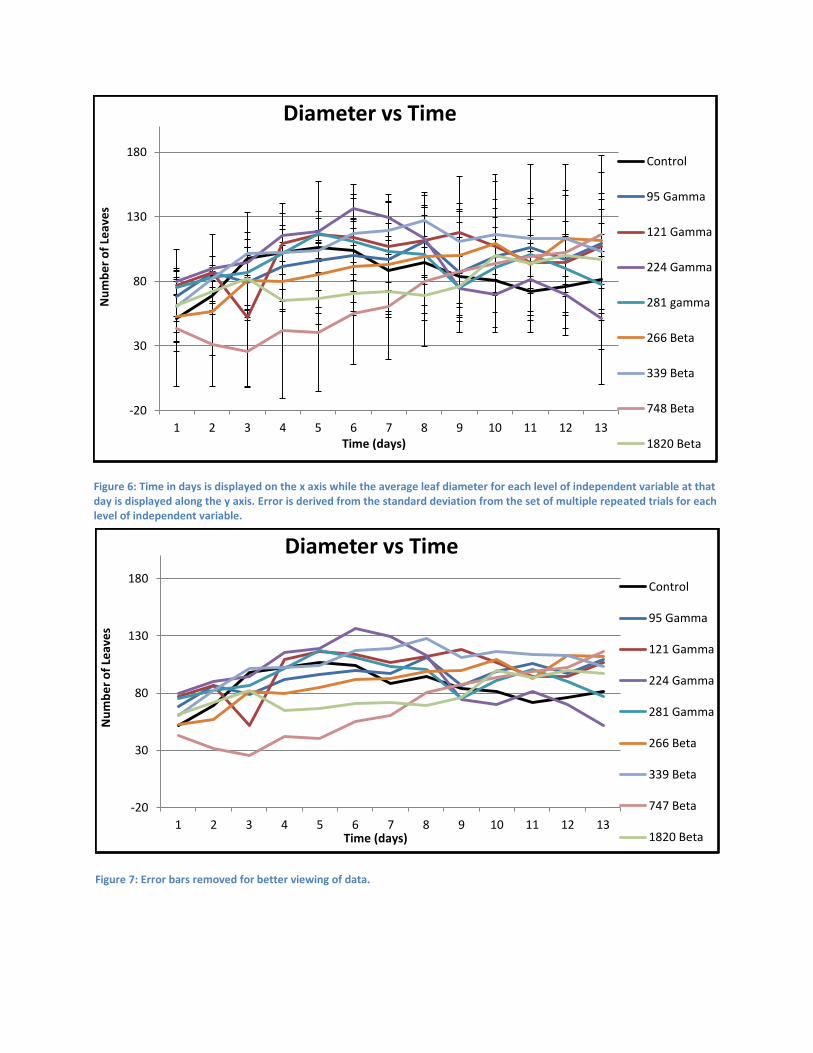
Figure 6: Time in days is displayed on the x axis while the average leaf diameter for each level of independent variable at that day is displayed along the y axis. Error is derived from the standard deviation from the set of multiple repeated trials for each level of independent variable.
-20
30
80
130
180
1 2 3 4 5 6 7 8 9 10 11 12 13
Nu
mb
er
of
Leav
es
Time (days)
Diameter vs Time
Control
95 Gamma
121 Gamma
224 Gamma
281 gamma
266 Beta
339 Beta
748 Beta
1820 Beta
Figure 7: Error bars removed for better viewing of data.
-20
30
80
130
180
1 2 3 4 5 6 7 8 9 10 11 12 13
Nu
mb
er
of
Leav
es
Time (days)
Diameter vs Time
Control
95 Gamma
121 Gamma
224 Gamma
281 Gamma
266 Beta
339 Beta
747 Beta
1820 Beta
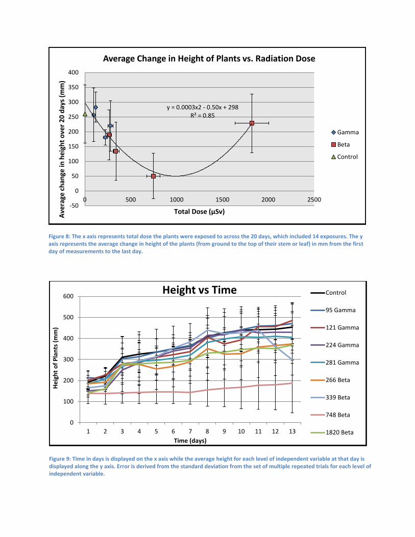
Figure 8: The x axis represents total dose the plants were exposed to across the 20 days, which included 14 exposures. The y axis represents the average change in height of the plants (from ground to the top of their stem or leaf) in mm from the first day of measurements to the last day.
y = 0.0003x2 - 0.50x + 298 R² = 0.85
-50
0
50
100
150
200
250
300
350
400
0 500 1000 1500 2000 2500
Ave
rage
ch
ange
in h
eigh
t o
ver
20
day
s (m
m)
Total Dose (μSv)
Average Change in Height of Plants vs. Radiation Dose
Gamma
Beta
Control
Figure 9: Time in days is displayed on the x axis while the average height for each level of independent variable at that day is displayed along the y axis. Error is derived from the standard deviation from the set of multiple repeated trials for each level of independent variable.
0
100
200
300
400
500
600
1 2 3 4 5 6 7 8 9 10 11 12 13
He
igh
t o
f P
lan
ts (
mm
)
Time (days)
Height vs Time Control
95 Gamma
121 Gamma
224 Gamma
281 Gamma
266 Beta
339 Beta
748 Beta
1820 Beta
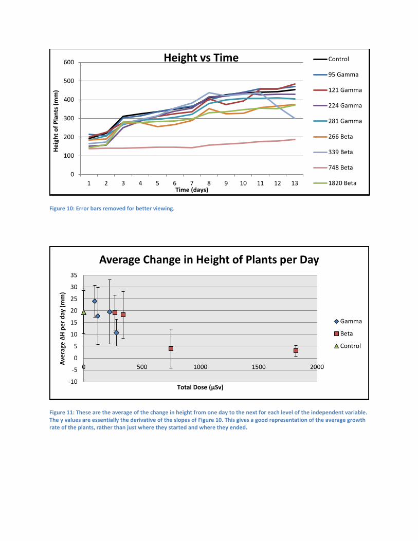
Figure 10: Error bars removed for better viewing.
0
100
200
300
400
500
600
1 2 3 4 5 6 7 8 9 10 11 12 13
He
igh
t o
f P
lan
ts (
mm
)
Time (days)
Height vs Time Control
95 Gamma
121 Gamma
224 Gamma
281 Gamma
266 Beta
339 Beta
748 Beta
1820 Beta
Figure 11: These are the average of the change in height from one day to the next for each level of the independent variable. The y values are essentially the derivative of the slopes of Figure 10. This gives a good representation of the average growth rate of the plants, rather than just where they started and where they ended.
-10
-5
0
5
10
15
20
25
30
35
0 500 1000 1500 2000
Ave
rage
ΔH
pe
r d
ay (
mm
)
Total Dose (μSv)
Average Change in Height of Plants per Day
Gamma
Beta
Control
Figure 12: The number of cells for each level of radiation is displayed for both the cortex (nearer to the outside of the cell) and the pith (close to the inside with larger cells). Error is from standard deviation from the repeated trials.
0
5
10
15
20
25
30
35
40
45
0 500 1000 1500 2000Nu
mb
er
of
cells
in o
ne
slid
e v
iew
Total Radiation Dose (μSv)
Number of Cells in Cortex and Pith
Gamma Cortex
Gamma Pith
Beta Cortex
Beta Pith
Control Cortex
Control Pith
Figure 13: This data comes from the stage Growth Experiment. The x axis represents how many weeks the plant had been germinated since the radiation began (so the one at 0 was planted the same day it began radiation treatment. Error bars come from standard deviation from each individual change, which makes them rather large as some days have little to no growth while others have a large amount of growth due to growth spurts in the plants.
-100
-50
0
50
100
150
0 0.5 1 1.5 2 2.5 3 3.5 4 4.5
Ave
rage
ΔH
eig
ht
pe
r d
ay (
mm
)
Time since germination when radiation exposure began (weeks)
Average Change in Height Per Day
Radiation
Control
Hellow there
How is it going? You can’t see this.
Isn’t that funny?
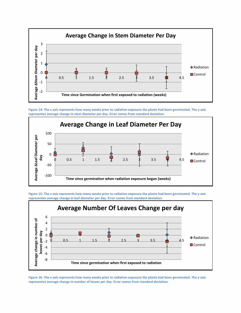
Figure 14: The x axis represents how many weeks prior to radiation exposure the plants had been germinated. The y axis representes average change in stem diameter per day. Error comes from standard deviation.
-2
-1
0
1
2
3
0 0.5 1 1.5 2 2.5 3 3.5 4 4.5
Ave
rage
ΔSt
em
Dia
me
ter
pe
r d
ay
Time since Germination when first exposed to radiation (weeks)
Average Change in Stem Diameter Per Day
Radiation
Control
Figure 15: The x axis represents how many weeks prior to radiation exposure the plants had been germinated. The y axis representes average change in leaf diameter per day. Error comes from standard deviation.
-100
-50
0
50
100
0 0.5 1 1.5 2 2.5 3 3.5 4 4.5
Ave
rage
ΔLe
af D
iam
ete
r p
er
day
Time since germination when radiation exposure began (weeks)
Average Change in Leaf Diameter Per Day
Radiation
Control
Figure 16: The x axis represents how many weeks prior to radiation exposure the plants had been germinated. The y axis representes average change in number of leaves per day. Error comes from standard deviation.
-8
-6
-4
-2
0
2
4
6
0 0.5 1 1.5 2 2.5 3 3.5 4 4.5
Ave
rage
ch
ange
in n
um
be
r o
f le
ave
s p
er
day
Time since germination when first exposed to radiation
Average Number Of Leaves Change per day
Radiation
Control
Cosmic Ray Detector Trigger Efficiency Results
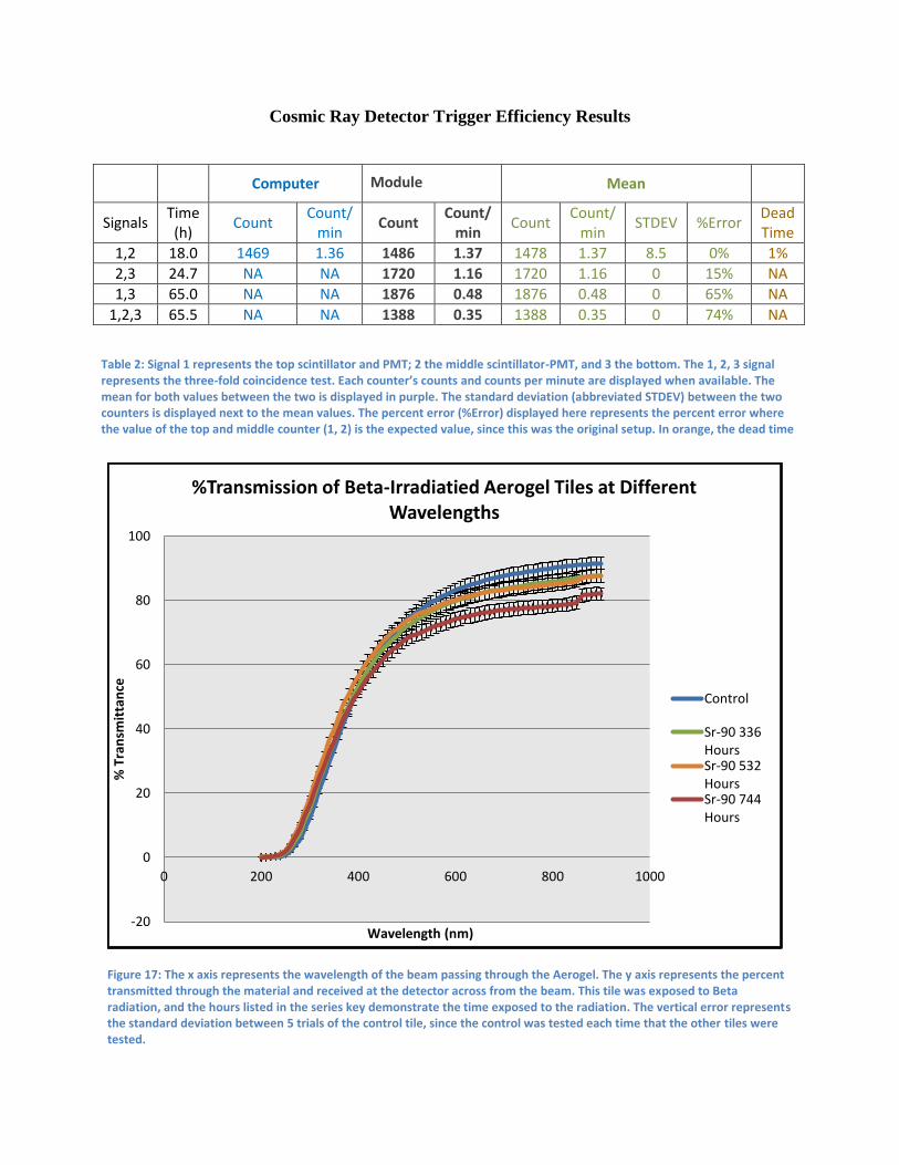
Figure 17: The x axis represents the wavelength of the beam passing through the Aerogel. The y axis represents the percent transmitted through the material and received at the detector across from the beam. This tile was exposed to Beta radiation, and the hours listed in the series key demonstrate the time exposed to the radiation. The vertical error represents the standard deviation between 5 trials of the control tile, since the control was tested each time that the other tiles were tested.
-20
0
20
40
60
80
100
0 200 400 600 800 1000
% T
ran
smit
tan
ce
Wavelength (nm)
%Transmission of Beta-Irradiatied Aerogel Tiles at Different Wavelengths
Control
Sr-90 336HoursSr-90 532HoursSr-90 744Hours
Computer Module Mean
Signals Time (h)
Count Count/
min Count
Count/ min
Count Count/
min STDEV %Error
Dead Time
1,2 18.0 1469 1.36 1486 1.37 1478 1.37 8.5 0% 1%
2,3 24.7 NA NA 1720 1.16 1720 1.16 0 15% NA
1,3 65.0 NA NA 1876 0.48 1876 0.48 0 65% NA
1,2,3 65.5 NA NA 1388 0.35 1388 0.35 0 74% NA
Table 2: Signal 1 represents the top scintillator and PMT; 2 the middle scintillator-PMT, and 3 the bottom. The 1, 2, 3 signal represents the three-fold coincidence test. Each counter’s counts and counts per minute are displayed when available. The mean for both values between the two is displayed in purple. The standard deviation (abbreviated STDEV) between the two counters is displayed next to the mean values. The percent error (%Error) displayed here represents the percent error where the value of the top and middle counter (1, 2) is the expected value, since this was the original setup. In orange, the dead time of the computer is displayed when available (the percent of counts that the computer missed that the module picked up.
Discussion
In the experiment testing radiation on plants Figure 2, Figure 3, and Figure 4 depict data
recorded regarding the number of leaves. This measurement, if high could demonstrate healthy
growing, or if too high abnormal growth. In some cases, leaves actually fell off of the plants, as
demonstrated in the 224 µSv Gamma dose in Figure 3, and Figure 4. This occurred either
because the leaves shriveled to the point where they could not be identified as leaves any longer,
or because during a measurement the stem actually snapped due to experimenter error or an
extremely thin stem. A couple plants experienced an abnormally high amount of leaves, even
though they weren’t growing them in bolts like in the other plants. In these plants, upwards of 8
Figure 18: The x axis here represents the wavelength of the beam. The y axis represents the percent transmitted through the tiles. The vertical uncertainty represents the standard deviation of the 5 trials of the control tile which was tested every time the other tiles were tested as well.
-20
0
20
40
60
80
100
0 200 400 600 800 1000
Titl
e
Title
%Transmission of Aerogel Tiles at Different Wavelengths
Control
Cs-137 192HoursCs-137 360HoursCs-137 576Hours
leaves were sprouting where usually only 2 sprout. This could possibly be attributed to the
gamma radiation that this plant was exposed to, but it also could be due to random change.
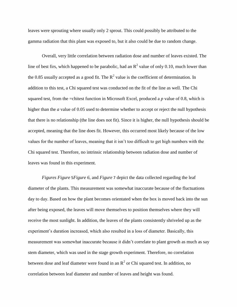
Overall, very little correlation between radiation dose and number of leaves existed. The
line of best firs, which happened to be parabolic, had an R2 value of only 0.10, much lower than
the 0.85 usually accepted as a good fit. The R2 value is the coefficient of determination. In
addition to this test, a Chi squared test was conducted on the fit of the line as well. The Chi
squared test, from the =chitest function in Microsoft Excel, produced a p value of 0.8, which is
higher than the a value of 0.05 used to determine whether to accept or reject the null hypothesis
that there is no relationship (the line does not fit). Since it is higher, the null hypothesis should be
accepted, meaning that the line does fit. However, this occurred most likely because of the low
values for the number of leaves, meaning that it isn’t too difficult to get high numbers with the
Chi squared test. Therefore, no intrinsic relationship between radiation dose and number of
leaves was found in this experiment.
Figures Figure 5Figure 6, and Figure 7 depict the data collected regarding the leaf
diameter of the plants. This measurement was somewhat inaccurate because of the fluctuations
day to day. Based on how the plant becomes orientated when the box is moved back into the sun
after being exposed, the leaves will move themselves to position themselves where they will
receive the most sunlight. In addition, the leaves of the plants consistently shriveled up as the
experiment’s duration increased, which also resulted in a loss of diameter. Basically, this
measurement was somewhat inaccurate because it didn’t correlate to plant growth as much as say
stem diameter, which was used in the stage growth experiment. Therefore, no correlation
between dose and leaf diameter were found in an R2 or Chi squared test. In addition, no
correlation between leaf diameter and number of leaves and height was found.
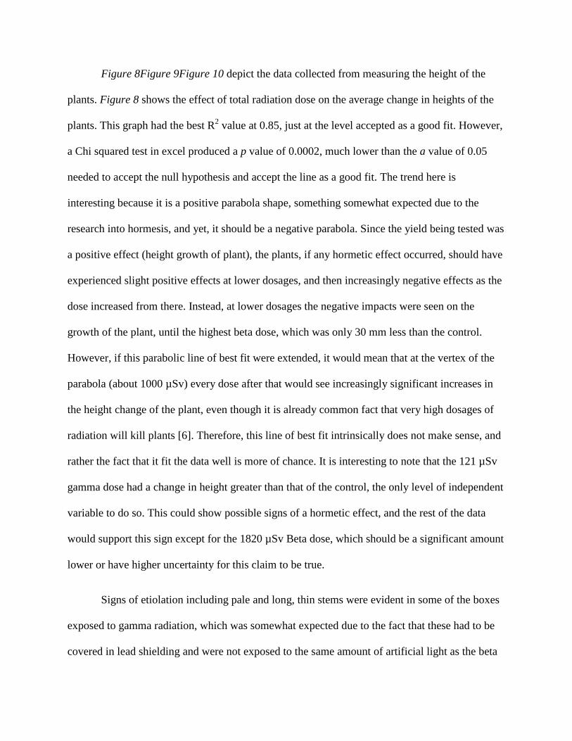
Figure 8Figure 9Figure 10 depict the data collected from measuring the height of the
plants. Figure 8 shows the effect of total radiation dose on the average change in heights of the
plants. This graph had the best R2 value at 0.85, just at the level accepted as a good fit. However,
a Chi squared test in excel produced a p value of 0.0002, much lower than the a value of 0.05
needed to accept the null hypothesis and accept the line as a good fit. The trend here is
interesting because it is a positive parabola shape, something somewhat expected due to the
research into hormesis, and yet, it should be a negative parabola. Since the yield being tested was
a positive effect (height growth of plant), the plants, if any hormetic effect occurred, should have
experienced slight positive effects at lower dosages, and then increasingly negative effects as the
dose increased from there. Instead, at lower dosages the negative impacts were seen on the
growth of the plant, until the highest beta dose, which was only 30 mm less than the control.
However, if this parabolic line of best fit were extended, it would mean that at the vertex of the
parabola (about 1000 µSv) every dose after that would see increasingly significant increases in
the height change of the plant, even though it is already common fact that very high dosages of
radiation will kill plants [6]. Therefore, this line of best fit intrinsically does not make sense, and
rather the fact that it fit the data well is more of chance. It is interesting to note that the 121 µSv
gamma dose had a change in height greater than that of the control, the only level of independent
variable to do so. This could show possible signs of a hormetic effect, and the rest of the data
would support this sign except for the 1820 µSv Beta dose, which should be a significant amount
lower or have higher uncertainty for this claim to be true.
Signs of etiolation including pale and long, thin stems were evident in some of the boxes
exposed to gamma radiation, which was somewhat expected due to the fact that these had to be
covered in lead shielding and were not exposed to the same amount of artificial light as the beta
or control boxes which received some light through the plastic, or from other means, as the
control was put under a desk in semi-darkness.
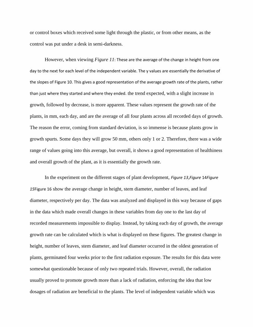
However, when viewing Figure 11: These are the average of the change in height from one
day to the next for each level of the independent variable. The y values are essentially the derivative of
the slopes of Figure 10. This gives a good representation of the average growth rate of the plants, rather
than just where they started and where they ended. the trend expected, with a slight increase in
growth, followed by decrease, is more apparent. These values represent the growth rate of the
plants, in mm, each day, and are the average of all four plants across all recorded days of growth.
The reason the error, coming from standard deviation, is so immense is because plants grow in
growth spurts. Some days they will grow 50 mm, others only 1 or 2. Therefore, there was a wide
range of values going into this average, but overall, it shows a good representation of healthiness
and overall growth of the plant, as it is essentially the growth rate.
In the experiment on the different stages of plant development, Figure 13,Figure 14Figure
15Figure 16 show the average change in height, stem diameter, number of leaves, and leaf
diameter, respectively per day. The data was analyzed and displayed in this way because of gaps
in the data which made overall changes in these variables from day one to the last day of
recorded measurements impossible to display. Instead, by taking each day of growth, the average
growth rate can be calculated which is what is displayed on these figures. The greatest change in
height, number of leaves, stem diameter, and leaf diameter occurred in the oldest generation of
plants, germinated four weeks prior to the first radiation exposure. The results for this data were
somewhat questionable because of only two repeated trials. However, overall, the radiation
usually proved to promote growth more than a lack of radiation, enforcing the idea that low
dosages of radiation are beneficial to the plants. The level of independent variable which was
planted the same day that it began being exposed to radiation also experienced significant
changes between the irradiated sample, and the non-irradiated one. In the irradiated sample, the
plants grew to heights of 84 mm and 176 mm, while the non-irradiated sample’s plants only
grew only 10 and 3 mm. This shows that the radiation could have possibly expedited the time
needed for the plants to begin growing above soil.
For the trigger efficiency test, the equation was used to calculate the
individual detector rates by setting up a system of equations using the three two-fold coincidence
tests. Then the equation, was used to calculate the expected rate of three-fold
coincidence. The value calculated was 6.27 x 10⁻⁷
ms-1
. The experimental value was 5.83 x 10⁻⁶
ms-1
, which means that the experimental was higher than the calculated, which is expected
because the experimental rate still had real counts in it as well. The paddlel efficiency was
calculated using the equation ( ) ( )
( ) , which gave the value of 0.999, an exceptional paddle efficiency.
For the experiment of radiation on aerogel transmittance, no effect outside of the
calculated standard deviation of the five control tiles was to be found in the tile exposed to
gamma radiation by Cs-137. Moreover, the transmittance did not change significantly the
different times it was tested, meaning that the transmittance did not change as the duration of
exposure increased. The most recent beta Sr-90 exposed tile however, where it was exposed for
774 hours, did see noticeable changes outside of one standard deviation from the control, and
even the other Sr-90 trials. This occurred especially at higher wavelengths. Therefore, the results
support the statement that as exposure to beta radiation increases, percent transmittance in
aerogel decreases. This possibly occurred in beta and not gamma radiation because gamma
would pass through the aerogel with more ease as it has higher energy particles, but the beta
radiation, having lower energy would be stopped more easily by the aerogel, which could cause
it to damage the tile.
Conclusion
In this experiment, different levels of ionizing beta and gamma radiation were applied to
Phaseolus vulgaris, and the results on the plants’ height, number of leaves, and leaf diameter
were recorded. Results showed some amount of a hormetic effect occurring in the lower gamma
dosages with regards to height, but overall the data proved to be rather imprecise due to not
enough trials. In the future, many more trials would have to be conducted for truly conclusive
results to be found, but nonetheless, the data does hint that some level of hormesis occurred.
With more trials, a true Gaussian curve could be used to model the plants different traits, which
in turn could lead to more interesting statistical calculations such as T-tests that could not be
used with the current test because of a lack of trials.
In addition, the effects of gamma radiation on stage growth experiment supported that
idea of a hormetic response to radiation as almost all of the stages of growth from 0 to 4 weeks
old had healthier and faster growing plants in the irradiated samples. It is especially interesting
that the irradiated plants that were planted the same day as the first radiation dose was applied
broke the soil line and began growing at a much faster rate than the plants not exposed to gamma
radiation.
Overall, there are many ways that both these experiments could have been conducted to
yield more precise and conclusive results. Besides simply more trials, the plants were grown in a
way that hindered their growth rather than allowed them to burgeon. Bean plants generally
require some sort of post in order to grow as they grow up it in vine-like spiral patterns. In fact,
some of the plants actually latched on to other plants in attempts to grow further, and these plants
did significantly better than plants with no supports. Therefore, if this experiment were done
again, some sort of stalk would be used in order for the bean plants to grow upwards, instead of
curving around looking for a support. Moreover, the boxes used for the initial dose vs. growth
experiment had plastic bags on the bottom so that the cardboard boxes wouldn’t disintegrate
from the water. However, this caused the water to stay in the box, sometimes even above soil
level, for days at a time. This caused the watering cycle to be somewhat sporadic and varied as
too much water was given to the plants in the beginning. However the amount of water each box
received stayed the same, so even though the excess water could have hurt the plants, it was a
controlled variable. In terms of controlling other variables however, the light each box received
could have been controlled in a more accurate way. The plants were exposed to radiation from
either 10:00 am to 1:00 pm or 1:00 pm to 4:00 pm, which just so happen to be the hours when
sunlight is the strongest in the geographic area the beans were planted in. Therefore, the plants
missed the light when it was the most essential for them. Furthermore, the boxes exposed to
gamma radiation required lead shielding, which made them lose even more light than the control
box or the beta box. In the future, more light should be given to the plants in order for them to
grow better, and the same amount of light should be given to each level. In addition the stem
diameter was not measured in the dose vs. growth experiment, while it was measured in the
stages of growth experiment. In the future, this measurement should be included in both as it
links to the amount of nutrients the plant is receiving from the soil.
The cosmic ray trigger efficiency, which attempted to determine the number of random
coincidences that are not muons, yielded strange results as the final trigger efficiency
calculations supported the claim that the random coincidences were occurring more frequently in
the three-fold coincidence test rather than the two fold-coincidence ones. This seems rather
unlikely as with a third detector, the solid angle of the detectors decreases and therefore the
number of random coincidences should be declining as well. It is possible that a low two-fold
coincidence rate caused this problem.
In the future, besides fixing the one two-fold coincidence count, longer trials could be
used to ensure a more accurate rate. In addition, delay tests where the discriminator or the cables
are altered so that the signals are not going into the logic unit at the same time could be
conducted in order to see if any coincidences still occur. If any coincidences do occur, these
would be purely random coincidences, not caused by muons .This value could be compared to
the calculated random coincidence rate using the paddle efficiency equation listed in the
discussion.
The effect of beta and gamma radiation on aerogel tested those two types of radiation on
aerogel tiles’ percent transmittance using a photo spectrometer. Although the results from the
gamma radiation test showed no definitive change in transmittance over time, or varying from
the control, the beta tiles’ percent transmission actually decreased significantly as exposure time
increased, and in fact varied from the control over one standard deviation. Therefore, the results
support the claim that beta radiation causes percent transmittance to decrease in aerogel tiles.
If the experiment were to be done again, further safeguards should be used to ensure that
dust and debris do not infect the tiles while they are under lead shielding exposed to radiation.
This could have skewed the data to have lower percent transmittances than expected. In fact, it is
possible that this problem is what caused the most recent beta percent transmittance test to differ
significantly from the other trials, however, it differs by such a significant amount, that this is not
likely.
Works Cited
1 United State Environmental Protection Agency. Radiation: Non-Ionizing and Ionizing. Radiation
Protection [Internet]. 2013 April 17. Available from: