The Effect of Lake Temperatures and Emissions on Ozone ... · The Effect of Lake Temperatures and...

J O U R N A L O F A P P L I E D M E T E O R O L O G Y

The Effect of Lake Temperatures and Emissions on Ozone Exposure in the Western Great Lakes Region

Pacific Norihn~est Nhtional Laboratory, Richland, Washingon

North Central Research Sfation, USDA Forest Service, East Lansing, Michigan

(Manuscript received 8 August 2002, in final fonn 12 December 2002)

ABSTRACT

A meteorological-chemical model with a 12-km horizontal grid spacing was used to simulate the evolution of ozone over the western Great Lakes region during a 30-day period in the summer of 1999. Lake temperatures in the model were based on analyses derived from daily satellite measurements. The model performance was evaluated using operational surface and u.er-air meteorological measurements and surfsce chemical measurements. Reasonable agreement between the simulations and observations was obtained. The bias (predicted - observed) over the simulation period was only - 1+3 ppb for the peak ozone mixifig ratio during the day and 5.5 ppb for the minimum ozone mixing ratio at night. tfigh ozone production rates were produced over the surface of the lakes as a result of stable atmospheric conditions that trapped ozone precursors within a shallow layer during the day. In one location, an increase of 200 ppb of ozone over a 9-h period was produced by chemical production that was offset by losses of I10 ppb through vertical mixing, horizontal transport, and deposition. The predicted ozone was also sensitive to lake temperatures. A simulation with climatological lake temperatures produced ozone mixing ratios over the lakes and around the lake shores that differed fkom the simulation with observed fake temperatures by as much as 50 ppb, while the differences o v a land were usually 10 ppb or less. Through a series of sensitivity studies that varied ozone precursor emissions, it was shown that a reduction of 50% in NO, or volatile organic compounds would lower the 60-ppb ozone exposure by up to 50 h month-' in the remote forest regions over the northern Great Lakes. The implications of these results on future climate change and air quality in the region are discussed.

1. Introduction and to increase dark respiration in a stand of sugar maple

In addition to the effects of ozone on human health (McKee 1994), it is well-known that high surface ozone concentrations can have an adverse effect on many different types of vegetation in the upper Great Lakes region. For example, Colman et al. f 1995) examined the effects of ozone exposure on various aspen (Populus tremuloides) clones in northern Michigan. Whole-tree photosynthesis was found to decrease in all. clones in response to enhanced ozone concentrations, along with earfy leaf abscission. A 5-yr study by Kamosky et at. (1993) found varying degrees of sensitivity to seasonal ozone exposure on growth, physiology, and carbon al- location for three different types rrf tree species (Aceu sacchamrn, Pinus strobus, and Populus tremuloides). Ozone was found by Tjoefker et a1. (1995) to reduce net photosynthesis in light-saturated areas of the canopy

Corresponding author address: Jerome Fast, Pacific Northwest Na- tional Laboratory, P.O. Box 999, K9-30, 3200 Q Avenue, Richland, WA 99352.. E-mail: [email protected]

(Acer sacchamrn). Other studies of the effects of ozone _on vegetation common in the western Great Lakes region have been performed by Wang et al. (1986), Ar- mentano and Menges (1987), Bennett et af. (1992, 1994), Volin et al. (1993), Reich et al. (1990), and Re- zabek et al. (1989).

These studies have filled a gap in wt- undersbnding of the importance of vegetationlozone interactions, but information is also needed on the relevant photochemical processes t a t lead ta high surface azme episades and the meteorological processes that transport ozone fkom urban areas to remote sites containing ozone-sensitive vegetation. The Lake Michigan Ozone Study (LMOS; Koerber et al. 1991) and the Program for Re- s m f ; z mz Oxidants: P b t istry, Emissions, md Transport (PROPHET; Carroll et al. 2001) are the most recent field expekents that have collected meteorological and chemical measurements in the region.

LMOS was an air quality field campaign, conducted over a 7-week period during the summer of 1991, in which measurments were made by surface monitoring

Q 2003 American Meteorological Society 1197

1198 J O U R N A L O F A P P L I E D M E T E O R O L O G Y V O L ~ 42

FIG. 1. Time series of daily maximum ozone in the vicinity of Lake Michigan at eight ozone monitoring stations during Jul and Aug of 1999.

stations, aircraft, and boats. An analysis of the observations by Dye et al. (1995) revealed that the highest pzone concentrations occurred in a shallow cool layer adjacent to Lake Michigan and were subsequently transported to the shores of Wisconsin and Michigan. Sillman et al. (1993) showed that suppressed vertical mixing and deposition in a model were needed to produce high ozone concentrations over the lake. Several mesoscale modeling studies have been performed to evaluate their ability to simulate lake-breeze circulations (Eastman et al, 1995) and to assess how local circulations could influence ozone transport (Lyons et al. 1995; Hanna and Yang 2001; Shafran et al. 2000). Similar to previous studies of the eastern United States (e.g., Vukovich 1979 and others), meteorological analyses by Hanna and Chang (1995) and Dye et al. (1995) showed that high- ozone events in the region resulted from local sources contributing to an already polluted air mass associated with a high pressure system. Hanna et al. (1996) found that U.S. Environmental Protection Agency (EPA) reg- ulatory models underpredicted ozone and ozone precursors 200-500-km downwind of the major sources, where ozone concentrations greater than 150 ppb were observed.

In contrast with most air quality field campaigns that collect extensive data over a wide area for a short period of time, PROPHET has collected extensive chemical measurements at a single remote site in northern Mich- igan over the past several years. While PROPHET has focused on the photochemical processes within and just above the forest canopy at this rural site, it also has assessed the role of transport processes and the impact of upwind anthropogenic and biogenic emissions in the Wdwest. For example, meteorological analyses and back trajectories indicated that changes in the local chemistry could be explained by rapid and frequent tran- sitions between clean Canadian air and regions of higher mthropogentic emissions in the United States (Cooper et al. 2001).

In this study, we employ a coupled meteorological and chemical model to simulate the evolution of ozone in the western Great Lakes region over a 30-day period. Because the lakes compose a large fkaction of the surface area of the region, the effect of lake temperatures on the production of ozone will be quantified. To examine how ozone concentrations and ozone exposure are affected by local pollutant sources, a series of sensitivity simulations a& performed that vary ozone precursor emission rates. This study is also intended to be a first step toward determining future ozone exposure patterns resulting from regional-scale landscape change predictions; therefore, the implications of the findings on factors needed to be accounted for by climate chemistry models will be discussed.

2. Model description and experimental design

A coupled meteorological and chemical modeling system is employed to simulate the production/destruction, turbulent mixing, transport, and deposition of ozone over the western Great Lakes region. A 30-day period between 15 July and 14 August 1999 was simulated. This period was chosen because there were days with both high and low ozone concentrations over the Great Lakes region, as shown in Fig. 1. This allowed for the investigation of the efFects of emission rates and lake temperatures on ozone concentrations for a variety of meteorological conditions. Clinzatologieal studies have shown that high-ozone episodes in the eastern United States often occur along the back sides of slow- moving, persistent Bermuda high pressure systems (e.g., Vukovich 1995). During July of 1999, there were several periods in which the meteorological conditions were conducive to local ozone production and regional-scale ozone transport into the Great Lakes region. After 1 August, howevet, the daily peak ozone mixing ratios were lower because the region was under the influence of a series of continental high pressure systems.

F A S T A N D H E I L M A N 1199

FIG. 2. Dominant vegetation types with the [(a): left panel] second and [(b): right panel] third modeling domains: crop (light green), grass (medium green), forest (dark green), and &an (red). N W S rawinsonde stations (yellow dots) in the western Great Lakes region are shown in (a) and EPA ozone monitoring stations are shown in (b). In (b), surface lake temperatures (red contours) on 15 Jul 1999 and the locations of meteorological stations (white dots) described in the text are shown.

The Northeast Oxidant and Particulate Study (NE- OPS) field campaign (Philbrick et al, 2002) took place during this 30-day period so that additional surface and upper-air meteorological and chemical measurements could be used to evaluate results in a portion of the modeling domain. While the NE-OPS field campaign took place in the vicinity of Philadelphia, Pennsylvania, downwind of the Great Lakes region, the chemistry data aloft provide critical information needed to evaluate how well the model simulates regional-scale transport of pollutants from upwind sources. A complete description of the model, the Pacific Northwest National Lab- oratory (PNNL) Eulerian Gas and Aerosol Scalable Uni- fied System (PEGASUS), and its application to the NE- OPS field campaign is given in Fast et al. (2002); therefore, we briefly describe next only the details relevant to the present study.

a. Meteorological model

Version 4.3 of the Regional Atmospheric Modeling System (RAMS) mesoscale model (Pielke et al. 1992) was used to simulate the meteorological conditions between 1200 UTC 15 July and 1200 UTC 14 August. RAMS employs a two-way interactive nested grid structure, and in this study the model domain consisted of three domains. The first domain included most of eastern North America, with a grid spacing of 48 krn. The second domain, shown in Fig. 2, encompassed the north- central and northeastern United States and southern Canada, with a 24-km grid spacing, while the third domain encompassed the western Great Lakes, with a 12- km grid spacing. A terrain-following coordinate system was used with a vertical grid spacing of 25 m adjacent to the surface, which gradually increased to 600 m near

the model top at 20 km. Because of the staggered vertical coordinate, the first grid point was 12.5 m AGL.

The turbulence parameterization consists of a sim- plified second-order closure method that employs a prognostic turbulence kinetic energy equation (Mellor and Yamada 1982; Helfand and Labraga 1988). A cumulus parameterization was activated to produce cloud water and precipitation. The shortwave and longwave parameterizations include cloud eEects to determine the heating or cooling caused by radiative flux divergences. Prognostic soil-vegetation relationships were used to calculate the diurnal variations of temperature and moisture at the ground-atmosphere interface. The distribution of the dominant vegetation categories (crop, grass, forest, and urban) is shown in Fig. 2. Soil moisture was initialized using values obtained from the National Cen- ters for Environmental Prediction's Aviation ( A m ) Model. Turbulent sensible heat, latent heat, and mo- mentum flues in the surface layer were calculated fiom similarity equations. Lake temperatures in the model varied linearly in time, based on the National Oceanic and Atmospheric Administration's (NOAA) Great Lakes Environmental Research Laboratory (GLERL) daily analyses derived ftom satellite data. The analyses, which employ a horizontal grid spacing of about 3 km, were averaged to the 12-km grid, and the initial values on 15 July 1999 are shown in Fig. 2b.

Application of a four-dimensional data assimilation (4DDA) technique (Fast 1995) was necessary to limit the forecast errors in the meteorological fields over the long simulation period. In this study, 4DDA nudged the horizontal u and v components of the wind, potential temperature, and humidity into closer agreement with the 6-h analyses fiom the AVN model. A relaxation coefficient of 4.6 X s-I was used. While the stan-

1200 J O U R N A L O F A P P L I E D M E T E O R O L O G Y VOLUME 42

(a) NOx emission rates fbl isotxene emission rates

i o x 1d4md ca%'

Fro. 3. Emissions of (a) NO, and (b) isopx

1 2 5 10 20 50 7 0 0 2 0 0 S O C l O O D

$.ox i d P ~ a n z s i

me on grid 3 at 1800 UTC 15 Jul 1999.

dard upper-air soundings at 0000 and 1200 UTC, such the large-scale cloud fields was reflected in modifica- as the soundings at Green Bay, Wisconsin, and Alpena tions to the vertical velocity and turbulent kinetic energy and Detroit, Michigan, shown in Fig. 2, are not included (and, thus, eddy diffusivity) fields. Thus, large-scale directly by 4DDA, they are included indirectly through cloud mixing was included, but subgrid cloud mixing the large-scale analyses. (e.g., fair weather cumulus) was not. Photolysis rates

were modified by clouds, similar to Chang (1987), using

b. Chemical transport model

The Eulerian chemical transport model includes emission, transport, vertical diffusion, chemical produetid destruction, and dry deposition terms. The gas-phase chemistry in PEGASUS is modeled with the Carbon Bond Mechanim (CBM)-2, (Zaveri and Peters 1999) that contains 53 species and 133 reactions. CBM-Z employs the lumped-shucture approach for cmdmsing organic species and reactions, and is based on the widely used version IV (CBM-IV) developed by Gery et al. (1 989) for use in u r b ~ airshed models.

The domain for the chemical model coincided with the RAMS nested grids shown in Fig. 2. W l e the meteorological grid extended up to 20 km AGL, chemistry was simulated up to 6 h AGL. Hourly meteorological fields (h.izmtaf and vertical wind c o m p nents, temperature, humidity, eddy diffusivity, fractional area cloud coverage, and surface properties) were obtained Erorn. the msoscaln, model. The initial and lateral boundary conditions for the Great Lakes domain (Fig. 2b) were obtained from grid 2 (Fig. 2a). For grid 2, the initial, lateral, and top boundary conditions for ozone were based on climatological and observed ozo- nesonde profiles. The initial conditions for the other trace gas species on grid 2 were assigned low back- ground values and were held constant during the simulation period. The associated mixing of trace gases with

the fractional area cloud coverage. H a d y emission rates ctf 14 species were cthtaiaed

from the Sparse Matrix Operator Kernel Emissions fSh/fOKE) model CHouyoux et al. 20001. For this study, the emissions were based on the meteorological conditions from the RAMS simulation that varied hourly over the 30-day period-. The SMOKX emissions were generated of3ine on a 4-km grid over the eastern United States and Canada, using RAMS meteorological values interpolated to; the 4 - h ~ grid. Tfre emissions wese then aggregated to the 12-km grid spacing used by the PEG- ASUS simulation. The NO, [sum of nitric oxide (NC)) and nitragen dioxide (NO,)] and isoprene emissians at 1800 UTC 15 July, a Thursday, are shown in Fig, 3 to illustrate the spatial distribution over the Great Lakes modeling domain. Emissions were vertically resolved by SMOKE for the lowest eight layers of PEGASUS. Emissions above the first layer are primarlfy from point sources, such as those from power plant stacks. The highest NO, emission rates occurred over urban areas. A few point sources with high emission rates are located in rural areas along the shores of Lake Superior and Lake Huron. The highest isoprene emission rates occurred in Canada, northern Michigan, and northern Wis- consin, where forest vegetation types dominate (Fig. Zb), while low isoprene emission occurred over crop areas.

S w m m 2003 F A S T A N D H E I L M A N

360 - p 270 0 5 leo - g w

0

8 10 12 14 16 l8 20 22 24 26 28 30 1 3 5 7 9 I f 13 15

JUty date (UTC) Aupst

FIG. 4. Time series of observed (dots) and simulated (lines) temperature, wind speed, and wind direction for (a) Lansing, MI, and (b) moored buoy 45007.

We first present a comparison of the observed and simulated meteorological and chemical values during the 30-day period. The model run described in the previous section is referred to as the control simulah'on. The results of a series of sensitivity ssinulatims are then presented in section 4 to examine the effect of lake temperature and emission rates on ozone exposure in the region,

in southern Lake Michigan (Fig. 2b), is shown in Fig. 4. For Lansing (Fig. 4a), the model reproduced the magnitude and mdtiday variation rrf the maximum surface temperature well. The simulated nighttime minimum temperatures were usually 1"3"C too high after 23 July, except for a few nights that were 3"-9"C too high. This warm nighttime bias is probably due to vertical reso- lution hr the model. Because the first grid ponrt was 12.5 m AGL and the observations were at 2 m AGL, strong stratification within the nocturnal boundary layer would not be adequately represented by the model. For

a. Bounda~y layer properties example, a preliminary simulation with a 50-m vertical The simulated meteorological fields were compared @d spacing at the surface produced nightthe temper-

with surface obsavations over the model domain and atures higher than those shown in Fig. 4a. The predicted of wind, temperature, and humidity from the wind speeds and directions were s d a r to the obser-

standard rawinsonde profiles at 0000 and 1200 UTG. vations, except that the simulated peak wind speeds dur- An example of the observed and predicted surface q u a - ing the afternoon were too low on most days. tities for Lansing, Michigan and buoy 45007, located Over the lake (Fig. 4b), the diurnal variation in tem-


TABLE 1. Bias and correlation coefficient for the hourly temperahire, wind speed, and wind direction over the 30-day simulation period at the two surface stations shown in Fig. 4. All the biases are s~tistically significant using a Student's t test with a = 0.05.

Bias (model - observed) Correlation coefficient

Temperawe S-PW~ Direction Temperature Speed Direction cOcl (m s-') ("1 ("C) (m s-'1 (")

Lansing 1.91 -0.76 -4.47 0.83 0.69 0-79 Buoy 45007 0.70 - 1.00 2.30 0.78 0.52 0.82

perature was much less than over land, and the simulated temperatures were close to the observed. This was not surprising because the lower boundary condition in the model employs the observed temperature dis~bution derived from satellite data. The simulated diurnal variation in temperature, howevel; was out of phase with the observations, especially between 15 and 19 July. This may be partly due to satellite measurements that were not necessarily made at the same time each day and the linear interpolation of the lake temperatures from day to day. The performance of the model in sim- ulating the winds over the lake was similar to Lansing (Fig. 4a), except that the model did not capture as much of the wind direction variance during the period. Sig- nificantly higher wind speeds were produced over the lake because of the smaller roughness, but, as with land stations, the peak wind speeds in the afternoon were underpredicted.

Statistics that quantify the overall errors associated with the simulated surface temperature, wind speed, and direction shown in Fig. 4 are given in Table 1. While the magnitudes of the biases over land and water were somewhat different, the temperatures at night were too high, wind speeds were too low, and wind directions were too westerly for both areas. The correlation coefficients for temperature and wind direction were between 0.78 and 0.83, indicating that the model produced much of the observed variance during the 30-day period. However, the lower correlation coefficients for wind speed were largely due to predicted peak wind speeds that were too low, as indicated by the time series in Fig. 4. The model performance at other sites located within the inner grid was similar to the values in Table 1.

A number of factors may contribute to the underprediction of the peak wind speeds. For example, the current vertical grid spacing may not be adequate to resolve strong near-surface vertical wind shears. Rough- ness lengths employed by the surface parameterization may be too large as well. Over the lake, the differences in the observed and simulated winds, such as those in Fig. 4b, will produce pollutant-transport errors because the shallow stable layer is decoupled from the air aloft most of the day. Over land, diRerences between the observed and simulated wind, such as those in Fig. 4a, become less of a factor because wind speed errors aloft were small and regional-scale transport of pollutants occurs in a deep layer during the daytime convective boundary layer.

The winds aloft were evaluated by comparing the simulated results with the 0000 and 1200 UTC rawinsonde winds that were not directly employed by 4DDA. A time series of wind speed, direction, temperature, and relative humidity at the Alpena site (Fig. 2a) at about 770 m AGL is given in Fig. 5. This level was chosen because it was usually located in the middle of the afternoon convective boundary layer. Observed winds at 770 m AGL were available at each time period, but temperature and humidity were obtained by vertical interpolation &om the observed profile. Because the model employed 4DDA, the meteorological fields followed the synoptic patterns during the 30-day period and the model predicted well the observed trends in temperature, humidity, speed, and direction throughout the 30- day period. On a few days, relatively large differences occurred in the relative humidity, but there was no significant bias overall. The wind directions at Alpena and other nearby upper-air sites during the period were usually westerly or northwesterly, indicating that transport from high-pollutant sources to the south over the Ohio River valley did not occur frequently.

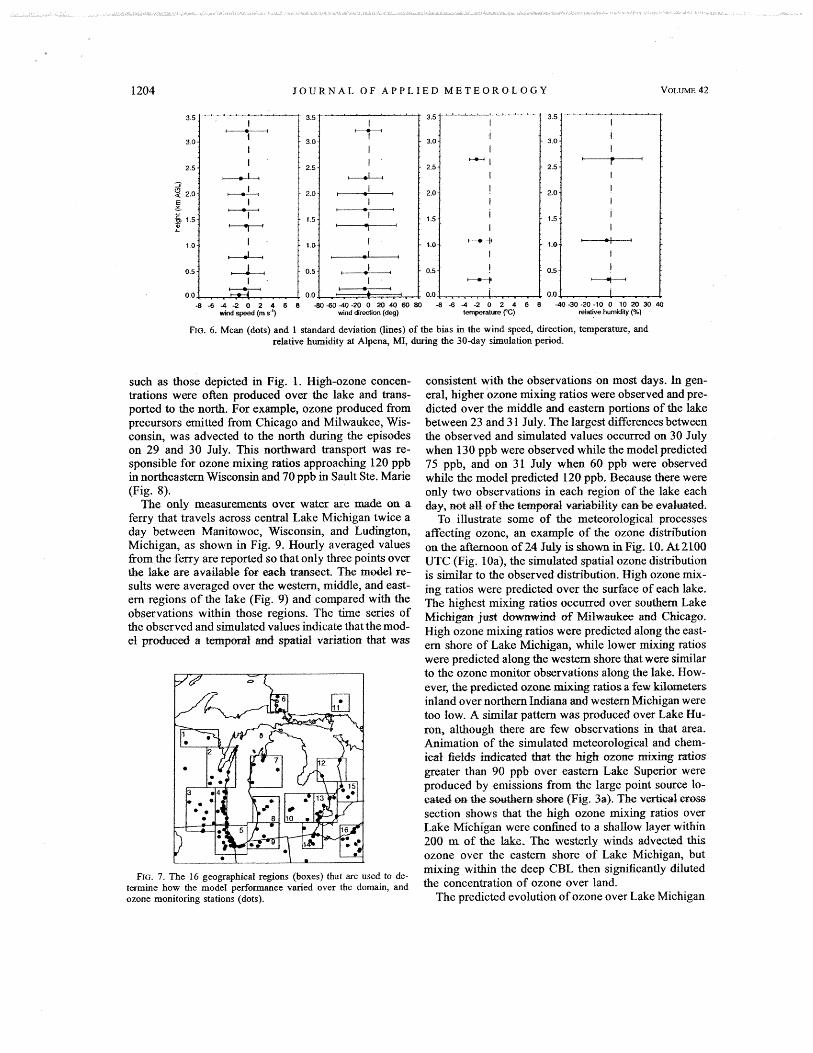
The bias, simulated - observed, in the wind speed, direction, temperature, and relative humidity within 3.5 km of the ground at Alpena is shown in Fig. 6 . On average, the model winds were slightly lower than observed between 0.2 and 1.5 km AGL and above 3 km AGL. Somewhat larger errors between 1 and 2 m s-I were produced between 1.5 and 3 km AGL. At the surface, wind speeds were 1.5 m s-' too low on average, consistent with the comparison with the surface observations (Fig. 4). While there was very little bias in the wind directions near the surface and above 2.5 km AGL, the simulated directions were usually 5O-10" different than observed between. 0.5 and 2 km AGL. Figure 5 indicates that some of the variance in Fig. 6 was associated with timing errors of a few hours or less. The overall errors for the other rawinsonde stations were similar to those shown in Fig. 6.

The parameters with the largest uncertainty in mesoscale models are usually associated with clouds. A qualitative agreement was found between the simulated spatial cloud distribution and satellite images of the observed cloud distribution thoughout the 30-day period (not shown), especiaIly when fronts were moving through the region. However; the amount of cloudiness was significantly different than that observed on some days at specific locations as expected.

S ~ ~ E R 2003 F A S T A N D H E I L M A N

-770 rn AGL AIpena Wktgan 3 3 l " ' " ' " ' " ' ~ ' " " ' " " " " " " ' " t

- 2 . . . . . . . . . . . . . . . . . . . . . . . . . . . . . , . . . . . . F

8 10 12 14 16 18 20 22 24 26 28 33 1 3 5 7 9 11 13 15

8 10 12 14 16 18 ZfJ 22 24 26 ;18 30 1 3 5 7 9 11 13 15

July date (UTC) August

Fro. 5. Time series of observed (dots) and simulated (fines) temperature, relative humihity, wind speed, and wind direction at about 770 m AGL at Alpena, MI.

6. Air chemistry evolution of ozone throughout the period. The average

Because the mesoscale model reproduced the main features of the observed winds and boundary layer evolution, the chemical transport model is expected to provide a reasonable estimate of regional-scale transport of pollutants over the domain shown in Fig. 2 d&g the 30-day period. The meteorological fields in the chemical transport model were varied linearly in time with a 5- min time step, using the archived hourly output &om the mesoscale model. As discussed in section 2, the emissions that depended on the simulated meteorological fields were updated hourly.

Because of the variable surface properties in the Great Lake region (l&ake, vegetation, &ace gas emishn rates), a complex spatial distribution of ozone is expected. To determine how the model performance varied over the domain, 16 geographical regions denoted by the boxes shown in Fig. 7 were defined. These regions encompass portions of the take shore or inland areas and are also based on the proximity of an ozone-monitoring station to an urban area. For example, regions 5, 13, and 16 include statians in the viciaity af Chicago, Illinois, Detroit, and Cleveland, Ohio, respectively. In remote northern areas, a small geographic region sur- rounding a single monitoring station is used. Simulated values from grid cells located entirely over water are excluded.

A direct comparison of the observed and simulated surface ozone over the 30-day period is shown in Fig. 8 for regions 2, 6, 7, and 10. In region 2, over northeastern Wisconsin, the model reproduced the observed

maximum and minimum values were usually close to o b s a v d and the range of simuLated values encorn- passed the range of observed values. In region 6 around Sault Ste. Marie, Michigan, the multiday trend in ozone was similar to the observed, but the average simulated maximum and minimum values were somewhat too high. The range of values, however, indicates that thew were some grid cells with ozone mixing ratios similar to observations. In region 7, over northern Michigan, tfre range of values predicted by the model usually included the observations, but the diurnal variation was lower than observed because the minhum values were overestimated, Over central Michigan in region 10, both the average maximum and minimum simulated values were quite g d , with the exception of a fezw days (e.g., 26 July).

The minimum values were usually predicted better in regions 2 and 10, presumably b e c a u of NO titration at night with the relatively higher emission rates in these areas. The NO emission rates in rural areas, such as regions 6 and 7, may be too low. Another factor for the positive bias in the minimurn ozone values in rural areas may be that the mesoscale model produced too much mixing adjacent to the ground during the stable conditions at night. Because the emission rates were low, a slight overestimation in the vertical eddy diflbsivity coefficient would be sufficient to dilute NO near the ground.

The modeling system was able to capture the spatial variations in ozone on both sides of Lake Michigan,


-8 -6 -4 -2 0 2 4 6 8 -80-6040-200 20406080 % -6 -4 -2 0 2 4 6 8 40-30-20-100 10203040 wind speed (m ") wind direction (deg) tempeCatwe f'c) relative hurnidii (96)

FIG. 6. Mean (dots) and 1 standard deviation (lines) of the bias in the wind speed, direction, temperature, and relative humidity at Alpena, MI, during the 30-day simulation period.

such as those depicted in Fig. 1. High-ozone concentrations were oRen produced over the lake and transported to the north. For example, ozone produced from precursors emitted from Chicago and Milwaukee, Wis- consin, was advected to the north during the episodes on 29 and 30 July. This northward transport was re- sponsible for ozone mixing ratios approaching 120 ppb in northeastern Wisconsin and 70 ppb in Sault Ste. Marie (Fig. 8).

The only measurem.ents over water are made on a ferry that travels across central Lake Michigan twice a day between Manitowoc, Wisconsin, and Ludington, Michigan, as shown in Fig. 9. Hourly averaged values from the ferry are reported so that only three points over the lake are available fm e a ~ h trmsect. The mxk1 results were averaged over the western, middle, and eastern regions of the lake (Fig. 9) and compared with the observations within those regions. The time series of the observed and simulated values indicate that the model prod& a tenqxmli arrd sptial variation that was

consistent with the observations on most days. In gen- eral, higher ozone mixing ratios were observed and predicted over the middle and eastern portions of the lake between 23 and 3 1 July. The largest differences between the observed and simulated values occurred on 30 July when 130 ppb were observed while the model predicted 75 ppb, and on 31 July when 60 ppb were observed while the model predicted 120 ppb. Because there were only two observations in each region of the lake each day, nd all of the ternpopid l-a&+bili$y can be evalw$ed.

To illustrate some of the meteorological processes affecting ozone, an example of the ozone distriiution on the i&emooa af 24 July is shorn in Fig, 10. At 2100 UTC (Fig. lOa), the simulated spatial ozone distribution is similar to the observed distribution. High ozone mixing ratios were predicted over the surface of each lake. The highest mixing ratios occurred over southern Lake Michigan just downwind of Pc/Eilw&w and Chicago. High ozone mixing ratios were predicted along the eastern shore of Lake Michigan, while lower mixing ratios were predicted along the western shore that were similar to the ozone monitor observations along the lake. How- eve& the predicted ~zcrne &kg ratias a few UOMetas inland over northern Indiana and western Michigan were too low. A similar pattern was produced over Lake Nu- ron, although there are few observations in that area. Animation of the simulated meteorological and chem- iml fielids i n d i d tkzt tke high ozme mixing ratios greater than 90 ppb over eastern Lake Superior were produced by emissions fiom the large point source lo- wed cxl. & w & ~ = shoMz (Fig. 3a). % va-tkal cross section shows that the high ozone mixing ratios over Lake Michigan were confined to a shallow layer within 200 m of the l&, The westerly winds advected this ozone over the eastern shore of Lake Michigan, but

FIG. 7. The 16 geographi~ai regions (boxes) that are used to de- mixing within the deep CBL then significantly diluted

tennine how the model performance varied over the domain, and the Ozone Over land* ozone monitoring stations (dots). The predicted evolution of ozone over Lake Michigan

SEPTEMBER 2003 F A S T A N D H E I L M A N 1205

15 17 19 21 23 25 27 2 9 31 . ? . 4 6 . 8 , , 10 , . 12 , , 14 , . (dl120' ' . . ' . ' ram 10, central Mwcgan t

15 17 19 21 23 25 27 29 31 2 4 6 8 10 12 14 A& date (UTC) August

FIG. 8. Time series of observed and predicted ozone for regions (a) 2, (b) 6, (c) 7, and (d) 10: hourly observations (dots), simulated average (line), and simulated range (gray shading) within each region.

~ ~ ' ~ ' " " ~ ' ' ~ ' ' ~ ~ ' ~ ~ ~ ' ' ~ ~ ~ ~ a ~ ~ ~

we& Lake Mdigan

15 17 19 2t 23 25 27 29 31 2 4 S 8 10 12 14

1 5 0 ' . ' ' ' ' . ' ' ' " ' " " ' ' ' ' ' ' " ' ' ' ' ' " ' ' ' ' " '

middle Lake Mchian 1

@as! Lake M c h i n

15 13 19 21 23 25 27 29 31 2 4 6 8 10 t2 14

July date W C : Augusl

Fra. 9. Observed hourly average ozone mixing ratios obtained from measurements made on a ferry over Lake Michigan (dots) and simulated ozone (line) along the ferry transects. Observed and simulated values are averaged over western, middle, and eastern regions (boxes in the upper-right panel) and the simulated range of ozone within the boxes (gray shading). The observed vs simulated ozone for all locations is shown in the lower-right panel.

1206 J O U R N A L O F A P P L I E D M E T E O R O L O G Y VOLW 42

ta) 21 UTC 24 Julv 1999 (b100 UVC 25 Julv 1999 --+ 5 mt S"

West East East

West €as **a

40 -so t j ~ 70 rn 90 rm 1 1 0 t 2 0 p p h

on 24 July was consistent with the ferry data, as shown in Fig. 1 I, except during the late afternoon. While the observed and predicted ozone was between 70 and 90 ppb over the middle of the lake during the midafternoon between 1900 and 2000 UTC, the predicted values on the eastern side of the lake were higher than observed between 2 100 and 2200 UTC.

Vertical profiles of temperature, potential temperature, turbulence kinetic energy (TICE), ozone, NO,,

FIG. 10. Observed (dots) and simulated (contours) surface ozone and vertical cross section of ozone for (a) 2 100 UTC 24 Jul, (b) 0000 UTC 25 Jul, and (c) 0300 UTC 25 Jul. Every fourth simulated surface wind vector is plotted- The dashed line indicates the location of the vertical cross section. The white contour is T I E = 0.03 mZ s-* and denotes the extent of vertical mixing in the boundary layer.

NO,, and tendency terns on 24 July are shown in Fig. 12 to illustrate the cause for the high ozone mixing ratios over the lakes. Here, NO, is defined as sum of all NO, oxidation products, including nitric acid (HNO,), ni- trous acid (HONO), nitrate radical (NO,), dinitrogen pentoxide (N,O ,), and peroxyacetyl nitrate (PAN). The profiles are taken from a grid point in the center of Lake Michigan along the vertical cross section shown in Fig. 10a. Between 1200 and 2100 UTC an inversion was


FLG, 11- Observed and shmhtd amne OY er Lab M i d q a a (zn 24 Jui averaged over the western, middle, and eastern regions denoted in F i g 9-

present with temperatures 2"-3°C higher 150 m above the lake (Fig. 12a). The potential temperature profiles also show the stable layer adjacent to the lake. Although the t e m p e w e s increase during the day, they do so nearly uniformly aloft so that the stability remains nearly the same during the day. Small values of TKE were produced near the surface (Fig. 12b), indicating that pollutants would be trapped within the shallow surface

layer. In the morning at 1200 UTC, ozone was reduced to 20 ppb new &e stsface by NO tikdion- (Fig. 12e). A NOflO, ratio of 2.3 was produced in the morning, indicating the presence of Eesh emissions. By the afternoon at 2100 UTC, ozone mixing ratios within the shallow layer increased dramatically to 135 ppb. During le day, NOX + i s M md NO, ilxxeased., ildkztive of the photochemical activity that produced the ozone (Figs. 12d and 12e). At 2 100 UTC, the NOJNO, ratio

txxms af the g o v h g ozone equation accumulated between 1200 and 2100 UTC (Fig. f 20 show that chemical production was the dominant term near the surface (198 ppb). This high chemical production of ozone *was offset by losses through horizontal advection (-40 ppb), vertical transport (-25 ppb), and deposition (-42 ppb).

As the CBL began to collapse by 0000 UTC (Fig. lob), vertical mixing was reduced and relatively higher surface ozone mixing ratios were produced further inland over southeast Michigan. The modeling system indicates that the high ozone mixing ratios observed over western Michigan on this day resulted fiom a combi- nation of local emissions and emissions transported

n 24 26 a 30 32 0.00 0.05 0.10 0.15 0.20 rn 40 W) ao loo i r n 140 temperature FC) TKE (m2 $7 ozone mixing ratio (ppb)

0 5 10 15 NOx mixing ratio (ppb)

0 $0 15 NOz mixing ratio (@)

-50 0 50 100 150 200 o z m tendency (ppb over 9 h)

FIG. 12. Vertical profile of simulated (a) temperature (dashed) and potential temperature (solid), (b) TKE, (c) ozone, (d) NO,, and (e) NO, over the middle of Lake Michigan along the vertical cross section in Fig. 10 at 1200 UTC (thin line) and 2100 UTC (thick line) 24 Jul. (f) The ozone tendency due to chemistry, horizontal (xy) transport, vertical (z) transport, and deposition over the 9-h period between 1200 and 2100 UTC 24 Jd is shown.


0 30 60 90 c&erved daity maximum ozone (ppb)

FIG. 13. (a) Observed vs simulated daily maximum ozone mixing ratios for all 16 regions and (b) correlation coefficient of the observed and simulated daily ozone maximum for each region between 17 Jul and 14 Aug 1999.

from Milwaukee and Chicago. A stable boundary layer coeficient between the observed and simulated maxi- (SBL) formed by 0300 UTC (Fig. 10c) so that ozone mum daily ozone over the whole domain was 0.75 with near the surface was reduced by NO titration, while the values in individual ranging from 0.89 to 0.39 (Fig. higher concentrations of ozone over the lake during the 13b). This indicates that in many regions the model afternoon were advected over the SBL. The lowest sm- captured the majority of the observed multiday variance face ozone mixing ratios occurred ova the urban areas over the 30-day period. Over the ferry transects (Fig. where the NO emissions were the highest. Figme 10 9) a correlation coefficient of 0.66 was obtained, but shows that at specific locations, relatively larger errors there were fewer observations to evaluate the simulated were produced by the model. For example, ozone mound temporal ozone over the lake. Detroit was much higher than observed at OOOQ UTC Figure 14 depi&$ the bias, &dated - & but Was close to the observed values at 0300 UTC. This gross error, 1 simulated - observed I , over the sirnula-

hat the predicted co'lvse of the tion period for the 1 -h daily maximum, 8-h average daily an hour or two later than observed in this area. maximum (Chamdies et al. 1997), a d the 1-h daily

Production of ozone over the lake and near-surface minimum for each of the 16 regions. ne results are Over the shore, such as the case 24 atso fisted in Table 2. The bias in the simulated 1-h peak

July (Fig. 1 O), was simulated on a number of days during ozone mixing ratio was very low, between - and the 30-da~ period. On other Ozone produced Over ppb, in most of the two-thirds of the domain,

and Chicago was mixed 'pward within the except in region 6 Saul% Ste, Marie, which had CBL and a convergence zone produced by a lake-breeze circulation. During the evening the o z m abft was a bias of 6.9 ppb. In the southern third of the domain,

transported by westerly winds and entrained in the the model usually underpredicted the 1-h peak values,

growing CBL the subsequent day over downwind lo- with a bias as much as -5.3 ppb in region 9 & a gross

cations such as Michigan and Ontario, Canada, error of 10.7 ppb in region 5. The bias in the 8-h maximum shows a similar pattern to the 1-h bias. The sta-

c. Air chemistry stutistics

In this section the performance of the model in sim- ulating ozone is quantified. A scatterplot of the observed and simulated daily maximum ozone mixing ratios from the four regions in Fig. 8 and the other 12 regions is shown in Fig. 13a. The simulated maximum was too low in a few instances where the observed ozone exceeded 90 ppb in regions 8 and 9, and the simulated maximum was a few parts per billion too high when the observed maximum was below 40 ppb. A correlation

tistics showed that the largest underprediction in the maximum ozone mixing ratio usually occurred downwind of Chicago, the area with the highest precursor emission rates. In contrast, the urban areas in the southern third of the domain had a very low bias in the 1-h minimum values between -3 and 3 ppb, while the downwind rural areas consistently overpredicted the minimum value. The largest 1 -h minimum bias was as high as 17 ppb in regions 6 and 7.One-half of the values for the 1- and 8-h maximum bias and five of the values for the 1-h minimum. bias were not statistically signif-


1 -h maximum bias 8-h maximum bias 1 -h minimum bias

8-h maximum gross error - 2r I

FIG. 14. Average bias and gross error of the 1- and 8-h maximum aud 1-h minimum ozone mixing ratios between 17 Jul and 14 Aug 1999 for the 16 geographic regions.

TABLE 2. Bias and gross e m r in predicted ozone over the simulation period between 17 Jul and 14 Aug 1999.

1-h max 8-h max 1-h min Region 1-h max bias 8-h max bias 1 -h min bias gross error gross error gross e m r

1 -0.57* 2.58* 12.00 5.77 6.34 12.77

* Not statistically significant using a Student's t test with a = 0.05.


icant using the Student's t test with a = 0.05. All of the gross errors, howevq were statistically significant.

Wi l e the predicted ozone distribution was similar to observations in most locations, the ozone mixing ratios were underpredicted at stations located over south- western Michigan and northern Indiana not adjacent to Lake Wchigan. This type of error occurred on a number of days, resulting in the negative bias in the 1-h daily maximum shown in Fig. 14. Uncertainties associated with the local emissions in this area may be one reason for the low simulated ozone production. The NO, ernis- sions may be too high andlor volatile organic compound (VOC) emissions may be too low. Unfortunately, the specific reason for the underprediction in ozone cannot be determined because of a lack of meteorological and chemical measurements aloft in this area.

In contrast with the previous evaluations that divided the results into 16 regions, the bias and gross error shown in Fig. 15 are based on up to 109 EPA and 10 Canadian monitoring stations and the grid point closest to those stations. The 8-h average daily maximum employed concentrations 4 h before and after the time of the daytime peak value. The observed average 1- and 8-h maximum ozone mixing ratios are also shown because the magnitudes of the bias and gross error are usually higher during the regional high ozone episodes. When multiple ozone monitoring stations occurred within a grid cell (usually in urban areas), the average value was employed for the statistical analysis. Because some "spinup" time is required to obtain realistic model results, the statistics for the first two afternoons are not plotted. The average daily maximum values over the domain were usually well predicted. Prior to 28 July, the 1- and 8-h bias was usually between -5 and 5 ppb. When regional-scale high ozone episodes occurred on 29 and 30 July, the simulated ozone was 15 ppb lower than that observed on average. After a cold front moved though the area on 31 July, the average ozone mixing ratios decreased and the absolute value of the bias dropped to 10 ppb or less. The daily values of the bias and gross error for the 1- and 8-h peak ozone mixing ratios are similar to those obtained by other chemical models, but the minimum values are considerably lower than the 10-20 ppb reported in the literature (NARSTO 2001). Here, the minimum ozone values were between 0 and 5 ppb too high on average, with the exception of 30 and 3 1 July.

determine the impact of ozone on forest vegetation. The simulated distribution is consistent with the observations in most locations. The highest exposures occurred over the lakes because of the simulated high ozone production rates within the stable boundary layer on many days. Some of the highest observed ozone exposures occurred along the lake shore as well. The observed and simulated 60-ppb exposures were between 110 and 130 h along southern Lake Huron and between 90 and 110 h along southeastern Lake Michigan (Fig. 16a). How- ever, some differences between the observed and simulated exposures along the lake shores is expected because the 12-km horizontal grid spacing will not represent sharp gradients in meteorological and chemical fields that can occur in these areas. For example, the 60-ppb ozone exposures over northwestern Indiana were too low, but there were higher simulated values a few kilometers north over the lake. Over the northeastern shore of Lake Michigan, predicted 60-ppb ozone exposure was higher than observed, indicating that the model usually advected ozone toa far inland in that location. The underestimation of ozone exposure at the four stations located in northern Indiana within region 9 was due to the low simulated peak ozone mixing ratios, similar to the results shown in Fig. 10.

As shown in Fig. 16b, only a few stations have a significant number of hours greater than 80 ppb. The model results also reproduce this feature, with the highest ozone exposures over land along the lake shores. The simulated ozone exposures were greater than 80 ppb between 25-45 h ova southeastern Lake Michigan, similar to the observations along the lake shore. The downwind urban plume fiom Detroit was reproduced with an ozone exposure between 35 and 45 h. The observed ozone exposure at two stations in southern Lake Huron was between 35 and 45 h, but the simulated results were too low. The 80-ppb ozone exposures in the region will be significantly higher, however, when the overall meteorological conditions are more favorable to ozone production.

Interestingly, the highest simulated ozone exposures over land occur in areas where no monitoring stations are located. Ozone monitoring stations are usually located near cities with relatively high emission rates of NO,. Near these stations NO titration would tend to reduce ozone mixing ratios, and higher ozone mixing ratios would occur downwind in more rural locations.

d. Ozone exposure 4. Sensitivity simulations

Because the model reproduced many features of the , E # ~ ~ ~ oflake ozone time series (Fig. 8) and the observed ozone distribution (Figs. 9 and lo), we computed the ozone ex- Lake temperatures in mesoscale and air quality model posure to determine the overall effect of ozone produc- applications are usually based on monthly climatolog- tion resulting &om sources in the Great Lakes region. ical values in which the magnitude and distribution can The number of hours during the simulation period that differ substantially from the observed daily values. Be- exceeded 60 and 80 ppb is shown in Fig. 16. These two cause the model predicted relatively high values of criteria have been frequently used in the literature to ozone over each of the lakes, an additional sensitivity

SEPTEMBER 2003 F A S T A N D H E I L M A N 121 1

o j ~ , , , , , , , , , , a , , , , , , t- 15 17 19 21 23 25 27 29 31 02 04 Gt3 W 10 12 14

July date August

FIG. 15. Mean observed ozone, bias, and gross error of the 1- and 8-h maximum and 1-h mkimurn ozone mixing ratios averaged over grid 3. Vertical lines in the middle plot are 1 standard deviation of the 1-h maximum.

FIG. 16. Spatial distrihtim of observed (dots) and predicted (contours) ozone exposure based on the number of hours during the 30-day period greater than (a) 60 and (b) 80 ppb.


15 17 19 21 23 25 27 29 31 2 4 6 8 10 12 14 July date (UTC) AW@Jst

Fw. 17. Time series of (a) surface lake temperature and (b) ozone in the middle of Lake Michigan along the vertical cross section in Fig. 10 from the control simulation (thick line) and simulation lake (thin line). (c) Difference in ozone between the two simulations.

simulation, simulah'on lake, was carried out to examine the effect of lake temperature on ozone production. The mesoscale model run was repeated, except that the average climatological lake temperatures for July and Au- gust were employed and held constant during the simulation period. The climatological distribution had a gradual south-north variation but lacked most of the small-scale west-east variations shown in Fig. 2b. While the climatological lake temperatures were within a few degrees of the observed temperatures over Lake Su- perior, the lake temperatures over southern Lake Mich- igan and Lake Erie were as much as 15°C too low. These cooler temperatures that persisted over the 30-day period would have a profound effect on the simulated meteorological conditions around the lakes. Instead, we wanted to examine the effect of smaller departures in temperature on meteorological conditions and ozone production. Therefore, the climatological temperature distribution in simulation lake was raised by 8°C. The spatial temperature distribution then became more similar to the mean temperatures derived fiom satellite measurements over the 30-day period,

An example of the lake temperatures employed fiom the contt-02 simulah'on and simulation lake in the middle of southern Lake Michigan is shown in Fig. 17a. At this location, the temperature employed by simulation lake was 22.5"C. Between 15 and 2 1 July, the observed lake temperatures were about 2.5"C lower than the temperatures fiom simulation lake. The observed lake temperatures gradually rose during the period so that they were as much as 2°C warmer than simulation lake between 1 and 4 August. After 4 August, the observed temperatures slowly decreased so that they became about 1°C lower than those from simulation lake.

As expected, changing the lake temperature had an effect on the simulated shallow stable layers over water. Prior to 1 August, there were a number of days in which the near-surface stability was significantly different between the two simulations. For example, the temperature inversion base during the afternoon of 24 July sirnulation lake was about 100 m higher than fiom the control simulation shown in Fig. 12a. After 1 August, the differences in stability from both simulations were small because of a greater influence of synoptic forcing on the evolution of the boundary layer. Occasionally the winds and temperatures over adjacent land areas in simulation lake were noticeably different than the control simulation, but the impacts were transient. The overall statistics and comparisons with meteorological observations over land (such as Figs. 4,5, and 6 ) were similar to the control simulation.

The change in near-surface temperature, however, had a dramatic impact on ozone production over the lakes. A comparison of the predicted ozone in the middle of Lake Michigan fiom the two simulations is shown in Figs. 17b and 17c. On 6 days prior to 1 August, ozone fiom the control simulation is 10-40 ppb higher than fiom simulation lake, while ozone from simulation lake was higher than the control simulation on 4 days. Changes in local stability may be one factor contributing to the differences in ozone. For example, the deeper mixing depth on 24 July in simulation lake was consistent with the lower ozone mixing ratios at this time. Other factors, such as changes in cloudiness and their effect on photolysis rates, may contribute to the differences in the simulations. After 1 August, the series of synoptic systems that passed over the region produced meteorological conditions that were less favorable for

S E P E ~ E R 2003 F A S T A N D H E I L M A N 1213

surface ozone difference, 21 UTC 24 July control simulation - simulation fake

FIG. 18. Difference in surface ozone between the conbrol simulation and simulation lake at 2100 UTC 24 Jul 1999.

ozone production in the region. While there were still stable conditions simulated over the lake, the stability was lower so that there was additional loss due to vertical transport in comparison with Fig. f2f. The series of cold fronts also advected ozone produced over the lake out of the western Great Lakes region on a daily basis so that no rnultiday accumulation of pollutants occurred.

There also appeared to be no correlation of the dig ferences in lake temperature and ozone, as shown in Fig. 17. This is probably due to the spatial inhomoge- neity in the observed lake temperatures. For example, while lake temperature in this location from the control simulation and simulation lake were similar between 24 and 28 July, the lake temperatures were sqyficantly different at other locations. These spatial differences affect the overall ozone production over the lake. An example of the differences in surface ozone at 2100 UTC 24 July between the two simulations is shown in Fig. 18. Ozone &om the cont~ol sirnulation was as much as 45 ppb higher in three areas of southern Lake Mich- igan and 45 ppb lower along the western shore of Lake Michigan. The NO titration reduced ozone along the western shore because relatively low lake temperatures (Fig. 2b) increased the local stability near the high emission sources. Surprisingly, lake temperatures affected ozone mixing ratios over the land areas by 5-15 ppb. These differences were not due to direct changes in the local meteorological conditions, but to changes in ozone over the lake that was subsequently advected over land.

The difference in the spatial distribution of ozone exposure (control simulation - simulation lake) based

35 45 hours

FIG. 19. Differences in the spatial distribution of predicted ozone exposure based on the number of hours during the 30-day period greater than 60 ppb (control simulation - simulation lake).

on the number of hours greater than 60 ppb is shown in Fig. 19 to illustraee the ovaall effect of lake tarr- peratures during the 30-day period. When compared with the control simulation (Fig. 16a), constant lake temperatures result in m e w h a t higher number ~ f f t o m s greater than 60 ppb over southeastern Lake Michigan and much lower values over northern Lake Michigan, Lake Huron, and Lake Superior. This pattern corre- sponds to the differences in lake temperatures between the two simulirtim, where the temperatures from simulation lake were warmer over the northern areas and colder over the southern areas than the control simulation, The coldt=t: lake temperatures over southem Lake Michigan produced stronger stable boundary layers, less vertical mixing, and, consequently, more ozone. Some- what longer periods of higher ozone mixing ratios also occurred over southern Michigan, Indiana, and Ohio, indicating the Mired eEect lof the lake temperatures on the land areas.

b. Eflect of emission rates

Population and land use changes will affect the rates of anthropogenic and biogenic emissions and, subsequently, the amount of ozone produced. To determine the effect of changing emission patterns for the given meteorological conditions between 15 July and 14 August 1999, four sensitivity simulations were performed with the chemical transport model using the same meteorology. Simulation N50V 1 0 1 1 00 reduced NO, emissions at all grid points and at all times of the day by 50'36, while the other species remain the same. Likewise, sim-

J O U R N A L O F A P P L I E D M E T E O R O L O G Y

{c) N f 00V 1 001 50 - control - b 1

Frcr. 20. Difference in the simulated surface ozone at 2100 UTC 24 Jul between the control simulation and emission sensitivity simulations (a) N50V1001100, (b) N10OV501100, (c) N100V100150, and (d) N150V1501100.

ulation NlOOV5OIlOO reduced VOC emissions by 50% while other emissions remained the same. These two simulations were performed to examine the effect of &s- sion-control strategies that might be employed. Simula- tion N100VlOOI50 reduced the isoprene emissions by 50% to examine the effect of reduced forest cover. The fourth simulation, simulation N150V 1 501 100, increased both NO, and VOCs by 150% to represent growth with no hssion-control strategies.

Differences in surface ozone concentrations between the four sensitivity sintulations and the control simulation at 2100 UTC 24 July are shown in Fig. 20. The sensitivity simdations affect the ozone mixing ratios in a manner similar to other NO, and VOC simulations

(Sillman 1999). For a reduction ofNO, (Fig. 20a), ozone was reduced downwind of the major urban centers, while ozone increased directly over Chicago. Peak values of ozone over Lake Swperior, Lake Huron, and northern Lake Michigan were reduced from 95 ppb to around 75 ppb. Over southern Lake Michigan and Lake Erie, ozone was reduced by 5-1 0 ppb. %'hen VOGs were reduced in simulation N 1 00V501100 (Fig. 20b), ozone in southern Lake Michigan and Lake Erie was reduced significantly, while ozone over more remote regions was reduced only slightly. Ozone over the land areas was similar to that in the control simulation. Reducing isoprene emission rates in simulation Nl OOV 100150 (Fig. 20c) only reduced ozone in most locations by a few

SEPTEMBER 2003 F A S T A N D H E I L M A N

V100150 - control - u

(b) N100V501100 - control \-rZ

B I

-50 4 s -10 f0 %I M 90 h ~ t s

FIG. 21. Differences in 60-ppb ozone exposure between the control simulation and emission sensitivity simulations (a) N50V 1001100, (b) N100V501100, (c) N100VlOOL50, and (d) N 150V1501100.

parts per billion. The exception was over Lake Erie, where ozone mixing ratios were reduced by as much as 10 ppb. In the simulation with projected growth in the emissions, simulation N 150V 1501 100 (Fig. 20d), ozone increased nearly everywhere. The region over Lake Michigan with mixing ratios greater than 120 ppb in the control simulation increased dramatically. While ozone mixing ratios along the eastern shore increased as well, convective boundary layer processes still mixed ozone advected over land so that the modest increases in ozone over Michigan were due to local emissions.

The effect of modified emission rates shown in Fig. 20 were consistent throughout the simulation period, as shown by the differences in the 60-ppb ozone exposure between the sensitivity simulations and the control sim-

ulation in Fig. 2 1. The reduction in NO, increased the number of hours greater than 60 ppb over southern Lake Michigan by as much as 80 h, while the number of hours in remote locations was reduced by 10-60 (Fig. 21a). Reducing VOC emission rates reduced ozone exposure everywhere, with the greatest reductions in east- central Lake Michigan and over Lake Erie that are located just downwind of major urban areas (Fig. 21b). A reduction of isoprene emission rates decreased ozone exposure by only 10-30 h (Fig. 2 lc). Interestingly, the ozone exposure changes were relatively minor where the isoprene emission rates were the highest (Fig. 3b), because the meteorological conditions in the northern forested areas were not favorable for high ozone concentrations, even in the control simulation. An increase


in NO, and VOCs (Fig. 2 1 d) lead to 10-70 m6re hours were not very sensitive to isoprene emissions. In- of ozone exceeding 60 ppb. The highest increases were creases in both NO, and VOCs lead to higher ozone in downwind regions, while only small increases oc- concentrations at downwind locations. The sensitiv- curred directly over the major urban areas. ity simulation showed that ozone exposures in re-

mote forest regions will increase if growth patterns continue.

5. Summary

A coupled meteorological and chemical modeling system was used to simulate the evolution of ozone ova the western Great Lakes region between 15 July and 14 August 1999. A reasonable agreement between the control simulation and o m i o n s was in most locations, and sensitivity simulations have been ern- ployed to examine the effect of lake temperature and emissions on- the didbulion of o z m ia the region, The principal findings fkom this study are the following:

1) The average bias for ozone over the domain during the 30-day period was - 1.3 ppb for the peak I-h value during the day and 5.5 ppb for the minimum value at night. The largest errors in the daily 1-h maximum ozone cxxxmed over northern Indiana an8 southeastern Michigan, downwind of pollutants emitted from the Chicago area, while the largest errors in the daily 1-h. minimurn ozone occurred in remote downwind locations in northern Michigan and Wisc0rrsi-a

2) High ozone mixing ratios were frequently produced over the lake surfaces, even when meteorological conditions over land were not conducive to ozone production. Ozone mixing ratios within a shallow layer of the lake surface often exceeded the N a h a l Ambient Air Quality Standard of 125 ppb. South- westerly winds advected the polluted air over western Mcbigan, but mixing witbrn the deep CBL several kilometers inland then sigmficantly diluted the concentration of ozone. After the collapse of the CBL, surface ozone concentrations remained relatively high.

3) Simulated ozone e x w r e compared well with the observed data in most locations.

4) Ozone production over the lakes was very sensitive to lake temperature. Changing the lake temperatures by 5°C changed ozone mixing ratios by as much as 50 ppb-. The effect o-f lake tempe+atwes had a smaller effect when stronger synoptic forcing was present aRer 1 August. The lake temperatures also had an indirect effect on ozone mixing ratios over land, which was usually less than 10 ppb. The difference in 60-ppb ozone exposure along the shore of northern Lake Michigan between the two lake temperature scenario simulations was as high as 60 h over the 30-day period.

5) Reducing NO, emission rates lead to higher ozone in southern Lake Michigan, immediately downwind of Chicago and Milwaukee, and lower ozone in more remote areas. Reducing VOC emissions rates lead to lower ozone mixing ratios everywhere. The results

Air quality and landscape change are usually treated as separate, issues; haweverc, they are closely coupled through dynamical, radiative, and chemical processes. Resemh m ttre csmplex lidages between lmdscqe change and regional air quality has just begun. Global- and regional-scale climate predictions indicate that human activities will ~ p i & & l y change the average meteorological conditions over the next several decades. Changes in rneteorologica1 parameters, such as temperature, humidity, clouds, and precipitation, will also affect the emissions, chernical~tran~formation, transport, vWieit.1 mixiq, an& depositim of air regional-scale predictions of ozone will also depend upon the assumptions of population, economic development, land use pa- and techn~lam employed by primary pollutant emissions projections that are highly uncertain. The magnitude and spatial &&bution of m- thropogenic and biogenic primary emission rates will likely change with time as the result of urban sprawl and. the rapid growth of rural aeas. For example, the modeling study of Civerolo et al. (2000) demonstrated that surface ozone concentrations during one air pollution episode in the northeastern U.S. urban corridor were sensitive to land use changes.

While a range of rnetearolagical conditions wcre simulated during the 30-day period in this study, the effect of changirrg emissi-ms cm futurr: o m e exposure is more complex in the context of climate and landscape change. The large bodies of water in the region are a factor that needs to be ctxrsidered w b n making future ozone exposure estimates. Global- and regional-scale climate models do not represent the lakes or poorly resolve the lakes. Average increases in air temperature due to climate change will also affect the seasonal variation of land a& lake tmperatwm. This will subseqmtly affect the development of the stable boundary layer and ozone production rates over the lake surfaces. Our study shaws that changing the lake temperatures by a few degrees can have a profound effect on the ozone concentrations. Thus, a more complete undemding of future air quality in the region will require a coupled meteorological-lake modeling system.

Acknowledgments. We thank David Schwab of NOAA GRERL for his assistance in obtaining Great Lakes temperature data, Bill Adamski and Timothy Trapp of the Wisconsin Department of Natural Resourc- es for providing the Badger ferry ozone data, and Chris Doran of Pacific Northwest National Laboratory for his comments on this manuscript. This research was sup- ported by the USDA Forest Service under an inter-

SEP~EM~ER 2003 F A S T A N D H E I L M A N 1217

agency agreement NC-96-01-Vz and by the U.S. De- Helfand. H. M., and J. C. Labraga, 1988: Design of a nonsingular

of E~~~~~ the auspices of the Atma- level 2.5 second-order closure model for the prediction of atmospheric turbulence. J. Atmos. Sci., 45, 113-132.

spheric Sciences Of the Office Of Houyoux, M. R., J. M. Vukovich, C. J. Coats Jx, N. W. Wheeler, and and Environmental Research. Pacific Northwest Na- P. S. Kasibhatla, 2000: Emission inventory development and tional Laboratorv is ooerated for the DOE bv Battelle processing for the Seasonal Model for Regional Air Quality

(SMRAQ) project. J. Geophys. Res., 105, 9079-9090. InstitGte 'Ontract D E - ~ ~ ~ ~ - ~ ~ ~ ~ ~ Kamosky, D. F, R. E. Dickson, Z. E. Gagnon, M. D. Coleman, P 1830. Pechter, and J. G. Isebrands, 1993: Genetic variability in ozone

response of trees: Indicators of sensitivity. Agricolfura-Ricerca,

REFERENCES

Armentano, T. V., and E. S. Menges, 1987: Air-pollution-induced foiiar injury to natural populations of jack and white pine in a chronically polluted environment. Water Air Soil Pollut., 33, 395-409.

Bennett, J. P., P. Rassat, P. Berrang, and D. F. Karnosky, 1992: Re- lationships between leaf anatomy and ozone sensitivity of F r a - inus pennsylvanica Marsh. and Prunus serotina Ehrh. Environ. Exp. Bof., 32, 33-4 I .

----, R. L. Anderson, M. L. Mielke, and J. J. Ebersole, 1994: Foliar injury air pollution surveys of eastern white pine (Pinus strohus L. ): A review. Environ. Monit. Assess., 30, 247-274.

Carroll, M., S. B. Bertman, and I? B. Shepson, 2001: Overview of the Program for Research on Oxidants: Photochemistry, Emis- sions, and Transport (PROPHET) summer 1998 measurements intensive. J. Geophys. Res., 105,24 275-24 288.

Chamedies, W. L., R D. Saylor, and E. B. CowIing, 1997: Ozone pollution in the nval U.S. and new NAAQS. Science, 276,916.

Chang, J. S., R. A. Brost, I. S. A. Isaksen, S. Madronich, P. M-ddleton, W. R, Stockwell, and C. J. Walcek, 1987: A three dimensional EuIerian acid deposition model: Physical concepts and formu- lation. J. Geophys. Res., 92, 14 681-14 700.

Civerolo, K L., G. SistIa, S. T Rao, and D. I. Nowak, 2000: The effects of land use in meteorological modeling: Implications for assessment of future air quality scenarios. Atmos. Environ., 34, 1615-1621.

Coleman, M. D., J. G. Isebrands, R E. Dickson, and D. F. Karnosky, 1995: Photosynthetic productivity of aspen clones varying in sensitivity to tropospheric ozone. Tree Physiol., 15, 585-592.

Cooper, 0. R., J. L. Moody, T. D. Thornberry, M. S. Town, and M. A. Carroll, 2001: PROPHET 1998 meteorological overview and air-mass classification. J. Geophys. Res., 106, 24 289-24 299.

Dye, T. S., P. T. Roberts, and M. E. Korc, 1995: Observations of transport processes for ozone and ozone precursors during the 1991 Lake Michigan Ozone Study. J. Appl. Meteor., 34, 1877-

. 1889. Eastman, J. L., R A. Pielke, and PI; A. Lyons, 1995: Comparison of

lake-breeze model simulations with tracer data. J. Appl. Meteor., 34, 1398-1418.

Fast, J. D., 1995: Mesoscale modeling in areas of highly complex terrain employing a four-dimensional data assimilation technique. J. Appl. Meteor., 34, 2762-2782.

----, R. A. Zaveri, X. Bian, E. G. Chapman, and R. C. Easter, 2002: The effect of regional-scale transport on oxidants in the vicinity of Philadelphia during the 1999 NE-OPS field campaign J. Geo- phys. Res., 107, 4307, doi:10.1029/2001JW00980.

Gery, M. W., G. 2. Whitten, J. P. Killus, and M. C. Dodge, 1989: A photochemical kinetics mechanism for urban and regional scale computer modeling. J. Geophys. Res., 94, 12 925-12 956.

Hanna, S. R., and J. C. Ghang, 1995: Relations between meteorology and ozone in the Lake Michigan region. J. Appl. Meteor., 34, 670-678.

-, and R. Yang, 2001: Evaluations of mesoscale models' simulations of near-surface winds, temperature gradients, and mixing depths. J. Appl. Meteor., 40, 1095-1 104.

-, G . E. Moore, and M. E. Fernau, 1996: Evaluation of photochemical grid models PAM-W, UAM-V, and the ROMIUAM- IV couple) using data from the Lake Michigan Ozone Study (LMOS). Atmos. Environ., 30, 3265-3279.

15i16-17. Koerber, MM., R. Kaleel, L. Pocalujka, and L. Bruss, 1991: An over-

view of the Lake Michigan Ozone Study. Preprints, Seventh Joint Conf: on Applications of Air Pollution Meteorology, New Or- leans, LA, Ama Meteor. Soc., 260-263.

Lyons, W. A., C. J. Tremback, and R. A. Pielke, 1995: Applications of the Regional Atmospheric Modeling System (RAMS) to provide input to photochemical grid models for the Lake Michigan Ozone Study (LMOS). J. Appl. Meteor., 34, 1762-1786.

McKee, D. J., Ed.,1994: Tropospheric Ozone: Human Health and Agricultural Impacts. Lewis Publishers, 333 pp.

Mellor, G. L., and T Yamada, 1982: Development of a turbulence closure model for geophysical fluid problems. Rev. Geophys. Space Phys., 20, 851-875.

NARSTO, 200 1 : NARSTO model comparison and evaluation study (MCES) update. NARSTO News, 5,3-13.

Philbrick, C. R, and Coauthors, 2002: Overview of the NARSTO- NE-OPS program. Preprints, Fourth Con$ on Atmospheric Chemistry: Urhan, Regional, and Global-Scale Impacts of Air Pollutants, Orlando, FL, Amer. Meteor. Soc., 107-1 14.

Pielke, R A., and Coauthors, 1992: A comprehensive meteorological modeling system-RAMS. Meteor. Atmos. Phys., 49, 69-91.

Reich, P. B., D. S. Ellsworth, B. D. Kloeppel, J. H. Fownes, and S. T. Gower, 1990: Vertical variation in canopy structure and CO, exchange of oak-maple forests: Influence of ozone, nitrogen, and other factors on simulated canopy carbon gain. Tree Physiol., 7, 329-345.

Rezabek, C. L., J. A. Morton, E. C. Mosher, A. I. Prey, and J. E. Cummings-Carlson, 1989: Regional effects of sulfur dioxide and ozone on eastern white pine (Pinus strobus) in eastern Wiscon- sin. Plant Dis., 73, 70-73.

S h a f h , P. C., N. L. Seaman, and G. A. Gayno, 2000: Evaluation of numerical predictions of boundary layer structure during the Lake Michigan Ozone Study. J. Appl. Meteor., 39,412-426.

Sillman, S., 1999: The relation between ozone, NO, and hydrocarbons in urban and polluted rural environments. Atmos. Environ., 33, 1821-1845.

---, P. J. Samson, and J. M. Masters, 1993: Ozone production in urban plumes transported over water: Photochemical model and case studies in the northeastern and midwestern United States. J. Geophys. Res., 98, 12 687-12 699.

Tjoelker, M. G., J. C. Volin, J. Oleksyn, and E'. B. Reich, 1995: Interaction of ozone pollution and light effects on photosynthesis in a forest canopy experiment. Plant, Cell and Environ., 18, 895-905.

Volin, J. C., M. G. Tjoelker, J. Oleksyn, and B. Reich, 1993: Light environment alters response to ozone stress in seedlings of Acer saccharum Marsh and hybrid Populus L. II. Diagnostic gas exchange and leaf chemistry. New PhytoL, 124, 637-646.

Vukovich, F. M., 1979: A note on air quality in high pressure systems. Atmos. Environ., 13, 255-265.

----, 1995: Regional-scale boundary layer ozone variations in the eastern United States and their association with meteorological variations. Atmos. Environ., 2259-2273.

Wang, D., D. Karnosky, and F. H. Bornam, 1986: Effects of ambient ozone on the productivity of Populus trernuloides Michx. grown under field conditions. Can. J. For. Res., l6,47- 55.

Zaveri, R. A., and L. K. Petas, 1999: A new lumped structure photochemical mechanism for large-scale applications. J. Geophys. Res., 104, 30 387-30 415.

Date post:	17-Feb-2020
Category:	Documents
Upload:	others
View:	7 times
Download:	0 times

The Effect of Lake Temperatures and Emissions on Ozone ... · The Effect of Lake Temperatures and...

Documents