Journal of Indonesian Applied Economics, Vol.6 No.2, 2016: 155-175 155 THE EFFECT OF MACROECONOMIC VARIABLES ON THE YIELD SPREAD OF INDONESIAN GOVERNMENT’S BOND 1 Chandra Utama Faculty of Economics, Catholic University of Parahyangan Shela Selviana Agesy Alumni of Faculty of Economics, Catholic University of Parahyangan ABSTRACT This study analyzes the roles of macroeconomic variables, which include interest rate (SBI), Consumer Price Index (IHK), Jakarta Composite Index (IHSG), money supply (JUB) and exchange rate (KURS) on yield spread of government bonds (YSI) in Indonesia. The study employs Error Correction Model (ECM) on Indonesian monthly data from January 2008 to December 2013. The study confirms that SBI and KURS significantly determine the YSI in the short run and the long run but money supply is significant only in the long run. However, YSI is not influenced by IHK and IHSG. Based on term structure of interest rate theory, the study finds that the expected future interest rate is determined by SBI, KURS, and JUB. Keywords: Government bond, Yield spread, Macroeconomic variable JEL Classifications: G100, E00 INTRODUCTION Initially, the issue of government bond is used to meet the need of banking recapitulation as a consequence of the 1997 economic crisis. Besides, it is also used to cover the deficit of Government budget. If in 2000 the government debt was dominated by loans from other countries in the form of bonds, in 2008, the proportion of government’s debts was 55% from the domestic sources (in the form of bonds) and the remaining 45% from overseas. Meanwhile, in 2013, the proportion of the government’s domestic debt was 69% and 31% was from other countries (General Directorate of 1 The author expresses his/her gratitude to Dr. Miryam B. Lilian Wijaya for the comment and input which is very helpful for this research.
Transcript
Journal of Indonesian Applied Economics, Vol.6 No.2, 2016: 155-175
155
THE EFFECT OF MACROECONOMIC VARIABLES ON THE YIELD
SPREAD OF INDONESIAN GOVERNMENT’S BOND1
Chandra Utama
Faculty of Economics, Catholic University of Parahyangan
Shela Selviana Agesy Alumni of Faculty of Economics, Catholic University of Parahyangan
ABSTRACT
This study analyzes the roles of macroeconomic variables, which include interest rate
(SBI), Consumer Price Index (IHK), Jakarta Composite Index (IHSG), money supply (JUB) and exchange rate (KURS) on yield spread of government bonds (YSI) in
Indonesia. The study employs Error Correction Model (ECM) on Indonesian monthly data from January 2008 to December 2013. The study confirms that SBI and KURS significantly determine the YSI in the short run and the long run but money supply is
significant only in the long run. However, YSI is not influenced by IHK and IHSG. Based on term structure of interest rate theory, the study finds that the expected future
interest rate is determined by SBI, KURS, and JUB.
Keywords: Government bond, Yield spread, Macroeconomic variable
JEL Classifications: G100, E00
INTRODUCTION
Initially, the issue of government bond is used to meet the need of banking
recapitulation as a consequence of the 1997 economic crisis. Besides, it is also used to
cover the deficit of Government budget. If in 2000 the government debt was dominated
by loans from other countries in the form of bonds, in 2008, the proportion of
government’s debts was 55% from the domestic sources (in the form of bonds) and the
remaining 45% from overseas. Meanwhile, in 2013, the proportion of the government’s
domestic debt was 69% and 31% was from other countries (General Directorate of
1The author expresses his/her gratitude to Dr. Miryam B. Lilian Wijaya for the comment and input which is very
helpful for this research.
Candra Utama and Shela Selviana Agesi
40
Debt Management (DJPU) 2013). This development shows that there is a
restructrization of the government’s debt from a loan into a better security since the
interest rate requirement, term of maturity, and date of interest payable are decided by
Indonesian Government.
Simultaneous bond issued by the government increases the outstanding (amount)
of the government bond in the domestic bond market. If in 2000 the total outstanding
of the government bond was Rp. 31.63 trillions, in 2008 it increased to Rp. 525.69
trillions. In fact, in 2013, the total outstanding of the government bond reached Rp.
995.25 trillions (Financial Service Authority (OJK) 2014). Henceforth, the development
of the government bond triggers the increase of outstanding of company bond, which in
2000, 2008, and 2013 was as much as Rp.19.89 trillions, Rp.72.98 trillions, and
Rp.316.74 trillions respectively.
As mentioned by Blanchard (2011), between one bond and another will be
different in two dimensions, i.e. default risk and maturity. The former risk obviously
appears only in company bonds whereas the latter also exists in the government bond.
Next, Blanchard (2011), FRBSF (2003), Wu (2001), Ang and Piazzesi (2001), and Evans
and Marshall (2001) mentioned that the second risk occurs due to the change of
macroeconomic variables which transform market expectations to the economy which
influences the investment output in the future. This market estimation in the future is
illustrated by yield curve or known as term structure of interest rate. Yield curve with
positive inclination demonstrates the estimated yield in the future and it will increase
and expand the economy. Meanwhile, if the opposite applies, the market foresees
economic deceleration.
Several studies have been conducted to find out the effect of macroeconomic
variables on the estimated yield in the future. To measure the estimation, yield spread
(the difference between bond yield and long and short maturity) is used. A study by
Fah (2011) in Malaysia using growth variable of PDB, inflation, interest rate, money
supply, production index, trade balance, exchange rate, and Malaysian government
yield spread with a maturity of 10 years and 1 year, found that macroeconomic
The Effect of Macroeconomic Variables On The Yield Spread on Indonesian Government’s
Bond
157
variables affecting yield spread include GDP growth, money supply, industrial
production, and trade balance. In the meantime, a study conducted by Ahmad et al
(2009) found that consumer price index and interest rate have the most significant
impact on the yield spread movement change. Also, Min (1998) who analysed the
determinants of bond’s yield spread in 11 developing countries from 1991 to 1995,
found that debt to GDP ratio, debt service ratio, net foreign assset, international
reserves to GDP ratio, inflation rate, oil price, and exchange rate significantly affect
yield spread in terms of liquidity, solvability, and macroeconomic variables.
Batten et al (2006) studied government bond in Pacific Asia International Market,
i.e. China, Korea, Malaysia, Thailand and Phillipines with benchmark of US Treasury.
They found that bond yield spread in Asian countries has a negative correlation with an
interest rate change. In addition, exchange rate and stock market variables have a
significant influence on the change in yield spread, of which Philippines is the only
country where the stock market is negatively correlated with yield spread, while
exchange rate is positively correlated with the yield spread. Finally, the study held by
Sihombing et al (2012) found that macroeconomic variables affecting yield spread in
Indonesia include consumer price index (IHK) and BI rate.
Based on the previous studies, this study aims to examine the effect of
macroeconomic variables (BI rate, IHK, IHSG, money supply, and exchange rate) on
yield spread. Yield spread is calculated using the difference of government bond yield in
3 year maturity (short term) and 10 year maturity (long term). The selection of the
government bond is conducted because the government bond is a benchmark for
company bonds (Bank of Indonesia 2006). In fact, the proportion of government bond
in 2013 in the Indonesian bond market was 75,9% (OJK, 2013). Next, the government
bond has a default risk close to zero and homogenous; thus, the remaining risk is the
maturity.
In the second part of the paper, it will discuss theoretical review used in this
study. Research methodology and model specification is discussed in the third part. In
the fourth part, it discussess the estimation results. Finally, in the last part, it concludes.
Candra Utama and Shela Selviana Agesi
40
THEORETICAL REVIEW
Yield Spread is the difference between bond and different maturities. Yield
spread can be influenced by the bond’s characteristics (Fabozzi et al, 2010). Besides,
the movement of yield spread can also be affected by the shock that exists in the
macroeconomy (Fah, 2011). The shock in macroeconomy can make the yield spread
getting wider or smaller. In general, this yield spread is used by investors to determine
the expected interest rates as well as the economy in the future. The following are
several basic concepts which explain the relationship between macroeconomic variables
and yield spread.
The Interest Rate of the Central Bank
According to Blanchard (2011), bond price (Pt) is determined based on the cash
flow value that can be obtained from bond ( ) and interest rate ( ). The price of bond
can be explained below:
(1)
In equation (1), if the interest rate increases, the bond price will decrease, while
if the interest rate decreases, the bond price will increase. The longer the maturity, the
higher percentage of bond price change will be, provided the interest changes.
However, the current interest change and the expected interest rate in the future
determine how significant the bond price will change. Bond price is directly related to
yield of bond. Consequently, the short term interest rate and the estimated short term
interest rate in the future determine the amount of bond yield in different tenors.
According to Blanchard (2011), the decrease of interest rate results in the
decrease of short term bond yield. Market actors estimate that in the long run, the
short term interest will return to the initial point, so the long term bond yield will be
higher than the short term more than the usual condition. The decrease of interest
causes positive yield spread become bigger. On the other hand, if the market players
The Effect of Macroeconomic Variables On The Yield Spread on Indonesian Government’s
Bond
159
predict that long term interest will go down proportionally as the decrease of the short
term, yield spread will not change.
Consumer Price Index
Consumer price index (IHK) is an index which measures the average price of
goods and services, whereas the percentage of its change is called inflation. Investors
who invest with certain risks will set a target on the real yield ( from their
investment. The real yield value is determined by the amount of its yield’s nominal
( ), inflation expectation, ( and other factors ( ); thus, it can be written as:
(2)
To simplify it, it is assumed that is constant, so the equation (2) is rewritten as
(3)
(4)
Equation (4) shows that the bigger the , the bigger the (which is asked by
investors). Based on the current inflation rate ( investors will the quantity of in
the future. When there is an increase in the IHK, short term will increase. If investors
expect that the common price will return in a long run, the yield spread will decrease.
In contrast, if investors estimate that the current price represents the future price, the
long term yield will also go up proportionally, so the yield spread will not be affected.
Jakarta Composite Index (IHSG)
In investing, investors take into account the rate of return and risk and avoid risk
(risk averse). Stocks basically have higher risk than bonds, even though they promise a
higher return. Investment portfolio made by investors is explained as follows (Handa
2009)
(5)
Candra Utama and Shela Selviana Agesi
40
Where expected result of portfolio, E( , is determined by the average expected result
from stock, , and bond, times the proportion of each asset in portfolio,
and . Meanwhile, the estimated risk of portfolio which is measured by the root of the
varians portfolio ( ) can be written as
(6)
Where and are the standard deviations of stock, and is the estimated
correlation between stock and bond.
If stock return increases due to an increase in price, the maximum portfolio
composition for investors alters because investors raise the stock proportion in their
portfolio. The increasing stock demand leads to a decline in bond demand and price, so
the yield increases. This increasing yield is a short term yield. When in a long run,
investors expect that the stock market will be normal, the yield spread will go down on
the opposite side. If investors estimate that stock price increase keeps happening
proportionally, the yield spread will remain the same. The estimated stock return in a
term is usually arranged based on the current change in stock price.
Money Supply
Money supply determines the amount of saving that can be invested. Economic
equilibrium occurs when saving is equal to investment, I=S. In figure 1, it is shown
when there is an increase of money offer, the movement of curve Ms1 to Ms2, results in
overfunding in the society, so saving rises, demonstrated by the shifting curve S1 to S2.
Overfunding owned by the society leads to the increasing demand of securities
including bond, shown by the displacement of curve Bd1 to Bd2. When demand for
obligation rises, the price of obligation will also increase, and yield will decrease. If the
market players predict that in a long run that money supply will go back to normal, the
yield spread goes up.
The Effect of Macroeconomic Variables On The Yield Spread on Indonesian Government’s
Bond
161
Figure 1. Loanable Funds
Source: Lewis and Mizen (2000)
Holding Obligation
In holding an asset (i.e. oligation), investors will have to face two choices; they
are holding domestic obligation or holding foreign obligation. To determine this
investment decision, investors rely on the expected exchange rate. Whether the
exchange rate in the future will be depreciated or appreciated will affect return
obtained by investors.
Investors have to choose between domestic obligation or foreign obligation. If
they buy the domestic obligation, they will get domestic yield as much as whereas if
they buy foreign obligation, they will receive yield as much as times the current
exchange rate, , divided by the expected exchange rate in the future, . This
condition is called interest rate parity which is written as the following:
(7)
If the domestic currency suffers from depreciation, the demand for domestic obligation
will decline, so the short term yield will increase. If in the long run, the exchange rate is
predicted to recover, the yield spread decreases. In contract, if the long term exchange
rate will proportionally turn to the current change, the yield spread does not change.
RESEARCH METHODOLOGY AND MODEL SPECIFICATION
Research Methodology
Candra Utama and Shela Selviana Agesi
40
The data used in this study are monthly time series from January to 2008 to
January 2013. To obtain the yield spread, this study uses the Indonesian government
bond with 10 year and 3 year maturity. Meanwhile, the secondary data include monthly
BI rate (SBI), Consumer Price Index (IHK), Jakarta Composite Index (IHSG), money
supply (JUB), and exchange rate (KURS). These secondary data are obtained from Bank
of Indonesia, PT Dana Reksa, and Central Bureau of Statistics.
Prior estimating the long and short term effect of macroeconomic variables on
yield spread, the empirical model test is conducted using the methods of Akaike
Information criteria (AIC) and Final Prediction Error (FPE). Meanwhile, the test of
stationary level as well data integration of first difference is conducted using the
Augmented Dickey-Fuller (ADF) test. The existence of cointegration model, which is the
requirement in the ECM model, is estimated by the Johansen Cointegration. To come up
with residual value as the Error Correction Term (ECT) in the ECM model, this study
uses residual from the long term model by employing Ordinary Least Squares (OLS). To
find out the short term influence of macroeconomic variables on yield spread, ECM
model is used. Once the long term and ECM model are estimated, a classical
assumption test of multicolinearity and heteroscedasticity are conducted using the test
of White-heteroscedastcity, while the autocorrelation is tested using the Durbin-Watson.
Meanwhile, to test the heteroscedasticity in the ECM model, the White-
heteroscedasticity and autocorrelation tests are conducted using Breusch-Godfrey Serial
Correlation LM test.
Model Specification
To find the ECT value in the ECM, the following regression model in equation (8) is
applied
. (8)
In equation (8), the spread of the government bond, , is determined by BI rate,
, and the exchange rate of rupiah to the US dollar, , whereas is the error
The Effect of Macroeconomic Variables On The Yield Spread on Indonesian Government’s
Bond
163
term (residual) which, in the ECM model, is used as the ECT. Equation (8) also
demonstrates the long term effect of macroeconomic variables on yield spread.
Once the residual value of equation (8) is obtained, the ECM is estimated. ECM
used in this study can be arranged as
(9)
Where D represents the first difference from the variables. In the meantime, the ECT
can be defined as
(10)
Therefore, the ECM can be rewritten into
(11)
and represent the short-term and long-term effects of the independent variables
on A good and valid ECM model is then expected to have a significant ECT
(Insukindro, 1991), which can be represented in the statistical test result on ECT
coefficient.
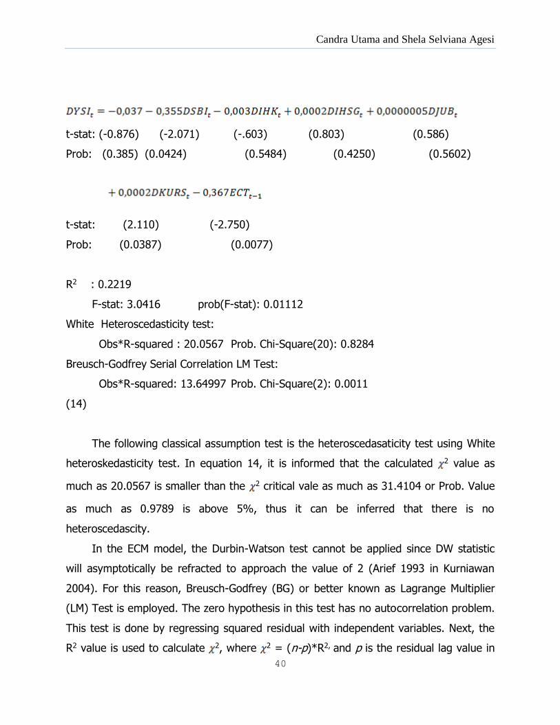
DISCUSSION AND ESTIMATION RESULT
Empirical Model Test
The selection of model is an important measure in empirical modeling. Faults in
determining the correct function form lead to problems in specification and inconsistent
estimation parameters. In this case, this study employs the criteria test of Akaike
Information criteria (AIC) and Final Prediction Error (FPE) to select variables that will be
used in the model.
Table 1. AIC and FPE Calculation Result
Step
1 0.154508 0.154511
Candra Utama and Shela Selviana Agesi
40
2 0.152949 0.152957
3 0.125076 0.125090
4 0.118707 0.118734
5 0.105126 0.105167
6 0.092893 0.092950
Source : Authors’ Calculations
The result of model test is then compared from every step conducted. If the AIC
and FPE values of each step are smaller than the values from the the previous step, the
variables then can be used in the model. As presented in table 1, step 2 of the AIC and
FIP are smaller than those of step 1, then step 4 is smaller than step 3, while step 6 is
smaller than 5. Therefore, all the variables that will be used are proper in this study.
Unit Root Test
Unit root test to all variables used is necessary to meet the validity of ECM analysis. The
data is called stationary if they can fulfill these three elements, i.e. possessing a
constant average, a constant variance, and a constant covariance in every time unit
(Thomas, 1997). Table 2 presents the result of the unit root test using the Augmented
Dickey Fuller test at level phase. As presented in table 2, there is only one stationary
variable at the level phase, i.e. YSI variable (at the significance level of 5%) while SBI,
IHK, IHSG, JUB, and KURS are non stationary.
Table 2. Unit Root Test at the Level Phase
Variable ADF Value Probability Description
YSI -3.359419 0.0158 Stationary
SBI -1.745498 0.4043 Non Stationary
IHK -2.823976 0.0601 Non Stationary
IHSG -0.584149 0.8668 Non Stationary
JUB 2.272225 0.9999 Non Stationary
KURS -1.639015 0.4574 Non Stationary
Source : Authors’ Calculations
The Effect of Macroeconomic Variables On The Yield Spread on Indonesian Government’s
Bond
165
As only one variable that stationary, we need to conduct the Augmented Dickey
Fuller phase at first-difference phase. As presented in table 3, at first difference, all the
variables used in this study are integrated (stationary) with a probability value of below
5%. The stationary condition at a similar degree is one of the requirements to see the
potential relationship and to avoid a spurious regression.
Table 3. Unit Root Test at the First Difference Phase
Variable ADF Value Probabilitty Description
Yield Spread -6.933019 0.0000 Stationary
Interest Rate -3.313056 0.0180 Stationary
IHK -6.058594 0.0000 Stationary
IHSG -4.123914 0.0017 Stationary
JUB -10.23920 0.0001 Stationary
Exchange Rate -3.170666 0.0261 Stationary
Source : Authors’ Calculations
Cointegration Test
Following the unit root test, the next step is conducting the cointegration test to
see the presence of long term relationship amongst variables. Johansen test of
cointegration test result is presented in table 4, showing that the Unrestricted
Cointegration Rank Test (Trace) at α=5% shows at least 4 cointegration equation. As
for the test using Unrestricted Cointegration Rank Test (Maximum Eigenvalue), it
demonstrates that there are at least 2 cointegration variables.
Table 4. Cointegration Test Using Johansen Contegration Test
Unrestricted Cointegration Rank Test (Trace)
Hypothesized Trace 0.05 No. of CE(s) Eigenvalue Statistic Critical Value Prob.**
None * 0.469853 136.6852 95.75366 0.0000
At most 1 * 0.453874 92.89766 69.81889 0.0003
At most 2 * 0.257189 51.15920 47.85613 0.0237 At most 3 * 0.212377 30.64454 29.79707 0.0399
Candra Utama and Shela Selviana Agesi
40
At most 4 0.174664 14.17174 15.49471 0.0783
At most 5 0.013333 0.926169 3.841466 0.3359 Trace test indicates 4 cointegrating eqn(s) at the 0.05 level
* denotes rejection of the hypothesis at the 0.05 level **MacKinnon-Haug-Michelis (1999) p-values
Unrestricted Cointegration Rank Test (Maximum Eigenvalue) Hypothesized Max-Eigen 0.05 No. of CE(s) Eigenvalue Statistic Critical Value Prob.**
None * 0.469853 43.78752 40.07757 0.0183
At most 1 * 0.453874 41.73846 33.87687 0.0047
At most 2 0.257189 20.51466 27.58434 0.3066 At most 3 0.212377 16.47280 21.13162 0.1984 At most 4 0.174664 13.24557 14.26460 0.0720
At most 5 0.013333 0.926169 3.841466 0.3359 Max-eigenvalue test indicates 2 cointegrating eqn(s) at the 0.05 level * denotes rejection of the hypothesis at the 0.05 level
**MacKinnon-Haug-Michelis (1999) p-values
Source : Authors’ Calculations
Estimation Result of the Long Run Model
In equation (12) as follows, it can be seen the estimation result of long run
model. Then, the residual of this model will be used as ECT variable in ECM model.