DI

SC

US

SI

ON

P

AP

ER

S

ER

IE

S

Forschungsinstitut zur Zukunft der ArbeitInstitute for the Study of Labor

The Effect of Migration on Income Growth and Convergence: Meta-Analytic Evidence

IZA DP No. 4522

October 2009

Ceren OzgenPeter NijkampJacques Poot

The Effect of Migration on

Income Growth and Convergence: Meta-Analytic Evidence

Ceren Ozgen VU University Amsterdam

Peter Nijkamp

VU University Amsterdam

Jacques Poot University of Waikato

and IZA

Discussion Paper No. 4522 October 2009

IZA

P.O. Box 7240 53072 Bonn

Germany

Phone: +49-228-3894-0 Fax: +49-228-3894-180

E-mail: iza@iza.org

Any opinions expressed here are those of the author(s) and not those of IZA. Research published in this series may include views on policy, but the institute itself takes no institutional policy positions. The Institute for the Study of Labor (IZA) in Bonn is a local and virtual international research center and a place of communication between science, politics and business. IZA is an independent nonprofit organization supported by Deutsche Post Foundation. The center is associated with the University of Bonn and offers a stimulating research environment through its international network, workshops and conferences, data service, project support, research visits and doctoral program. IZA engages in (i) original and internationally competitive research in all fields of labor economics, (ii) development of policy concepts, and (iii) dissemination of research results and concepts to the interested public. IZA Discussion Papers often represent preliminary work and are circulated to encourage discussion. Citation of such a paper should account for its provisional character. A revised version may be available directly from the author.

IZA Discussion Paper No. 4522 October 2009

ABSTRACT

The Effect of Migration on Income Growth and Convergence: Meta-Analytic Evidence*

We compare a set of econometric studies that measure the effect of net internal migration in neoclassical models of long-run real income convergence and derive 67 comparable effect sizes. The precision-weighted estimate of beta convergence is about 2.7%. An increase in the net migration rate of a region by one percentage point in increases the per capita income growth rate in that region on average by about 0.1 percentage points, thus suggesting an impact of net migration that is more consistent with endogenous self-reinforcing growth than with neoclassical convergence. Introducing a net migration variable in a growth regression increases the estimate of beta convergence slightly. Studies that use panel models or IV estimation methods yield smaller coefficients of net migration in growth regressions, while the opposite holds for regressions controlling for high-skilled migration. JEL Classification: O15, O18, R23, R11 Keywords: internal migration, economic growth, convergence, meta-analysis,

neoclassical model, regional disparities Corresponding author: Jacques Poot Population Studies Centre University of Waikato Private Bag 3105 Hamilton 3240 New Zealand E-mail: jpoot@waikato.ac.nz

* Earlier versions of this paper were presented at the 55th Annual North American Meetings of the Regional Science Association International (RSAI), 20-22 November 2008, Brooklyn, New York; the Workshop on Creative, Intellectual and Entrepreneurial Resources for Regional Development, 15-16 June 2009, Tinbergen Institute & VU University, Amsterdam; the Workshop on Determinants and Effects of Interregional Mobility, 1-3 October 2009, Alghero, Sardinia, Italy; and the 46th Annual Meeting of the Japan Section of RSAI, 10-12 October 2009, Hiroshima, Japan. We thank Bernard Fingleton, Geoffrey Hewings, Mario Larch, Yasuhide Okuyama and three anonymous referees for useful comments. We are grateful to Etsuro Shioji and Sari Pekkala Kerr for providing additional primary study results.

 THE EFFECT OF MIGRATION ON INCOME GROWTH AND CONVERGENCE: 

 META‐ANALYTIC EVIDENCE   1. Introduction  

Migration  is an  important means  through which people can  improve  their economic well‐

being and quality of life. In general, net population movement tends to be oriented towards 

prosperous areas which offer higher real income prospects. Fuelled by migration, the global 

urban  population  grew  12.7  times  in  the  20th  century  (UNFPA,  2007),  while  the  world 

population increased by about a factor of four (UN, 2009).1 The concentration of population 

in  particular  cities  and  regions  often  coincides with  increasing  regional  disparities within 

countries  due  to  agglomeration  effects  (e.g.,  Fujita  and  Thisse,  2002).  This  prompts  the 

question  how  those  that  leave  a  region,  and  thereby  become  a  newcomer  in  a migrant 

receiving  region, affect  the spatial distribution of  income. The  redistribution of population 

across cities and regions  invokes a wide range of short‐run and  long‐run supply effects and 

demand  effects  of  which  the  joint  impact  is  ultimately  an  empirical  matter.  Our  study 

focuses  therefore  on  the  consequences  of  net  internal migration  for  spatial  disparities  in 

economic growth, and for the speed of income convergence. 

 

Many researchers emphasize the labour‐supply effect of migration in a standard neoclassical 

framework.  Migration  is  in  this  framework  a  mechanism  for  reducing  spatial  income 

differentials (e.g., McCann, 2001). Yet many others oppose the standard growth model, and 

point,  for  example,  to  the  importance  of migrants’  characteristics  such  as  youthfulness, 

entrepreneurship and skills that, together with their impact on aggregate demand, may have 

growth‐enhancing  effects,  particularly  in  an  agglomerated  economy  (e.g.,  Poot,  2008). 

Simply  in terms of aggregate demand and scale of the economy, regions  losing population 

through  migration  may  face  economic  contraction,  whereas  regions  gaining  population 

through migration may  benefit  from  an  expansionary  effect  on  output,  employment  and 

income.  However,  studies  on  the  consequences  of migration  show  that  the  transfer  of 

human capital from one place to another is a critical aspect (see Kanbur and Rapoport, 2005; 

1 The global urban population grew  in this period from 220 million to 2.8 billion, while the world population grew from 1.7 billion to about 6.8 billion.

1

Rappaport, 2005). In particular, skill‐selective mobility may have profound impacts on origin 

and destination places, a finding that may be at odds with a neoclassical framework.  

 

Since the 1990s, the economic growth literature has produced a number of studies that have 

analysed  the  role  of  internal migration  on  per  capita  income  convergence.  The  evidence 

produced by the current  literature regarding the effects of migration  is not yet conclusive. 

The observed results may depend on various study characteristics, research methodologies, 

type  of  data,  and  the  spatial  scale  of  measurement  at  which  the  research  has  been 

conducted (Nijkamp, 2009). Additional  insight  into the quantitative effect of migration may 

be obtained by analysing the variation in the estimated effect sizes across a range of primary 

studies. Meta‐analytical techniques provide appropriate tools for this research task. The aim 

of the present study  is therefore to analyse the effect of migration on  income convergence 

by  means  of  a  meta‐analytic  evaluation  of  various  econometric  studies  that  have 

incorporated  migration  as  an  explanatory  variable  in  regression  models  of  income 

convergence. 

 

In Section 2 we present a brief and selective  review of empirical studies on  the  impact of 

migration  on  economic  growth.  Section  3  describes  a  short  explanation  of  our  meta‐

analytical technique.  The data obtained from a purposive selection of past empirical studies 

is given  in Section 4. We present  the  results of our meta‐regression analysis  in Section 5. 

Section 6 offers concluding remarks. 

 

2. Impact of Migration on Income Convergence: A Review 

Can  internal migration contribute to the absorption of external economic shocks  in regions 

and  to  the  alleviation of  regional  inequalities? An  extension of  the  Solow‐Swan model of 

growth  in a composite good economy that  incorporates migration of homogeneous  labour 

highlights  that as  long as  there are diminishing  returns  to  labour, workers move  from  low 

income to high  income regions and migrants have on average  low  levels of human capital, 

migration accelerates income convergence (e.g., Barro and Sala‐i‐Martin, 2004). When there 

are  no  barriers  to  factor  mobility,  labour  and  capital  move  in  this  model  in  opposite 

directions and both contribute to a reduction in spatial disparities in capital per effective unit 

of labour, as well as income per capita. Migration in the form of a movement of labour from 

2

poor to rich areas lowers capital intensity (increases the return to capital) in the destination 

region, and  increases capital  intensity  (lowers the return to capital)  in the region of origin. 

Thus, when  the  same  technologies  are  used  everywhere, migration  speeds  up  per  capita 

interregional convergence in capital intensity and income (Polese, 1981).  

 

Barro  and  Sala‐i‐Martin  (2004) provide  a detailed  explanation of  this phenomenon  in  the 

context of  the neoclassical growth model. They conclude  that  if migration  is an  important 

source  of  convergence,  and  if  the  endogeneity  of  migration  in  growth  regressions  is 

controlled  for,  the  estimated  beta  coefficient  (the  effect  of  initial  income  on  economic 

growth  during  the  transition  to  the  steady‐state  growth  path)  should  become  smaller  in 

regressions  that  include  a migration  variable.  In  addition,  in  a world  in which  the  same 

composite  good  is  produced  everywhere  with  the  same  technology  with  homogeneous 

labour,  increasing  population  growth  through  net  inward  migration  lowers  the  rate  of 

economic growth (growth in income per capita). The coefficient of the migration variable in 

a growth regression, when properly  instrumented  to account  for endogeneity, would  then 

be negative. 

 

Both  labour mobility  and  capital mobility will  bring  the  capital  intensities  of  sending  and 

receiving regions closer, which  is the mechanism through which factor mobility contributes 

to  interregional  income convergence. Clearly,  the  impact of net migration on convergence 

and growth will, in practice, depend on interregional differences in capital intensity, the skill 

levels of the migrants, the extent to which migration  induces gross fixed capital formation, 

the  composition  of  output  and  the  associated  technologies,  and  the  extent  to  which 

migration affects technological change (e.g.,  McCann, 2001; Nijkamp and Poot, 1998).  

 

If out‐migrants possess on average  substantially higher human  capital  than  stayers,  it will 

take longer for sending economies to reach their long‐run steady state. Additionally, the exit 

of  labour  from  poorer  regions may  lower  gross  fixed  capital  formation  in  such  regions. 

Therefore,  the disincentive effect of outmigration on  investment may dominate  the direct 

effect  of  outmigration  on  labour  supply  and wages,  so  that  outward migration may  slow 

down  wage  growth  rather  than  increase  it  as  the  neoclassical  model  would  predict 

(Rappaport, 2005). If net migration increases real per capita income growth, then the speed 

3

at  which  the  region  reaches  its  steady‐state  growth  path  increases.  Consequently,  the 

presence  of  a  significantly  positive  net  migration  variable  in  the  growth  regression  is 

expected  to  increase  the estimate of beta convergence. However,  the  impact of migration 

on growth and the speed of convergence is ultimately an empirical matter. 

 The following econometric specification  is commonly used  in the  literature to measure the 

impact of migration on economic growth and convergence:  

(1/T) . log(yi,t/yi,t‐T) = α ‐ [(1 ‐ e‐βT)/T]. [log(y i,t‐T)] + γ mi,t + other variables + error term,       (1)

                 

where the dependent variable is the average annual growth rate of per capita income; yi,t is 

the per capita income in region i in year t; T is the time span of the data; β is the annual rate 

at which an economy converges to its own long‐run steady state, and γ is the coefficient of 

the annual net migration rate mi,t. This rate is calculated as the average annual net migration 

flow (in‐migration into region i minus out‐migration from region i) between the years t‐T and 

t divided by the total population at the beginning of the observation period. Mathematically, 

mi,t = [(NMi,t‐T,t/T)/Pi,t‐T]. Virtually all studies of beta income convergence (so‐named, because 

these  studies  aim  to  estimate  β  in  equation  (1))  adopt  specification  (1)  or  its  linearized 

equivalent, but many studies among these  implicitly assume that γ = 0. The present meta‐

analysis  focuses  on  evidence  that  explicitly  tests  that  γ  ≠  0.  The  coefficient  of  interest  is 

therefore γ, the coefficient of the net migration variable. In the neoclassical model we would 

expect that γ < 0 once we can treat migration as exogenous with respect to the error term. 

We also expect that regressions that  impose that γ = 0, while  in  fact γ < 0, show a greater 

effect of initial income on growth, i.e. a greater β (Barro and Sala‐i‐Martin, 2004, p.492). The 

bias in the estimation of β due to the omitted net migration variable is then positive. We will 

use βo to refer to an estimate of β when net migration rate variable is omitted, and βi to 

refer  to an estimate of β when  the net migration variable  is  included. When  the net 

migration rate variable  is estimated to be negative  (the neoclassical case), then we expect 

βo‐βi > 0; but when the estimated coefficient of net migration is positive, then we expect βo‐

βi < 0. The data described in Section 4.2 confirm this intuition.  

 

4

Various  studies on  the effect of  internal migration  in  the neoclassical growth model have 

yielded  diverse  results.  Barro  and  Sala‐i Martin  (2004,  Table  11.7)  find  that  the  effect  of 

internal migration  on  growth  in  per  capita  income  across  regions  in  the  US,  Japan  and 

various European countries  is statistically  insignificant once  instrumental variables account 

for  endogeneity  of  net migration.  The  effect  on  the  estimated β  is  inconclusive  as well.2 

Similarly, Cardenas  and Ponton  (1995)  report  a  negligible  impact  of migration  on  income 

convergence  in  Colombia  (1960‐1989),  and  Gezici  and  Hewings  (2004)  find  no  effect  of 

migration  on  reducing  regional  disparities  in  Turkey  (1987‐1997).  In  contrast,  Kırdar  and 

Saraçoğlu  (2008)  detect  a  negative  impact  of migration  on  regional  growth  rates  and  a 

decrease  in  the  estimate  of  beta  convergence  in  Turkey  (1975‐2000).  Such  apparently 

contradictory results, even for the same country, warrant a systematic investigation into the 

causes of such differences in conclusions. 

 

A  substantial  literature has emerged  to  consider  the  very  slow  convergence,  convergence 

only within clusters or “clubs”, or divergence observed in reality (see, e.g., Islam 2003 for a 

review  of  the  literature).  The  removal  of  regional  disparities  through migration  and  local 

labour market adjustment take such a  long time that relying exclusively on this adjustment 

mechanism may  lead  to underutilization of  resources  in depressed  regions  (Pissarides and 

McMaster, 1990). Both migratory behaviour and migrant characteristics have an  important 

influence on the convergence process (Greenwood, 1975). There are two major  impacts of 

labour migration: the scale (size) effect, and the composition effect. A high level of outward 

migration of skilled  labour may hurt scale and productivity of  the  labour‐exporting  region, 

and benefit the labour‐importing region. Furthermore, such migration can be persistent, and 

may not die away over time. For example, Williamson (1991) observed that,  in the US, the 

real  wage  gap  between  urban  and  rural  areas  showed  a  striking  persistence  over  five 

decades  in 1890‐1941, despite a continuous unidirectional migration  flow  into urban areas 

(Reichlin  and  Rustichini,  1998).  Evidence  from many  countries  suggests  that  ignoring  the 

heterogeneity of labour may bias the estimates of the effect of migration on growth (Shioji, 

2001).  The  impact  of  migration  on  regional  inequalities  is  unclear  unless  one  explicitly 

considers  the  skills of  the migrants. Migrants with higher human  capital endowments are 

2 In some countries  β increases, in others the estimated parameter decreases.

5

expected to search for job‐opportunities over wider geographical areas and are clearly more 

mobile (McCann, 2001). Migration can play a role as an adjustment mechanism from which 

all  regions  benefit,  but  it  can  also  favour  the  economy  of  only  the  recipient  region. 

Heterogeneous  labour may offset  the  scale effect of migration  through  the  change  in  the 

ratio between skilled and unskilled workers  (Etzo, 2008).  Indeed,  the skills of  the migrants 

determine what happens to the economic opportunities in a source region when a selected 

subsample of its population moves elsewhere (Borjas, 1999). Inflow of skilled labour can lead 

to  an  upward  shift  in  productivity  in  the  recipient  regions.  Although  migration  allows 

workers  to  maximize  their  individual  utility,  it  may  also  increase  regional  disparities  in 

income per capita at  the aggregate  level, depending on  the  skills of migrants  (Fratesi and 

Riggi, 2007).  

 

Despite  the  earlier  noted  persistence  of migration  patterns,  the  volume  and  direction  of 

migration may eventually  change. Certain  factors  such  as  agglomeration externalities  and 

relative wage  dispersion  effects  are  quite  crucial  to  the  impact  of migration  on  receiving 

regions.  Recent  trends  indicate  a  massive  movement  towards  cities.  The  theory  of 

intervening opportunities suggests that opportunities matter more to migrants than distance 

(Stouffer, 1940). Cities are places where  there are  relatively more opportunities. They are 

also the places that bring people together, and the externalities created by the diversity of 

people in cities are the drivers of economic growth (Glaeser et al., 1992). While these effects 

are greatest  in big cities, such cities also simply offer more jobs (Molho, 1986). Greenwood 

and Hunt (1989) confirm that jobs and wages have a considerably higher direct effect on net 

metropolitan migration  of  employed  persons  than  location‐specific  amenities. Of  course, 

while  the  job market  remains an  important determinant of migration patterns,  the spatial 

distribution  of  the  quantity  and  quality  of  jobs  may  not  provide  a  full  explanation  of 

observed migration patterns. Such patterns may also be based on other locational attributes 

(Cushing and Poot, 2004). For example, Gallup et al. (1999) concluded that landlocked areas, 

being  geographically  disadvantaged,  are  economically  disadvantaged.3  This  highlights  that 

economic geography, the attributes of migrants, their responsiveness to spatial disparities, 

regional economic adjustment processes and externalities associated with migration are all 

3 The 28 landlocked countries outside Europe, containing 295 million people in 1995, are among the poorest in the world. 

6

important, but  complex, drivers of empirical estimates of  the  impact of net migration on 

growth and convergence. 

 

In  conclusion,  the  effect  of  migration  on  income  growth  and  convergence  remains  an 

ongoing  research  issue. Past empirical  studies appear  to have  led  to contradictory  results. 

The challenge is to identify the theoretical framework that is most strongly supported by the 

empirical  findings.  This  is where meta‐analysis  can  play  an  important  role. Meta‐analytic 

techniques  provide  a  systematic  analysis  of  the  available  empirical  evidence  from 

independently undertaken  studies. Such  techniques permit us  to  identify  the  relationships 

between the measured effects of migration and relevant study characteristics such as data 

source,  scientific method,  and  the  choice  of  geographical  boundaries. We will  therefore 

utilize  meta‐analysis  in  this  paper  as  a  method  to  compare  the  empirical  findings 

quantitatively  and  to  identify  the  causes  for  observed  differences  in  the  impact  of  net 

migration on economic growth. 

 

3. A Short Introduction to Meta‐analysis: Analysis of Analyses 

During  the  last  half  century  there  has  been  an  explosive  growth  of  empirical  economic 

research.  The  research  findings  on  a  particular  topic  may  indicate  a  great  variety  of 

conclusions and can be confusing and conflicting about central  issues addressed by theory 

and practice. Narrative literature reviews in economics may not allow the researcher to distil 

credible and accurate generalizations from primary studies (Rosenthal and DiMatteo, 2001). 

Instead,  meta‐analysis  can  offer  a  clearer  idea  of  the  variation  in  findings  across  the 

literature  and  provides  systematic  details  of  the  studies  through  coding  their  varying 

characteristics, as well as the basis on which the research has been conducted  (Lipsey and 

Wilson, 2001). Meta‐analysis has clarified a controversial area of  research  in various cases 

(Stanley, 2001). By means of meta‐analysis it is possible to combine the numerical outcomes 

from  various  studies,  to  gauge  the  accuracy  of  relationships,  and  to  explain  the 

inconsistencies between research findings.  

 

In  general,  study  characteristics  appear  to matter  for  the  quality  of  the meta‐analytical 

results. Factual or methodological heterogeneity across studies, heteroscedasticity of effect 

sizes (which are the parameter estimates or statistical quantities of interest), and correlation 

7

of  effect  sizes  between  and  within  studies,  can  cause  methodological  problems  when 

interpreting a meta‐analysis.4 Heterogeneity, defined as a variation of the mean among the 

effect sizes that are collected from primary studies, is a major concern in many comparative 

analyses. When the distribution of effect sizes is heterogeneous, then the analysts must look 

for  the  reason  for  the disagreement on  the magnitude of  the  effects  among  the  studies. 

Moreover,  “the more  unexplained  variance  across  studies, …  ,  the more  uncertain  is  the 

meaning  of  the  summary  statistics”  (Lipsey  and  Wilson,  2001).  While  allowing  for 

unexplained  factors  that  drive  some  of  the  variation  in  effect  sizes,  the mean  effect  size 

should be clear and interpretable.  

 

Therefore, heterogeneity  in meta‐analytical studies  is handled  in two main ways: firstly, by 

focusing on  explaining  the  variation;  and  secondly, by  analysing  the mean  effect  sizes by 

making  particular  assumptions  regarding  their  distribution.  The  most  commonly  used 

method  for  the  first  approach  is meta‐regression  analysis which  explains  the  variation  of 

effect  sizes  in  terms  of  regressors  that  represent  various  study  characteristics.5  For  the 

second approach, random and fixed effect models are used to predict population effect sizes 

on  the basis of  the sample of effect sizes collected  from primary studies  (e.g., Nelson and 

Kennedy,  2008).  The  random  effects  model  assumes  that  the  underlying  population 

parameter  is  itself  drawn  from  a  distribution. Hence,  there  are  two  sources  of  variation: 

within and between‐study variance.6 While the random effects model provides a systematic 

methodology  to  manage  between‐  and  within‐study  variation,  the  fixed  effect  model 

assumes no heterogeneity. Samples of effect sizes can of course be split  into sub‐samples 

that on a priori or statistical grounds may be assumed to be homogeneous. 

 

In  the  fixed  effect model,  primary  studies  estimate  a  fixed  population  effect.  For  a  fixed 

effect model,  let  Ti  be  the  observed  effect  size  of  study  i,  i=1,….,k  .  It  is  assumed  that 

4  For  a  recent  discussion  on  ‘best  practice’  in  meta‐analysis  in  economics  (with  particular  reference  to environmental economics), see Nelson and Kennedy (2008). 5 Such descriptors are commonly study attributes that can be represented by categorical variables, which are then represented  in a meta‐regression analysis by binary dummy variables. Not all attributes are qualitative: the sample size of a primary study can be an important integer variable. 6 The  common use of  this  approach  refers  to  the  cases where  the  source of  variation  cannot be  identified (Sutton et al., 2000).  

8

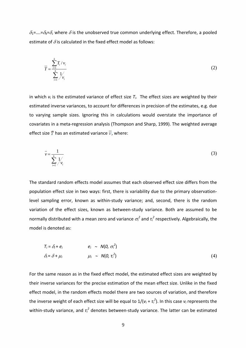
δ1=….=δk=δ, where δ is the unobserved true common underlying effect. Therefore, a pooled 

estimate of δ is calculated in the fixed effect model as follows: 

 

1

1

/

1

k

i ii

k

ii

T vT

v

=

=

=∑

∑ (2) 

 

in which vi is the estimated variance of effect size Ti.  The effect sizes are weighted by their 

estimated inverse variances, to account for differences in precision of the estimates, e.g. due 

to  varying  sample  sizes.  Ignoring  this  in  calculations would  overstate  the  importance  of 

covariates in a meta‐regression analysis (Thompson and Sharp, 1999). The weighted average 

effect size   has an estimated variance  , where:  

 

1

1

1k

ii

v

v=

=

∑ (3)

 

The standard random effects model assumes that each observed effect size differs from the 

population effect size in two ways: first, there is variability due to the primary observation‐

level  sampling  error,  known  as within‐study  variance;  and,  second,  there  is  the  random 

variation  of  the  effect  sizes,  known  as  between‐study  variance.  Both  are  assumed  to  be 

normally distributed with a mean zero and variance σi2 and τi

2 respectively. Algebraically, the 

model is denoted as: 

 

Ti = δi + ei    ei   ∼   N(0, σi2)                    

δi = δ + µi   µi   ∼   N(0, τi2)  (4) 

 

For the same reason as in the fixed effect model, the estimated effect sizes are weighted by 

their inverse variances for the precise estimation of the mean effect size. Unlike in the fixed 

effect model, in the random effects model there are two sources of variation, and therefore 

the inverse weight of each effect size will be equal to 1/(vi + τi2). In this case vi represents the 

within‐study variance, and τi2 denotes between‐study variance. The  latter can be estimated 

9

by considering the distribution (specifically the variance) of the observed sample of Ti (e.g., 

Shadish and Haddock, 1994, p. 274). 

 

The  fixed  and  random  effects weighted mean  effect  sizes may  differ  substantially  if  the 

studies are markedly heterogeneous (Egger et al., 1997b). Since the effect sizes are collected 

from various studies, a homogeneity  test  is usually  run  to check whether “the studies can 

reasonably be described as sharing a common effect size” (Hedges and Olkin, 1985).  In the 

literature by far the most commonly used homogeneity statistic  is the Q‐statistic (Engels et 

al.,  2000).7  The  Q‐statistic,  however,  informs  us  only  about  the  presence  or  absence  of 

heterogeneity, and  it does not describe the degree of heterogeneity.8 A generic calculation 

of the Q‐statistic is:  

 

( ) ( )2

.1

/k

i ii

Q T T v=

⎡ ⎤= −⎢ ⎥⎣ ⎦∑   (5) 

 

“If  [the] Q‐value  is higher  than  the upper‐tail critical value of chi‐square at k‐1 degrees of 

freedom,  the observed variance  in  study effect  sizes  is  significantly greater  than what we 

would expect by chance  if all studies share a common population effect size” (Shadish and 

Haddock, 1994).  In meta‐analyses  in economics, this hypothesis  is often rejected. We shall 

see  in  Section  5  that  this  is  also  the  case  in  effect  sizes  that measure  the  impact  of  net 

migration on per capita  income growth.  In the presence of heterogeneity, meta‐regression 

analysis is one way to account for heterogeneity systematically. This method will be applied 

in Section 5. 

 

4. Primary Studies  4.1. Selection of Primary Studies and Study Characteristics 

7 This test is devised by Cochran (1954) and based on a chi square statistic that is distributed with k‐1 degrees of freedom, where k stands for the number of effect sizes (Shadish and Haddock, 1994). 8    “Not  rejecting  the homogeneity hypothesis usually  leads  the meta‐analyst  to adopt a  fixed‐effects model because  it  is assumed  that  the estimated effect sizes only differ by sampling error.  In contrast, rejecting  the homogeneity assumption can lead to applying a random‐effects model that includes both within‐ and between‐studies  variability.  A  shortcoming  of  the Q  statistic  is  that  it  has  poor  power  to  detect  true  heterogeneity among  studies when  the meta‐analysis  includes  a  small  number  of  studies  and  excessive  power  to  detect negligible variability with a high number of studies” (Huedo‐Medina et al., 2006). 

10

The  primary  studies  in  our  meta‐analysis  all  adopt  the  standard  framework  of  the 

neoclassical model  of  growth  and  convergence, while most  discussions  on  the  effect  of 

migration  on  income  convergence  follow  the  path‐breaking  research  by  Barro  and  Sala‐i 

Martin  (1992, 2004).9  In  this paper we will  therefore  address  the  impact of migration on 

income convergence as an empirical research issue. Equation (1) (or a linearization thereof) 

represents the regression equation that all the primary studies used in their analysis. There 

are two parameters of  interest, β and γ,  in equation (1). First we will focus on the effect of 

net migration on growth in per capita income, i.e. the extent of variation in the estimates of 

γ across and within studies. We also check how accounting for the net migration rate affects 

the speed of convergence, β. Jointly, this informs on whether the results of Barro and Sala‐i‐

Martin (2004) are confirmed by other researchers.10

 

The  search  for  papers  was  conducted  systematically  through  software  called  Harzing’s 

Publish or Perish (linked to Google scholar), and alternative search engines such as EconLit. 

Besides references, Harzing’s Publish or Perish also reports the number of citations of each 

document  that  provide  some  measure  of  its  impact. We  used  the  following  keywords: 

migration  and  convergence,  labour mobility,  internal migration,  income  convergence.  The 

literature  search  checked  extensively  electronic  resources  of  published  articles  and 

unpublished  studies,  as  well  as  websites  of  migration‐related  research  institutes,  and 

international organizations. More than 1200 articles were scanned.  

 

However,  many  of  these  do  not  provide  direct  evidence  of  the  impact  of  net  internal 

migration  on  growth  and  convergence.  One  fundamental  problem  is  the  lack  or  limited 

reliability of internal migration data. Growth studies require long‐term time series. Historical 

internal migration data are hard to obtain in many countries. Additionally, the time period of 

the data on migration flows often does not exactly match that of per capita income growth 

data. This makes it hard in empirical research to calculate the effect of migration for various 

periods,  therefore,  convergence  studies  tend  to  report  relatively  few  regressions  that 

9 The foundation for all primary studies are the neoclassical closed economy models of Ramsey (1928), Solow (1956), Cass (1965) and Koopmans (1965). All predict that the per capita growth rate over a given period tends to be  inversely related to the  level of output or  income per capita at the beginning of the period  (Barro and Sala‐i Martin, 1992).  10 Barro and Sala‐i‐Martin estimated equation (1) with data on the US, Japan and some European countries. 

11

include migration variables. Moreover, many of the studies that directly assess the effect of 

migration  on  income  convergence  have  been  fairly  recent, with  60  percent  having  been 

published after 2000.11

 

An additional problem that limits the number of comparable estimates in this study – and in 

economic  research generally –  is  that  innovation and uniqueness of empirical modelling  is 

rewarded  by  referees  and  editors  of  journals,  while  replication  is  not  encouraged 

(Hamermesh, 2007). Meta‐analysis requires the acquisition of a cluster of studies concerned 

with  the  same  research  question  that  use  a  common  econometric  specification,  i.e.  a 

common metric of measurement. This significantly reduces the pool of empirical estimates 

that  can be potentially  suitable  for  summarising by meta‐analysis.  In  the present  context, 

while the literature on convergence is huge, only papers that use, or build on, the migration‐

extended  convergence  model  suggested  by  Barro  and  Sala‐i  Martin  (1992,  2004)  were 

selected. The selected studies for meta‐analysis were all published after 1991.  

 

The paper selection process initially yielded 17 studies with 94 observations. However, some 

serious comparability problems remained, and five papers had to be dropped. From the 12 

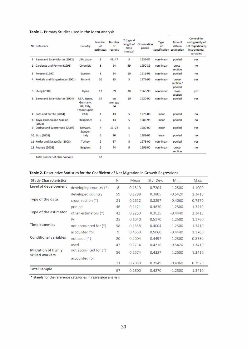
remaining papers, 67 estimates of β and γ  were obtained. Table 1 describes the sources of 

the estimates and some key features of these studies.12  

 

Table 1 about here 

 

A  larger  number  of  studies  would  have  generated  a  larger  set  of  observations  on  the 

statistical significance of the impact of net migration on growth, but in the present study the 

focus is on deriving estimates of the magnitude of the effect, which requires the regression 

models to be directly comparable  (with at most corrections  for differences  in terms of the 

scale of variables or  the effect of  linearization). The  trade‐off  is  that greater comparability 

(and consequently greater homogeneity of  the  included estimates) reduces  the size of  the 

11 Even excluding Barro and Sala‐i‐Martin (2004), whose estimates were originally published in 1995. 12 Several papers used the same analytical framework but did not generate estimates that corresponded with equation (1) or its linearized equivalent, applied to the impact of net internal migration on interregional growth differentials. Examples are Gezici and Hewings (2004), Maza (2006) and Cashin and Loayza (1995). 

12

sample  of  estimates. However,  it  should  be  noted  that  the  67  available  estimates  cover 

nonetheless a diverse range of countries from different parts of the world. 

 

The transformations that have been applied to some study findings concern the coefficients 

of  initial  income and of net migration. Firstly, to ensure comparability of the net migration 

coefficients, such coefficients were converted, if necessary, to the equivalent coefficient for 

a  variable  that measures  the  ratio  of  annual  net migration  over  total  initial  population. 

Secondly,  if  the  coefficient  of  the  initial  income  variable  was  given  by  linear  regression 

estimation  in  a  primary  study,  then  the  estimated  coefficient  was  turned  into  its  non‐

linearized equivalent according to b =  ‐[(1  ‐ e‐βT)/T] and, hence, β =  ‐ln(1+bT)/T.  In most of 

the papers,  the dependent variable  in  the  regressions was growth  in personal  income per 

capita, but in some cases (Chile, Norway, Sweden, Italy) the dependent variable referred to 

growth in Gross Regional Product per capita. This had no impact on the meta‐analysis. 

 

4.2. Descriptive Statistics 

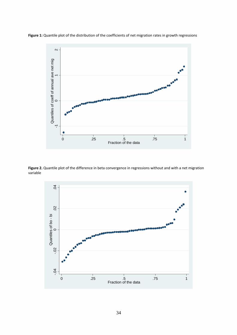
Using  the  67  effect  sizes  obtained  from  the  studies  listed  in  Table  1,  the  distribution  of 

estimates of  γ  (coefficient of net migration) are within a  range of  ‐1.25  to 1.34,  clustered 

around  zero. The mean value  is 0.18, with a  standard deviation of 0.43.13 Even without a 

formal test, this large standard deviation is indicative of considerable heterogeneity. Figure 1 

shows the quantile plot of the estimated coefficients. Both the mean value and the median 

value  (0.13) suggest a small positive  impact of migration on  the per capita  income growth 

rate. However,  the magnitude of  the effect can only be meaningfully estimated when  the 

precision  of  the  estimates  is  taken  into  account  by means  of  the  fixed  effect  or  random 

effects  estimator,  as will be discussed below. Here we  simply note  that only  2  of  the  67 

coefficients of net migration had a  statistically  significant negative value  (at  the 5 percent 

level), while 27 of the 67 estimates had a statistically significant positive value. 

 

Figure 1 about here 

 

13 All estimations have been carried out in Stata 10.1. The meta-analysis estimation software is outlined in Sterne (2009).

13

The Q‐statistic of heterogeneity of effect sizes shown in Figure 1 is 336.3, with 66 degrees of 

freedom. Hence, the null hypothesis of homogeneity is conclusively rejected with a p‐value< 

0.001.  I2  (a measure of variation  in  the estimated gamma attributable  to heterogeneity)  is 

80.4 percent. The  fundamental question  is the extent to which the variation  in effect sizes 

across studies is systematic rather than due to random variation. Explaining this variation is 

not only the main interest in the present study, but may also provide additional insight into 

discussions  in  the  recent  literature  on  the  effect  of  net migration  on  growth  and  on  the 

convergence coefficient. We explain this variation by utilizing a set of moderator variables, in 

the  form  of  binary  dummy  variables.  These  present  the  characteristics  of  the  primary 

studies.  

 

The moderator variables, which are  study  features  that may explain heterogeneity among 

the observed net migration coefficients, are presented in Table 2. Since the variables are in 

the  form  of  binary  dummies,  reference  categories must  be  selected  for meta‐regression 

analysis and these are shown by an asterisk (*). The statistical significance of the effect size 

variation, as well as the impact of each study feature on the net migration‐rate coefficient, is 

investigated by means of multivariate analysis  in Section 5. Descriptively, Table 2 suggests 

that  the  coefficient of net migration  is  smaller  in  regressions with pooled data  than with 

cross‐sectional  data, with  Instrumental  Variable  (IV)  estimation, when  time  dummies  are 

accounted for, and when covariates are used. However, the growth impact of net migration 

is  greater when  it  refers  to  highly  skilled workers  only.  The  level  of  development  of  the 

country  does  not  appear  to  have  a  noticeable  influence  on  the  coefficient  of  the  net 

migration rate. 

 

Table 2 about here 

 

The  second  question  of  our  study  is whether  the  speed  of  convergence  is  influenced  by 

including  the  net  migration  variable  in  the  regression  and,  if  so,  to  what  extent?  The 

interquartile range of values of beta convergence in the considered sample of regressions is 

from 0.02 to 0.04 (with 0.02 representing the commonly observed ‘two percent rule’ in the 

14

literature; see Abreu et al. 2005).14 Consistent with  the positive effect of net migration on 

growth noted above,  inclusion of migration  in equation  (1)  increases  the speed of  income 

convergence  slightly:  the average βo  is 0.0302, whereas  the average βi  is 0.0325. Figure 2 

shows  the  distribution  of  the  effect  on  beta  convergence  of  including  a  net  migration 

variable in the regression. The βo‐βi effect varies between ‐0.030 and 0.036, with the average 

being  slightly negative  (‐0.002). This  suggests  that  the migration  variable  in  the economic 

growth  regressions  raises  the beta  convergence  coefficient  slightly,  contrary  to Barro  and 

Sala‐i‐Martin  (2004)  expected.  However,  a  paired  t‐test  indicates  that  the  difference  in 

means  is only  significant at  the 10 percent  level  (one‐sided),  t =  ‐1.59. This  result may be 

compared  with  the  findings  of  Dobson  et  al.  (2006)  who  ran  meta‐regressions  of  beta 

convergence  coefficients  and  found  that  the  inclusion  of  population,  employment  and 

labour  force  growth  (variables  which  may  be  expected  to  have  effects  similar  to  net 

migration rates on beta convergence) in primary studies had mostly an insignificant effect on 

the speed of income convergence.  

 

Figure 2 about here 

 

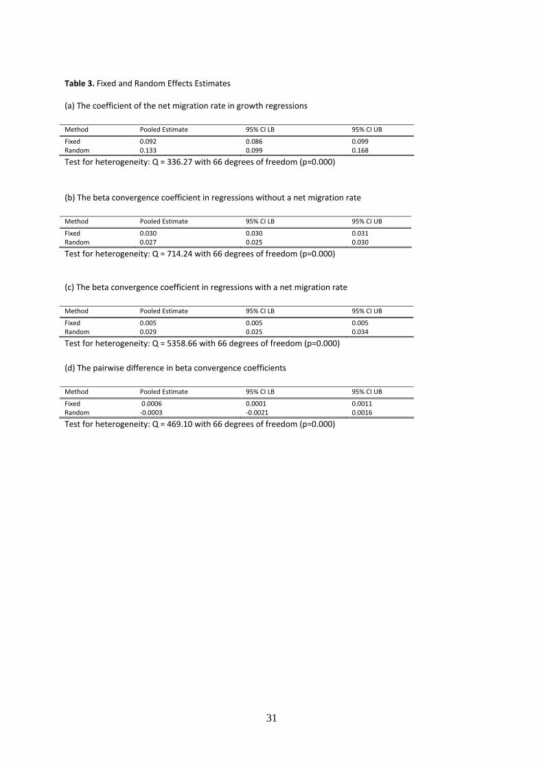
Table 3 reports the fixed and random effects estimates of (a) the coefficient of net migration 

in the growth regressions, (b) the coefficient of beta convergence without net migration, (c) 

the  coefficient  of  beta  convergence  with  net  migration,  and  (d)  the  difference  in  beta 

coefficients. With  weights  determined  by  the  precision  of  the  estimates  of  the  primary 

studies  (as  in equation  (2)),  the  fixed effect estimate of  the coefficient of net migration  is 

0.092. The random effects estimate, which  is always closer to the unweighted mean (0.18, 

see Table 2) is 0.133. Clearly these results suggest that, in rounded terms, an increase in the 

net migration rate by one percentage point  increases the per  income growth rate by about 

0.1 percentage points.  

Table 3.b. also shows that when growth regressions are run without a net migration 

variable  in the specification, the fixed effect estimate of beta convergence  in our sample  is 

0.030. This is larger than the celebrated 2 percent rule, but Dobson et al. (2006) note in their 

meta‐analysis  that  the mean  rate  of  convergence  derived  from  intra‐national  studies  is 

14  Beta  coefficients  of  growth  regressions without  net migration  rate were  not  reported  in  the  published primary study by Shioji (2001). These estimates were kindly provided for the meta‐analysis by the author. 

15

considerably  larger  than  the  rate  obtained  from  cross‐national  studies  and  their  meta‐

sample  average  (unweighted)  of  0.025  for  intra‐national  studies  is  consistent  with  our 

evidence. In our sample of 67 estimates, the fixed effect estimate of beta convergence drops 

considerably  (to  0.005),  when  the  net  migration  variable  is  introduced  in  the  growth 

regression. However,  there  is huge heterogeneity among  these estimates and  the  random 

effects  estimate  is  therefore  more  useful.  The  random  effects  estimate  suggests  that 

introducing a net migration variable into the growth regression increases beta slightly (from 

0.027 to 0.029). 

 

This  small  positive  effect  is  confirmed  by  formally  calculating  a  fixed  and  random  effects 

estimate  of  the  difference.  The  fixed  effects  estimate  is  0.0006  (see  Table  3(d)),  but  the 

random effects estimate has a 95 percent confidence interval running from ‐0.002 to 0.002, 

but with the point estimate being negative, albeit only  in the fourth digit after the decimal 

point  (the precision‐weighted mean  is  ‐0.0003). Given  the considerable heterogeneity,  the 

random effects estimate  is more  informative  in the present context because  it spreads the 

precision weights  (derived  from  the  reciprocals  of  the  squares  of  the  observed  standard 

errors) more evenly than the fixed effect estimate (Borenstein et al, 2009). We conclude that 

including  a  net  migration  variable  in  an  intra‐country  growth  regression  raises  beta 

convergence slightly. 

 

Table 3 about here 

 

Theoretically, if a variable that is correlated with the included variables is excluded from the 

model,  the predicted parameters are biased  (Verbeek, 2004). Therefore, unless  γ = 0,  the 

deletion of net migration rate variable from equation (1) would  lead to biased estimates of 

other parameters, including the estimated beta. If γ = 0, the expected value of βo equals the 

expected value of βi (including an irrelevant variable leaves the estimate unbiased although 

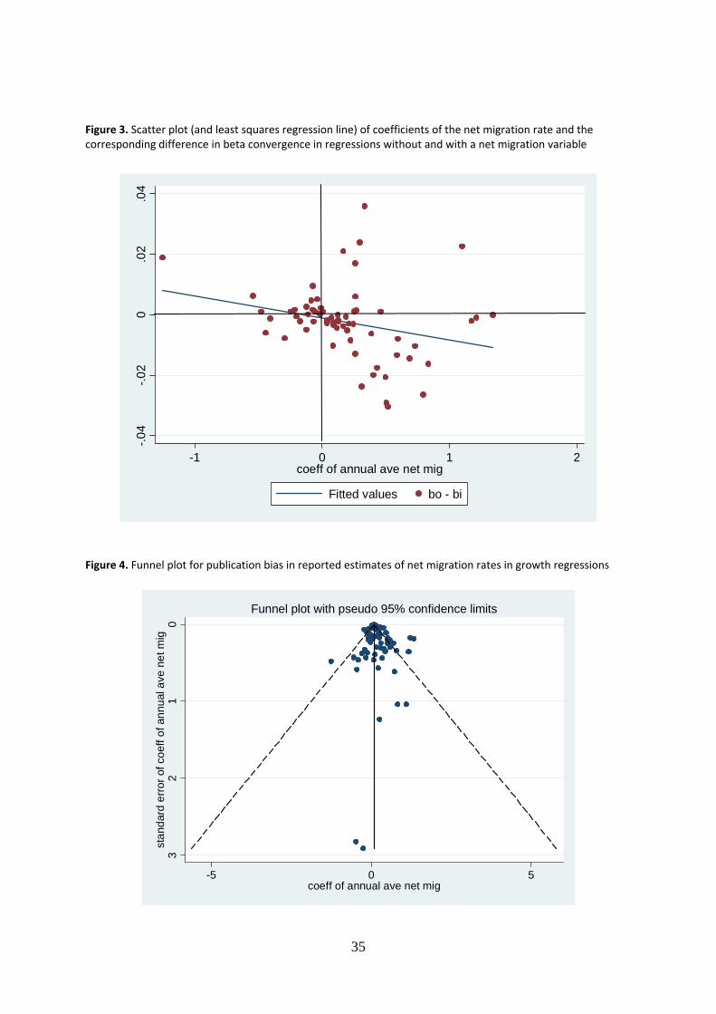
the precision is reduced). Figure 3 presents the bias caused by deletion of the net migration 

rate variable on the difference in estimated beta convergence coefficients without and with 

the  net migration  rate.  The  northwest  quadrant  represents  the  neoclassical  convergence 

combination  of  a  negative  estimate  of  γ,  combined  with  a  positive  bias.  The  southeast 

quadrant  represents  the  endogenous  growth  combination of  a positive  γ  together with  a 

16

negative bias. The precision‐weighted averages of γ and βo−βi are in the southeast quadrant. 

Given  the  heterogeneity,  the  relationship  between  estimated  γ  and  βo−βi  is  not  precise 

(R2=0.07) but statistically significant at the 5 percent level. 

 

Figure 3 about here 

 

4.3. Publication Bias 

 

Publication bias is a highly debated topic in meta‐analysis. The question is whether the effect 

sizes are representative of the population concerned. In general, authors are more likely to 

report  significant  results,  and  what  is  called  the  ‘file‐drawer  problem’  suggests  that 

insignificant results are more likely to be buried in a filing cabinet, although the quality of the 

research may be high. Moreover, publishers are more likely to publish statistically significant 

results than insignificant results (Begg, 1994; Rosenthal and DiMatteo, 2001). Doing a meta‐

analysis by means of a sample which suffers from biased selection of studies and estimates 

may have serious consequences  for the  interpretation of the statistical  inference.  In meta‐

analysis there is also the possibility of an inherent bias due to the selection of only a cluster 

of studies (e.g. using a particular methodology) and the omission of studies not published in 

English.  

 

There  are  various  ways  to  reveal  a  possible  bias.  For  instance,  one  way  to  deal  with 

publication bias is to use a weighting technique that quantifies the methodological strength 

of each study in the analysis (Rosenthal and DiMatteo, 2001). However, such weighting can 

be rather subjective. Here we use a graphical method, the so‐called funnel plot, which plots 

effect sizes against a measure of precision of the estimates. The funnel plot for the estimates 

of  the  coefficient  of  net migration  rates  is  given  in  Figure  4.  Along  the  vertical  axis we 

measure the inverse standard errors of the effect sizes, while the effect sizes themselves are 

measured  along  the  horizontal  axis.  The  broken  lines  represent  the  expected  95% 

confidence intervals for a given standard error, assuming no heterogeneity between studies. 

However, publication bias  is only one of the possibilities that may generate an asymmetric 

funnel plot  (de Dominicis et al., 2008). A  formal statistical test of asymmetry of the  funnel 

plot is known as Egger’s linear regression test (Egger et al., 1997a). The regression equation 

17

may simply be denoted as follows: t*= κ +λs‐1,  in which the t* statistics of the estimates of 

the  primary  regression  coefficient  are  regressed  on  the  corresponding  inverse  standard 

errors, s‐1. The  intercept measures  the asymmetry.  If  the  intercept  is significantly different 

from  zero,  then  this  provides  evidence  for  publication  bias  in  the  dataset  (Sutton  et  al., 

2001).  In our  case,  the observations are distributed  relatively  symmetrically, albeit with a 

positive bias. This is confirmed by Egger’s linear regression test which finds   = 0.517 with an 

associated p‐value of 0.087, i.e. not statistically significant at the 5 percent level.  

 

Figure 4 about here 

 

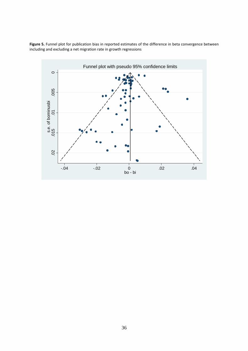
Egger’s  linear  regression  test  provides  some  interesting  results  concerning  the  beta 

coefficients  of  convergence.  In  regressions  without  the  migration  variable,  there  is  no 

evidence of publication bias  in  the estimated beta,   =  ‐0.91 with a p‐value of 0.120. The 

corresponding estimate  in the regressions with the migration variable  is   = 6.13 with a p‐

value of  less than 0.001. Hence, this could be a concern. However, our primary focus  is the 

pair‐wise difference between the two estimated beta, for which we find that   = ‐0.53, with 

a  p‐value  of  0.242. Hence we  conclude  that  the  sample  of  estimates  obtained  from  the 

literature the  impact of net migration rates  in growth regressions has not been affected by 

publication bias.  

 

Figure 5 about here 

 

5.   Meta‐Regression Analysis  

5.1   Methodology 

Meta‐regression analysis is a statistical technique that integrates effect sizes gathered from 

various  independent  studies  and  explains  the  variation  in  them.  This  variation may  come 

from two different sources:   as a result of sampling error (that may vary across studies) or 

due to variability  in the population of effects: namely, unique differences  in the set of true 

population  effect  sizes  (Lipsey  and Wilson,  2001).  The  former  variation  causes  inherent 

heteroscedasticity in the meta‐analysis sample, while the latter causes randomness of effect 

sizes. Moreover, using standard OLS estimation to explain the heterogeneity would  lead to 

18

inefficient  results,  since effect  sizes with a higher  variance would get  the  same weight as 

effect sizes with a lower variance (Koetse et al., 2007). 

 

Meta‐analytical techniques have been developed to address these  issues. The  fixed effects 

regression model assumes that the variation among the effect sizes is fully predictable by a 

number  of moderator  variables  gathered  from  the  primary  studies.  In  general,  the  fixed 

effects  estimator  is  also  known  as  the  ‘inverse  variance‐weighted’ method, whereby  the 

regression weights  are  inversely  proportional  to  the  precision  of  the  estimates,  and  the 

estimation  is conducted by weighted  least squares (WLS). A  linear fixed effects model  is as 

follows: 

 

Ti = β0 + β1xi1 +……….+ βpxip + εi                     εi ∼  N(0, σi2),  (6) 

 

where Ti refers to the estimated effect size i, p denotes the number of moderator variables 

xip; and the βs are the coefficients to be estimated.  In the fixed effects model, the weights 

are equal  to  the  reciprocal of  the  sampling  variances  (weight  for  Ti  is 1/vi),  calculated by 

means  of  the  usually  reported  standard  errors  or  t‐statistics  of  regression  coefficients 

(Hedges, 1994).15  In  standard  statistical packages,  the  coefficients  are  correctly estimated 

with WLS, but  the  standard errors are  calculated by means of a  slightly different  formula 

than in the fixed effect model, hence an adjustment is required.16  

 

In general, the mixed effects model  is considered as a combination of the meta‐regression 

model and the random effects model (Sutton et al., 2000). The mixed effects model allows 

for two variance components by assuming that the effects of between‐study variables such 

as the type of data a study uses, are systematic (subject to sampling error), but that there is 

an  additional  component  that  remains  unmeasured  (and  is  possibly  unmeasurable).  The 

latter represents a random effect in the effect size distribution (Lipsey and Wilson, 2001): 

15 The fixed effect estimates of Table 3 can be obtained by running a WLS regression of the effect sizes on a constant term only. 16 The corrected standard error is generally obtained by dividing the reported standard error by the root mean squared  error  (RMSE)  of  the WLS  regression. However,  using  so‐called  aweights  in  Stata  (which  interprets weights as replications) requires  the reported RSME  to be multiplied by √(N/n)  in which N  is  the sum of  the weights and n is the number of effect sizes. Because Stata reports N in any case, the standard error of the fixed effect estimate can in fact with this software simply be obtained by calculating 1/√N.

19

 

Ti = β0 + β1xi1 +……….+ βpxip + εi + µi               εi ∼  N(0, σi2),   µi ∼  N(0, τi2).   (7) 

 

As  indicated  in Equation  (7),  there are  two error components  referring  to  the within‐ and 

between‐study  variances,  respectively.  These  are  additively  included  in  the  equation  and 

hold  for  the  weights  in  random  variances.  As  a  result  of  including  a  random  variance 

component  in the error formulation, the  level of statistical significance and the confidence 

intervals  may  change  (Lipsey  and Wilson,  2001),  in  particular  widen,  and  thus  increase 

uncertainty with respect to the estimate of the population mean. Our estimation is based on 

an iterative maximum likelihood estimator. 

 

Each  of  the  studies  selected  for meta‐analysis  usually may  present multiple  effect  sizes. 

Therefore, the studies with a high number of effect sizes may dominate the prediction of the 

overall mean effect size. A common procedure used to overcome this problem is to assign a 

within‐study weight that  is equal to the reciprocal of the number of observations obtained 

from the study (Nelson and Kennedy, 2008). By using this  instrument we give equal weight 

to each study, though the impact of individual effect sizes varies.  

 

In meta‐analysis  there  are  several  statistical  techniques  that  exist  to  combine  the  effect 

sizes, yet there is no single "correct" method. Most frequently, sensitivity analysis is required 

to assess the robustness of combined estimates to different assumptions and other criteria 

(Egger  et  al.,  1997b).  The  empirical  results  of meta‐regression  analysis  are  given  in  the 

following sub‐section.  

 

5.2. Empirical Results  

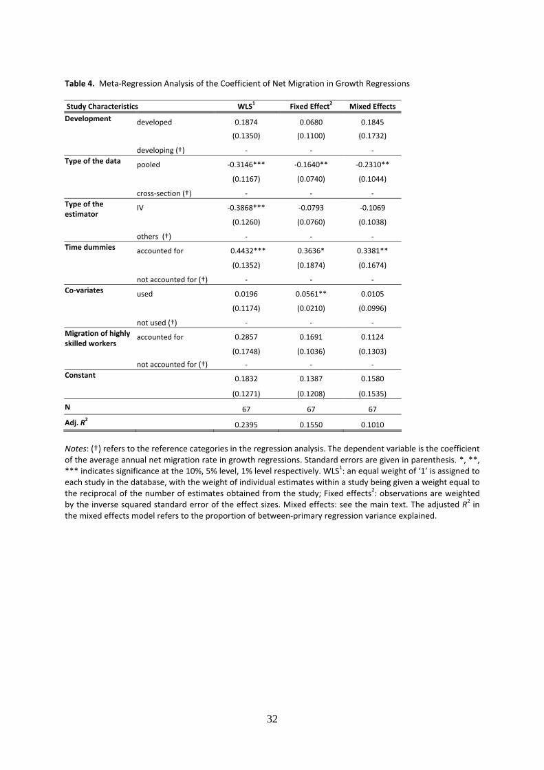
In meta‐regression analysis we can assess whether such study characteristics  jointly affect 

the mean  effect  size  in  a  statistically  significant way.  The  results  of  the meta‐regression 

model using different estimators are given  in Table 4. Since we have a modest number of 

observations, we aim  to  formulate a  straightforward model  that brings  further  insights  to 

methodological and empirical discussions. The reported regressions have been selected on 

grounds of theoretical considerations and goodness of fit. 

 

20

5.2. 1. Meta‐regression Analysis of the Coefficient of Net migration 

Table 2 shows that the mean estimate of the migration coefficient varies across a number of 

study  characteristics:  type of data,  type of estimator, etc. We  report our  results by using 

three estimation techniques that were discussed previously. These are the WLS, fixed effect 

and mixed effects models. The results are given in Table 4. Varying the estimators allows us 

to identify the robustness of the results. The results are in fact qualitatively highly consistent 

across  the  three  approaches.  Nonetheless,  it  is  not  realistic  to  expect  meta‐analysis  to 

explain the entire variation that exists in the data (Nelson and Kennedy, 2008). The outcome 

of  empirical  testing  cannot  be  predicted  beforehand,  precisely  because  the  sources  of 

influence on  the outcome are both numerous and sometimes unidentifiable  (Raudenbush, 

1994).  

 

Table 4 about here 

 

Heterogeneity  and  quality  variation  of  data  are  important  issues  that  affect  empirical 

estimates and  therefore meta‐analysis.  In general,  there  is a consensus  that  regional scale 

data  are more  homogenous  compared with  cross‐country  data  (Barro  and  Sala‐i Martin, 

1992; Abreu et al., 2005). However,  in countries within which  regional disparities are very 

high or the data of lesser quality, estimates may be affected by this. Additionally, the level of 

development  may  have  an  impact  on  the  role  of  migration  in  growth  regressions.  For 

instance, in developing countries migration would be more homogeneous than in developed 

countries. The migration that takes place  in the developing world  is predominantly rural to 

urban, while migrants of the developed world have a tendency to move between cities witin 

and between countries in the same part of the world. This contributes to agglomeration and 

its positive impact on growth (World Bank, 2008b). Table 4 shows that the dummy variable 

for development has a positive coefficient in the meta‐regression models, but the coefficient 

is not statistically significant.  

 

There  are  two  important  econometric  issues  in  the  migration  and  growth  literature: 

simultaneity bias, and omitted variable bias (OVB) (Kırdar and Saraçoğlu, 2008). Areas with 

higher  than  average  real  wage  growth  are  expected  to  exhibit  relatively  strong  net  in‐

migration flows. There is therefore a two‐way causality between growth and migration. For 

21

this reason, OLS may generate biased estimates. Thus, the use of two stage models such as 

2SLS  and  IV  is highly  recommended  in  the  literature.  Table  4  suggests  that  IV  estimation 

leads to a reduction in the positive effect of migration on real income growth. However, this 

effect is statistically significant only in WLS estimation. 

 

In the presence of omitted variable bias  (OVB), there  is a correlation between unobserved 

regional characteristics and growth. Using a panel structure with regional fixed effects is one 

way  in  which  researchers  can  overcome  OVB  (as  long  as  the  omitted  variable  is  cross‐

sectional  rather  than  temporal).  Hence,  a  panel  data  methodology  controls  for  time‐

invariant  structural  differences  across  the  regions  (Cashin  and  Loayza,  1995;  Etzo,  2008). 

Table 4 shows that using pooled data decreases the effect of migration on growth, and this is 

the case for all meta‐regression estimators (significant at the 5 percent level).  

 

The  heterogeneity  of  migrants  is  an  important  recent  issue  in  the  literature.  The  skill 

composition  of  the migrants may  directly  affect  the  impact  on  host  regions  (Etzo,  2008; 

Shioji,  2001).  Highly‐skilled migrants  are  expected  to  have  a  stronger  positive  impact  on 

growth than lesser‐skilled migrants. They are also more mobile. Researchers are increasingly 

questioning  the measurement  of migrants’  skills,  and  are  suggesting  that  gross migration 

rates  should be  studied  rather  than net migration  rates because of asymmetric effects of 

skills on  inward and outward migration.  It  is therefore  important to consider those studies 

that have controlled for the composition of migrants.17 In our meta‐sample, only studies on 

Italy  and  Japan  have  considered  highly  skilled migrants  as  an  explanatory  variable. We 

accounted  for  the composition effect with a migrant‐skill dummy, which  turned out  to be 

positive in all three models, but which was statistically insignificant.  

 

Various covariates are included in growth regressions to avoid omitted variable bias. Sectoral 

composition  and  per  capita  public  investment  are  among  the  most  frequently  used 

covariates. The sectoral composition variable provides a measure of how the endowment of 

industries  in a  region affects overall growth  (i.e., whether  sunrise or  sunset  industries are 

17 The human capital embodied in a migrant worker with a low educational attainment, but with a high level of work  experience,  is  likely  to  be  underestimated when only  education  is  taken  into  account.  Common  data deficiencies are a major obstruction to further analysis along these lines. 

22

overrepresented.  See  Cardenas  and  Ponton,  1995).  The  effect  of  the  inclusion  of  such 

covariates appears  to have a positive effect on  the estimated coefficient of net migration, 

but the effect is only statistically significant in the case of the fixed effect model. 

 

In measuring  the consequences of migration,  it  is  important  to allow  for exogenous  shifts 

and  trends  such  as  technological  improvements.  Such  forces  could  create  temporary  or 

permanent migratory waves.  In such cases,  it would be wise  to consider a  time dummy  in 

the primary growth regression since the estimate of the migration impact may otherwise be 

biased. We  find  a  positive,  and  statistically  significant,  effect  of  between  0.3  and  0.4  for 

studies that allowed for time dummies. 

 

5.2.2.  Meta‐regression  Analysis  on  the  Difference  in  Beta  Coefficients  with  and  without 

Migration 

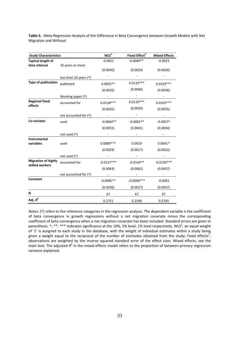
Table 5  reports some  results of meta‐regression analysis on  the  impact of a net migration 

variable  in  growth  regressions  on  the  estimated  coefficient  of  beta  convergence.  The 

estimators that are compared are the same ones as in Table 4. The dependent variable is the 

coefficient  of  beta  convergence  in  growth  regressions without  a  net migration  covariate 

minus the corresponding coefficient of beta convergence when a net migration covariate has 

been  included.  If  a  study  characteristic makes  this  difference more  positive,  it  leads  to 

greater  support  for  the neoclassical model, whereas  if  the  study  characteristic makes  the 

difference  more  negative,  it  tends  to  be  more  supportive  of  net  migration  reinforcing 

economic growth (see again Figure 3). The reported models have been selected on grounds 

of relative goodness of fit or a priori plausibility of the results. 

 

Table 5 about here 

 

The time span of the data used in the estimations in primary studies is an important variable 

in convergence analysis. Beta convergence is a long‐run process that can only be estimated 

with  data  over  a  long  time  span,  to  avoid  business  cycles  biasing  the  estimate.  The  bias 

introduced by omitting a net migration variable in the regression may also be affected by the 

time  span of  the data.  Table 5  shows  that  a  longer  time  frame  is needed  to  capture  the 

23

neoclassical growth process: the time  interval dummy has a statistically significant positive 

coefficient, but only in the fixed effect model. 

 

Although  we  did  not  find  publication  bias  among  the  selected  studies  (see  section  4.3 

above),  there  is  a  possibility  that  studies  published  in  journal  articles  find  on  average  a 

different  effect  from  non‐refereed working  papers.  Table  5  shows  that  this  is  indeed  the 

case. Published  studies  report more positive  values  for  the difference  in estimated betas, 

suggesting that the non‐orthodox (neoclassical)  interpretation  is more common among the 

working papers. 

 

The  primary  studies  included  in  the meta‐sample  refer  to  regions  across  a wide  array  of 

countries. Regional fixed effects may capture the unobserved heterogeneity of various socio‐

economic differences between the regions. The speed of convergence increases if we allow 

for higher  level of  regional variation  (Kırdar and Saraçoğlu, 2008).  Including  regional  fixed 

effects  provides  arguably  better  specified  growth  regressions  and  shifts  the  difference  in 

beta  coefficients  upwards.  The  results  suggest  indeed  that  introducing  a  net  migration 

variable  in the growth model has an  impact on beta that  is about 1 percentage point more 

positive when  regional  fixed effects are used  than when  they are not. The effect  is highly 

significant in all three models.  

 

The  inclusion of  additional  covariates  in  growth  regressions  controls  for  the possibility of 

spatial differences  in steady state growth path, and bias  in estimates of beta convergence 

(Abreu  et  al.,  2005).  Once  such  variables  are  included,  the  impact  of  the  net migration 

variable on the difference in betas becomes more negative. 

 

As noted previously, the endogeneity of net migration  in growth regressions  (migrants are 

disproportionally  attracted  to  the  fastest  growing  regions,  leading  to  a  high  correlation 

between  net migration  and  growth)  can  be  accounted  for  by means  of  the  instrumental 

variables  technique  (Barro  and  Sala‐i  Martin,  2004).  Table  5  confirms  that  using  an 

instrument  slightly  increases  the  difference  between  betas with  and without  a migration 

variable. However, the coefficient is statistically insignificant in the fixed effect model.  

 

24

As in Table 4, we also examine again the effect of the measured skill level of migrants on the 

growth  regression. We  have  seen  that  the  introduction  of  the  net migration  variable  on 

average increases the role of initial income (i.e. beta convergence) in explaining growth, and 

if the net migration variable refers to highly skilled migrants only, the (negative) difference 

between  the  estimated  speed  of  convergence  without  and  with  the  migration  variable 

appears  to  become  even  greater,  and  the  effect  is  statistically  significant  across  all  three 

estimators. 

 

Finally, the results reported in Tables 4 and 5 did not exploit the fact that each observation 

in  the  two meta‐regression  analyses  came  from  the  same  primary  regression.  The  error 

terms of  the model  for  the net migration  rate may  therefore be correlated with  the error 

terms of the model for the differences  in betas and these correlations can be exploited by 

means of  the  Seemingly Unrelated Regression  (SUR) model estimator  (e.g.  Zellner, 1962). 

The SUR approach was applied  to  the WLS model of Tables 4 and 5. However,  the  results 

were very similar to those already discussed. To save space they are not included.18

 

6. Conclusion 

In  this  study  the  issues of  comparability and  combinability of evidence, which need  to be 

considered  in  any  review,  have  been  made  explicit.  The  study  analysed  the  impact  of 

migration  on  income  growth  and  convergence  by  applying  several  meta‐analytical 

techniques which provided a quantitative methodological description  for, and measure of, 

effect  size heterogeneity  that exists  across  the primary papers.  The  results  appear  rather 

consistent  across  techniques.  However,  data  problems  –  particularly  regarding  the 

measurement of growth in regional income per capita and interregional migration over long 

time intervals – have been a common difficulty for researchers. This has limited the number 

of directly comparable estimates. 

 

As  a  result of  synthesizing  the empirical work, we  conclude  that  the overall effect of net 

migration on growth in real income per capita is positive, but small. A one percentage point 

increase in the net migration rate (equivalent to a one percentage point increase in the rate 

of  population  growth)  increases  the  rate  of  growth  in  per  capita  income  by  about  0.1  18 The SUR estimates are available from the authors upon request. 

25

percentage points. In contrast, in a standard neoclassical framework of a constant returns to 

scale economy with a composite good being produced and  labour’s share of  income being 

70 percent, an increase in the growth in labour supply of 1 percentage point would decrease 

growth in per capita income by 0.3 percentage points. However, with perfect capital mobility 

this effect would be offset by a commensurate increase in the capital stock (of 1 percentage 

point) and growth  in real per capita  income would remain unchanged. A positive sign of a 

net  inward migration coefficient  in a  real  income growth  regression  is consistent with  the 

perspective  of  the  new  endogenous  growth  theories  and  the  new  economic  geography 

(which  emphasise  the  strengthening  benefits  of  agglomeration)  rather  than  with  the 

neoclassical model with homogenous labour (Fingleton and Fischer, 2008).  

 

Moreover, we  find  that  the  estimated  rate  of  beta  convergence  (the  rate  at which  the 

economy converges to its steady state growth path) is also on average increased somewhat 

by  introducing  net  inward  migration  in  the  growth  regression.  Without  net  migration, 

estimated  beta  (conditional)  convergence  is  around  2.7  percent  per  annum  across  our 

sample  of  studies.  The  inclusion  of  a  net migration  variable  increases  this  to  about  2.73 

percent.19

 

Furthermore,  our  results  suggest  that  the  nature  of  the  data  (pooled  data  versus  cross‐

section;  the  length  of  the  time  interval)  has  a  significant  influence  on  the  impact  of  the 

migration variable  in growth regressions. The results also highlight the  importance of two‐

stage  estimation  techniques  such  as  IV  estimation  to  overcome  the  two‐way  causality 

problem  in the relationship between migration and growth. The IV method reveals a  lower 

migration  effect  on  income  growth.  We  also  identify  the  importance  of  controlling  for 

unobserved  regional  heterogeneity  by  means  of  fixed  effects  estimation.  Finally,  the 

estimates of the impact of net migration on per capita income growth depend on the model 

specification, in terms of the selected covariates, including the use of time dummies. 

 

The nature of  the mechanisms  through which net migration  increases  real  income growth 

still  has  to  be  explored  in  further  primary  research.  The  impact  of migration  on  capital 

accumulation  and  technological  change  would  be  central  issues  in  this  context.  The  19 Based on Table 3, panels (b) and (d) respectively. 

26

composition of the migration flows  in terms of the age, skills and diversity of the migrants 

may  play  an  important  role  too.  Finally,  the  present  paper  has  focussed  only  on  internal 

migration, but the impact of migration on income growth and convergence is clearly also an 

important  topic  in  the  current  debate  on  the  desirability  and  sustainability  of  current 

immigration levels in developed countries. Further primary research, and subsequently some 

synthesis by means of meta‐analysis, may be expected in that context as well. 

 References Abreu M,  Florax,  RJGM,  de  Groot,  HLF  (2005)  A Meta‐Analysis  of  Beta‐Convergence:  The  Legendary  Two‐

Percent. Journal of Economic Surveys 19(3): 389‐420.  Barro RJ, Sala‐i Martin X (1992) Regional Growth and Migration: A Japan‐United States Comparison. Journal of 

the Japanese and International Economies, 6: 312‐346.  Barro RJ, Sala‐i Martin X (2004) Economic Growth. 2nd edition. MIT Press. Begg CB (1994) Publication bias. In: H Cooper, and LV Hedges (eds) The Handbook of Research Synthesis, New 

York, Russell Sage Foundation, 399‐409.  Borenstein M,  Hedges  LV,  Higgins  Dr  JPT,  Rothstein  HR  (2009)  Introduction  to Meta‐Analysis,  1st  Edition, 

Electronic Book , John Wiley and Sons Ltd., England Borjas, G.J.  (1999). The Economic Analysis of  Immigration,  In O. Ashenfelter and D. Card  (eds) Handbook of 

Labor Economics, North Holland, 1697‐1760. Cardenas M,  Ponton  A  (1995)  Growth  and  Convergence  in  Colombia:  1950‐1990,  Journal  of  Development 

Economics, 47: 5‐37. Cashin  P,  Loayza  N  (1995)  Paradise  Lost?  Growth,  Convergence  and Migration  in  the  South  Pacific.  IMF, 

WP/95/28. Cass D (1965) Optimum Growth in an Aggregative Model of Capital Accumulation. Review of Economic Studies, 

37 (3): 233‐240.  Cochran WG (1954) Some Methods For Strengthening The Common X2 Tests. Biometrics, 10: 417–451. Cushing  B,  Poot  J  (2004)  Crossing  the  Boundaries  and  Borders:  Regional  Science  Advances  in  Migration 

Modelling. Papers in Regional Science, 83: 317‐338. 

Dobson S, Ramlogan C, Strobl E  (2006) Why Do Rates of β‐Convergence Differ? A Meta‐Regression Analysis. Scottish Journal of Political Economy 53(2): 153‐173. 

Dominicis  de  L,  Florax  RJGM,  de  Groot  HLF  (2008).  A Meta‐Analysis  on  the  Relationship  between  Income Inequality and Economic Growth. Scottish Journal of Political Economy, (55) 5: 654‐682. 

Egger M, Smith GD, Scheider M, and Minder C (1997a) Bias in Meta‐analysis Detected by Simple Graphical Test. British Medical Journal, 316: 629‐34. 

Egger M, Smith GD, Phillips AN (1997b) Meta‐analysis: Principles and Procedures. British Medical Journal, 315: 1533‐1537. 

Engels EA, Schmid CH, Terinn N, Olkin I, Lau J (2000) Heterogeneity and Statistical Significance in Meta‐Analysis: An Empirical Study of 125 Meta‐Analyses. Statistics in Medicine, 19: 1707‐1728. 

Etzo I (2008) Internal Migration: A Review of the Literature. MPRA Paper No.8783. Fingleton B, Fischer MM (2008) Neoclassical Theory versus New Economic Geography; Competing Explanations 

of Cross‐Regional Variation in Economic Development. SSRN, NY (visited on 30/11/2008).  Fratesi  U,  Riggi  RM  (2007)  Does Migration  Reduce  Regional  Disparities?  The  Role  of  Skill‐Selective  Flows. 

Review of Urban and Regional Development Studies, 19 (1): 78‐102.  Fujita, M., and Thisse, J‐F, 2002, Economics of Agglomeration: Cities, Industrial Location, and Regional Growth, 

Cambridge University Press, Cambridge. 

27

Gallup JL, Sachs JD, Mellinger AD (1999) Geography and Economic Development. International Regional Science Review, 22 (2): 179–232. 

Gezici  F, Hewings GJD  (2004)  Regional  Convergence  and  the  Economic  Performance  of  Peripheral  Areas  in Turkey. Review of Urban and Regional Development Studies, 16 (2): 113‐132.  

Glaeser  EL,  Kallal HD,  Scheinkman  JA,  Shleifer A  (1992) Growth  in Cities.  Journal  of  Political  Economy,  100: 1126‐1151. 

Greenwood MJ, Hunt GL  (1989)  Jobs versus Amenities  in  the Analysis of Metropolitan Migration.  Journal of Urban Economics, 25: 1‐16.  

Greenwood MJ (1975) Research on International Migration in the United States: A Survey. Journal of Economic Literature, 13 (2): 397‐433. 

Hamermesh DS (2007) Replication in Economics. Institute for the Study of Labor (IZA), Discussion paper 2760, Bonn. 

Hedges LV (1994) Fixed Effects Models. In: Cooper H, and Hedges LV (eds) The Handbook of Research Synthesis, New York, Russell Sage Foundation, 285‐299.    

Hedges LV, Olkin I, (1985) Statistical Methods for Meta‐Analysis, Academic Press, Inc.  Huedo‐Medina T, Sanchez‐Meca J, Marin‐Martinez F, Botella J (2006) Assessing Heterogeneity in Meta‐analysis: 

Q‐statistic or  I2  index? Center for Health,  Intervention, and Prevention, CHIP Documents, University of Connecticut, USA. http://digitalcommons.uconn.edu/chip docs/19 (visited on 15/12/2008)  

Islam, N.  (2003) What Have We Learnt  from  the Convergence Debate?  Journal of Economic Surveys 17: 309‐362. 

Kanbur R, Rapoport H (2005) Migration Selectivity and the Evolution of Spatial Inequality. Journal of Economic Geography, 5: 43‐57. 

Kırdar MG, Saraçoğlu DS  (2008) Migration and Regional Convergence: An Empirical  Investigation  for Turkey. Papers in Regional Science 87 (4): 545‐566. 

Koetse MJ,  Florax RJGM, de Groot HLF  (2007) The  Impact of Effect  Size Heterogeneity on Meta‐Analysis: A Monte Carlo Experiment. Tinbergen Institute Discussion Paper, TI 2007‐052/3, Amsterdam. 

Koopmans TC (1965) On the Concept of Optimal Economic Growth. Cowles Foundation Paper 238, Pontificiae Academiae Scientiarum Scripta Varia, Yale University, USA.  

Lipsey MW, Wilson DB  (2001) Practical Meta‐Analysis. Applied Social Research Method Series, Vol. 49, Sage Publications. 

Maza A (2006) Migrations and Regional Convergence: The Case of Spain. Jahrbuch für Regionalwissenschaft 26: 191‐202.  

McCann P (2001) Urban and Regional Economics, Oxford Publishing. Molho I (1986) Theories of Migration: A Review, Scottish Journal of Political Economy, 33 (4): 396‐419. Nijkamp P (2009) Regional Development as Self‐Organized Converging Growth.  In G. Kochendorfer‐Lucius and 

B. Pleskovic (eds). Spatial Disparities and Development Policy, World Bank, Washington DC, 265‐281. Nijkamp  P  and  Poot  J  (1998)  Spatial  Spatial  Perspectives  on New  Theories  of  Economic Growth. Annals  of 

Regional Science 32(1): 7‐37. Nelson  JP, Kennedy PE  (2008) The Use  (and Abuse) of Meta‐Analysis  in Environmental and Natural Resource 

Economics: An Assessment. Pennsylvania State University, unpublished paper. Ostbye S, Westerlund O  (2007)  Is Migration  Important  for Regional Convergence? Comparative Evidence  for 

Norwegian and Swedish Counties, 1980‐2000. Regional Studies, 41 (7): 901–915. Peeters L (2008) Selective In‐migration and Income Convergence and Divergence across Belgian Municipalities. 

Regional Studies, 42 (7): 905‐921. Pekkala and Kangasharju (2001) The Effect of Migration on Regional Convergence: Short‐Run Versus Long‐Run.               Unpublished working paper (Requested from the authors).  Perssons J (1997) Convergence across The Swedish Counties, 1911‐1993. European Economic Review, 41: 1835‐ 

1852. Pissarides  CA, McMaster  I  (1990)  Regional Migration, Wages  and  Unemployment:  Empirical  Evidence  and 

Implications for Policy. Oxford Economic Papers, 42: 812‐831. 

28

Polese M (1981) Regional Disparity, Migration and Economic Adjustment: A Reappraisal. Canadian Public Policy, VII (4): 519‐525. 

Poot  J  (2008) Demographic  Change  and  Regional  Competitiveness:  The  Effects  of  Immigration  and  Ageing. International Journal of Foresight and Innovation Policy 4(1/2): 129‐145. 

Ramsey FP (1928) A Mathematical Theory of Saving. Economic Journal, 38 (152): 543‐559. Raudenbush WS (1994) Random Effects Models. In: H Cooper, and LV Hedges (eds) The Handbook of Research 

Synthesis, New York, Russell Sage Foundation, 302‐321. Rappaport  J  (2005) How Does Labor Mobility Affect  Income Convergence?.  Journal of Economic Dynamics & 

Control 29: 567‐581. Reichlin  P,  Rustichini  A  (1998)  Diverging  Patterns with  Endogenous  Labour Migration.  Journal  of  Economic 

Dynamics and Control, 22: 703‐728. Rosenthal R, DiMatteo MR (2001) Meta‐Analysis: Recent Developments in Quantitative Methods for Literature 

Reviews. Annual Review Psychology, 52: 59‐82. Shadish WR, Haddock CK  (1994) Combining Estimates of Effect Size.  In: Cooper H, and Hedges  LV  (eds) The 

Handbook of Research Synthesis, New York, Russell Sage Foundation, 261‐282. Solow, RM (1956) A Contribution to the Theory of Economic Growth. Quarterly Journal of Economics, 70:65‐94. Soto R, Torche A (2004) Spatial Inequality, Migration, and Economic Growth in Chile. Cuadernos De Economía, 

Vol. 41: 401‐424. Shioji E  (2001) Composition Effect of Migration and Regional Growth  in  Japan.  Journal of  the  Japanese and 

International Economies, 15: 29–49.  Stanley  TD  (2001) Wheat  from Chaff: Meta‐Analysis  as Quantitative  Literature Review,  Journal  of  Economic 

Perspectives, 15(3): 131‐150. Sterne JAC (ed.) (2009) Meta‐Analysis in Stata: An Updated Collection from the Stata Journal. Stata Press. Stouffer SA (1940)  Intervening Opportunities: A Theory Relating Mobility and Distance. American Sociological 

Review, 5(6): 845‐867. Sutton AJ, Abrams KR, Jones DR, Sheldon TA, Song F (2000). Methods for Meta‐Analysis  in Medical Research, 

Wiley Series in Probability and Statistics, John Wiley & Sons Ltd. England.  Thompson SG, Sharp SJ (1999) Explaining Heterogeneity in Meta‐Analysis: A Comparison of Methods”, Statistics 

in Medicine, 18: 2693‐2708. Toya  H,  Hosono  K, Makino  T  (2004)  Human  Capital, Migration,  and  Regional  Income  Convergence  in  the 

Philippines.  Institute  of  Economic  Research,  Hitotsubashi University  (Tokyo)  Discussion  Paper  Series, No.18. 

UN  (2009)  World  Population  Prospects:  The  2008  Revision  Department  of  Economic  and  Social  Affairs Population Division, ESA/P/WP.210, NY UNFPA  (2007)  State  of World  Population  2007, Unleashing  the  Potential  of Urban Growth, United Nations 

Population Fund, NY. Verbeek, M (2004) A guide to Modern Econometrics. 2nd edition. John Wiley & Sons, Ltd. England.  Williamson JG (1991) Inequality, Poverty, and History. Blackwell, Oxford. World Bank (2008a) Urban Growth Report: Strategies for Sustained and Inclusive Development, Commission on 

Growth and Development, Conference Edition World Bank (2008b) World Development Report 2009: Reshaping Economic Geography, World Bank Group Zellner, A (1962) An Efficient Method of Estimating Seemingly Unrelated Regression Equations And Tests For  

Aggregation Bias. Journal of the American Statistical Association, 57: 348–368 

29

Table 1. Primary Studies used in the Meta‐analysis 

  Table 2. Descriptive Statistics for the Coefficient of Net Migration in Growth Regressions 

 (*)stands for the reference categories in regression analysis 

      

30

 Table 3. Fixed and Random Effects Estimates  (a) The coefficient of the net migration rate in growth regressions  Method  Pooled Estimate  95% CI LB  95% CI UB 

Fixed  0.092  0.086  0.099 Random  0.133  0.099  0.168 

Test for heterogeneity: Q = 336.27 with 66 degrees of freedom (p=0.000)   (b) The beta convergence coefficient in regressions without a net migration rate  Method  Pooled Estimate  95% CI LB  95% CI UB 

Fixed  0.030  0.030  0.031 Random  0.027  0.025  0.030 

Test for heterogeneity: Q = 714.24 with 66 degrees of freedom (p=0.000)   (c) The beta convergence coefficient in regressions with a net migration rate  Method  Pooled Estimate  95% CI LB  95% CI UB 

Fixed  0.005  0.005  0.005 Random  0.029  0.025  0.034 

Test for heterogeneity: Q = 5358.66 with 66 degrees of freedom (p=0.000)  (d) The pairwise difference in beta convergence coefficients  Method  Pooled Estimate  95% CI LB  95% CI UB 

Fixed   0.0006  0.0001  0.0011 Random  ‐0.0003  ‐0.0021  0.0016 

Test for heterogeneity: Q = 469.10 with 66 degrees of freedom (p=0.000)       

31

 Table 4.  Meta‐Regression Analysis of the Coefficient of Net Migration in Growth Regressions   Study Characteristics  WLS1 Fixed Effect2 Mixed Effects 

Development  developed  0.1874  0.0680  0.1845     (0.1350)  (0.1100)  (0.1732)   developing (†)  ‐  ‐  ‐ Type of the data  pooled  ‐0.3146***  ‐0.1640**  ‐0.2310**     (0.1167)  (0.0740)  (0.1044)   cross‐section (†)  ‐  ‐  ‐ 

IV  ‐0.3868***  ‐0.0793  ‐0.1069 Type of the estimator 

  (0.1260)  (0.0760)  (0.1038)   others  (†)  ‐  ‐  ‐ Time dummies  accounted for     0.4432***  0.3636*  0.3381**     (0.1352)  (0.1874)  (0.1674)   not accounted for (†)   ‐  ‐  ‐ Co‐variates  used  0.0196  0.0561**  0.0105     (0.1174)  (0.0210)  (0.0996)   not used (†)  ‐  ‐  ‐ 

accounted for   0.2857  0.1691  0.1124 

  (0.1748)  (0.1036)  (0.1303) 

Migration of highly   skilled workers 

not accounted for (†)   ‐  ‐  ‐ Constant    0.1832   0.1387  0.1580       (0.1271)  (0.1208)  (0.1535) 

N    67  67  67 

Adj. R2  0.2395  0.1550  0.1010 

 Notes: (†) refers to the reference categories in the regression analysis. The dependent variable is the coefficient of the average annual net migration rate in growth regressions. Standard errors are given in parenthesis. *, **, *** indicates significance at the 10%, 5% level, 1% level respectively. WLS1: an equal weight of ‘1’ is assigned to each study in the database, with the weight of individual estimates within a study being given a weight equal to the reciprocal of the number of estimates obtained from the study; Fixed effects2: observations are weighted by the inverse squared standard error of the effect sizes. Mixed effects: see the main text. The adjusted R2 in the mixed effects model refers to the proportion of between‐primary regression variance explained.     

32

 Table 5.  Meta‐Regression Analysis of the Difference in Beta Convergence between Growth Models with Net Migration and Without    Study Characteristics  WLS1 Fixed Effect2 Mixed Effects 

Typical length of time interval  10 years or more 

‐0.0022  0.0049**  ‐0.0023 

    (0.0030)  (0.0024)  (0.0026) 

  less than 10 years (†)  ‐  ‐  ‐ 

Type of publication  published  0.0092**  0.0133***  0.0103***     (0.0035)  (0.0040)  (0.0036)   Working paper (†)  ‐  ‐  ‐ 

accounted for  0.0118***  0.0110***  0.0103*** Regional fixed effects 

  (0.0035)  (0.0039)  (0.0035)   not accounted for (†)  ‐  ‐  ‐ 

Co‐variates  used     ‐0.0064**  ‐0.0082**  ‐0.0057*     (0.0031)  (0.0041)  (0.0034)   not used (†)   ‐  ‐  ‐ Instrumental variables  used  0.0089***  0.0019  0.0041*     (0.0029)  (0.0017)  (0.0022)   not used (†)  ‐  ‐  ‐ 

accounted for   ‐0.0137***  ‐0.0144**  ‐0.0136*** 

  (0.0043)  (0.0062)  (0.0037) 

Migration of highly skilled workers 

not accounted for (†)   ‐  ‐  ‐ Constant    ‐0.0085**  ‐0.0090***  ‐0.0055       (0.0036)  (0.0027)  (0.0037) 

N    67  67  67 

Adj. R2  0.2751  0.2598  0.3793 

 Notes: (†) refers to the reference categories in the regression analysis. The dependent variable is the coefficient of  beta  convergence  in  growth  regressions  without  a  net  migration  covariate  minus  the  corresponding coefficient of beta convergence when a net migration covariate has been included. Standard errors are given in parenthesis. *, **, *** indicates significance at the 10%, 5% level, 1% level respectively. WLS1: an equal weight of  ‘1’  is assigned to each study  in the database, with the weight of  individual estimates within a study being given a weight equal  to  the  reciprocal of  the number of estimates obtained  from  the  study;  Fixed effects2: observations are weighted by  the  inverse  squared  standard error of  the effect  sizes. Mixed effects:  see  the main text. The adjusted R2 in the mixed effects model refers to the proportion of between‐primary regression variance explained.   

33

 Figure 1: Quantile plot of the distribution of the coefficients of net migration rates in growth regressions  

-10

12

Qua

ntile

s of

coe

ff of

ann

ual a

ve n

et m

ig

0 .25 .5 .75 1Fraction of the data

    Figure 2. Quantile plot of the difference in beta convergence in regressions without and with a net migration variable  

-.04

-.02

0.0

2.0

4Q

uant

iles

of b

o - b

i

0 .25 .5 .75 1Fraction of the data

    

34

  Figure 3. Scatter plot (and least squares regression line) of coefficients of the net migration rate and the corresponding difference in beta convergence in regressions without and with a net migration variable  

-.04

-.02

0.0

2.0

4

-1 0 1 2coeff of annual ave net mig

Fitted values bo - bi

   Figure 4. Funnel plot for publication bias in reported estimates of net migration rates in growth regressions  

01

23

stan

dard

erro

r of c

oeff

of a

nnua

l ave

net

mig

-5 0 5coeff of annual ave net mig

Funnel plot with pseudo 95% confidence limits

  

35

  Figure 5. Funnel plot for publication bias in reported estimates of the difference in beta convergence between including and excluding a net migration rate in growth regressions  

0.0

05.0

1.0

15.0

2s.

e. o

f bom

inus

bi

-.04 -.02 0 .02 .04bo - bi

Funnel plot with pseudo 95% confidence limits

    

36