48
The effect of own and spousal parental leave on earnings Elly-Ann Johansson WORKING PAPER 2010:4
The effect of own and spousal parental leave on earnings
Elly-Ann Johansson
WORKING PAPER 2010:4

The Institute for Labour Market Policy Evaluation (IFAU) is a research institute under the Swedish Ministry of Employment, situated in Uppsala. IFAU’s objective is to promote, support and carry out scientific evaluations. The assignment includes: the effects of labour market policies, studies of the functioning of the labour market, the labour market effects of educational policies and the labour market effects of social insurance policies. IFAU shall also disseminate its results so that they become acces-sible to different interested parties in Sweden and abroad. IFAU also provides funding for research projects within its areas of interest. The deadline for applications is October 1 each year. Since the researchers at IFAU are mainly economists, researchers from other disciplines are encouraged to apply for funding. IFAU is run by a Director-General. The institute has a scientific council, consisting of a chairman, the Director-General and five other members. Among other things, the scientific council proposes a decision for the allocation of research grants. A reference group including representatives for employer organizations and trade unions, as well as the ministries and authorities concerned is also connected to the institute. Postal address: P.O. Box 513, 751 20 Uppsala Visiting address: Kyrkogårdsgatan 6, Uppsala Phone: +46 18 471 70 70 Fax: +46 18 471 70 71 [email protected] www.ifau.se Papers published in the Working Paper Series should, according to the IFAU policy, have been discussed at seminars held at IFAU and at least one other academic forum, and have been read by one external and one internal referee. They need not, however, have undergone the standard scrutiny for publication in a scientific journal. The purpose of the Working Paper Series is to provide a factual basis for public policy and the public policy discussion. ISSN 1651-1166
IFAU – The effect of own and spousal parental leave on earnings 1
The effect of own and spousal parental leave on earnings*
by
Elly-Ann Johansson#
22 March 2010
Abstract This paper investigates the effect of parental leave – both own and spousal – on subse-quent earnings using different sources of variation. Using fixed-effect models, and in line with previous results, parental leave is found to decrease each parent’s future earn-ings. Also spousal leave is important, but only for mothers. In fact, each month the fa-ther stays on parental leave has a larger positive effect on maternal earnings than a sim-ilar reduction in the mother’s own leave. Using two reforms of the parental leave system as exogenous sources of variation yields only imprecisely estimated effects, even though the reforms had a strong effect on parental leave usage. However, the point es-timates tentatively suggest effects in the same range or larger than the fixed-effects model found.
Keywords: parental leave, gender equality, earnings JEL-codes: J13, J16, J24
* I wish to thank supervisors Peter Fredriksson and Per Johansson for excellent guidance. Helpful suggestions from Mikael Elinder, Jonas Lagerström, Håkan Selin, Björn Öckert and seminar participants at the Department of Economics, Uppsala university and participants at ELE conference on family economics in Lofoten are also acknowledged. # The Institute for Labour Market Policy Evaluation (IFAU), e-mail [email protected]
2 IFAU – The effect of own and spousal parental leave on earnings
Table of contents 1 Introduction ......................................................................................................... 3
2 The Swedish parental leave system and the reforms ........................................... 5
3 Identification ....................................................................................................... 6
4 Data ................................................................................................................... 134.1 Data and estimation ........................................................................................... 134.2 How the reforms affected parental leave use .................................................... 154.3 Exogeneity of reform exposure ......................................................................... 214.4 Preview of results – simple cross-tabulations ................................................... 25
5 Results ............................................................................................................... 285.1 Main results ....................................................................................................... 285.2 Robustness: other specifications ....................................................................... 31
6 Extensions ......................................................................................................... 326.1 Heterogeneous effects ....................................................................................... 326.2 The effect of non-holiday parental leave ........................................................... 326.3 Other outcomes: fertility and marital/cohabitation status ................................. 33
7 Concluding remarks .......................................................................................... 35
References ....................................................................................................................... 37
Appendix ......................................................................................................................... 41

IFAU – The effect of own and spousal parental leave on earnings 3
1 Introduction The last decades have seen a convergence in the labor market behavior of males and
females, where the male-to-female ratio of educational levels, participation rates, hours
worked and hourly earnings have declined (Lundberg and Pollak, 2007; Lundberg,
2005). Despite this, females continue to take the lion’s share of housework, child
minding and parental leave (Evertsson and Nermo, 2007; Gershuny and Robinson,
1988; Halleröd, 2005; Lundberg and Pollak, 2007), and it is sometimes argued that this
is one potential explanation for the remaining, unexplained earnings gap (Datta Gupta et
al, 2008; Lundberg and Pollak, 2007). For example, being on parental leave for young
children may reduce future earnings through a number of channels such as human capi-
tal losses during the absence period or signaling effects (Albrecht et al, 1999; Mincer,
1974; Mincer and Polachek, 1974; Mincer and Ofek, 1982; Stafford and Sundström,
1996).
An additional mechanism, generally ignored in previous work, is the effect via future
division of intra-household labor and child care. If parental leave today affects child
care and household labor tomorrow, also spousal parental leave may be an important
determinant of future earnings. For example, if a fathers’ parental leave helps him ac-
quire skills useful for taking care of children, this may affect future division of house-
work and child care within the family, and hence feed back onto maternal labor market
behavior. This paper investigates the effect of parental leave on earnings.1
1 The present study also serves to evaluate the Swedish daddy month reform. The main goals of the Swedish parental leave system are, as described in a government bill from 1993, gender equality, the child’s right to both parents, child development and equal opportunity for both males and females to combine parenthood with a career (The Swedish Government, 1994). To my knowledge, there are no studies on how the daddy month affected parental labor market behavior.
It fits into a
broader literature on the effects of career interruptions on earnings. However, the
present paper departs from previous studies in several ways. First, it explicitly investi-
gates the effect of not only own, but also spousal parental leave, an issue generally ig-
nored in previous work. Second, it utilizes several sources of variation to identify ef-
fects. Besides cross sectional (CS) and fixed-effects (FE) models, it utilizes two policy
4 IFAU – The effect of own and spousal parental leave on earnings
reforms of the Swedish parental leave system that produced arguably exogenous varia-
tion in parental leave. The reforms reserved one and two months of leave for each
spouse, which in practice decreased mothers’ leave (the first reform) and increased fa-
thers’ leave (both reforms). Since the new rules applied to parents with children born
after certain dates, the effect of reform exposure can be estimated using a difference in
differences (DD) or triple differences (DDD) strategy. Finally, the register-based data
set encompasses the entire Swedish population and is virtually free from missing-
variables problems, attrition and self-report errors.
Previous studies have mostly found negative effects on earnings of absence in gen-
eral and parental leave in particular (see for example Albrecht et al, 1999; Datta Gupta
and Smith, 2002; Gangl and Ziefle, 2009; Görlich and De Grip, 2009; Mincer, 1974;
Mincer and Polachek, 1974; Mincer and Ofek, 1982; Ruhm, 1998; Skyt Nielsen, 2009).
In general, regression adjustment approaches are used for identification, sometimes with
fixed effects to control for unobserved but time-invariant heterogeneity (Skyt Nielsen,
2009, is an exception using a reform of parental leave schemes among Danish publicly
employed as exogenous variation). Regarding the effect of spousal parental leave, this
issue is mostly ignored (one exception is Pylkkänen and Smith, 2003, who find that an
increased parental leave period for fathers (“fathers’ quota”) reduces the job absence
time of mothers, even when the days available for mothers are left unchanged). How-
ever, there are indications that early paternal involvement in childcare has effects on
their involvement also later on. For example, Nepomnyaschy and Waldfogel (2007) find
that fathers who take longer leave in connection to the birth of the child are more in-
volved in child-caring activities 9 months later. On the other hand, Ekberg et al (2004)
find no effects of ordinary parental leave on later care for sick children.
This paper shows that both own and spousal parental leave is potentially important
for future earnings. Using the fixed effects model to control for unobserved but time-
constant heterogeneity, the results show that each parent’s own leave has a significant
and negative effect on own future earnings. However, and more interesting, also spousal
leave is important, but only for mothers. Each month the father stays on parental leave
has a larger positive effect on maternal earnings than a similar reduction in the mother’s
own leave. Using the reforms as exogenous variation in parental leave yields imprecise

IFAU – The effect of own and spousal parental leave on earnings 5
estimates, despite the fact that both reforms strongly affected parental leave usage.
However, the point estimates tentatively suggest larger effects than what was found us-
ing the fixed effects model.
2 The Swedish parental leave system and the reforms
The modern Swedish parental leave system was introduced in 1974, when both parents
were given equal rights to use the system. It consists of several parts, the most important
one being the governmentally paid cash benefit for parents staying home to care for
their child. Most days (360 or 390, depending on child birth date) are reimbursed as a
percentage of the previous wage, while a smaller amount of days (90) are reimbursed on
a low flat rate. For individuals without the required previous labor market attachment,
all days are replaced on a fixed (low) flat rate. The number of days on cash benefits as
well as the reimbursement level has varied slightly over time; see Appendix for more
details. There is great flexibility in the parental leave cash benefits; they can be used
until the child turns eight years old and the parents can also choose to stay home part-
time. The leave is also job protected. For more information on the Swedish parental
leave system, see Berggren (2005), Duvander et. al. (2005) or The Swedish Social In-
surance Agency (2002).
The overwhelming majority of parental leave is taken by mothers (Batljan et al,
2004). To increase the fathers’ take up of parental leave benefits, two so called “daddy
months” were introduced, the first in 1995 and the second in 2002. Before 1995, each
parent were given half of the cash benefits days, but were free to transfer days to each
other. But for those with children born from the 1st of January, 1995, 30 days of cash
benefits are set aside for each parent and cannot be transferred. If those days are not
used, they are simply lost. The 1st of January, 2002, an additional daddy month was in-
troduced, making 60 days non-transferable. An important difference between the re-
forms is that in 1995, the total number of days was held constant, which meant that in
practice mothers lost one month of parental leave. In 2002, the total number of days in-
creased by one month so that mothers’ maximum number of days was left unchanged.

6 IFAU – The effect of own and spousal parental leave on earnings
It is important to note that the new rules apply according to the birth date of the child.
There are also other changes in the parental leave system and in the social insurance
system in general imposed from the 1st of January 1995 and the 1st of January 2002, but
they generally apply equally to all individuals regardless of child birth dates. Hence,
they affect both treatment (born after the turn of the year) and control (born after the
turn of the year) groups equally. There are, however, some exceptions. The reimburse-
ment rate was lowered from 90 to 80 percent in 1995. Although this affected all families
equally in the long run, parents with children born before 1995 were given a respite and
could keep their previous, higher replacement rate until the end of 1996. However, the
30 days set aside for each parent were excluded from this change and still replaced as 90
percent of previous wage. In 2002, the reimbursement rate for the flat rate days was
doubled and this only applied to children born after 1st of January, 2002.
The daddy month legislation applies only to parents with shared custody of the child.
Married parents are automatically given shared custody, while non-married parents
must apply for shared custody. However, the overwhelming majority of families have
shared custody. Within our sample (described below) 93 percent of all children had co-
habiting parents at the time they turned one, and among cohabiting parents shared cus-
tody is very common. For example, 96 percent of all cohabiting parents of 1-5 year old
children had shared custody in 1999 (Statistics Sweden, 2000). In the data, there is no
information on custodial arrangements.
3 Identification Theoretically, career interruptions and parental leave could affect an individual’s own
future earnings through three main channels. First is the effect via decreased market
human capital (Mincer, 1974; Mincer and Ofek, 1982). This loss in market human cap-
ital may arise for different reasons such as a) forgone experience, b) skill depreciation
during the leave, and c) effects ex ante via sorting into different types of jobs because of
anticipated future career interruptions (Gronau, 1988). Second, career interruptions may
work as a negative signal of work commitment (Albrecht et al, 1999; Datta Gupta and
IFAU – The effect of own and spousal parental leave on earnings 7
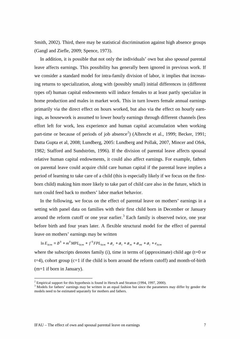
Smith, 2002). Third, there may be statistical discrimination against high absence groups
(Gangl and Ziefle, 2009; Spence, 1973).
In addition, it is possible that not only the individuals’ own but also spousal parental
leave affects earnings. This possibility has generally been ignored in previous work. If
we consider a standard model for intra-family division of labor, it implies that increas-
ing returns to specialization, along with (possibly small) initial differences in (different
types of) human capital endowments will induce females to at least partly specialize in
home production and males in market work. This in turn lowers female annual earnings
primarily via the direct effect on hours worked, but also via the effect on hourly earn-
ings, as housework is assumed to lower hourly earnings through different channels (less
effort left for work, less experience and human capital accumulation when working
part-time or because of periods of job absence2
In the following, we focus on the effect of parental leave on mothers’ earnings in a
setting with panel data on families with their first child born in December or January
around the reform cutoff or one year earlier.
) (Albrecht et al., 1999; Becker, 1991;
Datta Gupta et al, 2008; Lundberg, 2005: Lundberg and Pollak, 2007, Mincer and Ofek,
1982; Stafford and Sundström, 1996). If the division of parental leave affects spousal
relative human capital endowments, it could also affect earnings. For example, fathers
on parental leave could acquire child care human capital if the parental leave implies a
period of learning to take care of a child (this is especially likely if we focus on the first-
born child) making him more likely to take part of child care also in the future, which in
turn could feed back to mothers’ labor market behavior.
3
itcmimtmtcitcmitcmitcm eFPLfMPLmE ++++++++= aaaaab 000ln
Each family is observed twice, one year
before birth and four years later. A flexible structural model for the effect of parental
leave on mothers’ earnings may be written
where the subscripts denotes family (i), time in terms of (approximate) child age (t=0 or
t=4), cohort group (c=1 if the child is born around the reform cutoff) and month-of-birth
(m=1 if born in January).
2 Empirical support for this hypothesis is found in Hersch and Stratton (1994, 1997, 2000). 3 Models for fathers’ earnings may be written in an equal fashion but since the parameters may differ by gender the models need to be estimated separately for mothers and fathers.
8 IFAU – The effect of own and spousal parental leave on earnings
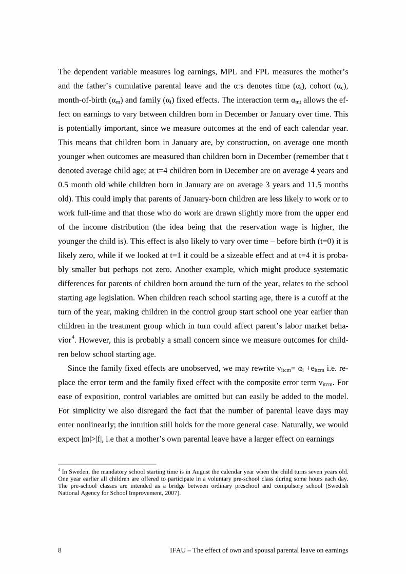
The dependent variable measures log earnings, MPL and FPL measures the mother’s
and the father’s cumulative parental leave and the α:s denotes time (αt), cohort (αc),
month-of-birth (αm) and family (αi) fixed effects. The interaction term αmt allows the ef-
fect on earnings to vary between children born in December or January over time. This
is potentially important, since we measure outcomes at the end of each calendar year.
This means that children born in January are, by construction, on average one month
younger when outcomes are measured than children born in December (remember that t
denoted average child age; at t=4 children born in December are on average 4 years and
0.5 month old while children born in January are on average 3 years and 11.5 months
old). This could imply that parents of January-born children are less likely to work or to
work full-time and that those who do work are drawn slightly more from the upper end
of the income distribution (the idea being that the reservation wage is higher, the
younger the child is). This effect is also likely to vary over time – before birth (t=0) it is
likely zero, while if we looked at t=1 it could be a sizeable effect and at t=4 it is proba-
bly smaller but perhaps not zero. Another example, which might produce systematic
differences for parents of children born around the turn of the year, relates to the school
starting age legislation. When children reach school starting age, there is a cutoff at the
turn of the year, making children in the control group start school one year earlier than
children in the treatment group which in turn could affect parent’s labor market beha-
vior4
Since the family fixed effects are unobserved, we may rewrite vitcm= αi +eitcm i.e. re-
place the error term and the family fixed effect with the composite error term vitcm. For
ease of exposition, control variables are omitted but can easily be added to the model.
For simplicity we also disregard the fact that the number of parental leave days may
enter nonlinearly; the intuition still holds for the more general case. Naturally, we would
expect |m|>|f|, i.e that a mother’s own parental leave have a larger effect on earnings
. However, this is probably a small concern since we measure outcomes for child-
ren below school starting age.
4 In Sweden, the mandatory school starting time is in August the calendar year when the child turns seven years old. One year earlier all children are offered to participate in a voluntary pre-school class during some hours each day. The pre-school classes are intended as a bridge between ordinary preschool and compulsory school (Swedish National Agency for School Improvement, 2007).

IFAU – The effect of own and spousal parental leave on earnings 9
than spousal parental leave. Previous research has generally ignored the spousal effects.
However, here we have the explicit aim to estimate also the effect of spousal parental
leave on own earnings.
First, if we only had cross-sectional data at t=4 the model would reduce to a standard
cross-sectional (CS) model,
icmimcicmicmicm eFPLfMPLmE ++++++= aaab 111ln (1)
which is consistently estimated by ordinary least squares as long as vicm=αi+eicm is un-
correlated with MPL and FPL. This assumption is unlikely to hold. For example, if par-
ents who take more (less) parental leave also are less (more) career oriented and for that
reason have lower (higher) earnings, this assumption is clearly violated. These differ-
ences in preferences for children versus market work may be difficult to proxy by in-
cluding standard control variables and the resulting estimates will reflect selection ra-
ther than causal effects. In such case, the estimates will be biased downwards. Another
possible story, potentially most applicable for fathers, is that fathers on leave – i.e. “re-
sponsible fathers” –are fathers with high earnings capacity. This interpretation is similar
to the male marital wage premium found in earlier literature, where married men and/or
fathers have higher earnings than non-married/non-fathers (Datta Gupta et. al, 2007;
Gray, 1997). This story would lead to an upward biased estimate of the effect of paren-
tal leave on earnings among fathers.
Previous studies have used individual/family fixed effects to control for unobserved
but time-invariant heterogeneity. If the endogenous variables – such as family prefe-
rences or “responsibility” – are constant over time, this approach yields unbiased esti-
mates. Given our panel data, we can estimate a dummy-variable fixed effects (FE)
model,
itcmimtcitcmitcmitcm eFPLfMPLmE +++++++= aaaab 222ln (2)
where we have assumed that αmt=0.5
5 Of course, we cannot distinguish between the different time-constant fixed effects, αc,αm and αi, they are estimated simultaneously.
Note that MPL and FPL are always zero before
birth so the main difference from model (1) above is that the dependent variable is
measured as first differences. Now, the family unobserved effect can be controlled for

10 IFAU – The effect of own and spousal parental leave on earnings
so this model is consistently estimated by OLS under the weaker assumption
E[Xitcm*∆eitcm]=0, where X=MPL, FPL. In particular, the model allows for fixed family
characteristics that are correlated with the dependent and independent variables.
However, to the extent that fertility (number, timing and spacing of children) is en-
dogenous, also fixed-effects models may yield biased estimates (Browning, 1992;
Lundberg, 2005). This could happen if, for example, fertility and/or parental leave re-
spond to income shocks. If so, we need some kind of exogenous variation in parental
leave to identify causal effects. This paper utilizes the daddy-month reforms as such
plausibly exogenous variation and compares children born just around the reform cu-
toffs. If we continue to assume αmt=0 – i e. that there are no time-varying systematic dif-
ferences between children born in December and January - we may restrict focus to
children born around the reform cutoff only (and exclude families with children born
the preceding year). Then a difference-in-differences (DD) model is given by
itmimtitmitm erREFORME +++++= aaab 3ln (3)
where REFORM is an indicator variable for being exposed to the reform. Note that this
variable is exactly the same as the interaction term between month-of-birth and time,
αmt, from above. This is why we need the αmt=0 assumption to hold in order for the
REFORM coefficient to measure the effect of the reform (rather than the effect of dif-
ferences between children born in December and January). If there are no such differ-
ences between children born in December and January, this model is consistently esti-
mated by OLS as long as E[REFORMitm*eitm]=0. In particular, exposure to the reform
should be exogenous and uncorrelated with for example income shocks. This specifica-
tion identifies the intention to treat (ITT) effect – the effect of the reform on all families
regardless of whether they comply or not – and as such, it mat be viewed as giving a
lower bound on the “true” effect of a month increase/decrease in parental leave for fa-
thers/mothers. In the absence of extra control variables, the reform coefficient equals the
difference between different group means, see Table 1.
If there are normal-year systematic differences between children born in December
and January (αtm≠0), for example because children in the group exposed to the reform
are slightly younger when earnings are measured, we would need to include also fami-

IFAU – The effect of own and spousal parental leave on earnings 11
lies from a comparison year and estimate a difference-in-difference-in-differences
(DDD) model,
itcmictmtmtcitcmitcm eREFORMrE ++++++++= aaaaaab 'ln 4 (4)
where REFORM=αctm now is an indicator for children born in January during reform
year at time t=4 (for completeness also the second “baseline” interaction effect αct is
added to the model). In the absence of control variables, also this REFORM coefficient
is given as a difference between group means; see Table 1 below.
Table 1 DD and DDD estimates
Comparison group
(child born one year before reform cutoff) Reform group
(child born around reform cutoff) Child’s month of birth December January December January lnE at t=0 a’ b’ a b lnE at t=4 c’ d’ c d Difference c’-a’ d’-b’ c-a d-b DD estimate (d’-b’)-(c’-a’) (d-b)-(c-a) DDD estimate [(d-b)-(c-a)]-[ (d’-b’)-(c’-a’)]
The models using the reforms as exogenous sources of variation (eq. 3-4) identifies
the joint effect of MPL and FPL for the first reform, and the effect of FPL for the
second reform. Remember that the second reform affected only fathers’ parental leave
while holding mothers’ available parental leave days constant. In contrast, the first
reform affected both parents’ leave; given that mothers before the reform used virtually
all parental leave, MPL was reduced by one month, while FPL was increased by a sim-
ilar amount for the compliers.
Using the first reform, and without further assumptions about the parameters (m and f) we
cannot identify whether the effect runs through own or spousal uptake of parental leave; we
have only one instrument and two endogenous variables. But since we have two reforms, it is, in
principle, possible to calculate instrumental variables estimates of the effect of each parent’s pa-
rental leave (rather than the “reduced form” reform effects). However, such a strategy requires
that there are no structural changes over time and since it is seven years between the first and
second reform, this assumption may be questioned. We may also note that by using the re-
forms as exogenous variation and comparing families around the reform cutoffs our
identification strategy isolates the direct and individual-level effect of parental leave on
earnings. In particular, the estimated effect does not include long-term equilibrium ef-

12 IFAU – The effect of own and spousal parental leave on earnings
fects, such as statistical discrimination, sorting into different types of job because of an-
ticipated future job absence, or increased female investments in market human capital
due to changed expectations of a future partner’s share of housework.
For simplicity the discussion above did not include control variables. Given ex-
ogeneity of treatment status, control variables X are unnecessary; the inclusion of con-
trol variables may, however, increase precision and is also an informal way of testing
exogeneity. Note, however, that the control variables are always measured prior to the
child’s birth and never in first differences even in the fixed-effects or DD/DDD models.
(In the standard fixed-effects setting, non-variant control variables drop out; however,
assuming that predetermined control variables can have different impact at different
times/child ages allows us to include interactions between time and the pre-determined
control variables.6
In the estimations, parental leave is measured only up to child age three (instead of
four). The reason is that the outcome is annual earnings (as compared to wages or
hourly earnings) and the prime purpose is to investigate the long-term effects of pre-
vious leave on future earnings (and not the obvious and immediate effect of parental
leave today on earnings today). See Section A2 in Appendix for more details on the
timing of variable collection.
)
As usual in earnings regressions, the problem of zeroes due to non-participation
arises since we only observe earnings for individuals who participate in the labor mar-
ket. Different processes may be at work on the extensive and intensive margin, and in-
cluding observations with value zero and using a linear estimation model may induce
specification bias due to nonlinearity. Focusing on individuals who do work necessarily
implies conditioning on an endogenous variable which yields a selected sample of par-
ticipants (Wooldridge, 2002). Throughout the paper OLS is used on log annual earnings
in SEK+1 to include also non-participants but results on the participation decision as
well as results for the participants only are shown in the Appendix.
6 Note that we never want to include control variables measured at t=4 since they may be affected by treatment and as such are part of the outcome.

IFAU – The effect of own and spousal parental leave on earnings 13
4 Data This section describes the data. It also describes how the reforms affected parental leave
usage and discusses issues of exogeneity.
4.1 Data and estimation The panel data set is based on register information (created by combining the LISA data
base and the so called multigenerational registry, provided by Statistics Sweden, with
data on parental leave provided by the Swedish Social Insurance Agency) encompassing
the entire Swedish population. It contains high-quality, individual level information on
all children and their family members, including information on annual earnings (from
the tax registers), parental leave usage and standard covariates such as age, educational
levels and marital status. There is in principle no attrition or missing variables problem.
The samples consist of native Swedish families7 whose first child8
The dependent variable measures log annual earnings (in SEK + 1 to include zero-
earners). The (possibly endogenous) independent variables of interest are the mother’s
and father’s total parental leave up to child age three. These are measured in days in the
descriptive section to give a precise picture of how the reforms affected parental leave,
but for readability they are rescaled to months (by dividing by 30) in the regressions.
These variables are used in models (1) and (2). The exogenous reform indicator, used in
was born one
month before or after each reform cutoff or the preceding year. Families whose first
birth was a multiple birth (approximately 3 percent) are excluded since the parental
leave rules for these families are slightly different. This leaves us with 9007 families for
the first reform sample and 8301 families for the second reform sample. In the main
analysis, most variables are observed both one year prior to the child’s birth (t=0) and
when the child is on average four years old (t=4); see Section 3 above and Section A2 in
Appendix for more details on the timing of data collection.
7 For immigrants, there are around 20% missing observation due to lack of educational information. However, including immigrants in the estimations does not change the results. 8 Only children who are both parents first-born child are included to avoid bias from previous children and their parental leave days.
14 IFAU – The effect of own and spousal parental leave on earnings
models (3) and (4), is 1 for children born in January 1995 (first reform sample) or Janu-
ary 2002 (second reform sample) and 0 for all other children. The models also include
the other indicator variables mentioned in Section 3 (cohort, month-of-birth, time and
their interactions). A number of control variables are also available, including parental
age and educational levels, marital status and child gender.
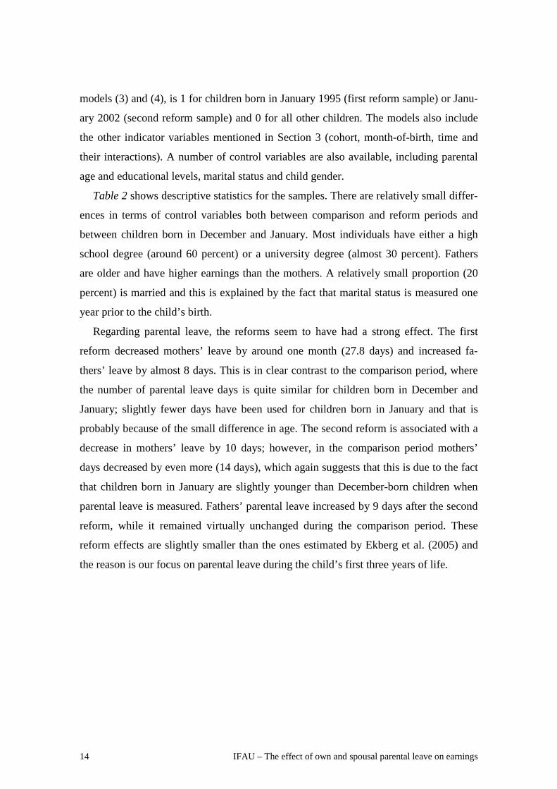
Table 2 shows descriptive statistics for the samples. There are relatively small differ-
ences in terms of control variables both between comparison and reform periods and
between children born in December and January. Most individuals have either a high
school degree (around 60 percent) or a university degree (almost 30 percent). Fathers
are older and have higher earnings than the mothers. A relatively small proportion (20
percent) is married and this is explained by the fact that marital status is measured one
year prior to the child’s birth.
Regarding parental leave, the reforms seem to have had a strong effect. The first
reform decreased mothers’ leave by around one month (27.8 days) and increased fa-
thers’ leave by almost 8 days. This is in clear contrast to the comparison period, where
the number of parental leave days is quite similar for children born in December and
January; slightly fewer days have been used for children born in January and that is
probably because of the small difference in age. The second reform is associated with a
decrease in mothers’ leave by 10 days; however, in the comparison period mothers’
days decreased by even more (14 days), which again suggests that this is due to the fact
that children born in January are slightly younger than December-born children when
parental leave is measured. Fathers’ parental leave increased by 9 days after the second
reform, while it remained virtually unchanged during the comparison period. These
reform effects are slightly smaller than the ones estimated by Ekberg et al. (2005) and
the reason is our focus on parental leave during the child’s first three years of life.

IFAU – The effect of own and spousal parental leave on earnings 15
Table 2 Descriptive statistics for the samples
Comparison cohort Reform cohort
Panel a) First reform sample Dec93 Jan94 Dec94 Jan95
Mother's earnings 117.8 118.8 112.5 111.3 (thousands SEK) (63.2) (64.2) (71.1) (71.5) Father's earnings 143.8 145.9 140.7 142.1 (thousands SEK) (89.5) (93.3) (105.3) (101.0) Mother’s PL (days) 460.4 457.8 467.1 439.3 (160.6) (154.6) (159.7) (152.5) Father’s PL (days) 50.1 47.5 40.4 47.9 (69.4) (69.7) (71.2) (62.0) Mother's age 25.6 25.6 25.6 25.5 (4.55) (4.40) (4.43) (4.42) Father's age 27.7 27.6 27.8 27.7 (4.96) (4.98) (4.94) (4.85) Mother w. high school educ. 0.60 0.59 0.59 0.61 Father w. high school educ. 0.58 0.60 0.60 0.58 Mother w. university educ. 0.29 0.29 0.29 0.28 Father w. university educ. 0.27 0.26 0.27 0.28 Married 0.18 0.17 0.18 0.18 Son 0.51 0.51 0.53 0.51 N 2135 2520 2115 2237
Panel b) Second reform sample Dec00 Jan01 Dec01 Jan02
Mother's earnings 155.3 155.8 170.0 170.4 (thousands SEK) (95.1) (99.4) (104.5) (105.7) Father's earnings 205.4 209.3 226.9 222.1 (thousands SEK) (128.4) (134.4) (176.7) (168.1) Mother’s PL (days) 408.1 394.4 405.3 395.2 (142.5) (142.6) (146.9) (138.8) Father’s PL (days) 56.6 57.3 62.5 71.6 (69.2) (68.5) (67.9) (69.7) Mother's age 26.8 26.9 27.3 27.0 (4.50) (4.58) (4.71) (4.55) Father's age 28.9 28.9 29.2 28.8 (5.01) (4.92) (5.04) (4.97) Mother w. high school educ. 0.50 0.48 0.54 0.56 Father w. high school educ. 0.54 0.53 0.66 0.64 Mother w. university educ. 0.38 0.40 0.38 0.36 Father w. university educ. 0.34 0.35 0.24 0.26 Married 0.21 0.20 0.20 0.18 Son 0.53 0.52 0.53 0.51 N 1848 2174 1944 2335 Notes: All variables except the parental leave variables and child gender are measured one year prior to the child’s birth. Earnings are measured in thousands SEK, including zeroes. Standard errors in parenthesis.
4.2 How the reforms affected parental leave use As a start, it is illuminating to look at how the reforms affected parental leave use from
different angles. Figure 1 starts by plotting the mean number of parental leave days
(measured at the end of the calendar years three years after the birth-turn of the year) for
different child birth month cohorts (December- or January-born children from different

16 IFAU – The effect of own and spousal parental leave on earnings
years). This shows the development of parental leave over time. Clearly, fathers’ pa-
rental leave increased at both reform cutoffs, while mothers’ parental leave decreased
only at the first reform cutoff. However, mothers with children born in January seem to
always have used slightly fewer parental leave days, most likely because their children
are on average one month younger when outcomes are measured. This small difference
in child age does not seem to affect fathers’ parental leave during non-reform years.
Figure 1 Mean parental leave for different child mob-cohorts
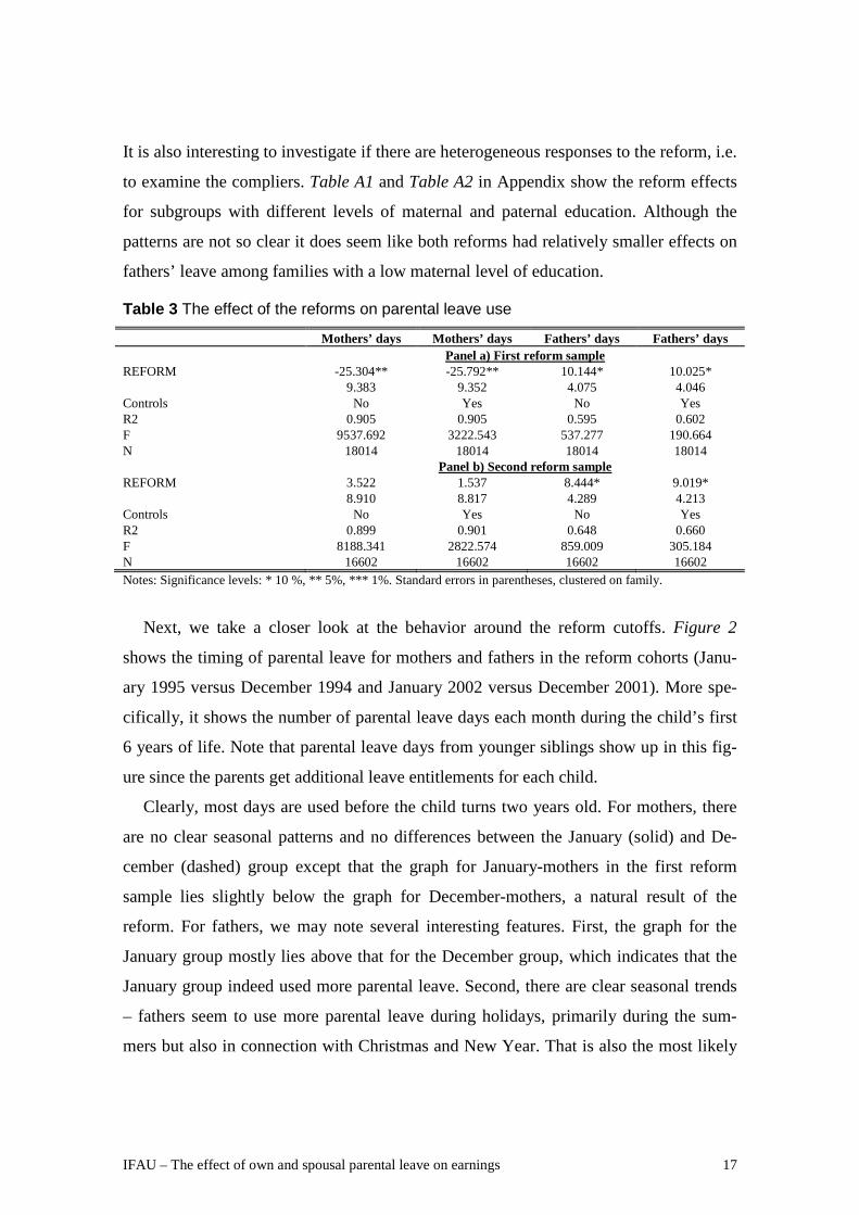
Second, Table 3 shows the results when parental leave days are regressed onto
reform exposure status with and without control variables (i.e. the DDD model (4)
above but with mothers’ and fathers’ days on parental leave instead of earnings as de-
pendent variable). Clearly, the reforms effectively increased fathers’ leave by around 9-
10 days each, and the first reform decreased mothers’ leave by almost 26 days. The
reform coefficients do not change much when control variables are added, which indi-
cates that the reforms were exogenous to the parents. However, this issue is more
deeply investigated in the Section 4.3 below.
IFAU – The effect of own and spousal parental leave on earnings 17
It is also interesting to investigate if there are heterogeneous responses to the reform, i.e.
to examine the compliers. Table A1 and Table A2 in Appendix show the reform effects
for subgroups with different levels of maternal and paternal education. Although the
patterns are not so clear it does seem like both reforms had relatively smaller effects on
fathers’ leave among families with a low maternal level of education.
Table 3 The effect of the reforms on parental leave use
Mothers’ days Mothers’ days Fathers’ days Fathers’ days REFORM
Panel a) First reform sample -25.304** -25.792** 10.144* 10.025*
9.383 9.352 4.075 4.046 Controls No Yes No Yes R2 0.905 0.905 0.595 0.602 F 9537.692 3222.543 537.277 190.664 N 18014 18014 18014 18014 REFORM
Panel b) Second reform sample 3.522 1.537 8.444* 9.019*
8.910 8.817 4.289 4.213 Controls No Yes No Yes R2 0.899 0.901 0.648 0.660 F 8188.341 2822.574 859.009 305.184 N 16602 16602 16602 16602 Notes: Significance levels: * 10 %, ** 5%, *** 1%. Standard errors in parentheses, clustered on family.
Next, we take a closer look at the behavior around the reform cutoffs. Figure 2
shows the timing of parental leave for mothers and fathers in the reform cohorts (Janu-
ary 1995 versus December 1994 and January 2002 versus December 2001). More spe-
cifically, it shows the number of parental leave days each month during the child’s first
6 years of life. Note that parental leave days from younger siblings show up in this fig-
ure since the parents get additional leave entitlements for each child.
Clearly, most days are used before the child turns two years old. For mothers, there
are no clear seasonal patterns and no differences between the January (solid) and De-
cember (dashed) group except that the graph for January-mothers in the first reform
sample lies slightly below the graph for December-mothers, a natural result of the
reform. For fathers, we may note several interesting features. First, the graph for the
January group mostly lies above that for the December group, which indicates that the
January group indeed used more parental leave. Second, there are clear seasonal trends
– fathers seem to use more parental leave during holidays, primarily during the sum-
mers but also in connection with Christmas and New Year. That is also the most likely

18 IFAU – The effect of own and spousal parental leave on earnings
explanation for the small difference in timing between January and December groups –
fathers in the January group are on parental leave slightly earlier and this may be be-
cause of the timing of holiday breaks. Apart from that, the differences between Decem-
ber and January groups are small.
Finally, Figure 3 shows the distribution of the amount of parental leave for January
(solid) and December (dashed) group, respectively. (In this figure, parental leave is
measured up to child age three – the variation that is used in the main analysis - but
looking at longer run parental leave does not change the overall picture). For the first
reform sample, the distribution of fathers’ days is clearly shifted to the right as a result
of the reform, with a new peak at around 30 days. The distribution of mothers’ days is
likewise shifted to the left (the peaks for mothers are located at or slightly below the
maximum available days on benefits, with and without the flat rate days). In this pic-
ture, the second reform does not seem to have affected mothers’ distribution of leave,
but fathers’ leave was again shifted to the right with a new peak at 60 days.

Figure 2 The timing of parental leave for reform cohorts by child month-of birth (December/January)

Figure 3 The distribution of parental leave days for reform cohorts by child month-of birth (December/January) Note: for visibility, the graph is cut at the one-child maximum of 450 days; however, a smaller amount of parents have used slightly more days than this since they had another child before the first child turned three.

IFAU – The effect of own and spousal parental leave on earnings 21
4.3 Exogeneity of reform exposure The parental leave reforms in 1995 and 2002 are used as exogenous sources of variation
in order to estimate the causal effect of parental leave on earnings. This identification
strategy requires that a) no other change, affecting treatment and control groups diffe-
rently, occurs at the same point in time as the reforms, and b) there is no endogenous
sorting at the reform thresholds.
Regarding (a), are the reforms the single changes affecting January and December
groups differently? Again, there were other changes in the social security system passed
the 1st of January in 1995 and 2002, but they generally affected both groups equally.
Only the daddy-month introduction along with some smaller changes in the reimburse-
ment rate for the transferable days (not the daddy-month) was tied to the birth date of
the child.
Regarding (b), is there any endogenous sorting at the reform thresholds? We start by
investigating static sorting, although it is worth noting that fixed individual characteris-
tics are allowed to be correlated with the probability of reform exposure (the individual
fixed effects are differenced out; see Section 3 above). However, if there are static sort-
ing it is also possible that there are sorting in terms of time-varying variables as well.
The first reform gave incentives for parents to induce an earlier birth, both to avoid
the daddy month restriction and because of the slightly higher replacement rate for
children born before 1995. The second reform reversely gave incentives to postpone
birth since the parental leave rules were strictly better for children born after the reform.
These incentives may have caused informed parents to fine-tune delivery. Are there
such indications?
The first reform was difficult to anticipate at the time of conception. Although the
daddy-month debate had been going on for years, it was unclear whether, when and how
it should be implemented. As late as the 26th of April, 1994, three parties from the go-
verning coalition threatened to vote against any such proposal (Karlsson, 1994a) and the
reform proposition was not passed until 30th of May, 1994 (Karlsson, 1994b) when the
turn of the year babies 1994/1995 were already conceived. Even so, parents could of
course plan an earlier birth just in case. In addition, although the exact natural birth date
is a random process it is in principle possible to induce an earlier birth by medical

22 IFAU – The effect of own and spousal parental leave on earnings
means, for example by using a caesarian section. The second reform had been known
long in advance (TT, 2001) and informed parents may have chosen to postpone child-
bearing.
Since there may be room for sorting around the reform cutoffs, we investigate this is-
sue a little deeper. First, Figure 4 below plots the number of first births in December
and January over time. There clearly seem to be large variations over time, and possibly
some tendencies of sorting in the anticipated direction – the difference in births between
January and December are relatively small in 1994/1995 and slightly larger in
2001/2002. However, such tendencies exist also at other points in time. In 1999/2000,
for example, the difference is even smaller than in 1994/1995.
Figure 4 Number of first births in December and January over time
Next, we investigate whether observables can explain treatment status. This may
show if there are indications of endogenous sorting at the reform cutoffs or if the pattern
in Figure 3 above is merely the result of random variation. (Of course, there could be
endogenous sorting that does not show up in terms of observables, but that is impossible
to investigate). Table 4 shows regression results when an indicator variable for being
exposed to the reform is regressed onto some arguably exogenous covariates (i.e. model
IFAU – The effect of own and spousal parental leave on earnings 23
(4) above but where the outcome variable is REFORM status and this is regressed onto
all other fixed effects and the control variables).
Clearly, there are no statistically significant differences in parental characteristics9
between children born in January and December and all point estimates are small in
magnitude10
Next, we investigate the more important issue, if there seems to be time-variant
sorting. In particular, we do not want reform exposure to be correlated with income
shocks. Instead, January and December groups should follow the same wage growth
paths over time.
. However, even if each single coefficient is statistically non-significant,
they could have explanatory power together. In fact, F-tests between these models and
similar models without control variables (only the fixed effects for cohort, time, month-
of-birth and their pairwise interactions are included) returns test statistics of 2.77 (first
reform sample) and 2.58 (second reform sample) which is statistically significant and
rejects the null hypothesis that the added control variables have no explanatory power.
So, there may be some static sorting in terms of observable characteristics. This sug-
gests that there could also be sorting in terms of unobservables. However, as noted
above, static sorting is in itself not problematic (since we have panel data and can esti-
mate the family fixed effects).
Table 5 investigates this issue by regressing the probability of reform
exposure (being born in January around the reform cutoff) on the fixed effects, the con-
trol variables and different earnings lags (maternal and paternal earnings two and three
years before the birth of the child). This is necessarily done on a slightly smaller sample
since these earnings lags are not available for all individuals. At most, we lose 74 indi-
viduals from the first reform sample and 75 individuals from the second reform sample.
Clearly, none of the earnings lags are statistically significant and they are also small in
magnitude. Hence, the groups exposed to the reforms seem to follow the same earnings
pattern over time as the comparison groups.
9 See also Ekberg et. al. (2005) who compare the number of births each day around the turn of the year 1994/1995 and other years and find no systematic pattern. In addition, they compare parental age distributions for children born two weeks before and after the reform and find no evidence of differences in parental characteristics. 10 All variables except the child gender variable are measured prior to the birth of the child.

24 IFAU – The effect of own and spousal parental leave on earnings
Table 4 The effect of exogenous characteristics on prob(reform exposure)
First reform Second reform Mother’s lnE (-0.002 0.002 (0.001) (0.002) Father’s lnE 0.001 -0.001 (0.001) (0.001) Father's age -0.000 -0.000 (0.001) (0.001) Mother's age -0.000 -0.001 (0.001) (0.001) Father w. high school educ. -0.012 0.003 (0.011) (0.013) Mother w. high school educ. 0.011 0.001 (0.013) (0.015) Father w. university educ. -0.000 0.015 (0.014) (0.015) Mother w. university educ. 0.005 -0.012 (0.015) (0.016) Married 0.002 -0.001 (0.010) (0.010) Son -0.005 -0.003 (0.007) (0.008) R2 0.857 0.872 F 1031.9 1329.9 N 18014 16602 Notes: All variables (except child gender) are measured one year before the birth of the child. Significance levels: * 10 %, ** 5%, *** 1%. Standard errors in parentheses, clustered on family.

IFAU – The effect of own and spousal parental leave on earnings 25
Table 5 The effect of income lags on prob(reform exposure)
Prob
(reform exposure) Prob
(reform exposure) Prob
(reform exposure) Prob
(reform exposure) Mother’s lnE, lag2
Panel a) First reform sample -0.001
(0.002) Mother’s lnE, lag3 -0.000 (0.002) Father’s lnE, lag2 0.002 (0.001) Father’s lnE, lag3 0.001 (0.001) Controls Yes Yes Yes Yes R2 0.857 0.857 0.857 0.857 F 1110.1 1089.9 1114.3 1111.0 N 17970 17866 17998 17970 Mother’s lnE, lag2
Panel b). Second reform sample 0.002
(0.001) Mother’s lnE, lag3 0.001 (0.001) Father’s lnE, lag2 -0.000 (0.001) Father’s lnE, lag3 -0.000 (0.001) Controls Yes Yes Yes Yes R2 0.872 0.872 0.872 0.872 F 1429.7 1403.4 1434.8 1427.8 N 16522 16452 16565 16533 Notes: Significance levels: * 10 %, ** 5%, *** 1%. Standard errors in parentheses, clustered on family.
4.4 Preview of results – simple cross-tabulations Without control variables, the REFORM-coefficient in the difference-in-differences
(DD) and triple differences (DDD) models can be calculated as simple differences be-
tween group means. Table 6 and Table 7 below shows these estimates for mothers and
fathers; both estimates are also shown for different placebo years and the DDD-esti-
mates are calculated using different comparison years. For ease of exposition, standard
errors are omitted but as will be clear from Section 5.1 the standard errors are indeed
huge and none of the differences below are statistically significant.
The first reform increased mothers’ subsequent earnings by 9 percent using the DD
approach and by 10-15 percent using the DDD approach with different comparison
years. Hence, it is a sizeable positive effect of the first reform on mothers’ earnings, and
the point estimate also seems robust to different comparison years. In addition, the DD-
and DDD-estimates from different placebo years are all much smaller and mostly of the

26 IFAU – The effect of own and spousal parental leave on earnings
reverse sign, which further indicates that the reform indeed had an effect on maternal
subsequent earnings. However, turning to the second reform, the results are less robust.
The coefficients from DD and DDD-models vary in both sign and size (from -5 percent
using the DD model to between 1 and 11 percent using DDD-models) and the result are
not very different from estimates in different pre-reform placebo years.
This could indicate that it is mothers’ own leave (which was affected by the first but
not the second reform) that is important. (Another possible story is that there could be
differences in parental leave timing between the reforms. Potentially the first reform in-
duced fathers to take more “non-holiday” parental leave, since otherwise the total ex-
pected leave was reduced, while the second reform was less strict in the sense that the
families were given an additional month of leave, implying that fathers could more
freely choose the timing of the parental leave. If so, and if “holiday”-parental leave is
less helpful for maternal labor market behavior, this could explain the difference in ef-
fects between the first and second reform.)
Regarding the fathers, both reforms seem to have had a negative effect on subsequent
earnings. The first reform’s estimates range from -18 to -34 percent, indeed huge effects
but suprisingly robust to the choice of comparison year and also more negative than any
of the pre-reform placebo estimates. The second reform’s estimates are much smaller, -5
to 5 percent, and also quite similar to the pre-reform placebo estimates.

IFAU – The effect of own and spousal parental leave on earnings 27
Table 6 Cross tabulations with DD and DDD estimates, mothers
Comparison cohort
3 Comparison cohort
2 Comparison cohort
1 Reform cohort
Panel a) First reform sample Dec 91
Jan 92
Dec 92
Jan 93
Dec 93
Jan 94
Dec 94
Jan 95
LnE at t=0 11,21 11,20 11,11 11,05 10,96 11,00 10,65 10,50 LnE at t=4 9,29 9,24 9,39 9,32 9,49 9,48 9,64 9,57 Diff -1,93 -1,96 -1,72 -1,73 -1,47 -1,53 -1,02 -0,93 DD estimate -0,03 -0,01 -0,06 0,09 DDD estimate1 0,02 -0,05 0,15 DDD estimate2 -0,03 0,10 DDD estimate3 0,12
Panel b) Second reform sample Dec 98
Jan 99
Dec 99
Jan 00
Dec 00
Jan 01
Dec 01
Jan 02
LnE at t=0 10,65 10,65 10,93 10,95 11,08 11,05 11,25 11,31 LnE at t=4 10,16 10,00 10,22 10,18 10,18 10,01 10,06 10,07 Diff -0,49 -0,65 -0,71 -0,77 -0,91 -1,05 -1,19 -1,24 DD estimate -0,16 -0,06 -0,14 -0,05 DDD estimate1 0,10 -0,08 0,09 DDD estimate2 0,02 0,01 DDD estimate3 0,11
Table 7 Cross tabulations with DD and DDD estimates, fathers
Comparison cohort
3 Comparison cohort
2 Comparison cohort
1 Reform cohort
Panel a) First reform sample Dec 91 Jan 92 Dec 92 Jan 93 Dec 93 Jan 94 Dec 94 Jan 95
LnE at t=0 11,21 11,24 11,14 11,15 10,87 10,82 10,39 10,55 LnE at t=4 10,98 11,10 11,04 11,10 11,18 11,05 11,26 11,18 Diff -0,24 -0,14 -0,10 -0,04 0,30 0,24 0,88 0,63 DD estimate 0,09 0,06 -0,07 -0,24 DDD estimate1 -0,04 -0,12 -0,18 DDD estimate2 -0,16 -0,30 DDD estimate3 -0,34
Panel b) Second reform sample Dec 98 Jan 99 Dec 99 Jan 00 Dec 00 Jan 01 Dec 01 Jan 02
LnE at t=0 10,93 10,91 11,05 11,16 11,29 11,34 11,51 11,38 LnE at t=4 11,58 11,48 11,46 11,59 11,50 11,58 11,68 11,53 Diff 0,64 0,57 0,42 0,43 0,21 0,24 0,17 0,15 DD estimate -0,07 0,01 0,03 -0,02 DDD estimate1 0,09 0,01 -0,05 DDD estimate2 0,10 -0,04 DDD estimate3 0,05
28 IFAU – The effect of own and spousal parental leave on earnings
5 Results
5.1 Main results Table 8 and show estimation results for mothers and fathers for the first and second
reform sample separately and using the different models (cross-section, fixed effects,
DD and DDD).
There are several things to note. First, there are clear differences between the cross-
sectional model and the fixed-effects model, which suggest selection of families into
different levels of parental leave usage. Second, using the fixed-effects model, own pa-
rental leave do seem to reduce subsequent earnings – each month of own parental leave
lowers mothers’ earnings by 4.5 percent (in the first reform sample) and fathers’ earn-
ings by around 7.5 percent. The magnitude of these effects is far larger than previous
studies – for example, Albrecht et al (1999) found wage reductions of 0.1-0.5 percent
for each month of parental leave. This can be explained by the fact that here, annual
earnings are used which reflect both wages and hours worked, while most previous stu-
dies have focused on wages. In addition, our focus is on the relatively short run effect
on earnings four years later, when some parents could still be on parental leave (and pa-
rental leave up to child age 3 may be correlated with later parental leave). In addition,
the longer-run effects are usually found to be smaller due to rebound effects and catch-
ing-up of human capital.
The differences in effects between males and females could be due to nonlinearities,
if the first months of leave are more important for earnings than later parental leave. It
could also be a signaling effect. As suggested by Albrecht et al (1999), parental leave
could have a stronger signaling value for males since so few fathers stay on parental
leave compared to virtually all mothers.
Third, and more interesting, spousal parental leave has no effect on father’s earnings
but do seem important for mother’s labor market behavior. Each additional month that
the father stays on parental leave increases mothers’ earnings by 6.7 percent in the first
reform sample (the effect in the second reform sample is not statistically significant).
This is a large effect, even larger than the effect of a mother’s own parental leave. This
indicates that paternal (lack of) involvement in parental leave and child care may in fact

IFAU – The effect of own and spousal parental leave on earnings 29
be one important explanation for the male-to-female earnings gap. Another story could
be a “reverse signaling” story – while most mothers take all available parental leave, a
shorter period of leave could work as a positive signal of work-commitment.
These causal interpretations rest on the assumption of no time-variant unobserved
heterogeneity, and in particular that fertility and parental leave is not endogenous. For
example, if parents who experience an income shock becomes more (less) likely to have
children and/or stay on parental leave, this assumption is clearly violated. Using the re-
forms as exogenous variation in parental leave do, unfortunately, yield very imprecise
estimates that are not statistically different from zero. We can note, however, that this is
not because of a weak effect on parental leave use. As we saw in Section 4.2, the reform
effectively changed the parents’ time on parental leave. Instead, it could be that the
normal-year variation in earnings depending on child birth dates is too large to enable
precise estimation.
However, we may still make some comparisons of the point estimates across models.
The tables also report the predicted reform effect for the CS/FE-models, which is a cal-
culation of the predicted effect of the reform if the assumptions underlying the CS or FE
models are fulfilled. This effect is calculated as the mean change in mothers’ and fa-
thers’ time on parental leave as induced by the reforms (see the reform-coefficient from
Table 2 above, columns 2 and 4), multiplied by the coefficient on each month of leave
as estimated by the CS/FE models.11
For example, if the fixed-effects results are true, we would expect the first reform to
increase maternal earnings by 6.1 percent; both because of the decrease in own leave
and because of the increase in spousal leave. This effect is well within the 95 percent
confidence interval of both models using the reform as exogenous variation. The most
flexible model, DDD, tentatively suggests even larger effects – the point estimate is
14.9, albeit very imprecisely estimated. The same pattern is found also for the second
reform sample and among fathers – model (4) always returns larger point estimates than
model (2). This tentatively suggests that the “true” effect is in the same range or larger
11 The standard error of this estimate is calculated assuming that the underlying variables are independent random variables.

30 IFAU – The effect of own and spousal parental leave on earnings
than suggested by the fixed-effects specification.
Finally, we can note that these estimates are quite similar to the estimates without
control variables (see the cross-tabulations above), which further indicates that the re-
forms are indeed exogenous.
Table 8 The effect of parental leave on mothers’ earnings at child age 4
CS FE DD DDD Mother's PL
Panel a) First reform sample -0.011 -0.045***
(0.009) (0.013) Father's PL 0.021 0.067* (0.019) (0.029) REFORM [0.017] [0.061] 0.088 0.149 [0.011] [0.023] (0.176) (0.244) Controls Yes Yes Yes Yes R2 0.059 0.656 0.667 0.655 F 40.717 45.833 17.038 41.939 N 9007 18014 8704 18014 Mother's PL
Panel b) Second reform sample 0.026** -0.023
(0.010) (0.014) Father's PL 0.034 0.036 (0.022) (0.030) REFORM [0.011] [0.010] -0.041 0.102 [0.012] [0.014] (0.164) (0.236) Controls Yes Yes Yes Yes R2 0.047 0.683 0.688 0.683 F 29.497 41.427 25.744 37.474 N 8301 16602 8558 16602 Notes: Significance levels: * 10 %, ** 5%, *** 1%. Standard errors in parentheses, clustered on family.

IFAU – The effect of own and spousal parental leave on earnings 31
Table 9 The effect of parental leave on fathers’ earnings at child age 4.
CS FE DD DDD Mother's PL
Panel a) First reform sample 0.013 0.000
(0.007) (0.011) Father's PL 0.035 -0.076** (0.019) (0.027) REFORM [0.000] [-0.025] -0.256 -0.186 [0.011] [0.018] (0.165) (0.221) Controls Yes Yes Yes Yes R2 0.058 0.706 0.706 0.706 F 39.912 11.074 10.795 11.139 N 9007 18014 8704 18014 Mother's PL
Panel b) Second reform sample 0.007 0.005
(0.008) (0.012) Father's PL 0.010 -0.075** (0.020) (0.026) REFORM [0.003] [-0.022] -0.050 -0.074 [0.007] [0.014] (0.138) (0.206) Controls Yes Yes Yes Yes R2 0.047 0.714 0.731 0.713 F 25.454 3.860 2.125 3.031 N 8301 16602 8558 16602 Notes: Significance levels: * 10 %, ** 5%, *** 1%. Standard errors in parentheses, clustered on family.
5.2 Robustness: other specifications In the main analysis above, the dependent variable is defined as log(earnings+1) to in-
clude also individuals who do not participate in the labor market. As discussed above,
this is not unproblematic and Table A3 and Table A4 in Appendix show alternative
specifications for the effect of parental leave/the reforms on the probability of having
nonzero earnings (the extensive margin) and on log earnings among those with earn-
ings>0, using the FE or DDD models.
The effect of parental leave on the participation decision is mostly not statistically
significant, but the effect on log earnings among those with earnings >0 follow the same
pattern as above – a negative effect of own parental leave and, for mothers, a positive
effect of spousal leave in the second reform sample. The magnitudes of the effects are,
as expected, smaller since now zero observations are excluded and part of the effect in

32 IFAU – The effect of own and spousal parental leave on earnings
the main analysis above was driven by individuals with zero earnings. Again, the DDD
model returns only imprecisely estimated effects. 12
6 Extensions
6.1 Heterogeneous effects Usually, career interruptions are believed to be more harmful for individuals in occupa-
tions requiring a high level of human capital input. Therefore, we may hypothesize that
both own and spousal parental leave is more important for parents with a high level of
education. Also, as we saw above, the responsiveness to the reforms differed slightly
between groups. However, estimating the models (FE/DDD) separately for subgroups
with different maternal and paternal levels of education yields mostly imprecisely esti-
mated effects that are not significantly different between the groups. This is most likely
because of the smaller sample sizes in the FE case.
6.2 The effect of non-holiday parental leave If there is an effect of fathers’ leave on mothers’ labor market behavior, one might hy-
pothesize that this effect should differ depending on the timing of this leave. In particu-
lar, the great flexibility of the Swedish parental leave (remember that the days can be
used until the child turns eight years old) also means that parents can use parental leave
instead of ordinary vacation, for example during summertime or around Christmas.
Such parental leave is potentially less helpful for mothers’ careers than parental leave
used when the other spouse is working.
Table 10 shows the effect of non-holiday parental leave, which is defined as parental
leave excluding leave in June, July or August. This is estimated using the fixed-effects
specification (model 2). Indeed, and in line with the hypothesis, non-holiday parental
leave seems to have a larger negative effect on own earnings than summertime leave,
and father’s non-holiday leave has a larger positive effect on maternal earnings than
12 In addition, using the models above (eq. 1-4) with earnings in levels (SEK, including zeroes) instead of in logs yields similar results as when earnings in logs are used, which indicates that the results are not sensitive to the logarithmic transformation.
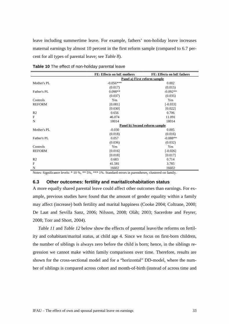
IFAU – The effect of own and spousal parental leave on earnings 33
leave including summertime leave. For example, fathers’ non-holiday leave increases
maternal earnings by almost 10 percent in the first reform sample (compared to 6.7 per-
cent for all types of parental leave; see Table 8).
Table 10 The effect of non-holiday parental leave
FE: Effects on lnE mothers FE: Effects on lnE fathers Mother's PL
Panel a) First reform sample -0.056*** 0.002
(0.017) (0.015) Father's PL 0.098** -0.092** (0.037) (0.035) Controls Yes Yes REFORM [0.081] [-0.033] [0.030] [0.022] R2 0.656 0.706 F 46.074 11.091 N 18014 18014 Mother's PL
Panel b) Second reform sample -0.030 0.005
(0.018) (0.016) Father's PL 0.057 -0.088** (0.036) (0.032) Controls Yes Yes REFORM [0.016] [-0.026] [0.018] [0.017] R2 0.683 0.714 F 41.581 3.785 N 16602 16602 Notes: Significance levels: * 10 %, ** 5%, *** 1%. Standard errors in parentheses, clustered on family.
6.3 Other outcomes: fertility and marital/cohabitation status A more equally shared parental leave could affect other outcomes than earnings. For ex-
ample, previous studies have found that the amount of gender equality within a family
may affect (increase) both fertility and marital happiness (Cooke 2004; Coltrane, 2000;
De Laat and Sevilla Sanz, 2006; Nilsson, 2008; Oláh; 2003; Sacerdote and Feyrer,
2008; Torr and Short, 2004).
Table 11 and Table 12 below show the effects of parental leave/the reforms on fertil-
ity and cohabitant/marital status, at child age 4. Since we focus on first-born children,
the number of siblings is always zero before the child is born; hence, in the siblings re-
gression we cannot make within family comparisons over time. Therefore, results are
shown for the cross-sectional model and for a “horizontal” DD-model, where the num-
ber of siblings is compared across cohort and month-of-birth (instead of across time and

34 IFAU – The effect of own and spousal parental leave on earnings
month of birth in the standard DD-model). For the regressions on cohabitant/marital
status, the FE and DDD-specifications are used.
Clearly, and in line with previous studies, both mothers’ and fathers’ parental leave
have positive effects on fertility and the probability of cohabiting and being married.
The coefficients in the cross-sectional and fixed-effects models are always statistically
significant and very close in magnitude over time (first versus second reform sample).
This suggests ambiguous expected effects of the first reform since it decreased mothers’
leave while increasing fathers’ leave, and positive effects of the second reform. Turning
to the DD/DDD models, the results are again imprecisely estimated, but the point esti-
mates for fertility are quite close to the predicted effects as suggested by the CS model.
Table 11 Effects on fertility (no. of younger siblings)
CS DD-variant Mother's PL
Panel a) First reform sample 0.057***
(0.001) Father's PL 0.065*** (0.002) REFORM [-0.028] -0.022 [0.020] (0.022) Controls Yes Yes R2 0.328 0.032 F 382.805 27.570 N 9007 9007 Mother's PL
Panel b) Second reform sample 0.052***
(0.001) Father's PL 0.055*** (0.002) REFORM [0.019] 0.011 [0.017] (0.023) Controls Yes Yes R2 0.272 0.057 F 272.253 45.510 N 8301 8301 Notes: Significance levels: * 10 %, ** 5%, *** 1%. Standard errors in parentheses, clustered on family.

IFAU – The effect of own and spousal parental leave on earnings 35
Table 12 Effects on cohabitant/marital status
Prob(cohabiting) Prob(married) FE DDD FE DDD Mother's PL
Panel a) First reform sample 0.010*** 0.010***
(0.001) (0.001) Father's PL 0.016*** 0.018*** (0.002) (0.003) REFORM [-0.003] -0.016 [-0.003] -0.008 [0.004] (0.021) [0.004] (0.025) Controls Yes Yes Yes Yes R2 0.878 0.875 0.794 0.791 F 2017.344 1653.074 179.212 160.217 N 18014 18014 18014 18014 Mother's PL
Panel b) Second reform sample 0.008*** 0.009***
(0.001) (0.001) Father's PL 0.016*** 0.020*** (0.002) (0.003) REFORM [0.005] -0.011 [0.007] -0.028 [0.003] (0.019) [0.004] (0.026) Controls Yes Yes Yes Yes R2 0.905 0.903 0.809 0.806 F 2897.678 2408.354 151.733 135.382 N 16602 16602 16602 16602 Notes: Significance levels: * 10 %, ** 5%, *** 1%. Standard errors in parentheses, clustered on family.
7 Concluding remarks This paper investigates the effect of parental leave on earnings. In contrast to most pre-
vious studies, not only own but also spousal parental leave is considered, under the hy-
pothesis that spousal help in child care may feed back onto each individual’s labor mar-
ket behavior.
Using a fixed effects model to account for time-constant unobserved heterogeneity,
the results show that own parental leave is associated with earnings reductions of 4.5
percent for mothers and 7.5 percent for fathers. In terms of sign, this is in line with pre-
vious studies. The size of the effects is much larger than in previous studies, partly be-
cause the focus here is on annual earnings (which also reflect hours worked) as com-
pared to wages, which is mostly used in other studies.
For mothers, also spousal parental leave is important for future earnings. Each month
that the father stays on parental leave increases maternal earnings by 6.7 percent, which
is an even larger effect than the mother’s own leave. This suggests that paternal (lack

36 IFAU – The effect of own and spousal parental leave on earnings
of) involvement in child care and parental leave could be one factor behind the remain-
ing, unexplained earnings gap. Among fathers, there is no effect of spousal parental
leave on earnings. Even larger effects of fathers’ leave on maternal earnings can be
found if we restrict focus to “non-holiday” parental leave, i.e. parental leave excluding
leave during the summer (June, July, or August). Such parental leave may be a better
measure of spousal help than parental leave during summertime (when both spouses
may be at home simultaneously because of ordinary vacation).
Finally, the fixed-effects model rests on the assumption of no unobserved, time-va-
riant heterogeneity. In particular, it assumes that parental leave is unaffected by for ex-
ample income shocks. If this assumption is violated, we need some kind of exogenous
variation to identify causal effects. The two daddy-month reforms in 1995 and 2002 had
a strong effect on parental leave usage. Despite that, using the reforms as exogenous
variation in parental leave yields only very imprecise estimates. This is most likely due
to large random variation in earnings depending on child birth dates. However, the point
estimates from DD and DDD models tentatively suggests effects in the same range or
larger than what was found using the fixed-effects specification.

IFAU – The effect of own and spousal parental leave on earnings 37
References Albrecht, J.W, P-A Edin, M. Sundström and S. B. Vroman (1999): Career interruptions
and subsequent earnings: a reexamination using Swedish data, The Journal of Human
Resources, vol. 34, no. 2
Batljan, I., S. Tillander, S. Örnhall Ljung and M. Sjöström (2004): Föräldrapenning,
pappornas uttag av dagar, fakta och analys, Ministry of Health and Social Affairs
(Socialdepartementet)
Becker, G. S. (1991): A treatise on the family. Enlarged edition. Cambridge, MA: Har-
vard university press
Berggren, S. (2005): An overview of the Swedish family benefits – goals and develop-
ments [in Swedish; English summary], working papers in social insurance 2005:1,
Swedish Social Insurance Agency
Browning, M. (1992): Children and household economic behavior, Journal of Economic
Literature, vol. 30, no. 3
Coltrane, S. (2000): Research on household labor: modeling and measuring the social
embeddedness of routine family work, Journal of Marriage and the Family, vol. 62,
no. 4
Cooke, L.P. (2004): The gendered division of labor and family outcomes in Germany,
Journal of Marriage and Family, vol. 66
Datta Gupta, N., N. Smith and M. Verner (2008): The impact of Nordic countries’ fam-
ily friendly policies on employment, wages, and children, Review of Economics of
the Household, vol. 6, no. 1
Datta Gupta, N. , N. Smith and L. S. Stratton (2007): Is marriage poisonous? Are rela-
tionships taxing? An analysis of the male marital wage differential in Denmark,
Southern Economic Journal, vol. 74, no. 2
Datta Gupta, N. and N. Smith (2002): Children and career interruptions: the family gap
in Denmark, Economica, vol. 69

38 IFAU – The effect of own and spousal parental leave on earnings
De Laat, J. and A. Sevilla Sanz (2006): Working women, men’s home time and lowest
low fertility, ISER working paper 2006-23, University of Essex, Colchester
Duvander, A-Z, T. Ferrarini and S. Thalberg (2005): Swedish parental leave and gender
equality. Achievements and reform challenges in a European perspective, Institute
for future studies, working paper 2005:11
Ekberg, J., R. Eriksson and G. Friebel (2005): Parental leave – a policy evaluation of
the Swedish ”daddy-month” reform, IZA discussion paper no. 1617, Institute for the
Study of Labor, Bonn, Germany
Ekberg, J., R. Eriksson and G. Friebel (2004): Sharing responsibility? Short- and long-
term effects of the Swedish “daddy-month” reform, working paper 3/2004, Swedish
Institute for Social Research (SOFI)
Evertsson, M. and M. Nermo (2007): Changing resources and the division of house-
work: a longitudinal study of Swedish couples, European Sociological Review, vol.
23, no. 4
Gangl, M. and A. Ziefle (2009): Motherhood, labor force behavior, and womens ca-
reers: an empirical assessment of the wage penalty for motherhood in Britain, Ger-
many, and the United States, Demography, vol. 46, no. 2
Gershuny, J. and J.P. Robinson (1988): Historical changes in the household division of
labor, Demography, vol. 25, no. 4
Gray, J. S. (1997): The fall in men’s return to marriage: declining productivity effects or
changing selection?, Journal of Human Resources, vol. 32, no. 3
Gronau, R. (1988): Sex-related wage differentials and women’s interrupted labor ca-
reers – the chicken or the egg, Journal of Labor Economics, vol. 6, no. 3
Görlich, D. and A. De Grip (2009): Human capital depreciation during hometime, Ox-
ford Economic Papers, vol. 61, supplementary issue 1
Halleröd, B. (2005): Sharing of housework and money among Swedish couples: do they
behave rationally?, European Sociological Review, vol. 21, no. 3

IFAU – The effect of own and spousal parental leave on earnings 39
Hersch, J. and L.S. Stratton (2000): Housework and wages, The Journal of Human Re-
sources, vol. 37, no 1
Hersch, J. and L.S. Stratton (1997): Housework, fixed effects, and wages of married
workers, The Journal of Human Resources, vol. 32, no 2
Hersch, J. and L.S. Stratton (1994): Housework, wages and the division of housework
time for employed spouses, American Economic Review, vol. 84, no. 2
Karlsson, B. (1994a): Cirkus kring pappamånad. Kds, m och c hotar att rösta nej om
inte vårdnadsbidraget går igenom, Dagens Nyheter, 27 May
Karlsson, B. (1994b): Smitare vid röstning om pappamånad, Dagens Nyheter, 2 June
Lundberg, S. and R.A. Pollak (2007): The American family and family economics,
NBER working paper no. 12908, National Bureau of Economic Research’
Lundberg, S (2005): Men and islands: dealing with the family in empirical labor eco-
nomics, Labour Economics, vol. 12
Mincer, J. and H. Ofek (1982): Interrupted work careers: depreciation and restoration of
human capital, The Journal of Human Resources, vol. 17, no. 1
Mincer, J. and S. Polachek (1974): Family investments in human capital: earnings of
women, The Journal of Political Economy, vol. 82, no. 2
Mincer, J (1974): Schooling, experience, and earnings, New York: Columbia University
Press
Nepomnyaschy, L. and J. Waldfogel (2007): Paternity leave and fathers’ involvement
with their young children, Community, Work and Family, vol. 10, no. 4
Nilsson, K. (2008): Jämställdhet, barnafödande och separationer, in Jämställdhetens
pris, eds. A. Grönlund and B. Halleröd, Borea bokförlag, Umeå
Oláh, L. SZ. (2003): Gendering fertility: second births in Sweden and Hungary, Popu-
lation Research and Policy Review, no. 22, no.2
40 IFAU – The effect of own and spousal parental leave on earnings
Pylkkänen, E. and N. Smith (2003): Career interruptions due to parental leave: a com-
parative study of Denmark and Sweden, OECD Social, Employment and Migration
working papers
Ruhm, C. (1998): The economic consequences of parental leave mandates: lessons from
Europe, The Quarterly Journal of Economics, vol. 113, no. 1
Sacerdote, B. and J. Feyrer (2008): Will the stork return to Europe and Japan? Under-
standing fertility within developed nations, NBER working paper no. 14114, Na-
tional Bureau of Economic Research
Skyt Nielsen, H. (2009): Causes and consequences of father’s child leave: evidence
from a reform of leave schemes, IZA discussion paper no. 4267, Institute for the
Study of Labor, Bonn, Germany
Spence, M. (1973): Job market signaling, Quarterly Journal of Economics, vol. 87, no. 3
Stafford, F.P. and M. Sundström (1996): Time out for childcare: signalling and earnings
rebound effects for men and women, Labour, vol. 10
Statistics Sweden (2000): Barn och deras familjer 1999, Demografiska rapporter 2000:2
The Swedish Government (1994): Proposition 1993/94:147: Jämställdhetspolitiken:
Delad makt - delat ansvar
TT (Tidningarnas Telegrambyrå/Multi media news provider) (2001): Kontaktdagar och
pappamånad klubbad i riksdagen, 22 Mars
Swedish National Agency for School Improvement (2007): The Swedish pre-school
class – one of a kind (pamphlet)
Swedish Social Insurance Agency (2002): Föräldrapenning, Vägledning 2002:1, version
2 [in Swedish].
Torr, B.M. and S.E. Short (2004): Second births and the second shift: a research note on
gender equity and fertility, Population and Development Review, vol. 30, no.1
Wooldridge, J. (2002): Econometric analysis of cross section and panel data, Cam-
bridge: The MIT Press
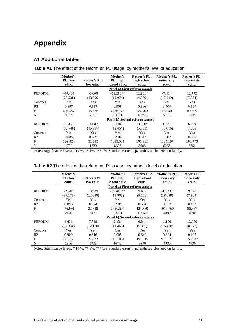
IFAU – The effect of own and spousal parental leave on earnings 41
Appendix
A1 Additional tables
Table A1 The effect of the reform on PL usage, by mother’s level of education
Mother’s PL: low
educ. Father’s PL:
low educ.
Mother’s PL: high
school educ.
Father’s PL: high school
educ.
Mother’s PL: university
educ.
Father’s PL: university
educ. REFORM
Panel a) First reform sample -40.484 -6.606 -31.210** 12.231* -7.434 12.772
(29.238) (13.599) (12.074) (4.930) (17.149) (7.954) Controls Yes Yes Yes Yes Yes Yes R2 0.897 0.557 0.908 0.596 0.904 0.627 F 408.557 15.586 2386.775 126.709 1081.300 89.595 N 2114 2114 10754 10754 5146 5146 REFORM
Panel b) Second reform sample -2.458 -4.087 2.506 13.550* 1.821 6.070
(30.748) (15.297) (12.454) (5.301) (13.616) (7.256) Controls Yes Yes Yes Yes Yes Yes R2 0.885 0.609 0.904 0.643 0.902 0.686 F 292.824 21.625 1822.531 165.912 1289.197 182.773 N 1730 1730 8606 8606 6266 6266 Notes: Significance levels: * 10 %, ** 5%, *** 1%. Standard errors in parentheses, clustered on family.
Table A2 The effect of the reform on PL usage, by father’s level of education
Mother’s PL: low
educ. Father’s PL:
low educ.
Mother’s PL: high
school educ.
Father’s PL: high school
educ.
Mother’s PL: university
educ.
Father’s PL: university
educ. REFORM
Panel a) First reform sample -2.510 13.989 -35.413** 9.492 -16.395 9.721
(27.176) (12.088) (11.905) (5.106) (18.059) (7.803) Controls Yes Yes Yes Yes Yes Yes R2 0.896 0.574 0.909 0.594 0.903 0.632 F 476.991 22.888 2390.505 121.930 1016.760 86.887 N 2470 2470 10654 10654 4890 4890 REFORM
Panel b) Second reform sample 4.451 7.799 2.431 6.844 1.156 12.650
(27.334) (12.110) (11.468) (5.389) (16.488) (8.178) Controls Yes Yes Yes Yes Yes Yes R2 0.900 0.616 0.905 0.642 0.894 0.695 F 371.289 27.823 2122.051 191.315 911.531 151.987 N 1826 1826 9846 9846 4930 4930 Notes: Significance levels: * 10 %, ** 5%, *** 1%. Standard errors in parentheses, clustered on family.

42 IFAU – The effect of own and spousal parental leave on earnings
Table A3 Robustness, mothers
Prob(earnings>0) LnE given earnings>0 FE DDD FE DDD Mother's PL
Panel a) First reform sample -0.003* -0.017***
(0.001) (0.005) Father's PL 0.004 0.024 (0.003) (0.014) REFORM [0.004] 0.016 [0.022] -0.031 [0.002] (0.022) [0.009] (0.096) Controls Yes Yes Yes Yes R2 0.609 0.609 0.677 0.677 F 21.544 19.976 45.538 41.773 N 18014 18014 16306 16306 Mother's PL
Panel b) Second reform sample -0.001 -0.011*
(0.001) (0.005) Father's PL -0.002 0.061*** (0.003) (0.011) REFORM [-0.001] 0.007 [0.018] 0.032 [0.001] (0.021) [0.010] (0.092) Controls Yes Yes Yes Yes R2 0.639 0.640 0.689 0.684 F 18.358 16.724 46.653 39.258 N 16602 16602 15239 15239 Notes: Significance levels: * 10 %, ** 5%, *** 1%. Standard errors in parentheses, clustered on family.
Table A4 Robustness, fathers
Prob(earnings>0) LnE given earnings>0 FE DDD FE DDD Mother's PL
Panel a) First reform sample 0.000 -0.001
(0.001) (0.003) Father's PL -0.004 -0.028** (0.002) (0.009) REFORM [-0.002] -0.023 [-0.009] 0.074 [0.001] (0.019) [0.006] (0.065) Controls Yes Yes Yes Yes R2 0.658 0.659 0.769 0.769 F 1.691 2.227 72.935 68.220 N 18014 18014 16530 16530 Mother's PL
Panel b) Second reform sample 0.001 -0.004
(0.001) (0.003) Father's PL -0.003 -0.045*** (0.002) (0.008) REFORM [-0.001] -0.005 [-0.014] -0.021 [0.001] (0.017) [0.007] (0.061) Controls Yes Yes Yes Yes R2 0.676 0.675 0.748 0.746 F 1.199 0.770 41.415 35.490 N 16602 16602 15570 15570 Notes: Significance levels: * 10 %, ** 5%, *** 1%. Standard errors in parentheses, clustered on family.

IFAU – The effect of own and spousal parental leave on earnings 43
A2 The timing of variable collection Figure A1 shows the timing of variable collection. All variables are collected at two
points in time: one year before the birth of the child (for notational convenience this is
called t=0 although it in practice means t=-1) and also at child age four (t=4). However,
as is clear from the picture, this is average child ages. Since the variables are measured
the 31st of December each year, this will mean that children born in January will on av-
erage be one month younger than children born in December when the variables are
collected.
The parental leave variables are measured as the cumulative amount of parental leave
up to child age three. The motivation is that it is not very interesting to estimate the di-
rect effect of parental leave today on earnings today. Rather, the interesting relationship
is that between early parental leave on future earnings.
1994
A: yob=1994 (Dec)
B: yob=1995 (Jan)
Controls collected in Dec 1993 for A & B (t=0)
Dependent variables measured in Dec 1998 for A & B (t=4)
1993 1995 1996 1997 1998 Special case: PL is measured up to Dec 1997 for A & B
Figure A1 The timing of variable collection: example for reform cohort, first reform sample

44 IFAU – The effect of own and spousal parental leave on earnings
A3 Details of the parental leave benefits over the years
Period SGI days
% of income
reimbursed
"Roof" of yearly income (SEK)
Max SEK/day, SGI days
Max SEK day
if SGI=0 Flat rate
days
SEK/dat, flat rate
days 1990 360 90 222750 549 60 90 60 1991 360 90 241500 595 60 90 60 1992 360 90 252750 623 60 90 60 1993 360 90 258000 636 60 90 60 1994a 360 90 264000 651 64 90/0 60/0 1995b 360 80 267750 587 60 90 60 1996c 360 75 271500 558 60 90 60 1997 360 75 272250 559 60 90 60 1998 360 80 273000 598 60 90 60 1999 360 80 273000 598 60 90 60 2000 360 80 274500 602 60 90 60 2001 360 80 276750 607 60 90 60 2002d 390 80 284250 623 120 90 60 2003 390 80 289500 635 150 90 60 2004 390 80 294750 646 180 90 60 2005 390 80 295500 648 180 90 60 2006 (to June 30) 390 80 297750 653 180 90 60 2006 (from July 1) 390 80 397000 870 180 90 180 2007 390 80 398567 874 180 90 180 2008 390 80 397700 872 180 90 180 2009 390 80 415160 910 180 90 180 Notes: a) During the second half of 1994, the flat rate days were temporarily abolished for children >1 year old. b) The first "daddy month" was introduced for children born after the 1st of january, 1995. During the 30 days set aside for each parent (the daddy month), the reimbursement level for the SGI days was still 90% of previous income. c) During the 30 days set aside for each parent (the daddy month), the reimbursement level for the SGI days was still 85% of previous income. d) The second "daddy month" was introduced for children born after the 1st of january, 2002.

Publication series published by the Institute for Labour Market Policy Evaluation (IFAU) – latest issues
Rapporter/Reports
2009:20 Böhlmark Anders, Oskar Nordström Skans and Olof Åslund ”Invandringsålderns betydelse för social och ekonomisk integration”
2009:21 Sibbmark Kristina ”Arbetsmarknadspolitisk översikt 2008”
2009:22 Eliason Marcus ”Inkomster efter en jobbförlust: betydelsen av familjen och trygghets–systemet”
2009:23 Bennmarker Helge, Erik Grönqvist and Björn Öckert ”Betalt efter resultat: utvärdering av försöksverksamhet med privata arbetsförmedlingar”
2009:24 Hensvik Lena, Oskar Nordström Skans and Olof Åslund ”Sådan chef, sådan anställd? – Rekryteringsmönster hos invandrade och infödda chefer”
2010:1 Hägglund Pathric ”Rehabiliteringskedjans effekter på sjukskrivningstiderna”
2010:2 Liljeberg Linus and Martin Lundin ”Jobbnätet ger jobb: effekter av intensifierade arbetsförmedlingsinsatser för att bryta långtidsarbetslöshet”
2010:3 Martinson Sara ”Vad var det som gick snett? En analys av lärlingsplatser för ung-domar”
2010:4 Nordström Skans Oskar och Olof Åslund ”Etnisk segregation i storstäderna – bostadsområden, arbetsplatser, skolor och familjebildning 1985–2006”
2010:5 Johansson Elly-Ann ”Effekten av delad föräldraledighet på kvinnors löner”
Working papers
2009:21 Åslund Olof, Anders Böhlmark and Oskar Nordström Skans “Age at migration and social integration”
2009:22 Arni Patrick, Rafael Lalive and Jan C. van Ours ”How effective are unemployment benefit sanctions? Looking beyond unemployment exit”
2009:23 Bennmarker Helge, Erik Grönqvist and Björn Öckert “Effects of outsourcing employ–ment services: evidence from a randomized experiment”
2009:24 Åslund Olof, Lena Hensvik and Oskar Nordström Skans “Seeking similarity: how immigrants and natives manage at the labor market”
2009:25 Karlsson Maria, Eva Cantoni and Xavier de Luna “Local polynomial regression with truncated or censored response”
2009:26 Caliendo Marco “Income support systems, labor market policies and labor supply: the German experience”
2009:27 Brewer Mike “How do income-support systems in the UK affect labour force participation?”
2009:28 Gautier Pieter A. and Bas van der Klaauw “Institutions and labor market outcomes in the Netherlands”
2009:29 Brugiavini Agar “Welfare reforms and labour supply in Italy”

2009:30 Forslund Anders “Labour supply incentives, income support systems and taxes in Sweden”
2009:31 Võrk Andres “Labour supply incentives and income support systems in Estonia”
2009:32 Forslund Anders and Peter Fredriksson “Income support systems, labour supply incentives and employment – some cross-country evidence”
2010:1 Ferraci Marc, Grégory Jolivet and Gerard J. van den Berg “Treatment evaluation in the case of interactions within markets”
2010:2 de Luna Xavier, Anders Stenberg and Olle Westerlund “Can adult education delay retirement from the labour market?”
2010:3 Olsson Martin and Peter Skogman Thoursie “Insured by the partner?”
2010:4 Johansson Elly-Ann “The effect of own and spousal parental leave on earnings”
Dissertation series
2009:1 Lindahl Erica “Empirical studies of public policies within the primary school and the sickness insurance”
2009:2 Grönqvist Hans “Essays in labor and demographic economics”
2009:3 Vikström Johan “Incentives and norms in social insurance: applications, indentifications and inference”
2009:4 Nilsson Peter “Essays on social interactions and the long-term effects of early-life conditions”


