The Effect of R&D investments on Economic Inequality Sung Tai Kim * ⋅ Byung In Lim ** , Myung–kyu Kim ** In this paper, we examine the effects of R&D investments on economic inequality in Korea using a dynamic Computable General Equilibrium model. In the model we classify household sector into 10 income groups and classify production sector into 28 industries. Policy simulation is designed to investigate the effect of R&D investments in 28 industries on income distribution during 2008-30 period based on assumption that the R&D investments follow the recent trend. Findings of policy simulation are as follows. Firstly, the R&D investments aggravate the income distribution, while they significantly improve the most major economic variables such as GDP, investments, consumptions during 2008-30 periods. Thus, there exists a trade-off between efficiency and equity aspects of R&D. We try to explain the reason why R&D investments aggravate the income distribution and find that aggravation of income distribution comes from that of capital income distribution relative to labor income distribution. Secondly, we examine the welfare effect of R&D investments based on the equivalent variation. As expected R&D investments increase the welfare of upper income classes relative to income classes. We figure out that the upper income classes consume more R&D intensive goods than the lower income classes and furthermore the prices of R&D intensive goods will probably decrease more due to R&D investments. JEL Classification: L6, H2 Keywords: R&D Investments, Economic Inequality, Income Distribution, Equivalent Variation, Dynamic CGE Model * Professor , Department of Economics, Cheongju University, e-mail: [email protected]** Associate Professor, Department of Economics, Chungbuk University, e-mail: [email protected]** Researcher, Chungbuk Rearch Institute, e-mail: [email protected]
Transcript
The Effect of R&D investments on Economic Inequality
Sung Tai Kim* ⋅ Byung In Lim**, Myung–kyu Kim**
In this paper, we examine the effects of R&D investments on economic inequality in Korea using a dynamic Computable General Equilibrium model. In the model we classify household sector into 10 income groups and classify production sector into 28 industries. Policy simulation is designed to investigate the effect of R&D investments in 28 industries on income distribution during 2008-30 period based on assumption that the R&D investments follow the recent trend.
Findings of policy simulation are as follows. Firstly, the R&D investments aggravate the income distribution, while they significantly improve the most major economic variables such as GDP, investments, consumptions during 2008-30 periods. Thus, there exists a trade-off between efficiency and equity aspects of R&D. We try to explain the reason why R&D investments aggravate the income distribution and find that aggravation of income distribution comes from that of capital income distribution relative to labor income distribution.
Secondly, we examine the welfare effect of R&D investments based on the equivalent variation. As expected R&D investments increase the welfare of upper income classes relative to income classes. We figure out that the upper income classes consume more R&D intensive goods than the lower income classes and furthermore the prices of R&D intensive goods will probably decrease more due to R&D investments. JEL Classification: L6, H2 Keywords: R&D Investments, Economic Inequality, Income
Distribution, Equivalent Variation, Dynamic CGE Model
* Professor , Department of Economics, Cheongju University, e-mail: [email protected]
** Associate Professor, Department of Economics, Chungbuk University, e-mail: [email protected]
In 21st Century, the socioeconomic environments are changing very rapidly. Globalization and aging have been main theme of most countries including Korea and the paradigm of the world economy also has been changing. Especially the knowledge capital and the human capital will play more important role in comparison with the physical capital. Korea will be in the trap of low potential economic growth without new economic growth strategy focusing the total productivity of the economy as a whole.
It is necessary for us to develop the science and technology innovation and accumulate the knowledge capital and the human capital. In order to achieve our purpose we must increase R&D investments and the efficiency of the R&D investments. An increase in R&D investments is expected to increase GDP through various channels in the economy. The R&D investments will increase the knowledge capital stock, which then increases total factor productivity. An increase in total factor productivity will increase the GDP. The R&D investments may have labor saving technical progress and/or capital saving technical progress. In either way an increase in R&D will induces cost saving in production process, which eventually affect GDP positively.
The R&D investments, however, may have negative effect on the distribution of income and economic welfare. Most, if not all, R&D investments are put in the high-tech industry such as information, biology, communication, and environment industries. Those industries are featured to be very R&D intensive, since the technology innovations in those industries require high level of scientific and technical man power and equipments, implying high level of R&D investments as a whole. One of crucial economic achievements of R&D investments is to lower the price of consumer goods, which eventually increase the welfare of households. In that process the upper income class households may enjoy lowered prices of R&D intensive goods in comparison with the lower income class households. As a result, the R&D investments may aggravate the welfare distribution.
The purpose of the study is to analyze the economic effects of R&D investments of 28 industries in Korea more scientifically and systematically. We use the dynamic Computable General Equilibrium (hereafter, CGE) Model to analyze the economic effects of the industrial R&D investments for
2
28 industries in terms of both efficiency and equity aspects. The policy simulation analysis of R&D investments may be classified into two sorts, partial equilibrium analysis and general equilibrium analysis. Recently the general equilibrium approach has been used more often than before due to very rapid development of computation devices and software. To examine the effect of large policy changes as well as to consider many more industry sectors and consumers, Shoven and Whalley (1972) suggest a computable general equilibrium model. The computable general equilibrium model is very powerful in examining both efficiency and equity effects of various policy proposals. Thus, in this paper we use the dynamic Computable General Equilibrium (CGE) model to examine the effects of R&D investments on the macroeconomic variables as well as income distribution of the Korean economy.
The contents of this study are as follows. In the first chapter, we explain the motivation and the background of the research as well as the purpose of the research. In chapter Ⅱ, we survey the literature o
and the Computable General Equilibrium Model. Then we postulate the dynamic CGE model for Korea based on the variety of data. In chapter Ⅲ we examine the effects of R&D investments of 28 industries assuming that the recent trends of R&D investments for each industry will persist in the future for 2008-2030 period. We examine the effect of R&D investments on income distribution and the distribution of economic welfares as well as macroeconomic variables. In chapter Ⅳ we conclude the study and suggest policy implications based on the results of this study.
II. DYNAMIC CGE MODEL
2.1 Literature Survey
There are many works on dynamic CGE Model, such as Fullerton et al.(1983), Ballard et al(1985), Auerbach and Kotlikoff (1987), Fullerton and Rogers(1993), to name a few.
3
On the other hand, there are also many works on the relationship between R&D and the income distribution like Garcia-Penalosa and Turnovsky (2006), Chou and Talmain (1996), Li (1998), Zweimuller (2000), and Foellmi and Zweimuller (2006). However, these especially handles the effects of wealth inequality on the growth. Also, Bertola et al., (chapter 10, 2006) studies the distribution of income between entrepreneurs and workers.
Now we discuss the following works: Berman-Bound-Griliches (1994), Aghion (2002), Grossmann (2007), Chu (2010), Latzer (2011).
Berman-Bound-Griliches (1994) found that R&D expenditure and computer purchase could explain as much as 70% of the move away from production to non-production labor over the period 1979-1987.
Aghion (2002) tried to explain why within-group wage inequality has been increased sharply during the past thirty years in developed countries like US and UK and found that it results partly from a innovation response to the increased supply of skilled labor. He used Schumpeterian Growth theory which offers a suitable framework for a more general analysis of the relationship growth and income inequality. His study implies that between- versus within-group wage inequality implies labor market policy during the transition to a new technological paradigm.
Grossmann (2006) compared the positive and normative implications of two alternative measures to promote R&D-based growth with an overlapping generation model. R&D subsidies to firms may be harmful to both productivity growth and welfare, and furthermore earnings inequality (p. 13). On the while, publicly provided education targeted to science and engineering skills promotes growth unambiguously and is neutral for the earnings distributions. Importantly, this holds true although intertemporal knowledge spillovers are the only externality from R&D spending of firms in the model. The main reason is a congestion effect under a public education system, implying that the public education is a rival good and R&D activity requires human resources with specialized skills. Earning inequality is divided into two classifications: earnings inequality within the group of R&D workers and between R&D labor abd production workers. Earnings inequality within the group of R&D workers is calculated form the top to bottom earners within this group, but between-group inequality is measured from the ratio of average income between two groups, i.e., R&D labor abd production workers. As a result, this study shows that a more desirable
4
means to promote R&D is to increase public expenditure targeted to the education of scientists and engineers.
Chu (2009) develops a quality-ladder growth model with wealth heterogeneity and elastic labor supply and claimed that strengthening patent protection increases both economic growth and income inequality. The increase in income inequality results from raising the return on assets. However, whether it increases consumption inequality depends on the elasticity of intertemporal substitution. He showed that strengthening patent protection worsens income inequality by more than consumption inequality, using the US data. If the elasticity of intertemporal substitution is less (greater) than unity, strengthening patent protection would increase(decrease) consumption inequality. He found that patent policy may explain the recent trend of income and consumption inequality in the US partly. The logic ia as follows: strengthening patent protection increases R&D and thus drives up the rate of return on assets. It increases the income of asset-wealthy households more than the asset-poor households. Also the higher growth rate increases the fraction of assets that needs to be saved. Therefore, whether the relative increase between the asset-wealthy households and asset-poor households increases or decreases depends on the elasticity of intertemporal substitution.
Latzer (2011) showed that inequality have an impact on the allocation of the overall R&D effort between incumbents and challengers with a Schunpetrian model of growth and inequality. He also claimed that a higher level of inequalities leads to a bigger share of the overall R&D investment to be carried out by quality leaders. 2.2 Model Overview
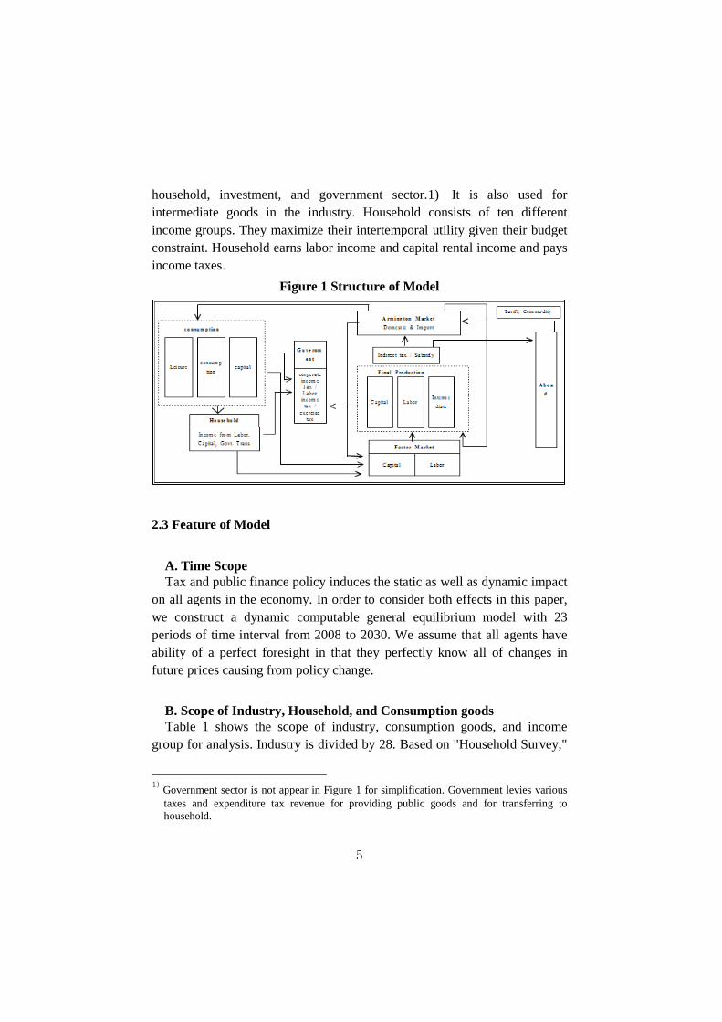
Figure 1 shows a brief structure of the model developed in this paper.
Employing labor and capital, firm produces a final goods (Yi) and sell it to both domestic and abroad. In this process, government levies an indirect tax or a subsidy on the final goods. As shown in the figure, after paying tariff and/or commodity tax, imported goods flows into Armington market where imported goods is treated as imperfect substitute for domestic counterparts. The compounded consumption goods at Armington market is distributed to
5
household, investment, and government sector.1) It is also used for intermediate goods in the industry. Household consists of ten different income groups. They maximize their intertemporal utility given their budget constraint. Household earns labor income and capital rental income and pays income taxes.
Figure 1 Structure of Model
2.3 Feature of Model
A. Time Scope Tax and public finance policy induces the static as well as dynamic impact
on all agents in the economy. In order to consider both effects in this paper, we construct a dynamic computable general equilibrium model with 23 periods of time interval from 2008 to 2030. We assume that all agents have ability of a perfect foresight in that they perfectly know all of changes in future prices causing from policy change.
B. Scope of Industry, Household, and Consumption goods Table 1 shows the scope of industry, consumption goods, and income
group for analysis. Industry is divided by 28. Based on "Household Survey,"
1) Government sector is not appear in Figure 1 for simplification. Government levies various
taxes and expenditure tax revenue for providing public goods and for transferring to household.
6
we consider 10 income groups who a representative household spends its income on 10 different consumption goods. Therefore, the model is designed to analyze both equity and efficiency issues causing from policy change.
Table 1 Scope of Industry, Consumption, and Income Group Industry Consumption Income Group
S01 Agricultural and marine Products S15 Transport equipment C01 Food products
and beverages W01. 0~10%
S02 Mineral products S16 Furniture and manufacturing products
C02 Housing expense W02.10~20%
S03 Food products and beverages
S17 Electric power, gas and water service
C03 Light, heat and water services W03. 20~30%
S04 Textile and leather products S18 Construction C04 Furniture and
appliances W04. 30~40%
S05 Wood and paper products
S19 Wholesale and retail trade
C05 Clothing and footwear W05. 40~50%
S06 Printing, publishing and reproduction
S20 Restaurant and accommodation
C06 Health and medical services W06. 50~60%
S07 Petroleum and coal products S21 Transport and storage C07 Education W07. 60~70%
S08 Chemical products S22 Telecommunications and broadcasting
C08 Cultural recreation W08. 70~80%
S09 Non-metallic mineral products S23 Financial and insurance C09 Traffic and
communication W09. 80~90%
S10 Basic metal products S24 Real estate and Business activities C10 Others W10. 90~100%
S11 Metal products S25 Public administration and national defense
S12 General machinery S26 Education and health S13Electrical and electronic
instruments S27 Social and other
services
S14 Precision instruments S28 Others
2.4 Model Structure A. Household Household consists of 10 income groups. It is assumed that each income
group has a representative agent who lives infinitively and is able to foresee perfectly. Each consumer maximizes his intertemporal utility function (Uw) subject to an intertemporal budget constraint. It is also assumed that intertemporal utility function is CES (constant elasticity of substitution) between full consumption (Zw,t) at any points in time t .
7
1,
, 0max ( )
1w tt
w w tL t
ZU Z
θ
aβ
θ
−∞
== ∑
− (1)
1
, , , ,. . [ (1 )( ) ]w t w t w t w ts t Z Q H Lρ ρ ρa a= + − − (2)
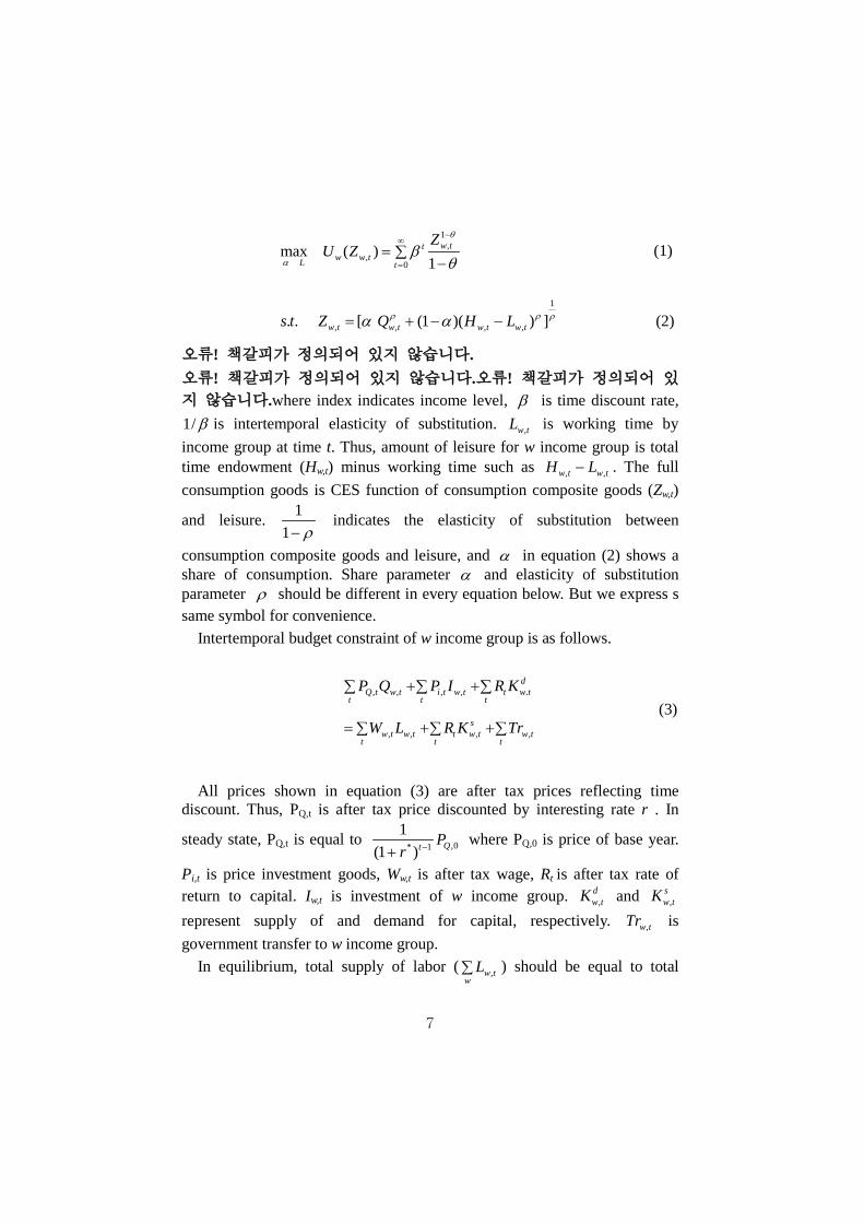
오류! 책갈피가 정의되어 있지 않습니다. 오류! 책갈피가 정의되어 있지 않습니다.오류! 책갈피가 정의되어 있지 않습니다.where index indicates income level, β is time discount rate, 1/ β is intertemporal elasticity of substitution. ,w tL is working time by income group at time t. Thus, amount of leisure for w income group is total time endowment (Hw,t) minus working time such as , ,w t w tH L− . The full consumption goods is CES function of consumption composite goods (Zw,t)
and leisure. 11 ρ−
indicates the elasticity of substitution between
consumption composite goods and leisure, and a in equation (2) shows a share of consumption. Share parameter a and elasticity of substitution parameter ρ should be different in every equation below. But we express s same symbol for convenience.
Intertemporal budget constraint of w income group is as follows.
, , , , .
, , , ,
dQ t w t i t w t t w t
t t t
sw t w t t w t w t
t t t
P Q P I R K
W L R K Tr
+ +∑ ∑ ∑
= + +∑ ∑ ∑ (3)
All prices shown in equation (3) are after tax prices reflecting time
discount. Thus, PQ,t is after tax price discounted by interesting rate r . In
steady state, PQ,t is equal to ,0* 1
1(1 ) Qt P
r −+ where PQ,0 is price of base year.
Pi,t is price investment goods, Ww,t is after tax wage, Rt is after tax rate of return to capital. Iw,t is investment of w income group. ,
dw tK and ,
sw tK
represent supply of and demand for capital, respectively. ,w tTr is government transfer to w income group.
In equilibrium, total supply of labor ( ,w tw
L∑ ) should be equal to total
8
demand for labor ( ,i ti
L∑ ), and also total supply( ,sw t
wK∑ ) of capital should be
equal to total demand for capital ( ,i ti
K∑ + ,dw t
wK∑ ) .
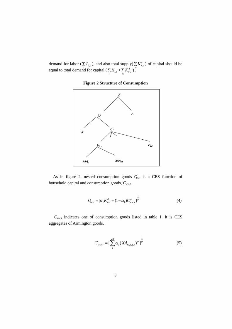
Figure 2 Structure of Consumption
As in figure 2, nested consumption goods Qw,t is a CES function of
household capital and consumption goods, Cw,c,t.
1
, 1 , 1 , ,[ (1 ) ]dw t w t w c tQ K C ρ ρa a= + − (4)
Cw,c,t indicates one of consumption goods listed in table 1. It is CES
aggregates of Armington goods.
∑=28 1
,,,,, ])([i
ticwitcw XAC ρρa
(5)
9
Where , , ,w c i tXA is i Armington goods for producing c consumption goods for w income group at time t.
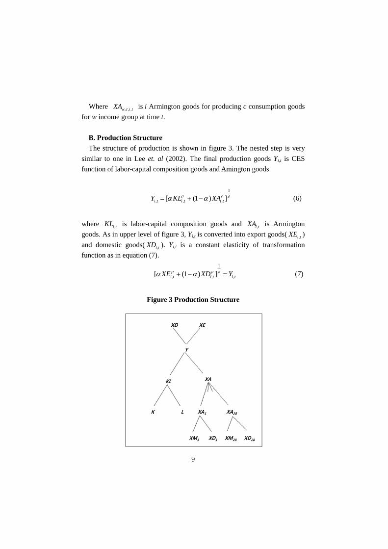
B. Production Structure The structure of production is shown in figure 3. The nested step is very
similar to one in Lee et. al (2002). The final production goods Yi,t is CES function of labor-capital composition goods and Amington goods.
1
, , ,[ (1 ) ]i t i t i tY KL XAρ ρ ρa a= + − (6)
where ,i tKL is labor-capital composition goods and ,i tXA is Armington goods. As in upper level of figure 3, Yi,t is converted into export goods( ,i tXE ) and domestic goods( ,i tXD ). Yi,t is a constant elasticity of transformation function as in equation (7).
1
, , ,[ (1 ) ]i t i t i tXE XD Yρ ρ ρa a+ − = (7)
Figure 3 Production Structure
10
In equation (6), labor and capital composite goods is CES function of labor
and capital.
1
, , ,[ (1 ) ]i t i t i tKL L Kρ ρ ρa a= + − (8)
Li,t indicates a labor input and Ki,t is a capital used in sector i. In equation (6), Armington goods is CES function of domestic
goods( ,s tXD ) and imported goods( ,s tXM ) as shown in equation (9). We use index s instead of i to distinguish Armington goods used in industry and household, government, and investment sectors.
1
, , ,[ (1 ) ]s t s t s tXA XD XMρ ρ ρa a= + − (9)
,s tXA stand for 28 production goods in table 1. Armington goods is distributed to i industry as intermediary goods and to household, government, and investment sector as final consumption goods.
, , , , , , , , , ,s t s i t w c s t inv s t g s ti w c
XA XA XA XA XA= + + +∑ ∑∑ (10)
where , ,s i tXA is s Armington goods used in i industry as intermediary goods.
, , ,w c s tXA is s Armington goods consumed by w income group, , ,inv s tXA is one used by investment sector, and , ,g s tXA is one used in government sector.
C. Factor Market i) Labor Market Aggregate labor input consists of labors supplied by each income group.
11
Individual labor input differs only in terms of amount of tax burden because of the graduation of labor tax in Korea. Compounded each individual labor input at the labor market, aggregated labor is distributed into each industry. Equation (11) shows the process of compounding an individual labor input. Equation (12) shows distribution of a compounded labor into i industry. As shown in equation (12), labor input is CES aggregation of individual labor.
( )1
,t w w tw
L L ρρa= ∑ (11)
,t i ti
L L= ∑ (12)
ii) Capital Market As in labor market, capital market aggregates individual capital with
imperfect substitution as in equation (13), and distributes it into each industry and household.
( )1
,t w w tw
K K ρa= ∑ (13)
, ,d
t i t w ti w
K K K= +∑ ∑ (14)
Where Kt is total capital stock, Kw,t is individual capital stock supplied by
w income group. Ki,t is capital stock used in i industry, and dtwK , is capital
stock demanded by w income group. Unlike in Fullerton and Rogers(1993) and Lee et al(2002), our model is
fully dynamic model which is solved all period simultaneously. Each period is connected by accumulation of capital stock. Capital stock of t + 1 period is accumulated by following law of motion.
1 ,(1 )t i t tK K Iδ+ = − + (15)
where δ is depreciation rate and It is investment at period t .
12
D. Government Government collects tax and spends it on consuming and transferring to
household.
, 1, , 2, ,
3, 4, , , , 5, 6, , , , ( ) ( )
t ex t t i t i t i t i ti i
i i em i t i t i i i t i ti i
P D r K w L
P XM P Ym
t t
t t t t
Φ + = +∑ ∑
+ + + +∑ ∑ (16)
where tΦ is government total tax revenue and Dg,t is government deficit
that is defined as total its revenue minus total expenditure. ,ex tP is exchange rate. We use exchange rate as price of government deficit because of allowing for government to finance its deficit from abroad. 1,it is an effective tax rate on corporate income, 2,it is an average tax rate on labor income, 3,it is tariff rate, and 4,it is imported commodity tax rate. 5,it is indirect tax rate, and 6,it is subsidy rate. , ,u i tP is price of i goods before tax. rt and wt are wage and rate of returns to capital before tax. , ,xm i tP is before tax price of imported goods.
On the other hand, government expenditure ( tΓ ) is defined as follow.
, , ,st XA t s t w ts w
P XA TrΓ = +∑ ∑ (17)
where ,sXA tP is before tax price of s Amington goods (XAs,t) and Trw,t is
government transfer to w income group. We can consider two kinds of budget constraints. One is period by period
balancing government budget. The other one is balancing government budget over infinite period.
,t ex t t tP DΦ + = Γ (18)
,0 0 0
t ex t t tt t t
P D= = =Φ + = Γ∑ ∑ ∑ (19)
13
We calibrate government budget to balance without levying endogenous tax in base year. After new policy is induced, however, government budget preserves the balance through adjusting consumption tax rate endogenously. Consumption tax is endogenously changed every period in period by period budget balancing constraint, while only one consumption tax rate is endogenously determined in balancing over whole period.
E. International Trade Assuming small open economy, we consider the price of imported goods
as exogenously given variable. However, imbalance of trade is settled through capital flow from abroad or through changing in exchange rate. Under perfect capital market, we can define trade balance constraint as equation (20).
, , , , 0XEt t i t XMt t i t ex ti i
P XE P XM P B− + =∑ ∑ (20)
where ,XEt tP and ,XMt tP are after tax prices of export and imported goods respectively. exP is exchange rate fixed over time. Therefore, changing in Bt preserves trade balance.
The other way to preserve trade balance is to assume that exports equal imports in each period. Under this balance of payments constraint, capital flows are restricted and the domestic interest rate is therefore endogenous.
, , , , , 0 0XEt t i t XMt t i t ex ti i
P XE P XM P B− + =∑ ∑ (21)
Unlike equation (20), trade imbalance (B0) is fixed over time but exchange
rate ,ex tP is endogenous, instead.
14
2.5 Input Data
The base year is 2008 year in this paper. The input data for this model come from various sources; 2008 Input-Output Tables, Household Survey, Statistical Yearbook of National Tax, Financial Statement Analysis, Korea Statistical Yearbook, and previous studies. Since Survey for Household Survey and Financial Statement Analysis 2008 are based on survey, we need to consistently connect to aggregate macro-data. In order to do that, we calculate the ratio of consumption, investment, income, etc, first. Applying these ratios to macro data, we construct micro & macro-consistent data set which are components of SAM (Social Account Matrix) in table 2.
Table 2 shows the economic transaction of Korea, 2008. A SAM is a comprehensive, economy-wide data framework, typically representing the all transaction of s economy. More technically, a SAM is a square matrix in which each account is represented by a row and a column. Each cell shows the payment from the account of its column to the account of its row - the incomes of an account appear along its row, its expenditures along its column. The dimension in table 2 represents the sub-transaction of each account.
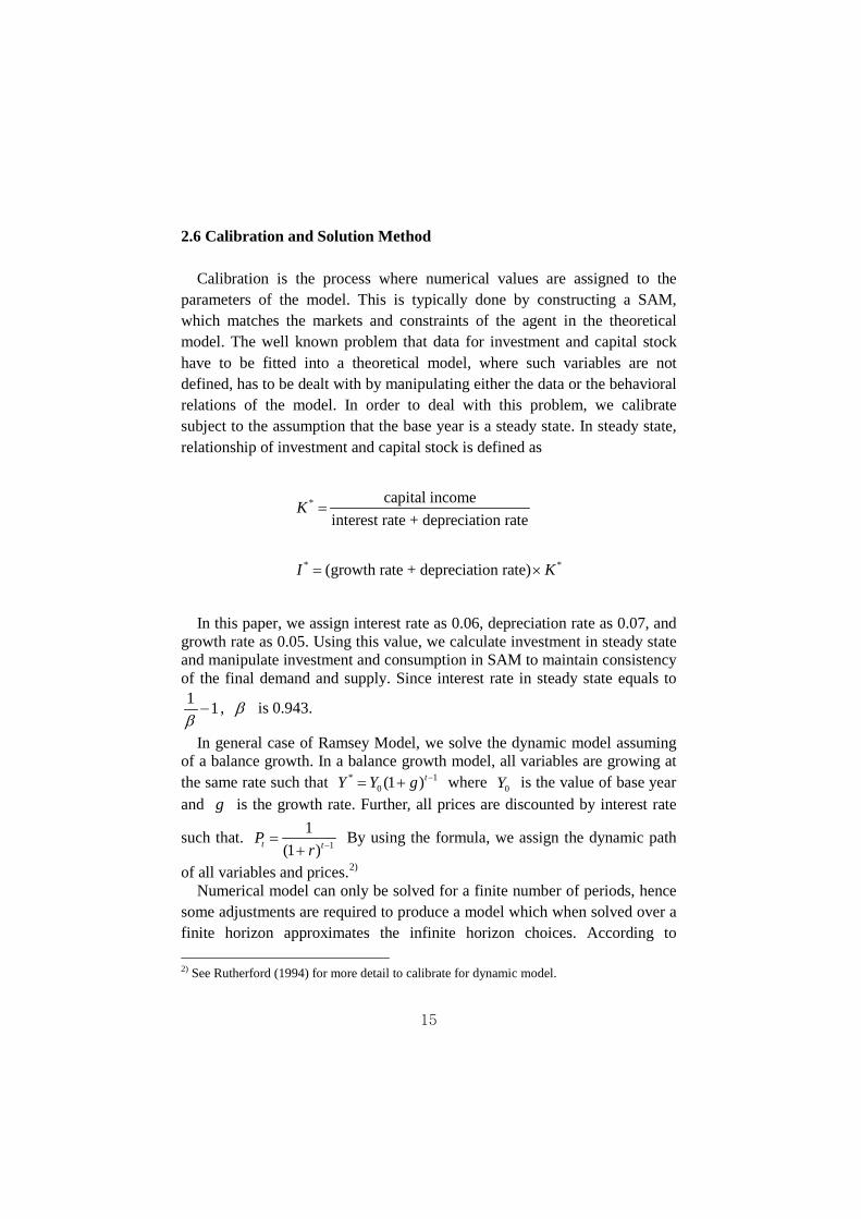
Calibration is the process where numerical values are assigned to the parameters of the model. This is typically done by constructing a SAM, which matches the markets and constraints of the agent in the theoretical model. The well known problem that data for investment and capital stock have to be fitted into a theoretical model, where such variables are not defined, has to be dealt with by manipulating either the data or the behavioral relations of the model. In order to deal with this problem, we calibrate subject to the assumption that the base year is a steady state. In steady state, relationship of investment and capital stock is defined as
*
* *
capital incomeinterest rate + depreciation rate
(growth rate + depreciation rate)
K
I K
=
= ×
In this paper, we assign interest rate as 0.06, depreciation rate as 0.07, and
growth rate as 0.05. Using this value, we calculate investment in steady state and manipulate investment and consumption in SAM to maintain consistency of the final demand and supply. Since interest rate in steady state equals to 1 1β− , β is 0.943.
In general case of Ramsey Model, we solve the dynamic model assuming of a balance growth. In a balance growth model, all variables are growing at the same rate such that * 1
0 (1 )tY Y g −= + where 0Y is the value of base year and g is the growth rate. Further, all prices are discounted by interest rate
such that. 1
1(1 )t tP
r −=+
By using the formula, we assign the dynamic path
of all variables and prices.2) Numerical model can only be solved for a finite number of periods, hence
some adjustments are required to produce a model which when solved over a finite horizon approximates the infinite horizon choices. According to 2) See Rutherford (1994) for more detail to calibrate for dynamic model.
16
Rutherford (1994), we add a constraint on the growth rate of investment and GDP in the terminal period such that they are the same.
We choose the other parameters, basing on previous researches: Fullerton and Rogers(1993), Sonn and Shin(1997), Cho(2000), Lee et al.(2002), Bernstein et al.(1999), Goulder and Schneider(1999).
We assume that all sectors have same value of elasticity of substitution. According to Sonn and Shin(1997) who used 2~4, We choose 3.0 of constant elasticity of transformation between exports and domestic goods. The elasticity of substitution between labor and capital is one in which this functions has Cobb-Douglas production technology. Based on Fullerton and Rogers(1993) and Lee et al(2002), We assume that the elasticity of capital-labor compound good and Amington goods is 0. We assign 3.0 to elasticity of Amington transformation with same reason for choosing an elasticity of transformation between exports and domestic goods.
The elasticity of intertemporal substitution (1/θ ) is 0.5 based on Goulder and Schneider (1999) and Bernstein et al(1999). We choose 0.8 of elasticity of compound consumption good and leisure according to Rasmessen and Rutherford (2001).
The model in this paper is programmed in GAMS language. Under the GAMS platform, the dynamic structure of the model is written in MPSGE which is an abstract, high-level language for formulating CGE model. The equilibrium prices and quantities of the model are solved by using the PATH solver, a generic algorithm for solving MCP (Mixed Complementary Programming) problems. The main advantage of programming in MPSGE is that the solution algorithm and the economic model can be separated. This separation makes it possible for users to make changes in model structure, and to introduce new assumptions, without extensive re-programming and debugging.
17
III. The Effect of R&D investments: POLICY SIMULATION
3.1 Policy Simulation Design
In the policy simulation, we try to analyze the economic effects of R&D investments which we assume will follow the recent trends in the future. Based on the assumptions we estimate the R&D investments for 28 industries during the 2008-2030 periods, using the ARIMA (Autoregressive Integrated Moving Average) time series model. In the next stage, we analyze the economic effects of the R&D investments on terms of efficiency and equity aspects. In terms of efficiency aspects, we focus on the effects of R&D investments on the demand side of the economy such as GDP, consumption, investments, government expenditures and net export (which is export minus import). We analyze the effects on the supply side of the economy such as capital formation, labor supply, and real wage.
3.2 The effect of R&D investment on major macro variables
The followings are the main results of the policy simulation. We compare the counter-factual equilibrium with the benchmark equilibrium. The counter-factual equilibrium is one in which the R&D investments will increase following the recent trends for 28 industries. We find that in the counter-factual equilibrium the GDP will increase by 0.60% annually in comparison with the benchmark equilibrium. The consumption will increase by 0.19% annually and the investment will increase by 1.27% annually. In addition the government expenditures will increase 0.44% annually and the trade balance will increase by 9.62% annually.
In terms of the effects on the supply side of the economy, the capital stock will increase by 0.96% annually and the labor supply will increase by 0.32% annually. Therefore, the efficiency gain of the R&D investments will be substantial.
In this study, we estimate the elasticity of GDP with respect to the R&D investment, which is the ratio of the % increase of GDP to the % increase.
18
The estimate of the elasticity of GDP with respect to the R&D investment for 2009 is 0.404 and will increase smoothly to reach 1.037 in 2026. We may confirm that there exists "Increasing Returns To Scale" in R&D investments. Also we may notice that there exists the lagged effect and the cumulative effects of the R&D investments. The lagged effect of R&D means that the effect of R&D in current year will be realized after few years. The cumulative effect of R&D refers to the fact that as time goes by the effect of R&D will exist for quite a long period. 3.3 Income Distribution Effect of R&D
It is desirable to analyze the economic effects of R&D investment in terms of both efficiency and equity aspects. On the one hand, an efficiency analysis on the effect of R&D investment on the size of total pie, for instance, either GDP or social welfare. On the other hand, an equity analysis focuses on the effect of R&D investment on the distribution of total pie among economic agents.
In section 3.2 it was shown that the effect of R&D investment on the major macro economic variables are seemingly marvelous. Here we will analyze the equity aspect of R&D investment in terms of the welfare effect and the income distribution effect. It is more meaningful and fruitful to analyze both, since the two have slightly different implications. the welfare effect of R&D investment is more sensible for analyzing equity aspect of R&D. However, the welfare comparison of any two states is more or less difficult, because factors affecting the welfare of different income class households are often too complex including simultaneous price scheme and income changes. On the other hand, the income distribution effect of R&D investments can be easily analyzed based on change in Gini-coefficient. Also the income variable is a very good proxy variable for welfare.
There is a large number of measures that summarize economic inequality and make comparisons over time within one country and between countries (see Sen(1973) and Jenkins(1991)). The most commonly used measures are quantile shares, distribution ratios, Lorenz curves and associated Gini coefficients. In the case of completely equal distribution of income, G=0, where the Lorenz curve coincides with the 45° line. On the other hand, in
19
the case of completely unequal distribution of income (one unit all the income), G=1.
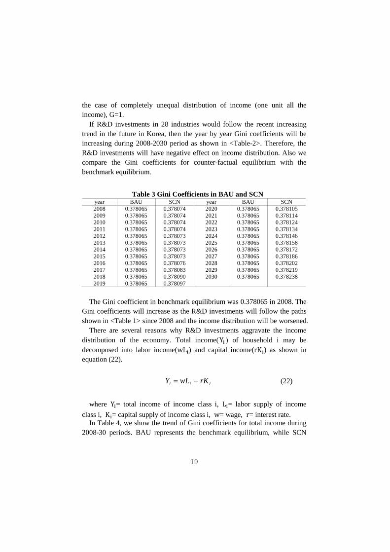
If R&D investments in 28 industries would follow the recent increasing trend in the future in Korea, then the year by year Gini coefficients will be increasing during 2008-2030 period as shown in <Table-2>. Therefore, the R&D investments will have negative effect on income distribution. Also we compare the Gini coefficients for counter-factual equilibrium with the benchmark equilibrium.
The Gini coefficient in benchmark equilibrium was 0.378065 in 2008. The
Gini coefficients will increase as the R&D investments will follow the paths shown in <Table 1> since 2008 and the income distribution will be worsened.
There are several reasons why R&D investments aggravate the income distribution of the economy. Total income(Yi ) of household i may be decomposed into labor income(wLi) and capital income(rKi) as shown in equation (22).
iii rKwLY += (22)
where Yi= total income of income class i, Li= labor supply of income
class i, Ki= capital supply of income class i, w= wage, r= interest rate. In Table 4, we show the trend of Gini coefficients for total income during
2008-30 periods. BAU represents the benchmark equilibrium, while SCN
20
represents the counter-factual equilibrium in which R&D investments are assumed to increase the trend. Also DIF in <Table 3> denotes the difference between the two Gini coefficients for BAU and SCN. Thus, positive DIF implies that Gini coefficient has been increased and aggravated income distribution. We can easily observe that aggravation of total income distribution comes from aggravation of capital income.
Table 4 Decomposition of Total Income Distribution into Labor Income and Capital Income
Note: (1) BAU represents the benchmark equilibrium. (2) SCN represents the counter-factual equilibrium (3) DIF. = SCN - BAU.
3.4 Welfare Distribution Effect of R&D investment
We use equivalent variation as welfare comparison between benchmark equilibrium and counter-factual equilibrium due to R&D investments.
Equivalent variation (EV) is a measure of how much money would pay before a price increase. The value of the equivalent variation is given in terms of the expenditure function ),( ⋅⋅e as
),(),(),(),(
0010
0010
upeupeupeupeEV
−=−=
(23)
where w is the wealth level, 0p and 1p are the old and new prices
respectively, 0u and 1u are the old and new utility levels respectively.
21
Equivalently, in terms of the indirect utility function or the value function ( ),( ⋅⋅v ),
10 )),( uEVwpv =+ (24)
Table 5 Welfare effect of R&D investments in terms of Equivalent Variation
Note : E.V. Difference denotes the difference in equivalent variation between income class i (i = 1, …, 10) and the lowest income class.
The effect of R&D investments on the welfare of 10 income class
households in terms of equivalent variation is shown in Table 5. In Table 5, we provide the difference in equivalent variation between income class i (i = 1, …, 10) and the lowest income class.
We may easily notice that R&D investments aggravate the welfare distribution in terms of equivalent variation. The difference between the income distribution effect and the welfare distribution effect lies in the fact that the latter takes into account price change as well as income change while the latter takes into account only income change due to R&D investments.
We will try to examine why R&D investments aggravate welfare distribution. There are two propositions we want to suggest on why so. First, the upper income class households consume more R&D intensive goods than the lower income class households. Second, the price of more R&D intensive products will decrease more than less R&D intensive products. As a result increase in R&D investments increase welfare of the upper income class
22
households more than the lower income class households, since the upper can enjoy the benefit from lower price of R&D intensive products. These results conforms to the previous studies.
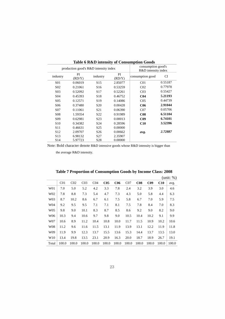
We examine our first proposition by computing R&D intensities of ten consumption goods. In our model there are 28 production goods which are transformed into 10 consumption goods.
where CI denotes 10 consumption good's R&D intensity index, RD/Y denotes the R&D intensity that is defined to be the ratio of R&D investment to output and Z-matrix denotes transition matrix that convert production goods to consumption goods.
In Table 6, index PI denotes the production good R&D intensity and index CI denotes the consumption good R&D intensity. we examine our first proposition by computing R&D intensities of ten consumption goods. In our model there are 28 production goods which are transformed into 10 consumption goods. As expected the electrical and electronic instrument industry (S13) shows the most R&D intensive, and the precision industry (S14), the transport industry (S15), the general machinery industry (S12) follow in order. In terms of consumption good R&D intensity the traffic and communication good (C09) is most R&D intensive, the cultural recreation good (C08) , the furniture and appliance good (C04), and the health and medical services (C06) follow in order.
In Table 7, the proportion of consumption expenditure of income class i relative to whole consumption expenditures, where i=1, ,,, , 10. It turns out that the upper income classes consume more R&D intensive products than the lower income classes.
23
Table 6 R&D intensity of Consumption Goods production good's R&D intensity index consumption good's
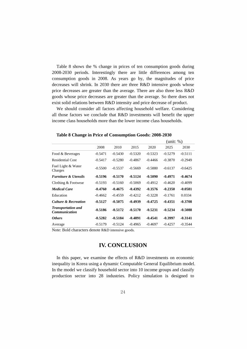
Table 8 shows the % change in prices of ten consumption goods during 2008-2030 periods. Interestingly there are little differences among ten consumption goods in 2008. As years go by, the magnitudes of price decreases will shrink. In 2030 there are three R&D intensive goods whose price decreases are greater than the average. There are also three less R&D goods whose price decreases are greater than the average. So there does not exist solid relations between R&D intensity and price decrease of product.
We should consider all factors affecting household welfare. Considering all those factors we conclude that R&D investments will benefit the upper income class households more than the lower income class households.
Table 8 Change in Price of Consumption Goods: 2008-2030
In this paper, we examine the effects of R&D investments on economic
inequality in Korea using a dynamic Computable General Equilibrium model. In the model we classify household sector into 10 income groups and classify production sector into 28 industries. Policy simulation is designed to
25
investigate the effect of R&D investments in 28 industries on income distribution during 2008-30 period based on assumption that the R&D investments follow the recent trend.
Findings of policy simulation are as follows. Firstly, the R&D investments aggravate the income distribution, while they significantly improve the most major economic variables such as GDP, investments, consumptions during 2008-30 periods. Thus, there exists a trade-off between efficiency and equity aspects of R&D. We try to explain the reason why R&D investments aggravate the income distribution and find that aggravation of income distribution comes from that of capital income distribution relative to labor income distribution.
Secondly, we examine the welfare effect of R&D investments based on the equivalent variation. As expected R&D investments increase the welfare of upper income classes and decrease the welfare of lower income classes. We figure out that the upper income classes consume more R&D intensive goods than the lower income classes and furthermore the prices of R&D intensive goods will decrease more due to R&D investments. Empirically, however, there are mixed relations between R&D intensity and price decrease of consumption good. We should consider all factors affecting household welfare. Considering all those factors we conclude that R&D investments will benefit the upper income class households more than the lower income class households.
REFERENCE
Aghion, P., Schumpeterian Growth Theory and the Dynamics of Income Inequality, Econometrica 70(3), 2002, pp. 855-882.
Auerbach, Alan J. and Laurence J. Kotlikoff, Dynamic Fiscal Policy, Cambridge University Press, 1987.
Ballard, C.D, Fullerton, D., Shoven, J.B. and Whalley J., "A General Equilibrium Model for Tax Policy Evaluation," University of Chicago Press for National Bureau of Economic Research, 1985.
Berman, E., J. Bound and Z. Griliches, Changes in Demand for Skilled Labor Within US Manufacturing: Evidence from the Annual Survey of Manufactures, Quarterly Journal of Economics, 109(2), 1994, pp. 367-97
26
Bernstein, P. M., W. O. Montgomery, and T. F. Rutherford, “Global Impacts of the Kyoto Agreement: Results from MS-MRT Model,” Resource and Energy Economics, 21, 1999, pp. 375-413.
Bertola, G., Foellimi, R. and Zweimuller, J. Income Distribution in Macroeconomic Models, Princeton University Press, 2006.
Cass, D., “Optimum Growth in an Aggregative Model of Capital Accumulation,” Review of Economic Studies, 32, 1965, pp. 233-240.
Cho, Gyeong Lyeob, “The Effect of Green-house Gas Reduction Policy : Global CGE Model Analysis,” (in Korean) Kyong Je Hak Yon Gu, Volume 48 No.4, 2000, pp. 323-368.
Cho, Gyeong Lyeob and I.K. Na, “The Green-house Gas Reduction Policy and Technical Progress,” (in Korean) Kyong Je Hak Yon Gu, Volume 51 No.3, 2003, pp. 263-294.
Chou, C. and Talmain, G, Redistribution and Growth: Pareto Improvements, Journal of Economic Growth, 1, 1996, pp. 505-23.
Chu, A.C., "Effects of Patent Policy on Income and Consumption Inequality in a R&D Growth Model," Southern Economic Journal, 77(2), 2010, pp. 336-350.
Foellmi, R. and Zweimuller, J. Income Distribution and Demand-induced Innovations, Review of Economic Studies, 73, 2006, pp. 941-960.
Fullerton, Don and Diane L. Rogers, Who Bears the Lifetime Tax Burden?, Washington D. C., The Brooking Institution, 1993.
Fullerton, Don, J. B. Shoven and J. Whalley, "Replacing the U.S. Income Tax with a Progressive Consumption Tax: A Sequenced General Equilibrium Approach," Journal of Public Economics 20, 1983, pp. 3~23.
Garcia-Penalosa, C. and Turnovsky, S.J, Growth and Income Inequality: A Canonical Model, Economic Theory, 28, 2006, pp. 25-49.
Goulder, L. H. and Schneider, S. H., “Induced Technological Change and the Attractiveness of CO2 Abatement Policies,” Resource and Energy Economics, 21, 1999, pp. 211-253.
Grossmann, V., "How to promote R&D-based growth? Public education expenditure on scientists and engineers versus R&D subsidies," Journal of Macroeconomics 29(4), 2007, pp. 891-911.
Kim, Sung Tai, “Estimation of Effective Corporate Income Tax Rate By Industry in Korea,” Research Report, 04-4, National Assembly Budget Office, 2004.
Kim, Sung Tai, C.S. Jung, G.L. Cho, S.D. Lee, K.H. Kim, “The Parts and Material Industry Model Analysis,” Research Project by Industry and Resource Department, 2006.
27
Latzer, H., A Schumpeterian Model of Growth and Inequality, working papers of BETA with number 2011-20, 2011.
Li, C.-W, Inequality and Growth: A Schumpeterian Perspective, manuscript, 1998.
Mas-Colell, A., Whinston, M and Green, J., Microeconomic Theory, Oxford University Press, New York, 1995.
Moon, Youngsuk, G.L. Cho, “The Effect of Regulation on Greenhouse gas Emission on the long-run Energy Transformation,” (in Korean) Kyong Je Hak Yon Gu, Volume 53 No.1, 2005, pp. 121-153.
Romer, P. M., “Increasing Returns and Long Run Growth,” Journal of Political Economy, 94(5), 1986, pp. 1002-1037.
Rutherford, T. F., The GAMS/MPSGE and GAMS/MILES User Notes, Washington D.C., GAMS Development Corporation, 1994.
Scarf, H. E., “The Approximation of Fixed Points of a Continuous Mapping,” SIAM Journal of Applied Mathematics, 15(5), 1967, pp. 328-343.
Shoven, J.B. and J. Whalley, “ A General Equilibrium Calculation of the Effects of Differential Taxation of Income from Capital in the U.S.,” Journal of Public Economics, 84, 1976, pp. 281-322.
Shoven, J.B. and J. Whalley, Applying General Equilibrium, Cambridge Surveys of Economic Literature, 1992.
Sonn, Yanghoon and D.C. Shin, “The Effect of Foreign Exchange Rate Variation on Energy Industry,” (in Korean) Kyong Je Hak Yon Gu, Volume 45 No.1, 1997, pp. 123-139.
Yi, Insill, Sung Tai Kim, C.B. Ahn, S.D. Lee, “A Study on the Corporate Income Tax Reform” (in Korean) Research Report 02-12, Korean Economic Research Institute, 2002.
Zweimuller, J., Schumpeterian Entrepreneurs meet Engel's law: The Impact of Inequality on Innovation-driven Growth, Journal of Economic Growth, 5, 2000, pp. 185-206.