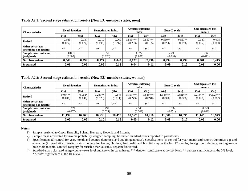
1 THE EFFECT OF RETIREMENT ON MENTAL HEALTH AND SOCIAL INCLUSION OF THE ELDERLY Asenka Asenova Abstract This paper utilises multinational data on 17 countries from the Survey of Health, Ageing and Retirement in Europe to investigate the effect of retirement of the elderly on their psychological well-being and social inclusion. Following the identification strategy used recently by Coe and Zamarro (2011) we use an instrumental variable strategy based on plausibly exogenous variation in retirement probabilities induced by the country-level statutory and early retirement ages. The key findings of the study tell a consistent story: while labour force exit has no significant impact on the mental health of male workers, it has a beneficial effect on several dimensions of women’s emotional well-being. Most importantly, exiting work reduces the likelihood of death ideation for women and has a favourable impact on depression. The results also suggest a heterogeneous effect of retirement on the social connectedness of the elderly: exiting the labour force decreases the size of social networks for men but not for women; additionally, retirement enhances females’ contacts with parents, but has no effect for male retirees. This heterogeneity of the retirement effect on the mental health and social networks of the older adults has important policy implications, as it points out the possibility that the recent trends in the European Union towards increasing the pensionable ages could lead to a loss of welfare for women. JEL classification: I10, I12, J14, J26 INTRODUCTION Faced with the challenge of population ageing and the need to ensure the sustainability of the public health and pension systems, most countries in Europe have taken steps towards increasing retirement eligibility ages. This, in turn, makes understanding the consequences of an individual’s labour force exit on their psychological well-being of considerable importance. Until the last decade, the mainstream literature in the field focused on studying the retirement of male workers, with little or no attention paid to women’s retire ment. At the same time, however, the increasing labour force participation rate of females, together with the fact that women’s longevity outpaces that for men, have given rise to a number of studies examining the effect of work force exit on women’s emotional health (see e.g. Bound and Waidmann (2007); Clark and Fawaz (2009)). Revealing the mental health effects of retirement has important implications for the well- being of the elderly and may have significance for policy-making. To elaborate more on this, evidence of high psychic costs of labour force exit would imply that increasing the retirement ages would work towards preserving the emotional well-being of the workers. In contrast, indications of a beneficial impact of retirement might highlight a potential detrimental aspect of the present policies of encouraging continued employment of the older adults.
Transcript
1
THE EFFECT OF RETIREMENT ON MENTAL HEALTH AND SOCIAL INCLUSION
OF THE ELDERLY
Asenka Asenova
Abstract
This paper utilises multinational data on 17 countries from the Survey of Health, Ageing and Retirement in Europe to investigate the effect of retirement of the elderly on their psychological well-being and social inclusion.
Following the identification strategy used recently by Coe and Zamarro (2011) we use an instrumental variable
strategy based on plausibly exogenous variation in retirement probabilities induced by the country-level statutory
and early retirement ages. The key findings of the study tell a consistent story: while labour force exit has no
significant impact on the mental health of male workers, it has a beneficial effect on several dimensions of women’s
emotional well-being. Most importantly, exiting work reduces the likelihood of death ideation for women and has a
favourable impact on depression. The results also suggest a heterogeneous effect of retirement on the social
connectedness of the elderly: exiting the labour force decreases the size of social networks for men but not for
women; additionally, retirement enhances females’ contacts with parents, but has no effect for male retirees. This
heterogeneity of the retirement effect on the mental health and social networks of the older adults has important
policy implications, as it points out the possibility that the recent trends in the European Union towards increasing the pensionable ages could lead to a loss of welfare for women.
JEL classification: I10, I12, J14, J26
INTRODUCTION
Faced with the challenge of population ageing and the need to ensure the sustainability of
the public health and pension systems, most countries in Europe have taken steps towards
increasing retirement eligibility ages. This, in turn, makes understanding the consequences of an
individual’s labour force exit on their psychological well-being of considerable importance. Until
the last decade, the mainstream literature in the field focused on studying the retirement of male
workers, with little or no attention paid to women’s retirement. At the same time, however, the
increasing labour force participation rate of females, together with the fact that women’s
longevity outpaces that for men, have given rise to a number of studies examining the effect of
work force exit on women’s emotional health (see e.g. Bound and Waidmann (2007); Clark and
Fawaz (2009)).
Revealing the mental health effects of retirement has important implications for the well-
being of the elderly and may have significance for policy-making. To elaborate more on this,
evidence of high psychic costs of labour force exit would imply that increasing the retirement
ages would work towards preserving the emotional well-being of the workers. In contrast,
indications of a beneficial impact of retirement might highlight a potential detrimental aspect of
the present policies of encouraging continued employment of the older adults.
2
This paper utilizes the empirical methodology developed in a recent study by Coe and
Zamarro (2011) to investigate the effect of retirement on the mental health of the elderly, and
extends their analysis in several ways. First, in contrast to Coe and Zamarro (2011) who study
exclusively the labour force exit of men and how it interacts with their physical and mental
health, this paper examines the heterogeneity of the impact of retirement for male and female
workers while restricting its attention to psychological well-being as the outcome of interest.
Secondly, while Coe and Zamarro (2011) are able to look at 11 developed economies from the
first wave of the Survey of Health, Ageing and Retirement in Europe (SHARE), this study makes
use of an extended version of SHARE including three waves of data on 17 countries, among
which 5 post-transition economies. 1 Finally, since the last wave of SHARE enquired about the
respondents’ social and family networks, the analysis presented here is able to shed some light
on a secondary question of interest: does retirement cause social isolation of the elderly?
The key findings of this paper can be summarised as follows. In line with the conclusions
of Coe and Zamarro (2011), the analysis in this study indicates that retirement has no significant
impact on men’s psychological well-being. At the same time, however, the paper provides strong
evidence of a favourable effect of retirement on women’s mental health. To be more precise, a
female’s labour force exit significantly decreases the incidence of death ideation, and improves
her depression score measured as a composite demotivation index and as the Euro-D depression
scale. In addition, the paper finds evidence of a heterogeneous effect of exiting work on the
social contacts of the elderly – while retirement decreases the size of the social network for men,
it has no effect for women; moreover, retirement appears to enhance contact with parents for
female workers, but not for males. The gender heterogeneity of the effect of retirement on
psychological well-being and social networks of the elderly has important policy implications.
The remainder of this paper is organised as follows. Section I discusses the theoretical
framework behind the main research question and reviews the relevant literature. Section II
1 This paper uses data from SHARE wave 4 release 1.1.1, as of March 28th 2013 or SHARE wave 1 and 2 release
2.5.0, as of May 24th 2011 or SHARELIFE release 1, as of November 24th 2010. The SHARE data collection has
been primarily funded by the European Commission through the 5th Framework Programme (project QLK6-CT-2001-00360 in the thematic programme Quality of Life), through the 6th Framework Programme (projects SHARE-
I3, RII-CT-2006-062193, COMPARE, CIT5-CT-2005-028857, and SHARELIFE, CIT4-CT-2006-028812) and
through the 7th Framework Programme (SHARE-PREP, N° 211909, SHARE-LEAP, N° 227822 and SHARE M4,
N° 261982). Additional funding from the U.S. National Institute on Aging (U01 AG09740-13S2, P01 AG005842,
P01 AG08291, P30 AG12815, R21 AG025169, Y1-AG-4553-01, IAG BSR06-11 and OGHA 04-064) and the
German Ministry of Education and Research as well as from various national sources is gratefully acknowledged
(see www.share-project.org for a full list of funding institutions).
3
describes the data and variable definitions employed in the study, followed by detailed data
analysis. Section II develops an econometric model of an individual’s psychological health and
discussed the identification strategy. Finally, section IV presents the estimation results, followed
by concluding remarks.
I. LITERATURE REVIEW
1A. Theoretical background
The impact of retirement on an individual’s mental health is not clear a priori. On the one
hand, retirement is an event involving a major lifestyle change, and the mainstream psychology
literature views it as potentially stressful for the retirees (see, e.g., O. Salami (2010)). Since
research suggests the existence of a causal relationship between stress and depressive episodes
(Hammen (2005)), this implies that retirement can be detrimental for one’s psycho logical well-
being. In addition, a strand of the sociology literature – the so-called “role theory” (Mead
(1934))– maintains the idea that work provides a sense of identity, worth and fulfilment for the
individual; hence, retirement may lead to loss of a social role, and emotional distress. Further,
exiting employment often results in a drop in the income available to an individual or a family,
and several studies have shown that insufficient financial resources are related to lower life
satisfaction and subjective well-being (Diener et al. (1992)). Finally, some authors argue that
retirement may cause a decrease in social contact and disruption of social networks, thus leading
to perceived loneliness and isolation (see, e.g., Sugisawa et al. (1997)).
At the same time, however, others believe that withdrawal from work is a beneficial life
change. Retirement dramatically increases the leisure time available to the retiree, which may
offset the loss of income to cause a net favourable effect on psychological well-being. In
addition, a job may be stressful, dissatisfying and strenuous to the individual; hence, retirement
would work towards preserving emotional health. Further, a competing theory to the social role
theory – the continuity theory (e.g., Atchley (1999)) – hypothesizes that the elderly will typically
maintain their earlier lifestyle activities, relationships, and identity, even after exiting their jobs;
hence, they need not experience any loss of self worth after retirement. Lastly, retirees often get
engaged in volunteering and charity work, which has been linked to lower depression rates (Lum
The empirical evidence on the effect of retirement on the occurrence of depressive
symptoms is largely mixed: while several studies have found support for a beneficial effect of
retirement, a number of other publications reported no significant impact of workforce exit, or a
detrimental effect.
One seminal paper by Charles (2004) utilised data from the Health and Retirement Study
(HRS) and the National Longitudinal Survey of Mature Men (NLS-MM) to examine the effect of
retirement on men’s mental health, and reported that permanent exit from employment improves
psychological well being. Similarly, using data from the Wisconsin Longitudinal Study,
Coursolle et al. (1994) provided support for the idea that retirement is associated with fewer
depressive symptoms. More recently, Bound and Waidmann (2007) examined data on morbidity
from the English Longitudinal Study of Ageing and concluded that retirement has a positive,
albeit small, effect on mental health for men.
Yet, the mainstream relevant literature reports a negative effect of retirement on one’s
emotional well being. Early work (see, e.g., Portnoi (1983)) used cross-sectional data and
concluded that retirement is strongly associated with depression; however, those results typically
do not have a causal interpretation as they did not address the potential endogeneity of workforce
exit. More recently, Dave et al. (2008) analysed data from the HRS and documented that full
retirement caused a 6 to 9% decline in mental health. Another contemporary study by Bonsang
and Klein (2012) used men’s subjective well-being measures from the German Socio-Economic
Panel and indicated no significant effect of voluntary retirement, but an adverse effect when it is
involuntary (i.e. resulting from employment constraints).
Finally, a number of authors have reported that retirement plays no significant role in
determining one’s mental health. For instance, Beck (1982) examined data from the NLS-MM to
study the effect of retirement on life satisfaction and found no impact. Clark and Fawaz (2009)
used two European panels – SHARE and the British Household Panel Study – and showed that
psychological well-being remains largely unchanged following labour force exit. Lastly, Coe and
Zamarro (2011) utilised cross-country data on 11 European states in SHARE and found that,
once endogeneity of retirement is accounted for, it appears to have no effect on occurrence of
depression episodes and on a composite depression index (the “Euro-D” scale) for men.
5
All this research typically focused on studying the consequences of retirement on men’s
mental health, with relatively little attention paid to women’s labour force exit. At the same time,
however, the rising labour force participation rate of females in the developed economies in
general, and in the EU in particular, has tremendously increased the scope of this research
question for women. As of 2011 the females’ labour force participation rate in the EU reached its
highest value over the past two decades, 64.70% (compare e.g. to 56.41% as of 1990). 2
Moreover, the ratio of female-to-male labour participation in the EU has been constantly
increasing as well, reaching a record high of 77.68% as of 2011.
Yet, the majority of past research generally did not study females’ retirement, mainly due
to concerns of sample selection and cohort effects. An important point should be made here
regarding the first concern: given the research question addressed in this paper, sample selection
is not an issue as the SHARE sample is representative of the population of interest – women who
are in the labour force are studied as they subsequently transit into retirement, and this is the
exact population one would like to study (put differently, selection is exogenous, not
endogenous). The second issue, however, is potentially problematic: cohort effects are present in
the EU and are particularly relevant for women, as females born in the 60s and 70s are more
likely to participate in the labour force over their life-cycle. Additionally, these effects vary by
country (see e.g. Balleer et al. (2009)). However, given the identification strategy employed in
this study, cohort effects are a problem only if female’s labour force participation does not
merely vary across women’s age and country of residence, but if this variation is in any way
correlated to the statutory and early retirement ages – a much stronger statement.
Another reason to study the retirement of female workers is the potential presence of
heterogeneous effects, and there are several reasons why labour force exit may, indeed, have a
differential impact across gender. First and foremost, a consistent long-standing observation in
the social epidemiology literature is the gender gap in depression, namely that depression is more
prevalent amongst females than amongst males. For instance, Van de Velde et al. (2010) used
data on 23 countries from the European Social Survey, and found higher levels of depression for
women in all countries, although the gender gap exhibited a considerable cross-national
variation. Moreover, some authors hypothesise the gender gap in psychological well-being is due
2 Calculation based on the female population aged 15 to 64.
Source: International Labour Organization, Key Indicators of the Labour Market database.
6
to fact that women combine paid employment with engaging in a disproportionately larger share
of the housework (see e.g. Mirowski (1996) and Lennon and Rosenfield (1992)). This direction
of thought implies that exiting employment into retirement may provide an additional channel
for a beneficial effect of retirement on mental health for women, but not for men.
In addition to this, a number of studies suggest that women and men who retire
experience a loss in social role to a different extent. To elaborate more on this, women typically
have more fragmented work histories and lower attachment to the labour market and to a
particular occupation than men, while at the same time strong workplace attachment has been
associated with more a painful transition into retirement (see e.g. Tibbitts (1954)). Similarly, a
contemporary study conducted in the United Kingdom by Barnes and Parry (2004) found that
men’s more concentrated employment histories make them more likely to report a loss of social
status upon retirement, compared to women.
Lastly, a number of European states still maintain different pension eligibility age for
men and women, resulting in lower replacement rates for women. 3 Because economic factors
have been shown to affect one’s psychological well-being, this may result in a differential effect
of retirement for both genders.
Taking all this into consideration, the analysis in this paper studies both men and women
aiming at shedding some light on the potentially heterogeneous effect of retirement by gender.
II. DATA AND VARIABLES
2A. Data and sample
The analysis in this paper utilises data from the Survey of Health, Ageing and Retirement
in Europe (SHARE). SHARE is a cross-national European survey, containing micro-level data
on persons aged 50 and older at the time of the first interview, and their spouses. The survey is
based on probability samples in all participating countries; following the individuals from the
baseline wave in 2004, subsequent interviews were conducted, on average, once in two years. 4
Since wave 3 in SHARE was entirely retrospective, the paper uses data from waves 1, 2 and 4
3 The most notable gender differential in replacement rates is observed in Italy, Poland, and Slovenia (European
Commission, 2012). 4 For wave 1 interviews were conducted in year 2004 (80.8% of the sample) and 2005 (19.2%), for wave 2 –in year
2007 (75.4% of the sample) and 2006 (24.6% of the sample), and for wave 4 – predominantly in year 2011 (93.7%
of the sample), and a small fraction of the respondents were interviewed in 2010 (2.8%) and 2012 (3.5%). Due to
attrition, ‘refresher’ samples were drawn in later waves in most first-wave countries, aiming at keeping the national
samples representative of the elderly population.
7
only. This results in a sample containing data on 17 European countries: Austria, Belgium,
Czech Republic, Denmark, Estonia, France, Germany, Greece, Hungary, Italy, Netherlands,
Poland, Portugal, Slovenia, Spain, Sweden, Switzerland. 5 A detailed country representation for
each wave in SHARE is shown in Table 1.
Since SHARE collects data on the elderly for a large multinational sample over a
relatively long period of time, it is particularly well suited for studying the link between
retirement and health outcomes. In addition to the basic demographic and socio-economic
variables, SHARE provides detailed information for the purposes of this paper – labour supply
outcomes and psychological health. An important strength of the dataset is the quality of the
mental health information collected: the respondents were asked series of questions on their
overall emotional condition, as well as whether they experienced certain depression symptoms.
Further, SHARE contains comprehensive information on variables considered key determinants
of depression, such as physical health, hospital stay, and household income. Finally, wave 4
enquired about the participants’ social and family networks, which allows inferring upon the
effect of retirement on the social inclusion of the elderly.
Since the central research question of this paper focuses on the effect of being retired on
the mental health of the elderly, attention is restricted to individuals who were aged 50 or over at
the time of the first interview, and were either employed or retired at that time. 6 Persons who
consider themselves unemployed, disabled or a homemaker are excluded from further analysis.
In addition, individuals who never worked for pay or have not worked for pay since the age of
50, are considered out of the labour force and dropped from the sample.
2B. Variable definitions
2B.1. Mental health measures
This paper focuses on several measures of mental health. First, the Euro-D depression
scale is an instrument developed by a number of European countries for screening the mental
health of the elderly, and is available in SHARE. The scale is largely based on the Geriatric
Mental State examination (Copeland et al. (1986)) and includes the following self-reported
5 Data on Ireland is also available in wave 2; however, since it does not contain key variables such as a household
identifier, and income imputations, the country is excluded from the analysis. 6 SHARE was designed for persons aged 50 or over at the time of the first interview, and their spouses; since some
spouses are aged below 50, those are excluded from the sample.
8
symptoms: indicators of being sad or depressed during the last month, pessimism, suicidal
thoughts, feelings of guilt, trouble sleeping, loss of interest, loss of appetite, irritability, fatigue,
poor concentration, enjoyment, and tearfulness. Each item is coded as a binary indicator, and the
Euro-D index is then composed as the summation of all indicators (on a 0 to 12 scale, where 0
stands for no depression indication and 12 for severe depression).
Further, since a number of European psychometric studies report two types of major
components of mental health of the elderly – affective suffering and demotivation symptoms
(see, e.g., Prince et al. (2004) and Castro-Costa et al. (2007)) – this paper defines two separate
indices measuring those components. Following Castro-Costa et al. (2007) the index of
demotivation symptoms is composed of dummies for pessimism, loss of interest, poor
concentration and lack of enjoyment (0 to 4 scale), while the measure associated with affective
suffering symptoms includes all the remaining items from the Euro-D index (0 to 8 scale).
Next, in view of the fact that death ideation is often associated with severe depression and
increased suicide risk (see O'Riley et al. (2013)), the analysis examines the effect of retirement
on this particular indicator. Lastly, the paper also looks at the individuals’ self-report of feeling
sad or depressed in the month before the interview.
2B.2. Retirement definition
This paper employs the following definition of retirement. An individual is considered
retired if: 1) s/he considers him/herself retired and reports supplying no work; or 2) s/he
considers him/herself retired but may supply some part time work (i.e. works no more than 20
hours a week), and, in addition, 3) is not unemployed, disabled or a homemaker.7 This definition
is preferred as it captures the idea of retirement as a state of mind (i.e., one considers themselves
retired although s/he might still be supplying some part-time work), while at the same time
reflecting the notion of retirement as a complete withdrawal from the labour force or a
withdrawal from active work into the state of being retired.
The analysis models the effect of retirement on one’s mental health in comparison to the
alternative state of remaining employed. The latter category is composed of individuals who
report themselves employed or self-employed; in addition, persons who consider themselves
7 Individuals in SHARE, who report themselves a homemaker, are 97% female, and since they do not consider
themselves either employed, unemployed or retired, this paper classifies them as not in labour force. Hence, they are
excluded from further analysis.
9
retired but continue supplying more than 20 hours of labour per week are also classified as
working. These definitions of the retirement and employment states allow capturing the key
aspect of the research question addressed in this paper, namely that work may be either draining
or rewarding for the individual; thus, withdrawal from active labour versus continuation of active
work may be either beneficial or harmful for their mental health.
The final sample after restrictions consists of 81,823 observations, of which 53.04% are
males. The resulting retirement rate is roughly 62% in the total sample, and when looking at
males and females separately (see Table 2).
2B.3. Social networks
As a secondary question of interest, the analysis looks at several measures of the social
interactions of the elderly (all available only in wave 4). First, the size of one’s social network is
defined as the number of persons listed in the respondent’s social network. 8 Since individuals
who exit work are likely to have less contact with their former co-workers, we examine the
number of persons in the social network with daily contact. Next, the respondents’ overall
satisfaction with their network is based on a self-rated measure on a 0 to 10 scale (where 0 stands
for completely dissatisfied and 10 for completely satisfied). In addition, the paper studies the
effect of retirement on child-parent bonds by focusing on two binary indicators for presence of
children in one’s social network and presence of parents. Lastly, participation in voluntary work
is investigated.
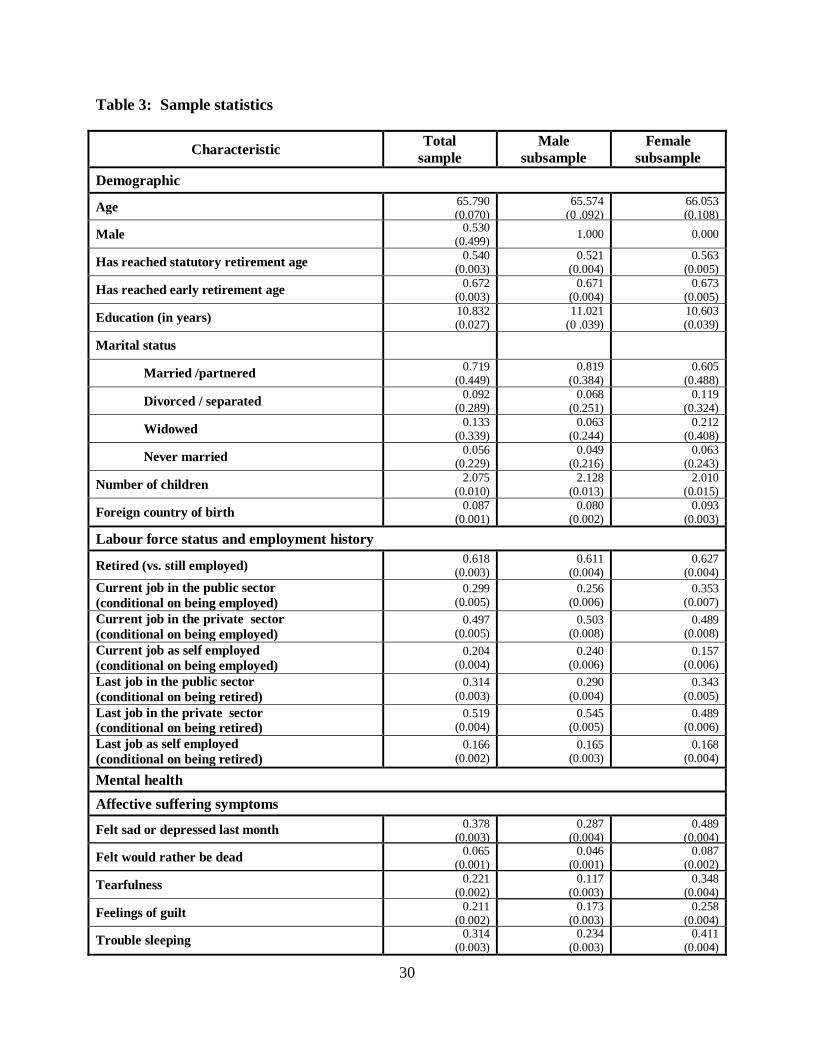
2C. Sample statistics
Table 3 presents the descriptive statistics for the full sample of observations, as well as
for the male and female subsamples separately. 9 The mean age of the persons in the final sample
is 65.8 years, with women being older by 0.5 years (significant at the 1% level). While the
percentage of males and females who have reached early retirement age is roughly the same
(67%), the fraction of women who have reached statutory retirement age is higher by 4.2
percentage points (pp); significant at the 1% level. Women are also less educated by 0.4 years
8 Based on the answer to the question “[…] Looking back over the last 12 months, who are the people with whom
you most often discussed important things? […]”. 9 Means and standard errors corrected for inverse probability weighted sampling; t-test for equality of means with
equal variances reported.
10
and considerably more likely to be widowed – the difference in means equals 0.15; significant at
low levels. Further, the mean number of children of the elderly is 2.1; the gender difference
being statistically different from zero but small in magnitude. To complete the demographic
representation, 9.3% of the females and 8.0% of the males report being born in a country other
than their country of residence.
Next, examining the labour force outcomes of the elderly in SHARE shows that a
somewhat higher fraction of females is retired, but the 1.2pp difference in means is not
significant at the conventional levels. Amongst those who are still working, the highest fraction
reports holding a job in the private sector (roughly 50% of the total sample of employed),
followed by the public sector (30.0%) and self employed individuals (20.4%). Women are more
likely to work in the public sector and significantly less likely to be self employed, and this
pattern holds when looking at the last job history of the retirees, as well.
The lower panel of Table 3 – mental health outcomes – depicts a vivid illustration of the
gender gap in depression in Europe. To elaborate more on this, women are more likely to
experience both the affective suffering symptoms and the demotivation symptoms of depression
(the difference in means being significant at the 1% level for all indicators), resulting in a
considerable gap in the composite Euro-D index of 0.95. The mental health measures exhibiting
highest difference in means (relative to the female sample mean) are tearfulness (0.66), death
ideation (0.47), and trouble sleeping (0.43). It is also worth noting that for both genders feeling
sad or depressed in the last month appears to be the most common affective suffering symptom,
while lack of hopes for the future is the most frequently reported demotivation symptom.
The two groups also differ in their physical health. In particular, women report more
limitations to activities of daily living (0.23 vs. 018 for men) and mobility difficulties (1.79 vs.
1.09), as well as a higher number of chronic conditions (1.63 vs. 1.46); all differences are
statistically significant at the 5% level. In addition, females in the sample are 4.0 pp more likely
to evaluate their health as fair (vs. excellent or very good). Somewhat surprisingly, however,
men appear worse when examining the indicator for hospital stays in the last year, although the
difference is small in magnitude (0.7pp) and significant only at the 10% level.
Turning briefly to the social outcomes of the elderly suggests that, on average, women
have better social and family connectedness – they have broader social networks and are more
likely to keep a close relationship with children and parents. Yet, both groups seem equally
11
satisfied with their social network – the difference in means while statistically significant is low
in magnitude. Lastly, it is interesting to note men take higher participation in volunteering and
charity work, although the difference in means is small in magnitude.
In sum, while the fractions of retired women and men in the sample are comparatively
close, women appear older, more likely to be widowed and to suffer from ill health and,
ultimately, in noticeably poorer psychological condition. This raises an interesting question:
could retirement have a heterogeneous effect on the mental health of the two groups – possibly
adversely affecting females and having a beneficial or no effect for males, or it is the
unfavourable socio-demographic factors (such as loss of a spouse) which induce depressive
suffering for women? Verifying either of the two possibilities requires that the effect of labour
force exit is allowed to vary depending on one’s individual characteristics, as well as on
household characteristics and country-level indicators. We turn to this analysis in the next
section.
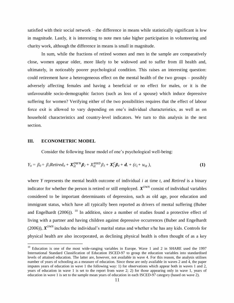
III. ECONOMETRIC MODEL
Consider the following linear model of one’s psychological well-being:
Yit = β0 + β1Retiredit + β2 +
β3 + β4 + dt + ( + ), (1)
where Y represents the mental health outcome of individual i at time t, and Retired is a binary
indicator for whether the person is retired or still employed. XOWN
consist of individual variables
considered to be important determinants of depression, such as old age, poor education and
immigrant status, which have all typically been reported as drivers of mental suffering (Buber
and Engelhardt (2006)). 10
In addition, since a number of studies found a protective effect of
living with a partner and having children against depressive occurrences (Buber and Engelhardt
(2006)), XOWN
includes the individual’s marital status and whether s/he has any kids. Controls for
physical health are also incorporated, as declining physical health is often thought of as a key
10
Education is one of the most wide-ranging variables in Europe. Wave 1 and 2 in SHARE used the 1997
International Standard Classification of Education ISCED-97 to group the education variables into standardised
levels of attained education. The latter are, however, not available in wave 4. For this reason, the analysis utilises
number of years of schooling as a measure of education. Since these are only available in waves 2 and 4, the paper
imputes years of education in wave 1 the following way: 1) for observations which appear both in waves 1 and 2,
years of education in wave 1 is set to the report from wave 2; 2) for those appearing only in wave 1, years of
education in wave 1 is set to the sample mean years of education in each ISCED-97 category (based on wave 2).
12
factor for emotional distress (e.g. Beekman et al. (1997)). Lastly, XOWN
includes sector of
employment at the current/last job as a measure of one’s job characteristics.
Further, XHHD
consists of a household-level control for aggregate annual income
(converted to EUR, PPP-adjusted, and where missing, imputed), and XC incorporates a set of country
dummies accounting for the cross-country differences in depression prevalence (Van de Velde
(2010)). Next, dt denotes year effects to control for the overall economic, public health and
environmental conditions that play a role in one’s mental health (see, e.g., Lavikainen et al.
(2000)), as well as month-of-interview dummies as certain depressive symptoms exhibit a
seasonal pattern. Next, the error component ci represents time-invariant unobserved individual-
level factors that could affect mental health outcomes. One such example is genetic
predisposition, as recent research reported an association between certain genes and various
anxiety and depression disorders (Donner et al. (2008)). Finally, uit is an idiosyncratic error
component reflecting different shocks to one’s mental health, such as stressful life events; e.g.,
illness or death in the family.
A long established econometric concern when studying the effect of retirement on one’s
mental health is the reverse causality between the two – while being retired might possibly
impact one’s mental health, depression may make an individual more likely to exit the labour
force (Conti et al. (2008)). Following the identification strategy developed by Coe and Zamarro
(2011) this paper uses the exogenous variation in the early and statutory retirement ages as
instruments for the state of being retired. Since there are two potential instrumental variables
available, two estimation methods could be employed: pooled instrumental variable (IV)
estimator using either the statutory retirement age or the early retirement age as a single excluded
instrument, and pooled two-stage least squares (2SLS) using both instruments. The later has been
shown to be the most efficient IV estimator under certain assumptions (Wooldridge (2010)).
Formally, the first stage regression in the two-stage least squares (2SLS) estimation has
the following form:
Retiredit = 0 + Zit 1 + 2 +
3 + 4 + dt + it , (2)
where Zit = (Z1it, Z2it) is the vector of excluded instruments. In particular, Z1it denotes a binary
variable for whether person i has reached the statutory retirement age as of time t, and Z2it –
whether s/he has reached the early retirement age at that time. It is worth noting that both
13
instruments vary at cross-country level (as the pension eligibility ages vary between states in the
EU) and at within-country level (based on the individuals’ ages).
There are several identifying assumptions for consistency of the IV/2SLS estimator.
Since the paper involves the use of a binary instrument and a binary instrumented variable,
adopting the notation in the seminal work by Imbens and Angrist (1994) is convenient. Let Yi
denote a vector of all actual mental health outcomes of individual i, and Di denote their actual
retirement outcome (regarded as the treatment). Next, define Yi0 and Yi1 as the potential values of
the outcome of interest when the binary treatment takes on values 0 and 1, respectively, and Di0
and Di1 as the level of the treatment received if the instrument takes on values 0 and 1. In this
way e.g., when the instrument is the statutory retirement age Yit0 stands for the potential mental
health outcome of person i in period t has s/he not reached full retirement age, while Yit1 stands
for the potential mental health of the individual has s/he reached that age. Likewise, Dit0 and Dit1
denote the potential retirement outcomes conditional on the value of the instrument in that time
period.
Under this framework, the first key identifying assumption refers to the relevance of the
instrument(s) and states that conditional on the observable covariates the probability of being
retired should be a non-trivial function of the instrument:
(Di ∣ Zi=k, ∙ ) is a non-trivial function of k, (A1)
where k ∊ {0;1} and ∙ denotes a vector of all covariates from model (1).
In other words, reaching early or statutory retirement age should have an effect on the retirement
propensity.
The second assumption is often referred to as independence of all potential outcomes of
the instrument, or formally:
{Yit0, Yit1, Dit0, Dit1} ⟘ Zit, (A2)
Statement (A2) incorporates two properties of the instrument: exogeneity and
excludability. The first refers to the requirement that the instrument is essentially randomly
assigned with respect to the composite error in that time period (put differently, this requires
14
( )=0 and contemporaneous exogeneity of the instruments (
)=0). 11
Since the early
and full retirement ages are decided at country level, there are no reasons to believe that they are
related to the unobserved heterogeneity at individual level or the idiosyncratic error at that time.
The second part of assumption (A2) captures the restriction that there is no direct link between
the instrument and the outcome of interest. Put differently, the pension eligibility ages should not
be related with an individual’s psychological well-being other than through the state of being
retired. Since the compulsory health insurance scheme in the EU covers major and minor risks
for all employees and retirees, and this coverage does not discontinuously change when reaching
a certain age, be that early or full retirement age,12
one would not expect the instruments to have
a direct effect on a person’s mental health.13
The last assumption requires that the retirement probability is monotonic in the
instruments:
Either Di1 ≥ Di0 ∀i, or Di0 ≥ Di1 ∀i. (A3)
In other words, while reaching early or statutory retirement age may have no effect on some
individuals’ retirement probability, all of those who are affected by the instrument should be
affected in the same direction (also referred to the assumption of “no defiers”). Condition (A3) is
likely to hold; in particular, it is credible that Di1 ≥ Di0 for all i, as there is no reason to believe
any person would be more likely to retire while being below pensionable age but less likely
thereafter.
11 For the countries in SHARE observed at least once, an alternative estimation strategy is available – fixed effects
IV (FEIV). In contrast to pooled 2SLS, which assumes ( )=0 and contemporaneous exogeneity of the
instruments ( )=0, FEIV allows (
)≠0 but imposes the stronger restriction ( )=0, ∀ r, t (strict
exogeneity, see e.g. Wooldridge, 2010). Since the statutory and early retirement ages are decided at country level,
the value of the instruments in each time period only depends on the pensionable ages in a given country and on the
individual’s age at that time period; hence, there is no reason to believe that ( )=0 would fail to hold as ci only
varies at individual level. It is more worrisome, however, to assume that ( )=0 as it would rule out the
possibility that the retirement ages were changed at country level as a response to shocks in the past, which may
have also affected the persons’ mental health. For this reason, pooled 2SLS is the preferred estimation strategy in the
paper. In addition, the Appendix reports the main results when model (1) is estimated under less restrictive
assumptions than the ones imposed by FEIV, namely, fixed effects estimation (see Appendix A1). 12 Source: Healthcare Systems in the EU: a Comparative Study, European Parliament (2010) 13 Given that all countries in the EU set retirement ages to ‘[...] fundamentally follow life expectancy [...] trends’
(European Commission Social Protection Committee Pension Adequacy Report 2010-2050), the statutory and early retirement ages are expected to be linked to the country-average physical health of the elderly. One might worry,
then, that this implies a correlation between an individual’s physical health status and the country pensionable ages
as SHARE is a nationally representative survey and the national-average physical health depends on each
individual’s health status. However, even if excludability is an issue of concern when the outcome is individual’s
physical health, it is not likely to be the case when studying the effect of retirement on depression of outpatients
(mental illness has been shown to lower life expectancy for inpatients due to the detrimental physical health effect of
antipsychotic medication; see e.g. Crystal et al. (2009)).
15
Under assumptions (A1) through (A3), the IV estimand captures the local average
treatment effect (LATE), i.e., it identifies the average treatment effect of retirement on mental
health for the subpopulation of retirees whose retirement was induced by the instrument. It is
evident from here that this effect need not be the same when employing the early and statutory
retirement age as an instrument since the groups affected by each of these instruments are
different.
IV. ESTIMATION RESULTS
4A. First stage
4A.1. Statutory and early retirement ages, and actual retirement ages in SHARE
Table 4 shows the statutory, early and actual mean retirement ages in SHARE for each
country in the sample, separately for waves 1-2 and wave 4.14
Several observations are worth
noting at this point. First, even though there has been some convergence of the statutory
retirement ages towards age 65 and the early retirement ages towards age 60, some cross-country
variation in those ages still exists. Secondly, on average, the post transition economies provide
access to early and full retirement considerably earlier than the EU-15 and Switzerland; in
addition, the new EU members are more likely to maintain different pensionable ages for women
and men.
Furthermore, although not a perfect predictor of the actual ages of retirement, statutory
and early retirement ages do have “bite”. For instance, the country with highest statutory
retirement age in Europe is Sweden, setting the full retirement age at 67 as of 2010, and it is also
the country with highest actual retirement ages for men and one of the highest for women. Next,
an increase of the statutory retirement age appears to result in an increase of the actual age of
retirement: e.g., Italy increased this age for women from 60 to 65 years following wave 2, and
saw an increase of the mean female’s retirement age in the sample from 57 to 58.1 years –
considerably higher than the increase for men (0.5 years). Finally, while women tend to retire
earlier in all countries, the gender differential in the mean retirement ages is lower for countries
14 The question about year of retirement was asked in waves 2 and 4 only. Year of retirement imputed for the retired
individuals in wave 1 based on the report from wave 2. Retirement age derived as the difference between year of
retirement and year of birth.
Waves 1 and 2 are grouped together as the main sources of information for the early and statutory retirement ages in
years 2004 and 2007 report no changes in those in the period.
16
with equal treatment of women and men; for instance, for wave 4, this differential was 2.7 years
in Poland but only 0.1 years in Sweden.
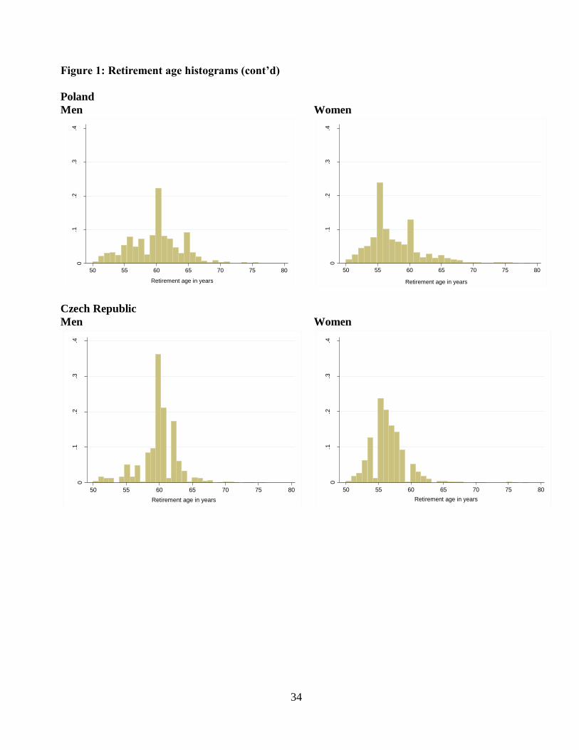
To further illustrate the link between the legislative provisions for retirement and the
actual ages of retirement, it is also useful to examine the entire histogram of the ages of labour
force exit. Figure 1 shows these histograms for four of the countries in the SHARE sample –
Sweden and Switzerland selected amongst the states with high statutory and early retirement
ages, and the Czech Republic and Poland amongst those with low eligibility ages. It is apparent
that the largest fractions of women and men in Sweden, which has equal treatment for both
genders, retire at the pre-2010 statutory retirement age, and the two histograms exhibit very
similar patterns. Males in Switzerland also appear most likely to exit from labour when reaching
full retirement age (65 years), while the largest fraction of females stops working at the early
retirement age (62 years), followed by relatively equal shares of retirees at age 63 and the full
retirement age, 64. Turning to the post-transition countries, the retirement probabilities in Poland
display a clear peak at the (pre-2009) early retirement age for both genders, followed by a
secondary peak at the respective statutory retirement ages. Lastly, while most men in the Czech
sample exit the labour force at the single early retirement age, 60, the retirement probabilities for
females are high, albeit declining, for all ages 55 through 59, likely due to the linkage of
retirement eligibility to number of children. Overall, these examples strongly confirm that the
early and statutory retirement ages strongly influence the distribution of retirement ages.
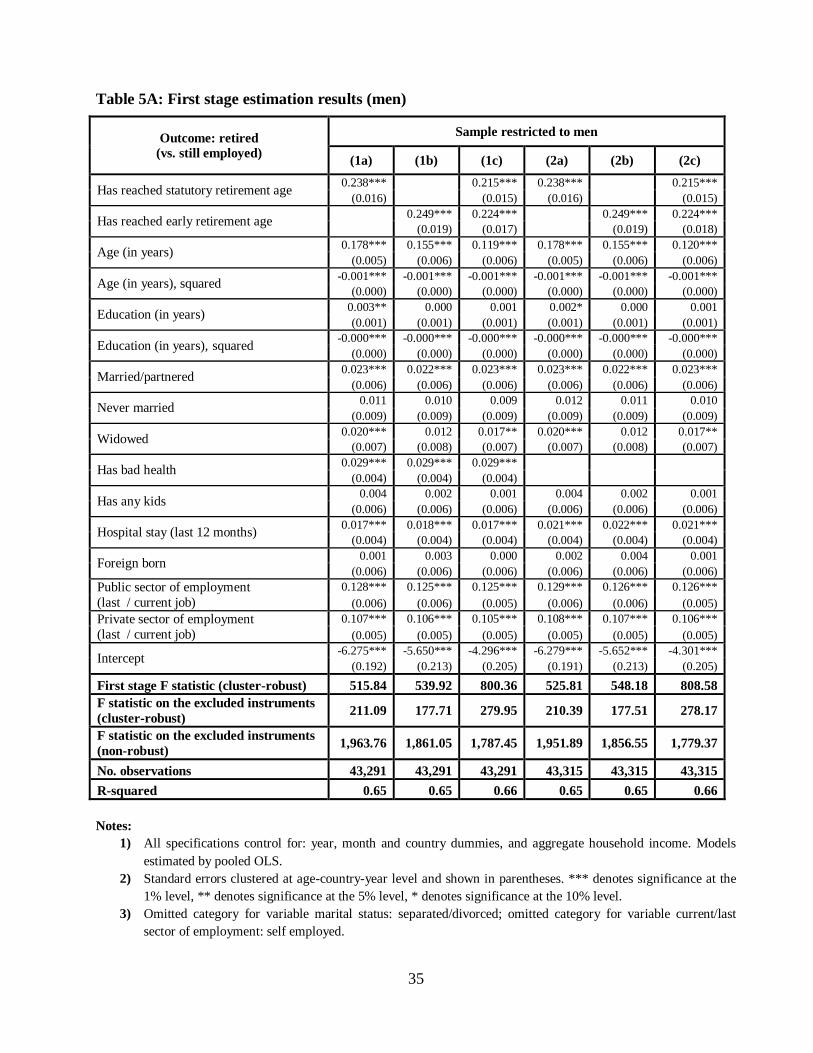
4A.2. Estimation results
Tables 5A and 5B report the first stage estimation results separately for the male and
female subsamples. Column (1a) reports estimates from Model (2) using the statutory retirement
age as a single excluded instrument, column (1b) uses the early retirement age only, and column
(1c) uses both instruments. Columns (2a-2c) repeat the specifications but add a binary indicator
for being in bad health; this measure is potentially endogenous to mental health, but we include it
to assess its effect on the estimated treatment effect of interest.
As can be seen from the table, the statutory and the early retirement ages are strong
predictors of retirement for both genders. For instance, column (1a) of Table (5A) implies that
having reached statutory retirement age on average increases the probability that a male has
retired by 23.8 pp, ceteris paribus, and the effect is highly significant. The corresponding
17
specification from Table 5B states that reaching full retirement age would make a female 28.8 pp
more likely to exit the labour force, other factors being equal. The early retirement age is also
estimated to induce retirement with a high probability for both men and women (magnitudes of
0.25 and 0.28, respectively), and the effects are statistically different than zero at low levels.
Essentially the same conclusions prevail when both instruments are employed, and the models
are robust to the exclusion of the bad health indicator. It is also interesting to note that age
appears a significant predictor of exiting work, even after accounting for reaching full and early
retirement age.
Lastly, it is useful to examine the first stage F-statistic and the F-statistic on the excluded
instruments as suggested by several studies (see, e.g., Stock and Yogo (2005)). In particular, a
number of authors reported a correspondence between the first stage F-statistic and the bias of
the IV estimator relative to the bias of the OLS estimator, and some proposed rules of thumb for
evaluating the relevance of the instruments. For instance, Staiger and Stock (1997) suggested an
F-statistic on the excluded instruments of at least 10. The lower panel of Tables 5A and 5B
reports the non-robust and the cluster-robust F-statistic of the regression – they are considerably
higher than 10 in all specifications.15
4B. Second stage
4B.1. Mental health by age distance to statutory and early retirement
Figure 2 illustrates the pattern of the mental health indicators16
for all men and women in
the sample by age distance to statutory retirement age; in addition, the fractions of employed
males/females in each age group are presented. The graphs for women (depicted on the left-
hand-side panels) show that the most sizeable drop in the females’ employment probability
occurs two years prior to reaching statutory retirement age, when this probability declines by
15pp. In addition, a large fraction of women exit from work one year before full retirement age
and the year when this age is reached. For men (right-hand side graphs), the majority of
15
The critical values and rules of thumb for the F-statistic on the excluded instruments are based on the assumption
of i.i.d. errors. Since SHARE collects household-level country data, heteroskedasticity and serial correlation are
likely to be present; for this reason, the tables also report the cluster-robust F-statistic on the excluded instruments.
The related theoretical results do not extend to proposing critical values for the robust F-statistic but a recent study
by Bun and De Haan (2010) used simulations and showed that a decrease in the robust F-statistic is enough to offset
the increase in the IV bias relative to OLS; in other words, even values lower than 10 would suffice.
16 The graphs do not look at the indicator for feeling sad or depressed during the month preceding the interview as
this measure is particularly likely to exhibit seasonal patterns.
18
retirements occur two years prior to statutory age (12% decline in the share of working males),
followed by considerable drops in employment at the full retirement age and the year after.
Panels A and B of Figure 2 show the mean death ideation by age category for women and
men, respectively. Focusing on the changes that occur around the statutory retirement age reveals
a large improvement in this indicator for women in the years before reaching statutory retirement
age when females’ employment marks its most sizeable decline. Death ideation somewhat
increases at the cut-off; nevertheless, its mean remains at a lower level two years after full
retirement age, before gradually increasing thereafter. For men, suicidal wishing is characterised
by a large jump at the cut-off and no drop prior to it; in addition, the decline in this measure
following full retirement age is mirrored by an almost equally sized increase the year after. Next,
Panels C and D illustrate the patterns of the demotivation measure: while this index sees a
sizeable drop for females a year before reaching statutory retirement, the index for men remains
mostly unchanged around the cut-off. Turning to the affective suffering index (Panels E and F)
shows a large decline in this measure in the years around the cut-off for women, while the
improvement for men is not as striking. Lastly, the patterns in the Euro-D scale (Panels G and
H), point towards a substantial decline for women around the statutory retirement age, while
suggesting only a minor favourable development for men.
Figure 3 illustrates the analogous graphs for both genders by distance to early retirement
age. The largest proportion of women in SHARE tends to retire when they are first eligible for
early retirement (the fraction employed declining by nearly 15 pp at the cut-off). In contrast, the
majority of men exit work two years after early retirement age when their employment
probability marks a 13 pp decline. The pattern of the mean death ideation for women (Panel A)
depicts an improvement when early retirement age is reached and the year after, and only a
minor increase during the following six years. There is a parallel drop in this mental health
measure for men, as well (Panel B), occurring two years after early retirement age – the age
when most male workers retire; however, males’ death ideation remains at a lower level for just
two years, increasing sharply thereafter. Examining the demotivation index (Panels C and D)
also suggests an improvement for both genders at the time when the fractions of employed
elderly decline most, with this improvement being more pronounced for females. The patterns of
the affective suffering index and the Euro-D scale are essentially the identical at the cut-off: a
large and sustained decline for women and only a temporary drop for men; the male indices also
19
improve two years after reaching early retirement. Finally, for both genders all mental health
measures exhibit a nearly linear upward trend starting right after retirement eligibility age.
4B.2. Estimation results
Mental health
As shown in the previous section, both instruments – the statutory and the early
retirement age – are strong predictors of retirement. In the absence of weak instrument concerns
the 2SLS estimator combining both IVs provides efficiency gains; for this reason, the main part
of the subsequent analysis focuses on the estimation results when using both instruments, but we
will also examine second stage results based on each instrument separately.
Table 6A and 6B report these results for men and women, respectively, when the mental
health outcome of interest is whether the person had suicidal thoughts. The leftmost panel of
Table 6A shows the pooled OLS estimates for the male sample when model (1) includes controls
for age, time and country dummies only (specification (1a), as well as when employing all
covariates (specification (1b). Due to suspected endogeneity of the binary indicator for being in
bad health, column (1c) reports the estimation results when omitting this variable. As can be seen
from here, the pooled OLS estimates suggest a statistically significant detrimental impact of a
male’s retirement on death ideation, ceteris paribus. In contrast, panels (2) to (4) report the
parameter estimates when employing an instrumental variable estimation on the same
specifications as in Panel (1). The key implication from this set of results is that once
endogeneity of retirement is accounted for, a male’s labour force exit does not play an important
role in the occurrence of suicidal thoughts – the coefficient on retirement appears negative in
sign but insignificantly different from zero in all but one specification. The only exception is the
2SLS estimate from column (4a) when both instruments are employed – it is negative 0.018 and
marginally significant, but it drops in magnitude and significance once covariates are included in
specifications (4b) and (4c).
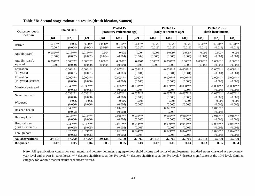
Table 6B reports the corresponding estimation results for the female sample. As before,
the pooled OLS estimates on retirement exhibit an upward bias, although the coefficients are
somewhat smaller in magnitude and significance than the ones obtained on the male sample.
Columns (2a) to (2c) report the results when employing the statutory retirement age as an
instrument for retirement, and the parameters on retirement have the interpretation of an average
20
treatment effect for the female subpopulation of compliers with the full retirement age. These
results imply that for women whose labour force exit is induced by the statutory retirement age,
retirement reduces the occurrence of suicidal thoughts by nearly 4pp, ceteris paribus, and the
effect is statistically significant at the 5% level. Next, specifications (3a) to (3c) report the
estimation results on the female subsample when the early retirement age is employed as the
single excluded instrument. In these specifications, the parameters on retirement are still negative
in sign but lower in magnitude and less precisely estimated, implying no important effect of
labour force exit on death ideation for the women whose retirement is induced by the early
retirement age. Further, the rightmost panel of table 6B reports the 2SLS results when both
instruments are used; the average treatment effect of retirement for both groups of compliers is
roughly negative 0.03, implying a beneficial effect of labour force exit on suicidal thoughts for
these women (also note the considerably lower standard errors on the estimates illustrating the
efficiency gain of pooled 2SLS compared to pooled IV). Lastly, it is worth noting that compared
to the female sample mean of the death ideation indicator, 0.087, the estimated magnitude of the
effect of retirement of 0.03 is very large.
Taken as a whole, the estimation results examined so far suggest a large and significant
beneficial effect of retirement on death ideation for women but no corresponding effect for men.
In addition, although this impact is significant when looking at both groups of compliers as
shown by the 2SLS results, it does seem stronger for the compliers with the statutory retirement
age. The next sections shall focus on the 2SLS estimation results in order to make use of the
efficiency gain when employing both instruments and aiming at reporting an average treatment
effect for both groups of compliers.
Table 7 shows the estimation results on the parameter of interest for all the remaining
mental health measures. When the outcome is the composite demotivation index (the later
ranges from 0 to 4, where higher values imply worse psychological well-being), the pooled OLS
estimates on retirement for men (reported in Panel A) are positive and highly significant in all
specifications. However, once retirement is instrumented by the statutory and early retirement
ages, the key parameter of interest appears negative in sign and not statistically different from
zero in all specifications. Turning to panel B, the pooled OLS estimates overall imply a
detrimental effect of retirement on the composite demotivation index for women; yet, once a
2SLS estimator is employed, the impact of retirement for the females complying with the
21
instruments appears negative in sign and statistically significant at low levels across all
specifications. For instance, the estimate from column (2b), obtained when including all
covariates, is -0.187, implies that, other factors equal, labour force exit has a beneficial effect on
the demotivation index for women (interpreted as a local average treatment effect). Moreover,
the magnitude of this effect is very large – roughly one-third of the female sample mean for this
mental health indicator.
The next section of Table 7 reports the second stage results for the effect of retirement on
the affective suffering index (scale ranging from 0 to 8). As can be seen from here, both sets of
estimation results tell a similar story – while the pooled OLS estimator implies that retirement
increases the occurrence of affective suffering symptoms both for women and for men, the
pooled 2SLS estimator suggests that labour force exit has no important impact on this composite
mental health index for either gender.
Table 7 also illustrates the estimation results when the outcome of interest is the Euro-D
index. As before, the pooled OLS estimates on retirement are positive and significant for both
genders, meaning that exiting the workforce worsens one’s psychological well-being, ceteris
paribus. 2SLS leads to entirely different conclusions, namely that retirement plays no significant
role in determining the Euro-D index for men, but it has a favourable effect for women. The
magnitude of this effect is non-negligible (0.24, based on the specification with covariates),
compared to the female sample mean of the Euro-D scale, 2.78.
Lastly, we examine the results when the mental health outcome variable is a dummy for
feeling sad or depressed in the month preceding the interview (reported in the lowest section of
each panel of Table 7). In short, while the pooled OLS estimator suggests a detrimental effect of
retirement, the 2SLS estimates imply that retirement is not a significant predictor of the
occurrence of sadness and depression episodes, either for women or for men. 17
17
The same identification strategy could be employed to investigate the presence of spousal retirement cross-effects
amongst the couple households in SHARE (21,528 couple observations). Treating spousal retirement as endogenous
and instrumenting both own and spousal retirement (the later by whether spouse has reached full and early
retirement age, and controlling for spousal age) reveals that, conditional on own retirement, spousal retirement has
no significant impact on one’s own mental health. It is also important to note that the gender heterogeneity in the
effect of retirement holds when restricting the attention to couple household only – retirement significantly reduces
women’s death ideation (magnitude of the effect negative 0.37 in the specification with covariates) and
demotivation index (magnitude negative 0.135 in the specification with covariates), while having no effect for men.
22
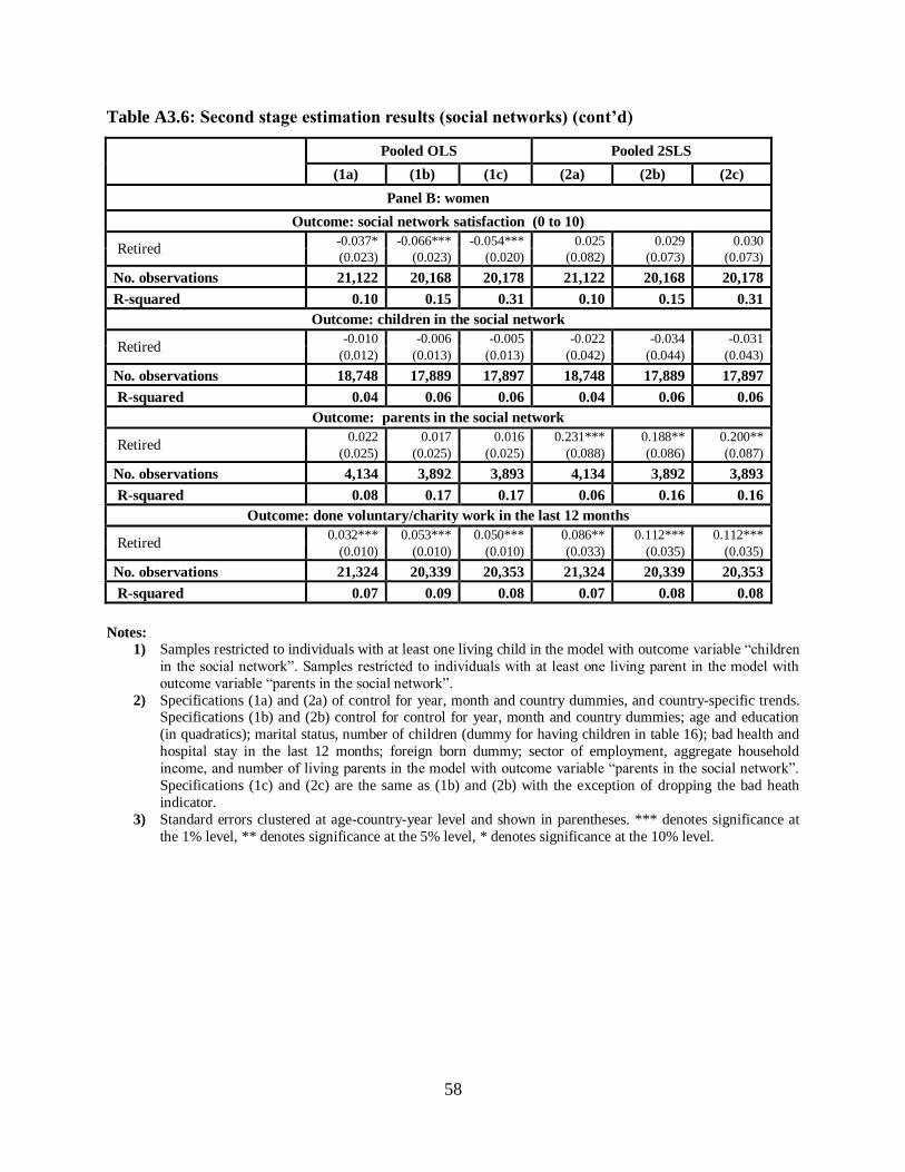
Social networks
This subsection of the paper uses the last wave in SHARE to estimate model (1) when the
dependent variable represents a social outcome of interest rather than mental health. In
particular, Yit represents the size and satisfaction with one’s social network; number of persons in
the network with daily contact; a binary indicator for children and parents present in the network,
as well as participation in voluntary work. All covariates are the same as before, except that
vector XOWN
includes number of children rather than a dummy for having kids in all
specifications but the one for volunteering, and an additional control for number of living parents
when the dependent variable is presence of a parent in the respondent’s social network. The
model is estimated using the identification strategy described in section III in order to account
for the reverse causality between retirement and social outcomes. To elaborate more on this,
prior studies report that labour force exit reduces social contacts and induces social isolation
(Sugisawa et al. (1997)), while at the same time social networks and interactions have been
found to be significant determinants of a worker’s retirement decision (Duflo and Saez (2003)).
Since both the statutory and the early retirement ages are likely exogenous in a model of social
outcomes and affect those outcomes only through retirement, employing them as instruments for
retirement becomes an attractive estimation strategy.
The top section of Table 8 (panels A and B for men and women, respectively) report the
estimation results when the outcome of interest is the number of persons in a respondent’s
immediate social network. As can be seen from here, once reverse causality between the size of
one’s social network and the decision to exit the labour force is accounted for, retirement
decreases the number of persons in a male retiree’s network by roughly 0.20 (compared to a
sample mean of 2.28), while there is no analogous effect for females. A somewhat similar
suggestion of an adverse effect of retirement on social contacts for men can be drawn based on
the next section of Table 8, panel A. Specifically, the 2SLS results from column (2a) imply that
exiting work lessens the number of persons with daily contact amongst a male’s social network,
ceteris paribus, although, this effect is not different from zero at low significance levels once
other covariates are included. Again, there is no corresponding effect for women (panel B). At
the same time, Table 8 also suggests that retirement has no significant impact on the overall
satisfaction of the elderly with their social network – the parameter on retirement is low in
magnitude and significance for both genders.
23
The next two sets of regressions look at the effect of labour force exit on child-parent
bonding. In particular, Table 8 reports the results from estimating model (1) on a restricted
sample of elderly with at least one living child, when the outcome of interest is a binary indicator
for presence of children in one’s social network. The estimates imply that being a retired parent
is not an important predictor of keeping a relationship with one’s kids, either for women or for
men. Further, Tables 8 shows the estimation results when the dependent variable is a dummy for
presence of a parent in the social network (based on the subsample of respondents with at least
one living parent). Those results reveal that retirement significantly increases the probability that
a female keeps contact with a parent by roughly 19pp, ceteris paribus. There is also some
tentative evidence that men are more likely to have a parent in their social network once they exit
work (column (2a) of panel A), but this effect drops in magnitude and significance once controls
are included.
Lastly, we examine the effect of retirement on an important social activity of the elderly –
volunteering. The central implication from Table 8 is that labour force exit significantly
increases the probability of involvement with voluntary or charitable work for both genders,
ceteris paribus. The magnitude of this effect is 0.08 for males and 0.11 for females (based on the
specifications will all covariates). This comprises large effects compared to the sample means of
voluntary work (0.18 for men and 0.16 for women, respectively).
4C. More on the gender heterogeneity and mechanism of the effect
In order to complete the discussion on the gender heterogeneity of the effect of retirement
Tables 9 presents a test for equality of the parameter on retirement in model (1) by gender; in
other words, they report the results from testing the hypothesis H0:
= As can be
seen from here, the effect of retirement on one’s demotivation index is significantly different for
men and women: the bootstrap estimates of this difference are large in magnitude and
statistically significant (significance at the 1% level in the model with no controls, and at the 5%
level in the specifications with covariates). At the same time, however, the test cannot reject the
null that the coefficient on retirement is the equal for both genders when the outcome of interest
is any other psychological well-being measure, or a measure of the social connectedness of the
elderly (in the later case the comparison is further complicated by the reduced sample size and
lower estimation precision). Overall, this provides further support for the idea of gender
24
heterogeneity of the effect of labour force exit on mental health measured by the composite
demotivation index.
Before concluding, the paper addresses an issue which has been largely overlooked by
previous research: does the mechanism of the effect of retirement on one’s mental health go
through their social network? This may be the case as retirement was shown to affect the social
connectedness of the elderly – it narrows down a male retiree’s social network, while having no
effect for females, which may potentially explain why labour force exit appears beneficial for
women’s mental health but not for men’s. In addition, females in the sample have better social
connectedness overall, and better relations with children in particular, both of which have been
hypothesised to lower depression rates. Lastly, exiting work was revealed to increase
volunteering of the elderly, which has in turn been linked to lower depression rates (Lum and
Lightfood (2005)). We proceed by estimating model (1) from section III on the last wave of data
and include a number of social inclusion measures, such as size of the social network, children in
the network and volunteering. We then examine the resulting change in the estimated effect of
retirement, compared to the model with no controls for social networks.
The results are reported in Tables 10A and 10B. It is evident that the model is robust to
inclusion of social network size and presence of children in the network for both genders.
However, the parameter on women’s retirement drops both in magnitude and in significance
when volunteering is included in the regressions for the demotivation and Euro-D measures
(columns (2d) and (3d) of Table 10B), but not in the model for death ideation. For the male
sample, the effect of labour force exit on the death ideation and demotivation index also changes
in significance once volunteering is controlled (column (2d) of Table 10A); yet, the magnitude of
these changes is essentially zero.
Based on the above results, this paper fails to find any evidence that the effect of
workforce exit on a person’s mental health goes through altering their social network; however,
the analysis suggests that, at least in part, the beneficial effect of retirement on the composite
Euro-D and demotivation indices for women is explained by the increase in volunteering
following their labour force exit.
25
CONCLUDING REMARKS
This study utilised household-level multinational data from 17 countries in Europe to
explore the effects of labour force exit on the mental health of the elderly. Following the
identification strategy developed by Coe and Zamarro (2011) the paper explored the exogenous
variation in the retirement propensity of the older workers, induced by the national statutory and
early retirement ages. Consistent with the findings of Coe and Zamarro (2011) the analysis
presented here provides support for the idea that retirement has no significant impact on men’s
psychological well-being, other factors being equal. At the same time, however, this study finds
evidence for a beneficial effect of retirement on women’s emotional health, which is an
important contribution to the literature. In particular, exiting the workforce is predicted to
decrease the likelihood that a female has suicidal thoughts by about 3pp, ceteris paribus, and to
improve her mental health as measured by the composite demotivation and Euro-D depression
scores. The magnitude of this effect is large for the death ideation and demotivation indicators,
while relatively low for the Euro-D index. Lastly, there is no evidence that retirement plays an
important role on the occurrence of a recent depressive episode and on the composite affective
depression measure for either gender.
The central estimates also uncover a role for retirement on the social contacts of older
adults. In particular, the analysis presented evidence that exiting work decreases the size of the
immediate social network for male retirees (in agreement with the findings of Sugisawa et al.
(1997)) with no corresponding effect for women. Moreover, retirement significantly increases
the probability of a parent present in the social network for females, but not for males. Lastly, the
paper found no evidence that retirement induces self-perceived social isolation – exit from work
has no significant impact on one’s overall satisfaction with their social network, and has a
beneficial effect on volunteering for both genders.
The implications of these findings are twofold. First, the gender heterogeneity of the
effect of retirement on mental health and social networks is in line with contemporary theories in
the psychology literature suggesting a differential impact of employment on a female’s and a
male’s emotional well-being. Secondly, the results in this paper have potentially important policy
implications. Specifically, the lack of an important impact of labour force exit on men’s
psychological health implies that the recent trends in the EU towards increasing the statutory and
early ages of retirement would lead to no detrimental consequences for their mental health, and
26
may have a favourable impact on their social connectedness. At the same time, however, the
existence of a beneficial effect of retirement on women’s psychological well-being and
relationship with parents, cannot rule out the possibility that increasing the pensionable ages – as
well as equalizing those ages across gender – would lead to a loss of social welfare for women.
27
References
Atchley, Robert C. "Continuity theory, self, and social structure." The self and society in aging processes 94
(1999): 121.
Balleer, Almut, Ramón Gómez-Salvador, and Jarkko Turunen. Labour force participation in the euro area: a
cohort based analysis. No. 1049. European Central Bank, 2009.
Barnes, Helen, and Jane Parry. "Renegotiating identity and relationships: Men and women's adjustments to
retirement." Ageing and Society 24, no. 02 (2004): 213-233.
Beck, Scott H. "Adjustment to and satisfaction with retirement." Journal of Gerontology 37, no. 5 (1982): 616-624.
Beekman, A. T. F., B. W. J. H. Penninx, D. J. H. Deeg, J. Ormel, A. W. Braam, and W. Van Tilburg. "Depression
and physical health in later life: results from the Longitudinal Aging Study Amsterdam (LASA)." Journal of
affective disorders 46, no. 3 (1997): 219-231.
Bonsang, Eric, and Tobias Klein. "Retirement and subjective well-being." Journal of Economic Behavior &
Organization (2012).
Bound, John, and Timothy Waidmann. "Estimating the health effects of retirement." Michigan Retirement
Research Center Research Paper No. UM WP 168 (2007).
Buber, Isabella, and Henriette Engelhardt. "Children’s impact on the mental health of their older mothers and
fathers: findings from the Survey of Health, Ageing and Retirement in Europe." European Journal of Ageing 5, no. 1 (2008): 31-45.
Castro-Costa, Erico, Michael Dewey, Robert Stewart, Sube Banerjee, Felicia Huppert, Carlos Mendonca-Lima,
Christophe Bula et al. "Prevalence of depressive symptoms and syndromes in later life in ten European countries
The SHARE study." The British Journal of Psychiatry 191, no. 5 (2007): 393-401.
Charles, Kerwin Kofi. "Is retirement depressing?: Labor force inactivity and psychological well-being in later life."
Research in Labor Economics 23 (2004): 269-299
Clark, Andrew E., and Yarine Fawaz. "Valuing jobs via retirement: European evidence." National Institute
Economic Review 209, no. 1 (2009): 88-103.
Coe, Norma B., and Gema Zamarro. "Retirement effects on health in Europe." Journal of health economics 30,
no. 1 (2011): 77-86.
Conti, Rena M., Ernst R. Berndt, and Richard G. Frank. Early retirement and public disability insurance applications: Exploring the impact of depression. No. w12237. National Bureau of Economic Research, 2006.
Copeland, J. R. M., Michael E. Dewey, and H. M. Griffiths-Jones. "A computerized psychiatric diagnostic system
and case nomenclature for elderly subjects: GMS and AGECAT." Psychological medicine 16, no. 01 (1986): 89-99.
Coursolle, Kathryn M., Megan M. Sweeney, James M. Raymo, and Jeong-Hwa Ho. "The Association Between
Retirement and Emotional Well-being: Does Prior Work–Family Conflict Matter?." The Journals of Gerontology
Series B: Psychological Sciences and Social Sciences 65, no. 5 (2010): 609-620.
Crystal, Stephen, Mark Olfson, Cecilia Huang, Harold Pincus, and Tobias Gerhard. "Broadened use of atypical
antipsychotics: safety, effectiveness, and policy challenges." Health Affairs 28, no. 5 (2009): w770-w781.
Dave, Dhaval, Inas Rashad, and Jasmina Spasojevic. The effects of retirement on physical and mental health
outcomes. No. w12123. National Bureau of Economic Research, 2006.
DG-ECFIN, E. C. "The 2009 Ageing Report: economic and budgetary projections for the EU-27 Member States
(2008–2060)." Joint Report prepared by the European Commission (DG ECFIN) and the Economic Policy Committee (AWG). Luxembourg: Office for Official Publications of the European Communities (2009).
Diener, Ed, Ed Sandvik, Larry Seidlitz, and Marissa Diener. "The relationship between income and subjective well-
being: Relative or absolute?." Social Indicators Research 28, no. 3 (1993): 195-223.
28
Donner, Jonas, Sami Pirkola, Kaisa Silander, Laura Kananen, Joseph D. Terwilliger, Jouko Lönnqvist, Leena
Peltonen, and Iiris Hovatta. "An association analysis of murine anxiety genes in humans implicates novel candidate
Duflo, Esther, and Emmanuel Saez. Implications of information and social interactions for retirement saving
decisions. Pension Research Council Working Paper 2003-13, Philadelphia, 2003.
European Commission. "Pension adequacy in the European Union 2010-2050." Report prepared jointly by the Directorate-General for Employment, Social Affairs and Inclusion of the European Commission and the Social
Protection Committee (2012).
European Parliament. "Healthcare Systems in the EU: a Comparative Study.", Directorate General for Research,
Imbens, Guido W., and Joshua D. Angrist. "Identification and estimation of local average treatment effects."
Econometrica 62, no. 2 (1994): 467-475.
Lavikainen, Juha, Eero Lahtinen, and Ville Lehtinen, eds. Public health approach on mental health in Europe.
Stakes, 2000.
Lennon, Mary Clare, and Sarah Rosenfield. "Women and mental health: the interaction of job and family
conditions." Journal of health and social behavior (1992): 316-327.
Lum, Terry Y., and Elizabeth Lightfoot. "The effects of volunteering on the physical and mental health of older people." Research on aging 27, no. 1 (2005): 31-55.
Mead, George Herbert. Mind, self, and society: From the standpoint of a social behaviorist. University of Chicago
press, 2009.
Mirowsky, John. "Age and the gender gap in depression." Journal of Health and Social Behavior (1996): 362-380.
O'Riley, Alisa A., Kimberly A. Van Orden, Hua He, Thomas M. Richardson, Carol Podgorski, and Yeates Conwell.
"Suicide and death ideation in older adults obtaining aging services." The American Journal of Geriatric Psychiatry
(2013).
Portnoi, V. A. "Postretirement depression: myth or reality." Comprehensive therapy 9, no. 7 (1983): 31.
Prince, Martin J., A. T. Beekman, D. J. Deeg, R. Fuhrer, S. L. Kivela, B. A. Lawlor, A. Lobo et al. "Depression
symptoms in late life assessed using the EURO-D scale. Effect of age, gender and marital status in 14 European
centres." The British Journal of Psychiatry 174, no. 4 (1999): 339-345.
Salami, Samuel O. "Retirement context and psychological factors as predictors of well-being among retired
teachers." Europe’s Journal of Psychology 6, no. 2 (2010): 47-64.
Staiger, Douglas, and James H. Stock. "Instrumental variables regression with weak instruments." Econometrica
65, no. 3 (1997): 557-586.
Stock, James, and Motohiro Yogo. Asymptotic distributions of instrumental variables statistics with many
instruments. Vol. 6. Chapter, 2005.
Sugisawa, Atsudo, Hidehiro Sugisawa, Yomei Nakatani, and Hiroshi Shibata. "Effect of retirement on mental
health and social well-being among elderly Japanese" [Nihon koshu eisei zasshi] Japanese journal of public health
44, no. 2 (1997): 123-130.
Tibbitts, Clark. "Retirement problems in American society." American Journal of Sociology (1954): 301-308.
Van de Velde, Sarah, Piet Bracke, and Katia Levecque. "Gender differences in depression in 23 European
countries. Cross-national variation in the gender gap in depression." Social Science & Medicine 71, no. 2 (2010): 305-313.
Wooldridge, Jeffrey M. Econometric analysis of cross section and panel data. The MIT press, 2002.
29
Table 1: Country representation
Country Fraction of total sample
wave 1 wave 2 wave 4
Austria 0.068 0.037 0.092
Germany 0.117 0.082 0.026
Sweden 0.141 0.106 0.037
Netherlands 0.088 0.068 0.039
Spain 0.062 0.049 0.041
Italy 0.081 0.079 0.052
France 0.117 0.093 0.100
Denmark 0.071 0.093 0.044
Greece 0.090 0.083 NA
Switzerland 0.040 0.048 0.070
Belgium 0.124 0.084 0.080
Czech Republic NA 0.108 0.125
Poland NA 0.070 0.024
Hungary NA NA 0.053
Portugal NA NA 0.034
Slovenia NA NA 0.047
Estonia NA NA 0.136
Total 18,632 22,257 40,934
Table 2: Labour force status by gender
Note: sample restricted to individuals for whom the main variables of interest are not missing.
Labour force status Number of observations Employment / retirement rate
Males Females Total Males Females Total
Employed 16,372 14,610 30,982 37.7% 38.0% 37.9%
Retired 27,028 23,813 50,841 62.3% 62.0% 62.1%
Total 43,400 38,423 81,823 100.00% 100.0% 100.0%
30
Table 3: Sample statistics
Characteristic Total
sample
Male
subsample
Female
subsample
Demographic
Age 65.790
(0.070) 65.574
(0 .092) 66.053
(0.108)
Male 0.530
(0.499) 1.000 0.000
Has reached statutory retirement age 0.540
(0.003) 0.521
(0.004) 0.563
(0.005)
Has reached early retirement age 0.672
(0.003) 0.671
(0.004) 0.673
(0.005)
Education (in years) 10.832
(0.027) 11.021
(0 .039) 10.603
(0.039)
Marital status
Married /partnered 0.719
(0.449) 0.819
(0.384) 0.605
(0.488)
Divorced / separated 0.092
(0.289) 0.068
(0.251) 0.119
(0.324)
Widowed 0.133
(0.339) 0.063
(0.244) 0.212
(0.408)
Never married 0.056
(0.229) 0.049
(0.216) 0.063
(0.243)
Number of children 2.075
(0.010) 2.128
(0.013) 2.010
(0.015)
Foreign country of birth 0.087
(0.001) 0.080
(0.002) 0.093
(0.003)
Labour force status and employment history
Retired (vs. still employed) 0.618
(0.003) 0.611
(0.004) 0.627
(0.004)
Current job in the public sector
(conditional on being employed)
0.299 (0.005)
0.256 (0.006)
0.353 (0.007)
Current job in the private sector
(conditional on being employed)
0.497 (0.005)
0.503 (0.008)
0.489 (0.008)
Current job as self employed
(conditional on being employed)
0.204 (0.004)
0.240 (0.006)
0.157 (0.006)
Last job in the public sector
(conditional on being retired)
0.314
(0.003)
0.290
(0.004)
0.343
(0.005)
Last job in the private sector
(conditional on being retired)
0.519 (0.004)
0.545 (0.005)
0.489 (0.006)
Last job as self employed
(conditional on being retired)
0.166 (0.002)
0.165 (0.003)
0.168 (0.004)
Mental health
Affective suffering symptoms
Felt sad or depressed last month 0.378
(0.003) 0.287
(0.004) 0.489
(0.004)
Felt would rather be dead 0.065
(0.001) 0.046
(0.001) 0.087
(0.002)
Tearfulness 0.221
(0.002) 0.117
(0.003) 0.348
(0.004)
Feelings of guilt 0.211
(0.002) 0.173
(0.003) 0.258
(0.004)
Trouble sleeping 0.314
(0.003) 0.234
(0.003) 0.411
(0.004)
31
Table 3: Sample statistics (cont’d)
Characteristic Total
sample
Male
subsample
Female
subsample
Loss of appetite 0.074
(0.001) 0.060
(0.002) 0.091
(0.002)
Irritability 0.277
(0.003) 0.263
(0.004) 0.294
(0.004)
Fatigue 0.316
(0.003)
0.266
(0.004)
0.377
(0.004)
Affective suffering symptoms index (0 to 8) 1.731
(0.012) 1.343
(0.013) 2.202
(0.019)
Demotivation symptoms
Pessimism (no hopes for the future) 0.157
(0.002) 0.148
(0.003) 0.169
(0.003)
Loss of interest 0.076
(0.001) 0.065
(0.002) 0.090
(0.002)
Poor concentration (reading) 0.143
(0.002) 0.131
(0.002) 0.158
(0.003)
Feels no enjoyment 0.132
(0.002) 0.125
(0.002) 0.142
(0.003)
Demotivation symptoms index (0 to 4) 0.488
(0.005)
0.451
(0.007)
0.534
(0.008)
Euro-D depression index (0 to 12) 2.262
(0.014)
1.832
(0.017)
2.784
(0.023)
Physical health
Number of limitations to activities of daily living
(0 to 6)
0.205 (0.005)
0.183 (0.006)
0.231 (0.008)
Number of chronic conditions (0 to 12) 1.539
(0.009) 1.462
(0.012) 1.633
(0.014)
Bad health (self report of less than very good
health)
0.755 (0.003)
0.734 (0.004)
0.774 (0.004)
Mobility, arm function and fine motor
limitations (0 to 10)
1.407 (0.014)
1.091 (0.016)
1.791 (0.024)
Hospital stay in the last 12 months 0.144
(0.002) 0.147
(0.003) 0.140
(0.003)
Social networks
Size of the immediate social network (number of
persons)
2.506
(0.019)
2.346
(0.027)
2.688
(0.027)
Number of persons in the social network with
daily contact
1.208 (0.012)
1.231 (0.016)
1.182 (0.018
Social network satisfaction (0 to 10) 8.757
(0.018) 8.723
(0.024) 8.796
(0.027)
Children in the social network (conditional on
having a living child)
0.597 (0.006)
0.532 (0.009)
0.670 (0.008)
Parents in the social network (conditional on
having a living parent)
0.321 (0.016)
0.309 (0.026)
0.332 (0.019)
Done voluntary or charity work (last year) 0.173
(0.004) 0.184
(0.007) 0.161
(0.006)
No. observations 81,823 43,400 38,423
Notes: 1) Means corrected for inverse probability weighed sampling; linearised standard errors reported in parentheses. 2) Social networks available for wave 4 only. Number of observations: 21,394 men and 21,416 women.
32
Table 4: Statutory, early and actual retirement ages by country and gender
18 Statutory retirement age 61.5 years in the public sector; values 65 and 60 are assigned to all men/women in the sample regardless of sector. 19 Statutory and early retirement age reduced by one year for women for each child up to the 4th; value of 60 and 59 for the statutory/early retirement age assigned to
all women in the sample. 20 No option for early retirement provided in Denmark; value of the early retirement age set to equal the statutory retirement age. 21 Early retirement age linked to the number of years of contribution; value of 56 assigned to the entire sample. 22 Statutory retirement age increased to 65 years, 1 month as of Jan 1, 2012; gradual increase by one month every year planned until reaching age 67. 23
Early retirement age linked to the number of years of contribution; value of 56 assigned to the entire sample. 24 Early retirement age reduced by one year for each additional five-year period (men) or four-year period (women) of hazardous or unhealthy work. Age 60 assigned
to the entire sample. 25 Access to early retirement abolished after 2008; value of the early retirement age in wave 4 set to equal the statutory retirement age.
Country
Wave 1 & 2 (interview year 2004 & 2007) Wave 4 (interview year 2011)
Early
retirement age
Statutory
retirement age
Actual mean
retirement age in
SHARE
Early
retirement age
Statutory retirement
age
Actual mean
retirement age in
SHARE
Male Female Male Female Male Female Male Female Male Female Male Female
Note: All specifications control for year, month and country dummies, aggregate household income and sector of employment. Standard errors clustered at age-country-
year level and shown in parentheses. *** denotes significance at the 1% level, ** denotes significance at the 5% level, * denotes significance at the 10% level. Omitted
category for variable marital status: separated/divorced.
41
Table 6B: Second stage estimation results (death ideation, women)
Note: All specifications control for year, month and country dummies, aggregate household income and sector of employment. Standard errors clustered at age-country-
year level and shown in parentheses. *** denotes significance at the 1% level, ** denotes significance at the 5% level, * denotes significance at the 10% level. Omitted
category for variable marital status: separated/divorced.
42
Table 7: Second stage estimation results (mental health)
Table 7: Second stage estimation results (mental health) (cont’d)
Notes:
1) Specifications (1a) and (2a) control for year, month and country dummies. Specifications (1b) and (2b) control
for control for year, month and country dummies; age and education (in quadratics); marital status, dummy for
having children; bad health and hospital stay in the last 12 months; foreign born dummy; sector of
employment, and aggregate household income. Specifications (1c) and (2c) are the same as (1b) and (2b) with
the exception of dropping the bad heath indicator. 2) Standard errors clustered at age-country-year level and shown in parentheses. *** denotes significance at the
1% level, ** denotes significance at the 5% level, * denotes significance at the 10% level.
44
Table 8: Second stage estimation results (social networks)
Pooled OLS Pooled 2SLS
(1a) (1b) (1c) (2a) (2b) (2c)
Panel A: men
Outcome: size of the social network (number of persons)
1) Samples restricted to individuals with at least one living child in the model with outcome variable “children in
the social network”. Samples restricted to individuals with at least one living parent in the model with outcome
variable “parents in the social network”. 2) Specifications (1a) and (2a) of control for year, month and country dummies. Specifications (1b) and (2b)
control for control for year, month and country dummies; age and education (in quadratics); marital status,
number of children (dummy for having children in table 16); bad health and hospital stay in the last 12 months;
foreign born dummy; sector of employment, aggregate household income, and number of living parents in the
model with outcome variable “parents in the social network”. Specifications (1c) and (2c) are the same as (1b)
and (2b) with the exception of dropping the bad heath indicator. 3) Standard errors clustered at age-country-year level and shown in parentheses. *** denotes significance at the
1% level, ** denotes significance at the 5% level, * denotes significance at the 10% level.
46
Table 9: Tests for equality of the effect of retirement by gender
Dependent
variable Instrument list Model specification
Difference
1Female – 1
Male
P-value for the test
H0: =
Mental health
Death ideation
Statutory retirement age
No controls -0.025 0.214
All controls -0.030 0.145
All controls, bad health omitted -0.029 0.148
Early retirement age
No controls -0.005 0.821
All controls 0.002 0.933
All controls, bad health omitted 0.003 0.920
Statutory & early retirement age
No controls -0.015 0.355
All controls 0.016 0.326
All controls, bad health omitted -0.014 0.420
Demotivation
index
Statutory & early retirement age
No controls -0.154*** 0.005
All controls -0.141** 0.013
All controls, bad health omitted -0.123** 0.018
Affective
suffering index
Statutory & early retirement age
No controls 0.015 0.906
All controls -0.052 0.749
All controls, bad health omitted 0.078 0.565
Euro-D index Statutory & early
retirement age
No controls -0.188 0.200
All controls -0.116 0.509
All controls, bad health omitted -0.092 0.566
Sad or depressed
last month
Statutory & early retirement age
No controls -0.016 0.683
All controls 0.003 0.974
All controls, bad health omitted -0.001 0.988
Social networks
Size of the social
network
Statutory & early retirement age
No controls 0.009 0.959
All controls 0.045 0.798
All controls, bad health omitted 0.093 0.655
Social network
satisfaction
Statutory & early retirement age
No controls -0.100 0.554
All controls -0.114 0.515
All controls, bad health omitted -0.101 0.570
Children in the
social network
Statutory & early retirement age
No controls 0.044 0.500
All controls 0.046 0.465
All controls, bad health omitted -0.005 0.918
Parents in the
social network
Statutory & early
retirement age
No controls 0.070 0.542
All controls 0.037 0.805
All controls, bad health omitted 0.058 0.593
# persons in social
network with
daily contact
Statutory & early retirement age
No controls 0.141 0.132
All controls 0.168 0.111
All controls, bad health omitted 0.111 0.277
Volunteering Statutory & early retirement age
No controls 0.018 0.659
All controls 0.008 0.872
All controls, bad health omitted 0.036 0.399
Note: Test for parameter equality based on bootstrap estimates, 500 replications.
47
Table 10A: Mechanism of the effect (men)
Characteristics Death ideation Demotivation index Euro-D scale
Notes: All models estimated on data from wave 4 only. Samples in specification (1c) restricted to individuals with at least one living child. 2) All specifications
control for year, month and country dummies; age and education (in quadratics); marital status, dummy for having children; bad health and hospital stay in the
last 12 months; foreign born dummy, and aggregate household income. Omitted category for variable marital status: separated/divorced. 3) Test for parameter
equality based on bootstrap estimates, 500 replications.
50
APPENDIX
A1. Fixed Effects Estimation
Consider again model (1) in the text:
Yit = β0 + β1Retiredit + β2 +
β3 + β4 + dt + ( + ). (1)
For the countries in the sample observed for at least two waves, an alternative identification
strategy is available, namely: fixed effects estimation at individual level.26
Fixed effects (FE)
estimation allows for identifying the parameters on the time varying repressors only; for this reason
the model is estimated with the following controls: vector includes
age (in quadratics), marital
status, a binary indicator for being in bad health, and a dummy for hospital stay; vector
includes household income; as before, dt stands for year and month dummies.
Identification of the causal effect of interest by FE relies on the assumption that retirement is
uncorrelated with the time varying unobservable characteristics of the elderly, which could affect
their mental health outcome Yit, or formally: cov(Retiredit, uis)=0, ∀ t, s. This condition rules out the
possibility that the elderly exit the labour force as a response to shocks affecting their mental health.
In addition, since SHARE is unbalanced panel, FE estimation leads to eliminating all observations
which appear in one wave only. 27
This does not lead to attrition bias under the assumption that
selection into being observed only once is exogenous (i.e. uncorrelated with uis). Under the
assumptions stated above FE estimation consistently identifies the average treatment effect (ATE)
of retirement on one’s mental health.
We check whether the key findings of the paper continue to hold when a FE estimator is
employed, and present the FE estimation results for death ideation, motivation index and Euro-D
scale in the rightmost panel of Table A1. The leftmost panel of the table reports the pooled 2SLS
estimation results based on the full sample of countries; in contrast, the centre panel reports the
2SLS estimation results based on the same sample as the one used in the FE estimation (i.e. a
sample restricted to countries observed at least twice, and persons in those countries observed at
least twice). As can be seen from here, the FE estimation results suggest no significant effect of
labour force exit on a male worker’s mental health across all specifications and outcomes of
26
Countries in SHARE observed once are: Hungary, Portugal, Slovenia and Estonia (all observed in wave 4 only). 27 This, together with the above restriction, results in dropping 54.06% of the total male sample and 51.01% of the total
female sample in the FE estimation.
51
interest; in addition, the parameter on retirement is not significantly different from zero for women
when the outcome of interest is death ideation (see Table A1, panel B).
At the same time, however, the FE estimates reported in Tables A1 point to a beneficial
effect of exiting work on the motivation index and Euro-D scale for women, although this effect is
lower both in terms of magnitude and in significance compared to the 2SLS estimates on the full
sample. In particular, the FE estimate of the retirement effect on the motivation index from
specification (3b) of is of magnitude -0.042 compared to -0.156 based on the 2SLS estimation;
likewise, the FE estimate of the effect on the Euro-D scale is of magnitude negative 0.106
compared to 0.247 based on the 2SLS estimation (see column (1b)). One reason for this may be the
fact that the FE estimation identifies an ATE for all retirees, while the 2SLS estimation identifies a
LATE for the two groups of women complying with the statutory and early retirement ages, and the
effect for the later group may be stronger. Another potential explanation is that the FE estimates are
obtained on a different set of countries in SHARE, namely – the countries that participated in the
survey for at least two waves. To address the later, it is worth examining the 2SLS estimation
results on the restricted ‘fixed effects’ sample (central panel): this leads to estimates generally lower
in magnitude and in significance compared to the full sample of observations in SHARE,
suggesting the effect of beneficial effect of retirement on women’s mental health may be less
1) Specifications (1a-c) and (2a-c) are analogous to specifications (2a-c) in Table 7. Specification (3a) controls
for year, month and country dummies, and age (in quadratics). Specification (3b) controls for year, month and
country dummies, age (in quadratics), marital status, a binary indicator for being in bad health, and a dummy
for hospital stay. Specification (3c) is the same as (3b) with the exception of dropping the bad heath indicator.
2) Standard errors clustered at age-country-year level in the pooled 2SLS estimation and at household level in the FE estimation. *** denotes significance at the 1% level, ** denotes significance at the 5% level, * denotes
significance at the 10% level.
3) Restricted sample includes only observations from countries observed at least twice.
53
A2. New EU member states
In this section we assess whether heterogeneity across country exists by estimating model
(1) separately on the sample of new EU member-states in SHARE (Czech Republic, Poland,
Hungary, Slovenia and Estonia). The main motivation for this is that previous research has
generally not studied the effect of retirement on mental health in the post-communist states, while at
the same time there may be reasons why the effect differs in those countries.
Tables A2.1 and A2.2 show the pooled-IV estimation results obtained from a sample of
8,561 men and 11,145 women in those countries. The model is robust to the inclusion of a dummy
for being in bad health; hence, the paper omits reporting the specifications when this dummy is not
controlled. Since for both genders all mental health measures have considerably higher sample
means in the post-communist countries than in all countries in SHARE, the estimated magnitudes
are not directly comparable to the estimates obtained on the full sample. In order to allow inference
on the parameter magnitudes, Tables A2.1 and A2.2 also report the sample means for the post-
communist economies.
As can be seen from Table A2.1, labour force exit does not impact a male worker’s death
ideation, demotivation index and the probability of feeling sad or depressed, ceteris paribus.
However, in contrast to the results obtained on the full sample of countries, the results reported in
panels (3) and (4) suggest a statistically significant beneficial effect of retirement on the affective
suffering index and Euro-D scale for men. The effect is of economic importance, as well – its
magnitude is roughly a third of the mean for the affective suffering measure, and 25% of the mean
for the Euro-D scale. Turing briefly to the results for women, Table A2.2 implies a very strong
favourable impact of retirement on women’s emotional well-being in the new EU members: the
parameter on retirement is negative and highly significant for all mental health measures, except for
the demotivation index in specification (2b). The magnitude of the effect is also very large: ranging
from a third of the mean for the Euro-D index to just above half of the mean for suicide wishing.
Taken together, these results suggest a somewhat stronger favourable effect of retirement on
women’s psychological well-being in the post-communist states than in the entire female SHARE
sample, and a favourable effect on some depression measures for men in those countries. It is worth
noting here that all the new EU member-states in SHARE are reasonably similar to the old EU
members in terms of retiree’s living standards: retirees have replacement ratios similar to the mean
EU-27, and with the exception of Poland and Slovenia the at-risk-of-poverty rate (at 60% of median
income) for retirement age persons in those countries is lower that the mean EU-27 (European
54
Commission (2012)). However, in contrast to the old EU member-states where most retirement
transitions occur around statutory retirement age, the vast majority of women and men in the post-
communist economies retire when first eligible – at the early retirement age (see e.g. Figure 1 in the
body of the paper), and it may be that this difference in retirement patterns is driving the results.
50
Table A2.1: Second stage estimation results (New EU-member states, men)
1) Sample restricted to Czech Republic, Poland, Hungary, Slovenia and Estonia.
2) Sample means corrected for inverse probability weighed sampling; linearised standard errors reported in parentheses.
3) Specifications (a) control for year, month and country dummies, and age (in quadratics). Specifications (b) control for year, month and country dummies; age and
education (in quadratics); marital status, dummy for having children; bad health and hospital stay in the last 12 months; foreign born dummy, and aggregate household income. Omitted category for variable marital status: separated/divorced.
4) Standard errors clustered at age-country-year level and shown in parentheses. *** denotes significance at the 1% level, ** denotes significance at the 5% level,
* denotes significance at the 10% level.
50
A3. Allowing for country-specific trends
The subsequent section presents the estimation results when adding country-specific trends
in model (1) allowing for the trends in psychological well-being and social networks to vary by
country:
Yit = β0 + β1Retiredit + β2 +
β3 + β4 + dt +
dt β5 + ( + ), (1’)
where dt denotes the interaction terms between year and country dummies.
As can be seen from Tables A3.1 through A3.6, both the first and the second stage of the
model are robust to inclusion of country-specific trends and the key implications from the
estimation results remain unchanged. Given this, the specification without country-specific trends is
preferred in order to avoid introducing high collinearity in the model.
51
Table A3.1: First stage estimation results (men)
Outcome: retired
(vs. still employed)
Sample restricted to men
(1a) (1b) (1c) (2a) (2b) (2c)
Has reached statutory retirement age 0.238*** 0.215*** 0.238*** 0.215***
(0.016) (0.015) (0.016) (0.015)
Has reached early retirement age 0.249*** 0.224*** 0.249*** 0.224***
(0.019) (0.017) (0.019) (0.017)
Age (in years) 0.177*** 0.155*** 0.119*** 0.178*** 0.155*** 0.120***
(0.005) (0.006) (0.006) (0.005) (0.006) (0.006)
Age (in years), squared -0.001*** -0.001*** -0.001*** -0.001*** -0.001*** -0.001***
(0.000) (0.000) (0.000) (0.000) (0.000) (0.000)
Education (in years) 0.003** 0.001 0.001 0.003** 0.001 0.001
(0.001) (0.001) (0.001) (0.001) (0.001) (0.001)
Education (in years), squared -0.000*** -0.000*** -0.000*** -0.000*** -0.000*** -0.000***
Note: All specifications control for year, month and country dummies, country specific trends, aggregate household income and sector of employment. Standard errors
clustered at age-country-year level and shown in parentheses. *** denotes significance at the 1% level, ** denotes significance at the 5% level, * denotes significance at
the 10% level. Omitted category for variable marital status: separated/divorced.
54
Table A3.4: Second stage estimation results (death ideation, women)
Note: All specifications control for year, month and country dummies, country specific trends, aggregate household income and sector of employment. Standard errors
clustered at age-country-year level and shown in parentheses. *** denotes significance at the 1% level, ** denotes significance at the 5% level, * denotes significance at
the 10% level. Omitted category for variable marital status: separated/divorced.
55
Table A3.5: Second stage estimation results (mental health)
Table A3.5: Second stage estimation results (mental health) (cont’d)
Notes:
1) Specifications (1a) and (2a) control for year, month and country dummies, and country specific trends.
Specifications (1b) and (2b) control for control for year, month and country dummies; age and education
(in quadratics); marital status, dummy for having children; bad health and hospital stay in the last 12
months; foreign born dummy; sector of employment, and aggregate household income. Specifications (1c)
and (2c) are the same as (1b) and (2b) with the exception of dropping the bad heath indicator. 2) Standard errors clustered at age-country-year level and shown in parentheses. *** denotes significance at
the 1% level, ** denotes significance at the 5% level, * denotes significance at the 10% level.
57
Table A3.6: Second stage estimation results (social networks)
Pooled OLS Pooled 2SLS
(1a) (1b) (1c) (2a) (2b) (2c)
Panel A: men
Outcome: size of the social network (number of persons)
1) Samples restricted to individuals with at least one living child in the model with outcome variable “children
in the social network”. Samples restricted to individuals with at least one living parent in the model with
outcome variable “parents in the social network”. 2) Specifications (1a) and (2a) of control for year, month and country dummies, and country-specific trends.
Specifications (1b) and (2b) control for control for year, month and country dummies; age and education
(in quadratics); marital status, number of children (dummy for having children in table 16); bad health and
hospital stay in the last 12 months; foreign born dummy; sector of employment, aggregate household
income, and number of living parents in the model with outcome variable “parents in the social network”.
Specifications (1c) and (2c) are the same as (1b) and (2b) with the exception of dropping the bad heath
indicator. 3) Standard errors clustered at age-country-year level and shown in parentheses. *** denotes significance at
the 1% level, ** denotes significance at the 5% level, * denotes significance at the 10% level.