Page 1
City University of New York (CUNY) City University of New York (CUNY)
CUNY Academic Works CUNY Academic Works
Dissertations and Theses City College of New York
2010
The effect of the study region on GIS models of species The effect of the study region on GIS models of species
geographic distributions and estimates of niche evolution; geographic distributions and estimates of niche evolution;
preliminary tests with montane rodents (genus Nephelomys) in preliminary tests with montane rodents (genus Nephelomys) in
Venezuela Venezuela
Ali Raza CUNY City College
How does access to this work benefit you? Let us know!
More information about this work at: https://academicworks.cuny.edu/cc_etds_theses/5
Discover additional works at: https://academicworks.cuny.edu
This work is made publicly available by the City University of New York (CUNY). Contact: [email protected]
Page 2
The effect of the study region on GIS models of species geographic distributions and
estimates of niche evolution: preliminary tests with montane rodents (genus
Nephelomys) in Venezuela
Department of Biology, The City College of New York, City University of New York,
New York, NY, USA
By: Ali Raza
Mentor: Robert P. Anderson, Ph.D.
December 1, 2010
Page 3
2
ABSTRACT
Various niche-based techniques exist to model a species‘ potential geographic
distribution in a Geographic Information Systems (GIS) framework. These models
compare the environmental conditions of localities of a species‘ occurrence versus those
of the overall study region. In addition to uses in areas such as macroecology and
conservation biology, this approach has been applied recently to studies of niche
evolution and historical biogeography. Definition of the study region is critical for all of
these applications but has not been addressed previously. Here, I examine the effect of
changes in the extent of the study region on potential distribution models of two rodents
(genus Nephelomys) in northern Venezuela. Models were produced using Maxent (a
computer modeling program that utilizes the maximum-entropy principle), occurrence
records from the literature, and 19 bioclimatic variables. First, I modeled each species in
a large study region that included the ranges of both species (Method 1; typically
employed in most studies to date). Second, I modeled each species in a smaller study
region surrounding its respective localities, and then applied the model to the larger
region (Method 2). Because the study region of Method 1 is likely to include areas of
bioclimatically suitable habitat that are unoccupied by the species due to dispersal
limitations and/or biotic interactions, this approach is prone to overfitting to conditions
found near the known localities. In contrast, Method 2 is predicted to avoid such
problems. I assessed differences in predictions for each species due to changes in the
extent of the study region by calculating several measures of geographic interpredictivity
between the species (indirect measures of niche overlap). Method 2 reduced problems
Page 4
3
characteristic of overfitting. In addition, it led to higher—and likely more realistic—
estimates of interpredictivity between the species, which suggests higher niche
conservatism. Models of species‘ potential geographic distributions should be made using
a study region that excludes areas of suitable conditions from which the species is known
or likely to be absent because of dispersal limitations and/or biotic interactions.
Keywords: background sampling, Maxent, niche overlap, overfitting, presence-only
modeling, range, transferability
Page 5
4
INTRODUCTION
Recent studies modeling species potential geographic distributions using Geographic
Information Systems (GIS) have led to a renaissance in studies of the ecological and
evolutionary aspects of distributions (Graham et al., 2004). These modeling approaches
use two kinds of data. First, they require localities (occurrence records) of the species‘
presence, but do not need information regarding localities where the species is absent.
Second, they utilize environmental, usually climatic, variables for the study region. Using
these input data, the algorithms generate a model of the species‘ niche requirements in
the examined dimensions of ecological space. The niche model is then applied to
geographic space to identify areas potentially suitable for the species.
In forming the niche model, most of the algorithms compare the environmental
conditions in areas where a species is known to occur versus those of the overall study
region, typically by taking a random ―background,‖ or ―pseudoabsence,‖ sample of pixels
(grid cells on a raster map) from the study region (Elith et al., 2006; see also Zaniewski et
al., 2002). These pixels are used to characterize the environmental conditions available in
the study region for comparison with the conditions in pixels where the species is known
to inhabit. Thus, definition of the study region is a critical issue, but it has not yet been
addressed. Although I focus my study of this issue specifically in the context of niche
evolution, resolution of this problem is crucial for all uses of niche-based distributional
modeling including conservation biology (e.g., Kremen et al., 2008)—and perhaps
especially for the study of invasive species (e.g., Welk et al., 2002), estimation of
distributional changes under climatic change (e.g., Araújo et al., 2005), and examination
Page 6
5
of niche evolution in a phylogenetic context (e.g., Peterson et al., 1999; Graham et al.,
2004; Wiens & Graham, 2005; Kozak & Wiens, 2006). Furthermore, it may help resolve
polemic issues regarding model utility and transferability (generality) brought up recently
(Randin et al., 2006; Peterson et al., 2007; Phillips, 2008).
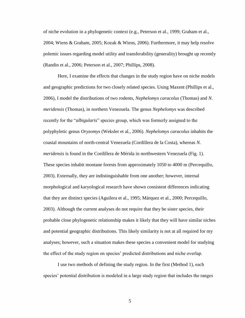
Here, I examine the effects that changes in the study region have on niche models
and geographic predictions for two closely related species. Using Maxent (Phillips et al.,
2006), I model the distributions of two rodents, Nephelomys caracolus (Thomas) and N.
meridensis (Thomas), in northern Venezuela. The genus Nephelomys was described
recently for the ―albigularis‖ species group, which was formerly assigned to the
polyphyletic genus Oryzomys (Weksler et al., 2006). Nephelomys caracolus inhabits the
coastal mountains of north-central Venezuela (Cordillera de la Costa), whereas N.
meridensis is found in the Cordillera de Mérida in northwestern Venezuela (Fig. 1).
These species inhabit montane forests from approximately 1050 to 4000 m (Percequillo,
2003). Externally, they are indistinguishable from one another; however, internal
morphological and karyological research have shown consistent differences indicating
that they are distinct species (Aguilera et al., 1995; Márquez et al., 2000; Percequillo,
2003). Although the current analyses do not require that they be sister species, their
probable close phylogenetic relationship makes it likely that they will have similar niches
and potential geographic distributions. This likely similarity is not at all required for my
analyses; however, such a situation makes these species a convenient model for studying
the effect of the study region on species‘ predicted distributions and niche overlap.
I use two methods of defining the study region. In the first (Method 1), each
species‘ potential distribution is modeled in a large study region that includes the ranges
Page 7
6
of both species. In the second (Method 2), each species is modeled in a smaller study
region immediately surrounding its known localities. The resulting model is then applied
(projected) to the larger region (that used for modeling in Method 1), identifying the
areas that are suitable for the species according to the model made using the smaller
study region. After making the models using each method, I analyze how well the
potential distribution of the focal species predicts the localities of the other species
(interpredictivity), indicating the level of niche conservatism (lack of niche evolution)
present between the species. Based on these results, I make recommendations for
selecting an appropriate study region.
Page 8
7
MATERIALS AND METHODS
Locality data
Niche-based distributional modeling requires two types of input data: known localities of
a species and environmental data for the study region. I obtained localities for the species
from a variety of taxonomic and faunal studies (Díaz de Pascual, 1994; Moscarella &
Aguilera, 1999; Márquez et al., 2000; Percequillo, 2003; Rivas & Salcedo, 2006). I then
georeferenced (assigned latitude and longitude to) each locality using gazetteers, detailed
topographic maps, and other sources (see Appendix 1), leading to 14 unique localities
(unique latitude–longitude combinations) for Nephelomys caracolus and 19 for N.
meridensis. The process of georeferencing includes an assessment of the uncertainties in
geographic coordinates (e.g., missing data, precision of the locality description, map
scale, and ambiguity in linear versus road distances). Based on the level of uncertainty, I
estimated maximum error in kilometers for the coordinates of each locality. Then, I
identified clusters of localities that likely represented the result of sampling bias (e.g.,
more sampling near major cities or universities, along roads, etc.). To reduce the effect of
sampling bias, I obtained the maximum number of localities for each species that were at
least 10 km apart (see below). When multiple equally optimal solutions were possible for
a given cluster, I retained the combination of localities with the lowest total error. This
process yielded 8 spatially filtered localities for N. caracolus and 8 for N. meridensis
(Fig. 1), which were used for all subsequent analyses. Although these filtered localities
are a reduced set, they have two important advantages over the original georeferenced
localities. First, since they likely reflect less of an environmental bias produced by
Page 9
8
uneven sampling by mammalogists, they should yield better estimates of the species‘
niches. Second, for the same reason, they provide more reasonable data for evaluating
how well the models of one species predict known localities of the other
(interpredictivity). Given the heterogeneity of the terrain in the known ranges of the
species, the cutoff of 10 km likely achieves these goals without unduly decreasing the
number of localities available for modeling.
Environmental variables
For the environmental data, I used 19 bioclimatic variables from WorldClim 1.4
(Hijmans et al., 2005; http://www.worldclim.org). These bioclimatic variables are derived
from monthly temperature and precipitation data to create variables that are more
biologically relevant (e.g., annual mean temperature, temperature of the wettest quarter,
precipitation seasonality, etc.; see Appendix 2). I used raster grids (data spatially
structured into grid cells, or pixels, each containing a value for a given variable) of these
bioclimatic variables with a spatial resolution of 30 seconds (0.93 km x 0.93 km = 0.86
km2 at the equator).
Defining the study region
As mentioned above, I used two methods of defining the study region in my analyses. In
Method 1 (Fig. 1A), following the practice typically used in the literature (see below), I
modeled the potential distribution of each species in a large study region that included the
ranges of both species as well as other adjacent regions of biogeographic interest
(extending the study region to the Caribbean coast in the north; 7.5–13º N and 65–72.5º
Page 10
9
W). In Method 2 (Fig. 1B, C), I modeled each species in a smaller study region
immediately surrounding its known, spatially filtered, localities (9.5–11º N and 66–69º W
for N. caracolus; 7.5–10º N and 69–72.5º W for N. meridensis). For Method 2, I then
applied the respective model to the larger study region (employed for modeling in
Method 1).
In delimiting the study regions in this way, I aimed to compare current common
practices in the field with a possible alternative. Most researchers delimit a study region
including all areas of interest to them when interpreting the model in geography (e.g.,
Kozak and Wiens 2006; Phillips et al., 2006). While Method 1 follows the spirit of this
common approach, Method 2 contrasts by being much smaller in most cases. An
alternative intermediate option could be to delimit a study region that immediately
encompasses only the areas surrounding both species‘ known occurrences. Here, such a
tactic would exclude the northernmost regions from 11–13º N (Fig. 1A). Because the
difference between such a study region and the one used for Method 1 in the current
study is only a difference of 2º in latitude (much of which falls in the Caribbean Sea), it is
likely that using such a study region would yield results similar to those obtained here. To
simplify comparisons, I only conducted experiments with two study regions but note that
the third option could be assessed in future analyses.
Each method has disadvantages in modeling a species‘ potential distribution.
When using a larger study region (Method 1) to model a species‘ niche, the model may
be prone to overfitting to environmental conditions present in the region where the
species is known to occur. Such a model would indicate that suitable regions for the
species are restricted to areas near known presences (overfitting due to bias in the
Page 11
10
localities used to generate the model). This can happen because the model recognizes
spurious environmental differences between the region that a species actually inhabits
versus other regions that it could inhabit but does not (e.g., because of a geographic
barrier that prevents it from dispersing to those regions). Overfitting leads to artificially
lowered transferability (Randin et al., 2006; see also Discussion).
However, when a model is constructed using a smaller study region (Method 2)
and then applied to a larger study region, the values for one or more environmental
variables in some pixels of the larger study region may not be covered by the niche model
(which is trained, in the smaller study region). This can arise because such values do not
occur in the study region used for training; hence, they lie outside the range of values for
the corresponding variable(s) in the study region used for making that niche model. This
arises in many other situations as well, such as when applying a model to another time
period (e.g., after climatic change) or region (e.g., prediction of an invasive species). In
these cases, some assumption about the potential suitability of those pixels must be made,
or no prediction can be generated for them (Phillips et al., 2006).
For example, at one extreme, all pixels holding values for climatic variables
outside the range (in environmental space) of those in the model can be assumed to be
unsuitable for the species; this almost certainly would lead to overly restrictive estimates
of a species‘ potential distribution. At the other end of the spectrum, such pixels could all
be assumed to be maximally suitable, producing an overly extensive estimate of the
species‘ potential distribution. Another possible assumption, intermediate between the
previous two, extrapolates the trend of environmental suitability that is modeled in the
training region. For example, if the model that is made in the smaller study region
Page 12
11
indicates that increasingly wetter environments are progressively more suitable for a
species, this assumption would lead to the prediction that environments wetter than those
found in the training region would be even better for the species. Extrapolation becomes
especially risky the farther that the pixel lies in environmental space from conditions
present in the training region, at least for response curves that are increasing when
truncated by the environment present in the training region.
Currently, Maxent resolves this issue via a more conservative assumption that is
termed ‗clamping‘ (similar in some ways to Winsorization in biostatistics; Sokal &
Rohlf, 1995). Under clamping, in cases where a pixel has a value for a given variable
outside the range covered in the model; that pixel is given the closest value present for
that variable in the model. For example, if the model calibrated in the smaller study
region indicates that increasingly wetter environments are progressively more suitable for
a species, the model would then predict that even wetter environments that are found in
the larger study region are equally good for the species (but not better). This is more
conservative, and probably more realistic, than extrapolation of the trend modeled in the
training region (see above). However, clamping remains an untested assumption in most
studies and will still be prone to erroneously extensive predictions for response curves
that are high (or increasing) when truncated by the environment present in the training
region. To alert the user to such possibilities, Maxent provides a map showing the degree
of clamping (if any) that was employed in each pixel when making a prediction into the
larger study region. No prediction should be interpreted without assessing the effect that
clamping has had on the prediction.
Page 13
12
Model building
I modeled the potential distributions of Nephelomys caracolus and N. meridensis using
Maxent version 3.1.0 (Phillips et al., 2006; Phillips & Dudík, 2008). Maxent has
performed well, based on quantitative measures of model performance, in recent
comparisons with other niche-based distributional modeling techniques (Elith et al.,
2006; Hernandez et al., 2006; Wisz et al., 2008). I used 19 bioclimatic variables and 8
localities for each species to make the models. I produced models using both linear and
quadratic features and with default levels of regularization (penalty for making a complex
model, thereby providing protection against overfitting). Lastly, I selected the logistic
output format, which yields continuous values ranging from 0–1 indicating relative
environmental suitability for the species (specifically, the probability of suitable
environmental conditions, or probability of presence if dispersal limitations or biotic
interactions are not relevant; see Phillips and Dudík, 2008). I first made preliminary
models to evaluate how well the models predicted localities of the focal species itself
(using some of the available spatially filtered localities; see below). The goal of these
preliminary models was to ensure that the variables used and model settings employed
can indeed produce satisfactory models for each individual species. These models were
assessed using threshold-dependent evaluations (see below). I then made final models for
each species using all available spatially filtered localities, which were used for all
subsequent analyses.
Page 14
13
Model evaluation
To evaluate the preliminary models, I used threshold-dependent evaluation as an
indicator of how well the model of each species predicted its own localities. Because only
8 localities of each species were available, I implemented the jackknife procedure for
model assessment (Pearson et al., 2007). For each species, 8 models were built by
removing each locality once in turn. In other words, a different set of 7 (out of 8)
localities was used to build the model during each training iteration (with a total of 8
iterations per species). Then, I assessed predictive performance based on the ability of
each model to predict the single locality excluded from the training data set. The
significance of the set of models for each species was assessed based on p-values
following Pearson et al. (2007). A p-value for the jackknife tests ≤ 0.05 indicates that test
localities are predicted better than by a random prediction with the same fractional
predicted area (fraction of the study area predicted suitable for a species). To divide the
continuous prediction into a binary prediction of presence or absence for these tests, I
used the minimum training weight (MTW) threshold (= lowest presence threshold of
Pearson et al., 2007). This is the minimum weight given to any of the training localities
and indicates the least-suitable environmental conditions for which a locality was
available in the training data set. I conducted these analyses for models made using the
smaller study region, and then for models produced using the larger study region.
Assessing interpredictivity
To compare the two methods of defining the study region, I used the final models to
assess interpredictivity between the species‘ niche models in three ways. First, I used the
Page 15
14
model for the focal species to assess the strength of the prediction of localities of the
other species by comparing the Area Under the Curve (AUC) of a Receiver Operating
Characteristic plot (Phillips et al., 2006) between the two methods. The AUC values
represent a threshold-independent measure of interpredictivity (independent of any cutoff
point dividing a prediction into suitable versus unsuitable areas for a species). Hence,
these cross-species AUC values provide an overall assessment of how well the model of
each focal species predicted localities of the other. For models made using Method 1, I
was able to obtain cross-species AUC values from Maxent by specifying the localities for
that species as test localities in the focal species‘ model. However, this was not possible
for models built using Method 2. Therefore, for Method 2, I obtained cross-species AUC
using DIVA-GIS 5.2 (Hijmans et al., 2001; http://www.diva-gis.org). For each species, I
selected 1500 random background pixels from the larger study region, along with the
pixels corresponding to the localities of the test species, which together were used to
obtain ROC plots and the cross-species AUC values for Method 2.
The second way I assessed interpredictivity was by calculating cross-species
omission rates, a threshold-dependent measure that indicates how well the model of the
focal species predicts localities of the other species. We applied a threshold to convert the
continuous prediction of environmental suitability for the species (logistic values from 0
to 1) into a binary prediction, dividing the study region into areas predicted suitable
versus unsuitable for the species. As in assessing the preliminary models, I achieved this
by applying the minimum training weight (MTW) threshold. Using this binary prediction,
I calculated the cross-species omission rates by determining the percentage of localities
of the other species falling outside of (omitted from) areas predicted suitable for the focal
Page 16
15
species. I then compared these between the two methods.
Third, I examined the effect that the two methods have on the degree of
geographic overlap between the two species‘ potential distributions. I accomplished this
by superimposing the potential distributions of the two species in the larger study region
(after applying the MTW threshold rule; see above). Then, the percentage of geographic
overlap was estimated by dividing the number of pixels predicted suitable for both
species by (1) the total number of pixels with data (e.g., excluding the ocean), (2) the
total number of pixels predicted suitable for each species alone, and (3) the total number
of pixels predicted suitable for either species.
Predictions
I expected the predicted species‘ distributional models to be less concentrated in the
region surrounding the species‘ localities in Method 2 (reduced overfitting; likely a
problem for Method 1). Therefore, I predicted higher interpredictivity in Method 2, as
evaluated by (1) higher cross-species AUC values, (2) lower cross-species omission rates,
and (3) higher percentage of geographic overlap.
Page 17
16
RESULTS
Preliminary models
Threshold-dependent evaluation via the jackknife procedure revealed that the models
adequately predicted each individual species‘ potential distribution. Pixels with values
greater than or equal to the MTW threshold are considered suitable, whereas pixels with
values below that threshold are deemed unsuitable. Test omission rates were low (≤ 25%;
only 1 of 8 iterations omitted the test locality, except for Method 2 for N. caracolus in
which 2 of 8 iterations omitted the test locality). Furthermore, the jackknife tests
indicated that the models were significantly better than random predictions for both
species, with p-values well below 0.05 (p ≤ 1 x 10⁻⁶
). Omission rates and significance
values were similar for models made with the two study regions.
Qualitative assessment of final models
Maxent generated models of the potential distribution of each species showing a
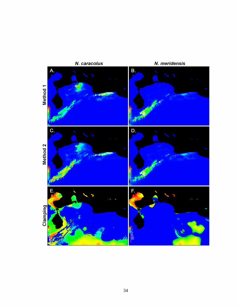
continuous prediction of relative suitability (Fig. 2A–D). The prediction for Nephelomys
caracolus revealed highest suitability in the mountain ranges of the north-central coast,
the Cordillera de Mérida (northwestern Venezuela), and the Serrenía de San Luis
(northwestern coast of Venezuela), separated by gaps of low suitability between these
ranges (Fig. 2A, C). In contrast, the areas strongly predicted for N. meridensis generally
appeared to be restricted to the Cordillera de Mérida (Fig. 2B, D). The models for each
species varied depending on the method of defining the study region. Models generated
using Method 2 predicted larger areas with high suitability than models generated using
Page 18
17
Method 1. Additionally, Method 1 yielded models with the highest suitability generally
restricted to areas near the focal species‘ known localities, whereas Method 2 produced
predictions that were less concentrated around the known localities of the focal species.
Clamping was minimal in most of the study region. In the present analyses, areas
with a high degree of clamping occurred primarily in lowland regions that are unlikely to
be suitable for the species (Fig. 2E, F). These included extremely dry lowland regions in
the Península de la Guajira in northeastern Colombia and northwestern Venezuela, and
along the Caribbean coast of northwestern Venezuela, both east and west of the mouth of
the Lago de Maracaibo. Another area of high clamping occurred in very wet regions at
the base of the Cordillera de Mérida, southwest of the Lago de Maracaibo.
Quantitative assessment of interpredictivity
Cross-species AUC values varied between the two methods of defining the study region.
The AUC for the localities of Nephelomys meridensis in the predicted potential
distribution of N. caracolus was slightly higher in Method 2 (Table 1). Similarly, the
potential distribution of N. meridensis predicted the known localities of N. caracolus with
a slightly higher AUC in Method 2 (Table 1).
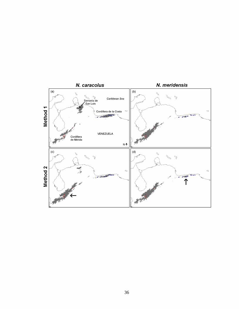
Cross-species omission rates were lower in models made using Method 2
compared with Method 1. Models of Nephelomys caracolus predicted localities of N.
meridensis better than models of N. meridensis predicted localities of N. caracolus. At
the MTW threshold, the potential distribution of N. caracolus predicted slightly over half
of the known localities of N. meridensis using Method 1, but achieved an omission rate of
zero using Method 2 (Fig. 3A, C; Table 1). In contrast, the potential distribution of N.
Page 19
18
meridensis predicted only half of the known localities of N. caracolus in Method 1, and
slightly more in Method 2 (Fig. 3B, D; Table 1; at MTW threshold).
The two species showed substantial yet incomplete geographic overlap, but those
estimates varied depending on the method of defining the study region. Method 2
revealed a larger predicted area for each species compared with Method 1 (Fig. 3). Not
surprisingly, percentages of geographic overlap between the two species‘ predicted
distributions were consistently higher using Method 2 (Table 2).
Page 20
19
DISCUSSION
My results show differences in the predicted potential distributions and in estimates of
interpredictivity between the two methods of defining the study region. Method 2 appears
to perform better because it reduces overfitting (a problem observed for Method 1).
Clamping (a possible drawback to Method 2) did not seem to be a problem in the models
analyzed here. These results suggest that the study region used for modeling a species‘
potential distribution should not include areas where the species may be absent due to
dispersal limitation. This is because background pixels randomly drawn from suitable
environments in such regions provide a false negative signal that interferes with
successful modeling of the species‘ environmental requirements. Similarly, I also propose
that the study region for modeling should not include areas where biotic interactions with
other species (principally competition) are likely to restrict the species‘ distribution to
less than its potential (Anderson et al., 2002), for the same reasons mentioned for
dispersal limitation. Clearly, such information will be difficult to estimate in many cases.
Future research should aim to develop operational guidelines for selecting an appropriate
study region based on these principles.
Recent studies have used niche modeling to investigate evolutionary processes,
and studies that follow this line of research should consider definition of the extent of the
study region and background selection carefully. Niche conservatism refers to the
propensity for species to maintain the same niche over evolutionary time (Peterson et. al.,
1999). Building on these concepts, Graham et al. (2004) proposed ways to study
speciation by integrating phylogenetic information, distributional overlap of species, and
Page 21
20
niche models. Similarly, Kozak and Wiens (2006) suggested that niche conservatism and
climatic differences in geographic space could play an important role in speciation
events. To conduct valid tests of hypotheses of niche evolution versus niche
conservatism, researchers should select an appropriate study region for making niche-
based models in order to obtain the best estimates of niche overlap.
Additionally, my results are relevant to other areas of research using niche-based
distribution modeling. Any application requiring an estimate of the species‘ potential
geographic distribution should strive to conduct modeling based on an appropriate study
region. In particular, selection of an appropriate study region is especially germane for
studies of invasive species and of species‘ distributional changes under climatic change
(Welk et al., 2002; Araújo et al., 2005). In both of those applications, model
transferability (or generality) is critical (Araújo & Rahbek, 2006; Randin et al., 2006;
Peterson et al., 2007; Phillips, 2008). Transferability refers to how adequately a model
produced in one situation may be transferred to a different context to provide useful
insight in the latter case (e.g., another time period after climatic change; or another region
in the prediction of an invasive species). Whereas models produced with an overly large
study region likely will show low transferability, models made based on an appropriate
study region should show higher transferability. The conceptual advances and principles
espoused here also may help resolve some currently controversial issues regarding
characterization of the background (the study region) and its association to the region
from which the training localities derive (Peterson et al., 2007; Phillips, 2008);
specifically, future research should consider the possibility that selecting training records
from only some portions of the study region may mimic the natural processes discussed
Page 22
21
here (dispersal limitation and biotic interactions) that can cause a species to inhabit less
than its potential distribution.
Page 23
22
ACKNOWLEDGMENTS
The current research was possible via funding from the U.S. National Science Foundation
(NSF DEB-0717357, to RPA); American Society of Mammalogists (ASM Undergraduate
Student Research Award, to AR); and City College Academy for Professional
Preparation (CCAPP, support to AR) and Office of the Dean of Science and Office of the
Provost (City College of New York, City University of New York). I thank Robert P.
Anderson for his helpful advice and great mentorship, and for his continuous help in
completing the thesis. Thanks go to Eliécer E. Gutierrez and Mariya Shcheglovitova for
their assistance in data collection, and to Eliécer E. Gutierrez, Aleksandar Radosavljevic,
Darla M. Thomas, and the New York Species Distribution Modeling Discussion Group
for comments and suggestions. Finally, I thank Amy C. Berkov and David J. Lohman for
being on the committee and for their helpful comments.
Page 24
23
REFERENCES
Aguilera, M., Pérez-Zapata, A. & Martino, A. (1995) Cytogenetics and karyosystematics
of Oryzomys albigularis (Rodentia, Cricetidae) from Venezuela. Cytogenetics and
Cell Genetics, 69, 44–49.
Anderson, R.P. (2003) Real vs. artefactual absences in species distributions: tests for
Oryzomys albigularis (Rodentia: Muridae) in Venezuela. Journal of
Biogeography, 30, 591–605.
Anderson, R.P., Peterson, A.T. & Gómez-Laverde, M. (2002) Using niche-based GIS
modeling to test geographic predictions of competitive exclusion and competitive
release in South American pocket mice. Oikos, 98, 3–16.
Araújo, M.B. & Rahbek, C. (2006) How does climate change affect biodiversity?
Science, 313, 1396–1397.
Araújo, M.B., Pearson, R.G., Thuiller, W. & Erhard, M. (2005) Validation of species–
climate impact models under climate change. Global Change Biology, 11,1504–
1513.
DCN. (1964) Hoja 6847 (Caracas), escala 1:100.000. Dirección de Cartografía Nacional,
Ministerio de Obras Públicas, Caracas.
DCN. (1975) Hoja 5941-I-NE (Tabay), escala 1:25.000. Dirección de Cartografía
Nacional, Ministerio de Obras Públicas, Caracas.
DCN. (1977a) Hoja 5941 (Mérida), escala 1:100.000. Dirección de Cartografía Nacional,
Ministerio del Ambiente y de los Recursos Naturales Renovables, Caracas.
DCN. (1977b) Hoja 5942 (La Azulita), escala 1:100.000. Dirección de Cartografía
Page 25
24
Nacional, Ministerio del Ambiente y de los Recursos Naturales Renovables,
Caracas.
DCN. (1979a) Hoja 6847-I-SE (Perque), escala 1:25.000. Dirección de Cartografía
Nacional, Ministerio del Ambiente y de los Recursos Naturales Renovables,
Caracas.
DCN. (1979b) Hoja 6847-IV-SE (Los Chorros), escala 1:25.000. Dirección de
Cartografía Nacional, Ministerio del Ambiente y de los Recursos Naturales
Renovables, Caracas.
Díaz de Pascual, A. (1994) The rodent community of the Venezuelan cloud forest,
Mérida. Polish Ecological Studies, 20, 155–161.
Elith, J., Graham, C.H., Anderson, R.P., Dudík, M., Ferrier, S., Guisan, A., Hijmans, R.J.,
Huettmann, F., Leathwick, J.R., Leahmann., A., Li, J., Lohmann, L.G., Loiselle,
B.A., Manion, G., Moritz, C., Nakamura, M., Nakazawa, Y., Overton, J.M.,
Peterson, A.T., Phillips, S.J., Richardson, K., Scachetti-Pereira, R., Schapire,
R.E., Soberón, J., Williams, S., Wisz, M.S. & Zimmermann, N.E. (2006) Novel
methods improve prediction of species‘ distributions from occurrence data.
Ecography, 29, 129–151.
Graham, C.H., Ferrier, S., Huettman, F., Moritz, C. & Peterson, A.T. (2004) New
developments in museum-based informatics and application in biodiversity
analysis. Trends in Ecology and Evolution, 19, 497–503.
Graham, C.H., Ron, S.R., Santos, J.C., Schneider, C.J. & Moritz, C. (2004) Integrating
phylogenetics and environmental niche models to explore speciation mechanisms
in dendrobatid frogs. Evolution, 58, 1781–1793.
Page 26
25
Handley, C.O., Jr. (1976) Mammals of the SmithsonianVenezuelan Project. Brigham
Young University Science Bulletin, Biological Series, 20(5), 1–91.
Hernandez, P.A., Graham, C.H., Master, L.L. & Albert, D.L. (2006) The effect of sample
size and species characteristics on performance of different species distribution
modeling methods. Ecography, 29, 773–785.
Hijmans, R.J., Guarino, L., Cruz, M. & Rojas, E.. (2001) Computer tools for spatial
analysis of plant genetic resources data: 1. DIVA-GIS. Plant Genetic Resources
Newsletter, 127, 15–19.
Hijmans, R.J., Cameron, S.E., Parra, J.L., Jones, P.G. & Jarvis, A. (2005) Very high
resolution interpolated climate surfaces for global land areas. International
Journal of Climatology, 25, 1965–1978.
Kozak, K.H. & Wiens, J.J. (2006) Does niche conservatism promote speciation? A case
study in North American salamanders. Evolution, 60, 2604–2621.
Kremen, C., Cameron, A., Moilanen, A., Phillips, S.J., Thomas, C.D., Beentje, H.,
Dransfield, J., Fisher, B.L., Glaw, F., Good, T.C., Harper, G.J., Hijmans, R.J.,
Lees, D.C., Louis, Jr., E., Nussbaum, R.A., Raxworthy, C.J., Razafimpahanana,
A., Schatz, G.E., Vences, M., Vieites, D.R., Wright, P.C. & Zjhra, M.L. (2008)
Aligning conservation priorities across taxa in Madagascar with high-resolution
planning tools. Science, 320, 222–226.
Márquez, E.J., Aguilera-M., M. & Corti, M. (2000) Morphometric and chromosomal
variation in populations of Oryzomys albigularis (Muridae: Sigmodontinae) from
Venezuela: multivariate aspects. Zeitschrift für Säugetierkunde, 65, 84–99.
Moscarella, R.A. & Aguilera-M., M. (1999) Growth and reproduction of Oryzomys
Page 27
26
albigularis (Muridae: Sigmodontinae) under laboratory conditions. Mammalia,
63, 349–362.
Paynter, R.A., Jr. (1982) Ornithological gazetteer of Venezuela. Museum of Comparative
Zoology, Harvard University, Cambridge, MA.
Pearson, R.G., Raxworthy, C.J., Nakamura, M. & Peterson, A.T. (2007) Predicting
species distributions from small numbers of occurrence records: a test case using
cryptic geckos in Madagascar. Journal of Biogeography, 34, 102–117.
Percequillo, A.R. (2003) Sistemática de Oryzomys Baird, 1858: definição dos grupos de
espécie e revisão taxonômica do grupo albigularis (Rodentia, Sigmodontinae),
Ph.D. Thesis. Universidade de São Paulo, Brazil.
Peterson, A.T., Soberón, J. & Sánchez-Cordero, V. (1999) Conservatism of ecological
niches in evolutionary time. Science, 285, 1265–1267.
Peterson, A.T., Papeş, M. & Eaton, M. (2007) Transferability and model evaluation in
ecological niche modeling: a comparison of GARP and Maxent. Ecography, 30,
550–560.
Phelps, W.H. (1944) Resumen de las colecciones ornitológicas hechas en Venezuela.
Boletín de la Sociedad Venezolana de Ciencias Naturales, 61, 325–444.
Phillips, S.J. (2008) Transferability, sample selection bias and background data in
presence-only modelling: a response to Peterson et al. (2007). Ecography, 31,
272–278.
Phillips, S.J. & Dudík, M. (2008) Modeling of species distributions with Maxent: new
extensions and a comprehensive evaluation. Ecography, 31, 161–175.
Phillips, S.J., Anderson, R.P. & Schapire, R.E. (2006) Maximum entropy modeling of
Page 28
27
species geographic distributions. Ecological Modelling, 190, 231–259.
Randin, C.F., Dirnböck, T., Dullinger, S., Zimmermann, N.E., Zappa, M. & Guisan, A.
(2006) Are niche-based species distribution models transferable in space? Journal
of Biogeography, 33, 1689–1703.
Rivas, B.A. & Salcedo, M.A. (2006) Lista actualizada de los mamíferos del Parque
Nacional El Ávila, Venezuela. Memorias de la Fundación La Salle de Ciencias
Naturales, 164, 29–56.
Sokal, R.R. & Rohlf, F.J. (1995) Biometry: the principles and practice of statistics in
biological research, 3rd edn. W. H. Freeman, New York.
Weksler, M., Percequillo, A.R. & Voss, R.S. (2006) Ten new genera of oryzomyine
rodents (Cricetidae: Sigmodontinae). American Museum Novitates, 3537, 1–29.
Welk, E., Schubert, K. & Hoffmann, M.H. (2002) Present and potential distribution of
invasive garlic mustard (Alliaria petiolata) in North America. Diversity and
Distributions, 8, 219–233.
Wiens, J.J. & Graham, C.H. (2005) Niche conservatism: integrating evolution, ecology,
and conservation biology. Annual Review of Ecology and Systematics, 36, 519–
539.
Wisz, M.S., Hijmans, R.J., Li, J., Peterson, A.T., Graham, C.H. & Guisan, A. (2008)
Effects of sample size on the performance of species distribution models.
Diversity and Distributions, 14, 763–773.
Zaniewski, A.E., Lehmann, A. & Overton, J.M. (2002) Predicting species spatial
distributions using presence-only data: a case study of native New Zealand ferns.
Ecological Modelling, 157, 261–280.
Page 29
28
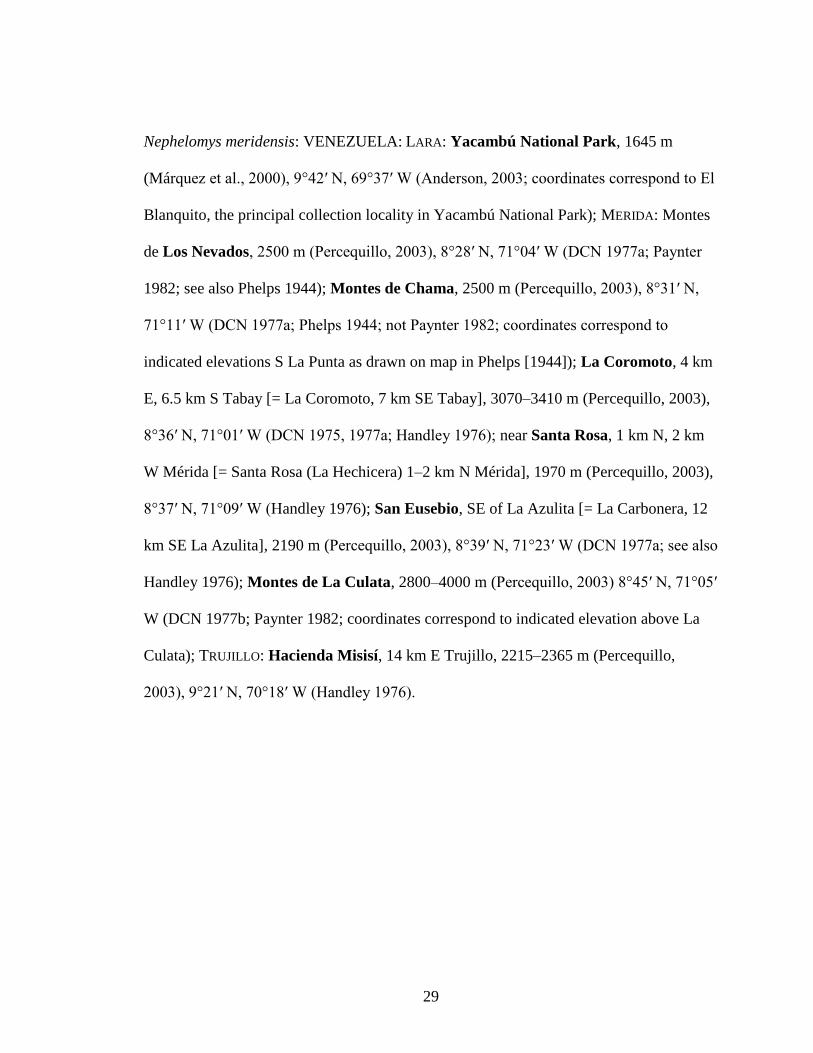
Appendix 1. Gazetteer of spatially filtered occurrence records used in this study.
Boldface type indicates the place to which geographic coordinates correspond. The
source for the record follows the elevation, and the source for the coordinates follows the
latitude and longitude.
Nephelomys caracolus: VENEZUELA: ARAGUA: Rancho Grande, Estación Biológica
de Rancho Grande, 13 km NW Maracay [= 14 km N, 14 km W Maracay, Rancho
Grande], 1050–1100 m (Percequillo, 2003), 10°21′ N, 67°40′ W (Handley 1976);
Natural Monument Pico Codazzi, Coastal Cordillera, 1700 m (Moscarella & Aguilera
1999), 10°23′ N, 67°20′ W (Moscarella & Aguilera 1999); CARABOBO: La Cumbre de
Valencia, 1700 m (Percequillo, 2003), 10°20′ N, 68°00′ W (Paynter 1982); DISTRITO
CAPITAL: Los Venados, 4 km NNW Caracas [= 5 mi N Caracas], 1400–1739 m
(Percequillo, 2003), 10°32′ N, 66°54′ W (Handley 1976); DISTRITO
CAPITAL/MIRANDA/VARGAS: Alto Ño León, 31–36 km WSW Caracas [= 5 km S, 23 km
W Caracas, Alto Ño León; Alto Ño León, 20 km W Caracas; Petaquire, 20 km N (W)
Caracas], 1665–2050 m (Percequillo, 2003), 10°26′ N, 67°10′ W (Handley 1976);
MIRANDA: 5 km NNW Guarenas [= Curupao, 19 km E Caracas], 1160 m (Percequillo,
2003), 10°31′ N, 66°38′ W (Handley 1976); Quebrada Caurimare, Fila Santa Rosa,
Parque Nacional El Ávila, 1750 m (Rivas & Salcedo, 2006), 10°31′ N, 66°47′ W (DCN
1964, 1979b; coordinates correspond to Río Caurimare [= Quebrada Caurimare] at
indicated elevation); Hacienda Las Planadas, aproximadamente 25 km [by road] N de
Guatire, 1270 m (Rivas & Salcedo, 2006), 10°32′ N, 66°30′ W (DCN 1964, 1979a;
coordinates correspond to indicated elevation at Hacianda Las Planadas).
Page 30
29
Nephelomys meridensis: VENEZUELA: LARA: Yacambú National Park, 1645 m
(Márquez et al., 2000), 9°42′ N, 69°37′ W (Anderson, 2003; coordinates correspond to El
Blanquito, the principal collection locality in Yacambú National Park); MERIDA: Montes
de Los Nevados, 2500 m (Percequillo, 2003), 8°28′ N, 71°04′ W (DCN 1977a; Paynter
1982; see also Phelps 1944); Montes de Chama, 2500 m (Percequillo, 2003), 8°31′ N,
71°11′ W (DCN 1977a; Phelps 1944; not Paynter 1982; coordinates correspond to
indicated elevations S La Punta as drawn on map in Phelps [1944]); La Coromoto, 4 km
E, 6.5 km S Tabay [= La Coromoto, 7 km SE Tabay], 3070–3410 m (Percequillo, 2003),
8°36′ N, 71°01′ W (DCN 1975, 1977a; Handley 1976); near Santa Rosa, 1 km N, 2 km
W Mérida [= Santa Rosa (La Hechicera) 1–2 km N Mérida], 1970 m (Percequillo, 2003),
8°37′ N, 71°09′ W (Handley 1976); San Eusebio, SE of La Azulita [= La Carbonera, 12
km SE La Azulita], 2190 m (Percequillo, 2003), 8°39′ N, 71°23′ W (DCN 1977a; see also
Handley 1976); Montes de La Culata, 2800–4000 m (Percequillo, 2003) 8°45′ N, 71°05′
W (DCN 1977b; Paynter 1982; coordinates correspond to indicated elevation above La
Culata); TRUJILLO: Hacienda Misisí, 14 km E Trujillo, 2215–2365 m (Percequillo,
2003), 9°21′ N, 70°18′ W (Handley 1976).
Page 31
30
Appendix 2. List of the 19 bioclimatic variables from WorldClim 1.4 (Hijmans et al.,
2005; http://www.worldclim.org) that were used in this study.
1. Annual mean temperature
2. Mean diurnal range (mean of monthly values of maximum temperature minus
minimum temperature)
3. Isothermality
4. Temperature seasonality
5. Maximum temperature of the warmest month
6. Minimum temperature of the coldest month
7. Temperature annual range
8. Mean temperature of the wettest quarter
9. Mean temperature of the driest quarter
10. Mean temperature of the warmest quarter
11. Mean temperature of the coldest quarter
12. Annual precipitation
13. Precipitation of the wettest month
14. Precipitation of the driest month
15. Precipitation seasonality
16. Precipitation of the wettest quarter
17. Precipitation of the driest quarter
18. Precipitation of the warmest quarter
19. Precipitation of the coldest quarter
Page 32
31
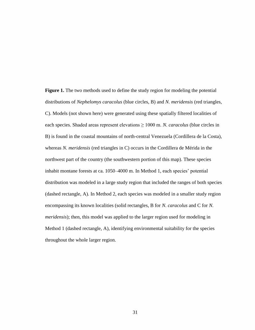
Figure 1. The two methods used to define the study region for modeling the potential
distributions of Nephelomys caracolus (blue circles, B) and N. meridensis (red triangles,
C). Models (not shown here) were generated using these spatially filtered localities of
each species. Shaded areas represent elevations ≥ 1000 m. N. caracolus (blue circles in
B) is found in the coastal mountains of north-central Venezuela (Cordillera de la Costa),
whereas N. meridensis (red triangles in C) occurs in the Cordillera de Mérida in the
northwest part of the country (the southwestern portion of this map). These species
inhabit montane forests at ca. 1050–4000 m. In Method 1, each species‘ potential
distribution was modeled in a large study region that included the ranges of both species
(dashed rectangle, A). In Method 2, each species was modeled in a smaller study region
encompassing its known localities (solid rectangles, B for N. caracolus and C for N.
meridensis); then, this model was applied to the larger region used for modeling in
Method 1 (dashed rectangle, A), identifying environmental suitability for the species
throughout the whole larger region.
Page 34
33
Figure 2. Models of the potential geographic distributions of Nephelomys caracolus (left)
and N. meridensis (right), for each method of defining the study region. The predictions
(A–D) show a suitability gradient from low (blue = 0) to high (red = 1) relative
environmental suitability. White squares indicate the localities used to make the models.
Panels A and B show predictions generated using Method 1 (models made using the large
study region), while C and D correspond to the respective predictions for Method 2
(models made using the smaller study region and then projected to the larger one). For
Method 2 for each species, E and F reveal the level of clamping, if any, corresponding to
each map pixel. Clamping occurs when values of environmental variables fall outside of
the range of environmental values in the models (see text). Successively warmer colors
show areas where the strength of clamping was greater.
Page 36
35
Figure 3. Models of the potential distributions of Nephelomys caracolus (A, C) and N.
meridensis (B, D), for each method of defining the study region, showing binary
predictions of the extent of suitable conditions for each species after applying the
minimum training weight (MTW) threshold. Each prediction is divided into areas
considered suitable (grey) vs. unsuitable (white) for the species. Blue circles and red
triangles indicate localities for N. caracolus and N. meridensis, respectively. Panels A
and B indicate predictions made using Method 1 (models made using the large study
region), while C and D illustrate the corresponding predictions for Method 2 (models
made using the smaller study region and then applied to the larger one). Note the much
larger prediction for N. caracolus in the Cordillera de Mérida under Method 2 (arrow in
C). In contrast, the prediction for N. meridensis in the Cordillera de la Costa is only
slightly larger under Method 2 (arrow in D).
Page 38
37
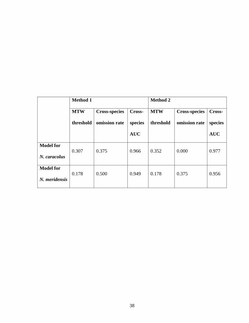
Table 1. Measures of interpredictivity between Nephelomys caracolus and N. meridensis
based on models made with two different methods of defining the study region. In
Method 1, each species‘ potential distribution was modeled in a large study region that
included the range of both species (left). In Method 2, each species was modeled in a
smaller study region encompassing its known localities, and then applied (projected) to
the larger study region (right). Both cross-species omission rates and cross-species AUC
values provide measures of how well the model of the focal species predicts localities of
the other species. Omission rates constitute a threshold-dependent measure: first, the
minimum training weight (MTW) threshold rule is applied to the model of the focal
species, yielding a binary prediction; then, the omission rate for localities of the other
species is calculated. Complementarily, AUC values represent a threshold-independent
measure that assesses the overall ability (across all possible thresholds) of the model for
the focal species to predict localities of the other species. Low omission rates and high
AUC values indicate high interpredictivity (and low levels of niche evolution). Note that
both measures indicate higher interpredictivity for Method 2. The MTW threshold values
are provided as additional information regarding the models, but they do not address the
issue of interpredictivity. See text for further discussion of omission rates.
Page 39
38
Method 1 Method 2
MTW
threshold
Cross-species
omission rate
Cross-
species
AUC
MTW
threshold
Cross-species
omission rate
Cross-
species
AUC
Model for
N. caracolus
0.307 0.375 0.966 0.352 0.000 0.977
Model for
N. meridensis
0.178 0.500 0.949 0.178 0.375 0.956
Page 40
39
Table 2. Measures of percent geographic overlap of the potential distributions of
Nephelomys caracolus and N. meridensis, for each method of defining the study region.
In Method 1, each species‘ potential distribution was modeled in a large study region that
included the range of both species. In Method 2, each species was modeled in a smaller
study region encompassing its known localities, and then applied (projected) to the larger
study region. All results are for predictions of the species‘ potential distributions in the
larger study region (even though the models for Method 2 were made in the smaller study
region), and after converting the continuous prediction to a binary one based on the
minimum training weight (MTW) threshold (see text). The percent geographic overlap
was calculated in three ways based on overlap of the two species‘ predictions as a
percentage of: (1) the larger study region; (2) the prediction for each respective species
alone; and (3) the area predicted for either species. The last measure provides the best
single indicator of the amount of geographic overlap between the predictions of the two
species.
Page 41
40
Percent geographic overlap based on number of pixels in: Method 1 Method 2
overlap relative to larger study region 1.8 3.4
overlap relative to prediction of N. caracolus 50.1 74.7
overlap relative to prediction of N. meridensis 47.0 84.9
overlap relative to prediction of either species 32.0 65.9