The Effectiveness of Homeownership in Building Household ...

The Effectiveness of Homeownership in Building Household Wealth

By Jordan Rappaport

The recent economic and financial crisis and the current slow recovery highlight that homeownership plays a critical role in the U.S. economy. The estimated “equivalent rent” implicitly

paid by homeowners accounts for more than 8 percent of gross domes-tic product (GDP). Investment in single-family housing also represents a significant share of GDP and is closely tied to the business cycle. Over the past decade, such investment has ranged from as little as 1.3 percent of GDP during recessions to as much as 3.4 percent during expansions. The associated large fluctuations in demand for owner-occupied housing play an important role in driving the business cycle. In addition, demand for owner-occupied housing is especially sensitive to intermediate-term real interest rates and hence to inflation and mon-etary policy expectations.

Homeownership also plays an important role in determining household saving, which has implications for national saving and in-vestment. Some aspects of homeownership increase household and na-tional saving. For example, renters intending to purchase a home have an incentive to save to make a down payment on their first home. In

Jordan Rappaport is a senior economist at the Federal Reserve Bank of Kansas City. Li Yi, a research associate at the bank, helped prepare the article. The author would like to thank Daniel Feenberg of the National Bureau of Economic Research for invaluable assistance. This article is on the bank’s website at www.KansasCityFed.org.

35

36 FEDERAL RESERVE BANK OF KANSAS CITY

addition, new homeowners must promise to save far into the future by making monthly mortgage principal payments. On the other hand, homeownership typically requires large house-related payments and so can reduce household cash flows available to invest in financial assets such as stocks and bonds.

For decades, conventional wisdom has viewed homeownership as an effective way to build household wealth. However, the recent fall in house prices has caused some observers to question this belief. This article examines whether homeownership effectively builds household wealth. It develops an analytical framework to compare the wealth that homeowners have historically accumulated by building equity in their houses with the wealth they could have accumulated by renting an identical house and investing the resulting saved cash flow in stocks and bonds.

The first section describes the analytical framework. The second sec-tion uses the framework to compare building wealth by owning and by renting an identical house for ten-year occupancies beginning in 1970 through 1999. The article finds that for ten-year occupancies beginning during most of the 1970s and 1990s, homeowners built more wealth than renters. In contrast, for ten-year occupancies beginning during most of the 1980s, renters who invested their savings from lower house payments (than owners) built more wealth. For other periods (about a quarter of the ten year occupancies), it is unclear whether owning or renting built more wealth. This ambiguity arises from the difficulty of measuring the market rent and purchase price on identical houses.

I. ANALYTICAL FRAMEWORK

Comparing the wealth built by purchasing and building equity in a house with the wealth built by renting an identical house and invest-ing any saved cash flow in stocks and bonds requires a framework that tracks the many cash flows associated with owning and renting. These flows include both one-time items, such as making a down payment on a house, and recurring payments, such as monthly mortgage and rent payments. Such a focus on cash flows is needed because the many costs, investments, transfers and taxes associated with owning and renting a house are together too complicated to allow a simpler comparison of net present values.1

ECONOMIC REVIEW • FOURTH QUARTER 2010 37

This section details the framework for this flow accounting—spe-cifically, the framework for taking account of the many cash flows that affect the wealth accumulation of owners and renters. In particular, it describes the cash and financial flows associated with owning and rent-ing a house, the saved cash flow that the renter can invest in stocks and bonds, the breakeven rent-to-price ratio at which owners and renters accumulate equal wealth, and the market rent-to-price ratio at which households can rent or purchase an identical house. Ultimately, the article’s assessment of the merits of ownership and renting for wealth accumulation will rest on the comparison of the breakeven and market rent-to-price ratios.

Cash and financial flows associated with homeownership and renting

The analytical framework for comparing the wealth built from homeownership and renting is based on tracking the wealth accumula-tion of two hypothetical households with identical composition and equal labor income. One household purchases a house, while the oth-er rents an identical house.2 Over the course of ten-year occupancies, the owner household makes numerous house-related payments, and the renter household makes monthly rent payments.3 In addition, the renter regularly makes new investments in stocks and bonds. The two households are assumed to spend an equal amount on non-housing consumption. As a result, the amount the renter splits between paying rent and investing in stocks and bonds exactly equals the total of all homeowner payments.4 At the end of ten years, the owner household sells its house and the renter household liquidates its stock and bond portfolio.

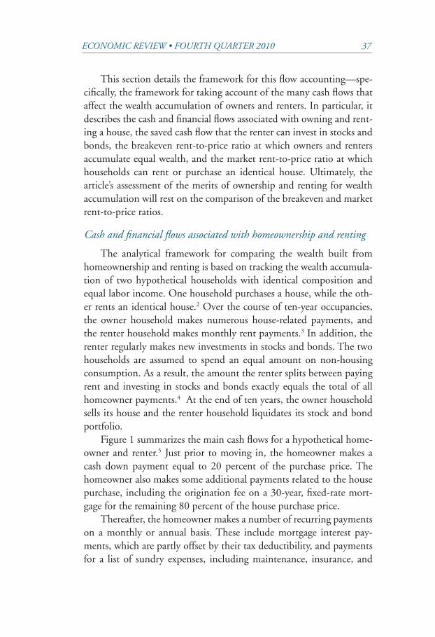
Figure 1 summarizes the main cash flows for a hypothetical home-owner and renter.5 Just prior to moving in, the homeowner makes a cash down payment equal to 20 percent of the purchase price. The homeowner also makes some additional payments related to the house purchase, including the origination fee on a 30-year, fixed-rate mort-gage for the remaining 80 percent of the house purchase price.

Thereafter, the homeowner makes a number of recurring payments on a monthly or annual basis. These include mortgage interest pay-ments, which are partly offset by their tax deductibility, and payments for a list of sundry expenses, including maintenance, insurance, and


real estate taxes. In addition, the homeowner makes monthly mortgage principal payments, which build home equity. At the end of ten years, the owner sells his house, pays the associated selling costs, and pays off the outstanding mortgage balance. The remaining cash constitutes the owner’s final wealth.

Just prior to moving in, the renter is assumed to make an initial investment in stocks and bonds equal to the owner’s down payment plus other purchase costs. This matching of the owner’s and the renter’s initial payments reflects a more general requirement that, at any point in time, the renter’s payments on rent and investment must equal the homeowner’s payments on housing. As a result of this matching, any difference in final wealth between the owner and renter reflects the rel-ative effectiveness of homeownership and renting in building wealth rather than differences in the nonhousing consumption of the home-owner and renter.

During each of the ten years of occupancy, the renter pays an annual rent, which increases at the national rate of rent inflation. The renter also makes new investments in stocks and bonds. The annual sum of

Figure 1

invest in stocks + bonds

rent

new investment

sell stocks + bonds, pay taxes

portfolio wealth

home equity

down payment

start years 1-10

Final Wealth

mortgage interest less tax savings,

maintenance, other owner

payments end

year 10

renter owner

cash cash

selling price less mortgage balance less selling costs

mortgage principal payments

other purchase payments


rent and new investments equals the sum of the homeowner’s annual payments. At the end of ten years, the renter liquidates his stock and bond portfolio and pays any taxes due. The remainder constitutes the renter’s final wealth.

Renter saved cash flow

Typically, annual homeownership payments considerably exceed annual rent. It is helpful to think of this excess as “saved” cash flow that the renter does not have to spend on housing. The renter is assumed to invest all saved cash flow in stocks and bonds. In other words, he does not use any saved cash flow to increase his nonhousing consump-tion. As an accounting identity, saved cash flow equals homeowner payments less rent. Thus, any increase in rent (holding homeowner payments constant) implies that saved cash flow and hence renter new investment must fall by an offsetting amount. As a result, the renter’s final wealth also falls. Conversely, any increase in the homeowner’s pay-ments (holding rent constant) implies higher saved cash flow and hence higher renter new investment. As a result, the renter’s final wealth also increases.

Breakeven rent-to-price ratio

A key concept in the analysis is the breakeven rent-to-price ratio. This is simply the rent at the beginning of an occupancy for a given house purchase price that equalizes the owner’s and the renter’s final wealth. A low breakeven ratio indicates that homeownership is likely to be the more effective means of building wealth, and a high ratio indi-cates that renting is likely to be more effective.

To match a given final wealth of the homeowner, the renter must have a certain level of saved cash flow each year to invest in stocks and bonds. The exact amount depends primarily on stock and bond returns and tax considerations. The required saved cash flow in turn determines the initial-period rent that equalizes homeowner and renter wealth. The higher the required cashflow, the lower the monthly rent that a renter can afford to pay. Almost all underlying calculations depend on the ratio of rent-to-house price but do not otherwise depend on either the rent or price separately.6


Many factors determine the breakeven rent-to-price ratio. Broadly, these factors fall into three main categories: 1) homeowner payments, 2) renter financial returns, and 3) home price appreciation (Table 1).

As already described, homeowner payments are a main determinant of renter saved cash flow. In turn, renter saved cash flow determines renter new investment and final wealth. In contrast, homeowner pay-ments, other than for mortgage principal, do not affect homeowner fi-nal wealth.7 Thus, the increase in renter saved cash flow implied by an increase in homeowner payments must be offset by an equal rise in rent, thereby restoring renter saved cash flow and final wealth to their origi-nal levels. In addition, the tax savings associated with homeownership is an important offset to homeowner payments and helps determine the breakeven ratio (box).

The breakeven rent-to-price ratio also depends on renter after-tax financial returns to investment, specifically the returns on stocks and bonds and the taxation of capital income. For example, an increased rate of return or a reduced tax rate will lead to higher renter final wealth. In this case, equalizing renter and homeowner final wealth requires renter saved cash flow and new investment to come down. An increase in the breakeven ratio accomplishes this.

Table 1MAIN DETERMINANTS OF THE BREAKEVEN RENT-TO- PRICE RATIO

Determinant Channel Effect on breakeven ratio

1. Higher mortgage origination cost

2. Higher mortgage interest rates

3. Higher maintenance payments

4. Higher insurance rates

5. Lower tax subsidies (see box)

6. Lower rent inflation

Increase renter saved cash flow and new investment

Increases. Breakeven rent-to-price ratio must increase to bring saved cash flow back down.

1. Higher stock and bond returns

2. Lower taxation of capital income

and capital gains

Increase after-tax renter financial returns and so renter final wealth

Increases. Breakeven rent-to-price ratio must increase to bring down saved cash flow and so bring down renter final wealth.

1. Higher house price appreciation Increase owner final wealth for a given rate of house payments

Decreases. Breakeven rent-to-price ratio must decrease to boost renter saved cash flow and new investment.


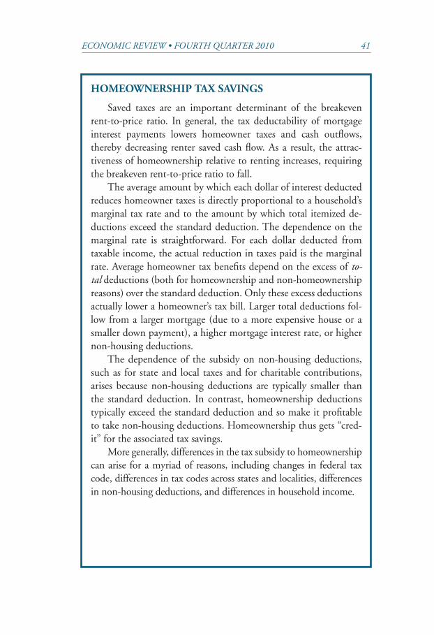
HOMEOWNERSHIP TAX SAVINGS

Saved taxes are an important determinant of the breakeven rent-to-price ratio. In general, the tax deductability of mortgage interest payments lowers homeowner taxes and cash outflows, thereby decreasing renter saved cash flow. As a result, the attrac-tiveness of homeownership relative to renting increases, requiring the breakeven rent-to-price ratio to fall.

The average amount by which each dollar of interest deducted reduces homeowner taxes is directly proportional to a household’s marginal tax rate and to the amount by which total itemized de-ductions exceed the standard deduction. The dependence on the marginal rate is straightforward. For each dollar deducted from taxable income, the actual reduction in taxes paid is the marginal rate. Average homeowner tax benefits depend on the excess of to-tal deductions (both for homeownership and non-homeownership reasons) over the standard deduction. Only these excess deductions actually lower a homeowner’s tax bill. Larger total deductions fol-low from a larger mortgage (due to a more expensive house or a smaller down payment), a higher mortgage interest rate, or higher non-housing deductions.

The dependence of the subsidy on non-housing deductions, such as for state and local taxes and for charitable contributions, arises because non-housing deductions are typically smaller than the standard deduction. In contrast, homeownership deductions typically exceed the standard deduction and so make it profitable to take non-housing deductions. Homeownership thus gets “cred-it” for the associated tax savings.

More generally, differences in the tax subsidy to homeownership can arise for a myriad of reasons, including changes in federal tax code, differences in tax codes across states and localities, differences in non-housing deductions, and differences in household income.


Lastly, the rate of house price appreciation is an obvious determi-nant of the breakeven rent-to-price ratio. Faster appreciation increases homeowner final wealth. To match it, renter new investments in stocks and bonds must increase. Doing so requires larger saved cash flow and thus a lower breakeven rent-to-price ratio. Conversely, slower house price appreciation requires lower renter saved cash flow to equalize final wealth and hence a higher rent-to-price ratio.

Market rent-to-price ratio

To determine whether ownership or renting builds more wealth, the breakeven rent-to-price ratio can be compared to a market rent-to-price ratio. This market ratio measures the rent relative to the pur-chase price of identical houses. When the market ratio falls below the breakeven ratio, rents are inexpensive relative to purchase prices, which allows renting to build more wealth. Conversely, when the market ratio rises above the breakeven ratio, rents are expensive relative to purchase prices, and so homeownership builds more wealth.

However, the comparison of breakeven and market ratios is com-plicated by some measurement limitations. Accurately estimating the market rent-to-price ratio is extremely difficult (see Appendix 2). The challenge is that no two houses are identical. In practice, it is necessary to use statistical estimates of rent values for owner-occupied houses and of purchase prices for renter-occupied houses. Unfortunately, such es-timates are typically biased by failing to account for numerous house attributes for which information is not readily available.

Because of these measurement challenges, the present analysis relies on ranges of plausible values for the market rent-to-price ratio, rather than on specific estimates. Many potential market ratios are simply too low or too high to be plausible. For example, a potential market rent that far exceeds homeownership cash outflows would cause all house-holds to purchase a house. Of course, this would be counterfactual, making such a high market ratio implausible.

The breakeven rent-to-price ratio is compared to two ranges, which can reasonably be expected to include all plausible market rent-to-price ratios. The first, broader range runs from 500 to 1,000 (all market and breakeven rent-to-price ratios will be expressed as monthly rent per $100,000 purchase price).8 The lower bound of 500, assumed to be


fixed from 1970 to 1999, is the approximate average ratio of median rent to median owner-estimated purchase price as reported in various Census Bureau surveys from 1970 through 2008.9 As described in Ap-pendix 2, unobserved house characteristics and upward-biased valua-tions by owners suggest that the true market rent-to-price ratio will be higher than 500. The upper bound of 1,000 is also assumed to be fixed from 1970 to 1999. One thousand is consistent with the highest average rent-to-price ratio found in a 20-year study that asked renters and homeowners to estimate the dollar amounts at which the house they lived in could be rented out and the price at which it could be sold (Garner and Verbrugge).10

Estimates of the growth rate of the market rent-to-price ratio sug-gest a narrower range of plausible market ratios. The growth rate of the market ratio, unlike its level, can be estimated with some accuracy. It simply equals the growth of rents minus the growth of house prices, and reasonable estimates exist for both.11 The upper and lower bounds on plausibility should grow at the same rate at which the actual market ratio grows.12 A time-varying upper bound on plausible market ratios can therefore be constructed as the highest time path that grows at the market ratio rate without exceeding 1,000 (Chart 1). Similarly, a time-varying lower bound on plausible market ratios can be constructed as the lowest time path that grows at the market ratio rate without falling below 500.

II. HISTORICAL EVIDENCE

Based on the analytical framework just described and historical data, this section compares the wealth built by homeownership and renting for ten-year occupancies beginning in 1970 through 1999. Spe-cifically, it constructs breakeven rent-to-price ratios for each of these initial years and then compares them to the fixed and time-varying, market-based ranges described in the previous section. Last, the section calculates the differences in final wealth between renting and owning when the market and breakeven ratios differed.

Historical breakeven ratios

The initial-period rent-to-price ratio that equated the final wealth of renters and homeowners has varied considerably over time. Based on


Chart 2BREAKEVEN RENT-TO-PRICE RATIO

0

200

400

600

800

1,000

0

200

400

600

800

1,000

1970 1975 1980 1985 1990 1995 2000

Initial Year of 10-Year House Occupancy

Initial monthly rent per $100,000 purchase price that equates wealth built over 10 years

Investing in Bonds

Investing in Stocks

Sources: See technical appendix

Chart 1RANGES OF PLAUSIBLE MARKET RENT-TO-PRICE RATIOS


0

200

400

600

800

1,000

0

200

400

600

800

1,000

1970 1975 1980 1985 1990 1995 2000 Initial Year of 10-Year Occupancy

monthly rent per $100,000 price

Fixed Upper Bound

Time-varying Upper Bound

Time-varying Lower Bound

Fixed Lower Bound


THE RISKS OF HOMEOWNERSHIP

For tractability, the article’s analysis makes a number of sim-plifying assumptions. These include: all house prices grew at the ex-post, nationally representative rate; all households stayed in their houses for exactly ten years; and all households and houses experienced no idiosyncratic events. Each of these assumptions ob-scures some significant risks. In particular, homeowners are subject to at least three overlapping types of risk: price risk, house risk, and household risk. Together such risks are substantial, which im-plies that the estimated breakeven rent-to-price ratios may be too low. More specifically, negative events falling into one or more of these risk categories may increase homeowner cash outflows and decrease homeowner final wealth. Taking account of this possibil-ity, a household would favor renting over owning at the breakeven rent-to-price ratio calculated in the main text. To restore indiffer-ence requires the breakeven rent-to-price ratio to rise.

The price risk associated with homeownership has several components. The first is the large variation over time and across locations in average home price appreciation. Price appreciation can even differ substantially across neighboring houses. The final wealth impact of the underlying house price swings are magnified by leverage. For example, a moderate price decline on a house can wipe out a homeowner’s equity. Lack of diversification further com-pounds price risk. For more than half of all homeowners, home equity accounts for at least two-thirds of household wealth (Sinai and Souleles 2009). A final component of homeownership’s price risk is illiquidity. Selling a house takes time. To quickly access ac-cumulated equity, a homeowner may be forced to accept a steep price discount.

The second category of homeownership risk concerns the spe-cific house itself. Numerous events can affect the consumption value that flows from a house. While such events typically cause price changes and so also fall into the price risk category, they separately affect a homeowner’s welfare as well. For example, serious damage to a house will likely require significant homeowner time and en-


ergy, regardless of any monetary costs the homeowner must bear. As another example, changes in the character of a neighborhood or metro area—such as to public school quality or crime—will affect homeowners’ welfare directly, in addition to affecting house values.

The third category of homeownership risk concerns house-holds themselves. It is common for a household to need to move unexpectedly. Shorter stays imply fewer years over which to amor-tize buying, selling, and any refinancing costs.

Of course, renting also poses significant risks. Renters face unknown future rents. Rents that increase rapidly will decrease renter wealth and so make homeownership relatively more attrac-tive (Sinai and Souleles 2005). Real returns on stocks and bonds, the primary savings alternatives to homeownership, are uncertain. In addition, some of the risks to homeownership just described also apply to renters. A decline in neighborhood quality affects the welfare of all local residents. But an important difference between owners and renters is that it is typically far less costly for a renter to move in response to a change in neighborhood quality.

A final point is that the identified risks also can yield posi-tive surprises. For example, crime may go down or public school quality may improve. But substantial economic research finds that people are “risk averse”: they prefer no surprises to the possibility of either a negative or a positive surprise. The more risk averse a household is, the higher the rent-to-price ratio must be to make it indifferent between renting and buying.


renters investing saved cash flow in bonds, rising mortgage interest rates pushed up the breakeven rent-to-price ratio from just 100 (monthly rent per $100,000 purchase price) in 1970 to above 600 for most of the 1980s (Chart 2).13 This increase in the bond-based breakeven ratio suggests that homeownership went from being a very effective way to build wealth during the early 1970s to a considerably less effective way during the 1980s. Falling mortgage interest rates and accelerating house appreciation pushed the bond-based breakeven ratio back below 200 by the mid-1990s, after which it began rising again.

Based on renters investing saved cash flow in stocks, the break-even ratio varied even more widely.14 Rising mortgage interest rates and returns from investing in stocks pushed the breakeven ratio up from about 200 in the early 1970s to above 800 for the entire 1980s (Chart 2, black line). Falling mortgage interest rates and stock returns, along with accelerating house appreciation, pushed the stock-based breakev-en ratio down sharply during the early and mid-1990s.15

The rise in breakeven rent-to-price ratios that began in the late 1990s was driven primarily by the large contraction of house prices from 2007 to 2009.16 The ten-year occupancy that began in 1996 was the last to end prior to the price contraction. During this occupancy, prices appreciated every year. Consequently, houses purchased in 1996 had cumulative real price increases of almost 60 percent. In contrast, houses purchased three years later, in 1999, experienced just seven years of strong price appreciation, followed by three years of contraction. The corresponding cumulative real price increase was under 20 percent.17

Breakeven rent-to-price ratios are likely to continue to rise through occupancies beginning in 2006. Hence, homeownership will continue losing its effectiveness as a way to build wealth. This expectation is pre-mised on house prices continuing to contract in 2010 and then stabiliz-ing at their late 2010 level.18 If this assumption proves correct, ten-year rates of price appreciation on houses purchased in 2000 through 2006 will continue to fall. Regardless of purchase year, these houses will have experienced four years of falling prices. But as the year of purchase ad-vances, they will have experienced fewer of the preceding boom years. Lower house price appreciation, in turn, allows renter households to afford higher rents while matching dampened homeowner final wealth. Equivalently, lower house price appreciation implies an increase in the


breakeven rent-to-price ratio, reflecting that homeownership has be-come a relatively less effective way to build wealth.19

Breakeven rent-to-price ratios for occupancies beginning in 2006 through 2010 will also be driven by the recent price contraction, only in the opposite direction. Advancing through these five purchase years, the number of years of price decline that will have been experienced will fall from four to zero assuming that prices indeed fall in 2010 and stabilize thereafter. The decrease in the number of years of price con-traction will put downward pressure on the breakeven ratio. In other words, during these purchase years homeownership may become a more effective way to build household wealth (although not necessarily more effective than renting).

Of course, at some point house prices will start appreciating again. This appreciation will put downward pressure on the breakeven ratio for occupancies that began as many as ten years earlier. For example, house prices that begin appreciating again in 2011 would put down-ward pressure on the breakeven ratio for years 2001 through 2010.20

Complementing a possible fall in the breakeven ratio is that the market ratio rose sharply from 2006 to 2010. This simply reflects the fall in house prices over the years.

Hence the breakeven ratio need not be as low as in the past for homeownership to be the more effective way to build household wealth.

Comparing breakeven and market rent-to-price ratios

To determine whether renting or purchasing a house built more wealth over a given ten-year occupancy, the historical breakeven rent-to-price ratios just described can be compared to the two plausible ranges of the market rent-to-price ratio introduced in the previous sec-tion. As a first pass, the historical breakeven ratios will be compared to the broader plausible range, characterized by a fixed lower bound of 500 and a fixed upper bound of 1,000. The ratios will then be com-pared to a plausible range based on time-varying bounds.

For initial years of occupancy in which the breakeven ratio fell below the lower bound of the plausible market range, owning unam-biguously built more wealth than renting. In this case, the rent (for a given house price) a renter could afford while still matching a home-owner’s final wealth was simply too low to be plausibly available. When


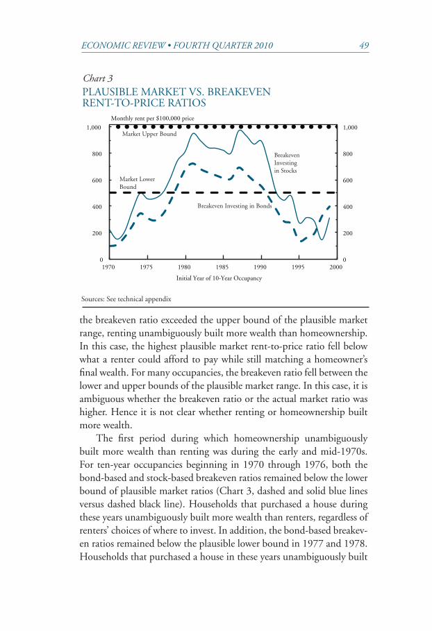
the breakeven ratio exceeded the upper bound of the plausible market range, renting unambiguously built more wealth than homeownership. In this case, the highest plausible market rent-to-price ratio fell below what a renter could afford to pay while still matching a homeowner’s final wealth. For many occupancies, the breakeven ratio fell between the lower and upper bounds of the plausible market range. In this case, it is ambiguous whether the breakeven ratio or the actual market ratio was higher. Hence it is not clear whether renting or homeownership built more wealth.

The first period during which homeownership unambiguously built more wealth than renting was during the early and mid-1970s. For ten-year occupancies beginning in 1970 through 1976, both the bond-based and stock-based breakeven ratios remained below the lower bound of plausible market ratios (Chart 3, dashed and solid blue lines versus dashed black line). Households that purchased a house during these years unambiguously built more wealth than renters, regardless of renters’ choices of where to invest. In addition, the bond-based breakev-en ratios remained below the plausible lower bound in 1977 and 1978. Households that purchased a house in these years unambiguously built

Chart 3PLAUSIBLE MARKET VS. BREAKEVEN RENT-TO-PRICE RATIOS

0

200

400

600

800

1,000

0

200

400

600

800

1,000

1970 1975 1980 1985 1990 1995 2000

Initial Year of 10-Year Occupancy

Monthly rent per $100,000 price

Breakeven Investing in Bonds

BreakevenInvestingin Stocks

Market LowerBound

Market Upper Bound



more wealth than a household that rented an identical house and in-vested the saved cash flow in bonds. However, the stock-based break-even ratio in these two years was above the lower bound of the plausible range of market ratios. Hence it is possible that either purchasing a home in 1977-78 or renting one and investing the saved cash flow in stocks would have built more wealth.21

For ten-year occupancies beginning in the late 1970s through the early 1990s, both the bond-based and stock-based breakeven ratios re-mained within the broad range of plausible market ratios defined by the fixed 500 and 1,000 bounds. Hence, using this broad range of plausi-bility, it is not possible to say with certainty whether renting or home-ownership built more wealth. For several of years during the 1980s, however, the breakeven ratio rose very close to the upper bound on plausibility. For occupancies beginning in such years, it is likely that the actual market rent-to-price ratio, as opposed to the plausible range, was below the breakeven ratio, implying that renting built more wealth than homeownership.

Homeownership again unambiguously built more wealth than did renting for ten-year occupancies beginning during most of the 1990s. The bond-based breakeven rent-to-price ratio fell below the 500 lower bound for occupancies beginning in 1991; the stock-based breakeven ratio fell below it for occupancies beginning in 1993. Both breakevens remained below the 500 lower bound through at least 1999. Of course, it is not surprising that homeownership built more wealth than renting for occupancies that coincided with a period of very fast house price appreciation.22

In contrast, homeowners who began their ten-year occupancies from 2000 through 2006 will experience at least four years of falling prices. If, as assumed above, prices stabilize at their 2010 level, the number of positive appreciation years experienced during these occu-pancies will fall from five to zero. As a result, the breakeven ratio for at least the more recent of these years is likely to be sufficiently high to make renting the more effective way to build household wealth. On the other hand, if significant house price appreciation resumes in 2011 or shortly thereafter, the rise in the breakeven ratio will be at least partly tempered.


Chart 4TIME-VARYING PLAUSIBLE MARKETVS BREAKEVEN RENT-TO-PRICE RATIOS


Comparing breakeven ratios with the time-varying range of market ratios

As described in the first section, reasonably estimated changes in rents and house prices imply changes over time in the market rent-to-price ratio, whatever its initial level.23 Taking account of these changes yields narrower, time-varying bounds on the market rent-to-price ratio.

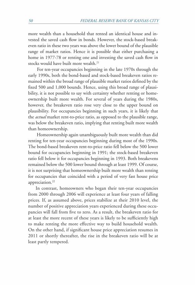
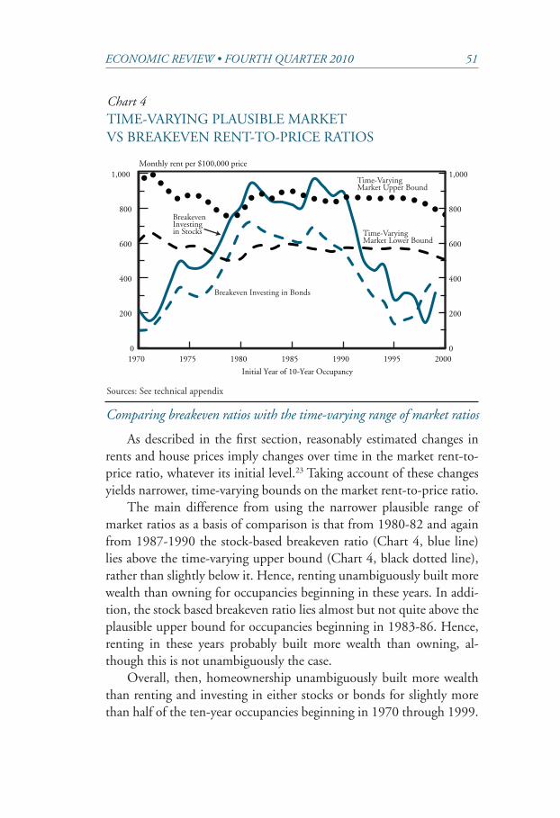
The main difference from using the narrower plausible range of market ratios as a basis of comparison is that from 1980-82 and again from 1987-1990 the stock-based breakeven ratio (Chart 4, blue line) lies above the time-varying upper bound (Chart 4, black dotted line), rather than slightly below it. Hence, renting unambiguously built more wealth than owning for occupancies beginning in these years. In addi-tion, the stock based breakeven ratio lies almost but not quite above the plausible upper bound for occupancies beginning in 1983-86. Hence, renting in these years probably built more wealth than owning, al-though this is not unambiguously the case.

Overall, then, homeownership unambiguously built more wealth than renting and investing in either stocks or bonds for slightly more than half of the ten-year occupancies beginning in 1970 through 1999.

0

200

400

600

800

1,000

0

200

400

600

800

1,000

1970 1975 1980 1985 1990 1995 2000


Monthly rent per $100,000 price

Time-VaryingMarket Upper Bound

Time-VaryingMarket Lower Bound

Breakeven Investingin Stocks

Breakeven Investing in Bonds


These were primarily during the early and mid-1970s and most of the 1990s. Renting and investing in stocks unambiguously built more wealth than owning for one quarter of these ten-year occupancies, all during the 1980s. For the remaining quarter of the occupancies, either homeownership or renting and investing may have built more wealth, although for several of these years during the 1980s, renting was con-siderably more likely to have done so.

For many of the ten-year occupancies currently underway, it is likely that renting will prove to have unambiguously built more wealth than owning. The breakeven ratio is likely to rise sharply through occupan-cies beginning in 2006. Complementing this rise in the breakeven ratio is that the run-up of house prices relative to rents through 2006 pushed the time-varying upper bound on plausibility downward, from just un-der 800 in 1999 to approximately 600 in 2005-07. An upper bound on the plausible market rent-to-price ratio of 600 would have doubled the number of occupancies beginning in 1970-1999 for which renting and investing saved cash flow built more wealth than homeownership.

The payoff from choosing between renting and owning

To this point, the analysis has focused on determining whether renting or owning a house built more wealth over a succession of ten-year occupancies. But how large was the wealth gain or loss from choos-ing one tenure type rather than the other? Did choosing “correctly” yield a sizable difference in wealth?

The answer is clearly “yes” for most years. When the rent-to-price ratio differed from the breakeven ratio, the difference in final wealth between renting and purchasing was typically quite large. For example, when the market ratio was 10 percent above the bond-based breakeven ratio, rent-ing and investing in bonds would have resulted on average across ten-year occupancies in final wealth that was 12 percent lower than a homeowner’s final wealth. When the market ratio was 10 percent lower than the bond-based breakeven ratio, renting and investing in bonds resulted, on aver-age, in final wealth 12 percent higher than a homeowner’s final wealth. Across ten-year occupancies, the corresponding differences in final wealth ranged from 2 to 26 percent.

For stock-based breakeven ratios, a 10 percent difference with the market ratio would have caused an average final wealth difference of 24


percent. The corresponding range across ten-year occupancies was 2 to 62 percent.24 These wealth differences scale proportionally to alternative percent differences between the breakeven and market rent-to-price ratios.

Of course, this large payoff is based on hindsight. While a cur-rent year’s market rent-to-price ratio is based on current information, a current year’s breakeven rent-to-price ratio is based on numerous un-knowns, including house prices, stock prices, bond prices, mortgage interest rates, and the tax code over the subsequent ten years.

III. SUMMARY AND CONCLUSIONS

Conventional wisdom has long suggested that homeownership is an effective way to build household wealth. Consistent with this belief, homeownership is often considered to be a key part of the American Dream. Yet, the loss of a house to foreclosure recently experienced by millions of U.S. households, along with the sharp declines in wealth experienced by virtually all U.S. homeowners, would seem to make a reconsideration of homeownership inevitable.

The analysis in this article shows that while homeownership often builds more household wealth than renting and investing the saved cash flow, it also often does not. More specifically, for most ten-year occupan-cies beginning during the 1970s and 1990s, homeownership unambigu-ously built more wealth. In contrast, for most occupancies beginning dur-ing the 1980s, renting and investing unambiguously built more wealth. Renting and investing is also likely to build more wealth than homeown-ership for many of the occupancies that started in 2000 through 2009.

These results suggest that either homeownership or renting and investing can be reasonable strategies for building household wealth. In other words, the conventional wisdom that homeownership is usu-ally the better strategy is probably too strong. For many households in many years, renting and investing the saved cash flow has built more wealth than homeownership. On the other hand, about half of the time, homeownership has built more wealth than renting. Moreover, it may be easier to purchase than to rent a house that closely matches a house-hold’s unique tastes. Put differently, identical houses are typically not available both to rent and to purchase.

A more balanced view of the relative advantages and disadvantages of homeownership could have important macroeconomic implica-


tions. On the one hand, demand may shift away from single-family houses and delay the recovery of single-family construction. On the other hand, a demand shift away from homeownership might increase household savings invested in stocks, bonds, and other financial securi-ties. This, in turn, would likely contribute to lower intermediate- and long-term interest rates, stimulating business investment and increas-ing the economy’s nonresidential productive capacity. Finally, while a more balanced view of homeownership would likely increase the share of households living in multifamily homes, it would also increase the affordability of many other things that households consume.


APPENDIX 1

THE CONSUMPTION VALUE OF HOMEOWNERSHIP

The analysis in the text of whether renting or homeownership built more wealth implicitly focused on homeownership’s investment benefit. Homeownership’s other main benefit, having a place to live in and enjoy, was removed from the analysis by assuming that owners and renters lived in identical houses and so received the same consumption benefit.

This appendix compares the relative size of homeownership’s con-sumption and investment benefits. Specifically, it compares the con-sumption value of living in a house for a ten-year occupancy against the net proceeds from selling the house at the end of that occupancy. Homeownership’s cash outflows, which are used to “purchase” the con-sumption and investment benefits, do not enter into the calculations of the benefits in this appendix. Hence these benefits can be consid-ered gross of costs. The estimates indicate that, for ten-year occupan-cies beginning in 1970 through 1999, homeownership’s consumption benefit typically far exceeded homeownership’s investment benefit. In other words, homeownership’s large cash outflows primarily purchased consumption rather than investment.

Investment benefit

As just described, the investment benefit to homeownership is the net proceeds from selling the house. These proceeds are discounted back to the time of the house purchase using the after-tax, one-year Treasury bill rates that applied over the ten-year occupancy. The result equals the investment in one-year Treasury bills at the time of purchase that over ten years would grow, if continually reinvested after paying taxes on interest, to the net proceeds from the sale of the house.

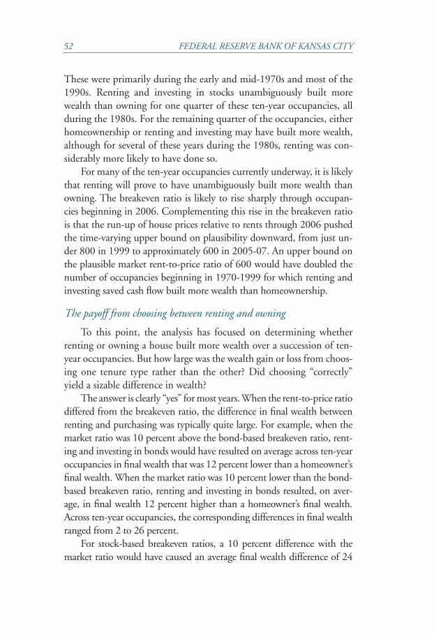
Homeownership’s investment benefit has varied widely over time. The most important underlying determinant is the rate of house price appreciation. Correspondingly, the investment benefit—measured relative to a house’s purchase price—was highest for occupancies be-ginning in the early 1970s and mid 1990s (Chart 5, solid blue line). During both periods, the investment benefit rose above $70,000 (per $100,000 purchase price). Conversely, the investment benefit was espe-cially low for occupancies beginning during the 1980s, remaining close


to $30,000 for the entire decade. Averaged across all 29 years of initial purchase, the investment benefit was $46,500.

Consumption benefit

The consumption benefit depends on the market rent-to-price ra-tio and so cannot be estimated precisely. Like the market ratio, it is instead best described by a range of plausible values. In addition, the consumption benefit “flows” continuously over a ten-year occupancy. In practice, this consumption flow is assumed to take place at a limited number of points in time and then discounted from each of these back to the time of purchase.

The flow of homeownership’s consumption benefit—that is, hav-ing a place to live in and enjoy—is naturally valued by the market rent that would have to be paid to live in an identical house. Such a rent relative to the identical house’s purchase price is exactly the market rent-to-price ratio discussed in the main text. Because the market ratio is known only up to a plausible range, homeownership’s consumption benefit valuation can only be calculated to a plausible range as well.

The consumption benefit flows that correspond to purchasing a house at the lower-and upper-bound plausable market ratios can be dis-counted to the time of purchase using after-tax, one-year Treasury bill

Chart 5VALUING OWNERSHIP BENEFITS

0

20,000

40,000

60,000

80,000

100,000

120,000

0

20,000

40,000

60,000

80,000

100,000

120,000

1970 1975 1980 1985 1990 1995 2000


Upper Bound Consumption Benefit

Lower Bound Consumption Benefit

Investment Benefit

Valuation in year of purchase per $100,000 purchase price



rates. The results equal the lower-bound and upper-bound investments in one-year Treasury bills at the time of purchase that, if continually reinvested, would pay, year by year, the lowest and highest plausible market rent for the owned house.

The range of plausible consumption benefit valuations turns out to be relatively wide. Comparing the dotted and dashed black lines in Chart 5 shows that the upper-bound valuation exceeded the lower bound by an average of $32,000 (per $100,000 purchase price). Even so, the lower-bound consumption benefit typically exceeded the invest-ment benefit by a wide margin (Chart 5, dashed black line versus solid blue line). On average across years, the margin was almost 50 percent.

The upper-bound consumption benefit valuation always far ex-ceeded the investment benefit (Chart 5, dotted black line versus solid blue line). Even for the occupancies in which investment benefits were highest, the upper-bound consumption benefit was at least 25 percent higher. For occupancies with a below-average investment benefit, the upper-bound consumption benefit was as much as three times higher.

Homeownership, at least until recently, was often described as a great investment that also includes a place to live. More accurately, homeownership should have been described as a place to live that also includes an expected investment benefit. This shift in emphasis applies not only to homeownership occupancies that coincided with the recent sharp price contraction. Even for ten-year occupancies that ended prior to the contraction, homeownership’s principle benefit has almost al-ways been having a place to live in and enjoy. For ten-year occupancies currently underway, this is likely to be even more the case.


APPENDIX 2

ESTIMATING THE MARKET RENT-TO-PRICE RATIO

Estimates of market rent-to-price ratios are typically based on sta-tistical estimates of rent values for owner-occupied houses and of pur-chase prices for renter-occupied houses. Such estimates are based on shared attributes between very large samples of both types of houses.

The measured attributes available to make statistical estimates, however, typically miss many important determinants of rents and pur-chase prices. Examples of such “unobserved” attributes include numer-ous characteristics of a house itself, such as square footage, state of re-pair, and aesthetic appeal; the location characteristics of a house’s plot, such as adjacent traffic, noise, and scenic views; and the characteristics of a house’s neighborhood, such as property taxes, public school qual-ity, and crime. These unobserved attributes tend to be more desirable for owner-occupied houses and so cause estimates of the market rent-to-price ratio to be understated. In other words, a rented house that appears statistically identical to an owner-occupied house is often less desirable. Reasons why unobserved attributes may be more desirable include the typically higher income of owners and the fact that they have more incentive to keep their house in good repair.

Understated estimates of the market rent-to-price ratio, in turn, exaggerate the saved cash flows that renters can invest in stocks and bonds, thus overstating a renters’ final wealth. Correcting for this bias would increase the chances that the market rent-to-price ratio is above the breakeven ratio, in which case owning would build more wealth than renting.

The difficulty in estimating market rents on owner-occupied houses and market purchase prices on rented houses is approximate-ly matched by the difficulty in estimating market purchase prices of owner-occupied houses. Estimated owner-occupied market prices are often based on homeowners’ self-assessments. Research suggests that owners tend to overestimate their house’s market price, thereby bias-ing downward estimates of the market rent-to-price ratio (Ihlanfeldt and Martinez-Vazquez ; Goodman and Ittner). Similar to the case of underestimated rents, correcting for overestimated market house prices would increase the chances that the correctly measured market rent-to-


price ratio is above the breakeven ratio, in which case owning would build more wealth than renting. Equivalently, purchasing a house may be less expensive than estimated and so, more attractive.


ENDNOTES

1In theory, a net present value comparison could be applied to the same cash flows tracked in the analysis. The considerable challenge would be to choose an appropriate discount rate. As the opportunity cost of funds varies over the years, the discount rate would have to vary as well. It would also have to account for taxes, which affect the opportunity cost of funds. An additional complication is that taxes depend on household characteristics, in particular on a household’s tax bracket, which in turn depends on investment income. The main benefit of comparing the final wealth between owners and renters, which is the basis for the analysis, is that discounting is not required. Instead, after-tax rates of return implicitly discount flows to the end of each ten-year occupancy.

2The requirement that the houses are identical is meant to imply that the two households’ “consumption” of housing is equal. Appendix 1 compares the consumption benefits of homeownership to its pure investment benefits. How-ever, the consumption value of living in a house may also depend on whether a household rents or owns it. For example, homeowners may enjoy homeownership tasks such as home maintenance and gardening, or homeowners may take pride in owning their home. Alternatively, the considerable time requirements associated with homeownership can be interpreted as lowering housing consumption.

3Ten years is a rough estimate of the average time that a household lives in a house after purchasing it. Generally accepted estimates on the expected stay of new home buyers do not exist. The average stay among home sellers is seven years (Na-tional Association of Realtors). But sellers are a self-selected group with a shorter-than-average expected duration of occupancy. Hence, the expected stay across all new buyers will be somewhat longer than seven years. A ten-year horizon represents a rounding up from the seller average stay to an easily recognized time horizon.

4This equality of rent plus new investment with the sum of homeownership payments requires that the renter reinvest all dividends and interest payments net of taxes.

5Figure 1 and the associated description of owner and renter wealth building by necessity leave out many important details. A more comprehensive description is included in the technical appendix, which is available online.

6An important exception is that tax considerations can make the breakeven rent-to-price ratio depend on the purchase price level. As explained in the accompa-nying box, homeowners’ tax savings are proportional to the excess of total itemized deductions above the standard deduction. The higher an initial mortgage, the higher is the share of homeowner deductions that are above the standard deduction.

7Homeowner payments, including for principal, can be thought of as the “cost” of achieving homeowner final wealth. In other words, final wealth is a gross rather than a net benefit.


8Like the breakeven ratio, the market rent-to-price ratio for any year does not depend on the broad price level. Hence the market ratio is comparable across years.

9All prices are for single-family, detached houses with three bedrooms, as reported in the 1970 through 2000 decennial censuses and the 2008 American Community Survey. Three is the median number of bedrooms among owner-occupied, single-family detached houses on no more than ten acres of land. The ratio of median monthly contract rent—which includes utility expenses for some units but not all—to median owner-estimated purchase price (adjusted to be measured in terms of monthly rent per $100,000 purchase price) ranged from 444 to 532 across the various decennial censuses and the 2008 American Com-munity Survey. The likelihood that the houses on which rent were paid had, on average, less desirable unobserved attributes than owner-occupied houses implies that the rent-to-price ratio on an identical unit would be above this. At least partly offsetting this is that a complete exclusion of utility expenses from contract rent would push the market rent to price ratio lower. Consistent with a lower bound of 500, a recent study that used statistical techniques to control for variations in observed attributes estimated a rent-to-price ratio between 375 and 500 (Davis, Lehnert, and Martin). The study did not control for unobserved attributes and so

the actual rent-to-price ratio is likely to be higher. 10Such price and rent valuations were on the same house and thus unob-

served attributes were held constant. The study, jointly conducted by the Census Bureau and the Bureau of Labor Statistics, ran from 1982 to 2002 in five large metro areas: New York, Los Angeles, Chicago, Houston, and Philadelphia. Hous-ton’s estimated price-to-rent ratio, which was consistently the highest among the five metro ratios, usually remained above 850. During the early 1990s, it rose to approximately 1,000. A different study, consistent with an upper bound of 1,000, was conducted in 1974 by the American Council of Life Insurance. Based on estimated prices and rents of 43,000 properties, it found an average rent-to-price ratio of 987 (Peiser and Smith).

11Specifically, the growth of rent for houses similar in characteristics to own-er-occupied houses is measured the owner equivalent rent (OER) component of the consumer price index. Growth of house prices is measured by several re-spected “repeat sales” house price indexes. These estimated rent and price changes are “constant quality” in the sense that they are based on changes over time of the rent or sales price of the same house.

12Suppose the highest plausible rent-to-price ratio for a year is 1,000 and that the actual market ratio subsequently grows. The upper-bound plausible ratio must increase as well. Otherwise, if the actual market ratio were indeed at its upper bound prior to the growth, the actual rent-to-price market ratio would become implausible, which is a contradiction.

13The bond-based breakeven rent-to-price ratios are based on investments in one-year Treasury bills that are continually rolled over after paying taxes on interest.


14Stock capital appreciation and dividends are assumed to be the same as for the Standard and Poor’s 500 index. Capital gains taxes are assumed to be paid annually. This biases downward the stock-based breakeven rent-to-price ra-tio relative to paying capital gains taxes only at the end of a ten-year occupancy. Offsetting this bias is the exclusion of state and local income taxes in the current calculation. In many states, mortgage interest can be deducted from taxable in-come. In addition, a renter’s interest, dividend, and capital gains are often subject to state and local income taxes. In both cases, state and local taxes increase the relative attractiveness of homeownership.

15For better intuition on magnitudes, the breakeven rent-to-price ratio can be converted to the threshold rent on a baseline quality house (rather than the breakeven rent on a $100,000 house). For example, the baseline quality might be assumed to be that of a representative house with median price in 2000. This median price can be deflated, using the total and owner equivalent rent CPI indexes, to give the real price of a similar house in other years. Adjusting the breakeven rent-to-price ratios discussed in the main text to correspond to this real baseline-quality purchase price gives the threshold rent that equates final wealth between purchasing and renting a baseline-quality house. During the early 1970s, real threshold rents on such a baseline house ranged from $125 (bond-based) to $275 (stock-based, 2009 dollars). As is intuitive, these threshold rents are quite low. During the 1980s, in contrast, the stock-based threshold rent stayed above $1,000, which is quite high. During most of the 1990s, threshold rents remained below $600 and in some years dropped as low as $200.

16Separately, the decrease in the stock-based breakeven ratio below the bond-based one in the late 1990s stems in part from financial swings associated with the 2001 and 2007-09 recessions. In particular, the S&P 500 contracted by just over a third from 2000 to 2002, following a strong run-up the previous five years. It then contracted by 40 percent in 2008, a third of which was recovered the subsequent year. As discussed in the text, weak returns on investments cause the breakeven ratio to rise.

17The S&P/Case-Shiller National Home Price Index estimates that house price swings were somewhat wider than the house price swings estimated by the Freddie Mac Repeat Sales House Price Index used in the analysis. For example, Case-Shiller estimates cumulative real house price appreciation for the ten-year occupancy that began in 1996 to be 80 percent rather than 57 percent. It esti-mates cumulative real appreciation for the ten-year occupancy starting in 1999 to be 7 percent rather than 18 percent. Hence the 1996-99 rise in the breakeven ratio calculated using the Case-Shiller index would be considerably larger and steeper than the rise shown in Chart 2. Correspondingly, the increase in the rela-tive attractiveness of renting compared to homeownership over these purchase years would be considerably larger. On the other hand, the breakeven ratio during


the 1990s would likely be considerably lower if calculated using the Case-Shiller index, implying that homeownership was an even more attractive way to build household wealth than is implied in the analysis.

18The expectation of falling prices in 2010 reflects that through the third quarter of 2010, repeat-sales house price indexes are down by as much as 2.3 percent from their level in late 2009.

19Partly dampening the upward movement of the stock-based breakeven ra-tio is the crash in stock prices during 2008. As of late 2010, the S&P index value remains more than 20 percent below its December 2007 average. The relatively smaller decline in housing prices, as measured by the Freddie Mac index, may nevertheless outweigh the stock price decline because of the leverage associated with homeownership.

20Complementing a possible fall in the breakeven ratio is that the market rent-to-price ratio rose sharply from 2006 to 2010. This simply reflects the fall in house prices over these years. Further contributing to the possibility that the breakeven ratio will fall below the range of plausible market ratios is that the upper and lower bounds on plausibility have risen sharply since 2006, reflecting the contraction in house prices. Hence the breakeven ratio need not be as low as in the past for home-ownership to be the more effective way to build household wealth.

21This ambiguity does not imply that the comparison of the breakeven and range of plausible market ratios is uninformative. The stock-based breakeven ra-tio in 1977 was 503, only slightly above the lower bound on plausibility. The lower a value within the plausible range, the more likely it is that the actual mar-ket ratio will be above it. While it cannot be ruled out that the 1977 market ratio was less than 503, almost certainly it was higher.

22The period of rapid real house price growth, as measured by several repeat sales house price indexes, lasted from 1997 to 2006, with the fastest growth oc-curring from 2001-05.

23For the present analysis, the growth of house prices is based on the Freddie Mac repeat sales house price index. The growth of rents is based on the owner equivalent rent (OER) component of the consumer price index. Both of these are “constant quality” in the sense that they are based on changes over time of the rent of the same house and the sales price of the same house. Additionally, the OER growth rate is based on changes in rents on renter-occupied houses that are averaged together using weights to match the average observed characteristics of owner-occupied houses.

24Correspondingly, a nominal $10 monthly difference between the market rent and the bond-based threshold rent on a median-priced house would have implied an average final wealth difference of $1,900 (nominal), with a range across occupancies of $1,500 to $2,400 (in absolute value). A nominal $10 monthly difference between the market rent and the stock-based threshold rent


on a median-priced house would have implied an average final wealth difference of $2,400, with a range across occupancies of $1,200 to $3,200.


REFERENCES

Davidoff, Thomas. 2006. “Labor Income, Housing Prices, and Homeownership,” Journal of Urban Economics, vol. 59, pp. 209-35.

Davis, Morris, and François Ortalo-Magné. 2010. “Household Expenditures, Wages, Rents,” Review of Economic Dynamics, forthcoming.

Freddie Mac. 2008. “Weekly Primary Mortgage Market Survey,” at www.freddi-emac.com/news/finance/docs/monthly_refi.xls, downloaded November 14.

Garner, Thesia I., and Randal Verbrugge. 2010. “The Puzzling Divergence of US Rents and User Costs, 1980-2004: Summary and Extensions,” in W. Erwin Diewert, Bert M. Balk, Dennis Fixler, Kevin J. Fox, and Alice O. Nakamu-ra, eds., Price and Productivity Measurement, vol. 1, Housing. Trafford Press: forthcoming.

Goodman, John L., and John B. Ittner. 1992. “The Accuracy of Home Owners’ Estimates of House Value,” Journal of Housing Economics, vol. 2, no. 4, De-cember, pp. 356-69.

Harding, John P., Stuart S. Rosenthal, and C.F. Sirmans. 2007. “Depreciation of Housing Capital, Maintenance, and House Price Inflation: Estimates from a Repeat Sales Model,” Journal of Urban Economics, vol. 61, pp. 193-217.

Himmelberg, Charles, Christopher Mayer, and Todd Sinai. 2005. “Assessing High House Prices: Bubbles, Fundamentals, and Misperceptions,” Journal of Eco-nomic Perspectives, vol. 19, no. 4, Fall, pp. 67-92.

Ihlanfeldt, Keith R., and Jorge Martinez-Vazquez. 1986. “Alternative Value Esti-mates of Owner-Occupied Housing: Evidence on Sample Selection Bias and Systematic Errors,” Journal of Urban Economics, vol. 20, no. 3, pp. 356-69.

Poterba, James, and Todd Sinai. 2008. “Tax Expenditures for Owner-Occupied Housing: Deductions for Property Taxes and Mortgage Interest and the Ex-clusion of Imputed Rental Income,” American Economic Review, vol. 98, no. 2, March, pp. 84-89.

Rappaport, Jordan. 2007. “A Guide to Aggregate House Prices,” Federal Reserve Bank of Kansas City, Economic Review, Second Quarter, pp. 41-72.

Sinai, Todd, and Nicholas S. Souleles. 2009. “Can Owning a Home Hedge the Risk of Moving?” NBER working paper 15462, October.

__________. 2005. “Owner-Occupied Housing as a Hedge Against Rent Risk,” Quarterly Journal of Economics, vol. 120, no. 2, May, pp. 763-89.

Shiller, Robert. 2010. Downloaded on March 10 at http://www.econ.yale.edu/~shiller/data/ie_data.xls.

Verbrugge, Randal. 2008. “The Puzzling Divergence of Rents and User Costs, 1980–2004,” The Review of Income and Wealth, vol. 54, no. 4, December, pp. 671-99.

Date post:	25-Mar-2022
Category:	Documents
Upload:	others
View:	2 times
Download:	0 times

The Effectiveness of Homeownership in Building Household ...

Documents