The Effectiveness of the Elliott Waves Theory to Forecast ... · theoretical elements of the wave...

International Business Research; Vol. 10, No. 6; 2017

ISSN 1913-9004 E-ISSN 1913-9012

Published by Canadian Center of Science and Education

1

The Effectiveness of the Elliott Waves Theory to Forecast Financial

Markets:

Evidence from the Currency Market

Eugenio D’Angelo1, Giulio Grimaldi

1

1Department of Economics and Legal Studies, Pegaso Telematic University, Naples, Italy

Correspondence: Eugenio D’Angelo, Department of Economics and Legal Studies, Pegaso Telematic University, Naples, Italy.

Received: March 31, 2017 Accepted: April 24, 2017 Online Published: May 4, 2017

doi:10.5539/ibr.v10n6p1 URL: https://doi.org/10.5539/ibr.v10n6p1

Abstract

The purpose of this paper is to investigate the capability of a technical analysis to be used as a valuable tool in

forecasting financial markets. After discussing the primary theoretical and methodological differences that

oppose the fundamental analysis and technical analysis and introducing the Elliott waves theory, the paper

focuses on the results obtained after applying this method to the currency market. The results show that during

the period from 2009-2015, the exchange rate between the U.S. dollar and euro could be forecasted with great

accuracy. A potential future pattern is also proposed for the exchange rate beginning in March 2017. The

research confirmed the usefulness of Elliott’s model for predicting currency markets, and the effectiveness of the fundamental analysis theories generally adopted for academic studies was evaluated.

Keywords: technical analysis; Elliott waves; currency market

1. Introduction

Financial market forecasting continues to be a core issue for academic scholars as well as professional investors.

In the financial field, predictions involve information analyses and influence the ways these analyses may drive decision-making processes when buying or selling financial assets.

Two types of approaches are usually adopted in the field of financial market prediction: fundamental analyses

and technical analyses. Professional investors and traders are typically more likely to support and use technical

analyses in predicting the market value of financial assets, while fundamental analyses are most commonly used

by academic researchers. The debate between these two approaches mainly focuses on the capabilities of their

various models to succeed in forecasting financial performance using different tools. Technical analysts use a

visual approach based on the application trend models on price charts, and fundamentalists use mathematical models to investigate and evaluate asset prices.

Fundamental analysts usually sustain the supremacy of their approach by arguing that their models are supported

by theory, which cannot be said for the technical approach to predicting asset prices. Moreover, theoretical and

empirical financial studies in the field of market efficiency assume a random walk model for asset pricing, which

excludes any possibility for technical analysts to forecast future prices (Fama, 1970). Thus, technical analyses

are also referred to as “voodoo finance,” and the difference between fundamental and technical analyses is argued to be similar to the difference between astronomy and astrology (Lo et al., 2000).

On the other hand, technical analysts argue that data previously collected contain important information that can

be used in predicting future prices and that their models are used by a multitude of traders and fund managers.

Moreover, some studies rejected the random walk theory and provided a large amount of evidence supporting

technical trading. Brock et al. (1992), Lo et al. (2000), LeBaron (1999), and Neely (2002), among others, argued that substantial gains exceeding the market gains could be made using a visual analysis (Zhu and Zhou, 2009).

The purpose of this exploratory study was to investigate the capability of one of the most commonly used

technical methods for financial market prediction: the Elliott waves theory. The method has been applied to the

currency market to verify whether the future exchange rates for the usd/euro could have been predicted using this

technical analysis. The forex market was chosen because there is evidence that a technical analysis could be a

http://ibr.ccsenet.org International Business Research Vol. 10, No. 6; 2017

2

useful tool for currency managers (Gehrig and Menkhoff, 2006).

The paper consists of three additional sections. In the second section, the primary traits of the Elliot waves

theory in predicting financial markets are presented. In the third section, the results obtained by the waves model in predicting the euro/usd exchange rate are provided. The final section discusses the conclusions.

2. Theoretical Background

The wave theory is the result of an analysis of the stock market carried out by Ralph Nelson Elliott in the 1930s,

but it is still relevant and used by many traders and institutional investors. To better understand the way the

waves theory was employed to assess financial assets in the empirical part of the paper, in this section, the main

theoretical elements of the wave theory according to the codification proposed by Prechter and Frost (1978) are described.

The Elliott waves theory, as all other technical analyses, mainly focuses on studying a time series in market prices and assumes that historic patterns are able to predict future patterns.

The Elliott model is composed of impulse waves (indicated by numbers) and corrective waves (indicated by

letters). There are several accepted annotations to label Elliott waves for the different degrees of tendency. For this work, the annotations listed in Table 1 were used.

Table 1. Elliott impulse waves and corrective wave labels in different degrees (source: adapted from Prechter and Frost, 1978)

Degree Labels for impulse waves Labels for corrective waves

Grand Supercycle [I] [II] [III] [IV] [V] [A] [B] [C]

Supercycle (I) (II) (III) (IV) (V) (A) (B) (C) Cycle I II III IV V A B C

Primary [1] [2] [3] [4] [5] [a] [b] [c]

Intermediate (1) (2) (3) (4) (5) (a) (b) (c)

Minor 1 2 3 4 5 a b c

Minute [i] [ii] [iii] [iv] [v] [a°] [b°] [c°]

Minuette (i)(ii)(iii)(iv)(v) (a°) (b°) (c°)

Subminuette i ii iii iv v a° b° c°

For each degree of a trend, an impulse wave is composed of five lower degree waves (sub-waves), and it moves

in the same direction of the higher-degree trend. On the other hand, corrective waves are composed of three lower degree waves, and they move against the higher degree trend.

When connected, impulse waves and corrective waves form structures of five and three waves of increasingly higher degree trends.

First, the formation of impulse waves will be discussed, followed by the formation of corrective waves in the

context of an up-trend theoretical model. The labeling of the waves was based on the definitions explained in Table 1.

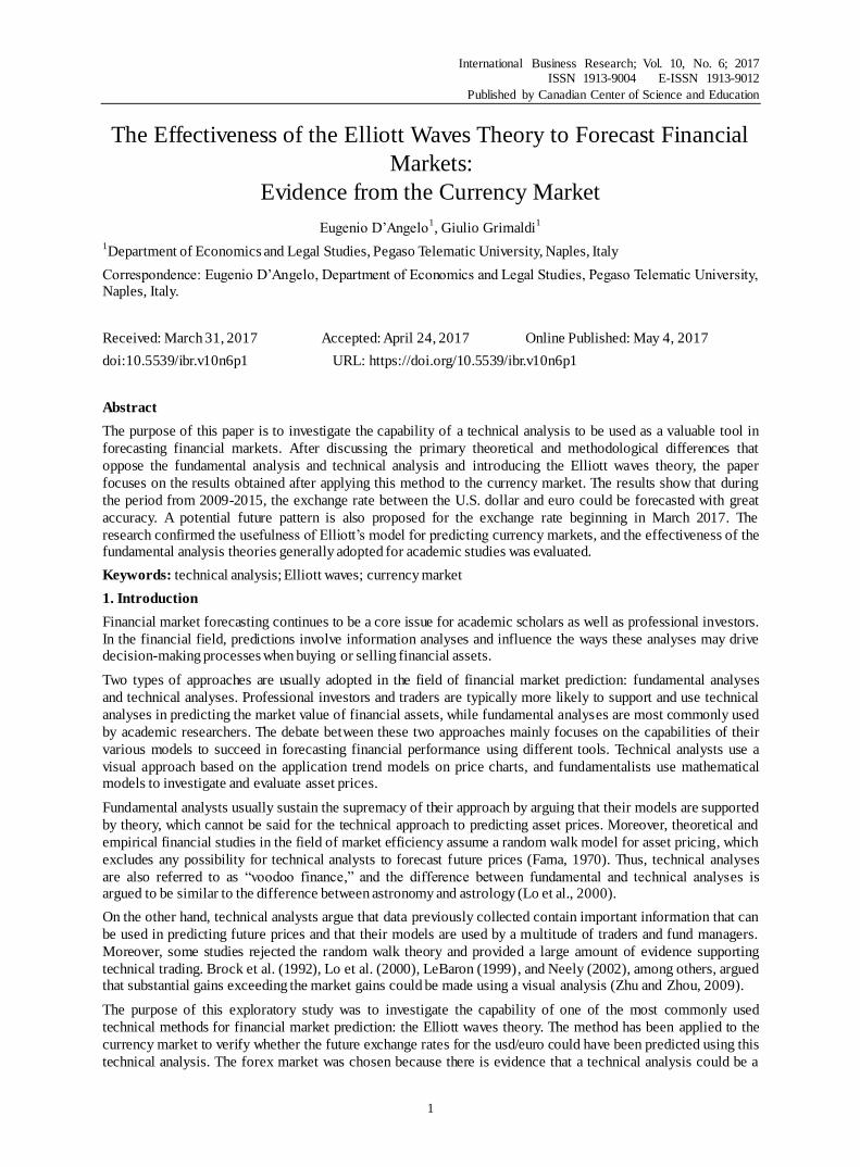
In Figure 1, the first small sequence is an impulse wave, defined as “minor” in table 1, that ends at the peak

labeled 1. This first section of the graph illustrates two indications. First, it indicates the beginning of a sequence

of three “minor” corrective waves, which will form a lower degree wave labeled 2. Second, it indicates that a wave of a higher degree, an “intermediate” wave, labeled (1), will be present in the up-trend.

Figure 1. Theoretical model of waves in an up-trend (Source: adapted from Prechter and Frost, 1978)


3

Waves 1, 2, 3, 4, and 5 are all “minor” waves and form a large impulse sequence of “intermediate” degrees, labelled (1).

As in wave 1, which is a wave of a “minor” degree, the structure of the “intermediate” impulse wave, labelled

(1), indicates two aspects. First, it predicts the beginning of a sequence of three corrective waves (a, b, and c

waves of “minor” degrees) that will form a wave of “intermediate” degree, labeled (2). Second, it suggests that the wave of a higher degree will exist in an up-trend as the a “primary” wave labelled [1].

The waves (1), (2), (3), (4), and (5) are all “intermediate” degrees and form a larger impulse wave labeled [1].

Wave [1] of the “primary” degree, as described, anticipates both the formation of an impulse wave of a “cycle”

degree in the up-trend and the formation of three corrective waves of “intermediate” degrees (a), (b), and (c), which form the wave labeled [2] of a “primary” degree.

It is important to note that at each peak of “wave one,” regardless of its degree, 1, (1), or [1], the implications are

the same. The graph in Figure 1 only shows the construction of two of the five waves that will form the “cycle” waves [1] and [2] and does not show the formation of “minute,” “minuette,” or “subminuette” sub-waves.

For the corrective waves shown in Figure 1, the waves a, c, (a), and (c) are also impulse waves of lower degrees

constituted by five sub-waves. This is because they move in the same direction of the next trend; that is,

respectively, one of the waves, (2) or (4), are “intermediate” degrees, and [2] is a “primary” degree. Waves b and

(b) are corrective waves composed of three sub-waves because they move against the wave of a higher degree, (2) and/or [2].

A simple distinction between impulse and corrective waves has been described; however, it is necessary to

provide clarification for the two types of waves. For the impulse waves, Elliott defined “motive waves” as having two categories of waves: impulses and diagonal triangles.

The most common motive wave is an impulse wave, and the main rules to be observed when labeling a wave as an impulse are as follows:

1) Wave “two” never retraces more than 100% of wave “one” of the same degree.

2) Wave “three” is never the shortest among the impulse waves (1-3-5).

3) Wave “four” never enters the territory of wave “one,” except for highly liquid markets with a very high leverage, where this condition can occur in intraday observations.

The diagonal triangle is another motive wave model, but it is not an impulse wave, as it has one or two different

characteristics. Diagonal triangles replace impulses in specific positions of a wave’s structure. As with impulses,

the corrective sub-waves do not entirely retrace the previous impulse sub-waves, and the third sub-wave is never

the shortest; however, the diagonal triangles are the only five wave structures in the direction of the main trend, where wave “four” typically overlaps wave “one.” In rare occasions, a diagonal triangle may end in a truncation.

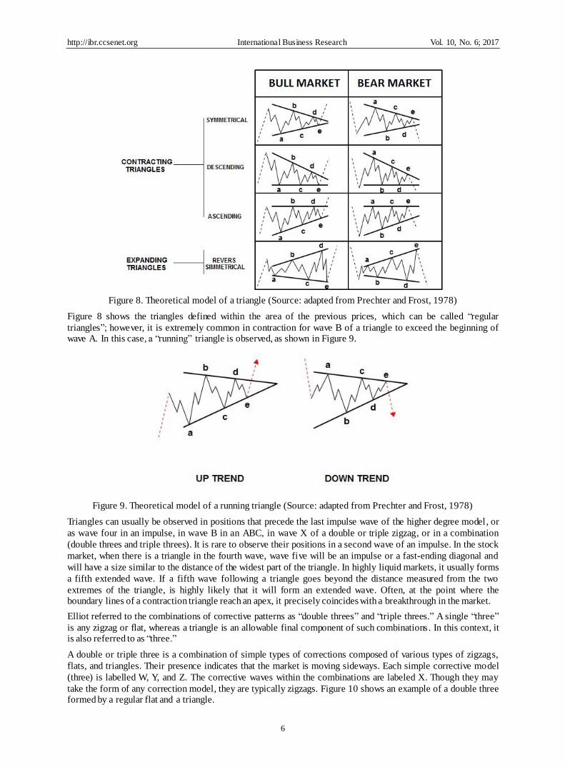
There are two types of diagonal triangles: ending diagonal and leading diagonal.

An ending diagonal is a special type of wave that occurs primarily in the fifth wave when the previous wave has

formed very quickly. Rarely, wave C, in a formation A B C, ends with this type of figure. In double or triple

threes, they appear only at the end in wave “C.” In all cases, they are located in correspondence to the end points of the larger models, indicating the end of it.

The ending diagonals have wedge shapes, where each sub-wave, including those of the waves 1, 3, and 5, is divided into “three” and not “five” waves. An example of an ending diagonal is illustrated in Figure 2.

Figure 2. Theoretical model of an ending diagonal (Source: adapted from Prechter and Frost, 1978)


4

The leading diagonal is typically formed in the impulse wave “one” and in wave “A” in corrections. The

characteristic overlapping of waves 1 and 4 and the convergence of the boundary lines of the wedge shape

remain the same as the ending diagonal; however, the subdivisions are different, forming a 5-3-5-3-5 pattern (not 3-3-3-3-3), as in Figure 3.

Figure 3. Theoretical model of a leading diagonal (Source: adapted from Prechter and Frost, 1978)

It is necessary to clarify certain aspects of corrective waves and to introduce rules to be observed when labeling

them. Corrective waves are not as easy to identify as motive waves. For this reason, an analyst should pay more

attention when the market is in a correction phase than when prices are in an impulse tendency. The most

important rule, which was derived from studying various corrective patterns, is that corrections are never

composed of five sub-waves. For this reason, an initial five-wave movement against the larger trend is never the end of a correction but only a part of it.

There are four categories of corrective models:

1) Zigzag (5-3-5; there are three types: single, double, and triple);

2) Flat (3-3-5; there are three types: regular, expanded, and running);

3) Triangles (3-3-3-3-3; there are four types: three varieties of contraction [ascending, descending, and symmetrical] and one variety of expansion [symmetrically inverse]);

4) Double threes and triple threes (combined structures).

One single zigzag in a bull market is a simple model of three bearish waves labeled A, B, and C. The sequence of

the sub-wave is 5-3-5, and the upper part of wave B is significantly lower than the beginning of wave A, as shown in Figure 4.

Figure 4. Theoretical model of a Zigzag (Source: adapted from Prechter and Frost, 1978)

A flat correction differs from a zigzag correction because the sequence of sub-waves is 3-3-5, as shown in Figure

5. In these cases, wave C generally only terminates very slightly beyond the end of wave A, unlike in the zigzags, where it ends significantly further.


5

Figure 5. Theoretical model of a regular Flat (Source: adapted from Prechter and Frost, 1978)

The variety called “expanded” is much more common, which contains an extreme price beyond the price of the

preceding impulse wave. In the expanded flat, wave B terminates beyond the starting level of wave A, and wave C ends beyond the end of wave A, as shown in Figure 6.

Figure 6. Theoretical model of an expanded flat (Source: adapted from Prechter and Frost, 1978)

A more atypical figure is the defined running flat, where wave B terminates far beyond the beginning of wave A, as in a flat expanded, but wave C is unable to cover the entire distance of A (Figure 7).

Figure 7. Theoretical model of a running flat (Source: adapted from Prechter and Frost, 1978)

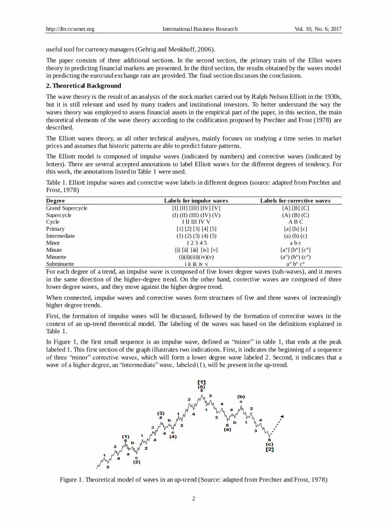
The triangles reveal a balance of forces, producing a lateral movement that is usually associated with a decrease

in volatility. The triangles contain five overlapping waves that are divided into 3-3-3-3-3 and are labeled

a-b-c-d-e. A triangle is delimited, connecting the terminal points of waves A and C and B and D. There are two

varieties of triangles: the contraction triangle and the expansion triangle. Within the range of contraction, there

are three types: symmetrical, ascending, and descending. Furthermore, there are no variations in the expanding triangle (Figure 8).


6

Figure 8. Theoretical model of a triangle (Source: adapted from Prechter and Frost, 1978)

Figure 8 shows the triangles defined within the area of the previous prices, which can be called “regular

triangles”; however, it is extremely common in contraction for wave B of a triangle to exceed the beginning of wave A. In this case, a “running” triangle is observed, as shown in Figure 9.

Figure 9. Theoretical model of a running triangle (Source: adapted from Prechter and Frost, 1978)

Triangles can usually be observed in positions that precede the last impulse wave of the higher degree model, or

as wave four in an impulse, in wave B in an ABC, in wave X of a double or triple zigzag, or in a combination

(double threes and triple threes). It is rare to observe their positions in a second wave of an impulse. In the stock

market, when there is a triangle in the fourth wave, wave five will be an impulse or a fast-ending diagonal and

will have a size similar to the distance of the widest part of the triangle. In highly liquid markets, it usually forms

a fifth extended wave. If a fifth wave following a triangle goes beyond the distance measured from the two

extremes of the triangle, is highly likely that it will form an extended wave. Often, at the point where the boundary lines of a contraction triangle reach an apex, it precisely coincides with a breakthrough in the market.

Elliot referred to the combinations of corrective patterns as “double threes” and “triple threes.” A single “three”

is any zigzag or flat, whereas a triangle is an allowable final component of such combinations. In this context, it is also referred to as “three.”

A double or triple three is a combination of simple types of corrections composed of various types of zigzags,

flats, and triangles. Their presence indicates that the market is moving sideways. Each simple corrective model

(three) is labelled W, Y, and Z. The corrective waves within the combinations are labeled X. Though they may

take the form of any correction model, they are typically zigzags. Figure 10 shows an example of a double three formed by a regular flat and a triangle.


7

Figure 10. Theoretical model of a double three (Source: adapted from Prechter and Frost, 1978)

In addition to the essential rules that govern the labeling process of motive waves and corrective waves, it is necessary to introduce guidelines that can provide further assistance in identifying the waves.

The first guideline is represented by the extension. Most impulses contain what Elliott called “extensions.”

Extensions are stretched impulses with several subdivisions. The majority of impulse waves contain an extension in one, and only one, of their three sub-waves (Figure 11).

Figure 11. Theoretical model of an extension (Source: adapted from Prechter and Frost, 1978)

The second guideline involves truncation. Elliott used the term “truncation” to describe a situation where the

fifth wave does not move passed the end of the third wave. Thus, a price pattern can be defined as a truncation

only if the fifth wave contains the necessary five sub-waves (Figure 12). The truncation often occurs due to a strong third wave.


8

Figure 12. Theoretical models of truncation (Source: adapted from Prechter and Frost, 1978)

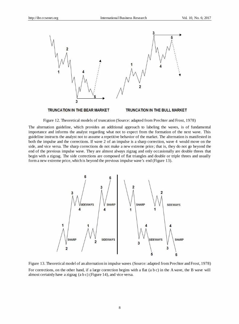
The alternation guideline, which provides an additional approach to labeling the waves, is of fundamental

importance and informs the analyst regarding what not to expect from the formation of the next wave. This

guideline instructs the analyst not to assume a repetitive behavior of the market. The alternation is manifested in

both the impulse and the corrections. If wave 2 of an impulse is a sharp correction, wave 4 would move on the

side, and vice versa. The sharp corrections do not make a new extreme price; that is, they do not go beyond the

end of the previous impulse wave. They are almost always zigzag and only occasionally are double threes that

begin with a zigzag. The side corrections are composed of flat triangles and double or triple threes and usually form a new extreme price, which is beyond the previous impulse wave’s end (Figure 13).

Figure 13. Theoretical model of an alternation in impulse waves (Source: adapted from Prechter and Frost, 1978)

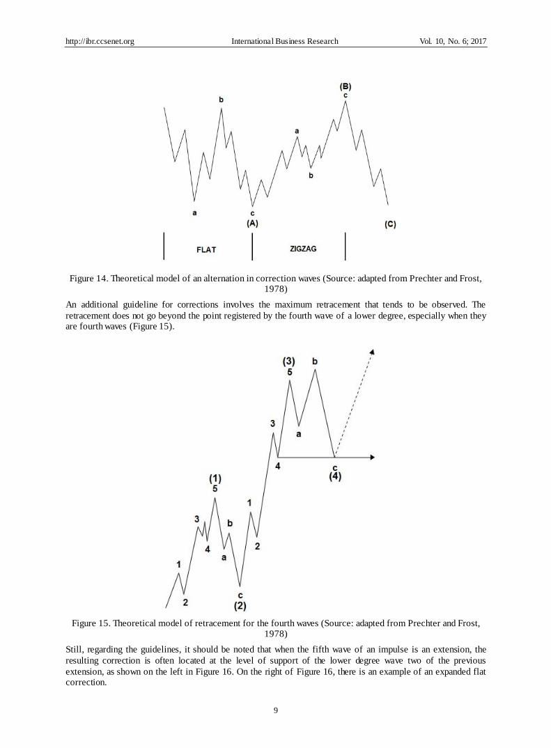
For corrections, on the other hand, if a large correction begins with a flat (a b c) in the A wave, the B wave will almost certainly have a zigzag (a b c) (Figure 14), and vice versa.


9

Figure 14. Theoretical model of an alternation in correction waves (Source: adapted from Prechter and Frost, 1978)

An additional guideline for corrections involves the maximum retracement that tends to be observed. The

retracement does not go beyond the point registered by the fourth wave of a lower degree, especially when they are fourth waves (Figure 15).

Figure 15. Theoretical model of retracement for the fourth waves (Source: adapted from Prechter and Frost, 1978)

Still, regarding the guidelines, it should be noted that when the fifth wave of an impulse is an extension, the

resulting correction is often located at the level of support of the lower degree wave two of the previous

extension, as shown on the left in Figure 16. On the right of Figure 16, there is an example of an expanded flat correction.


10

Figure 16. Theoretical model of retracement after the fifth waves (Source: adapted from Prechter and Frost, 1978)

Elliott noted that channels of parallel trends indicate the upper and lower limits of the impulse waves, often with

considerable accuracy. They are useful in determining the objectives of the waves and in providing evidence

about the future pattern. The technique used to identify the channel of an impulse wave requires at least three

peaks. By connecting the points labeled 1 and 3 and then drawing a parallel line from the point labeled 2, as shown in Figure 17, the line provides an estimated limit for wave four.

Figure 17. Theoretical model of a temporary channel (Source: adapted from Prechter and Frost, 1978)

Figure 18. Theoretical model of a definitive channel (Source: adapted from Prechter and Frost, 1978)


11

If the fourth wave ends in a point that touches the parallel line, rebuilding the channel is necessary to estimate

the movements of wave five. The channel should be drawn to connect with the end of waves 2 and 4, and if

wave 1 and wave 3 are extended, the upper parallel must begin from the peak of wave 3 to more accurately

predict the end of wave 5 (Figure 18); however, if wave 3 is extended and almost vertical, the upper parallel must begin from the top of wave 1.

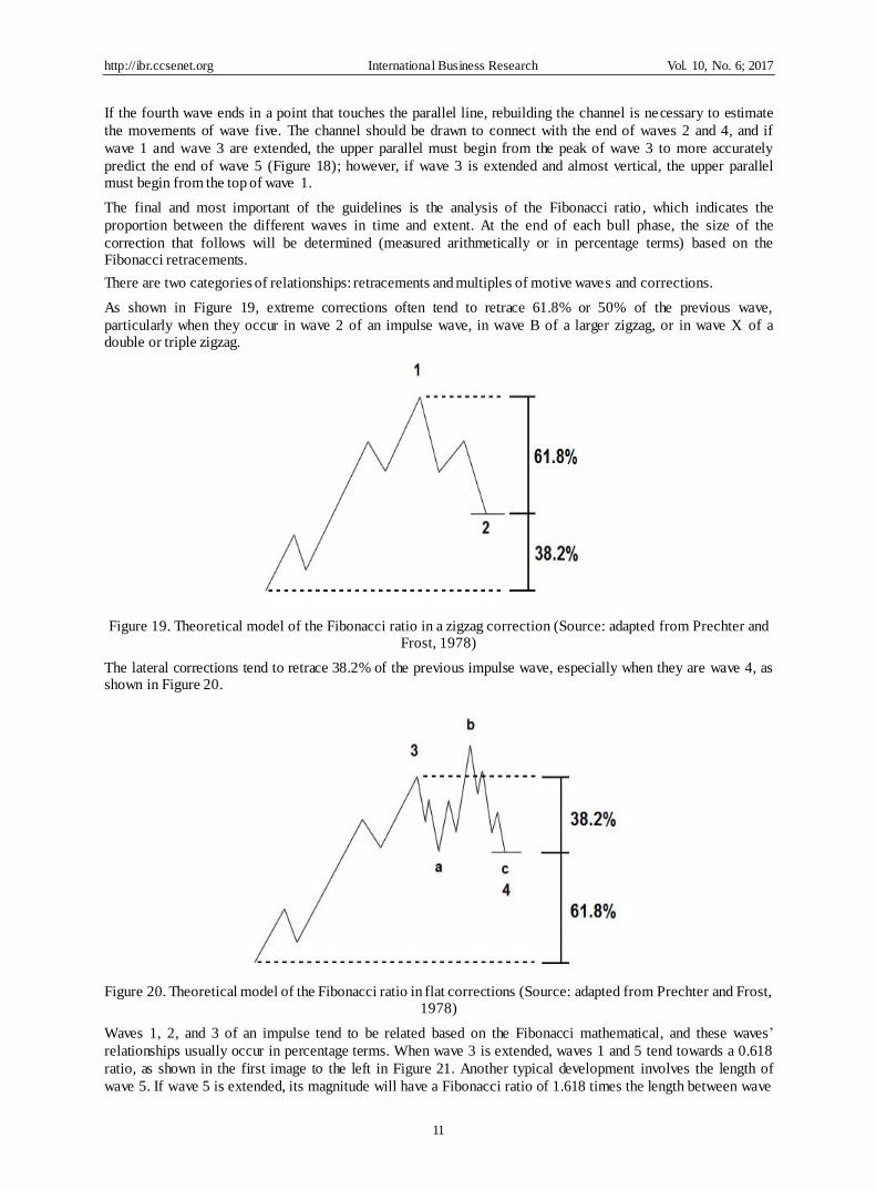
The final and most important of the guidelines is the analysis of the Fibonacci ratio, which indicates the

proportion between the different waves in time and extent. At the end of each bull phase, the size of the

correction that follows will be determined (measured arithmetically or in percentage terms) based on the Fibonacci retracements.

There are two categories of relationships: retracements and multiples of motive waves and corrections.

As shown in Figure 19, extreme corrections often tend to retrace 61.8% or 50% of the previous wave,

particularly when they occur in wave 2 of an impulse wave, in wave B of a larger zigzag, or in wave X of a double or triple zigzag.

Figure 19. Theoretical model of the Fibonacci ratio in a zigzag correction (Source: adapted from Prechter and Frost, 1978)

The lateral corrections tend to retrace 38.2% of the previous impulse wave, especially when they are wave 4, as shown in Figure 20.

Figure 20. Theoretical model of the Fibonacci ratio in flat corrections (Source: adapted from Prechter and Frost, 1978)

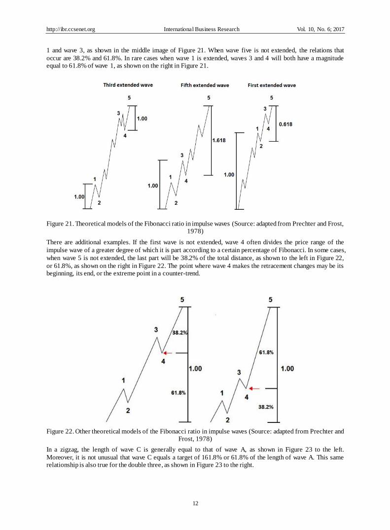
Waves 1, 2, and 3 of an impulse tend to be related based on the Fibonacci mathematical, and these waves’

relationships usually occur in percentage terms. When wave 3 is extended, waves 1 and 5 tend towards a 0.618

ratio, as shown in the first image to the left in Figure 21. Another typical development involves the length of

wave 5. If wave 5 is extended, its magnitude will have a Fibonacci ratio of 1.618 times the length between wave


12

1 and wave 3, as shown in the middle image of Figure 21. When wave five is not extended, the relations that

occur are 38.2% and 61.8%. In rare cases when wave 1 is extended, waves 3 and 4 will both have a magnitude equal to 61.8% of wave 1, as shown on the right in Figure 21.

Figure 21. Theoretical models of the Fibonacci ratio in impulse waves (Source: adapted from Prechter and Frost, 1978)

There are additional examples. If the first wave is not extended, wave 4 often divides the price range of the

impulse wave of a greater degree of which it is part according to a certain percentage of Fibonacci. In some cases,

when wave 5 is not extended, the last part will be 38.2% of the total distance, as shown to the left in Figure 22,

or 61.8%, as shown on the right in Figure 22. The point where wave 4 makes the retracement changes may be its beginning, its end, or the extreme point in a counter-trend.

Figure 22. Other theoretical models of the Fibonacci ratio in impulse waves (Source: adapted from Prechter and Frost, 1978)

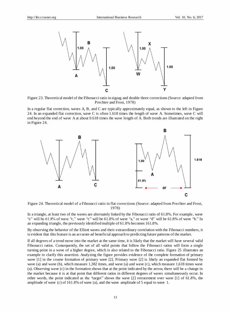
In a zigzag, the length of wave C is generally equal to that of wave A, as shown in Figure 23 to the left.

Moreover, it is not unusual that wave C equals a target of 161.8% or 61.8% of the length of wave A. This same relationship is also true for the double three, as shown in Figure 23 to the right.


13

Figure 23. Theoretical model of the Fibonacci ratio in zigzag and double three corrections (Source: adapted from Prechter and Frost, 1978)

In a regular flat correction, waves A, B, and C are typically approximately equal, as shown to the left in Figure

24. In an expanded flat correction, wave C is often 1.618 times the length of wave A. Sometimes, wave C will

end beyond the end of wave A at about 0.618 times the wave length of A. Both trends are illustrated on the right in Figure 24.

Figure 24. Theoretical model of a Fibonacci ratio in flat corrections (Source: adapted from Prechter and Frost, 1978)

In a triangle, at least two of the waves are alternately linked by the Fibonacci ratio of 61.8%. For example , wave

“e” will be 61.8% of wave “c,” wave “c” will be 61.8% of wave “a,” or wave “d” will be 61.8% of wave “b.” In an expanding triangle, the previously identified multiple of 61.8% becomes 161.8%.

By observing the behavior of the Elliott waves and their extraordinary correlation with the Fibonacci numbers, it is evident that this feature is an accurate ad beneficial approach to predicting future patterns of the market.

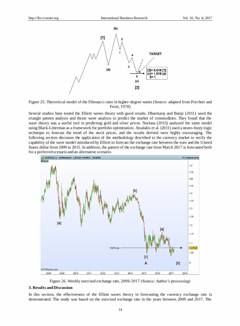
If all degrees of a trend move into the market at the same time, it is likely that the market will have several valid

Fibonacci ratios. Consequently, the set of all valid points that follow the Fibonacci ratios will form a single

turning point in a wave of a higher degree, which is also related to the Fibonacci ratio. Figure 25 illustrates an

example to clarify this assertion. Analyzing the figure provides evidence of the complete formation of primary

wave [1] in the course formation of primary wave [2]. Primary wave [2] is likely an expanded flat formed by

wave (a) and wave (b), which measure 1,382 times, and wave (a) and wave (c), which measure 1,618 times wave

(a). Observing wave (c) in the formation shows that at the point indicated by the arrow, there will be a change in

the market because it is at that point that different ratios in different degrees of waves simultaneously occur. In

other words, the point indicated as the “target” shows the wave [2] retracement over wave [1] of 61.8%, the amplitude of wave (c) of 161.8% of wave (a), and the wave amplitude of 5 equal to wave 1.


14

Figure 25. Theoretical model of the Fibonacci ratio in higher-degree waves (Source: adapted from Prechter and Frost, 1978)

Several studies have tested the Elliott waves theory with good results. Dharmaraj and Balaji (2011) used the

triangle pattern analysis and thrust wave analysis to predict the market of commodities. They found that the

wave theory was a useful tool in predicting gold and silver prices. Nurlana (2015) analyzed the same model

using Black-Litterman as a framework for portfolio optimization. Atsalakis et al. (2011) used a neuro-fuzzy logic

technique to forecast the trend of the stock prices, and the results derived were highly encouraging. The

following section discusses the application of the methodology described to the currency market to verify the

capability of the wave model introduced by Elliott to forecast the exchange rate between the euro and the United

States dollar from 2009 to 2015. In addition, the pattern of the exchange rate from March 2017 is forecasted both for a preferred scenario and an alternative scenario.

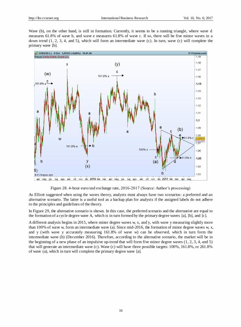
Figure 26. Weekly euro/usd exchange rate, 2009-2017 (Source: Author’s processing)

3. Results and Discussion

In this section, the effectiveness of the Elliott waves theory in forecasting the currency exchange rate is

demonstrated. The study was based on the euro/usd exchange rate in the years between 2009 and 2017. The


15

following graphs were generated using data and images taken from the ProRealTime trading platform.

In Figure 26, the formation of cycle grade wave A is shown. This wave is produced by the sub-waves [a], [b],

and [c] of a lower grade (primary grade). The pattern meets the basic rules for labeling Elliott waves, as

described in the previous section. In fact, wave [c] measures 100% of wave [a]. From 2015 to date, the market

has been in a correction phase, which should lead to the formation of a cycle grade wave B, formed by a set of three primary sub-waves, such as by wave [a] (completed) and by waves [b] and [c] (in formation).

Figure 27 highlights both the formation of the primary waves [a], [b], and [c] that form wave A of a greater

degree (cycle) as well as the formation of wave [a] (complete) and [b] (in formation), forming the cycle grade

wave B. For the formation of wave A, there is wave [a], which is a zigzag formed by the sub-waves (a), (b), and

(c) of an intermediate grade, and then wave [b], which is a running triangle formed by the sub-waves (a), (b), (c),

(d), and (e), where wave (d) measures 61.8% of wave (b) and wave (e) 61.8% of wave (c). Finally, wave [c] is

formed by the lower degree (intermediate) sub-waves (1), (2), (3), (4), and (5), where wave (3) is not the shortest

wave, and wave (5) measures 38.2% of wave (1) at the end of wave (3) beginning from the end of wave (4).

Moreover, the channel guidelines described in the previous section were met. In fact, the channel was obtained by connecting the ends of waves (2) and (4) and then by drawing the parallel line from the end of wave (3).

For wave B (in formation since 2015), on the other hand, there are waves (w), (x), and (y) of an intermediate

degree that form a primary wave [a] (double three), where wave (y) measures 100% of wave (w). Consistent

with section 2, the significance of the accuracy of the Fibonacci ratio is evident by observing the arrow in the

graph. The exchange rate is currently forming wave [b] of a primary degree, with wave (a) of an intermediate grade already completed and wave (b) in the course of formation.

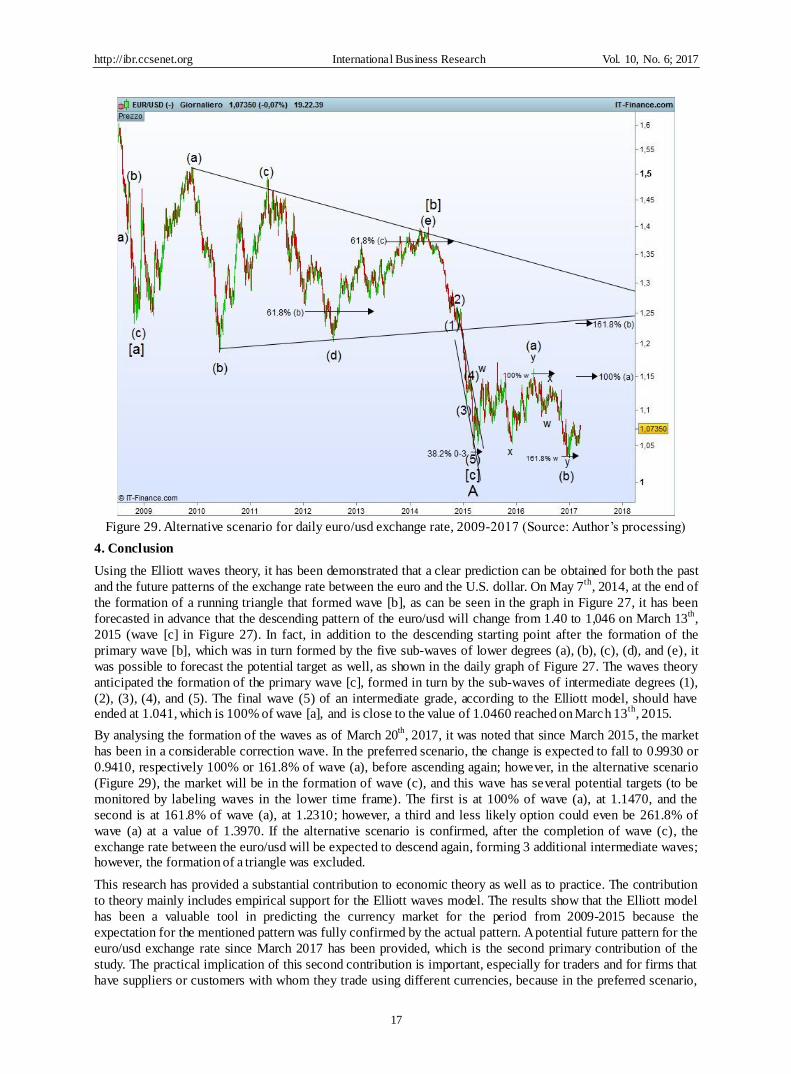
Figure 27. Daily euro/usd exchange rate, 2009-2017 (Source: Author’s processing)

In Figure 28, waves (w), (x), and (y), all of intermediate degrees, form a primary grade wave [a]. In turn, these

waves are formed by three lower grade (minor) waves. In fact, wave (w) is formed by waves a, b, and c, where

wave c is nearly 161.8% of wave a. Wave (x) is composed of waves w, x, and y, where wave y is slightly more

than 161.8% of wave w, and wave (y) is formed by the sub-waves a, b, and c, where wave c measures 161.8% of wave a with extreme precision.

Since mid-May 2016, the market has been in the formation of wave [b], where the first sub-wave (a), formed in turn by the sub-waves a, b, and c, and wave c, which measures the 100% of wave a, seems to be completed.


16

Wave (b), on the other hand, is still in formation. Currently, it seems to be a running triangle, where wave d

measures 61.8% of wave b, and wave e measures 61.8% of wave c. If so, there will be five minor waves in a

down trend (1, 2, 3, 4, and 5), which will form an intermediate wave (c). In turn, wave (c) will complete the primary wave [b].

Figure 28. 4-hour euro/usd exchange rate, 2016-2017 (Source: Author’s processing)

As Elliott suggested when using the waves theory, analysts must always have two scenarios: a preferred and an

alternative scenario. The latter is a useful tool as a backup plan for analysts if the assigned labels do not adhere to the principles and guidelines of the theory.

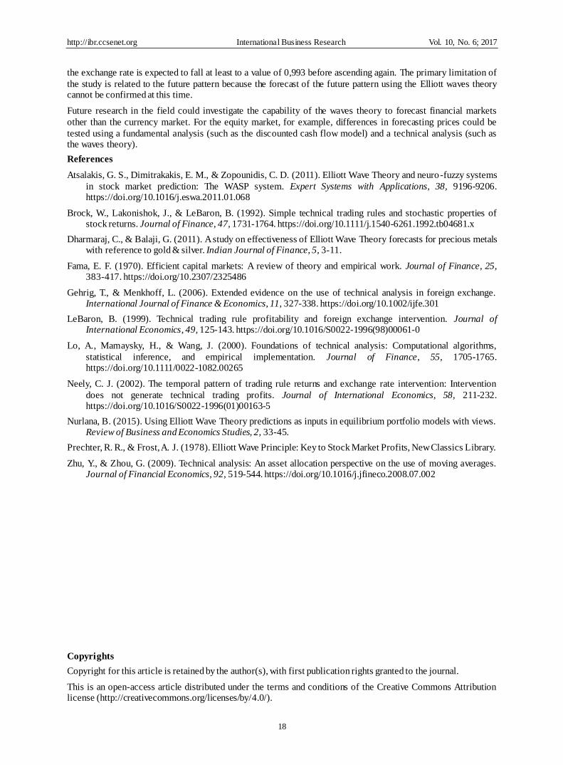
In Figure 29, the alternative scenario is shown. In this case, the preferred scenario and the alternative are equal to the formation of a cycle degree wave A, which is in turn formed by the primary degree waves [a], [b], and [c].

A different analysis begins in 2015, where minor degree waves w, x, and y, with wave y measuring slightly more

than 100% of wave w, form an intermediate wave (a). Since mid-2016, the formation of minor degree waves w, x,

and y (with wave y accurately measuring 161.8% of wave w) can be observed, which in turn form the

intermediate wave (b) (December 2016). Therefore, according to the alternative scenario, the market will be in

the beginning of a new phase of an impulsive up-trend that will form five minor degree waves (1, 2, 3, 4, and 5)

that will generate an intermediate wave (c). Wave (c) will have three possible targets: 100%, 161.8%, or 261.8% of wave (a), which in turn will complete the primary degree wave [a].


17

Figure 29. Alternative scenario for daily euro/usd exchange rate, 2009-2017 (Source: Author’s processing)

4. Conclusion

Using the Elliott waves theory, it has been demonstrated that a clear prediction can be obtained for both the past

and the future patterns of the exchange rate between the euro and the U.S. dollar. On May 7th

, 2014, at the end of

the formation of a running triangle that formed wave [b], as can be seen in the graph in Figure 27, it has been

forecasted in advance that the descending pattern of the euro/usd will change from 1.40 to 1,046 on March 13th

,

2015 (wave [c] in Figure 27). In fact, in addition to the descending starting point after the formation of the

primary wave [b], which was in turn formed by the five sub-waves of lower degrees (a), (b), (c), (d), and (e), it

was possible to forecast the potential target as well, as shown in the daily graph of Figure 27. The waves theory

anticipated the formation of the primary wave [c], formed in turn by the sub-waves of intermediate degrees (1),

(2), (3), (4), and (5). The final wave (5) of an intermediate grade, according to the Elliott model, should have ended at 1.041, which is 100% of wave [a], and is close to the value of 1.0460 reached on March 13

th, 2015.

By analysing the formation of the waves as of March 20th

, 2017, it was noted that since March 2015, the market

has been in a considerable correction wave. In the preferred scenario, the change is expected to fall to 0.9930 or

0.9410, respectively 100% or 161.8% of wave (a), before ascending again; however, in the alternative scenario

(Figure 29), the market will be in the formation of wave (c), and this wave has several potential targets (to be

monitored by labeling waves in the lower time frame). The first is at 100% of wave (a), at 1.1470, and the

second is at 161.8% of wave (a), at 1.2310; however, a third and less likely option could even be 261.8% of

wave (a) at a value of 1.3970. If the alternative scenario is confirmed, after the completion of wave (c), the

exchange rate between the euro/usd will be expected to descend again, forming 3 additional intermediate waves; however, the formation of a triangle was excluded.

This research has provided a substantial contribution to economic theory as well as to practice. The contribution

to theory mainly includes empirical support for the Elliott waves model. The results show that the Elliott model

has been a valuable tool in predicting the currency market for the period from 2009-2015 because the

expectation for the mentioned pattern was fully confirmed by the actual pattern. A potential future pattern for the

euro/usd exchange rate since March 2017 has been provided, which is the second primary contribution of the

study. The practical implication of this second contribution is important, especially for traders and for firms that

have suppliers or customers with whom they trade using different currencies, because in the preferred scenario,


18

the exchange rate is expected to fall at least to a value of 0,993 before ascending again. The primary limitation of

the study is related to the future pattern because the forecast of the future pattern using the Elliott waves theory cannot be confirmed at this time.

Future research in the field could investigate the capability of the waves theory to forecast financial markets

other than the currency market. For the equity market, for example, differences in forecasting prices could be

tested using a fundamental analysis (such as the discounted cash flow model) and a technical analysis (such as the waves theory).

References

Atsalakis, G. S., Dimitrakakis, E. M., & Zopounidis, C. D. (2011). Elliott Wave Theory and neuro-fuzzy systems

in stock market prediction: The WASP system. Expert Systems with Applications, 38, 9196-9206. https://doi.org/10.1016/j.eswa.2011.01.068

Brock, W., Lakonishok, J., & LeBaron, B. (1992). Simple technical trading rules and stochastic properties of stock returns. Journal of Finance, 47, 1731-1764. https://doi.org/10.1111/j.1540-6261.1992.tb04681.x

Dharmaraj, C., & Balaji, G. (2011). A study on effectiveness of Elliott Wave Theory forecasts for precious metals with reference to gold & silver. Indian Journal of Finance, 5, 3-11.

Fama, E. F. (1970). Efficient capital markets: A review of theory and empirical work. Journal of Finance, 25, 383-417. https://doi.org/10.2307/2325486

Gehrig, T., & Menkhoff, L. (2006). Extended evidence on the use of technical analysis in foreign exchange. International Journal of Finance & Economics, 11, 327-338. https://doi.org/10.1002/ijfe.301

LeBaron, B. (1999). Technical trading rule profitability and foreign exchange intervention. Journal of International Economics, 49, 125-143. https://doi.org/10.1016/S0022-1996(98)00061-0

Lo, A., Mamaysky, H., & Wang, J. (2000). Foundations of technical analysis: Computational algorithms,

statistical inference, and empirical implementation. Journal of Finance, 55, 1705-1765. https://doi.org/10.1111/0022-1082.00265

Neely, C. J. (2002). The temporal pattern of trading rule returns and exchange rate intervention: Intervention

does not generate technical trading profits. Journal of International Economics, 58, 211-232. https://doi.org/10.1016/S0022-1996(01)00163-5

Nurlana, B. (2015). Using Elliott Wave Theory predictions as inputs in equilibrium portfolio models with views. Review of Business and Economics Studies, 2, 33-45.

Prechter, R. R., & Frost, A. J. (1978). Elliott Wave Principle: Key to Stock Market Profits, New Classics Library.

Zhu, Y., & Zhou, G. (2009). Technical analysis: An asset allocation perspective on the use of moving averages. Journal of Financial Economics, 92, 519-544. https://doi.org/10.1016/j.jfineco.2008.07.002

Copyrights

Copyright for this article is retained by the author(s), with first publication rights granted to the journal.

This is an open-access article distributed under the terms and conditions of the Creative Commons Attribution license (http://creativecommons.org/licenses/by/4.0/).

Date post:	31-Jan-2020
Category:	Documents
Upload:	others
View:	20 times
Download:	0 times

The Effectiveness of the Elliott Waves Theory to Forecast ... · theoretical elements of the wave...

Documents