The effects of car access on employment outcomes for welfare recipients

e

es

esseeContri-rences,that caress alsoipants

iliesNF)er ap-iding

roader

e viewsServices.

Journal of Urban Economics 58 (2005) 250–272www.elsevier.com/locate/ju

The effects of car access on employment outcomfor welfare recipients✩

Tami Gurley, Donald Bruce∗

Center for Business and Economic Research and Department of Economics, 804 Volunteer Blvd.,100 Temple Court, College of Business Administration, The University of Tennessee, Knoxville, TN 37996

Received 29 September 2004; revised 26 April 2005

Available online 15 August 2005

Abstract

We use four waves of a longitudinal survey of current and former welfare recipients in Tennto examine the effects of car access on employment, weekly hours of work, and hourly wages.butions include a focus on car access instead of ownership, treatment of urban and rural diffeand controls for the simultaneity of car access and employment outcomes. Results indicateaccess generally increases the probability of being employed and leaving welfare. Car accleads to more hours of work for welfare recipients with a work requirement and enables particto find better-paying jobs. 2005 Elsevier Inc. All rights reserved.

1. Introduction

The imposition of work requirements in 1996 as part of the shift from Aid to Famwith Dependent Children (AFDC) to Temporary Assistance for Needy Families (TAmarked a major change in US welfare policy and prompted states to take a broadproach to welfare assistance. Requiring participants to work meant not only provcash assistance but also identifying and removing barriers to employment. This b

✩ This project is funded under an agreement with the Tennessee Department of Human Services. Thencompassed in this research do not necessarily reflect the views of the Tennessee Department of Human

* Corresponding author.E-mail addresses: [email protected] (T. Gurley), [email protected] (D. Bruce).

0094-1190/$ – see front matter 2005 Elsevier Inc. All rights reserved.doi:10.1016/j.jue.2005.05.002

T. Gurley, D. Bruce / Journal of Urban Economics 58 (2005) 250–272 251

ing onservicesental,

gnifi-ttle, orfor thefor arch in aate intonership

por-aneityershiphoursan and

ratherods andt of thea richpro-

ehicle

in our

re im-time

arraywork

nesseeon to a

nts andee’s gen-

. Despite. A com-arch [9])

d only acipientsower inplicable

approach was evidenced by both a change in policy and a shift toward more spendsupport services and less emphasis on cash benefits. The primary goal of supportis to remove barriers to work by providing such things as transportation, childcare, dand optical assistance.

Among barriers to work, participants consistently identify transportation as a sicant problem. Consequently, many states provide some form of reimbursement, shupublic transportation to work-related activities. States also permit asset exemptions (purposes of calculating eligibility and benefit level) either for one entire vehicle orset value amount. Researchers have argued that car ownership allows for job seabroader area, increased reliability on the job, and shorter commute times that translhigher employment rates. The recent literature has provided evidence that car owdoes indeed increase the probability of being employed.

However, previous studies suffer from a few key limitations that are potentially imtant to policy makers. First, they do not always adequately account for the simultof car ownership and employment (i.e., the idea that correlation between car ownand employment might not indicate causation) or selection bias in the estimation ofand wages. They also have not fully considered the important differences across urbrural populations. Finally, they have focused almost exclusively on car ownershipthan access. We address each of these, while also improving upon estimation methmaking use of more diverse panel data, in order to provide a more accurate accouneffects of car access on employment outcomes and welfare participation. We haveset of policy related control variables including participation in education and traininggrams. Our intent is to inform the policy debate over the relative merits of personal vsupport programs as components of a broad welfare program.

We rely on a unique panel of individual survey data from the state of Tennesseeanalysis. Tennessee’s low-income cash assistance program,Families First (FF), operatesunder a waiver from US federal guidelines. Significant features include stricter, momediate work requirements (40 hours upon entry into the program), shorter interimlimits (18 months at a time followed by three months of ineligibility), and a generousof non-cash support services (including an allowance of up to 20 hours of the weeklyrequirement for education and training activities).1

An examination of Tennessee data is useful for a number of reasons. First, Tenhas recognized the importance of automobile access for welfare recipients. In additistandard vehicle asset exemption amount, their unique benefit program,First Wheels, pro-vides zero-interest loans for the purchase of a used automobile for program participafor leavers up to 12 months after cash assistance payments end. Second, Tenness

1 For more details on program rule differences, see Center for Business and Economic Research [8]the apparent difference in policies, Tennessee’s welfare caseload is very similar to the national caseloadparison of the 2003 Families First Case Characteristics Study (Center for Business and Economic Reseand the 6th Annual Report to Congress (US Department of Health and Human Services [45]) revealefew potentially important differences. Specifically, Tennessee’s caseload has more Black and White reand fewer Hispanic recipients and recipients of other races. Average monthly TANF benefits are also lTennessee ($170 versus $355 for the US). On the whole, we view the results in this study as broadly apto other states.

252 T. Gurley, D. Bruce / Journal of Urban Economics 58 (2005) 250–272

tion atn-rurality

work-etweensation,massmightrans-andte that

ighborsm of

. First,thepoli-

stlier to-n areas.r accessarison

f thesehigh

se assetr forn states

rg and

laces the, such as

rate over

eral welfare policies closely resemble those currently being proposed for implementathe national level. Third, Tennessee data enable a more complete treatment of urbadifferences. While mostFamilies First recipients live in urban areas, a significant minorare spread across the many rural counties in the state.

2. Why car access, and how is it promoted?

Proponents argue that the lack of transportation places welfare recipients and theing poor at a disadvantage for several reasons. They note the “spatial mismatch” brural and inner-city residents and suburban employment opportunities.2 Personal vehiclemight therefore allow for a broader job search, generally more reliable transportshorter commute times, and the ability to work during hours not supported by thetransit system. A broader search area and the ability to work non-traditional hoursallow individuals to find higher paying jobs. Further, more convenient and reliable tportation is likely to increase job retention. Additional trips to day care providersretailers are also less complicated with a personal automobile. Supporters also noinner-city car ownership can lead to entrepreneurship as those with cars shuttle neon the way to jobs.3 Car ownership might also provide secondary benefits in the forstronger credit ratings.4

Those opposed to promoting car ownership also raise compelling argumentsgiven the low asset limits for eligibility, the cars available to welfare recipients andworking poor might be older or have higher mileage. This problem is exacerbated bycies that provide an asset exemption for a set value amount. Older vehicles are comaintain and emit more air pollutants than their newer counterparts.5 Further, personal vehicle promotion strategies can also lead to increased congestion, especially in urba

Despite these arguments, several states have adopted measures to facilitate caor ownership among current and former welfare recipients. Table 1 presents a compof Tennessee’s transportation-related benefits with its eight neighboring states. All ostates permit an asset exemption, ranging from a low of $1500 in Mississippi to aof the value of one vehicle in several states. Recent evidence suggests that thelimitations effect car ownership. Bansak et al. [3] find that car ownership is highefemale headed households with children in states with higher asset exemptions and i

2 For more discussion, see Ihlanfeldt and Sjoquist [23], Preston and McLafferty [37], or BlumenbeWaller [7].

3 See Davis and Johnson [13] and Cervero [10].4 Research in this area is sparse and focuses on loan or lease default rates. A study of five programs p

default rate between 2 and 7 percent and as high as 17 percent when additional criteria are consideredmaintaining employment for the duration of the payment period (Port JOBS [36]).

5 Older vehicles are subject to less stringent emission standards, and emission control systems deteriotime. For more discussion, see Barbour [4].


d

e

istance.

t laborhip.ber ofabove,pre-

exas,ms.pro-

s they

creasee of other

ncome

Table 1Transportation benefits in Tennessee and neighboring states

State Vehicle asset limit Reimbursement Bus passes Repair allowance Other

Alabama Value of one vehicle $32 per month X County specificsolutions in rural areas

Arkansas Value of one vehicle X X County specificsolutions

Georgia $4650 State: $3 per day X XCounty: $25per month

Kentucky Value of one vehicle X Regional providers andistricts providepayment and coordinattransportation

Up to $300per year

Mississippi $1500 $.20 per mile Xup to $8 per day

Missouri Value of one vehicle $5 per day

North $5000 AllowancesCarolina determined at

local level

Tennesseea $4600 $6 per dayb X XUp to $800per year

Virginia $7500 No specific Benefits paid fromoverall work programallocation

limit or cap.

Source (except Tennessee): Maiers, P., June, 1999 Transportation in Welfare Reform. Office of Family Assa Source (Tennessee): Tennessee Department of Human Services. Families First Handbook, 2000.b Reimbursement rate reduced to $4 per day as of July 1, 2003.

that exempt the value of multiple vehicles. Further, they find suggestive evidence thamarket outcomes are affected by asset limitations through their effect on car owners6

In addition to asset exemptions and the other programs listed in Table 1, a numother unique transportation benefit programs can be found in the US. As notedTennessee’sFirst Wheels program provides zero-interest loans for the purchase of aowned automobile. Wisconsin and Michigan also offer low interest loans while TMaryland, Vermont, and Colorado operate in conjunction with car donation progra7

Virginia and Ohio allow the purchase and resale of government vehicles. New Yorkvides participants with mechanical training and then allows them to purchase carhave re-conditioned.

6 Hurst and Ziliak [22] find no evidence that the increase in vehicle asset limits corresponds with an inin savings for these households. This suggests that the increase in car ownership comes at the expensinvestment in other (liquid) assets.

7 Lucas and Nicholson [28] find a positive effect of Vermont’s Good News Garage (GNG) on earned iand the probability of being employed. See their paper for more program details.


al formes is

ates—to aection 6

Em-oving

onsis-

ner-poorlyrchws.ts are

ent ofymentoun-ck ofted byn resi-

elfaret those

area.fornia.ited.ploy-

ublic,mi-, andareas

ent ofpirical

. [21],

Given that promoting car ownership has already become an important policy gomany states, understanding the impacts of these programs on employment outcovital to recognizing whether the stated objectives—namely increased employment rare likely to be met. Following a review of the prior literature in Section 3, we turndiscussion of our data and methods in Section 4. Section 5 presents results, and Sconcludes.

3. Prior research

The primary objective of TANF is to encourage self-sufficiency among recipients.ployment has been identified as a means to this end, which makes identifying and rembarriers to employment a key concern. Program participants and administrators ctently identify transportation as an important barrier to employment.8 Reasons for thetransportation difficulties are well documented. Welfare recipients often live within incity areas which are frequently isolated from suburban jobs, and they are oftenqualified for jobs in the central business district.9 Transportation also affects the job-seaarea, as many entry-level positions require applying in person for face-to-face intervie10

Transportation difficulties among current and former Tennessee welfare recipienconsistent with the literature. A 2002 study of welfare leavers found that 6.5 percunemployed leavers identified lack of adequate transportation as prohibiting emplo(Perkins and Homer [35]). Consistent with “spatial mismatch,” leavers in urban cties reported transportation difficulties more often than those in rural counties. Laa reliable car and limited public transportation were the concerns most often reporwelfare recipients; again the transportation problems were more common for urbadents (Fletcher et al. [16]; Social Work Office of Research and Public Service [43]).

A number of studies have examined the effects of labor market conditions on wdynamics. Blumenberg and Ong [5] examine access to low-wage jobs and find thawho live in areas of greater job concentration are less likely to be on welfare.11 However,even among those living in job-rich areas, most work outside of their immediate livingThis study, along with others discussed below, makes use of data from urban CaliConsequently, its applicability for policy makers in other areas may be somewhat lim

Given the above, one would expect that improved transportation might increase emment levels. Cervero et al. [11] find that among forms of transportation, private and pprivate mobility is most effective in moving participants from welfare to work. Data litations in their work, including a rather small sample size, the use of pre-TANF dataa focus on urban California residents, indicate that findings may not apply in other

8 See Blumenberg and Ong [6], Cox, et al. [12], Ebener and Klerman [14], Fein, et al. [15], Iowa DepartmHuman Services [24], Julnes and Halter [25], Owen, et al. [34], and Social Research Institute [42] for emevidence.

9 For more discussion, see Bania et al. [2], Holzer [20], Rich [40], Kain [26], Kasarda [27], Holzer et aland Stoll [44].10 See Henly [19], and Ong and McConville [33].11 Also see Ong and Blumenberg [32].


im-ture.control

nstru-ith carphaelbeennt of

r own-ce [38]failureareas

simi-that

difficul-arhethernt asrelevantr that

s.d oneas of8] andSIPP)nd thed ruralpolicy

the po-

proba-arselyur richluding

medaercent,

sampleg a carFletcherortation

address

and more recent time periods.12 However, the general association of car ownership andproved employment levels has been consistently established elsewhere in the litera13

Several studies have proceeded beyond association to causality. These studiesfor the simultaneity of the car ownership/employment decision either by using the imental variable approach or panel data. Again, the evidence is largely consistent wownership accounting for higher levels of employment (Raphael and Stoll [39]; Raand Rice [38]; Ong [31]; Cervero et al. [11]). Differences in car ownership rates haveshown to account for a portion of inter-racial employment gaps, including 43 percethe black-white differential (Raphael and Stoll [39]). Evidence also suggests that caership increases hours worked (Ong [30]; Raphael and Rice [38]). Raphael and Rifind a negative relationship between hourly wage rates and car ownership. However,to control for urban and rural differences may be driving this result as those in ruralmight be more likely to own cars and work for lower wages.

We extend the literature in a variety of ways. First, we use a transition analysislar to that of Cervero et al. [11] along with panel data to account for the possibilitybeing employed leads to car ownership or access. This approach overcomes theties of finding appropriate instrumental variables.14 In addition, instead of measuring cownership, our data provide a proxy for car access (study participants were asked wanyone in their household owned a vehicle). This distinction is potentially importahousehold members are likely to share use of a vehicle, making access at least asas ownership when considering employment benefits. In other words, it is not cleaownership would yield greater employment benefits than (the less restrictive) acces

Further, earlier work either did not control for urban and rural differences or reliea primarily urban sample. Ong [31] and Cervero et al. [11] use data from urban arLos Angeles and Alameda Counties in California, respectively. Raphael and Rice [3Raphael and Stoll [39] use national Survey of Income and Program Participation (data, however, the former study does not control for urban and rural differences, alatter focuses exclusively on 242 metropolitan areas. Our data include both urban anresidents from across the state of Tennessee. This distinction is important to statemakers as differences in transportation needs and employment opportunities affecttential benefits of a wide-scale personal vehicle promotion program.

While there is strong and consistent evidence that car ownership improves thebility of being employed, the effects of car ownership on hours and wages are spdocumented. Our analysis explores each of these employment outcomes. Finally, osurvey data permit a comparison of different samples: all survey respondents (inc

12 Cervero et al. [11] use a multinomial logit to estimate AFDC and employment transitions. Their AlaCounty, California sample consists of two points in time and 466 individuals of which only 66, or about 7 ptransition into employment.13 See Ong [30], Fletcher et al. [16], Blumenberg and Waller [7], and the references therein. Ong’sincluded four counties and consisted of 1112 observations from 1993–1994 AFDC-FC recipients. Owninincreased employment by 12 percentage points, monthly hours by 23, and monthly earnings by $152.et al. [16] used cross-sectional survey data from a 5-county area in Iowa and find positive effects of transpresources on the probability of employment and on hourly wages.14 Raphael and Stoll [39], Raphael and Rice [38], and Ong [31] use an instrumental variable approach tothe simultaneity problem.


at thement

uals

,. Those

neityin one

e. Due(18 tonalysis.with

riables

s (in-

oriesf FF,those

ns as itrdenhire

Bureaue Socialess andes of

tion orcipantsll. Noteple is not

nd localriability

data totcomes onsality or

those who had recently left the welfare rolls), those who were program participantstime of the survey, and the subset of program participants for whom a work requirewas in effect.15

4. Data and estimation procedure

Data for this analysis are taken from the first four waves of theFamily Assistance Lon-gitudinal Study (FALS).16 The respondents include a large random sample of individwho were on Tennessee’s welfare program,Families First, as of January 2001. Maximumsample sizes are 1935, 1474, 1810, and 1919 for each of the four Waves.17 In each Waveparticipants are asked whether anyone in their household owns a car or other vehicleanswering yes are assumed to have car access.

We exploit the panel nature of the FALS data in order to control for the simultaof car access and employment. Specifically, we estimate the effects of car accesswave of the survey on employment (and program participation) in a subsequent wavto the larger sample sizes in Waves 1 and 4 of the survey and the length of time24 months) between these two Waves, these two endpoints are selected for the aWhile this approach does not completely control for simultaneity, experimentationalternative estimation techniques led us to prefer it over less reliable instrumental vaapproaches.18

Multinomial logits are used to estimate the effects of Wave 1 explanatory variablecluding demographics) on the probabilities of making transitions from being onFamiliesFirst (FF) in Wave 1 to being in one of four employment and FF participation categas of the Wave 4 survey.19 These categories are unemployed/on FF, unemployed/ofemployed/on FF, and employed/off FF. Separate multinomial logits are estimated for

15 There is evidence that evaluating low-income households separately is appropriate for policy questiohas been shown that poor households respond differently to factors influencing automobile ownership (Gaand Sermons [17]).16 The FALS is an ongoing collaborative effort of the Tennessee Department of Human Services, theof Business and Economic Research/Center for Manpower Studies at the University of Memphis, and thWork Office of Research and Public Service, the Center for Literacy Studies, and the Center for BusinEconomic Research, all at the University of Tennessee in Knoxville. As of this writing, the first four wavdata were available for analysis and the sixth Wave was in the field.17 Observations from two over-sampled groups (those referred to or participating in Adult Basic EducaFamily Services Counseling) are omitted from our analysis. While a direct analysis of First Wheels partiwould be useful, sample sizes of First Wheels participants in the FALS data are unfortunately too smathat efforts were made to contact earlier-wave non-respondents in later waves. As such, the Wave 4 sama strict subset of the Wave 1 sample.18 We experimented with county-level instruments using such things as automobile insurance costs avehicle taxes, but all of our chosen instruments turned out to be quite weak due especially to lack of vawithin the state. In the absence of suitable instrumental variables, we use the panel properties of theaddress the potential simultaneity of car access and employment outcomes. Regressing employment ouprior car access status minimizes the possibility that significant results could be attributed to reverse causome common unobserved factor.19 See Green [18, pp. 720–723] for more information on multinomial logit models.


is ap-nd intotionon hours

s. Theng twoaves 1

f themmiesre) asurses,rvival

ontrolin thedingontrolBlackts in there was

urban

endixpon-4. Thewhileploy-

ectively.of thehoursre onss to awork

he issuecess and

factorsobserved

nd areavlet). The(Chat-eload.

who were unemployed in Wave 1 and those who were employed in Wave 1. Thproach allows us to assess the impact of car access on transitions off welfare aemployment.20 In addition to the multinomial logit transition analysis, Heckman selecregressions are estimated to evaluate the effects of car access and other factorsworked per week and average hourly wages.

Following Cervero et al. [11], we include three variables to measure car accesfirst indicates whether the participant had access to a car in Wave 1. The remainivariables account for the effects of gaining or losing access to a car between Wand 3.

We include a variety of control variables in all multivariate models. The age osurvey respondent is entered in quadratic form. Education variables consist of dufor less than or more than high school, with high school graduate (and nothing mothe reference category. We also include three dummies for participation in GED covocational training, and Fresh Start (a program that provides basic job market suskills). In models that are not restricted to participants with work requirements, we cfor work requirement status with an additional dummy variable. Marital status entersform of dummies for divorced (including married but separated) and committed (inclumarried, engaged, or living together), with single being the reference category. We cfor race using a series of three indicators for White, Hispanic, and other race, withserving as the reference category. We also include the number of non-caretaker adulhousehold, the dollar amount of spouse’s earnings, and a dummy for whether childcabeing provided by one of the child’s parents as control variables.21 Region-level controlsconsist of county population density, a dummy for residence in one of the four majorcounties, and the county’s unemployment rate at the time of the survey.22

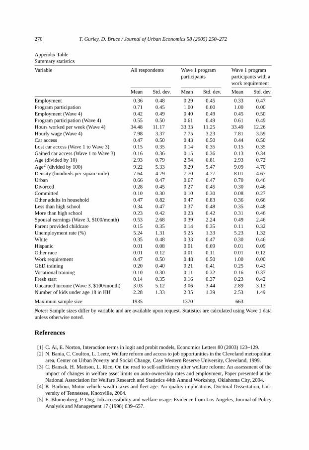
Summary statistics for all variables used in the analysis can be found in the AppTable. To highlight a few of the key variables, we first note that 36 percent of all resdents were employed as of Wave 1. This rate increases to 42 percent as of WaveWave 1 employment rate among FF participants was slightly lower at 29 percent,about one-third of those FF participants with work requirements were employed. Emment rates as of Wave 4 rose to 40 and 45 percent for these two sub-samples, respNearly three quarters of the Wave 1 respondents were participating in FF at the timeWave 1 survey, a participation rate that falls to 55 percent in Wave 4. Average weeklyof work in Wave 4 ranged from 33 to 35 for the three groups, while hourly wages wethe order of $7.75 to $8.00. Nearly half of the respondents reported having accecar in Wave 1 (43 percent of FF participants and 44 percent of FF participants with

20 Another advantage of estimating separate multinomial logits by Wave 1 employment status involves tof unobserved heterogeneity. To the extent that important factors associated both with Wave 1 car acWave 4 employment have been omitted from our specification, results could be biased. However, if thoseare correlated with Wave 1 employment then running separate models reduces the impact of the unheterogeneity.21 Due to data inavailability in earlier Waves, spouse’s earnings are taken from the Wave 3 data.22 Unemployment for June of 2002 was collected from the Bureau of Labor Statistics. Population and ladata are from the US Census Bureau, 2000 Census (http://factfinder.census.gov/servlet/BasicFactsSerfour urban counties (and the cities they contain) are Shelby (Memphis), Davidson (Nashville), Hamiltontanooga), and Knox (Knoxville). These counties account for nearly two-thirds of Tennessee’s welfare cas

http://factfinder.census.gov/servlet/BasicFactsServlet

http://factfinder.census.gov/servlet/BasicFactsServlet


aves 1

shipsresentsipantsdings:

m

nd “Off

requirements). Roughly 30 percent either lost or gained access to a car between Wand 3.

5. Results and discussion

5.1. Preliminary transition matrix analysis

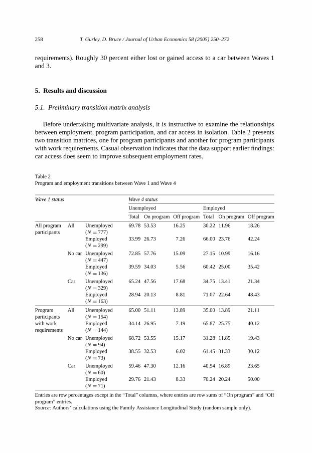
Before undertaking multivariate analysis, it is instructive to examine the relationbetween employment, program participation, and car access in isolation. Table 2 ptwo transition matrices, one for program participants and another for program particwith work requirements. Casual observation indicates that the data support earlier fincar access does seem to improve subsequent employment rates.

Table 2Program and employment transitions between Wave 1 and Wave 4

Wave 1 status Wave 4 status

Unemployed Employed

Total On program Off program Total On program Off progra

All programparticipants

All Unemployed(N = 777)

69.78 53.53 16.25 30.22 11.96 18.26

Employed(N = 299)

33.99 26.73 7.26 66.00 23.76 42.24

No car Unemployed(N = 447)

72.85 57.76 15.09 27.15 10.99 16.16

Employed(N = 136)

39.59 34.03 5.56 60.42 25.00 35.42

Car Unemployed(N = 329)

65.24 47.56 17.68 34.75 13.41 21.34

Employed(N = 163)

28.94 20.13 8.81 71.07 22.64 48.43

Programparticipantswith workrequirements

All Unemployed(N = 154)

65.00 51.11 13.89 35.00 13.89 21.11

Employed(N = 144)

34.14 26.95 7.19 65.87 25.75 40.12

No car Unemployed(N = 94)

68.72 53.55 15.17 31.28 11.85 19.43

Employed(N = 73)

38.55 32.53 6.02 61.45 31.33 30.12

Car Unemployed(N = 60)

59.46 47.30 12.16 40.54 16.89 23.65

Employed(N = 71)

29.76 21.43 8.33 70.24 20.24 50.00

Entries are row percentages except in the “Total” columns, where entries are row sums of “On program” aprogram” entries.Source: Authors’ calculations using the Family Assistance Longitudinal Study (random sample only).


ipantsrlso ap-loyed

percentpartic-

ave 1nerallyerved

m andcts oneach

ogram

ith thehaving

abilityloyedercent.sticallypants.t from

ork re-mely7 ofwork

le. Ac-ed but

ange inmended

latingram forlightly

Entries in the sixth column indicate that 16 percent of unemployed Wave 1 particwithout car access gained employment and leftFamilies First as of Wave 4. The numbewas significantly higher for those with car access, 21 percent. The difference was apreciable between employed Wave 1 program participants. Thirty-five percent of empparticipants without car access became employed and exited the program while 48of those with car access achieved the same outcome. In general, Wave 1 programipants were more likely to be employed in Wave 4 if they had access to a car in W(regardless of program participation status in Wave 4). Car access in Wave 1 also gereduced the likelihood of remaining on FF in Wave 4. These findings are also obsamong Wave 1 program participants with work requirements.

5.2. Multivariate analysis of employment and program participation

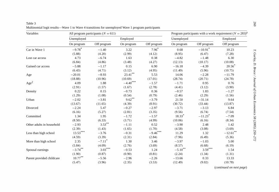
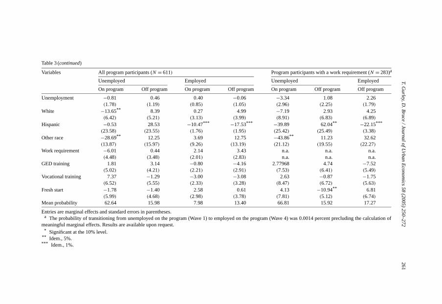
Table 3 presents results of the multinomial logit analysis for those on the prograunemployed in Wave 1. The first four columns of numbers represent marginal effethe probability of being in each of the four categories given a one-unit change inexplanatory variable, holding all other variables constant at their mean values.23 The lastthree columns present results for a sub-sample of the first group—unemployed prparticipants with a work requirement in Wave 1.24

To interpret the results in this table, consider the marginal effects associated wcar access variables in the model. Among these unemployed program participants,car access in Wave 1 decreases the probability of remaining unemployed and onFamiliesFirst by 9.78 percentage points (or about 16 percent, given that the overall probof this outcome is 62.64 percent). The increase in the probability of becoming empand leaving the program is quite substantial, 7.96 percentage points or about 59 pCar access, including gaining or losing a car between Waves 1 and 3, has no statisignificant effects on the other two transitions among the group of all program particiNote that this result pertains to all FF participants, including those who are exempwork requirements (many of whom are not able to work).

Perhaps a more relevant exercise would be to focus on those participants with wquirements. After all, vehicle supports are typically intended to help participants—nathose required to work—achieve self-sufficiency more quickly. Columns 5 throughTable 3 restrict the analysis to the group of unemployed program participants withrequirements.

There are two statistically significant effects of car access among this sub-sampcess to a car in Wave 1 dramatically reduces the probability of remaining unemploy

23 For dummy variables, the marginal effect represents the change in the particular probability given a chthe dummy variable from 0 to 1. Note the marginal effect of age-squared has not been adjusted as recomin Ai and Norton [1] and Norton et al. [29].24 The data were adequate for estimating the multinomial logit model but were not sufficient for calcumarginal effects for the transition from unemployed and on the program to employed and on the progWave 1 participants with a work requirement (the estimated probability of making this transition was just sgreater than zero).

260T.G

urley,D.B

ruce/JournalofU

rbanE

conomics

58(2005)

250–272Table 3Multinomial logit results—Wave 1 to Wave 4 transitions for unemployed Wave 1 program participants

rogram participants with a work requirement (N = 283)a

Unemployed Employed

On program Off program Off program

0.68 −10.91* 10.23(8.95) (6.47) (7.28)−4.82 −1.48 6.30

(12.13) (10.17) (10.08)−16.18 −4.39 20.56*

(11.49) (5.96) (10.75)14.06 −2.28 −11.79

(28.74) (20.71) (24.78)−1.71 0.95 0.76(4.41) (3.12) (3.90)−0.57 1.83 −1.27(2.46) (2.29) (1.56)21.50 −31.14 9.64

(30.72) (33.44) (13.87)−3.71 −3.13 6.84(9.56) (6.74) (7.54)18.33* −11.23* −7.09

(10.06) (6.16) (8.34)−3.90 2.48 1.42(4.58) (3.08) (3.69)11.29 1.32 −12.61**

(7.96) (6.49) (5.36)−3.97 −1.03 5.00(8.57) (6.68) (6.19)−5.10** 3.59*** 1.54(2.24) (1.34) (1.31)

−13.66 0.33 13.33(12.49) (9.02) (10.78)

(continued on next page)

Variables All program participants (N = 611)

Unemployed Employed

On program Off program On program Off program

Car in Wave 1 −9.78* −1.40 3.22 7.96*

(5.88) (4.20) (2.99) (4.12)Lost car access 4.73 −6.74 1.63 0.38

(6.84) (4.86) (3.48) (4.27)Gained car access −5.88 −1.17 0.15 6.90

(6.43) (4.71) (3.12) (4.95)Age −20.01 −8.93 23.41** 5.53

(18.88) (10.96) (10.69) (17.01)Age2 4.09 1.88 −4.40*** −1.57

(2.91) (1.57) (1.67) (2.78)Density 0.22 0.15 −0.73 0.36

(1.29) (1.08) (0.54) (0.79)Urban −2.02 −3.81 9.62** −3.79

(13.67) (11.65) (4.39) (8.91)Divorced −2.24 5.47 −0.27 −2.97

(6.16) (5.27) (2.81) (3.35)Committed 1.34 1.95 −1.72 −1.57

(8.50) (6.33) (3.71) (4.99)Other adults in household −2.93 3.53** −1.11 0.52

(2.39) (1.43) (1.65) (1.70)Less than high school 13.53*** −3.76 −0.31 −9.46***

(4.59) (3.39) (2.31) (2.84)More than high school 2.35 −7.11* 1.30 3.46

(5.84) (4.09) (2.76) (3.69)Spousal earnings −3.74** 3.03*** −0.53 1.24

(1.90) (0.87) (0.90) (0.81)Parent provided childcare 10.77** −5.56 −2.96 −2.26

(5.47) (3.96) (2.35) (3.53)

P

T.Gurley,D

.Bruce

/JournalofUrban

Econom

ics58

(2005)250–272

261


Unemployed Employed

On program Off program Off program

−3.34 1.08 2.26(2.96) (2.25) (1.79)−7.19 2.93 4.25(8.91) (6.83) (6.89)

−39.89 62.04** −22.15***

(25.42) (25.49) (3.38)−43.86** 11.23 32.62(21.12) (19.55) (22.27)

n.a. n.a. n.a.n.a. n.a. n.a.

2.77968 4.74 −7.52(7.53) (6.41) (5.49)

2.63 −0.87 −1.75(8.47) (6.72) (5.63)

4.13 −10.94** 6.81(7.81) (5.12) (6.74)66.81 15.92 17.27

gram (Wave 4) was 0.0014 percent precluding the calculation of

Table 3 (continued)

Variables All program participants (N = 611) P

Unemployed Employed


Unemployment −0.81 0.46 0.40 −0.06(1.78) (1.19) (0.85) (1.05)

White −13.65** 8.39 0.27 4.99(6.42) (5.21) (3.13) (3.99)

Hispanic −0.53 28.53 −10.47*** −17.53***

(23.58) (23.55) (1.76) (1.95)Other race −28.69** 12.25 3.69 12.75

(13.87) (15.97) (9.26) (13.19)Work requirement −6.01 0.44 2.14 3.43

(4.48) (3.48) (2.01) (2.83)GED training 1.81 3.14 −0.80 −4.16

(5.02) (4.21) (2.21) (2.91)Vocational training 7.37 −1.29 −3.00 −3.08

(6.52) (5.55) (2.33) (3.28)Fresh start −1.78 −1.40 2.58 0.61

(5.99) (4.68) (2.98) (3.78)Mean probability 62.64 15.98 7.98 13.40

Entries are marginal effects and standard errors in parentheses.a The probability of transitioning from unemployed on the program (Wave 1) to employed on the pro

meaningful marginal effects. Results are available upon request.* Significant at the 10% level.

** Idem., 5%.*** Idem., 1%.


g em-Whilents,

evant

loyedabilityts (88m by1 pro-riesnious

ragingonly

tatusthataccessnot

vari-ectedor re-onswho

higher4 and

aves 1nge inoverty

interac-upon

lose itble forservedges suchnds that

d that

moving off the program (by 10.91 percentage points, or about 69 percent).25 Gaining caraccess between Waves 1 and 3 of the survey increases the probability of becomiployed and leaving the program by 20.56 percentage points or over 100 percent.results differ from those in Columns 1 through 4 for all unemployed program participit is refreshing to find that car access has positive impacts on the more policy-resub-sample of those with work requirements.

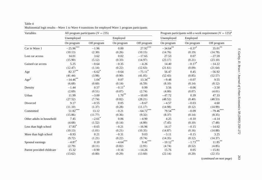
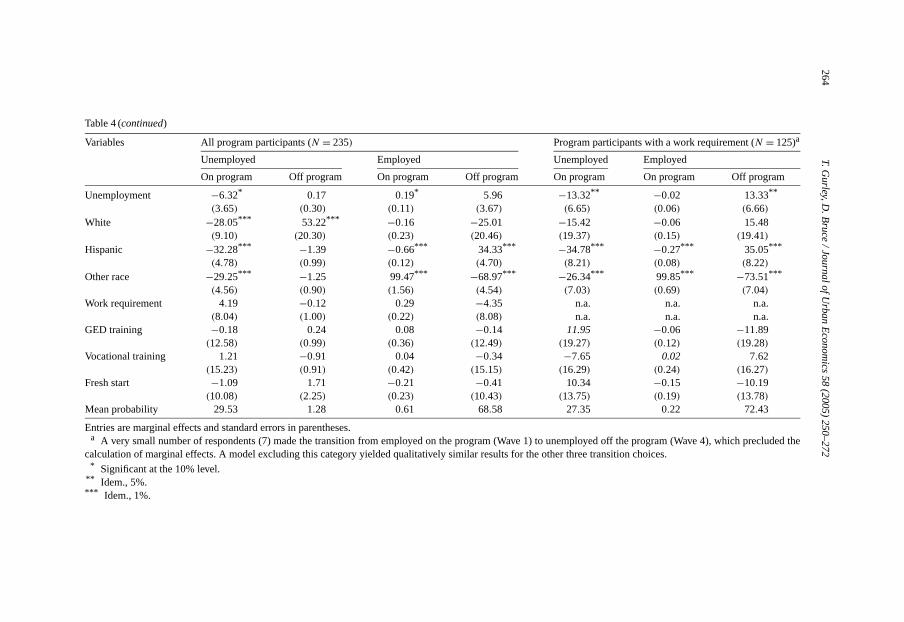
The analysis in Table 3 was duplicated for those who were on the program andemployedin Wave 1, and results are presented in the same format in Table 4. Among all emprogram participants in Wave 1, having access to a car in Wave 1 reduced the probof becoming unemployed while remaining on the program by 25.96 percentage poinpercent) and increased the probability of remaining employed but leaving the progr27.92 percentage points (41 percent). Restricting the analysis to employed Wavegram participants with work requirements, we find similar but larger effects. In a sof robustness checks, the car effects remained virtually unchanged in more parsimmodels and were robust to the omission of urban and rural controls.26 Overall, the resultsare consistent and indicate large and significant benefits from car access in encoself-sufficiency through employment. These findings are generally in line with theother similar study in the literature (Cervero et al. [11]).

It is interesting that most of the identified car access effects are from the Wave 1indicator rather than the “lost” and “gained” indicators. The interpretation of this ishaving access to a car in Wave 1 outweighs the negative consequences of losing thaby Wave 3. Similarly, the negative effects of not having car access in Wave 1 artypically offset by a positive bonus from gaining access by Wave 3.27

Effects of other explanatory variables exhibited a few general patterns. Educatioables, when significant, affected employment and program participation in the expmanner. Respondents in committed relationships were much less likely to becomemain employed and exit welfare.28 The effects of spousal earnings suggest that the permost likely to become or remain employed and leave the program select partnerare also more likely to experience positive outcomes. Respondents who reportedspousal earnings were less likely to be unemployed and on the program as of Wav

25 In this case, Wave 1 car access might be signaling the absence of other major life changes betweenand 4. Those recipients who remained unemployed but left welfare were more likely to experience a chmarital status or a change in the number of adults in the household, and less likely to transition out ofbetween Waves 1 and 4.26 We also experimented with an interaction between Wave 1 car access and the urban dummy. Thistion was never statistically significant in the multinomial logits. Full results are available from the authorsrequest.27 This is not an outgrowth of small sample sizes as about one-third of those with car access in Waveby Wave 3 and a similar share of those without Wave 1 access gain it by Wave 3 (see the Appendix Tdetails). To be sure, the lack of a significant effect from the lost or gained variables could be due to unoheterogeneity (as discussed above). It is also possible that a change in car access signals other life chaas a move or change in marital status that mitigate the expected car effects. For example, a recent studychanges in marital status affect employment outcomes (Richards and Bruce [41]).28 This echoes our earlier study on marriage impacts. Using a similar set of control variables, we fourespondents married in both Waves 1 and 3 of the survey were significantlyless likely to be employed in Wave 4than those who were unmarried in both of these earlier waves (Richards and Bruce [41]).

n

al

p

a

eo

u

s

te

n

ss

e

Wap

1abnfi

n

T.Gurley,D

.Bruce

/JournalofUrban

Econom

ics58

(2005)250–272

263Table 4Multinomial logit results—Wave 1 to Wave 4 transitions for employed Wave 1 program participants


Unemployed Employed

On program On program Off program

−34.64** −0.37* 35.01**

(14.76) (0.19) (14.78)27.53 0.07 −27.59

(23.17) (0.21) (23.10)14.40 −0.17* −14.22

(21.61) (0.09) (21.64)56.47 0.45 −56.92

(52.43) (0.85) (52.57)−9.48 −0.07 9.55(8.10) (0.14) (8.12)

3.56 −0.06 −3.50(4.00) (0.07) (4.01)

−47.72 0.39 47.33(48.52) (0.40) (48.53)−4.57 −0.03 4.60

(14.98) (0.12) (14.99)79.54*** −0.09 −79.46***

(8.37) (0.14) (8.35)4.25 −0.10 −4.14

(7.45) (0.10) (7.48)14.17 −0.15 −14.02

(14.87) (0.16) (14.88)−3.11 −0.15 3.25

(14.35) (0.12) (14.37)−10.12** −1.73*** 11.85**

(4.74) (0.52) (4.85)15.76 0.05 −15.81

(22.14) (0.20) (22.15)

(continued on next page)

Variables All program participants (N = 235) P

Unemployed Employed


Car in Wave 1 −25.96*** −1.96 0.00 27.92***

(10.13) (2.30) (0.26) (10.15)Lost car access 14.01 3.62 0.02 −17.65

(15.90) (5.12) (0.33) (14.97)Gained car access 5.25 −0.64 −0.35 −4.26

(12.47) (1.14) (0.22) (12.63)Age 82.37** −6.62* −0.64 −75.11*

(41.44) (3.98) (0.90) (41.05)Age2 −14.46** 1.04* 0.07 13.34**

(6.68) (0.60) (0.14) (6.59)Density −1.44 0.57 −0.11* 0.99

(2.69) (0.51) (0.07) (2.74)Urban 11.99 −3.00 1.70** −10.69

(27.52) (7.74) (0.82) (28.21)Divorced 9.17 −0.55 0.05 −8.67

(11.10) (1.37) (0.28) (11.17)Committed 51.82*** 13.12 −0.21 −64.72***

(15.86) (11.77) (0.36) (9.32)Other adults in household 7.45 −2.61* 0.06 −4.90

(4.68) (1.52) (0.14) (4.80)Less than high school 17.83* −0.65 −0.21 −16.96

(10.13) (1.01) (0.21) (10.35)More than high school −8.93 0.21 −0.31 9.03

(9.72) (1.21) (0.22) (9.74)Spousal earnings −4.87* 0.10 −4.64*** 9.41***

(2.79) (0.11) (0.82) (2.91)Parent provided childcare 15.32 −0.90 −0.16 −14.26

(13.62) (0.80) (0.29) (13.60)

264T.G

urley,D.B

ruce/JournalofU

rbanE

conomics

58(2005)

250–272

Program participants with a work requirement (N = 125)a

Unemployed Employed

On program On program Off program

−13.32** −0.02 13.33**

(6.65) (0.06) (6.66)−15.42 −0.06 15.48(19.37) (0.15) (19.41)−34.78*** −0.27*** 35.05***

(8.21) (0.08) (8.22)−26.34*** 99.85*** −73.51***

(7.03) (0.69) (7.04)n.a. n.a. n.a.n.a. n.a. n.a.

11.95 −0.06 −11.89(19.27) (0.12) (19.28)−7.65 0.02 7.62

(16.29) (0.24) (16.27)10.34 −0.15 −10.19

(13.75) (0.19) (13.78)27.35 0.22 72.43

e 1) to unemployed off the program (Wave 4), which precludedthethe other three transition choices.

Table 4 (continued)

Variables All program participants (N = 235)

Unemployed Employed


Unemployment −6.32* 0.17 0.19* 5.96(3.65) (0.30) (0.11) (3.67)

White −28.05*** 53.22*** −0.16 −25.01(9.10) (20.30) (0.23) (20.46)

Hispanic −32.28*** −1.39 −0.66*** 34.33***

(4.78) (0.99) (0.12) (4.70)Other race −29.25*** −1.25 99.47*** −68.97***

(4.56) (0.90) (1.56) (4.54)Work requirement 4.19 −0.12 0.29 −4.35

(8.04) (1.00) (0.22) (8.08)GED training −0.18 0.24 0.08 −0.14

(12.58) (0.99) (0.36) (12.49)Vocational training 1.21 −0.91 0.04 −0.34

(15.23) (0.91) (0.42) (15.15)Fresh start −1.09 1.71 −0.21 −0.41

(10.08) (2.25) (0.23) (10.43)Mean probability 29.53 1.28 0.61 68.58

Entries are marginal effects and standard errors in parentheses.a A very small number of respondents (7) made the transition from employed on the program (Wav

calculation of marginal effects. A model excluding this category yielded qualitatively similar results for* Significant at the 10% level.

** Idem., 5%.*** Idem., 1%.


xit the

ed peredingpants,e mostwever,ar be-.more

nabil-a car

acter-idenceailable

1 caract, the.06 for

Wave 4gh carto find

lusion

rved forld’s un-. Results

].n Wave 4percent),

ajority oft full-timeand 39

ing more

milton,ultaneityminimizedesidence

respondents employed as of Wave 1 were more likely to remain employed and eprogram as of Wave 4 the higher their reported spousal earnings.

5.3. Multivariate analysis of weekly hours worked and average hourly earnings

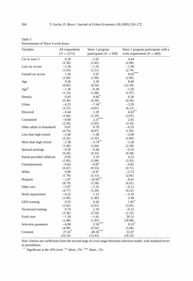
Table 5 presents the results from Heckman selection regressions of hours workweek in Wave 4.29 Explanatory variables remain the same as those in the precmultinomial logit analyses, and results for all study respondents, program particiand program participants with a work requirement are presented separately. For thpart, car access does not seem to be an important determinant of work hours. Hoamong Wave 1 program participants with work requirements, gaining access to a ctween Waves 1 and 3 increases work hours in Wave 4 by nearly 9 hours per week30 Aswith our analysis of employment, effects of the car variables remained consistent inparsimonious models and were robust to exclusion of urban control variables.

The lack of a strong effect of car access overall may be indicative of a general iity among the samples in question to alter their hours of work. Having access tomight increase one’s ability to find and keep a job, but the jobs are likely to be charized by standard labor hours contracts (e.g., with a 40-hour work week). Survey evadds credence to this contention that employers generally offered a limited set of avhours.31

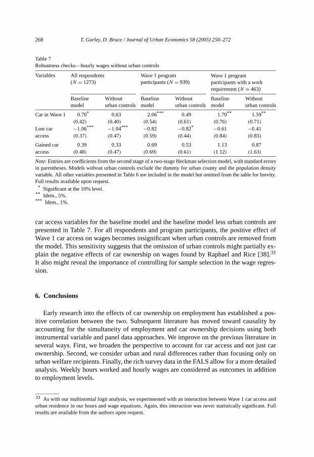
Regression results for hourly wages are reported in Table 6. We find that Waveaccess increases Wave 4 average hourly wages for all three of our samples. In fincreases are quite large, ranging from $0.70 per hour for all respondents to $2Wave 1 program participants. Losing car access between Waves 1 and 3 reduces thewage by slightly more than one dollar per hour among all respondents. Even thouaccess has little to no effect on hours of work, it does seem to enable respondentsbetter-paying jobs.

Interestingly, the effects of car access on hourly wages are sensitive to the incof urban control variables, at least for the more inclusive samples.32 Coefficients for the

29 We employ a two-stage selection model to account for the fact that hours and wages are only obseworking respondents. The identification variables for the first-stage employment probit are the househoearned income (as of Wave 3) and the number of children under age 18 in the household (as of Wave 1)from first-stage probits are available upon request.30 This magnitude may seem large, but it echoes similar findings by Ong [30] and Raphael and Rice [3831 Participants were asked how many hours per week they usually worked. The most frequent response iwas 40 hours per week (34 percent). Other common responses were 20 hours (7 percent), 30 hours (935 hours (9 percent), and 50 hours (3 percent). The average number of hours worked was 34 and the mrespondents reported that they usually worked less than 40 hours per week (54 percent) suggesting thaemployment opportunities might have been limited. Fifteen percent worked 20 or fewer hours per weekpercent worked between 20 and 39 hours per week. Twelve percent of the respondents reported workthan 40 hours per week.32 Urban control variables include a dummy variable for residence in an urban county (Davidson, HaKnox, and Shelby) and a variable for population density. To be sure, we have not addressed potential simbetween car access and urban residence. Since both enter our models as Wave 1 values, we haveproblems of simultaneity with employment outcomes. Relationships between car access and urban rvariables will only have the usual multicollinearity consequences of inflating standard errors.


d errors

Table 5Determinants of Wave 4 work hours

Variables All respondents(N = 1273)

Wave 1 programparticipants (N = 939)

Wave 1 program participants withwork requirement (N = 460)

Car in wave 1 0.18 −1.65 4.44(2.36) (2.45) (2.96)

Lost car access −2.30 −1.32 −1.96(1.63) (2.11) (2.74)

Gained car access 1.30 2.07 8.65***

(1.69) (1.99) (2.96)Age 9.56 3.18 8.40

(6.82) (6.54) (12.30)Age2 −1.30 −0.38 −1.92

(1.14) (1.08) (1.97)Density 0.45 0.66* 0.26

(0.30) (0.39) (0.56)Urban −4.23 −7.34* −3.29

(3.15) (4.01) (6.13)Divorced −0.44 1.20 6.02**

(1.66) (2.10) (3.01)Committed −0.80 2.37*** 2.81

(2.26) (2.95) (3.35)Other adults in household 0.01 0.78 −0.35

(0.74) (0.97) (1.92)Less than high school −2.40 −1.38 −2.69

(2.22) (2.32) (2.60)More than high school −2.38 −3.74** −3.28

(1.49) (1.64) (2.58)Spousal earnings −0.20 −0.44 −0.16

(0.20) (0.33) (0.38)Parent provided childcare 0.92 3.19 4.52

(1.85) (2.08) (2.92)Unemployment −0.63 −0.87 −0.81

(0.47) (0.53) (0.71)White 0.80 −0.47 −2.72

(1.78) (2.15) (2.81)Hispanic −1.97 −10.93** −8.41

(8.79) (5.58) (6.91)Other race −5.97 −5.32 −6.11

(4.77) (5.26) (6.22)Work requirement −0.22 1.13 −4.19

(1.06) (1.40) 2.49GED training 0.55 0.26 1.81*

(1.65) (2.01) (3.05)Vocational training 0.74 2.19 −0.15

(2.36) (2.54) (2.22)Fresh start −1.39 −1.61 20.31

(1.48) (1.93) (18.98)Selection parameter −6.98 2.56*** 8.33*

(4.99) (0.16) (5.06)Constant 27.41* 40.36*** 22.07

(16.16) (13.43) (18.33)

Note: Entries are coefficients from the second stage of a two-stage Heckman selection model, with standain parentheses.

* Significant at the 10% level.∗∗ Idem., 5%.∗∗∗ Idem., 1%.

a

r


a

rd errors

Table 6Determinants of Wave 4 hourly wages



Wave 1 program participants withwork requirement (N = 463)

Car in Wave 1 0.70* 2.06*** 1.70**

(0.42) (0.54) (0.76)Lost car access −1.06*** −0.82 −0.61

(0.37) (0.59) (0.84)Gained car access 0.39 0.69 1.13

(0.48) (0.69) (1.12)Age 1.79* 2.09 2.12

(1.04) (1.90) (4.14)Age2 −0.24 −0.43 −0.43

(0.15) (0.29) (0.61)Density 0.14 0.12 −0.20

(0.09) (0.12) (0.18)Urban −1.15 −0.69 3.10*

(0.84) (1.26) (1.86)Divorced −0.38 −0.09 0.89

(0.37) (0.56) (0.80)Committed 0.04 −1.20 −0.97

(0.50) (0.88) (1.28)Other adults in household 0.05 −0.39 −0.69

(0.22) (0.31) (0.63)Less than high school −0.50 −1.43*** −1.81**

(0.41) (0.45) (0.80)More than high school 1.33*** 1.47*** 1.09

(0.34) (0.52) (0.70)Spousal earnings −0.03 −0.11 −0.08

(0.05) (0.08) (0.09)Parent provided childcare −0.83*** −1.02* −0.22

(0.30) (0.61) (0.93)Unemployment 0.08 0.23 0.55**

(0.11) (0.16) (0.27)White −0.46 −0.47 −0.27

(0.51) (0.66) (1.03)Hispanic 0.15 −0.70 0.32

(0.90) (2.47) (3.01)Other race 0.30 0.90 2.00

(0.72) (1.14) (1.56)Work requirement 0.18 0.40 n.a.

(0.26) (0.40) n.a.GED training −0.06 −0.49 n.a.

(0.44) (0.57) n.a.Vocational training 0.00 −0.82 n.a.

(0.58) (0.66) n.a.Fresh start 0.19 0.71 1.23*

(0.37) (0.52) (0.75)Selection parameter −0.25 4.68*** 5.15***

(0.45) (0.64) (0.89)Constant 4.05** −1.28 −3.69

(1.88) (3.32) (8.14)

Note: Entries are coefficients from the second stage of a two-stage Heckman selection model, with standain parentheses.

* Significant at the 10% level.∗∗ Idem., 5%.∗∗∗ Idem., 1%.


rd errorsdensityrevity.

trols areffect ofed fromlly ex-[38].gres-

a pos-lity byboth

ture injust carnly on

tailedddition

ss andant. Full

Table 7Robustness checks—hourly wages without urban controls



Wave 1 programparticipants with a workrequirement (N = 463)

Baselinemodel

Withouturban controls

Baselinemodel


Baselinemodel


Car in Wave 1 0.70* 0.63 2.06*** 0.49 1.70** 1.59**

(0.42) (0.40) (0.54) (0.61) (0.76) (0.71)Lost car −1.06*** −1.04*** −0.82 −0.82* −0.61 −0.41access (0.37) (0.47) (0.59) (0.44) (0.84) (0.83)

Gained car 0.39 0.33 0.69 0.53 1.13 0.87access (0.48) (0.47) (0.69) (0.61) (1.12) (1.63)

Note: Entries are coefficients from the second stage of a two-stage Heckman selection model, with standain parentheses. Models without urban controls exclude the dummy for urban county and the populationvariable. All other variables presented in Table 6 are included in the model but omitted from the table for bFull results available upon request.

* Significant at the 10% level.** Idem., 5%.*** Idem., 1%.

car access variables for the baseline model and the baseline model less urban conpresented in Table 7. For all respondents and program participants, the positive eWave 1 car access on wages becomes insignificant when urban controls are removthe model. This sensitivity suggests that the omission of urban controls might partiaplain the negative effects of car ownership on wages found by Raphael and Rice33

It also might reveal the importance of controlling for sample selection in the wage resion.

6. Conclusions

Early research into the effects of car ownership on employment has establisheditive correlation between the two. Subsequent literature has moved toward causaaccounting for the simultaneity of employment and car ownership decisions usinginstrumental variable and panel data approaches. We improve on the previous literaseveral ways. First, we broaden the perspective to account for car access and notownership. Second, we consider urban and rural differences rather than focusing ourban welfare recipients. Finally, the rich survey data in the FALS allow for a more deanalysis. Weekly hours worked and hourly wages are considered as outcomes in ato employment levels.

33 As with our multinomial logit analysis, we experimented with an interaction between Wave 1 car acceurban residence in our hours and wage equations. Again, this interaction was never statistically significresults are available from the authors upon request.


e firstogramogram

1 are4. Re-orkbabilityod ofr em-

urs forcreasesipantsr-payingave 1.

ing aearliermarketly.ovingar ac-

ublicwages.weeklyhaveagescome

an-e thethe ef-

lysis ofemploy-

ymousatisticsity of

fts.

Our results are broadly consistent with those of earlier work. Our analysis ofunem-ployed Wave 1 program participants reveals that those who had car access in thwave of the survey are much more likely to become employed and leave the pras of Wave 4 (18–24 months later). Among the subset of unemployed Wave 1 prparticipants who had work requirements, those who had access to a car in Wavedramatically less likely to remain unemployed and leave the program as of Wavesults are similar in spirit foremployed Wave 1 program participants, regardless of wrequirement status. For this group, having access to a car in Wave 1 reduces the proof becoming unemployed while remaining on the program and increases the likelihoremaining employed but leaving the program. Magnitudes were generally larger foployed Wave 1 participants, suggesting that car access helps workerskeep jobs as well asfind better (higher paying) jobs as discussed below.

While car access does not seem to be an important determinant of weekly work hobroader samples, we do find that gaining access to a car between Waves 1 and 3 inWave 4 work hours by nearly nine hours per week among Wave 1 program particwith work requirements. Car access also seems to enable respondents to find bettejobs. Wave 4 wages were $0.72 to $2.12 higher for those who had car access in WResults for hourly wages were sensitive to the inclusion of urban controls providpossible explanation for the negative effects of car ownership on wages found in theliterature. Overall, these results suggest that car access is important to the laborsuccess of low-income households generally and welfare recipients more specifical

Our results suggest that promoting car access is a viable policy option for impremployment and hourly wage outcomes for welfare recipients and recent leavers. Ccess improves the likelihood that participants transition into employment and off passistance and allows welfare recipients and recent leavers to find jobs with higherThe results for hours worked are not as straightforward. Car access leads to morehours of work among program participants with a work requirement but does nota significant effect in more general samples. The ability to find jobs with higher wmight be contributing to this result as respondents can maintain a given level of inwith fewer work hours.

In order to further guide policy decisions, important areas of future work includealyzing the effectiveness of current car promotion programs. Topics might includdeterminants of participation in such programs, insurance and maintenance costs,fects on vehicle fleet age, and the subsequent environmental effects. Further analonger panels of data is needed to assess the long-term effects of car access onment outcomes.

Acknowledgments

We thank Angela Thacker for assistance with the data, and the editor, two anonreferees, and participants at the National Association for Welfare Research and StConference, the Southern Economic Association Annual Meeting, and the UniversTennessee Economics Brown Bag Workshop for insightful comments on earlier dra


ev.

e 1 data

.politan999.t of theed at the04.Uni-

f Policy

Appendix TableSummary statistics

Variable All respondents Wave 1 programparticipants

Wave 1 programparticipants with awork requirement

Mean Std. dev. Mean Std. dev. Mean Std. d

Employment 0.36 0.48 0.29 0.45 0.33 0.47Program participation 0.71 0.45 1.00 0.00 1.00 0.00Employment (Wave 4) 0.42 0.49 0.40 0.49 0.45 0.50Program participation (Wave 4) 0.55 0.50 0.61 0.49 0.61 0.49Hours worked per week (Wave 4) 34.48 11.17 33.33 11.25 33.49 12.26Hourly wage (Wave 4) 7.98 3.37 7.75 3.23 7.81 3.59Car access 0.47 0.50 0.43 0.50 0.44 0.50Lost car access (Wave 1 to Wave 3) 0.15 0.35 0.14 0.35 0.15 0.35Gained car access (Wave 1 to Wave 3) 0.16 0.36 0.15 0.36 0.13 0.34Age (divided by 10) 2.93 0.79 2.94 0.81 2.93 0.72Age2 (divided by 100) 9.22 5.33 9.29 5.47 9.09 4.70Density (hundreds per square mile) 7.64 4.79 7.70 4.77 8.01 4.67Urban 0.66 0.47 0.67 0.47 0.70 0.46Divorced 0.28 0.45 0.27 0.45 0.30 0.46Committed 0.10 0.30 0.10 0.30 0.08 0.27Other adults in household 0.47 0.82 0.47 0.83 0.36 0.66Less than high school 0.34 0.47 0.37 0.48 0.35 0.48More than high school 0.23 0.42 0.23 0.42 0.31 0.46Spousal earnings (Wave 3, $100/month) 0.53 2.68 0.39 2.24 0.49 2.46Parent provided childcare 0.15 0.35 0.14 0.35 0.11 0.32Unemployment rate (%) 5.24 1.31 5.25 1.33 5.23 1.32White 0.35 0.48 0.33 0.47 0.30 0.46Hispanic 0.01 0.08 0.01 0.09 0.01 0.09Other race 0.01 0.12 0.01 0.11 0.01 0.12Work requirement 0.47 0.50 0.48 0.50 1.00 0.00GED training 0.20 0.40 0.21 0.41 0.25 0.43Vocational training 0.10 0.30 0.11 0.32 0.16 0.37Fresh start 0.14 0.35 0.16 0.37 0.23 0.42Unearned income (Wave 3, $100/month) 3.03 5.12 3.06 3.44 2.89 3.13Number of kids under age 18 in HH 2.28 1.33 2.35 1.39 2.53 1.49

Maximum sample size 1935 1370 663

Notes: Sample sizes differ by variable and are available upon request. Statistics are calculated using Wavunless otherwise noted.

References

[1] C. Ai, E. Norton, Interaction terms in logit and probit models, Economics Letters 80 (2003) 123–129[2] N. Bania, C. Coulton, L. Leete, Welfare reform and access to job opportunities in the Cleveland metro

area, Center on Urban Poverty and Social Change, Case Western Reserve University, Cleveland, 1[3] C. Bansak, H. Mattson, L. Rice, On the road to self-sufficiency after welfare reform: An assessmen

impact of changes in welfare asset limits on auto-ownership rates and employment, Paper presentNational Association for Welfare Research and Statistics 44th Annual Workshop, Oklahoma City, 20

[4] K. Barbour, Motor vehicle wealth taxes and fleet age: Air quality implications, Doctoral Dissertation,versity of Tennessee, Knoxville, 2004.

[5] E. Blumenberg, P. Ong, Job accessibility and welfare usage: Evidence from Los Angeles, Journal oAnalysis and Management 17 (1998) 639–657.


rk, in:

ilies,

ies first

niversity

.public

gram

udies 4

tation

emen-n, DC,

orking

eholds:hington,

w-wagen, DC,

labor, 1999.nal of

ournal

ations

mary,

ver-

71–460.al Sci-

elfare

odels,

6) 255–

) 239–

tudies 35

[6] E. Blumenberg, P. Ong, The transportation-welfare nexus: Getting welfare recipients to woD. Mitchell, P. Nomura (Eds.), California Policy Options, UCLA, Los Angeles, 1999, pp. 24–35.

[7] E. Blumenberg, M. Waller, The long journey to work: A federal transportation policy for working famThe Brookings Institution (Transportation Reform Series), Washington, DC, 2003.

[8] Center for Business and Economic Research, Welfare reform in Tennessee: A summary of familpolicy, The University of Tennessee, Knoxville, 2000.

[9] Center for Business and Economic Research, Families first: 2003 case characteristics study, The Uof Tennessee, Knoxville, 2004.

[10] R. Cervero, Paratransit in America: Redefining Mass Transportation, Praeger Press, Westport, 1997[11] R. Cervero, O. Sandoval, J. Landis, Transportation as a stimulus of welfare-to-work: Private versus

mobility, Journal of Planning Education and Research 22 (2002) 50–63.[12] A. Cox, N. Humphrey, J.A. Klerman, Welfare reform in California: Results of the 1999 CalWORKs Pro

staff survey, RAND Corporation, Santa Monica, 2000.[13] O. Davis, N. Johnson, The jitneys: A study of grassroots capitalism, Journal of Contemporary St

(1984) 81–102.[14] P.A. Ebener, J.A. Klerman, Welfare reform in California: Results of the 1998 all-county implemen

survey, RAND Corporation, Santa Monica, 1999.[15] D.J. Fein, E. Beecroft, W. Hamilton, W.S. Lee, The Indiana welfare reform evaluation: Program impl

tation and economic impacts after two years, ABT Associates and The Urban Institute, Washingto1998.

[16] C.N. Fletcher, S. Garasky, H.H. Jensen, Transiting from welfare to work: No bus, no car, no way, WPaper, Joint Center for Poverty Research, 2002.

[17] A.D. Gardenhire, M.W. Sermons, Understanding automobile ownership behavior of low-income housHow behavior differences may influence transportation policy, Transportation Research Board, WasDC, 1998.

[18] W.H. Green, Econometric Analysis, fifth ed., Prentice Hall, Upper Saddle River, 2003.[19] J.R. Henly, Matching and mismatch in the low-wage labor market: Job search perspective. In the lo

labor market: Challenges and opportunities for economic self-sufficiency, Urban Institute, Washingto1999.

[20] H. Holzer, Matching and mismatch in the low-wage labor market: Hiring perspective. In the low-wagemarket: Challenges and opportunities for economic self-sufficiency, Urban Institute, Washington, DC

[21] H. Holzer, K. Ihlandfeldt, D. Sjoquist, Work, search, and travel among white and black youth, JourUrban Economics 35 (1994) 320–345.

[22] E. Hurst, J. Ziliak, Do welfare asset limits affect household saving? Evidence from welfare reform, Jof Human Resources 41 (2006), in press.

[23] K. Ihlanfeldt, D. Sjoquist, The spatial mismatch hypothesis: A review of recent studies and their implicfor welfare reform, Housing Policy Debate 9 (1998) 849–892.

[24] Iowa Department of Human Services, Long-term welfare recipients’ barriers to employment: SumIowa Department of Human Services, Des Moines, 2002.

[25] G. Julnes, A. Halter, Illinois study of former TANF clients, Final report, Institute for Public Affairs, Unisity of Illinois, Springfield, 2000.

[26] J.F. Kain, The spatial mismatch hypotheses: Three decades later, Housing Policy Debate 3 (1992) 3[27] J.D. Kasarda, The implications of contemporary redistribution trends for national urban policy, Soci

ence Quarterly 61 (1980) 373–400.[28] M.T. Lucas, C.F. Nicholson, Subsidized vehicle acquisition and earned income in the transition from w

to work, Transportation 30 (2003) 483–501.[29] E. Norton, H. Wong, C. Ai, Computing interaction effects and standard errors in logit and probit m

The Stata Journal 4 (2004) 103–116.[30] P. Ong, Work and automobile ownership among welfare recipients, Social Work Research 20 (199

262.[31] P. Ong, Car ownership and welfare-to-work, Journal of Policy Analysis and Management 21 (2002

252.[32] P. Ong, E. Blumenberg, Job access, commute, and travel burden among welfare recipients, Urban S

(1998) 77–93.


), Thestrial

b is it?

nessee,

Regional

(2002)

gaps?

sented

to the, 2004.

eport,

01, The

groups

Wash-

[33] P. Ong, S. McConville, Welfare to work and the entry-level labor market, in: P. Ong, J. Lincoln (Eds.State of California Labor, UCLA Institute of Industrial Relations and UC Berkeley Institute of InduRelations, Los Angeles, 2001, pp. 289–307.

[34] G. Owen, E. Shelton, A.B. Stevens, J. Nelson-Christinedaughter, C. Roy, J. Heineman, Whose joEmployers’ views on welfare reform, Working paper, Joint Center for Poverty Research, 2000.

[35] D.G. Perkins, K. Homer, Welfare leavers in Tennessee: For better of for worse? The University of TenCollege of Social Work, Knoxville, 2002.

[36] Port JOBS, But do car ownership programs work? Port JOBS reports, 2001.[37] V. Preston, S. McLafferty, Spatial mismatch research in the 1990s: Progress and potential, Papers in

Science 78 (1999) 387–402.[38] S. Raphael, L. Rice, Car ownership, employment, and earnings, Journal of Urban Economics 52

109–130.[39] S. Raphael, M. Stoll, Can boosting minority car ownership rates narrow interracial employment

Brookings-Wharton Papers on Urban Affairs 2 (2001) 99–137.[40] M.J. Rich, Access to opportunities: The welfare-to-work challenge in metropolitan Atlanta, Paper pre

at the APPAM Research Conference, Washington, DC, 1999.[41] T. Richards, D. Bruce, Evaluating the role of marriage for Tennessee welfare recipients: A report

Tennessee Department of Human Services, Center for Business and Economic Research, Knoxville[42] Social Research Institute, Understanding families with multiple barriers to self-sufficiency: Final r

Social Research Institute, Salt Lake City, 1999.[43] Social Work Office of Research and Public Service, Families First customer satisfaction survey, 20

University of Tennessee, College of Social Work, Knoxville, 2003.[44] M.A. Stoll, Spatial job search, spatial mismatch, and the employment and wages of racial and ethnic

in Los Angeles, Journal of Urban Economics 46 (1999) 129–155.[45] US Department of Health Human Services (DHHS), Sixth Annual TANF Report to Congress, DHHS,

ington, DC, 2004.

Date post:	03-Feb-2022
Category:	Documents
Upload:	others
View:	3 times
Download:	0 times

The effects of car access on employment outcomes for welfare recipients

Documents