Page 1
The Effects of Land Cover, Climate, and Urbanization on Groundwater Resources in
Dauphin Island
by
Katherine S. Petty
A thesis submitted to the Graduate Faculty of
Auburn University
in partial fulfillment of the
requirements for the degree of
Master of Science
Auburn, Alabama
December 12, 2011
Approved by
Prabhakar Clement, Co-Chair, Arthur H. Feagin Professor of Civil Engineering
Latif Kalin, Co-Chair, Associate Professor of Forestry and Wildlife Science
Xing Fang, Associate Professor of Civil Engineering
Page 2
ii
Abstract
The effects of land cover change, climate change, and population growth on the
groundwater resources of a barrier island were explored in this study. The relationship between
land cover and groundwater recharge was studied for seven locations in the Southeast.
SEAWAT was used to develop a detailed groundwater model for managing water resources in
Dauphin Island, Alabama. Various scenarios were simulated to assess the sensitivity of the
groundwater aquifer to parameters such as sea level rise, increased pumping rates, and decreases
in recharge due to climate change or land cover change. A heuristic approach was used to
estimate sustainable pumping levels for the Dauphin Island aquifer as a function of the annual
groundwater recharge.
Based on the model predictions from the Dauphin Island groundwater model, it is
expected that decreasing recharge due to climate change would have the greatest effect on the
island’s groundwater resources. Land cover change, sea level rise, as well as increased water
demand due to expected population growth did not have as large of an effect on the aquifer.
Some of the scenarios simulated indicated a definite risk of lateral saltwater intrusion occurring
in the aquifer. This information is useful for introducing water management practices on the
island.
Page 3
iii
Acknowledgments
This research was funded by the Center for Forest Sustainability at Auburn University,
AL. This work would not have been possible without the guidance of my advisors Dr. Clement
and Dr. Kalin. I am also grateful to my third committee member, Dr. Fang, for his time and
willingness to be a part of this process. Ruoyu Wang kindly provided assistance by providing
valuable recharge data used this research. Vaile Feemster from the Dauphin Island Sewer and
Water Authority provided well pumping data. Dan O’Donnell was very helpful providing
information on his work relating to Dauphin Island. My officemates have been an invaluable
resource to me, both in my research and as friends. The unconditional support and
encouragement from my parents and grandparents has gotten me to the point I am at today. I am
also thankful for the patience and support of my husband, Ben. I am grateful to God for giving
me the ability and desire to accomplish all that I have been able to.
Page 4
iv
Table of Contents
Abstract……………………………………………………………………………………………ii
Acknowledgements………………………………………………………………………………iii
List of Tables……………………………………………………………………………………..vi
List of Figures……………………………………………………………………………………vii
1. Introduction ................................................................................................................................1
2. Literature survey ........................................................................................................................3
2.1 Groundwater concepts for managing island aquifers ........................................................3
2.2 Groundwater recharge .......................................................................................................6
2.3 Density-dependent numerical modeling .........................................................................12
2.4 Additional factors affecting groundwater resources in islands .......................................15
3. Recharge and land cover estimation for the southeastern United States .................................18
3.1 Background .....................................................................................................................18
3.2 Research objectives .........................................................................................................19
3.3 Recharge estimation ........................................................................................................20
3.4 Quantify LU/LC effects on Recharge .............................................................................28
3.5 Land cover analysis and curve number calculations .......................................................31
4. Geography and ground water issues of Dauphin Island ..........................................................40
4.1 Location, size, and morphology ......................................................................................40
Page 5
v
4.2 Climate and tides.............................................................................................................41
4.3 Soil types .........................................................................................................................42
4.4 Geology ...........................................................................................................................43
4.5 Land Use/Land Cover .....................................................................................................46
4.6 Water issues ....................................................................................................................47
5. Sensitivity of Dauphin Island’s Water-Table aquifer to changing factors ..............................54
5.1 Background .....................................................................................................................54
5.2 Research objectives .........................................................................................................54
5.3 Input data, methods, and study methodology .................................................................55
5.4 Results .............................................................................................................................78
5.5 Discussions .....................................................................................................................90
6. Sustainable yield study for Dauphin Island .............................................................................92
6.1 Background .....................................................................................................................92
6.2 Input Data and Study Methodology ................................................................................92
6.3 Results .............................................................................................................................94
6.4 Discussions .....................................................................................................................97
7. Conclusions and Recommendations ........................................................................................98
8. References ..............................................................................................................................100
9. Appendix ................................................................................................................................108
9.1 Additional Data .............................................................................................................108
Page 6
vi
List of Tables
Table 3-1. Sy values used for recharge estimations ......................................................................23
Table 3-2. Recharge values using the RISE method.....................................................................27
Table 3-3. Values used to determine AMC .................................................................................34
Table 3-4. NCDC weather stations used for each groundwater well............................................35
Table 3-5. Calculated average CN values for seven sites ............................................................36
Table 4-1. LC/LU by percentage for Dauphin Island in 2001; data from NLCD .......................47
Table 4-2. Well depth, screened interval, and location; data from DIWSA ................................51
Table 5-1. Top and bottom layer elevations ................................................................................62
Table 5-2. Hydraulic conductivity values used for Dauphin Island ............................................62
Table 5-3. Well depth, screened interval, and location; data from DIWSA ................................63
Table 5-4. Parameter values used for surface water bodies .........................................................63
Table 5-5. Summary of scenarios simulated ................................................................................71
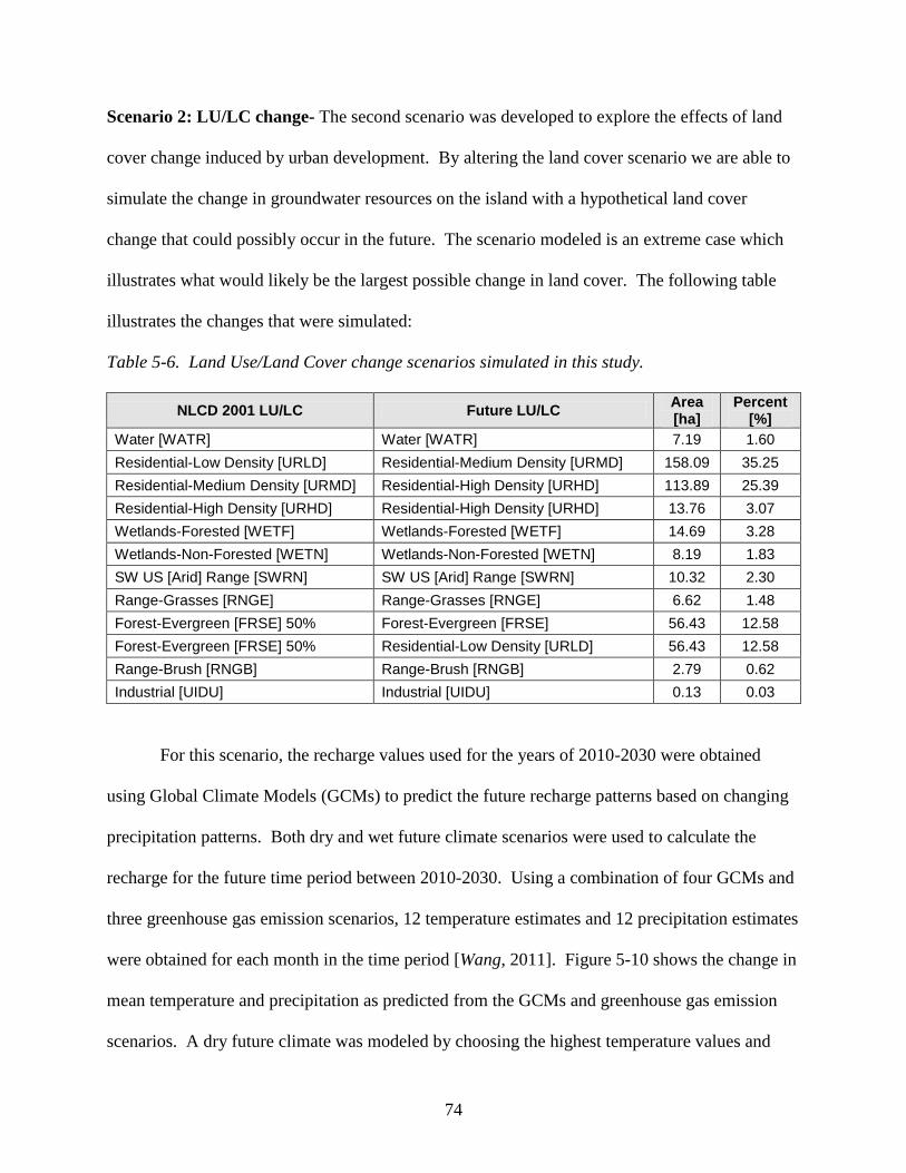
Table 5-6. Land Use/Land Cover change scenarios simulated in this study ...............................73
Table 5-7. Volume of freshwater in aquifer after scenario simulation ........................................89
Page 7
vii
List of Figures
Figure 2-1. Cross-Sectional view of a circular oceanic island [Chesnaux, 2008] .........................5
Figure 2-2. Measurement of recharge spike [from USGS Groundwater Information, 2008] ........9
Figure 3-1. Map of well locations used in this study ..................................................................18
Figure 3-2. Example of a hydrograph from the Baldwin County, AL well ................................21
Figure 3-3. Bin averaged MRC for Baldwin County, AL ..........................................................25
Figure 3-4. Bin averaged MRC for Montgomery ........................................................................25
Figure 3-5. Comparison of recharge methods in Minnesota [Delin et al., 2006] .......................26
Figure 3-6. Comparison of recharge methods in Baldwin Co, AL .............................................27
Figure 3-7. Land Cover/Land Use sites for FL Site #3, Baldwin, Covington, and Montgomery,
AL ............................................................................................................................33
Figure 3-8. Recharge versus continuing abstractions for seven sites .........................................36
Figure 3-9. Cumulative infiltration vs. cumulative recharge for seven sites ..............................37
Figure 3-10. Cumulative infiltration vs. cumulative recharge, Dec-April for five sites ...............38
Figure 4-1. Map of Mobile Bay and Dauphin Island ..................................................................40
Figure 4-2. Monthly temperatures for Dauphin Island in 2008 ..................................................41
Figure 4-3. Monthly precipitation for Dauphin Island from January 1995-December2005; data
from NCDC ..............................................................................................................42
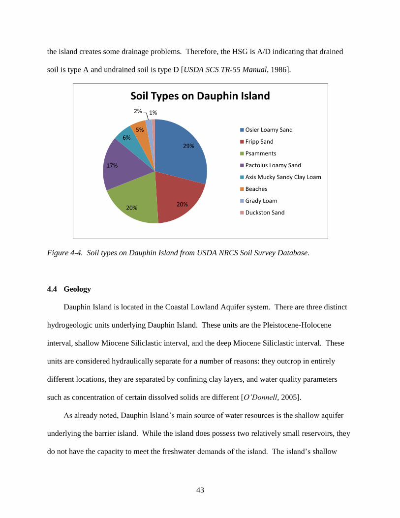
Figure 4-4. Soil types on Dauphin Island, USDA NRCS Soil Survey Database .......................43
Figure 4-5. Details of the layering of the aquifers beneath Dauphin Island [O’Donnell, 2005 ] 45
Figure 4-6. Land cover data from the Multi-Resolution Land Characteristics Consortium
[MRLC] ....................................................................................................................46
Figure 4-7. Well locations on Dauphin Island (well size is exaggerated). Blue color indicates
discharge towards the ocean ....................................................................................50
Page 8
viii
Figure 5-1. Comparison of precipitation and recharge for Dauphin Island, January 2000 - Dec
2004...............................................................................................................60
Figure 5-2. Locations of Alligator Lake and Oleander Pond on Dauphin Island .......................61
Figure 5-3. Steady state head distribution, April 2, 1985, from Kidd [1998] .............................68
Figure 5-4. Steady state head distribution, April 2, 1985, from model developed in this study 68
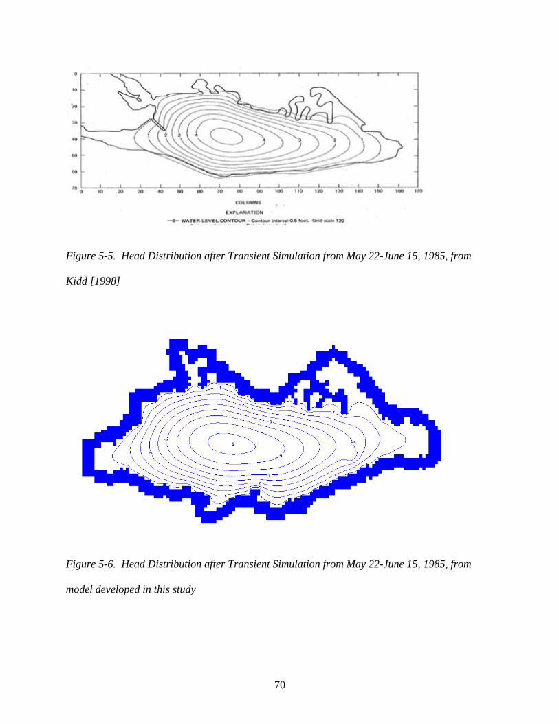
Figure 5-5. Head distribution after transient simulation from May 22-June 15, 1985, from Kidd
[1998] .......................................................................................................................69
Figure 5-6. Head distribution after transient simulation from May 22-June 15, 1985, from
model developed in this study ..................................................................................69
Figure 5-7. Head distribution after pumping simulation in 1988, from Kidd .............................70
Figure 5-8. Head distribution after pumping simulation in 1988, from model developed in this
study .........................................................................................................................70
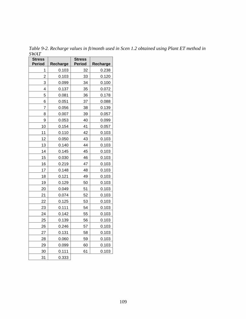
Figure 5-9. Recharge used for six scenarios as obtained from SWAT……………………….72
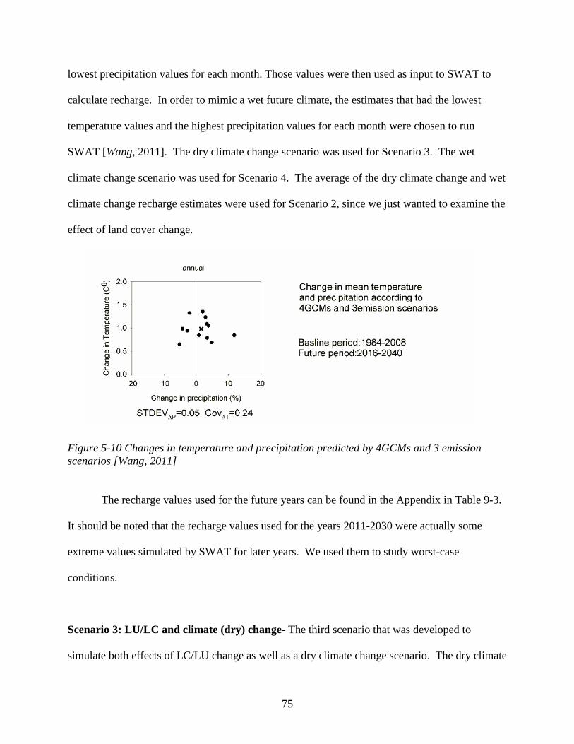
Figure 5-10. Changes in temperature and precipitation predicted by 4GCMs and 3 emission
scenarios [Wang, 2011] ...........................................................................................74
Figure 5-11. Dauphin Island population; data obtained from the United States Census Bureau .76
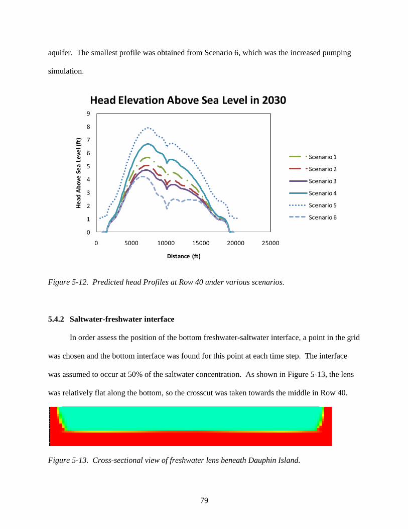
Figure 5-12. Predicted head profiles at Row 40 under various scenarios .....................................78
Figure 5-13. Cross-sectional view of freshwater lens beneath Dauphin Island ............................78
Figure 5-14. Location of crosscut taken at Row 40 ......................................................................79
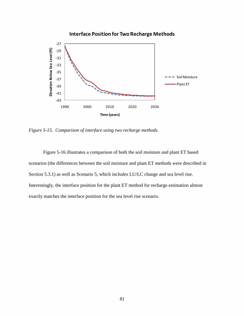
Figure 5-15. Comparison of bottom interface using two recharge methods .................................80
Figure 5-16. Comparison of bottom interface position using scenarios 1 and 5 ..........................81
Figure 5-17. Comparison of bottom interface position for all scenarios ......................................81
Figure 5-18. Saltwater-freshwater interface movement in Scenario 1.1.Red indicates saltwater,
aqua indicates freshwater .........................................................................................82
Figure 5-19. Saltwater-freshwater interface movement in Scenario 1.2. Red indicates saltwater,
aqua indicates freshwater .........................................................................................83
Figure 5-20. Saltwater-freshwater interface movement in Scenario 2. Red indicates saltwater,
aqua indicates freshwater .........................................................................................83
Page 9
ix
Figure 5-21. Saltwater-freshwater interface movement in Scenario 3. Red indicates saltwater,
aqua indicates freshwater .........................................................................................83
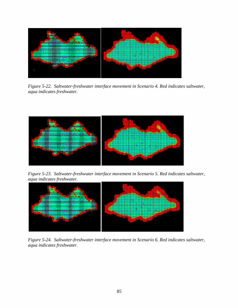
Figure 5-22. Saltwater-freshwater interface movement in Scenario 4. Red indicates saltwater,
aqua indicates freshwater .........................................................................................84
Figure 5-23. Saltwater-freshwater interface movement in Scenario 5. Red indicates saltwater,
aqua indicates freshwater ..........................................................................................84
Figure 5-24. Saltwater-freshwater interface movement in Scenario 6. Red indicates saltwater,
aqua indicates freshwater .........................................................................................84
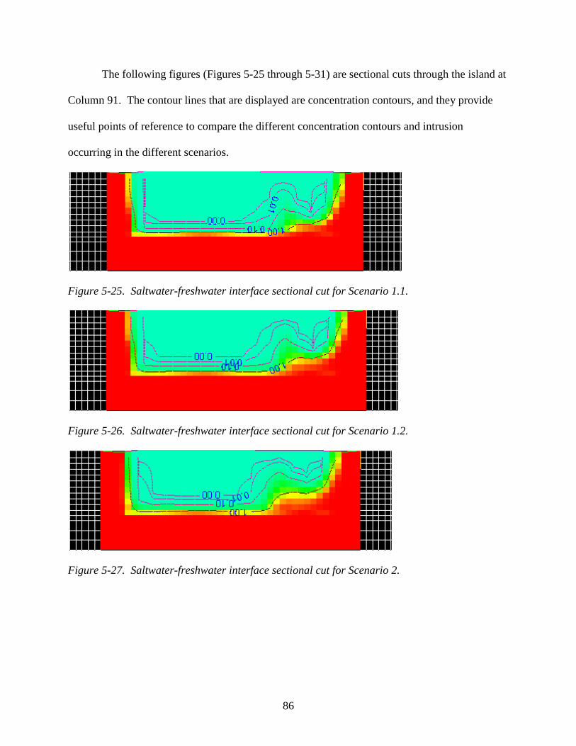
Figure 5-25. Saltwater-freshwater interface sectional cut for Scenario 1.1 ..................................85
Figure 5-26. Saltwater-freshwater interface sectional cut for Scenario 1.2 ..................................85
Figure 5-27. Saltwater-freshwater interface sectional cut for Scenario 2 .....................................85
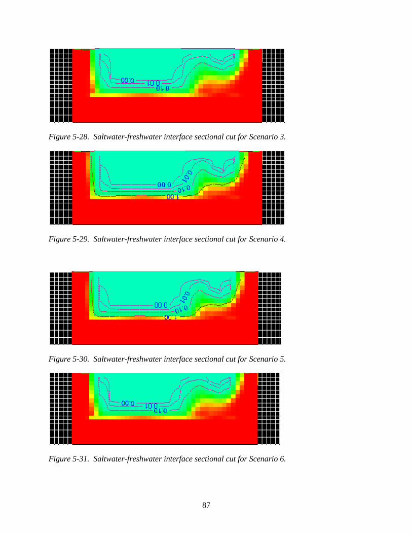
Figure 5-28. Saltwater-freshwater interface sectional cut for Scenario 3 .....................................86
Figure 5-29. Saltwater-freshwater interface sectional cut for Scenario 4 .....................................86
Figure 5-30. Saltwater-freshwater interface sectional cut for Scenario 5 .....................................86
Figure 5-31. Saltwater-freshwater interface sectional cut for Scenario 6 .....................................86
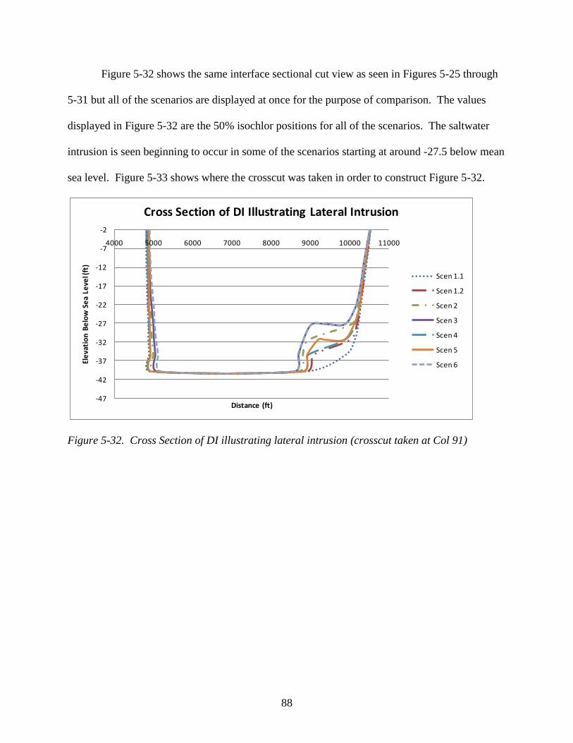
Figure 5-32. Cross Section of Dauphin Island illustrating lateral intrusion (crosscut taken at Col
91) ............................................................................................................................87
Figure 5-33. Location of crosscut taken at Column 91 .................................................................88
Figure 6-1. Concentration at monitoring well, detected concentration of 1.09 lbs/ft3 at 124
months ......................................................................................................................94
Figure 6-2. Isochlor at 124 mo, showing conc. of 1.09 lbs/ft3 reaching the monitoring well ....94
Figure 6-3. Concentration at monitoring well, detected concentration of 1.09 lbs/ft3 at 73 mo .95
Figure 6-4. Isochlor 73 months, showing concentration of 1.09 lbs/ft3reaching the monitoring
well ...........................................................................................................................95
Page 10
1
1. Introduction
Dauphin Island is a small barrier island located between the Mississippi Sound and the Gulf
of Mexico about 4 miles off the coast of Mobile County, Alabama [Chandler, 1983]. The
residents of Dauphin Island obtain their water from a shallow lens of freshwater located in the
island’s unconfined aquifer. According to the United States Census Bureau, the population of
Dauphin Island has been steadily increasing for the past 20 years. Due to the ever-growing
desire of Americans to live on the coast, it is reasonable to assume that this trend will continue.
Because of this, there is a need to understand the capacity, limitations, and characteristics of such
shallow coastal aquifers, and understand the impacts of changing climatic factors and hydrologic
parameters on these highly vulnerable water resource systems.
This research thesis consists of four sections. The first section investigates recharge issues in
the Southeast United States. Several recharge estimation methods were explored. The first
research question addressed in this section was which recharge estimation method gave
consistent results for our sites in the Southeast and should be used in the rest of the study? The
second research question was can a relationship be found between land cover type and amount of
water recharged into the aquifer?
The second section of this thesis provides background information about Dauphin Island. It
contains information on geology, soil, land use, and water problems of the island. It is intended
to introduce the reader to Dauphin Island hydrogeology and present the water issues faced by the
island.
The third section specifically focuses on the groundwater resources of Dauphin Island and
the effects of changing factors on the island’s water-table aquifer. The factors that were
examined in this section were the effects of land cover/land use change, climate change, and
Page 11
2
increasing population on the groundwater resources. The first research question considered is
whether changing the parameters based upon scenarios mimicking land-cover/land-use change,
climate change, and population change have a significant impact on the groundwater resources.
The second research question was if they did have a significant impact, which factors was the
aquifer most sensitive to.
The fourth section focused on assessing what percentage of Dauphin Island’s annual recharge
could be withdrawn from the wells without significantly impacting the aquifer. This study was
done because all of the scenarios modeled in the third study were hypothetical. Since it is
impossible to predict what the actual future recharge situation will be, it is important to know
what percentage of recharge can be pumped in order to make management decisions. The goal
was to estimate what percentage of the annual recharge on the island could be pumped without
saltwater contaminating any of the wells on the island.
Page 12
3
2. Literature survey
This chapter briefly introduces concepts and surveys relevant literature on several topics,
including groundwater aquifers and their importance in barrier islands, estimation techniques for
groundwater recharge, numerical modeling of groundwater, and other environmental factors that
affect groundwater resources.
2.1 Groundwater concepts for managing island aquifers
Increasing populations, increasing economic and industrial activities, and increasing
developments and urban sprawl around the world have significantly amplified demands on water
resources around the world. Depletion of surface water is becoming more evident in many areas,
putting an increased stress on groundwater sources. Additionally, some areas don’t have
naturally occurring surface water reservoirs or any considerable river systems. Because of this,
the demand for groundwater resources has become increasingly more substantial. Fortunately,
the amount of available freshwater in the form of groundwater is much higher than the amount
available as surface water, but usage of groundwater must be carefully managed [Fetter, 2001].
The existence of groundwater occurs when water is stored in the void spaces of soil,
fractured rock, or any other substance that makes up the underlying substrate. Groundwater can
occur in unconfined and confined aquifers. Unconfined aquifers have no confining layer
between the surface and the saturation zone. Confined groundwater is overlain by a confining
unit with a significantly lower hydraulic conductivity than that of the aquifer itself, and prevents
the flow of water through the confining strata [Fetter, 2001].
On small, barrier islands, the proportion of water used by humans coming from
groundwater is very high. Barrier islands are significantly smaller than continental landmasses.
Page 13
4
This means that there are no large watersheds feeding water to river systems. Additionally,
because of storms, tides, and sediment budget deficits, the morphology of barrier islands changes
almost constantly. Further, with sea level rise, there may be observable effects on the
morphology of the island [Morton, 2008]. Therefore, because of their relatively small size and
changing geomorphology, it is unlikely that there would be any well-established, major river
channels in these systems. Without any major river systems, reservoirs cannot be used to
provide a source of water for human consumption. Because of this, groundwater is extremely
important in barrier islands. Most of groundwater pumped from barrier islands comes from
island aquifer lens systems, a relatively shallow unconfined layer of water that is exploitable for
human use. Typically, these systems are precipitation derived freshwater lenses that overly
denser saltwater.
Chesnaux [2008] performed a detailed study of unconfined island aquifers. He specifically
developed analytical solutions for groundwater travel times in islands bounded by freshwater as
well as by seawater. Figure 2-4 illustrates the cross sectional view of an island aquifer system,
showing the lens of exploitable freshwater [Chesnaux, 2008].
Page 14
5
Figure 2-1. Cross-Sectional view of a circular oceanic island [Chesnaux 2008].
As shown in the figure, the sole source of input to the system is precipitation derived
recharge. Water is lost from the system via groundwater discharge occurring radially towards
the saline ocean. When the groundwater is pumped this is also a loss to the system [Chesnaux,
2008]. Withdrawals of water from these systems have serious consequences that must be
considered. If withdrawal rates from island aquifers are larger than recharge rates from
precipitation, saltwater intrusion will occur since the aquifer is in direct hydraulic contact with
the ocean.
Saltwater intrusion occurs because when water is pumped from island aquifers the inland
water level is reduced and the higher density salt water flows in due to the head gradient,
creating a saltwater wedge. As pumping continues, saltwater intrusion moves further inland and
eventually has the potential to contaminate the groundwater resources [Fetter, 2001]. In coastal
aquifers, intrusion can occur in a variety of modes. As already discussed, saltwater can intrude
Page 15
6
upward from deeper, saline zones, but intrusion can also occur laterally from the ocean as well as
downward from coastal waters [Barlow and Reichard, 2010].
The extent of the saltwater intrusion depends on factors such as rate of groundwater
withdrawls, distance between the pumping wells, geological properties of the aquifer, and the
hydraulic properties of the aquifer [Barlow and Reichard, 2010].
2.2 Groundwater recharge
Groundwater recharge is the process in which surface water reaches the water-table in the
aquifer’s phreatic zone [Martinez-Santos, 2010]. Groundwater recharge can occur in a variety of
ways. The two most common vehicles for recharge are deep seepage recharge occurring
between aquifer units and by infiltration recharge from precipitation.
As previously discussed, recharge is an integral part of the water budget for a shallow,
freshwater aquifer. Understanding and quantifying recharge is extremely important from an
aquifer planning and management standpoint so that sustainable abstraction levels can be
estimated for the aquifer. The rate and quantity of groundwater recharge directly affects the
quantity of freshwater resources contained in the aquifer, and the amount that can be safely
withdrawn. Shallow, precipitation driven aquifers are considerably sensitive to recharge rate.
Additionally, recharge estimates are important from a hydrogeological standpoint [Martinez-
Santos, 2010]. In order to accurately understand and model a specific aquifer system, there must
be a known estimate for recharge.
Additionally, being able to quantify recharge is also useful if saltwater intrusion occurs in
the aquifer. Under natural equilibrium conditions, high inland groundwater levels and flow of
fresh water to the sea impede inland movement of saltwater into aquifer systems, and the
Page 16
7
position of the boundary is a function of the amount of freshwater discharge [Fetter, 2001].
However, when aquifers are over exploited the salt water wedge advances into the aquifer and
saltwater intrusion occurs. The effect of recharge intensity and duration on saltwater intrusion
was studied by Mahesha and Nagaraja using a one-dimensional finite element model [1995].
They found that a relationship can be developed between interface motion of the saltwater wedge
and the intensity and duration of recharge.
There are at least three basic ways to obtain recharge at a certain location. The first, and
perhaps most obvious, is to measure it directly. This would include the use of expensive field
equipments. A potential drawback to direct measurement is the cost of equipment. Also, it is
known that this method is largely site specific [Sophocleous, 1991].
A second way to estimate recharge is using the hydrologic continuity equation as the
foundation. The equation is
sI Q
t
, where (2-1)
s
t
change in storage per time [L
3/t]; I inflow [L
3/t]; and Q outflow in [L
3/t].
This equation suggests that the change in the storage volume is quantified using the
difference between the inflow and outflow of a hydrologic system [Bedient and Huber, 1992].
This concept can also be applied to small basins by defining the terms that constitute the
inflow and the outflow. By doing this, the following water balance equation can be derived:
S P R G ET I , where (2-2)
S change in storage in a specified time period; P precipitation; R surface runoff; G
groundwater flow [recharge]; ET evapotranspiration, and I = interception [Bedient and Huber,
1992].
Page 17
8
The main problem with this method of recharge estimation is that while the input term,
precipitation, can be easily measured, many of the output terms are not easily measurable. Most
of the output terms either have to be measured with expensive equipment or estimated using
empirical relationships that are not always accurate for the given circumstance or site location.
For these reasons, this method is not always easy to apply or realistic.
The third method, which was the basis for the simpler method used later in this research,
is called the Water-Table Fluctuation (WTF) method. This method requires the input of
groundwater level data as well as an estimation of the specific yield of the aquifer. Specific
yield, Sy, is a property of rock or soil that indicates the ratio of the volume that the soil will yield
due to gravity drainage to the total soil volume [Fetter, 2001].
By measuring the fluctuations in groundwater level, the groundwater recharge can be
estimated. Each positive fluctuation in the groundwater level indicates recharge into the aquifer.
By measuring the change in groundwater level and multiplying the change by the specific yield
of the system, the value of groundwater recharge is found for that site. Mathematically, recharge
is calculated using the following equation:
( ) ( )j j yR t H t S , where (2-3)
( )jR t recharge from 0t to jt [L]; H the peak water level rise during the recharge period [L];
andyS Specific yield [dimensionless].
Page 18
9
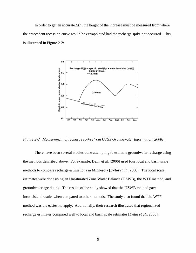
In order to get an accurate H , the height of the increase must be measured from where
the antecedent recession curve would be extrapolated had the recharge spike not occurred. This
is illustrated in Figure 2-2:
Figure 2-2. Measurement of recharge spike [from USGS Groundwater Information, 2008].
There have been several studies done attempting to estimate groundwater recharge using
the methods described above. For example, Delin et al. [2006] used four local and basin scale
methods to compare recharge estimations in Minnesota [Delin et al., 2006]. The local scale
estimates were done using an Unsaturated Zone Water Balance (UZWB), the WTF method, and
groundwater age dating. The results of the study showed that the UZWB method gave
inconsistent results when compared to other methods. The study also found that the WTF
method was the easiest to apply. Additionally, their research illustrated that regionalized
recharge estimates compared well to local and basin scale estimates [Delin et al., 2006].
Page 19
10
Crosbie et al. [2005] also used the WTF method, but combined it with a time series
approach to estimate recharge. Using the time series approach, long term water-table and
precipitation records were examined and effects due to evapotranspiration, atmospheric tides, the
Lisse effect, which occurs when air is trapped by infiltration, and varying specific yields values
were removed [Crosbie et al., 2005].
Recharge was estimated by Samper and Pisani [2009] using a combination of the soil
water balance and a groundwater flow model for Andújar alluvial aquifer in Spain. The soil
water balance alone gave too large of values for recharge estimates. The combined method
overcame common problems that are often encountered when recharge estimation is attempted
by soil water balance or groundwater flow models alone [Samper and Pisani, 2009].
Two recharge estimation methods were also combined by Sophocleous [1990] in an
attempt to quantify groundwater recharge in the Kansas Prairies. Sophocleous combined the soil
water balance and the WTF method to obtain his “hybrid water-fluctuation method.” For each
storm event, the recharge amount was calculated using the hydrologic budget. This amount was
divided by the measured water-table rise in the groundwater record for the corresponding event,
and the estimate of storativity was obtained. After this was done for several events, the average
storativity was found, and this value was applied to specific water-table rises to find groundwater
recharge values [Sophocleous, 1990].
In a study completed by Martínez-Santos and Andreu [2010] results from lumped and
distributed approaches to estimate recharge were compared for the Ventós Aquifer in Spain.
Lumped models assume the system can be expressed using a combination of transfer functions,
and the physics of recharge are rarely considered. Distributed models use detailed data records
to establish a relationship and provide spatial information. Both models obtained similar results,
Page 20
11
although the results from the lumped model agreed better with the available field data [Martínez-
Santos and Andreu, 2010].
Another problem that is often encountered in recharge estimation is difficulty in
measuring recharge for data poor areas. For example, some areas may not have groundwater
monitoring stations, so applying some of the previously discussed methods would be difficult.
Crosbie et al [2010] attempted to overcome such problems in their study of almost 200 sites in
Australia. They estimated recharge at 172 data rich sites in an attempt to obtain empirical
relationships that could relate recharge to national datasets and characteristics such as vegetation,
climate, and surface materials. This way the relationships could also be applied for data poor
areas. The study found that the relationships were most sensitive to vegetation and soil type
[Crosbie et al, 2010].
While hydrologic modeling was briefly mentioned earlier, a specific modeling tool to
estimate recharge that should be mentioned in depth, as it was used in this research project, is the
Soil Water Assessment Tool (SWAT). SWAT is a hydrologic continuous time model that was
developed to assess the effects of land management practices and climate on complex watersheds
[Arnold, 2005]. SWAT uses many input parameters and uses precipitation as the driver. One of
the outputs that can be obtained from the model is groundwater recharge for the watershed.
SWAT has been used in many instances to estimate groundwater recharge. For example,
Arnold et al. used it to estimate recharge in the upper Mississippi River Basin [Arnold et al.,
2000]. It was also used to quantify recharge in the Liverpool Plains of Australia by Sun and
Cornish [2005]. The specifics behind the SWAT procedures used in this research will be
discussed in later chapters.
Page 21
12
2.3 Density-dependent numerical modeling
As previously discussed, over exploitation of aquifers is currently stressing these systems
and causing distortion in the natural recharge-discharge equilibrium. Groundwater modeling has
become a powerful tool to visualize current groundwater flow conditions as well as predict
potential impact of future hypothetical scenarios. This aids in establishing long-term planning
practices for the aquifer. Groundwater flow models solve the general groundwater flow
equation, and are capable of providing visualization of either two or three dimensional flow in
aquifers. Many of these models are based on the popular MODFLOW groundwater model
[Harbaugh, 2000]. MODFLOW operates by using a finite difference solution scheme to solve
the three dimensional groundwater flow differential equation.
In order to simulate the interaction of saltwater and freshwater as well as the occurrence of
saltwater intrusion, a density-dependent groundwater flow model can be used [Lin et al., 2009].
SEAWAT was developed by combining MODFLOW and MT3DMS [Zheng, 1990] into one
program and making modifications to account for saltwater-freshwater density variations. By
doing this, a finite difference numerical model which is capable of solving the coupled flow and
solute transport equations was obtained [Guo and Langevin, 2002]. SEAWAT can use either an
implicit or explicit solution scheme. When solved implicitly, SEAWAT uses MODFLOW to
solve the flow field for each time step, and then MT3D to solve the concentration field. This
concentration is used to update the density field, which is used by MODFLOW as the relative
density difference term. This is repeated a number of times within the same time step until the
difference in density is smaller than the user-defined value [Rao et al., 2004]. When solved
explicitly, the flow and transport equations are solved alternately and repeated until the allotted
amount of stress periods are complete [Guo and Langevin, 2002].
Page 22
13
The SEAWAT modeling approach was validated by Goswami and Clement [2007] by
comparing laboratory data for both steady state and transient experiments to results obtained by
modeling done in SEAWAT [Goswami and Clement, 2007]. Previous to this, the benchmark for
validating saltwater intrusion models was the steady state Henry solution [Henry, 1964].
Many coastal aquifer studies have utilized SEAWAT to simulate the freshwater-saltwater
interface. For example, SEAWAT was used by Larabi et al. [2008] to model the groundwater
quantity and quality contained in the Rmel Coast aquifer in Morocco [Larabi et al., 2008].
Pravena and Aris [2010] used SEAWAT to model the aquifer underlying Manukan Island in
Malaysia. They modeled six scenarios representing possible human pressures and climate
change [Praveena and Aris, 2009]. SEAWAT was used by Lin et al. [2008] to model the degree
of saltwater intrusion in the Gulf coast aquifers of Alabama [Lin et al., 2008]. The study done by
Lin et al. included a 40 year predictive simulation run, which illustrated a large amount of
saltwater intrusion potential if groundwater pumping goes beyond the 1996 level. The paper
suggested a need for better groundwater development and management strategies for the Gulf
Coast, especially for the deep, confined aquifer systems.
An extensive modeling study using SEAWAT was done by Masterson [2004] to model the
complex groundwater system of Cape Cod, Massachusetts. The aquifer system at Cape Cod
consists of four distinct lenses. Increasing development and demand on the groundwater system
had raised serious concerns for the sustainability of the system. Using a complex groundwater
model, the current groundwater situation was simulated, as well as future groundwater levels
with predicted pumping rates [Masterson, 2004].
SEAWAT has also been used as a tool in a more unconventional manner to quantify aquifer
parameters. For example, Cecan et al. [2008] used it to analyze pumping test data in order to
Page 23
14
find horizontal hydraulic conductivity and vertical anisotropy in Cape Cod, Massachusetts. The
results of the study showed that classical methods such as the Hantush-Jacob method and
numerical models that do not account for density difference do not predict horizontal hydraulic
conductivity and vertical anisotropy values as accurately as SEAWAT [Cecan et al., 2008].
Rao et al. [2004] utilized SEAWAT in an unusual and interesting way. They used
SEAWAT to model the saltwater intrusion dynamics in a hypothetical coastal aquifer, but then
also explored if the SEAWAT model could be replaced by a trained artificial neural network.
An artificial neural network (ANN) is a computational tool that attempts to mimic the structure
and/or function of the biological neural network. Because of the computational burden that
corresponds with complex groundwater models, ANN was used to replace the model. In this
study, the ANN was improved by data training sets from repeated runs of SEAWAT. Once this
was done, the ANN was able to produce results very similar to the results obtained from
SEAWAT [Rao et al., 2004].
Other density dependent groundwater flow models have been used to model groundwater
flow in coastal aquifer systems. Joscon et al. [2001] used the SWIG2D to find the depth to the
saltwater interface in the Northern Guam Lens Aquifer [Joscon et al., 2001]. The region of the
Biscayne Aquifer underlying Hallandale, Florida was modeled by Anderson et al. [1988] using
the program SWICHA [Anderson et al., 1988]. Sherif and Singh [1999] used 2D-FED to model
the effects of climate change on two coastal aquifers, one in Egypt and one in India [Sherif and
Singh, 1999].
Page 24
15
2.4 Additional factors affecting groundwater resources in islands
While increased demand due to increasing population and pumping rates can cause large
stresses on an aquifer, there are other confounding factors that can affect the quality and quantity
of groundwater resources. Some of these factors are land cover/land use change and climate
change. Climate change includes scenarios such as changing precipitation patterns, increase in
hurricanes and other large storm events, and sea level rise.
Studies have been done that have illustrated the significant effects of land use on
groundwater recharge. By monitoring water level measurements from two monitoring wells for
122 days, Zhang and Schilling [2005] were able to observe the effects of land cover on the
water-table, evapotranspiration, soil moisture, and groundwater recharge. The two wells were on
either side of Walnut Creek, in Iowa. One of the wells was located in grassy field and the other
well was located in bare ground. The water level data showed significant variations in water
level between the two sites. Because of increased ET at the grass covered well, much less
groundwater recharge reached the water-table. They also found that soil moisture was also less
in the grass covered site due to ET [Zhang and Schilling, 2005].
Since there is often an obvious relationship between land use and recharge, scientists have
attempted to estimate recharge using land cover data. Cherkauer and Sajjad [2005] outlined a
method to estimate recharge which uses ground-surface information instead of long-term
groundwater monitoring data. They used the topography, hydrogeology, and land cover of the
site to estimate recharge. The method obtained a conservative approximation for recharge, but
recommended that the estimate should be refined with other methods [Cherkauer and Sajjad,
2005]. Similarly, Ranjan et al. [2005] estimated recharge based on land use and climatic factors.
They then used the estimated recharge amounts as inputs into a numerical groundwater model.
Page 25
16
Researchers have not only studied the effect of land use/land cover on groundwater
resources, but they have also studied the effect of land use/land cover change on aquifer systems.
Scanlon et al. [2005] completed a study on the Southwestern United States to test their
hypothesis that the land use/land cover (LU/LC) change of a natural rangeland into an
agricultural ecosystem will affect the groundwater recharge and chloride mass balance. By
examining three types of LU/LC they were able to detect significant differences in mean chloride
concentrations as well as mean matric potential. Information gained from this study and similar
studies suggest that groundwater resources can be somewhat managed through modification of
LU/LC [Scanlon et al., 2005].
Another factor that has the potential to significantly affect groundwater resources is climate
change. Since the mid-twentieth century carbon dioxide levels in the atmosphere have been
steadily rising. If this phenomenon continues, many researchers believe that the global and local
climate characteristics will be significantly altered [Ranjan et al., 2006]. This trend has been
termed climate change, and would likely have large effects on the hydrologic cycle around the
world. Increased atmospheric carbon dioxide levels would lead to an increased “greenhouse
effect,” in which solar radiation is trapped by the increased gases. This results in increased
temperatures, which in turn affects evapotranspiration, precipitation, and soil moisture.
While increased temperatures would likely lead to an overall global increase in
precipitation, it will lead to both increases and decreases on the local scale, depending on the
location and topography of the region [Ranjan et al., 2006]. There have been numerous studies
done which assess the impact of climate change and decreased precipitation on fresh
groundwater resources. Ranjan et al. [2006] used the high and low emissions scenarios from the
Hadley Centre climate model to predict the change in climate that should be input into their
Page 26
17
groundwater model. Among the five locations modeled, which were located around the globe,
all but one showed increasing losses of fresh groundwater resources.
Drought due to climate change could not only cause a decrease in groundwater recharge,
but also a decrease in water levels in surface reservoirs that would force more of a demand onto
groundwater. This situation was studied by Mollema et al. [2010] for Terceira Island in
Portugal. The water demands of the island are currently met by rain fed springs, but with
increased droughts they may need to begin to exploit the freshwater lens that underlies the island.
The study was devoted to understanding the size, characteristics, and limitations of the lens, so
that it could be exploited if necessary.
Another effect of climate change is sea-level rise. Sea level rise is caused by changes in
atmospheric pressure, expansion of ocean water, and the melting of ice sheets and glaciers
[Sherif and Singh, 1999]. The effects of sea level rise on saltwater intrusion have been studied
by Webb and Howard [2011], Loáiciga et al. [2011], and Chang et al. [2011]. Webb and
Howard [2011] found that the hydraulic properties of the aquifer played a large role in rate of
intrusion. Loáiciga et al [2011] found that groundwater pumping had a much larger effect on
saltwater intrusion than sea level rise. Chang et al. [2011] found that sea level rise does not have
a long-term impact on confined aquifers. While the sea level rise will initially cause saltwater
intrusion, a reversal effect will drive the wedge back out over time [Chang et al., 2011].
Page 27
18
3. Recharge and land cover estimation for the southeastern United States
This section discusses the process used to relate land cover type to groundwater recharge in
the Southeastern U.S. It discusses how land cover type and groundwater recharge values were
quantified as well as the methods used to find a relationship between the two factors.
3.1 Background
In order to obtain a relationship between groundwater recharge and land cover type, seven
sites were examined in the Southeast region. These sites were mostly located in coastal Alabama
and Florida, although two were located more inland than the others (Figure 3-1). They are all
located in un-consolidated and semi-consolidated shallow unconfined aquifers. The regional
aquifers that the well sites are located in are the Southeastern Coastal Plains aquifer, Coastal
Lowland aquifer, and the Floridian Sand and Gravel Surficial aquifer. The aquifers were all
unconfined with similar soil types, and the aquifer characteristics of the various regional aquifers
are similar. Therefore, after a small adjustment to specific yield values based on the site’s soil
characteristics, we can assume differences in recharge are due to land cover differences.
The sites labeled later in the research as FL1, FL2, and FL4 are in the
Gonzalez/Ensley/Pace area of Florida. Site FL3 is located in Pensacola, FL. The site labeled as
Covington was located in Covington County, AL, near Opp, AL. The site labeled Baldwin was
located in Baldwin County, AL, near Fairhope, AL. The site labeled Montgomery was located in
Montgomery, AL.
Page 28
19
Figure 3-1. Map of well locations used in this study.
3.2 Research objectives
The primary research objective of this section was to determine whether a relationship
could be derived between the groundwater recharge values and the land cover characteristics for
the seven sites in the Southeast. A significant relationship between the two factors would
indicate that land cover and land use is an important aspect in relation to groundwater resources
and the management of these resources. In an effort to obtain this relationship between
groundwater recharge and land cover characteristics, both continuing abstractions, which is the
amount of water taken into the soil once ponding begins, and infiltration were examined for the
seven sites.
This effort is valuable because whether or not a relationship can be derived between
groundwater recharge and LU/LC for the particular sites chosen is an interesting issue that is
worth investigating. If a relationship is found, the same concepts and methods could be later
Page 29
20
applied to find recharge in areas where there is no groundwater elevation data, but there is land
cover data. Specifically, the same methodology could be applied for Dauphin Island. As already
discussed, groundwater recharge is an important input for groundwater modeling. Dauphin
Island does not have publically available groundwater data from non-pumping wells, therefore; a
relationship between land cover and recharge would enable us to use the island’s land cover data
to calculate recharge.
Research methodology for this chapter is divided into three distinct parts. The first step
was estimating groundwater recharge for the seven sites. This was done using daily groundwater
level data from seven USGS groundwater monitoring wells. The recharge was calculated for a
year-long time period and summed to obtain an annual cumulative recharge value. A year-long
time period was used to eliminate the effects of differences in recharge rates due to seasonal
factors, such as changing evapotranspiration patterns in different seasons. The second section
describes how the Curve Number (CN) was used to relate recharge to land-cover and the third
part describes how the CN was calculated for each site.
3.3 Recharge estimation
This section discusses the methods examined for recharge estimation at the seven sites.
The results from the various methods are shown for a few of the sites in order to illustrate the
methods and then one method was selected as the best method for this study.
3.3.1 Methods and input data
The Water-Table Fluctuation (WTF) method, which was previously discussed, was the
method used to estimate cumulative recharge for the year-long time periods for each site. Since
the WTF method requires the peak water table rise during the recharge period, or H , as input to
calculate recharge, multiple methods were used and compared to generate H values.
Page 30
21
Perhaps the simplest method to measure groundwater recharge is the graphical method.
Using a hydrograph for a given site, which has groundwater elevation vs. time, the graphical
method can be completed manually. An example hydrograph for Baldwin County, AL is shown
in Figure 3-2. For each hydrograph spike, the height of the increase was measured from the
location the antecedent recession curve would be extrapolated had the spike not occurred. Prior
to extrapolating the curves, it is useful to examine the entire data set in order to get an estimate
for recession rates [USGS, 2008]. The measured heights were multiplied by the specific yield
values for each site. The recharge amounts were found, and Table 3-1 lists the values used for
specific yield in these calculations. The specific yield values were obtained by examining the
soil type at each of the seven sites. By summing the spikes for the year-long time period, the
cumulative recharge was found. The graphical method is prone to subjectivity when performed
manually as each person would likely draw the recession curve differently.
Figure 3-2. Example of a hydrograph from the Baldwin County, AL well.
Page 31
22
The second method of recharge estimation that was used was the Master Recession Curve
(MRC) approach to the WTF method. Developing a MRC is a similar idea to the graphical
method, but instead of manually extrapolating the hydrograph recession beneath each positive
fluctuation a MRC is developed to calculate the antecedent recession curve. A MRC is a water-
table recession hydrograph that is unique to the evaluated site. For a specific site it represents
the average behavior of a declining water-table [Heppner and Nimmo, 2005]. A MRC can be
developed using MATLAB [Heppner and Nimmo, 2005] or in Excel.
For this project, Excel was used to find the MRC for the various sites and the general
method is described in Heppner and Nimmo [2005]. In this method time and water level data for
the desired site is required. This data is used to calculate the water-table fluctuation rate for each
time step. The water table fluctuation rate is the change in water table elevation divided by the
change in time for each time step. The water-table fluctuation rate is plotted on the y-axis
against the water-table elevation on the x-axis.
This method assumes that at a certain water-table elevation, there will be a characteristic
water-table decline rate. Due to this, we would expect a linear relationship when the data is
plotted. However, due to various factors, this may not always be the case. The type of MRC
that can be created is selected based on the trend in the plotted data. In addition to a linear
method, power and bin averaged may also be used [Heppner and Nimmo, 2005]. The bin
averaged method was used for this research, so it will be discussed more in depth.
The bin-averaged method is best suited for large data sets that may have an irregular
pattern when initially plotted [Heppner and Nimmo, 2005]. After inspecting the range of
elevation values from the lowest to highest observed water-table elevations, the user decides on
an appropriate number of bins, which are ranges of elevation, based on the elevation range. The
Page 32
23
total range is then divided into equally spaced bins of elevation range. As the elevation levels
are placed into the appropriate elevation bins, the corresponding decline rates are placed in the
bins [Heppner and Nimmo, 2005]. Each elevation and decline rate bin is averaged and plotted.
Once these values are plotted the relationship usually appears more linear and a trend line
equation can be obtained that is specific for the particular site and time period.
The equation obtained represents the MRC. For example, a hypothetical MRC may be
represented by the equation y mx b . Given a dataset that contains time as well as
groundwater elevation values, the equation can then be used to find total recharge. For each time
step, the groundwater level in from the previous time step is used as the x-value, and the y-value
is the predicted groundwater level from the Master Recession Curve. By subtracting the
predicted value from the actual value, H is obtained. This H is subsequently multiplied by
the specific yield of the aquifer to obtain the recharge.
The third method used to obtain H and thus cumulative recharge, mimicked the RISE
program developed by Rutledge [2007]. This program calculates the daily rise in a given
observation well by calculating the amount of water level increase from the previous day. The
value for that day is set to zero if the difference is negative, but it is considered groundwater
recharge if the difference is positive [Delin et al., 2006]. Daily recharge values are evaluated
using this program and the positive recharge values are summed to obtain a cumulative annual
rise in the aquifer (cumulative H ). This estimate was multiplied by the specific yield of the
subsurface material to obtain the cumulative annual recharge.
Specific yield values were varied based on the soil material of the site. Soil data was
obtained from the SSURGO database and imported into ArcMap program as a shapefile. The
well locations were marked on their latitude and longitude. Using the soil types of the region, a
Page 33
24
specific yield value was assigned to each site. The values that were used for specific yield were
based on values from Fetter [2001], Nachabe [2002], and estimations based on these ranges and
soil types. The specific yield was used to multiply H to obtain the daily and cumulative annual
recharge for each site. Table 3-1 shows the values specific yield values of each site:
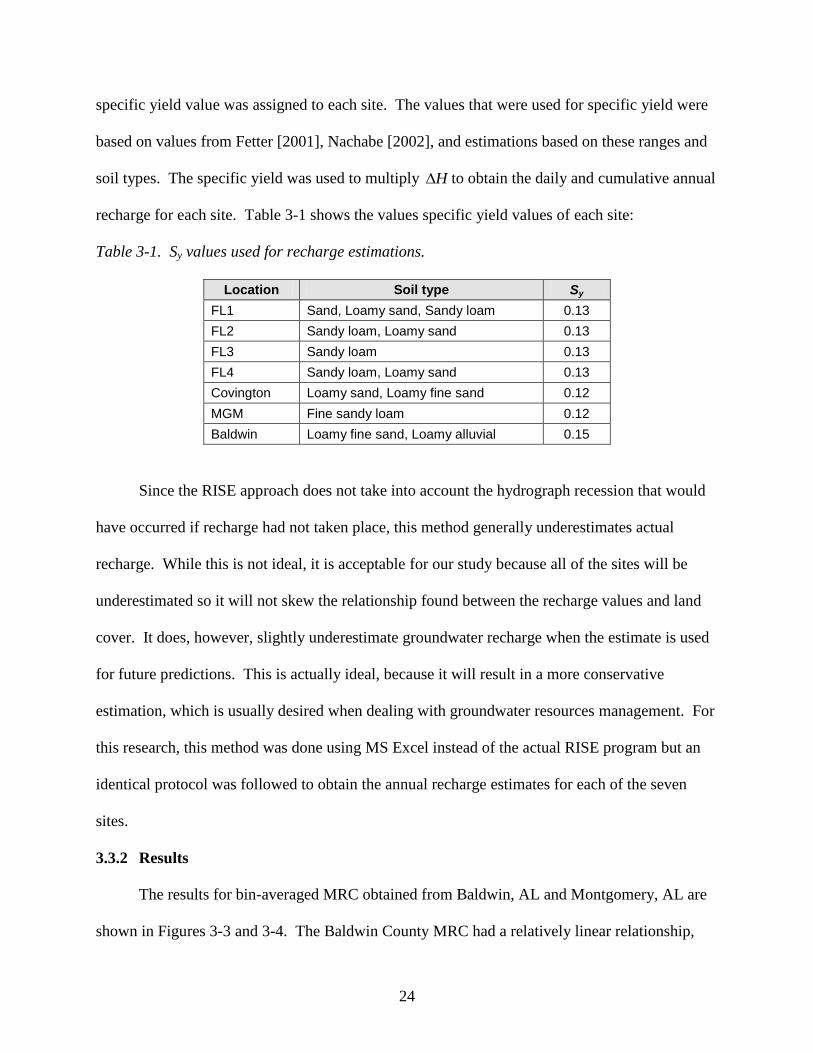
Table 3-1. Sy values used for recharge estimations.
Location Soil type Sy
FL1 Sand, Loamy sand, Sandy loam 0.13
FL2 Sandy loam, Loamy sand 0.13
FL3 Sandy loam 0.13
FL4 Sandy loam, Loamy sand 0.13
Covington Loamy sand, Loamy fine sand 0.12
MGM Fine sandy loam 0.12
Baldwin Loamy fine sand, Loamy alluvial 0.15
Since the RISE approach does not take into account the hydrograph recession that would
have occurred if recharge had not taken place, this method generally underestimates actual
recharge. While this is not ideal, it is acceptable for our study because all of the sites will be
underestimated so it will not skew the relationship found between the recharge values and land
cover. It does, however, slightly underestimate groundwater recharge when the estimate is used
for future predictions. This is actually ideal, because it will result in a more conservative
estimation, which is usually desired when dealing with groundwater resources management. For
this research, this method was done using MS Excel instead of the actual RISE program but an
identical protocol was followed to obtain the annual recharge estimates for each of the seven
sites.
3.3.2 Results
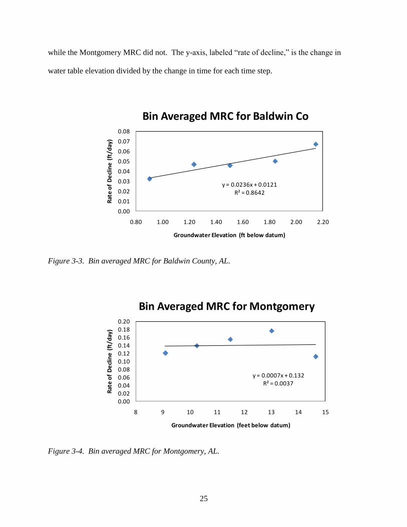
The results for bin-averaged MRC obtained from Baldwin, AL and Montgomery, AL are
shown in Figures 3-3 and 3-4. The Baldwin County MRC had a relatively linear relationship,
Page 34
25
while the Montgomery MRC did not. The y-axis, labeled “rate of decline,” is the change in
water table elevation divided by the change in time for each time step.
Figure 3-3. Bin averaged MRC for Baldwin County, AL.
Figure 3-4. Bin averaged MRC for Montgomery, AL.
y = 0.0236x + 0.0121R² = 0.8642
0.00
0.01
0.02
0.03
0.04
0.05
0.06
0.07
0.08
0.80 1.00 1.20 1.40 1.60 1.80 2.00 2.20
Rat
e o
f D
ecl
ine
(ft
/day
)
Groundwater Elevation (ft below datum)
Bin Averaged MRC for Baldwin Co
y = 0.0007x + 0.132R² = 0.0037
0.000.020.040.060.080.100.120.140.160.180.20
8 9 10 11 12 13 14 15
Rat
e o
f D
ecl
ine
(ft
/day
)
Groundwater Elevation (feet below datum)
Bin Averaged MRC for Montgomery
Page 35
26
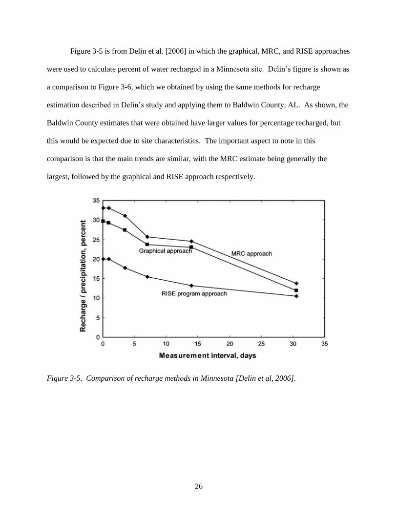
Figure 3-5 is from Delin et al. [2006] in which the graphical, MRC, and RISE approaches
were used to calculate percent of water recharged in a Minnesota site. Delin’s figure is shown as
a comparison to Figure 3-6, which we obtained by using the same methods for recharge
estimation described in Delin’s study and applying them to Baldwin County, AL. As shown, the
Baldwin County estimates that were obtained have larger values for percentage recharged, but
this would be expected due to site characteristics. The important aspect to note in this
comparison is that the main trends are similar, with the MRC estimate being generally the
largest, followed by the graphical and RISE approach respectively.
Figure 3-5. Comparison of recharge methods in Minnesota [Delin et al, 2006].
Page 36
27
Figure 3-6. Comparison of recharge methods in Baldwin Co, AL.
Table 3-2 summarizes the values obtained for cumulative recharge at each site using the
RISE method.
Table 3-2. Recharge values using the RISE method.
Site Location Dates Evaluated Rise Recharge
Estimate [ft] Precip
[ft]
FL1 7/1/1981-6/30/1982 1.75 3.79
FL2 10/1/1983-9/30/1984 3.60 4.94
FL3 9/7/1983-9/6/1984 1.21 5.36
FL4 1/15/1980-1/14/1981 2.10 4.05
Covington Co 5/1/2007-4/30/2008 3.53 4.56
Montgomery Co 1/27/1990-1/26/1991 1.81 4.13
Baldwin Co 11/1/2007-10/31/2008 1.63 6.28
3.3.3 Observations
The graphical method was deemed inefficient and subjective because different results are
obtained by different users of the method, hence the results of this method will not be used
further in this study. For some of the sites evaluated in this study, the line of best fit generated
using the MRC method had a high R2 value (Figure 3-2) and the relationship would have been
0.00
0.10
0.20
0.30
0.40
0.50
0.60
0.70
0.80
0.90
60 110 160 210 260 310 360 410 460
Re
char
ge/p
reci
pit
atio
n,
pe
rce
nt
Measurement interval, days
Baldwin County Recharge
MRC Approach
RISE program approach
Graphical approach
Page 37
28
acceptable for use in estimating recharge. For other sites, however, the relationship had a
relatively low R2 value (Figure 3-3) and the relationship was deemed insignificant and not
acceptable for use in this study. This is most likely due to other factors causing a difference in
recharge rate, such as antecedent moisture conditions, the Lisse Effect, and heterogeneities in the
subsurface material. Due to this, the RISE method of recharge estimation was employed in order
to quantify the amount of annual recharge at the seven sites, and the RISE estimates were used in
the following sections of this chapter.
3.4 Quantify LU/LC effects on Recharge
This section discusses the method used in an attempt to relate LU/LC to the amount of
water recharged into the aquifer at each of the seven sites.
3.4.1 Study methodology and input data
The Soil Conservation Service Curve-Number (SCS-CN) method was developed by the
United States Department of Agriculture-Soil Conservation Service (USDA-SCS) in the 1950’s.
The SCS-CN method can be used to predict flood-flow volumes for ungauged watersheds for
runoff generating rainfall events [Lyon et al., 2004]. Accumulated rainfall (P) and accumulated
runoff (Q) are important variables in the SCS-CN method. Therefore, the general form of the
SCS-CN equation is as follows:
SIP
IPQ
a
a
2)(
(3-1)
where Q is runoff [in], P is the event precipitation [in]; aI is the initial abstractions [in]; and S is
the potential maximum retention after runoff begins [in]. This equation is only valid if P>Ia. If
this precipitation is not greater than the initial abstractions, Q=0. The CN is used to calculate
both S and Ia [Michel et al., 2005]. The equations for both of these variables will be outlined
Page 38
29
below. The CN is a function of LU/LC, Hydrologic Soil Group (HSG), and the Antecedent
Moisture Condition (AMC) of the soil.
Once the appropriate adjusted CN was found for each day in the precipitation record, it
was used along with daily precipitation records for the area to calculate the continuing
abstractions, Fa, for events that qualify. As will be illustrated in the following calculations, Fa is
calculated using both CN and precipitation, so it takes into account land cover type as well as
precipitation events. This makes it a sensible value to use in developing a relationship between
recharge and LU/LC type.
The value of initial abstractions, or aI , is calculated to determine which events qualify as
large enough to generate continuing abstractions. aI includes interception by vegetation and
water that ponds on the surface [Lecture Notes, Kalin, 2010]. In order to obtain aI , the adjusted
CN value was used to first calculate S using equation 3-2. The method and calculations for
obtaining the CN will be described in Section 3.5:
101000
CN
S (3-2)
where S is the potential maximum retention after runoff begins [in]; and CN is the curve number
[dimensionless].
With S , the value of the initial abstraction of water during a rainfall event could be
calculated using the following equation:
SIa *2.0 (3-3)
The calculated aI values were used to determine which rainfall events were large enough
to generate continuing abstractions. As already stated, for each rainfall event, the total amount of
Page 39
30
precipitation must be larger than or equal to S*2.0 in order for the event to generate continuing
abstractions. The values of aI and S were subsequently used to calculate the value of runoff, or
,Q using equation 3-1 that was presented above.
Using the obtained values the continuing abstractions can be calculated through equation
3-4:
QIPF aa . (3-4)
The sum of the aF values for the annual period for each site were plotted against the
recharge values for the respective sites on the same scatter plot (Figure 3-7) to seek a relationship
between recharge and aF . If a relationship is found between recharge and aF , this relationship
could be related back to land cover type as described above. With a relationship between the two
factors, recharge could be calculated using the average CN of a particular site.
As an alternative, a relationship between infiltrating depth and recharge was also sought
to see if a relationship between LU/LC and recharge could be developed. First interception
depth was calculated using the following equation [Bras, 1990] :
* nI a b P (3-5)
where I is interception [in]; , ,a b and n are empirical values that vary with vegetation type; and
P is the amount of precipitation [in].
Interception is the amount of rainfall that is intercepted by vegetation before it is able to
reach the ground [Fetter, 2001]. Once interception was calculated, infiltration was estimated by
subtracting Q and interception from total precipitation for each rain event.
The values that were calculated for each site were plotted against the recharge values for the
respective sites on the same scatter plot to find a relationship between recharge and land cover
Page 40
31
(Figure 3-8). Additionally, the data points from a few of the sites seemed less reliable and these
locations were removed from the analysis. The relationship was observed for the time period of
December to April (Figure 3-9). This time period was examined because it can be assumed that
the least evapotranspiration would be occurring during this time period, causing the infiltration
values to be greater. The sites that were not included in this last plot were the Montgomery, AL
site and the Baldwin County, AL site since Montgomery is more inland than the others and the
Baldwin County site could have been tidally influenced as it is very close to the coast.
3.5 Land cover analysis and curve number calculations
This section details the method used to utilize land cover/land use data in order to calculate
the curve number for a given land area. Average curve numbers were obtained for each of the
seven study sites. As previously explained, the SCS-CN method has been widely used for years
as a tool to calculate the volume of surface runoff for rain events, reflecting factors such as
LU/LC effects [Mishra and Singh, 2011].
Page 41
32
3.5.1 Study methodology and input data
After an annual recharge estimate was found using the RISE estimation method for the
seven sites, the next step was to quantify land cover type for each site. Land cover data was
obtained from the National Land Cover Database (NLCD). Using the latitude and longitude of
the well locations, data was downloaded for the region surrounding the well. Landcover data
downloaded from NLCD was imported into ArcMap and cropped. An ellipsoid shaped boundary
with 100 meters from the well to the side of the ellipse and 200 meters to the top of the ellipse
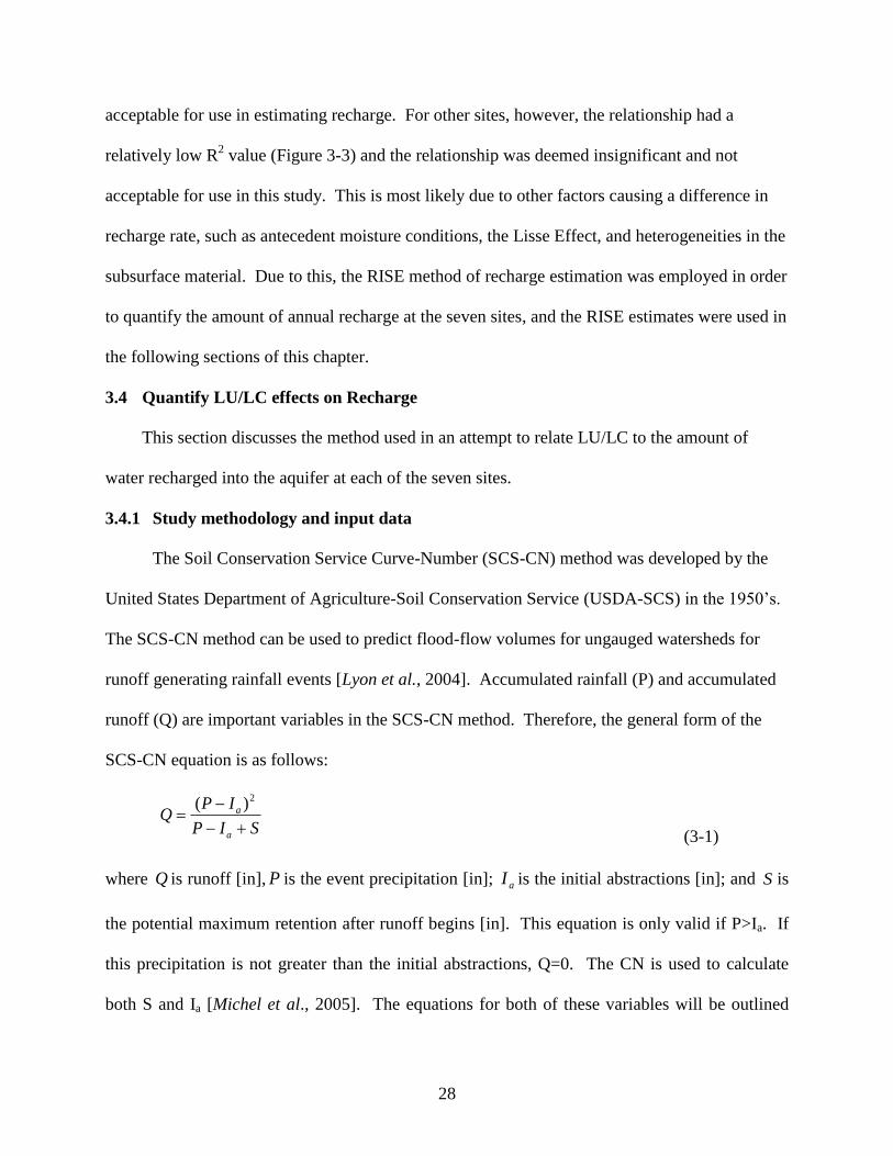
was applied around the well. The orientation of the ellipse was decided by the direction of flow
on the surface, as it was assumed that the shallow subsurface flow approximately mimics the
direction of the surface flow.
The land cover map was cropped and a measured grid was applied with grid cells of 20 m
x 20 m (Figure 3-6). Each grid cell was assigned a land cover type that occupied the majority of
each cell.
Page 42
33
Figure 3-7. Land Cover/Land Use sites for FL Site #3, Baldwin, Covington, and Montgomery,
AL.
A curve number was assigned to each grid based on land cover type. The curve number,
CN, is an empirical value that is used in predicting runoff or infiltration and is a function of
hydrologic soil group, land cover type, land cover treatment, and hydrologic condition such as
antecedent moisture condition [USDA SCS TR-55 Manual, 1986].
The curve number for each land cover type depends on the hydrologic soil group of the
soil in area. The hydrologic soil group indicates the soil’s tendency for infiltration or runoff.
The hydrologic soil group for each soil type was obtained from the NRCS Web Soil Survey
Page 43
34
(websoilsurvey.nrcs.usda.gov/). Using the hydrologic soil group, a CN value was assigned for
each grid.
Next, the distance between the monitoring well and the center of each cell was calculated.
The inverse of the distances were used to weight the CN of each cell, and an average CN was
obtained for each well site using the weighted CN values.
In order to accurately use the average CN, the antecedent moisture condition (AMC) had
to be taken into account. The average CN that was calculated in the previous step is for normal
conditions (CN2) and a CN1 can be found for a dry AMC, while conversely a CN3 is used for a
wet AMC. Table 2-2 outlines the antecedent moisture values that dictate which CN value should
be used [Chow et al., 2005]:
Table 3-3. Values used to determine AMC.
AMC Total 5-day antecedent precipitation [in]
Dormant Season Growing Season
I < 0.5 < 1.4
II 0.5 to 1.1 1.4 to 2.1
III > 1.1 > 2.1
Daily precipitation data was obtained from the National Climatic Data Center (NCDC)
for the same year-long time period for each site in which the recharge measurements were made.
Table 3-4 lists the appropriate weather station ID used for each of the wells, and the approximate
distance from the weather station to the groundwater well.
Page 44
35
Table 3-4. Approximate distance from well to weather station
Site Name Well ID Weather Station Distance: well to station
[mi]
FL 1 USGS303610087165001 Pensacola Reg Airport 13
FL 2 USGS303558087155501 Pensacola Reg Airport 13
FL 3 USGS30283008711390 Pensacola Reg Airport 1.25
FL 4 UGSG303614087190901 Pensacola Reg Airport 13
Covington Co USGS311319086153601 Andalusia, AL 18
MGM Co USGS322047086214301 MGM Airport 6
Baldwin Co USGS302416087505501 Fairhope, AL 12
Using this data, the AMC for each day in the record was calculated by summing the five
previous day’s precipitation amounts. Based on this sum for each day, the CN number was
calculated accordingly using equations 3-6 and 3-7 for wet and dry conditions respectively
[Chow et al., 2005]:
)(058.010
2.4
2
21 dry
CN
CNCN
(3-6)
23
2
23( ).
10 0.13
CNCN wet
CN
(3-7)
3.5.2 Results
The Table 3-5 shows the average calculated values of CN. As illustrated, the values that
were calculated vary widely from site to site, depending on the land cover type. For example,
the site labeled FL3, which has a very large CN is located in the Pensacola Regional Airport. In
contrast, the site labeled FL1 is located in an area that is heavily forested.
Page 45
36
Table 3-5. Calculated average CN values.
Site Location Calculated Avg CN
FL1 50
FL2 59
FL3 93
FL4 76
Covington Co 84
Montgomery Co 77
Baldwin Co 78
Figure 3-8 is the scatter plot of the seven site’s cumulative recharge values plotted against
each site’s cumulative continuing abstraction values.
Figure 3-8. Recharge versus continuing abstractions.
y = -0.3265x + 30.929R² = 0.0097
05
101520253035404550
0 5 10 15 20
Re
char
ge (
in)
Continuing Abstractions, Fa (in)
Continuing Abstractions vs. Recharge
Page 46
37
Figure 3-9 shows the scatter plot of cumulative recharge and cumulative infiltration for
each site.
Figure 3-9. Cumulative Infiltration vs. Cumulative recharge
Figure 3-10 shows the scatter plot of cumulative recharge plotted against cumulative
infiltration at five of the sites for December to April. As stated earlier, these calculations were
done using only data from December to April, as the least evapotranspiration occurs during these
months, and the sites of Baldwin County, AL and Montgomery, AL were not used in an effort to
obtain a better relationship. As stated previously, these sites were left out since Montgomery is
more inland than the other sites and the Baldwin County site could have been tidally influenced.
y = 0.997x - 8.4164R² = 0.213
05
101520253035404550
0 10 20 30 40 50
Re
char
ge (
in)
Infiltration (in)
Infiltration vs. Recharge
Page 47
38
Figure 3-10 Cumulative Infiltration vs. Cumulative Recharge for December-April
3.5.3 Discussions
As illustrated in the figures, no significant linear relationship was found between aF and
recharge or the infiltration values and recharge. The seasonal investigation of infiltration and
recharge did not yield any significant results either. This is likely due to a number of
confounding factors. Some factors that may have contributed to an unclear relationship between
land use and recharge could have been due to some of the water-tables being deeper than others,
unpredictable heterogeneities in the soil profiles causing flow impediment or changing specific
yield values, or the Lisse effect, which occurs when air is trapped by recharging water causing
the water level to be at a higher level than it would appear if only the recharged water height was
taken into account. Many of the recharge values calculated using the RISE method seemed
larger than would be expected. For example, there was an instance that the recharge value
exceeded the infiltration value for the same site, which is physically impossible. This would
suggest that there were factors influencing the recharge estimate. Also, it is possible that the area
y = 1.1134x - 0.4583R² = 0.326
0
5
10
15
20
25
0 5 10 15 20
Re
char
ge (
in)
Infiltration (in)
Infiltration vs. Recharge: Dec-April
Page 48
39
of land taken into account for the CN calculations was too large, although the weighting scheme
should have taken this into account.
Due to the fact that there was no clear relationship found between land cover and recharge in
this study, this method was not used to calculate average annual recharge on Dauphin Island with
land cover data. Instead, recharge estimates were obtained by directly applying the Soil Water
Assessment Tool (SWAT) which will be explained in further detail in Chapter 5.
Page 49
40
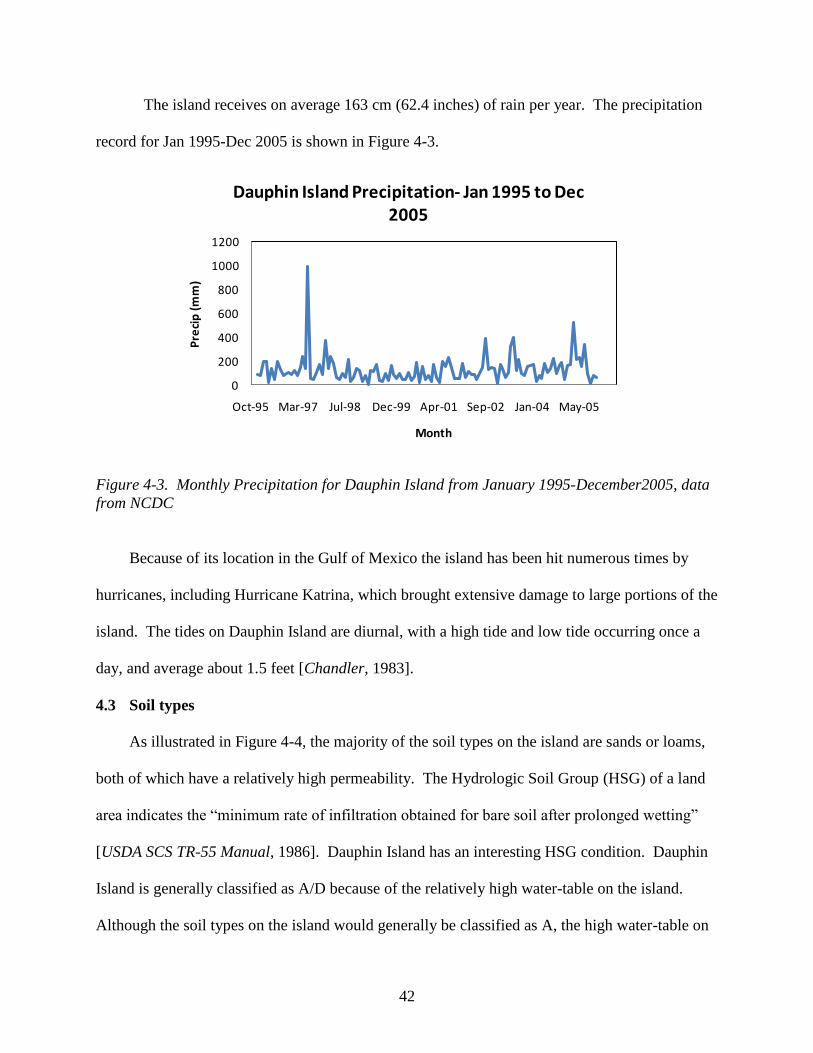
4. Geography and ground water issues of Dauphin Island
This chapter provides necessary background information on Dauphin Island and also
summarizes the island’s current water issues.
4.1 Location, size, and morphology
Dauphin Island is a small barrier island located between the Mississippi Sound and the Gulf
of Mexico about 4 miles off the coast of Mobile County, Alabama (Figure 4-1). The island is
shaped like an oval on the east end, with a thin strip of land coming off the oval to make up the
west end (Figure 4-1). The east end oval is about 1.5 miles wide at its widest and 3 miles long.
The thin strip of land that makes up the west end is about 12 miles long and 0.5 miles wide. In
total, Dauphin Island is about 6.3 square miles in size. Elevation on the island mostly varies
between 5 to 15 feet but can reach up to 40 feet at the locations of the island’s sand dunes
[Chandler, 1983].
Figure 4-1. Map of Mobile Bay and Dauphin Island.
Page 50
41
Since Dauphin Island is a barrier island its morphology is constantly changing as a result of
coastal winds, tides, and currents. The shoreline of the island has greatly varied throughout
history, mostly due to longshore drift and hurricanes. Longshore drift, which is the process of
sediment transport along the coast, is likely responsible for the formation of the long,thin sandy-
spit extension on the west end of the island. Vegetation on this island is important as it prevents
erosion and promotes accretion in some areas. Additionally, the marsh areas are nutrient
processing sites [Chandler, 1983].
4.2 Climate and tides
The climate of Dauphin Island is significantly influenced by the Gulf of Mexico and is warm
to subtropical. Temperature variations on Dauphin Island in 2008 are shown in Figure 4-2.
Monthly average temperature variations are less than 20F from the annual mean [Chandler,
1983]. The annual average maximum temperature is 74.8 °F and the average minimum
temperature is 63.1 °F.
Figure 4-2. Monthly temperatures for Dauphin Island in 2008.
Page 51
42
The island receives on average 163 cm (62.4 inches) of rain per year. The precipitation
record for Jan 1995-Dec 2005 is shown in Figure 4-3.
Figure 4-3. Monthly Precipitation for Dauphin Island from January 1995-December2005, data
from NCDC
Because of its location in the Gulf of Mexico the island has been hit numerous times by
hurricanes, including Hurricane Katrina, which brought extensive damage to large portions of the
island. The tides on Dauphin Island are diurnal, with a high tide and low tide occurring once a
day, and average about 1.5 feet [Chandler, 1983].
4.3 Soil types
As illustrated in Figure 4-4, the majority of the soil types on the island are sands or loams,
both of which have a relatively high permeability. The Hydrologic Soil Group (HSG) of a land
area indicates the “minimum rate of infiltration obtained for bare soil after prolonged wetting”
[USDA SCS TR-55 Manual, 1986]. Dauphin Island has an interesting HSG condition. Dauphin
Island is generally classified as A/D because of the relatively high water-table on the island.
Although the soil types on the island would generally be classified as A, the high water-table on
0
200
400
600
800
1000
1200
Oct-95 Mar-97 Jul-98 Dec-99 Apr-01 Sep-02 Jan-04 May-05
Pre
cip
(m
m)
Month
Dauphin Island Precipitation- Jan 1995 to Dec 2005
Page 52
43
the island creates some drainage problems. Therefore, the HSG is A/D indicating that drained
soil is type A and undrained soil is type D [USDA SCS TR-55 Manual, 1986].
Figure 4-4. Soil types on Dauphin Island from USDA NRCS Soil Survey Database.
4.4 Geology
Dauphin Island is located in the Coastal Lowland Aquifer system. There are three distinct
hydrogeologic units underlying Dauphin Island. These units are the Pleistocene-Holocene
interval, shallow Miocene Siliclastic interval, and the deep Miocene Siliclastic interval. These
units are considered hydraulically separate for a number of reasons: they outcrop in entirely
different locations, they are separated by confining clay layers, and water quality parameters
such as concentration of certain dissolved solids are different [O’Donnell, 2005].
As already noted, Dauphin Island’s main source of water resources is the shallow aquifer
underlying the barrier island. While the island does possess two relatively small reservoirs, they
do not have the capacity to meet the freshwater demands of the island. The island’s shallow
29%
20% 20%
17%
6% 5%
2% 1%
Soil Types on Dauphin Island
Osier Loamy Sand
Fripp Sand
Psamments
Pactolus Loamy Sand
Axis Mucky Sandy Clay Loam
Beaches
Grady Loam
Duckston Sand
Page 53
44
aquifer consists of a thin layer of Holocene sand, which is underlain by a Pleistocene unit known
as the Gulfport Formation. The aquifer is approximately 28-42 feet thick with a thick layer of
marine clay at the base. The water in Dauphin Island’s aquifer is generally low in chloride
content except near the island’s coast. Recharge to the aquifer occurs through rainfall.
Freshwater is lost from the aquifer due to seepage to surface water, evapotranspiration and
pumping [Kidd and Moody, 1987].
As discussed, the top unit visible from the ground level is the Water-Table Aquifer. This
aquifer extends about 42 feet below ground level and is composed of fine to coarse grain sand
[O’Donnell, 2005]. A layer of clay underlies this aquifer and separates it from the Shallow Sand
Aquifer, which occurs at about 70 feet below ground level and is composed of very fine to very
coarse grain quartzose sand [O’Donnell, 2005]. The top surficial aquifer is hydraulically
separate from the other aquifers located below it.
There are three layers of the Shallow Sand Aquifer, each of which has a clay layer
underneath. Another clay layer underlies the Shallow Sand Aquifer. Beneath this clay layer is
the Deep Sand Aquifer, which begins at about 441 feet below the surface.
The Water-Table Aquifer and the Shallow Sand Aquifer are the only units deemed potential
sources of freshwater without rigorous treatment. The water pumped from the Deep Sand
Aquifer has a chloride concentration too high to be used for human consumption [O’Donnell,
2005]. There are eight shallow wells drilled into the Water-Table Aquifer and two wells tapping
the Shallow Sand Aquifer. There has also recently been a well drilled into the Deep-Sand
Aquifer. Water pumped from this well will be treated by reverse osmosis before it is distributed
to the island’s customers [O’Donnell, 2005]. In this research, only the Water-Table Aquifer and
its wells will be examined. In Figure 4-5 shown below, the Water-Table Aquifer is shaded.
Page 54
45
Figure 4-5. Details of the layering of the aquifers beneath Dauphin Island O’Donnell, 2005 ].
Page 55
46
4.5 Land Use/Land Cover
Land Cover/Land Use (LC/LU) data was obtained from the National Land Cover Database
for the year 2001. As illustrated in Figure 4-5 and Table 4-1 the island is mostly in various
stages of development, with some forests and wetland areas. As previously discussed, the sandy
soil types on the island generally allow for quick infiltration. However, due to the large amount
of residential development on the island and high water table, there is the potential for
considerable runoff in large rain events, resulting in a relatively high average curve number.
Figure 4-6. Land cover data from the Multi-Resolution Land Characteristics Consortium
Page 56
47
Table 4-1. LC/LU by percentage for Dauphin Island in 2001, data obtained from NLCD.
NLCD 2001 Area [ha] Percent [%]
Water [WATR] 7.19 1.60
Residential-Low Density [URLD] 158.09 35.25
Residential-Medium Density [URMD] 113.89 25.39
Residential-High Density [URHD] 13.76 3.07
Wetlands-Forested [WETF] 14.69 3.28
Wetlands-Non-Forested [WETN] 8.19 1.83
Southwestern US [Arid] Range [SWRN] 10.32 2.30
Range-Grasses [RNGE] 6.62 1.48
Forest-Evergreen [FRSE] 112.86 25.16
Range-Brush [RNGB] 2.79 0.62
Industrial [UIDU] 0.13 0.03
4.6 Water issues
This section discusses the island’s water demands, current system in place to meet these
demands, and current issues as well as potential future problems.
4.6.1 Freshwater-saltwater interaction and the hydrologic cycle
It is important to understand the dynamics of a freshwater lens in order to fully understand
Dauphin Island’s freshwater situation. Barrier Islands often form a freshwater lens because of
the unique saltwater-freshwater relationship. Since freshwater is less dense than saltwater, the
freshwater “floats” on the salt water due to the density differences, water-table elevation, layers
of low permeability, and the slow rate of diffusion to surrounding salt water. The lens that forms
is generally irregularly shaped and influenced by landforms. The subsurface flow of freshwater
Page 57
48
towards the saline water results in the formation of a stable, wedge shaped surface that defines
the lens. Evapotranspiration and pumping losses may cause the lens shape to change.
Dauphin Island is surrounded by brackish water on the Mississippi Sound side and saline
water on the Gulf of Mexico side. The lens is recharged solely by precipitation. The precipitation
that does not reach the freshwater lens is lost to the atmosphere as evaporation and transpiration
or lost to the ocean as runoff. Losses from the system occur as diffusion to the surrounding
saltwater and losses from pumping [Chandler, 1983].
4.6.2 Water demands
Dauphin Island is mainly a residential community with a fairly small amount of
commercial development. According to the 2000 Census, there were about 1300 permanent
residents on the island, with the total population soaring temporarily during vacation and holiday
periods. Because of the ever-growing desire of Americans to live on the coast, it is reasonable to
assume that the number of permanent residents has grown since then, and will continue to grow
well into the future.
While many of the residents of the nearby Fort Morgan Peninsula have switched to
municipal water supply from Gulf Shores Water Authority, groundwater is still heavily used on
Dauphin Island itself [Liu et al, 2008]. Tourism is very important to the economy of Dauphin
Island, and the hotels and tourist attractions rely on groundwater. Because of the large influx of
people at certain times of the year there are peaks in water demand throughout the year. These
demand peaks may not coincide with peaks in precipitation, and may occur in months with
historically little rainfall, such as May and June.
Page 58
49
4.6.3 Current water supply system
Dauphin Island’s surficial aquifer is about 50 to 100 feet thick, and is composed of
alluvial, low terrace and coastal deposits. The aquifer is elliptical in shape oriented east west
along Dauphin Island, and consists of fine to coarse grain sands [Chandler, 1983].
Previous to the drilling of the shallow water-table aquifers, the island was obtaining all of
their freshwater from deeper wells that were extracting water from the aquifers underlying the
surficial sand aquifer. The water obtained from the deeper wells was extremely high in chlorides
and iron, so test drills were installed in the water-table aquifer in order to assess the capacity of
the shallow aquifer to meet the island’s freshwater needs [Caldwell, 1996].
Through a variety of tests, it was determined that the shallow aquifer was capable of
providing sufficient freshwater for the island. Up to this point, however, the residents on the
island had been using septic tanks to deal with their sewage. When it was decided that the
shallow sand aquifer was going to be exploited, an island wide sewer system was installed to
eliminate the need for septic tanks. Once the sewer system was in place, the shallow wells were
drilled [Caldwell, 1996].
The first four shallow wells were installed and came on line in 1990. These were wells
#10, #20, #30, and #40. In 1992, four more shallow wells were added to this supply when they
installed well #50, #60, #70, #80 (see Figure 4-7 and Table 4-2). The water system supply on the
island contains approximately 55 miles of water mains. The wells extended about 35 feet into
the ground. When the four additional wells were added in 1992, the total pumping for the eight
shallow wells and one deep well was 520 gallons per minute or about 700,000 gallons per day
[Caldwell,1996].
Page 59
50
Because of a few instances in which the demand of water exceeded the production from
the eight shallow wells and single deep well, alternative options had to be considered. One of
the options to obtain additional freshwater included installing two additional shallow wells in the
Water-Table aquifer. The addition of two more shallow wells would bring the total number of
shallow wells to the number that the Unites States Geological Survey had deemed the maximum
for the island. Another option was to pipe water about 18 miles from the main land. The option
that was ultimately chosen was to build a reverse osmosis plant that could treat high levels of
chloride. This would allow another deep well that was not in use to be brought back online. The
final inspection and approval of this plant was completed at the end of 1996. The reverse
osmosis plant was successful in removing the large majority of chlorides in the water, thus
making it potable and safe for public consumption [Caldwell, 1996].
In addition to the construction of the reverse osmosis plant, another deep well is currently
under construction and should be coming on line soon. This well extends to a depth of 547 feet.
With this deep well, the pumping capacity for the island will be nearly doubled [McElroy, 2010].
Figure 4-7 shows the location of the island’s water-table pumping wells.
Page 60
51
Figure 4-7. Well locations on Dauphin Island (well size is exaggerated). Blue color indicates
discharge towards the ocean.
Table 4-2. Well depth, screened interval, and location; data obtained from DIWSA.
Well ID # Well Depth
[ft below sea level] Screened Interval [ft below sea level]
Lat/Long
10 30.0 18.00-28.00 30.25380/88.11003
20 32.5 20.50-30.50 30.25156/88.10153
30 34.5 22.50-32.50 30.25124/88.9686
40 33.0 21.00-31.00 30.25168/88.10746
50 40.0 23.65-33.65 30.24913/88.10757
60 40.0 24.75-34.75 30.24940/88.10377
70 40.0 26.10-36.10 30.24767/88.09223
80 40.0 26.65-36.65 30.24676/88.09223
Page 61
52
4.6.4 Current and future water issues
Due to increasing stresses on the island’s groundwater system, concerns about the quantity
and quality of groundwater resources on the island have been raised. There are multiple factors
that already have or have the possibility to affect the groundwater resources on the island. One
of these factors is increasing population which increases the daily demand for freshwater. The
DIWSA has reported several high capacity weekends in which the water demands put a much
larger than normal stress on the system [Caldwell, 1996]. Additionally, increasing population on
the island would likely lead to increasing development on the island resulting in more
impervious surfaces. Additional impervious surfaces would increase runoff and decrease
groundwater recharge.
Another factor is climate change which has the possibility of altering precipitation
patterns, evapotranspiration patterns, and increasing sea level rise. Climate change could also
increase the number of large storm events such as hurricanes. Large storms and hurricanes can
be devastating for small barrier islands. For example, Hurricane Katrina caused a 1.9 km breach
in the island landform after the storm. There was approximately 2 m of overwash flow during
the storm [Fritz et al, 2007].
In addition to issues with water demand, Dauphin Island has multiple water quality
problems such as high iron, manganese, chloride, dissolved solids content, color, and turbidity.
Iron content increases and manganese content decreases with hydrogeologic depth [Chandler,
1983].
While some of these problems are already being addressed by the addition of the new deep
well, it is important to fully understand the dynamics of the Water-Table Aquifer. The Water-
Table Aquifer is the easiest and most economically feasible aquifer to exploit. There are already
Page 62
53
eight wells installed in the aquifer as well as an extensive water piping system. Although
Dauphin Island may switch to deep wells for part of their water in the near future, it is still
important to understand the capacity, limitations, and characteristics of the shallow aquifer, as
well as how it responds to certain changing climate factors and the sensitivity to hydrologic
parameters.
Page 63
54
5. Sensitivity of Dauphin Island’s Water-Table aquifer to changing factors
This section will discuss the details of the groundwater model and sensitivity analysis. The
sensitivity analysis was performed to detect which factors most affected the island’s groundwater
resources.
5.1 Background
The coastal regions of Baldwin County are experiencing steadily increasing development as
well as an increasing economy [Murgulet and Tick, 2008]. As previously discussed, this
phenomenon is specifically of concern in Dauphin Island because their entire water supply is
derived from the freshwater lens underlying the island. Because of the possibility of decreasing
supply of freshwater and the threat of saltwater intrusion, groundwater modeling was performed
to predict the impact of various anthropogenic factors. Using the information gained in this
section, it is possible to develop better management practices that could be integrated on the
island to preserve the island’s valuable freshwater resources.
5.2 Research objectives
There were multiple objectives to this section of research. The first objective was to create
an accurate groundwater model using SEAWAT to simulate the steady-state and transient
groundwater situations at Dauphin Island. The second objective was to determine the effects of
different factors on the island’s freshwater resources. In order to do this, some of the parameters
and inputs in the model were altered to model future scenarios (from the time period of 2010-
2030). For example, recharge patterns were changed due to land cover change or climate change
to determine which parameters have the most effect on the position of the saltwater-freshwater
boundary and the total volume of usable freshwater in the Water-Table Aquifer.
Page 64
55
5.3 Input data, methods, and study methodology
This section will discuss the data used in the Dauphin Island groundwater models, as well
as the methods used in the development of the model. Additionally, the different scenarios that
were simulated to detect the effects of the changing factors will be introduced.
5.3.1 Input data
The MODFLOW family code, SEAWAT, was used to simulate the Dauphin Island
aquifer and the freshwater/saltwater interactions occurring for a variety of scenarios. As
previously discussed, SEAWAT was developed by combining MODFLOW and MT3DMS into
one program and making modifications to account for saltwater-freshwater density variations
[Guo and Langevin, 2002]. SEAWAT operates by solving the flow and solute transport
equations. The groundwater flow equation is as follows [Langevin and Guo, 2006]:
( ) s p
h Cq q S
t C t
(5-1)
where = density of saline groundwater; C concentration of dissolved salts in groundwater;
h fresh water equivalent hydraulic head; t time variable; the gradient operator in
Cartesian three-dimensional coordinates.
The solute transport equation is as follows [Diersch, 2006, Langevin and Guo, 2006]:
1
Ns
s k
k
qCD C vC C R
t
[5-2]
where D hydrodynamic dispersion tensor; v = fluid velocity; Cs = solute concentration of water
entering from sources or sinks, and Rk= the rate of solute production or decay in reaction of k of
N different reactions.
All scenario simulations were modeled with the same parameters and values for the time
period 1990-2010. The only values that differed before 2010 between scenarios were the
Page 65
56
recharge values. This will be explained below. The following list details which values were
used for each parameter as well as the reasoning behind the values used.
Number of Columns: The number of columns used in the model was 126.
Number of Rows: The number of rows used in the model was 78.
Grid Size: The cells used in the model are 164 feet on each side. Usually a convergence test
is done to determine the appropriate grid size, but this grid size had already been used in a
successful Dauphin Island finite difference model [Kidd, 1988].
Number of Layers: Fifteen layers were used for the model. The top ten layers represent the
sandy water-table aquifer. Layers eleven through fifteen represent the underlying confining
clay unit.
Layer Elevations: The sandy water-table aquifer was estimated to extend to approximately
42 feet below mean sea level. This value was obtained from records of subsurface lithology
taken when a well on the island was being drilled [O’Donnell, 2005]. While the bottom
elevation of this layer likely varies slightly throughout the island, it was assumed to be flat
for this simulation. The elevations for the ten layers representing the water-table aquifer
were obtained by dividing 42 by the number of layers. The clay, confining layer was
estimated to go to 70 feet below mean sea level, so this was used as the bottom elevation of
this layer. This value was also obtained from the drilling records mentioned previously. The
clay unit was split into 5 layers. They are not all of equal size, as the first two layers in the
clay unit are thinner than the last three layers. This was done because in preliminary
simulations the bottom freshwater-saltwater interface fluctuated around the region of the last
layer of sandy unit, and the top two layers of the clay unit. By making the top two layers of
Page 66
57
the clay unit thinner, a greater resolution of the bottom interface position could be obtained.
Table 5-1 lists the layer elevations.
Hydraulic Conductivity: The hydraulic conductivity values used in the model for the water-
table aquifer were obtained from ranges presented in O’Donnell’s report titled “Dauphin
Island Water and Sewer Authority’s Public Water Supply Wells” which were obtained from
Kidd’s USGS report on Dauphin Island titled “Hydrogeology and water-supply potential of
the water-table aquifer on Dauphin Island”. Two well tests were done in order to estimate
the hydraulic conductivity in the water-table aquifer. The first test that was done was a 48
hour aquifer test performed with multiple observation wells around the island [O’Donnell,
2005]. The range obtained from this study was 45-55 ft/day. The second well test was a 26
day test, and the range that this test produced was 56-59 ft/day [Kidd, 1988]. The values for
the water-table aquifer were changed slightly during the calibration process, but they
remained within the ranges found in the literature. It should also be noted that the hydraulic
conductivity values were not varied spatially within the same layer, as it was assumed that
the value was homogeneous in each layer. This is acceptable, because aquifer tests reported
in Kidd’s report indicate that the aquifer properties are uniform across the island [Kidd,
1988]. The hydraulic conductivity values used for the clay confining layer were based off of
the generally accepted range for clay, which is 10-9
to 10-6
cm/s [Fetter, 2001]. Table 5-2
shows the hydraulic conductivity values used for each layer in the model.
Storage/Porosity: Inputs required for the SEAWAT model are Ss, Sy, and Porosity (n).
O’Donnell’s report gives a range of specific yield values from the previously mentioned well
tests. This range was 0.03-0.15 [O’Donnell, 2005]. The value used for Sy was 0.1. The
Page 67
58
value used for Ss was 0.002. The value used in this model for porosity was 0.3, which is a
generally accepted porosity value for sand.
Well Locations: The well locations for the shallow wells were obtained from the latitude and
longitude given by the Dauphin Island Water and Sewer Authority (DIWSA). The latitude
and longitude values were used to mark the well locations in ArcMap. This figure was then
used to place the wells within the Groundwater Vistas interface by importing a bitmap that
could be seen under the finite difference grid. Table 4-3 lists data for each well, including
location. Since the wells were not all at a constant depth below sea level, they were located
in different layers of the model based upon their depth. Wells #10 and #20 were placed in
layer 7. Wells #30 and #40 were placed in layer 8. The rest of the wells were placed in layer
9 of the groundwater model.
Well Pumping: Pumping rates were also obtained from DIWSA. The DIWSA provided 4
years of pumping data, from September 2000 - August 2002 and January 2009 - December
2010, but were unable to provide the rest. To overcome this, the missing years were
estimated using the years that were provided. Appendix 9-6 lists the Dauphin Island well
pumping rates as provided by the DIWSA.
In regards to assigning pumping rates to the simulation time it is easiest to view the
simulation period as broken up into 6 time periods. The first time period is from 1990 to
1994. This is the time period in which only the first four shallow wells (#10, 20, 30, and 40)
were on line and pumping. The pumping rates used for this time period were each wells
average pumping rate as calculated from the DIWSA data. In 1994, the other four wells
(#50, 60, 70, and 80) came on line and began pumping. For the time period between 1994
and August 2000 (which is the last month before the DIWSA data begins), the same averages
Page 68
59
that were previously used for 1990-1994 were also used. The first set of pumping data
provided by the DIWSA starts in September 2000. From September 2000 to August 2002,
the known pumping values that were provided were used. In order to reduce the number of
stress periods in the model, which in turn reduces computational time, similar consecutive
pumping rates were grouped together and averaged. Using this method for September 2000-
August 2002, the number of stress periods for this time span was reduced from 24 to 8 stress
periods. For the time period between September 2002 and September 2008, the average
values used from 1990 to 2000 were used here as well. Pumping data was provided from the
DIWSA for the months between October 2008 and December 2010. Similar consecutive
pumping rates were grouped for this time periods as well in order to reduce the number of
stress periods. This reduced the number of stress periods for this period from 27 to 19. For
the years after 2010, which are deemed the “future years” for this study, average values from
the previous years of pumping were also used. In some scenarios, such as an increased
pumping scenario, different pumping schemes were used and this will be discussed in a later
section.
Recharge: The SEAWAT model allows the user to define recharge that can vary both with
time and space. For this study, the recharge was assumed to be spatially constant since the
island is small, but it did vary temporally.
As previously mentioned, the recharge assessments described earlier did not yield usable
relationships between land cover and recharge that could be applied to Dauphin Island to
estimate recharge. Due to this fact, recharge estimates to be used as inputs to the model had
to be obtained by another method. SWAT was used to estimate recharge for Dauphin Island
[Wang, 2011]. SWAT was chosen as the tool to estimate recharge because SWAT had
Page 69
60
already been successfully calibrated and applied to several watersheds close to Dauphin
Island [Wang, 2011, Singh, 2010].
Two different SWAT methods were used to calculate the retention parameter within SWAT.
The more traditional method calculates the retention parameter based on the soil profile
water content. The retention parameter is then used to find the curve number. An alternate
method uses accumulated plant evapotranspiration to calculate the daily curve number. The
daily curve numbers from each method are used to calculate infiltration. As would be
expected, differing curve numbers produce differing infiltration values. Recharge is directly
derived from these infiltration values. Equation 5-3 is used within SWAT to calculate
recharge [Arnold et al., 1996]:
, , 1(1 exp[ 1/ ]) exp[ 1/ ]rchrg i gw seep gw rchrg iw w w (5-3)
where ,rchrg iw = the amount of water entering the aquifer on day i [mm], gw = the delay time
or drainage time of overlying geologic units [days], seepw = the total amount of water exiting
the bottom of the soil profile on day i [mm], , 1rchrg iw = the amount of recharge entering the
aquifer on day i-1 [mm].
Figure 5-1 shows both precipitation and recharge estimated using the plant
evapotranspiration method.
Page 70
61
Figure 5-1 Comparison of precipitation and recharge on Dauphin Island, Jan 2000-Dec 2004
Dispersivity: The model uses longitudinal dispersivity, transverse dispersivity, and vertical
dispersivity as input parameters to model the effect of dispersion in the model. Dispersion is
the process in which a solute in groundwater mixes with uncontaminated water and thus
decreases in concentration. This is caused by the differences in velocity in pore travel and
difference in flow rate through different strata [Fetter, 2001]. In order to calculate
dispersion, dispersivity is multiplied by flow velocity.
For this model, dispersivity values were set to zero, which is a common practice in field
models [Masterson, 2004]. There are multiple reasons for using this approach. It was
assumed that the flow system in Dauphin Island was an advection dominated flow system
because of the large recharge rates used and the relatively high hydraulic conductivities of
the sandy layer. It was also assumed that any possible effects from dispersion were taken
into account by numerical dispersion.
0
10
20
30
40
50
60
70
80
90
100
0
50
100
150
200
250
300
350
400
450
Jan-00 May-01 Sep-02 Feb-04
Pre
cip
itat
ion
(m
m/m
on
th)
Month
Precipitation and recharge from Jan 2000-Dec 2004
Precipitation
Recharge
Re
charge
(mm
/mo
nth
)
Page 71
62
As the discretization yielded grid cells that were 164 feet by 164 feet, numerical dispersion
was certainly an issue. This reasoning was adapted from prior work done on Cape Cod,
Massachusetts [Masterson, 2004].
Surface Water Bodies: In cells that contained surface water bodies such as ponds, the
hydraulic properties were changed so that they would be simulated appropriately. The two
notable surface water bodies are Alligator Lake and Oleander Pond, which are shown in
Figure 5-2, and are located on the southeastern shore of the island. Table 5-4 shows the
values K, porosity, Sy, and Ss used at these nodes.
Time Step Size: The time step size used for the model was one month. This time step size
was chosen because the pumping and recharge data that was obtained was all in the monthly
time scale.
Density of Saltwater: The density of saltwater used was 2.18 lbs/ft3.
Figure 5-2. Locations of Alligator Lake and Oleander Pond on Dauphin Island.
Page 72
63
Table 5-1. Top and bottom layer elevations.
Layer Top Elevation
[ft] Bottom Elevation
[ft]
1 0.0 -4.2
2 -4.2 -8.4
3 -8.4 -12.6
4 -12.6 -16.8
5 -16.8 -21.0
6 -21.0 -25.2
7 -25.2 -29.4
8 -29.4 -33.6
9 -33.6 -37.8
10 -37.8 -42.0
11 -42.0 -45.5
12 -45.5 -49.0
13 -49.0 -56.0
14 -56.0 -63.0
15 -63.0 -70.0
Table 5-2. Hydraulic conductivity values used for Dauphin Island.
Layer Kx
[ft/month] Ky
[ft/month] Kz
[ft/month]
1 1370 1200 30
2 1370 1200 30
3 1370 1200 30
4 1370 1200 30
5 1370 1200 30
6 1370 1200 30
7 1370 1200 30
8 1370 1200 30
9 1370 1200 30
10 1370 1200 30
11 0.00262 0.00262 0.000262
12 0.00262 0.00262 0.000262
13 0.00262 0.00262 0.000262
14 0.00262 0.00262 0.000262
15 0.00262 0.00262 0.000262
Page 73
64
Table 5-3. Well depth, screened interval, and location; data obtained from DIWSA.
Well ID # Well Depth
[ft below sea level] Screened Interval [ft below sea level]
Lat/Long
10 30.0 18.00-28.00 30.25380/88.11003
20 32.5 20.50-30.50 30.25156/88.10153
30 34.5 22.50-32.50 30.25124/88.9686
40 33.0 21.00-31.00 30.25168/88.10746
50 40.0 23.65-33.65 30.24913/88.10757
60 40.0 24.75-34.75 30.24940/88.10377
70 40.0 26.10-36.10 30.24767/88.09223
80 40.0 26.65-36.65 30.24676/88.09223
Table 5-4. Parameter values used for surface water bodies.
Parameter Value Unit
K 50000 ft/day
Porosity 0.1 dimensionless
Sy 1 dimensionless
Ss 1 Feet-1
In order to refine the finite difference grid to delineate the island, discharge regions, no
flow boundaries, etc, numerous modeling steps were used. First, a map of the island was
obtained from the National Land Use Consortium in a format that could be imported into
ArcMap and retain its spatial information. This was beneficial because the information
regarding latitude, longitude, and distances across the island remained with the image while it
was being altered in ArcMap. Once the map was in ArcMap, it was cropped and gridded to mark
the distances so that scale would be known.
The map developed in ArcMap was then imported into Groundwater Vistas as a bitmap.
This way, the map was overlain with the finite difference grid. Using the map, the island could
be delineated using a constant head boundary at the shoreline around the island. The constant
Page 74
65
head boundary condition grid extended offshore on the first three layers in order to mimic
aquifer discharge into the surrounding surface water. The width of the discharge area was largest
on the first layer, and decreased in width in both the second and third layer. The protocol used in
the Cape Cod Study [Masterson, 2004] was closely followed with respect to demarcating the
offshore discharge. Past this discharge area, island was surrounded by no flow boundary cells.
The no flow boundaries around the island were intended to terminate lateral groundwater flow
past the island-lens boundary.
5.3.2 Steady-state and transient models
With all of the inputs listed above a general steady state and transient models were
developed to simulate the density dependent flow and saltwater-freshwater interactions using
SEAWAT. Before differing scenarios could be simulated, it was necessary to develop an
accurate steady state model. Steady state is reached in a groundwater flow model when
equilibrium has been achieved and the head distribution stops changing. This occurs when the
inflows to the system equal the outflows [Fetter, 2001].
A steady state model is necessary because the output head files and concentration files
that are created at the final time in which the model reaches steady state are important input files
for the transient simulation. In the transient model, the matrix of head values is used as the
initial heads for the first time step. Additionally, the initial concentration values in the transient
model are the concentration values at the last time step of the steady state model.
Once the steady state model was developed, the general transient model was developed
for the years 1990-2010 using the recharge and pumping data described above. The benefit of
transient simulations is the ability to vary input values over time and be able to view the
simulation results at various time steps, instead of just at the final equilibrium state.
Page 75
66
5.3.3 Calibration
Once the initial Dauphin Island steady state and transient models had been developed
based on data obtained and past studies, they were tested using the model data available in
Kidd’s USGS report. The study done by Kidd [1988] used data from 40 test wells to develop a
two-dimensional finite difference groundwater flow model for the island’s water-table aquifer.
This was done in order to assess the freshwater resources in the shallow aquifer and determine if
it would be a feasible source of freshwater for the island at the time. The model was calibrated
for both high and low water-table conditions. Using the data collected from the monitoring wells
and the groundwater model that was developed, Kidd estimated that the water-table aquifer could
produce up to 0.6 million gallons per day without lateral encroachment of seawater.
Three figures in Kidd’s report were used to validate the model. The model was calibrated
to reach approximately the same head contours found in Kidd’s figures as shown in the top layer
of the aquifer. The recharge values used in the calibration were given in the Kidd report.
There were multiple steps taken in order to calibrate the model. As previously described,
a steady state and a transient groundwater model for Dauphin Island was built based on data
collected from previous studies and literature that outlined the hydrologic properties of the
island. Since many of the properties were given in ranges, such as hydraulic conductivity or
porosity, our models were built with values in the middle of the given ranges as a starting point.
With these models, several steady state and transient simulations were done to mimic situations
presented in the Kidd report. Using the results, specifically the water-table elevation contour
lines, the results from our models and Kidd’s results were compared visually. The results of the
Kidd model, which are accepted as valid, were compared to the results of the study model to
validate the latter, a validation method known as comparison testing [Balci, 1998].
Page 76
67
After comparison, certain model parameters were adjusted in order to better match Kidd’s
figures based on the response of the aquifer and prior knowledge of unconfined aquifer behavior.
It is important to note, however, that the changes always remained within the published range of
values for the hydrologic properties on the island. This process was continued until the contour
lines from our models and Kidd’s results matched fairly well upon visual inspection. Visual
inspection was done to ensure the contour shapes were similar between ours and Kidd’s, the
same maximum and minimum head values were obtained, and that the same contour lines
surrounded the pumping wells during pumping. The final steady state and transient model that
remained after the tweaking process were the models used in the remainder of this Dauphin
Island study.
Matching these figures was a valuable effort. The validity of a groundwater model
depends on how accurately the model is able to predict field conditions [Wang and Anderson,
1982]. Since the Kidd study used data from 40 monitoring wells on the island, and the
simulations were being run for the same time period, Kidd was able to compare the observed
groundwater monitoring data to the results obtained from the numerical model. For example, in
the steady state simulations, sixty percent of the observed groundwater levels were within 0.5
feet of the simulated levels. Additionally, all of the observed groundwater levels were within 1
foot of the simulated values [Kidd, 1988]. Therefore, these figures provided an indispensable
point of reference to calibrate and develop the initial steady state and transient models.
Figures 5-3 and 5-4 show the figure from the Kidd report and from our study,
respectively. The figures depict the groundwater flow situation using the water-table altitude at
steady state in the year 1985.
Page 77
68
Figures 5-5 and 5-6 show the figure from the Kidd report and from our study,
respectively. The figures were obtained after a transient simulation of a time period. During the
beginning of the simulation, the recharge was 15 inches/year, but the simulation time period
ended with about two months of no recharge. Due to this, the water-table levels were lower than
in the previous figure.
Figures 5-7 and 5-8 show the figure from the Kidd report and from our study,
respectively. The figures were matched for a steady state simulation that included pumping. In
this simulation, there are four wells on the island pumping a total of 0.3 MGD. The recharge
value used for this simulation was also 15 inches/year.
Page 78
69
Figure 5-3. Steady State Head Distribution, April 2, 1985, from Kidd [1998]
Figure 5-4. Steady State Head Distribution, April 2, 1985, from model developed in this study
Page 79
70
Figure 5-5. Head Distribution after Transient Simulation from May 22-June 15, 1985, from
Kidd [1998]
Figure 5-6. Head Distribution after Transient Simulation from May 22-June 15, 1985, from
model developed in this study
Page 80
71
Figure 5-7. Head Distribution after Pumping Simulation in 1988, from Kidd
Figure 5-8. Head Distribution after Pumping Simulation in 1988, from model developed in this
study
Page 81
72
5.3.4 Scenario simulations
Six scenarios were simulated for Dauphin Island in an attempt to both visualize and
quantify the effects of different factors on the unconfined aquifer. All of the scenarios were
modeled for the same time period, 1990-2030. The simulation start time of 1990 was chosen
because that was when the first four shallow wells came on-line. The end year of 2030 was
chosen because that gave about a 20-year prediction into the future.
In all of the scenarios, the values used as inputs were similar to those described before,
and they remained constant. Additionally, they all had the same initial head values that were
obtained from the steady state simulation described above. Therefore, each model run should be
identical until the year 2010. After the year 2010, the input data was modified to simulate
various scenarios. The following section describes in detail each of the scenario simulated in this
study. Table 5-5 summarizes the factors examined in each scenario, although they will each be
described extensively in the following section.
Table 5-5 Summary of Scenarios Simulated
Simulation Description
Scenario 1 Base-case
Scenario 2 Land-cover change
Scenario 3 Land-cover change+dry climate change
Scenario 4 Land-cover change+wet climate change
Scenario 5 Land-cover change+dry climate change+sea level rise
Scenario 6 Land-cover change+dry climate change+increased pumping
Page 82
73
Figure 5-9. Summary of Recharge Values used for six scenarios as obtained from SWAT
Scenario 1:Base Case- The first scenario simulated was the general, no-change scenario
modeling the groundwater situation with base-line inputs for the time period 1990-2010 and then
no changes from the current condition were applied for the time period of 2011-2030. This
means future pumping values were the same average pumping values used in previous years.
Also, the recharge patterns were assumed to remain approximately constant, so an average
recharge value based on the data from 1990-2010 was assigned. The Scenario 1 model was run
twice (and the two runs were labeled 1.1 and 1.2). The first simulation was run with the SWAT
recharge estimates that were obtained using the soil moisture method and the second simulation
was run with the recharge estimations based on the plant evapotranspiration method. Since the
recharge values for the two regimes varied, this gave a good range for the simulation results.
While it is highly unlikely that the situation on Dauphin Island would not change from
2010 into the future, this scenario was still an important base-case scenario. The results of the
simulations provide a reference datum to compare other scenarios against.
Page 83
74
Scenario 2: LU/LC change- The second scenario was developed to explore the effects of land
cover change induced by urban development. By altering the land cover scenario we are able to
simulate the change in groundwater resources on the island with a hypothetical land cover
change that could possibly occur in the future. The scenario modeled is an extreme case which
illustrates what would likely be the largest possible change in land cover. The following table
illustrates the changes that were simulated:
Table 5-6. Land Use/Land Cover change scenarios simulated in this study.
NLCD 2001 LU/LC Future LU/LC Area [ha]
Percent [%]
Water [WATR] Water [WATR] 7.19 1.60
Residential-Low Density [URLD] Residential-Medium Density [URMD] 158.09 35.25
Residential-Medium Density [URMD] Residential-High Density [URHD] 113.89 25.39
Residential-High Density [URHD] Residential-High Density [URHD] 13.76 3.07
Wetlands-Forested [WETF] Wetlands-Forested [WETF] 14.69 3.28
Wetlands-Non-Forested [WETN] Wetlands-Non-Forested [WETN] 8.19 1.83
SW US [Arid] Range [SWRN] SW US [Arid] Range [SWRN] 10.32 2.30
Range-Grasses [RNGE] Range-Grasses [RNGE] 6.62 1.48
Forest-Evergreen [FRSE] 50% Forest-Evergreen [FRSE] 56.43 12.58
Forest-Evergreen [FRSE] 50% Residential-Low Density [URLD] 56.43 12.58
Range-Brush [RNGB] Range-Brush [RNGB] 2.79 0.62
Industrial [UIDU] Industrial [UIDU] 0.13 0.03
For this scenario, the recharge values used for the years of 2010-2030 were obtained
using Global Climate Models (GCMs) to predict the future recharge patterns based on changing
precipitation patterns. Both dry and wet future climate scenarios were used to calculate the
recharge for the future time period between 2010-2030. Using a combination of four GCMs and
three greenhouse gas emission scenarios, 12 temperature estimates and 12 precipitation estimates
were obtained for each month in the time period [Wang, 2011]. Figure 5-10 shows the change in
mean temperature and precipitation as predicted from the GCMs and greenhouse gas emission
scenarios. A dry future climate was modeled by choosing the highest temperature values and
Page 84
75
lowest precipitation values for each month. Those values were then used as input to SWAT to
calculate recharge. In order to mimic a wet future climate, the estimates that had the lowest
temperature values and the highest precipitation values for each month were chosen to run
SWAT [Wang, 2011]. The dry climate change scenario was used for Scenario 3. The wet
climate change scenario was used for Scenario 4. The average of the dry climate change and wet
climate change recharge estimates were used for Scenario 2, since we just wanted to examine the
effect of land cover change.
Figure 5-10 Changes in temperature and precipitation predicted by 4GCMs and 3 emission
scenarios [Wang, 2011]
The recharge values used for the future years can be found in the Appendix in Table 9-3.
It should be noted that the recharge values used for the years 2011-2030 were actually some
extreme values simulated by SWAT for later years. We used them to study worst-case
conditions.
Scenario 3: LU/LC and climate (dry) change- The third scenario that was developed to
simulate both effects of LC/LU change as well as a dry climate change scenario. The dry climate
Page 85
76
change scenario mentioned previously was used for the recharge estimates for this simulation.
The recharge values assumed for future years can be found in the Appendix Table 9-4.
Scenario 4: LU/LC and climate (wet) change- The fourth scenario that modeled was identical
to the third scenario that was modeled, but instead of using the dry climate change scenario, the
wet climate change scenario was used. The same time shift that was previously mentioned for
the recharge predictions was also applied for this scenario, and all other scenarios in which the
climate change recharge values were used.
Scenario 5: LC/LU change, climate (dry) change, sea-level rise- The fifth scenario simulated
was the dry climate change scenario discussed earlier, land cover/land use change, with the
addition of sea level rise.
The rate of sea level rise used was 9.09 mm/year, or 0.36 inches/year. This value was
estimated by Rahmstorf [2007] using a semi-empirical approach which connected global sea
level rise to global mean surface temperature [Rahmstorf, 2007]. This is a relatively extreme
value when compared to other values that have been suggested. Since our simulation time for
sea level rise is 20 years, we can estimate a cumulative sea level rise of 7 inches. This value was
used as the elevation at the head boundaries surrounding the island. Since the model was set to
not use the same head values for the beginning and end of the simulation, the model is able to
mimic a rising sea level. It should be noted that this is a somewhat idealized boundary condition
since hypothetical vertical rise was assumed and inundation was ignored.
Page 86
77
Scenario 6: LC/LU change, climate (dry) change, increased pumping- The sixth scenario
that was simulated combined the dry climate change scenario and land use/land cover change,
with the addition of increased pumping in the years of 2010-2030. The dry climate change as
well as the land cover change scenarios has already been described. The increased pumping
scenario depicts the groundwater situation with an increase in pumping due to a growing
population on the island and increasing demand for freshwater. As seen in Figure 5-11, the
population of Dauphin Island has been steadily increasing over the past 20 years.
Figure 5-11. Dauphin Island population; data obtained from the United States Census Bureau.
If it is assumed that water demand will be directly reflected by the rate of population
growth, then an approximation for the increase in water demand in the time period from 2010 to
2030 can be made. From the population data shown above, a percentage increase per year was
calculated. It was estimated that the population increased about 2.5% every year. Using this as a
guide, the pumping values were also increased 2.5% every year for each well starting in the year
2011. The exception to this was Well #40, as it is out of service and was assumed to remain
Page 87
78
offline for the remainder of the simulation. The pumping values used for the years of 2011-2030
can be found in the Appendix Table 9-7.
While it may be extreme to assume that water demand so closely mirrors population
growth, it will give us a conservative estimate for the demand on freshwater resources. This is
beneficial because it best motivates more conservative water management and preservation
practices on the island.
5.4 Results
The results of the scenario simulations will be presented in four formats. The first format
will be the water-table elevation above sea level at the end of each simulation time. The second
format will be plots of the location of the bottom of the saltwater-freshwater interface over time
from 1990-2030. This will reveal whether or not upward intrusion occurs in any of the
scenarios. The third format is the location of the saltwater-freshwater interface along the
perimeter of the aquifer after each simulation in order to detect lateral intrusion. The fourth way
will be the cumulative amount of freshwater stored in the water-table aquifer in the year 2030 at
the end of each simulation.
5.4.1 Water-table elevations
The simulated groundwater elevation profile was plotted for Row 40 (Figure 5-14) of the
model after each scenario was run. As shown in Figure 5-12 below, the head profiles all share a
similar shape due to the well positioning but the height differs. The highest head profile was
obtained from the Scenario 5, which was the sea level rise simulation. This is due to the “lifting
effect.” The increase in sea level “lifts” by acting as a wedge beneath the freshwater lifting the
lens from below. It does not necessarily indicate anything about the quantity of freshwater in the
Page 88
79
aquifer. The smallest profile was obtained from Scenario 6, which was the increased pumping
simulation.
Figure 5-12. Predicted head Profiles at Row 40 under various scenarios.
5.4.2 Saltwater-freshwater interface
In order assess the position of the bottom freshwater-saltwater interface, a point in the grid
was chosen and the bottom interface was found for this point at each time step. The interface
was assumed to occur at 50% of the saltwater concentration. As shown in Figure 5-13, the lens
was relatively flat along the bottom, so the crosscut was taken towards the middle in Row 40.
Figure 5-13. Cross-sectional view of freshwater lens beneath Dauphin Island.
0
1
2
3
4
5
6
7
8
9
0 5000 10000 15000 20000 25000
He
ad A
bo
ve S
ea
Leve
l (ft
)
Distance (ft)
Head Elevation Above Sea Level in 2030
Scenario 1
Scenario 2
Scenario 3
Scenario 4
Scenario 5
Scenario 6
Page 89
80
Figure 5-14. Location of Crosscut taken at Row 40
Figure 5-15 shows the comparison of the freshwater-saltwater interface using the soil
moisture method for recharge estimation and using the plant evapotranspiration method for
recharge estimation. As illustrated in the figure, the soil moisture method for estimating
recharge push the interface down slightly as compared to the plant ET method. This is because
the soil moisture method gives larger recharge values. Eventually, the interfaces match up at the
depth where they hit the clay confining layer.
Page 90
81
Figure 5-15. Comparison of interface using two recharge methods.
Figure 5-16 illustrates a comparison of both the soil moisture and plant ET based
scenarios (the differences between the soil moisture and plant ET methods were described in
Section 5.3.1) as well as Scenario 5, which includes LU/LC change and sea level rise.
Interestingly, the interface position for the plant ET method for recharge estimation almost
exactly matches the interface position for the sea level rise scenario.
-43
-41
-39
-37
-35
-33
-31
-29
-27
1990 2000 2010 2020 2030
Ele
vati
on
Be
low
Se
a Le
vel (
ft)
Time (years)
Interface Position for Two Recharge Methods
Soil Moisture
Plant ET
Page 91
82
Figure 5-16. Comparison of interface position using scenarios 1 and 5.
Figure 5-17 displays the interface positions for each scenario. It should be noted that the
recharge pattern used for the beginning of Scenarios 2, 3, 4, 5, and 6 was the plant ET recharge
estimation method.
Figure 5-17. Comparison of interface position for all scenarios.
-43
-41
-39
-37
-35
-33
-31
-29
-27
-25
1990 1995 2000 2005 2010
Ele
vati
on
Be
low
Se
a Le
vel (
ft)
Time (years)
Comparison of Scenario 1 and 5
Soil Moisture R
Plant ET R
SLR Scenario (5)
-43
-41
-39
-37
-35
-33
-31
-29
-27
1990 2000 2010 2020 2030
Ele
vati
on
Be
low
Se
a Le
vel (
ft)
Time (years)
Interface Positions
Scenario 1 (Soil Moisture)
Scenario 1 (Plant ET)
Scenario 3
Scenario 4
Scenario 5
Scenario 6
Page 92
83
As shown in Figure 5-17, the bottom interface position is extremely insensitive to the
changing factors on the island. Almost all of the interface positions are identical, especially after
the model has been run for a long time. This response indicates no upward intrusion is occurring
and is expected because of the characteristics of the aquifer, such as the confining layer below
the shallow water-table, as well as the relatively large recharge inputs. Due to this response, it
could be anticipated that lateral intrusion was occurring instead of upward intrusion.
5.4.3 Lateral movement of the saltwater-freshwater interface
The following figures are plan views of the island. In each comparison pair, the first
figure is a plan cut at layer 9 at the beginning of the transient simulation [i.e., at steady state
conditions] and the second figure is the same layer 9 cut at the end of the simulation period,
2030. The contour lines displayed are the head contours. The red indicates saltwater, the aqua
indicates freshwater, and the colors in between indicate the mixing-interface. The 50% isochlor
is located in this mixing interface. The figures illustrate significant intrusion occurring in some
of the scenarios. Layer 9 is examined because that is the layer where most of the intrusion is
occurring.
Figure 5-18. Saltwater-freshwater interface movement in Scenario 1.1.Red indicates saltwater,
aqua indicates freshwater.
Page 93
84
Figure 5-19. Saltwater-freshwater interface movement in Scenario 1.2. Red indicates saltwater,
aqua indicates freshwater.
Figure 5-20. Saltwater-freshwater interface movement in Scenario 2. Red indicates saltwater,
aqua indicates freshwater.
Figure 5-21. Saltwater-freshwater interface movement in Scenario 3. Red indicates saltwater,
aqua indicates freshwater.
Page 94
85
Figure 5-22. Saltwater-freshwater interface movement in Scenario 4. Red indicates saltwater,
aqua indicates freshwater.
Figure 5-23. Saltwater-freshwater interface movement in Scenario 5. Red indicates saltwater,
aqua indicates freshwater.
Figure 5-24. Saltwater-freshwater interface movement in Scenario 6. Red indicates saltwater,
aqua indicates freshwater.
Page 95
86
The following figures (Figures 5-25 through 5-31) are sectional cuts through the island at
Column 91. The contour lines that are displayed are concentration contours, and they provide
useful points of reference to compare the different concentration contours and intrusion
occurring in the different scenarios.
Figure 5-25. Saltwater-freshwater interface sectional cut for Scenario 1.1.
Figure 5-26. Saltwater-freshwater interface sectional cut for Scenario 1.2.
Figure 5-27. Saltwater-freshwater interface sectional cut for Scenario 2.
Page 96
87
Figure 5-28. Saltwater-freshwater interface sectional cut for Scenario 3.
Figure 5-29. Saltwater-freshwater interface sectional cut for Scenario 4.
Figure 5-30. Saltwater-freshwater interface sectional cut for Scenario 5.
Figure 5-31. Saltwater-freshwater interface sectional cut for Scenario 6.
Page 97
88
Figure 5-32 shows the same interface sectional cut view as seen in Figures 5-25 through
5-31 but all of the scenarios are displayed at once for the purpose of comparison. The values
displayed in Figure 5-32 are the 50% isochlor positions for all of the scenarios. The saltwater
intrusion is seen beginning to occur in some of the scenarios starting at around -27.5 below mean
sea level. Figure 5-33 shows where the crosscut was taken in order to construct Figure 5-32.
Figure 5-32. Cross Section of DI illustrating lateral intrusion (crosscut taken at Col 91)
-47
-42
-37
-32
-27
-22
-17
-12
-7
-2
4000 5000 6000 7000 8000 9000 10000 11000
Ele
vati
on
Be
low
Se
a Le
vel (
ft)
Distance (ft)
Cross Section of DI Illustrating Lateral Intrusion
Scen 1.1
Scen 1.2
Scen 2
Scen 3
Scen 4
Scen 5
Scen 6
Page 98
89
Figure 5-33. Location of crosscut taken at Column 91
5.4.4 Volume of freshwater contained in the water-table aquifer
Another method to express the effects of the different factors in each scenario is to
quantify the results of each run by calculating the amount of freshwater contained in the aquifer
at the end of each simulation. Freshwater was defined using the same protocol used in defining
the saltwater-freshwater interface used in the earlier study. Water with a saltwater concentration
less than 1.09 lbs/ft3 was considered freshwater. This value was chosen because it is 50% of the
concentration of pure saltwater. In reality, the secondary standard for drinking water is much
lower than this 50% value. The standard set by the EPA is 250 mg/L of chloride [EPA Drinking
Water Contaminants, 2011]. This is equivalent to about 0.016 lbs/ft3.
A short code was written in Visual Basic to calculate the number of total grid cells
containing freshwater at the end of each scenario run. Since the size of the grid cells was known,
the volume of the total number of grid cells containing freshwater could be calculated. Then, the
volume of freshwater was calculated by multiplying the volume of cells that contained water
Page 99
90
with a saltwater concentration less than 1.09 lbs/ft3
by the porosity of the medium, which was
0.3. Table 5-7 shows the volume calculations.
Table 5-7. Volume of Freshwater in Aquifer after Scenarios are Simulated.
Scenario # Freshwater Grid Cells Volume of Cells [ft3]
Volume of Freshwater [ft
3] % of Vol of 1.1
1.1 29004 3276384653 9.83E+08
1.2 28325 3199682640 9.60E+08 100.00
2 27840 3144895488 9.43E+08 98.29
3 27085 3059608272 9.18E+08 95.62
4 28293 3196067818 9.59E+08 99.89
5 26998 3049780474 9.15E+08 95.32
6 26739 3020523005 9.06E+08 94.40
The percentages were calculated in relation to Scenario 1.2 since that was the base-case
recharge used for the years 1990-2010 in all of the simulations except 1.1. As illustrated by the
percentage change in volume, decreasing recharge due to climate change had the largest effect
on the groundwater resource. Land cover had the next largest effect, while sea level rise and
increased pumping had a significant effect on the aquifer.
5.5 Discussions
The sensitivity simulation results indicate that the aquifer was most sensitive to change in
climate causing a decrease in recharge patterns. The largest change in aquifer volume attributed
to a single factor was from a decrease in recharge due to climate change. The only volume
reported smaller than the volume after the dry climate change was the scenario with LC/LU
change. The addition of dry climate change to the LC/LU simulation led to the greatest change
in percentage, so it was concluded that climate change had the largest effect.
The other factors did not cause as much of a change in the amount of freshwater contained
in the aquifer. These conclusions are based on the volume of freshwater contained in the aquifer
at the end of the simulation period. The figures showing lateral intrusion from a plan view are
Page 100
91
helpful for visualization purposes, but they do not provide the full picture since only one layer
(layer 9) is shown.
When the simulation results are represented as percentage decrease in freshwater from the
initial conditions, it does not appear as though the aquifer is very sensitive to changes in climate
and pumping scenarios. The largest decrease in percentage of freshwater was about 6%. This
does not indicate, however, that the aquifer should be exploited without concern.
While it does seem that the pumping from the aquifer is very sustainable, careful attention
should be drawn to the figures that show the lateral movement of the saltwater-freshwater
interface. In some of the scenarios, especially the increased pumping scenario (6), the interface
moves in towards Well 80, located on the southeast coast of the island. If pumping were to
increase over what was simulated, especially in Well 80, the water being pumped could be
significantly contaminated.
Page 101
92
6. Sustainable yield study for Dauphin Island
6.1 Background
An additional study was done in order to quantify the percentage of the annual average
values that could be pumped without serious problems occurring. For this study, a “serious
problem” was defined as saltwater being pumped into any of the wells and thus contaminating
the water source.
This was a valuable study because all of the scenarios presented in the previous section
were hypothetical. It is impossible to accurately predict how much land cover and climate
change will occur in the coming years. By studying what percentage of recharge the aquifer can
safely yield, the future management practices can be tailored to fit the actual scenarios on a
yearly basis. Once again, the concentration identified as problematic was anything over 1.09
lbs/ft3, or 50% saltwater concentration,
detected by the wells.
6.1.1 Research Objectives
The main objective for this section was to identify what percentage of annual recharge
could be safely extracted from the aquifer without the possibility of saltwater contaminating any
wells. This was found for both uniform average annual recharge as well as for recharge values
that varied year to year.
6.2 Input Data and Study Methodology
The same general groundwater model developed in SEAWAT for the previous transient
simulations was used. The simulation period was kept the same for this study (1990-2030), as
we already had recharge values for that time period. Additionally, all other parameter values that
were used in the previous section, such as hydraulic conductivity, porosity, etc. were all kept the
same.
Page 102
93
In the model, we inserted a new monitoring well in the grid right next to the cell containing
Well 80. Refer to Figure 4-7 to see the location of Well 80, located on the southeast shore of the
island. It was inserted in this location because Well 80 is most prone to saltwater intrusion since
it was closest to the shore and one of the deepest wells. By monitoring the cell next to Well 80
we can get a conservative estimate for the amount of water that can be pumped, as we would be
detecting the contamination right before it would reach the well. Also, the cone of depression
caused by pumping could become large enough to reach the surrounding cells around Well 80.
The monitoring well is capable of monitoring head and concentration over time, without
pumping, so it does not affect the groundwater levels or concentration.
For the first part of the study, the model was simplified and a uniform average recharge
value was used for every year. Therefore, the recharge was the same year to year, and this also
resulted in the pumping being the same year to year as that was a percentage of recharge. Some
conversions had to be done to calculate pumping rates.
Since recharge is input in the model in the units of [L/T], the recharge values had to be
multiplied by the simulated area of the island. By doing this, recharge was obtained in the units
[L3/T], and we were able to calculate percentages from this to be pumped.
The first scenario simulated was 20% of the recharge, next was 30% and so on. This was
continued until the monitoring well detected concentrations at or above 1.09 lbs/ft3, which would
indicate saltwater intruding and reaching the well.
Once the concentration in the monitoring well reached or exceeded 1.09 lbs/ft3 the value
was noted. However, since the pumping had been increased in rather large increments (10% at a
time) and it was possible that saltwater had also reached the well at percentages between the last
simulation and the simulation it was detected in. The next task was to attempt to find a smaller
Page 103
94
range that would provide a sustainable yield. The pumping rates were then decreased in smaller
increments until a level was reached where intrusion did not occur. This provides us with a
range of values to recommend for future pumping scenarios.
A similar protocol was followed for the second part of the study where instead of uniform
yearly recharge, the recharge varied from year to year. The annual recharge estimates used in
this section of the study were the same ones used previously for Scenario 1.2 in the previous
chapter. These were the SWAT recharge estimations that were run for Dauphin Island using the
plant evapotranspiration method within SWAT, and assuming no climate change.
6.3 Results
This section discusses the results obtained when the uniform recharge and varying recharge
simulations were simulated in an effort to determine what percentage of recharge could be
pumped without introducing saltwater into any of the wells.
6.3.1 Uniform Recharge
Concentrations at or above 1.09 lbs/ft3 were first detected at the pumping rate of 60% of
the average annual recharge values. Since the last simulation that had been done was pumping at
the rate of 50% of the recharge values, the scenario of 55% was simulated in order to try to
narrow the range in which saltwater is introduced. When 55% of the recharge was pumped, the
monitoring well detected concentrations above 1.09 lbs/ft3 at about 124 months into the
simulation, as shown in Figure 6-1. Since the 50% pumping scenario did not yield
concentrations above 1.09 lbs/ft3, it is gathered that saltwater flows into the well at pumping
rates of somewhere between 50%-55% and higher. Figure 6-2 shows the 50% isochlor reaching
well 80. While the percentage range could have been narrowed down farther, this is acceptable
Page 104
95
for our screening calculations, as there will be some degree of uncertainty caused by natural
properties and heterogeneities not taken into account by this preliminary model.
Figure 6-1. Concentration at Monitoring well, detected conc. of 1.09 lbs/ft3at 124 months
Figure 6-2. Isochlor at 124 months, showing conc. of 1.09 lbs/ft3reaching the monitoring well.
6.3.2 Varying Recharge
Using the varying annual recharge values, concentrations at or above 1.09 lbs/ft3 were first
detected at the pumping rate of 60% of the annual recharge values. The concentration was
Page 105
96
detected at 1.09 lbs/ft3 at about 73 months into the simulation, as shown in the figure below.
Concentration had not met or exceeded 1.09 lbs/ft3 in the 55% simulation, so saltwater
contamination at the monitoring well is suggested to occur in the range of 55%-60% of the
annual recharge values.
Figure 6-3. Concentration at Monitoring well, detected conc. of 1.09 lbs/ft3at 73 months
Figure 6-4. Isochlor 73 months, showing conc. of 1.09 lbs/ft3reaching the monitoring well.
Page 106
97
6.4 Discussions
It is important to note that the ranges presented in the results for the two pumping scenarios
are not claimed to be the sustainable yield pumping percentages for the entire aquifer. They are
simply the ranges where saltwater contaminant might not occur in any of the wells in the
pumping system.
While a formal optimization was not performed, it can still be conjectured that if Well 80
were to pump smaller amounts than the other wells and the difference was distributed between
the seven remaining wells, the sustainable yield for the aquifer would go up substantially. The
50% isochlor did not approach any of the other wells closely, even when the pumping was
increased to levels of approximately 70% of the annual recharge values.
Another important aspect observed in this study is that while the average recharge and
pumping scenario and the varied recharge and pumping scenario gave different results, the
results were still relatively similar. This would suggest that in some cases where screening
calculations are needed for a very complex model, it would most likely be sufficient to use
average annual recharge values for the entire simulation period.
Page 107
98
7. Conclusions and Recommendations
A review of literature indicated that obtaining a relationship between land cover and
groundwater recharge amounts was achieved in several locations in the United States. In this
study, several methods were explored to estimate recharge at seven sites in the Southeast, and
these recharge estimates were related to land cover by calculating the curve number for these
sites and applying appropriate relationships. However, a consistent relationship was not found
between the land cover of each site and the amount of groundwater recharge.
A calibrated, steady-state and transient model for Dauphin Island was successfully developed
using SEAWAT. The groundwater model was calibrated against previously published results.
By simulating a variety of scenarios we were able to test the sensitivity of the island’s
unconfined aquifer to parameters such as land-cover change, climate change, and increased
pumping due to expected population growth. The Dauphin Island models that were developed
could also be applied in the future to simulate other groundwater situations on the island.
The model predicted that a decrease in groundwater recharge due to climate change would
have the greatest effect on the island’s freshwater resources. This was determined by calculating
the volume of freshwater contained in the aquifer at the end of each simulation. Additionally, it
was observed that changing land cover, sea level rise, and the expected increased pumping level
have a very little effect on the freshwater resources of the island. Saltwater intrusion was
detected in several of the scenarios. While the total volume of freshwater did not decrease
significantly with any of the scenarios simulated, lateral intrusion did suggest that the changing
factors could eventually lead to saltwater contamination in the outer wells.
The existing Dauphin Island groundwater model used in the sensitivity analysis was
subsequently utilized to determine a sustainable pumping amount for the Dauphin Island aquifer.
Page 108
99
A monitoring well was positioned next to the pumping well most prone to saltwater
contamination. Pumping amounts were expressed as a function of recharge amounts. It was
found that approximately 50%-55% of recharge could be withdrawn from the aquifer under the
uniform pumping scenario. The average of the actual percentage of recharge that was pumped in
2009-2010 was 39%. This indicates that the current pumping levels are relatively sustainable.
However, further site specific field assessments need to be made to validate these predictions.
The study also illustrated that using uniform average recharge values would likely be sufficient
for large, complex groundwater models.
In conclusion, additional research is needed to establish a relationship between land cover
and groundwater recharge amounts in the Southeast. Perhaps the study should first be done on a
smaller scale until the method is refined, and then extended to a more regional scale. Further
research is also needed to develop an optimization tool for locating pumping wells in Dauphin
Island. By performing an optimization study, a more sustainable pumping pattern that could
allow exploitation of the groundwater resource without the problem of saltwater intrusion would
be developed.
Page 109
100
8. References
Andersen, P. F., J. W. Mercer and H. O. White (1988). "Numerical Modeling of Salt Water
Intrusion at Hallandale, Florida." Groundwater (26), 619-630.
Arnold, J. G. and N. Fohrer (2005). "SWAT2000: current capabilities and research opportunities
in applied watershed modelling." Hydrological Processes (19), 563-572.
Arnold, J. G., R. S. Muttiah, R. Srinivasan and P. M. Allen (2000). "Regional estimation of base
flow and groundwater recharge in the Upper Mississippi river basin." Journal of Hydrology
(227), 21-40.
Arnold, J. G., J. R. Williams, R. Srinivasan and K. W. King (1996). "The Soil and Water
Assessment Tool (SWAT) User's Manual." Temple, TX.
Balci, “Verification, Validation, and Testing”, in J. Banks (Ed.), Handbook of
Simulation: Principles, Methodology, Advances, Applications, and Practice, John Wiley &
Sons, New York NY, 1998, pp. 335-393.
Barlow, P. M. and E. G. Reichard (2010). "Saltwater intrusion in coastal regions of North
America." Hydrogeology Journal (18), 247-260.
Bedient, P. B. and W. C. Huber (1992). Hydrology and floodplain analysis, Addison Wesley
Publishing Company.
Bras, R. L. (1990). Hydrology: an introduction to hydrologic science, Addison-Wesley Reading,
Massachusetts, USA.
Caldwell, J (1996). “Dauphin Island Water and Sewer Report.”
Cecan, L., G. Nelson, C. McLane, and M. Metheny (2008). Evaluating safe yield for supply
wells in an aquifer with fresh water/salt water interface. In Proceedings of the 20th Salt
Page 110
101
Water Intrusion Meeting, Naples, Florida, USA, ed. C.Langevin, L.Lebbe, M.Bakker, and
C.Voss, 163–166. Reston, Virginia: USGS.
Chandler, R. V., B. Gillett and S. S. DeJarnette (1983). Hydrogeologic and water-use data for
southern Baldwin County, Alabama, Geological Survey of Alabama, Hydrogeology
Division.
Chang, S. W., T. Prabhakar Clement, M. J. Simpson and K. K. Lee (2011). "Does Sea-level Rise
Have an Impact on Saltwater Intrusion?" Advances in Water Resources. (In Press)
Cherkauer, D. S. and S. A. Ansari (2005). "Estimating ground water recharge from topography,
hydrogeology, and land cover." Ground water (43), 102-112.
Chesnaux, R. and D. M. Allen (2008). "Groundwater travel times for unconfined island aquifers
bounded by freshwater or seawater." Hydrogeology Journal (16), 437-445.
Chow, V. T., D. R. Maidment and L. W. Mays (2005). Applied hydrology, McGraw-Hill New
York,, USA.
Crosbie, R. S., P. Binning and J. D. Kalma (2005). "A time series approach to inferring
groundwater recharge using the water table fluctuation method." Water Resources Research
(41)
Crosbie, R. S., I. D. Jolly, F. W. Leaney and C. Petheram (2005). "Can the dataset of field based
recharge estimates in Australia be used to predict recharge in data-poor areas?" Hydrology
and Earth System Sciences Discussions 7.
Delin, G. N., R. W. Healy, D. L. Lorenz and J. R. Nimmo (2007). "Comparison of local- to
regional-scale estimates of ground-water recharge in Minnesota, USA." Journal of
Hydrology (334), 231-249.
Page 111
102
Diersch, H.-J. G. (2005), FEFLOW: Finite Element Subsurface Flow and Transport Simulation
System, Inst. for Water Resources Planning and System Res., Berlin.
Fetter, C.W., Applied Hydrogeology, 4th
ed., Prentice Hall, Inc., New Jersey, 2001.
Fritz, H. M., C. Blount, R. Sokoloski, J. Singleton, A. Fuggle, B. G. McAdoo, A. Moore, C.
Grass and B. Tate (2007). "Hurricane Katrina storm surge distribution and field observations
on the Mississippi Barrier Islands." Estuarine, Coastal and Shelf Science (74), 12-20.
Goswami, R. R. and T. P. Clement (2007). "Laboratory-scale investigation of saltwater intrusion
dynamics." Water Resources Research (43).
Guo, W. and C. D. Langevin (2002). User's Guide to SEWAT: A Computer Program for
Simulation of Three-Dimensional Variable-Density Ground-Water Flow, United States
Geological Survey.
Harbaugh, A.W., Banta, E.R., Hill, M.C., and McDonald, M.G., (2000), MODFLOW-2000, The
U.S. Geological Survey Modular Ground-Water Model—User guide to modularization
concepts and the ground-water flow process: U.S. Geological Survey Open-File Report 00-
92, 121 p.
Henry, H. R. Effects of dispersion on salt encroachment in coastal aquifers. US Geological
Survey Water-Supply Paper; 1964. p. C71–84.
Heppner, C. S., J. R. Nimmo and M. P. C. A. Geological Survey (2005). Computer Program for
Predicting Recharge with a Master Recession Curve, United States Geological Survey.
Homer, C. C. Huang, L. Yang, B. Wylie and M. Coan. (2004). Development of a 2001 National
Landcover Database for the United States. Photogrammetric Engineering and Remote
Sensing, (70), 829-840.
Page 112
103
Jocson, J. M. U., J. W. Jenson and D. N. Contractor (2002). "Recharge and aquifer response:
northern Guam lens aquifer, Guam, Mariana Islands." Journal of Hydrology 260(1-4): 231-
254.
Kalin, Latif. Class Lecture. Auburn University, Auburn, AL. 26 Jan 2010.
Kidd, R.E., (1988). Hydrogeology and Water-Supply Potential of the Water-Table Aquifer on
Dauphin Island, Alabama. U.S. Geological Survey Scientific Investigations Report 87-4283,
49p.
Larabi, A., M. Faouzi and A. H. D. Cheng (2008). Assessment of Groundwater Resources in
Rmel Coastal Aquifer (Morocco) by SEAWAT.
Lin, J., J. B. Snodsmith, C. Zheng and J. Wu (2009). "A modeling study of seawater intrusion in
Alabama Gulf Coast, USA." Environmental Geology (57),119-130.
Liu, J., Rich, K., Zheng, C., 2007, Sustainability analysis of groundwater resources in a coastal
aquifer, Alabama, Environmental Geology DOI 10.1007/s00254-007-0791-x.
Loáiciga, H. A., T. J. Pingel and E. S. Garcia (2011). "Sea Water Intrusion by Sea Level Rise:
Scenarios for the 21st Century." Ground water.
Lyon, S. W., M.T. Walter, P. Gérard-Marchant, and T.S. Steenhuis (2004). “Using a topographic
index to distribute variable source area runoff predicted with the SCS curve-number
equation.” Hydrological Processes (18), 2757–2771.
Mahesha, A. and S. H. Nagaraja (1996). "Effect of natural recharge on sea water intrusion in
coastal aquifers." Journal of Hydrology (174), 211-220.
Martínez-Santos, P. and J. M. Andreu (2010). "Lumped and distributed approaches to model
natural recharge in semiarid karst aquifers." Journal of Hydrology (388), 389-398.
Page 113
104
Masterson, J.P. (2004). Simulated interaction between freshwater and saltwater and effects of
ground-water pumping and sea-level change, Lower Cape Cod aquifer system,
Massachusetts. USGS Scientific Investigations Report 2004–5014. USGS.
McElroy, Gary. “New Dauphin Island well will provide better water, say officials.” Al.com. 8
January 2010. 26 April 2011.
<http://blog.al.com/live/2010/01/new_dauphin_island_well_will_p.html>
Michel, C., A. Andreassian, and C. Perrin (2005). “Soil Conservation Service Curve Number
method: how to mend a wrong soil moisture accounting procedure.” Water Resources
Research (41).
Mishra, S. K. and V. P. Singh (1999). "Another look at SCS-CN method." Journal of Hydrologic
Engineering (257).
Mollema PN, Marco Antonellini, Tomaz Dentinho and Vasco R. M. Silva (2010). The Effects of
Climate Change on the Hydrology and Groundwater of Terceira Island (Azores). In:
Proceedings of the Salt Water Intrusion Meeting June 21-25 Sao Miguel Azores, Portugal.
Morton, R.A. (2008). “Historical changes in the Mississippi-Alabama barrier-island chain and
the roles of extreme storms, sea level, and human activities.” Journal of Coastal Research,
(24), 1587–1600.
Murgulet, D. and G. Tick (2008). "The extent of saltwater intrusion in southern Baldwin County,
Alabama." Environmental Geology (55), 1235-1245.
Nachabe, M., N. Shah, M. Ross, and J. Vomacka (2005). “Evapotranspiration of two vegetation
covers in a shallow water table environment.” Soil Science Society of America Journal (69),
492–499.
Page 114
105
O’Donnell, Daniel. (2005) “Baseline Assessment Report 2005 for Dauphin Island Water and
Sewer Authority’s Public Water Supply Wells.”
Praveena, S. M. and A. Z. Aris (2009). "Groundwater resources assessment using numerical
model: A case study in low-lying coastal area." International Journal of Environmental
Science and Technology (7), 135-146.
Rahmstorf, S. (2007). "A semi-empirical approach to projecting future sea-level rise." Science
(5810), 368.
Ranjan, P., S. Kazama and M. Sawamoto (2006). "Effects of climate change on coastal fresh
groundwater resources." Global Environmental Change (16), 388-399.
Rao, S. V. N., V. Sreenivasulu, S. M. Bhallamudi, B. S. Thandaveswara and K. P. Sudheer
(2004). "Planning groundwater development in coastal aquifers." Hydrological Sciences
Journal (49), 155-170.
Rutledge, A. T. (2007). "Update on the use of the RORA program for recharge estimation."
Ground water (45), 374-382.
Samper, J. and B. Pisani (2009). "Aquifer recharge evaluation by a combination of soil water
balance and groundwater flow models." Estudios en la Zona no Saturada del Suelo 19.
Scanlon, B. R., R. C. Reedy, D. A. Stonestrom, D. E. Prudic and K. F. Dennehy (2005). "Impact
of land use and land cover change on groundwater recharge and quality in the southwestern
US." Global Change Biology (11), 1577-1593.
Sherif, M. M. and V. P. Singh (1999). "Effect of climate change on sea water intrusion in coastal
aquifers." Hydrological Processes (13), 1277-1287.
Singh, H. V. (2010) Modeling impact of Land Use/Cover changes on Water Quality and
Quantity of Fish River Watershed (M.S. Thesis) Auburn University.
Page 115
106
Soil Survey Staff, Natural Resources Conservation Service, United States Department of
Agriculture. Soil Survey of Baldwin County, AL. (Online WWW) Available URL:
“http://soildatamart.nrcs.usda.gov/Survey.aspx?County=AL003” (Accessed 5 March 2011).
Soil Survey Staff, Natural Resources Conservation Service, United States Department of
Agriculture. Soil Survey of Covington County, AL. (Online WWW) Available URL:
“http://soildatamart.nrcs.usda.gov/Survey.aspx?County=AL039” (Accessed 5 March 2011).
Soil Survey Staff, Natural Resources Conservation Service, United States Department of
Agriculture. Soil Survey of Montgomery County, AL. (Online WWW) Available URL:
“http://soildatamart.nrcs.usda.gov/Survey.aspx?County=AL101” (Accessed 5 March 2011).
Soil Survey Staff, Natural Resources Conservation Service, United States Department of
Agriculture. Soil Survey of Escambia County, FL. (Online WWW) Available URL:
“http://soildatamart.nrcs.usda.gov/Survey.aspx?County=FL033” (Accessed 5 March 2011).
Sophocleous, M. A. (1991). "Combining the soilwater balance and water-level fluctuation
methods to estimate natural groundwater recharge: practical aspects." Journal of Hydrology
(124), 229-241.
Sun, H. and P. S. Cornish (2005). "Estimating shallow groundwater recharge in the headwaters
of the Liverpool Plains using SWAT." Hydrological Processes (19), 795-807.
Wang, H. F. and M. P. Anderson (1982). Introduction to groundwater modeling, Freeman.
Wang, R. (2011) Modeling Hydrologic and Water Quality Responses to Changing Climate and
Land Use/Cover in the Wolf Bay Watershed, South Alabama (M.S. Thesis) Auburn
University.
Webb, M. D. and K. W. F. Howard (2010). "Modeling the Transient Response of Saline
Intrusion to Rising Sea Levels." Ground water (49), 560-569.
Page 116
107
Zhang, Y. K. and K. E. Schilling (2006). "Effects of land cover on water table, soil moisture,
evapotranspiration, and groundwater recharge: a field observation and analysis." Journal of
Hydrology (319), 328-338.
Zheng, C., 1990. MT3D — A modular three-dimensional transport model for simulation of
advection, dispersion and chemical reactions of contaminants in groundwater systems,
U.S.E.P.A Report.
Page 117
108
9. Appendix
9.1 Additional Data
Table 9-1. Recharge values in ft/month used in Scen 1.1 obtained using Soil Moisture method in
SWAT Stress Period Recharge
Stress Period Recharge
1 0.122 32 0.387
2 0.122 33 0.341
3 0.109 34 0.322
4 0.177 35 0.145
5 0.165 36 0.198
6 0.044 37 0.104
7 0.048 38 0.150
8 0.004 39 0.060
9 0.048 40 0.093
10 0.139 41 0.053
11 0.099 42 0.122
12 0.041 43 0.122
13 0.125 44 0.122
14 0.135 45 0.122
15 0.027 46 0.122
16 0.201 47 0.122
17 0.201 48 0.122
18 0.136 49 0.122
19 0.208 50 0.122
20 0.041 51 0.122
21 0.065 52 0.122
22 0.128 53 0.122
23 0.090 54 0.122
24 0.126 55 0.122
25 0.118 56 0.122
26 0.239 57 0.122
27 0.134 58 0.122
28 0.056 59 0.122
29 0.090 60 0.122
30 0.095 61 0.122
31 0.361
Page 118
109
Table 9-2. Recharge values in ft/month used in Scen 1.2 obtained using Plant ET method in
SWAT Stress Period Recharge
Stress Period Recharge
1 0.103 32 0.238
2 0.103 33 0.120
3 0.099 34 0.100
4 0.137 35 0.072
5 0.081 36 0.178
6 0.051 37 0.088
7 0.056 38 0.139
8 0.007 39 0.057
9 0.053 40 0.099
10 0.154 41 0.057
11 0.110 42 0.103
12 0.050 43 0.103
13 0.140 44 0.103
14 0.145 45 0.103
15 0.030 46 0.103
16 0.219 47 0.103
17 0.148 48 0.103
18 0.121 49 0.103
19 0.129 50 0.103
20 0.049 51 0.103
21 0.074 52 0.103
22 0.125 53 0.103
23 0.111 54 0.103
24 0.142 55 0.103
25 0.139 56 0.103
26 0.246 57 0.103
27 0.131 58 0.103
28 0.060 59 0.103
29 0.099 60 0.103
30 0.111 61 0.103
31 0.333
Page 119
110
Table 9-3. Recharge values in ft/month used for Scenario 2 with Land Cover Change taken into
account Stress Period Recharge
Stress Period Recharge
1 0.077 32 0.238
2 0.071 33 0.120
3 0.007 34 0.100
4 0.030 35 0.072
5 0.110 36 0.178
6 0.072 37 0.088
7 0.029 38 0.139
8 0.099 39 0.057
9 0.111 40 0.100
10 0.024 41 0.057
11 0.084 42 0.076
12 0.070 43 0.076
13 0.097 44 0.076
14 0.100 45 0.076
15 0.192 46 0.076
16 0.098 47 0.069
17 0.039 48 0.107
18 0.062 49 0.117
19 0.070 50 0.026
20 0.258 51 0.025
21 0.195 52 0.047
22 0.105 53 0.078
23 0.087 54 0.130
24 0.053 55 0.089
25 0.125 56 0.130
26 0.062 57 0.024
27 0.108 58 0.036
28 0.044 59 0.074
29 0.085 60 0.079
30 0.049 61 0.116
31 0.333
Page 120
111
Table 9-4. Recharge Values in ft/month for Scenario 3 (Dry Climate Change)
Stress Period Recharge
Stress Period Recharge
1 0.103 32 0.238
2 0.103 33 0.120
3 0.099 34 0.100
4 0.137 35 0.072
5 0.081 36 0.178
6 0.051 37 0.088
7 0.056 38 0.139
8 0.007 39 0.057
9 0.053 40 0.100
10 0.154 41 0.057
11 0.110 42 0.062
12 0.050 43 0.062
13 0.140 44 0.062
14 0.145 45 0.062
15 0.030 46 0.062
16 0.219 47 0.053
17 0.148 48 0.090
18 0.121 49 0.105
19 0.129 50 0.015
20 0.049 51 0.018
21 0.074 52 0.033
22 0.125 53 0.061
23 0.111 54 0.110
24 0.142 55 0.075
25 0.139 56 0.114
26 0.246 57 0.017
27 0.131 58 0.023
28 0.060 59 0.059
29 0.099 60 0.062
30 0.111 61 0.098
31 0.333
Page 121
112
Table 9-5. Recharge Values in ft/month for Scenario 4 (Wet Climate Change) Stress Period Recharge
Stress Period Recharge
1 0.103 32 0.238
2 0.103 33 0.120
3 0.099 34 0.100
4 0.137 35 0.072
5 0.081 36 0.178
6 0.051 37 0.088
7 0.056 38 0.139
8 0.007 39 0.057
9 0.053 40 0.099
10 0.154 41 0.057
11 0.110 42 0.091
12 0.050 43 0.091
13 0.140 44 0.091
14 0.145 45 0.091
15 0.030 46 0.091
16 0.219 47 0.084
17 0.148 48 0.125
18 0.121 49 0.129
19 0.129 50 0.037
20 0.049 51 0.031
21 0.074 52 0.062
22 0.125 53 0.095
23 0.111 54 0.150
24 0.142 55 0.103
25 0.139 56 0.146
26 0.246 57 0.031
27 0.131 58 0.050
28 0.060 59 0.088
29 0.099 60 0.096
30 0.111 61 0.133
31 0.333
Page 122
113
Table 9-6. Pumping rates (in ft3/month) for Dauphin Island wells.
Month-Year Well ID #
10 20 30 40 50 60 70 80
Sep 2000 36997 35137 39763 38550 40100 38587 33430 32130
Oct 2000 35387 34048 41861 0 33706 33903 31659 29930
Nov 2000 28366 27307 34825 0 28328 26666 26159 26645
Dec 2000 30194 29490 36303 0 30877 28452 27910 26226
Jan 2001 24641 23680 30352 0 25397 23352 23510 22314
Feb 2001 25560 24119 32652 0 26075 24986 23381 21886
Mar 2001 47549 33676 45521 0 38633 37290 34677 32424
Apr 2001 39457 43353 48413 0 39657 37440 36173 33963
May 2001 49703 52426 58810 0 48377 45539 44481 41777
Jun 2001 55813 55168 66303 0 55237 50997 50983 47853
Jul 2001 61829 61280 71113 0 60884 56203 56665 53006
Aug 2001 42516 44061 50281 0 42127 41516 39535 37129
Sep 2001 40320 43387 50013 0 37756 41300 37480 34700
Oct 2001 37767 38820 47310 0 37514 36300 35100 32537
Nov 2001 39313 40693 44147 0 39050 37780 36220 33700
Dec 2001 33804 35497 33758 0 33583 32243 31229 29093
Jan 2002 45029 46624 45009 0 44519 43177 41329 38262
Feb 2002 30760 32072 30948 0 32676 32224 28296 26172
Mar 2002 39611 43154 41704 0 43290 40422 38250 35765
Apr 2002 49679 46173 44331 0 46321 42849 40666 37725
May 2002 58281 58813 58335 0 60313 57003 51106 49203
Jun 2002 60103 58239 60433 0 62073 59793 53820 48567
Jul 2002 66687 65676 66338 0 69190 66655 58345 52790
Aug 2002 58486 57897 58983 0 53584 60004 50622 49625
… … … … … … … … …
Jan 2009 29000 12000 23000 0 13000 19000 23000 21000
Feb 2009 28000 15000 25000 0 29000 0 23000 20000
Mar 2009 35000 2000 5000 0 41000 26000 34000 29000
Apr 2009 42000 15000 5000 0 45000 16000 35000 31000
May 2009 54000 56000 0 0 61000 0 40000 34000
Jun 2009 74000 78000 10000 0 80000 20000 37000 31000
Jul 2009 75000 74000 53000 0 80000 24000 34000 26000
Aug 2009 64000 69000 50000 0 68000 25000 40000 31000
Sep 2009 52000 61000 28000 0 56000 21000 37000 32000
Oct 2009 36000 27000 33000 0 38000 2000 28000 23000
Nov 2009 31000 19000 18000 0 31000 9000 18000 19000
Dec 2009 24000 16000 0 0 21000 19000 18000 18000
Page 123
114
Jan 2010 32000 23000 0 0 32000 0 19000 28000
Feb 2010 23000 17000 0 0 23000 0 0 20000
Mar 2010 30000 22000 0 0 31000 0 0 25000
Apr 2010 56000 36000 0 0 57000 0 5000 34000
May 2010 64000 42000 0 0 60000 0 5000 28000
Jun 2010 61000 39000 0 0 59000 0 0 26000
Jul 2010 68000 45000 0 0 67000 0 0 36000
Aug 2010 73000 48000 0 0 74000 0 0 30000
Sep 2010 65000 43000 0 0 71000 0 0 19000
Oct 2010 38000 35000 0 0 58000 0 0 14000
Nov 2010 35000 28000 0 0 46000 0 10000 0
Dec 2010 21000 19000 0 0 33000 0 14000 0
Table 9-7. Pumping Values (in ft3/month) used for Scenario 6 showing increased pumping
SP 10 20 30 40 50 60 70 80
1 181945 158560 117536 156748 0 0 0 0
2 181945 158560 117536 156748 186640 99592 114446 122696
3 181945 158560 117536 156748 186640 99592 114446 122696
4 181945 158560 117536 156748 186640 99592 114446 122696
5 181945 158560 117536 156748 186640 99592 114446 122696
6 181945 158560 117536 156748 186640 99592 114446 122696
7 181945 158560 117536 156748 186640 99592 114446 122696
8 147259 140750 166056 78426 150151 147474 132418 126255
9 110632 106395 136440 0 112581 105236 102697 98741
10 193468 137021 185217 0 157191 151726 141094 131927
11 160543 176395 196984 0 161357 152336 147181 138189
12 226965 229039 266136 0 223104 207156 206328 193453
13 157219 164944 174537 0 157929 155104 146192 135979
14 202135 187869 180375 0 188472 174345 165462 153496
15 247747 244765 248288 0 249378 247643 217573 203629
16 181945 158560 117536 0 186640 99592 114446 122696
17 181945 158560 117536 0 186640 99592 114446 122696
18 181945 158560 117536 0 186640 99592 114446 122696
19 181945 158560 117536 0 186640 99592 114446 122696
20 181945 158560 117536 0 186640 99592 114446 122696
21 181945 158560 117536 0 186640 99592 114446 122696
22 181945 158560 117536 0 186640 99592 114446 122696
23 132179 118625 146583 0 145819 101876 104387 102744
24 117996 48826 93583 0 52895 77307 93583 85445
25 113927 61032 101720 0 117996 0 93583 81376
26 156649 34585 20344 0 174959 85445 140374 122064
Page 124
115
27 219716 227854 0 0 248198 0 162753 138340
28 269559 286851 143426 0 288886 91548 150546 122064
29 146477 109858 134271 0 154615 8138 113927 93583
30 126133 77307 73239 0 126133 36619 73239 77307
31 97652 65101 0 0 85445 77307 73239 73239
32 130202 93583 0 0 130202 0 77307 113927
33 93583 69170 0 0 93583 0 0 81376
34 122064 89514 0 0 126133 0 0 101720
35 244129 158684 0 0 238026 0 20344 126133
36 262439 170890 0 0 256335 0 0 126133
37 297023 195303 0 0 301092 0 0 122064
38 264473 174959 0 0 288886 0 0 77307
39 154615 142409 0 0 235991 0 0 56963
40 142409 113927 0 0 187165 0 40688 0
41 85445 77307 0 0 134271 0 56963 0
42 181945 158560 117536 0 186640 99592 114446 122696
43 186490 162521 120472 0 191302 102080 117305 125761
44 191149 166581 123482 0 196081 104630 120235 128903
45 195924 170742 126566 0 200979 107244 123239 132123
46 200818 175007 129728 0 205999 109923 126317 135423
47 205834 179379 132968 0 211145 112669 129472 138806
48 210976 183860 136290 0 216419 115483 132707 142274
49 216246 188452 139695 0 221826 118368 136022 145828
50 221648 193160 143184 0 227367 121325 139420 149470
51 227185 197985 146761 0 233046 124355 142902 153204
52 232860 202931 150427 0 238868 127462 146472 157031
53 238677 208000 154185 0 244835 130646 150131 160954
54 244639 213196 158036 0 250951 133909 153881 164974
55 250750 218521 161984 0 257220 137254 157725 169095
56 257014 223980 166030 0 263645 140683 161665 173319
57 263434 229575 170178 0 270231 144197 165703 177649
58 270015 235310 174429 0 276981 147799 169843 182087
59 276760 241188 178786 0 283900 151491 174085 186635
60 283673 247213 183252 0 290992 155276 178434 191297
61 290759 253388 187830 0 298261 159154 182891 196076
Page 125
116
Sample Calculations
First cut calculations can be done in order to estimate the amount of water contained in the
Dauphin Island Water-Table aquifer. By doing these rough calculations, we can check the
volumes that are calculated in Section 5.4 and confirm that they are the same order of magnitude.
As shown in the Figure 8-1, by multiplying the area of the island by the depth of the aquifer we
will get a volume of the study area. To obtain the volume of water contained in the groundwater,
we multiply the volume by the porosity, 0.3. Next, we will assume that the saltwater takes up
about 30% of this volume and subtract that out to obtain a rough estimate for freshwater volume.
Area of study area = 58982294 ft2
Depth of Aquifer= 42 ft
Volume of study area= 58982294 ft2 * 42 ft = 2477256361 ft
3
[3067739136*0.7]*0.3= 520223836 ft3 of freshwater
This is the same order of magnitude as the values calculated in Section 5.4. For example, the
volume of freshwater for the aquifer after the simulation of Scenario 1.1 was 526248576 ft3.