Student

Umeå University, Department of Economics

Spring 2013

Bachelor Thesis, 15 ECTS Bachelor Program in Economics, 90/90 ECTS

The Effects of Moody’s Sovereign Ratings on European Stock Markets

Niklas Rosenius

Sepehr Sharafuddin

Abstract

The purpose of this study is to examine if the sovereign ratings which Moody’s provide

have any effect on the respective countries stock markets. This study is only focusing on

announcements made by Moody’s and include all rating changes available for our

chosen sample of countries. It is of importance to examine, not only the effects of rating

changes made by Moody’s but also if the magnitude of the effects has changed after the

crisis in 2008 from what it was before. Our research is based on price series data from

11 European countries that have had a debt to GDP ratio of 80 % or more between the

years of 2008-2012.

An event study methodology has been applied when analyzing the time series data using

linear regressions with the Ordinary Least Squares (OLS) method in order to examine if

there exist abnormal returns in relation to credit changes.

Our results suggest that credit changes announced by Moody’s do have an impact on the

sample of stock markets and that the effects of negative credit changes have increased.

We also conclude that the persistency of these negative effects has increased after the

crisis of 2008.

Keywords: Moody’s, sovereign ratings, credit rating agencies, rating effects, European

markets, stock markets, downgrades, upgrades, financial crisis, event studies, market

model, abnormal returns, efficient markets, behavioural finance.

TABLE OF CONTENTS

1 INTRODUCTION 1

1.1 BACKGROUND 1

1.2 EARLIER STUDIES 3

1.3 RESEARCH QUESTION 4

1.4 LIMITATIONS OF DATA 5

2 THEORY 6

2.1 EFFICIENT MARKET HYPOTHESIS 6

2.2 BEHAVIOURAL FINANCE 7

2.2.1 Information processing 8

2.2.2 Decision making 8

2.3 THE MARKET MODEL 9

3 METHOD & DATA 11

3.1 DESCRIPTIVE DATA 11

3.2 PRACTICAL METHOD 12

4 EMEPRICAL RESULTS 16

4.1 QUALITY OF DATA 16

4.2 PRESENTATION OF RESULTS 17

4.2.1 Aggregate Abnormal Return 17

4.2.2 Cumulative Average Abnormal Return 22

5 ANALYSIS 25

5.1 AGGREGATED ABNORMAL RETURNS 25

5.2 CUMULATIVE AGGREGATE ABNORMAL RETURNS 27

6 CONCLUSION 29

REFERENCES

APPENDIX I - Plots

FIGURES

Figure 1. CRAs development. 1

Figure 2. A visual image of a time window 13

Figure 3. A comparison between the AARs for the rating downgrades 21

pre and post the crisis

Figure 4. The AARs for upgrades during a ±2 day window 22

Figure 5. CAARs for up and downgrades during a 21 day period. 24

Figure 6. CAARs for downgrades post –and pre crisis 24

TABLES

Table 1, Descriptive for the upgrades 11

Table 2, Descriptive for the downgrade 11

Table 3. The number of observations in each category 12

Table 4. AARs for upgrades during a ±2 day window 17

Table 5. AARs for downgrades during a ±2 day window 19

Table 6. CAARs for upgrades 22

Table 7. CAARs for downgrades 23

1

1 INTRODUCTION

1.1 Background

“There are two superpowers in the world today in my opinion. There's the United States

and there's Moody's Bond Rating Service. The United States can destroy you by

dropping bombs, and Moody's can destroy you by downgrading your bonds. And believe

me, it's not clear sometimes who's more powerful.” (PBS, 1996) This was suggested by

journalist Thomas Friedman regarding the abilities of the credit rating agencies

(hereafter referred to as CRAs), more specifically Moody’s. The CRAs hold a

tremendous amount of power since they can affect the financial status of institutions.

This situation has occurred mainly because of the lack of competition due to entry

barriers in their industry. There are only three internationally acknowledged actors,

Moody’s, Standard & Poor and Fitch, where the two first mentioned of them control

about 80 % of the total global credit rating market in terms of customers. (Elkhoury,

2008). One recent example of the strength and reliance of the credit ratings is the

downgrade of UK´s sovereign rating in February 2013. UK’s outstanding debt got

downgraded for the first time in history, which created big headlines and eventually

devalued the British sterling1 to a 16 month low (BBC

1, 2013). The downgrade of UK’s

sovereign credit rating went from an AAA to an Aa1, which according to Moody’s not

should be considered a low rating. Furthermore the bond market reacted to the news as

well and the UK 10-year bond yield dropped by approximately 5% (Investing, 2013).

What we can observe is that the information the CRAs release affects individuals in the

markets quite profoundly.

The need and acceptance of sovereign ratings can be seen by the existence of available

ratings. In figure 1 we can see how the number of sovereign ratings has increased

dramatically in the past 20 years. This shows how the role of CRAs has increased.

1 Silver Sterling is the national currency of the United Kingdom more known as Pounds

(Nationalencyclopedin, 2013)

2

Figure 1 – CRAs development. Source: S&P

CRAs exist in our society since there is an information asymmetry between two parties

who wish to borrow and lend funds. For example, an organization that wishes to borrow

funds might perceive themselves as low risk clients. The financial institution lending the

money might have deviating beliefs regarding the requesting firms’ solvency and this

difference of opinions creates impediments in the arrangement between these two

actors. CRAs have the ability to reduce the gap of information asymmetry as an

independent third party. The CRAs actions aim to eliminate the difference in opinion

between these two types of actors (Elkhoury, 2008). The power Friedman was referring

to in the quote is quite clear when we know the role of the CRAs in the society. With

only one downgrade, the CRAs can change the financial circumstances of an entire

organization or country since the downgrade indicates that organization or country is

riskier than before.

Several of the world’s largest financial markets have recently been through financial

turmoil which has had a negative effect in the corresponding sovereign economies.

Some regions have recovered but many are still struggling to bring back their

economies to normal levels.

The European Union is an example where we still in 2013 can see traces of the turmoil

caused by the European sovereign debt-crisis2. This crisis has put pressure on the CRAs

to provide new ratings based on the new financial outlooks of the nations and one can

observe how CRAs like Moody’s and Standard & Poor have provided an increasing

amount of ratings, especially downgrades, during these past years characterized by

financial turmoil.

The CRAs could be powerful sources of information and there are many studies

concluding that firms in different financial stock markets react to the firm specific credit

2 The European sovereign debt-crisis is a period of time were financial institutions among the EU-

countries collapsed, the period is characterized by high government debt. (Investopedia, 2013)

3

ratings. Holthausen & Leftwich (1986), as one example, presented their research

focusing on how firm specific credit ratings affected the American stock market. These

ratings are specified to the firms in these markets and should hence only affect the stock

prices of those specific firms. Sovereign credit ratings, on the other hand, are ratings

provided to nations which confer information on the whole nation and could thus affect

entire markets. The studies on the effect of sovereign ratings are usually carried out in

two types of ways. One approach could be to monitor if and in what way government

bonds react to CRAs announcements. Previous research indicate similar results, namely

that CRAs announcements tend to affect bonds. This is perhaps of little surprise since a

change in the sovereign credit rate is often made because of a change in the default risk

of a government which in turn would affect the bond valuation. The other approach

concerns how the ratings would affect the stock market, in which large sums of nation’s

wealth lie in. This is according to Pukthuanthong-Le, Elayan & Rose (2007, p.48) a less

developed research area and there is no conclusive theory in regards to what effect

CRAs announcements might have on stock markets. Investors usually invest in specific

firms based on their beliefs and information. There are however certain macro news

which will always affect financial stock market and the sovereign credit ratings are one

such example.

1.2 Earlier Studies

One of the first studies which tested the relationship between sovereign risk evaluations

and Euro-credit rating pricing was presented by Feder & Ross (1982). The authors made

use of the credit worthiness ranking presented by Institutional Investors in 1979, which

provides a measure of lenders perceived default probabilities. Through the usage of

these rankings Feder et al. (1982) manage to conclude that the risk-premiums (Euro-

spreads) in the market did reflect these perceptions. Hence, the authors suggested that

anticipated events, such as that of an up/down grade were systematically incorporated in

the Euro-credit prices. The conclusion was that the Euro-credit market should be

considered as efficient. In relation to the research presented by Feder et al. (1982),

Cantor & Packer (1996) investigated not only if sovereign default probabilities have an

effect or not but also reconnected this reasoning to Eurodollar bonds. The authors

examined what effects the sovereign rating announcements had on sovereign yields for

Eurodollar and U.S-dollar bond spreads. Cantor et al. (1996) research concluded that

sovereign ratings provided the international bond markets with information and

therefore were considered to have an immediate effect on bond spreads.

The question of how stock markets are affected by up- or downgrades by the CRAs

was, amongst several others, studied by Hand, Holthausen & Leftwich in 1992. The

authors examined the daily excess returns on both stocks and bonds associated with

announcements made by both Standard and Poor and Moody’s. Hand et al. (1992,

p.734) managed to conclude that significant average excess stock returns were observed

in the cases where there was an indication of a downgrade but not in the cases of

indicated upgrades. Kaminsky & Schmukler (2002, p. 171) study also concludes that

4

rating changes not only affect bond yields but also stocks. Kaminsky et al. (2002,

p.186) makes use of stock spreads between emerging markets stock price and the S&P

500 stock market index in order to determine the effects of announcements made by

Moody’s, Standard and Poor and Fitch. Kaminsky et al (2002, p.188) suggest that these

three rating agencies are behaving pro-cyclically. That is, they upgrade when the prices

of the markets financial instruments go up and vice versa. The authors, also, conclude

that stocks on average decline in the event of a downgrade but do not experience any

excessive returns due to upgrades. Norden & Weber (2004, p. 2837-2838) were also

able to conclude a very similar result where the stock markets examined showed

significantly negative performance in relation to a negative announcement but

insignificant reactions in relation to positive ones. There has, besides these presented

studies been an extensive amount of research concluding how macroeconomic

variables, containing information, influences stock markets. The general consensus is

that investors incorporate the information provided by these variables into their

estimations of for example their discount rate which influences the valuation of stocks

and hence stock markets. For further elaboration, see: Pearce & Roley (1983); Chen,

Roll & Ross (1986); Kim & Wu (1987); Mookerjee & Yu (1997).

Having established a framework of previous research suggesting that stock markets

along with bond markets are affected by the CRAs announcements, we now move on to

examining previous research exploring the effects of a crisis. One such research is

presented by Joo & Pruitt (2006) where the authors focused on times of instability from

1995-2002. The authors concluded that during the Asian crisis of 1997, Korean stocks

reacted much more heavily to credit rating changes than they did pre crisis. The

research showed that the stocks reacted approximately 15 times more heavily than

before the crisis. More recently Pacheco (2012) performed a study on the Portuguese

stock market where the author concluded that Portuguese stocks reacted more heavily

after the financial crisis of 2008 than before, however the difference in effects were not

as large as in the Korean study by Joo & Pruitt (2006).

1.3 Research Question

Given the discussion of the CRAs market power, their amplified role after the financial

turmoil and the suggested but less researched effect on stock markets we aim to

examine:

The effects of Moody’s sovereign rating announcements on national stock exchanges

and how they differ pre- and post crisis.

The main purpose with our study is to examine what effects Moody’s announcements

have on national stock exchanges for the years 1986-2013 Our first sub-purpose is to

conclude if these effects tend to differ pending on if they were carried out pre- or post

crisis. Our second and last sub-purpose is to determine if our examined stock markets

5

are considered to be perfectly efficient or not. That is, if Moody’s announcements have

effects on national stock exchanges, the markets cannot be described as being perfectly

efficient. The study will be conducted using an event study methodology were we treat

each rating as a separate event. We will aggregate the results of each event in order to

examine the total effect of the ratings. The sovereign stock markets which are examined

in this study are the: Belgium, Cyprus, France, Greece, Hungary, Iceland, Ireland, Italy,

Portugal, Spain and the United Kingdom.

1.3 Limitations of the data

We choose to go with Moody’s credit rating agency since it is considered to be a first-

mover in this industry, which we think could make a difference in the results because

they are first to give a rating in many cases (Alsakka & Gwilym, 2011). We have also

noticed that many of the studies done in this topic cover Standard & Poor which made

us feel that it would be more contributing to provide a study on the effects of Moody’s.

Lastly, because of the recent media coverage it has gotten due to downgrading the UK

sovereign credit rating.

We have chosen to study countries in Europe because of the European sovereign debt-

crisis. We have decided to select countries based on their debt to GDP ratio. If a

country’s debt exceeds 80% of its national GDP we will include it in our sample. By

applying a higher level of debt ratio we would have decreased our sample significantly

and we have therefore chosen a large sample rather than a higher debt ratio. Including a

larger sample is according to Studenmund (2010, p. 554-556) preferable since it

increases the statistical validity and accuracy.

Daily price indices for our examined countries are collected from Thomson Reuters

DataStream global indices section. We have made use of MSCI’s3 indices for all of our

examined countries as well as for our comparative index representing Euro markets. We

have chosen MSCI due to its sufficiently high level of price series data in order to be

able to include as many announcements as possible. The final data included in our

research gratify the following filters: (i) exceed a national debt to GDP level of 80%. (ii)

must have a MSCI price index available on DataStream. (iii) MSCI index must be

available at least 70 prior and 10 days after the announcement made by Moody’s4. We

included 11 countries in our research which in turn resulted in 58 credit announcements

during the time period of 1986-04-11 to 2013-05-06. We will include all available data

from the first initial rating presented by Moody’s up to 2013-05-06. Thus we have no

time restrictions in our data. All announcements were collected from Moody’s own

webpage (Moody’s, 2013).

3 MSCI is an investment research firm that provides performance analytics, indices and performance

analytical tools (MSCI, 2013). 4 The choice 70 days between the announcements will be elaborated further in section 3.2.

6

2 THEORY

Given the aim of our research, this section will handle the theory on which this research

relies on and also uses as a collation towards its findings.

The conceptual understanding of the first two theoretical areas is relatively straight

forward. The general consensus within the areas of Finance and Economics is that

markets are assumed to, in accordance with the Efficient Market Hypothesis (hereafter

referred to as EMH), be efficient. Hence, all information is assumed to be incorporated

in e.g. the prices of stocks. Incorporating these assumptions on the area of the CRAs

effects on sovereign stock markets, would suggest that a change in either a company’s

investment rating or a country’s debt rating should not have any real effects on the

overall stock market since all information available should already be incorporated.

However if CRA’s are assumed to be independent from the markets and instead are seen

as new source of information then the effects affiliated from them might change. Since

CRA’s could be assumed to be a source of information to the market, the EMH will

indicate how the markets will react to their information and therefore be included in our

study. Markets do however not always act rationally and do sometimes deviate from the

fundamental values on which prices are set, according to Thomaidis (2006, pp.1-6).

These types of deviations are not explained within most models and one would instead

turn to the theoretical area of behavioural finance which can provide explanations of

why individuals turn away from the EMH. We have thus included behavioural finance

as a explanatory theory which can provide explanations for eventual market deviations.

To be able to estimate the normal returns of a market a well applicable model is needed,

hence the market model is used in this study to aid us in estimating the returns. For

further elaboration regarding the choice of the market model see section 2.3.

Our thesis is thus primarily concerned with three theoretical areas: (i) the EMH (ii)

behavioural finance (iii) the market model.

2.1 Efficient Market Hypothesis

Micro- and macro economic research base their standpoints on the assumption that

markets are efficient and that all information is embedded in market prices (Carlin &

Soskice, 2006, p. 260). The theory of EMH, suggests according to Bodie et al. (2011, p.

373), that stock markets are based on all available information and follow a random

walk along with the stream of new information. This would thus suggest that the

changes in stock prices are due to new information and stock prices reflect all available

information at that point in time. To what degree the CRAs will affect the stock markets

depends on how the market digests the information that the CRAs bring forward in their

ratings. Euguene Fama (1970) suggested that there are three different forms of market

efficiency: (i) weak (ii) semi-strong (iii) strong. What separates the different market

7

efficiencies is the degree of information available on the market and to what degree the

information is incorporated into prices.

In the weak form the trustworthiness of the hypotheses is tested using only historical

market prices as information subset. It incorporates historical prices into current ones,

which makes information regarding past prices reflected in today’s prices, according to

Fama (1970, p. 389). Bodie et al. (2011) states that in the weak form, all possible

signals - for instance a buy recommendation, would have been fully exploited and

reflected through an increase in the stock price. A buy recommendation would thereby

lose its value. A market characterized by the weak form of efficiency could be subject to

the CRAs rating announcements since this particular market has not incorporated all the

information the CRAs possess. Hence, a rating change has the ability to alter the

financial climate on one such market.

The second form of efficiency is the semi-strong form. This form holds a higher degree

of information than the weak form. In the semi-strong market form, today’s prices

reflect both the historical prices as well as all other public information. Fama (1970,

pp.404-405), states that all information will be interpreted equally by agents on the

financial market and since everyone holds the same information it will be impossible for

anyone to generate abnormal returns. Bodie et al. (2011, p.351) suggests that both

fundamental and technical analysis will be superfluous in this market form but also

questions the way individuals interpret information. That is, perhaps everyone does not

perceive information in the same way and there might arise situations in which some

individuals interpret information better than others and make abnormal returns based on

this gap. The general understanding is however that the only way to make arbitrary

profits under the semi-strong market form is to hold private information which other

investors on the market are not aware about. Theoretically, the CRAs should thus not be

able to affect sovereign stock markets since it would imply that they hold more

information than all others in that specific market.

The third form of market efficiency is the strong form. In this type of market form, all

previous types of information are embedded into markets: historical prices, all public

available information and insider information. As in the semi-strong market form,

CRAs would have no affect under these assumptions since they transfer information

rather than deriving it themselves.

2.2 Behavioural finance

Behavioural finance is a relatively new concept applied on the financial sector where it

is suggested to explain situations of market imperfection. It makes, accordingly to

Barberis & Thaler (2003, pp.1053-1054) use of cognitive psychology which is argued to

better explain the behaviour of the financial markets.

Bodie et al. (2011, pp.410-412) refers to the market anomalies that arises due to

irrational behaviour as errors and they go against the principles of EMH. The author

further suggests that these errors can be divided into two areas: (i) how investors

process information (ii) and how investors capitalize on the information given to them.

8

Under these two areas there are several distinctive errors. In the following section we

will account for some of the most prominent, according to Bodie et al. (2011, pp.410-

412).

2.2.1 Information processing

Overconfidence - is a common characteristic when individuals are not being able to

process the information provided. This in turn often results in investors overestimating

their accuracy of their estimates, forecast, probabilities of events happening or not and

their own abilities to make superior analysis according to Bodie et al. (2011, p.11).

Representativeness – this characteristic represents individuals that tend to adjust too

quickly to events occurring frequently but not necessarily in the future, according to

Thomaidis (2006, p.6). This phenomena could also be described accordingly by the law

of small numbers, according to Ritter (2003, p.4). It suggests that individuals do not

take heed of the relative size of the sample. Hence, individuals formulate their

behaviour based on few observations which they think will be representative for an

extensive period of time.

Conservatism – is the characteristic describing when individuals are underreacting to

new information and put higher emphasis on their own experience and beliefs,

according to Thomaidis (2006, p.9). If individuals in a market could be characterized as

conservative in terms of information processing it would be unlikely that CRAs

announcements would have effects on stock markets.

2.2.2 Decision making

After having absorbed the available information, individuals will formulate their

decision. The decision itself do however not have to be rational even though the

information process could have been completely rational, according to Bodie et al.

(2011, p.412)

Prospect theory is one way of approaching the area of decision making. Expected utility

(EU-theory) is perhaps the most commonly used within economics but according to

Thomaidis (2006, p.7) individuals often violate the EU-theory and the authors therefore

suggest the application of prospect theory instead. Prospect theory focuses more on the

consequences due to change of wealth rather than the level of wealth as in the EU-

theory Prospect theory is according to Thomaidis (2006, p.6) more descriptive than that

of EU-theory which suggest a more standardized way of explaining individuals decision

making. According to Ritter (2003, p.4), the prospect theories descriptive concepts

concerns among several: mental accounting and loss aversion.

9

Mental accounting, concerns the reasoning of individuals in terms of how they respond

to e.g. capital gains/losses. Taking the mental accounting into consideration might affect

an individual in such way that she is unwilling to get rid of e.g. her stock that has

suffered a loss and a potential credit downgrade due to the unwillingness to realize the

loss. She would rather than selling keep her stock and hope for a turnaround, according

to Thomaidis (2006, p.8). What the mental accounting represents is thus an irrational

way of reacting to bad news where the individual do not want to realize the financial

loss. In relation to a negative announcement made by the CRAs, this concept suggests

that individuals might not react in equal proportions as to positive ones.

Loss aversion is a concept much related to the previous and concerns how individuals

are more sensitive to a loss than gain. Hence, a loss has a larger influence on the

individual than a gain of equal proportion, according to Thomaidis (2006, pp.7-8). This

reasoning would thus provide an indication that a negative announcement made by the

CRAs might have a larger negative impact than a positive announcement of equal

proportion.

2.3 The Market Model

In order to determine if there exist abnormal returns on the market we need to define

what the expected normal return is. The types of models used at this instance is

commonly divided into two groups: statistical models and economic models. Where the

first mentioned relies on statistical assumptions and the later on assumptions regarding

economic influential factors.

We will apply the statistical type of model since it is, according to Mackinlay (1997,

pp.17-19) easy to apply and previous research has suggested that the usage of a

statistical model provided for very good estimates. Another reason for not making use

of an economic model is that it leaves out the many assumptions that an economic

model is built upon, which will ease the process.

The statistical model commonly used to estimate the expected normal returns applied in

previous research (see Hand et al. (1992) and Joo & Pruitt (2006)) is the market model

which is an ex-ante model5. The market model was first introduced by Fama et al.

(1969) and its purpose is to define the return of a security in comparison to the market

index return. Since the market model is the most frequent used in previous research

within this area we find it appropriate to use it in order to collide our results.

(1)

5 Ex-ante is a term in economics which is used to characterize an expected event or variable like the

stock returns in this case. Ex ante is Latin for beforehand. (NE.se, 2013)

10

where represents the return for a specific market index (i) at the time (t).

represents the return of all the markets, which in our case is the European market.

Hence, the is the return from the European market index at time (t). , represents

how much the specific market (i) moves when the rest of the European market is

unchanged. represents the chosen markets (i) sensitivity to the rest of the European

market. , is the variable which represents the zero mean disturbance term which

provides for how much the specific market (i) responds to new information. This is thus

the variable that represents any eventual abnormal returns between the and ,

and is thus not included in the model when estimating the normal return ( )

otherwise we would get abnormal returns equal to zero (since )

α and β will be estimated through the usage of an OLS regression with data from our

estimation period. represents our independent variable and is the dependent

variable that is compared against .

11

3 DATA & METHOD

This part of our research concerns the practical approach that we will apply. We start

of by explaining our chosen approach and the time window that we will examine. The

rest of this chapter will aim to explain our two estimators used to derive our results.

3.1 Descriptive data

The raw data which we have collected are index prices which we used to get the returns

from the indices. However the returns do not describe anything in this study, instead it

is the abnormal returns which will tell us about the effects from the ratings in this study.

The following tables will show a description of the abnormal returns for the upgrade

and downgrades respectively.

Upgrades

Average 0.002658

Standard error 0.0033

Median 0.000546

Mode #N/A

Standard

deviation

0.01512

Variance 0.000229

Range 0.057539

Minimum -0.02404

Maximum 0.0335

Sum 0.055823

Count 21

Table 1 – Descriptive for the upgrades Table 2 – Descriptive for the downgrades

Table 1 presents the number of observations for each category. Pre categories comprise

of observations before and post contain observations after the financial crisis, and Total

contains both. Total pre and Total post contain both Actions and Outlooks, whereas

Total total contain all Outlooks and Actions both pre - and post the financial crisis.

Downgrades

Average -0.00801

Standard error 0.004095

Median -0.00322

Mode #N/A

Standard

deviation

0.024907

Variance 0.00062

Range 0.155394

Minimum -0.13651

Maximum 0.01888

Sum -0.29633

Count 37

12

Days Action

pre

Action

post

Action

total

Outlook

pre

Outlook

post

Outlook

total

Total

pre

Total

post

Total

total

Upgrade /

positive 9 0 9 12 0 12 21 0 21

Downgrade /

negative 4 18 22 3 12 15 7 30 37

Table 3 – The number of observations in each category

3.2 Practical method

This research applies a quantitative approach using time series data from the period of

1986-2013. Our research will be conducted using an event study methodology which we

consider appropriate since we wish to examine the effects of credit rating

announcements on stock markets. However we should note that one can never be sure if

the effects that are being observed actually arise from the events we wish to measure

and this is a weakness of the event study methodology. The event study methodology

requires the research to produce abnormal returns which, if exists will indicate that the

announcements made by Moody’s have an effect on stock markets (Mackinlay, 1997).

The abnormal returns will be estimated accordingly:

To produce abnormal returns ( ) we will estimate normal returns ( ) by applying a

regression model. The applied model is the market model which was elaborated and

specified in depth in the theory chapter. The market model will be used since it is

standard in this area of research. The normal returns will be estimated using a simple

Ordinary Least Squares (OLS) linear regression method where the specification of the

model will be set by the market model. Having estimated the normal return ( ) we

subtract the normal returns from our observed returns ( ) to derive our abnormal

returns. The abnormal returns will indicate in what way stock markets react to the event

of a rating change (Peterson, 1989).

In the event study methodology one examines each event separately and then aggregates

the effects of the events in order to conclude the overall reaction. Since markets not

necessarily are perfectly efficient in the way they adjust to information in the real world

compared to the hypothetical, an event window larger than one day is a convenient way

to examine if there exist any wealth effects around the announcement day, according to

13

Peterson (1989, p. 38). Previous research, for example Hand et al. (1992) and Kaminsky

& Schmukler (2002) makes use of this method since the market adjustments might be

sluggish, or the market could have gained access to the rating prior to the

announcement, and if so the market would perhaps not respond on the actual date of the

announcement. Thus it would make sense to increase the span of examined days in

order to conclude if the observed reality deviates from its expected path in terms of

returns. The event window will hence show if the announcement has any effect on the

stock returns before or after the announcement. In addition an event window can be

used to show the persistency of the effect of the event as will be described below

(Mackinlay, 1997). We have chosen a ±2 day event window but we will also do the

study on a ±5 and ±10 to see if the effects reach even longer.

Each observation (rating announcement) will have a separate regression to estimate the

parameters needed to produce the normal return. The data which these regressions will

be based upon are a certain number of days before the event window called the

estimation window. There is by definition no single formula for how many days to

include in the estimation window and previous research within this area tend to use a

length of approximately 100 days (Peterson, 1989, p. 38). The only consideration to be

made is to have a large enough window for a good prediction model but also not too

long because of structural shifts in security prices. Our regressions will be made on data

ranging from 60-120 days prior to the event window. 60 days was set as a minimum

because a higher minimum would create a lot of event clustering which would force us

to eventually remove some of the observations. The time window for each observation

will look like the illustration below

Figure 2. A visual image of a time window

Source: Peterson, 1989

With the abnormal returns estimated for each event, we produce different estimates with

the help of a few formulas (3), (4), (5) and (6) as defined by Mackinlay (1997). These

estimates will be presented below together with their respective formulas. Each

estimates respective standard errors will be calculated as well to be able to conduct a t-

test later on

Estimation window Event window

Announcement Date

14

We aggregate our abnormal returns throughout our observations in order to derive an

aggregated estimate of the effects. The aggregated returns will provide for the average

effect of a specific type of rating announcement6. This aggregation will however only be

done through observations and not through time so that we can see the effects during a

single day in time. The estimate is called Aggregated Abnormal Return (from here on

referred to as AAR) and is calculated as followed where represents the abnormal

return for a specific observation during a specific day in the event window and is

defined accordingly:

The variance of the AAR ( ) is calculated with the following formula where

the variable is the variance of our error terms produced by our regressions in

equation (1) or more simple put the variance of the abnormal returns (AR). N is defined

as the number of observations.

A second estimate will be used to aggregate through two dimensions, both across

observations and through time. This estimate is called Cumulative Aggregated

Abnormal Return (hereon referred to as CAAR) and will calculate the persistency of the

effects from the rating announcements throughout the event window. Thus the CAAR

will estimate what the long lasting effects of the aggregated events will be through the

event window. The CAAR will be estimated and defined accordingly where

is the cumulative average abnormal return for returns between time and

.

The variance of the CAAR ( ) is calculated with the help of the variance

of the AAR through the following formula:

6 The rating changes can be either divided in upgrades or downgrades. However in each group a further

categorization can and will be made, for example between outlooks and actions and pre or post the financial crisis

15

Once calculated the estimates and their respective standard errors we examine if they

are significantly different from zero. In order to examine their relationship we make use

of a two-sided t-test. The null and alternative hypothesis is as follows:

H0: AAR = 0

HA: AAR ≠ 0

We only reject our null hypothesis if the p-value is smaller than 0.1. The same

hypothesis tests will be done on all the calculated values for the AARs and CAARs

presented in the results in the forthcoming chapter. It should be noted that the

hypothesis tests will be done separately for the upgrades and downgrades respectively.

This because according to the theory presented above an upgrade should give rise to a

different effect than a downgrade does.

16

4 EMPIRICAL RESULTS

This sections aims to read up on our results derived from our OLS regressions. In line

with the purpose of this research, we will present our two estimates of AAR and CAAR

in order to examine the effects of Moody’s sovereign ratings on our observed stock

exchanges.

4.1 Quality of data

When estimating normal returns, 58 independent regressions were conducted - one for

each observation. Presenting the results and qualities of each and every one of the

regressions would be too exhaustive, thus we will present and discuss the qualities of

the regressions in general. Approximately all of the regressions showed indications of

similar qualities. It should however be noted that each regression was conducted and

analysed separately to check for statistical errors.

One of the preconditions for the regressions and hypothesis tests is that the sample is

approximately normally distributed. According to the central limit theorem, a large

enough sample will eventually become normally distributed. Each and every one of our

regressions is conducted on a time-series data of at least 60 days and a maximum of 120

days. The majority of the regressions are conducted on a sample of 120 days or close to

120 days. In accordance with the central limit theorem it is safe to assume that we have

a large enough sample to assume that each observation has a normal distribution

(Studenmund, 2011, p.552). In addition to this assumption, a normality plot has been

made for each regression and all of them showed a fairly straight line indicating that

they are normally distributed. En example of one of these plots can be found in the

appendix 1. Peterson (1989, p. 55) further argues that the non-normality of stock returns

has a quite small effect on the test statistics.

The aggregations of our observations (AARs & CAARs) are subdivided into categories.

Some of these categories have few observations which will make it difficult for us to

generalize the results. However studies in this field have been conducted and

conclusions have been made on a sample as small as two observations (Barron et al,

1997), hence we still consider our results to be reliable.

Two of the statistical issues which could have been present in our data were

heteroskedasticity and autocorrelation. Both of which would not affect our point-

estimates but could affect our standard errors which in turn would increase the risk for

type 1 errors when performing the hypothesis tests. We did not find any indications of

neither heteroskedasticity nor autocorrelation in the tests or the plots of each regression.

The tests we performed for the indication of heteroskedasticity was the White test, and

17

likewise the tests for autocorrelation were performed using the Durbin-Watson d test

(Studenmund, 2011,pp. 315, 349). An example of one of the residual plots can be

found in the appendix 1. Peterson (1989, p. 55) further argues that autocorrelation in

event studies should only be attended to in extreme cases since it could do more harm

than good otherwise.

All the regressions produced β which were significant at a 99% confidence level with

ranging from about 0.22 - 0.63, which is similar to the results of the research

conducted by Pacheco (2012).

4.2 Presentation of results

In the following paragraphs we will presents the findings from our two estimates: AAR

and CAAR. As discussed (see Method), event studies within this area often make use of

a ±2 day window for the estimates. In our research we have made use of three separate

windows (± 2, 5 and 10 days) in order to examine the results sensitivity. From our

results, we could however conclude that the five respective ten day windows did not

provide any results suggesting that these estimation windows were affected by

announcements made by Moody’s. In regards to the findings from this sensitivity

analysis, we will only present the two-day estimation period due to (i) it is closer to the

announcement date, which should minimize the risk of including other effects as well.

(ii) the two-day period did show effects in contrast to the other two estimation windows.

4.2.1 Aggregate Abnormal Return

This paragraph will present the results of the AARs which provides for the aggregated

effect of a rating change. We will start off by presenting the positive action and outlooks

announced by Moody’s during our observed years in accordance with table:

DAYS

..…

Action

pre

Action

post

Action

total

Outlook

pre

Outlook

post

Outlook

total

Total

pre

Total

post

Total

total

-2 -0.0006 - -0.0006 0.0043

** -

0.0043

**

0.0022

* -

0.0022

*

-1 0.0017 - 0.0017 0.0021 - 0.0021 0.0020 - 0.0020

0 -0.0042

** -

-0.0042

**

0.0078

*** -

0.0078

***

0.0027

** -

0.0027

**

1 -0.0053

** -

-0.0053

**

-0.0083

*** -

-0.0083

***

-

0.0070

***

- -0.0070

***

2 -0.0008 - -0.0008 0.0011 - 0.0011 0.0003 - 0.0003

Table 4 – AARs for upgrades during a ±2 day window

18

Table 4 shows the effects in terms of aggregated abnormal returns from our

observations where the positive returns are positive deviations from its expected value

and the negative represents negative deviations. Furthermore, all cells in table 4 is

denoted by either, one, two three or no asterisk. These denote the significance level of

the observed abnormal returns for the corresponding day where one asterisk represents a

confidence level of 90%, two asterisk – 95%, three asterisk -99%, and no asterisk – no

significance.

From table 4 we can conclude that there have been no positive outlooks or upgrades

post-crisis for any of our observations. That is, there has not been one single positive

outlook or upgrade since 2008-05-30 to the date of 2013-05-06. Moving on to the

examination of outlooks in the pre-crisis time period, our results suggests that the

outlooks presented by Moody’s tend to have a positive impact on the examined

countries with aggregated abnormal returns ranging from approximately 0.2-0.8%.

There is also a positive trend where the returns peak on the day of the announcement.

Notice how drastic the drop is after the announcement day where the negative abnormal

return (-0.0083) is larger than the positive return (0.0078) on the announcement day.

The overall result from positive outlook announcements pre-crisis is according to table

4 that it has a temporary positive effect, especially on the announcement day. But it

rather quickly moves back to normal levels during the day after the announcement.

Examining the actions during the pre-crisis time span, ranging from all dates previous to

2008-05-30, one can, again, detect a pattern suggesting that the largest deviations are

centred surrounding the announcement day. From table 4, we can detect that there are

no positive abnormal returns in relation to an upgrade for our chosen stock markets,

quite the contrary actually. According to table 4, the aggregated abnormal returns are

negative, both for the announcement day as well as for the day after. The only day that

indicates positive abnormal returns is the day preceding the announcement day, but they

are according to table 4 not significant and cannot be used for any statistical secured

interpretations. The overall effect of a positive action announcement pre-crisis is that

there is no general positive pattern amongst our observed stock markets. The overall

pattern would rather be described by a negative abnormality along the positive actions

made by Moody’s.

In terms of significance, we can from table 4 determine that most values, in both the

positive outlooks and actions, are significant at a 10, 5 or 1 % level. Noticeable is that

the highest level of significance is surrounding the announcement day of the positive

outlooks and actions. Hence, these are the days where the majority of our population is

subject to effects giving rise to both negative and positive abnormal returns. These

results further support the reasoning to only include an estimation period consisting of

±2 days, since these are the days where we can statistically determine that

announcements made by Moody’s have an effect. Furthermore, we are not able to

determine if the positive announcements made by Moody’s has a larger effect or not

pre- or post-crisis on the aggregated abnormal returns since we have no observations

from the time period after 2008-05-30.

19

DAYS

…..

Action

pre

Action

post

Action

total

Outlook

pre

Outlook

post

Outlook

total

Total

pre

Total

post

Total

total

-2 -0.0040 -0.0035 -0.0036

* -0.0094 0.0026 0.0002

-

0.0063

**

-0.0011 -0.0021

-1 0.0055

*

0.0059

**

0.0058

*** -0.0018 0.0025 0.0017 0.0024

0.0046

**

0.0041

***

0 -0.0038 -0.0045

*

-0.0044

** 0.0014

-0.0171

***

-0.0134

***

-

0.0016

-0.0095

***

-0.0080

***

1 -0.0075

** -0.0027

-0.0036

* 0.0043 0.0017 0.0022

-

0.0024 -0.0009 -0.0012

2 -0.0010 -0.0011 -0.0011 0.0206

**

-0.0072

** -0.0017

0.0082

**

-0.0035

* -0.0013

Table 5 - AARs for downgrades during a ±2 day window

Table 5 examine the effects of negative outlooks and actions delivered by Moody’s

during our chosen time period on our chosen stock markets.

Contrary to the results from the aggregated abnormal returns due to positive outlooks

and actions, table 5 suggest that Moody’s has announced both negative actions and

outlooks pre- and post the crisis. In terms of negative outlook announcements made, our

results suggest that outlooks pre-crisis effects are dissenting. The aggregated abnormal

returns for our estimation window provides negative returns for the two days preceding

the announcement day but positive returns on the actual announcement day and

onwards for two additional days. Only one of these five days are however significant,

thus not being able to statistically ensure any relationships between our observed stock

markets. The only day being significant, at a 5 % level, is two days after the

announcement day of the negative outlook in accordance with table 5. Regarding

negative outlook announcements made post-crisis, there is a different pattern. Our

results suggest that there are no negative effects in the days preceding the

announcement day but is follow by negative returns on the announcement day as well as

two days later. Noticeable is that the effects post-crisis contrary to effects pre-crisis are

significant at a 1 % level meanwhile pre-crisis are not. Hence, there is a strong

concurring effect amongst our chosen stock markets after the crisis.

Examining the actions made by Moody’s pre-crisis, table 5 suggests that there are

overall negative abnormal returns within our two-day estimation window. The lowest

levels of returns can be observed one day after the downgrade announcement and is also

the value that holds the highest level of significance amongst our observations from the

pre-crisis time period after a negative announcement. The overall pattern from the pre-

crisis period indicates that our observed stock markets are suffering from negative

abnormal returns, primarily on the announcement day and the following two days. The

majority of our chosen estimation days are however not significant which suggests that

our observed markets tend to differ in terms of sensitivity due to negative actions.

Examining the effect on the returns due to actions from Moody’s in the post-crisis time

period, the outcomes amongst our sample shows a similar pattern as pre-crisis

observations. The overall effect due to negative announcements results in negative

20

returns on all days but one. The general pattern is however negative where the only day

of observations being significant is the announcement day. All other aggregated

negative abnormal returns are not significant and cannot be used as statistical certain

measures for our observed stock markets. Aggregating the results from the pre- and post

crisis date, all days except the + 2 day observation is significant. All previous estimation

days are significant at minimum of 10 %. Examining the aggregated differences

between negative announcements made pre- and post crisis table 5 suggest that the

negative effects are not only more frequent post-crisis but also possess an overall higher

level of significance. Thus, our results indicate that the effects caused by negative

announcements are, to a larger degree, more common for our observed stock markets

after the crisis in 2008. One can also conclude by further examination of table 5 that the

effects post-crisis is not only more significant but also more severe than pre-crisis.

Hence, our results suggest that negative announcements made by Moody’s post-crisis

have a larger effect on our chosen stock markets than do pre-crisis in terms of

aggregated abnormal returns.

Figure 3 and 4 makes the effects of both up- downgrades made by Moody’s more

visible. Both figure 3 and 4 are formulated in aggregated forms, hence showing the

effects of booth outlooks and actions but is separated into pre- and post crisis time

periods. From figure 3, we can closer examine the patterns of the aggregated abnormal

returns and the reactions after a negative announcement. From figure 3, we can observe

that pre-crisis announcements do not bring strong effects. The strongest effects are as a

matter of fact most prominent two days ahead of the announcement. But, as suggested

by table 3 these effects are not significant. The effects post-crisis show different patterns

where the strongest effects can be located on the announcement day and as suggested by

table 3 these effects are significant at 1 %.

21

Figure 3 – A comparison between the AARs for the rating downgrades pre and post the crisis.

The general patterns of abnormal returns due to positive announcements released by

Moody’s are shown in figure 4. The pattern suggests that our observed countries are

experiencing stable positive abnormal return during the days preceding the

announcement day and slight increase on relation to the actual announcement. The

positive effects are however eliminated on the following day. Unfortunately it is

impossible to compare the effects of positive announcements made by Moody’s post-

crisis since there has been none.

-0,012

-0,01

-0,008

-0,006

-0,004

-0,002

0

0,002

0,004

0,006

0,008

0,01

-2 -1 0 1 2 Pre-crisis

Post-crisis

Days

returns

22

Figure 4 – The AARs for upgrades during a ±2 day window

4.2.2 Cumulative Average Abnormal Return

In tables 6 and 7 we will examine the CAARs for the upgrades and downgrades

respectively for the time windows ±2, ±5 and ±10 days. These values will conclude the

persistency of the effects from the credit ratings which were showed in the results for

the AARs above. The level of significance of each value will be denoted by an asterisk

as above. One asterisk represents a level of significance of 10%, two asterisks represent

a level of significance of 5%, and three asterisks will represents a level of significance

of 1%. Thus a value with no asterisk could not be concluded to be significantly different

from zero at a 90 % confidence level or higher. Together with some visual illustrations

we will examine the path of the effects from the credit ratings. The results for the credit

rating upgrades will be considered first and then the downgrades.

Days.

.....

Action

pre

Action

post

Action

total

Outlook

pre

Outlook

post

Outlook

total

Total

pre

Total

post

Total

total

±2 -0.0092

*

-0.0092

* 0.0020 0.0020

-

0.0028 -0.0028

±5 -0.0192

***

-0.0192

***

-0.0102

**

-0.0102

**

-

0.0141

***

-0.0141

***

±10 -0.0193

***

-0.0193

***

-0.0124

***

-0.0124

***

-

0.0154

***

-0.0154

***

Table 6 – CAARs for upgrades.

In table 6 we can observe that the cells for all the categories post the financial crisis are

empty; this is due to the fact that there have not been any positive sovereign credit

ratings made after the financial crisis. The absence of any positive ratings after the

financial crisis suggests a lot about the financial situation of the world as perceived by

Moody’s. If we begin by examining the rating outlooks we can observe that the ±2 day

window is the only window which shows a persistency of effects which is positive. The

-0,008

-0,006

-0,004

-0,002

0

0,002

0,004

-2 -1 0 1 2

Pre-crisis

Pre-crisis

Returns

Days

23

other two windows show a negative persistency of the effects which indicate that the

effects are not very long lasting. The rating actions however, exhibit a negative

persistency in abnormal returns throughout all three of the windows. The persistent

effect is about - 1.9% in both the ±5 and ±10 window, thus it is quite constant. In total,

we can observe negative effects in persistency throughout all three windows.

The majority of values in the table are significantly different from zero at a 90%

confidence level or higher, however the positive returns are not. We can conclude that

the long-term effects from the positive credit ratings are negative and will be compared

to the results of the respective AARs in the analysis to be able to precisely conclude on

the persistency of the effects.

Days

..…

Actio

n pre

Action

post

Action

total

Outloo

k pre

Outloo

k post

Outlook

total

Total

pre

Total

post

Total

total

+-2 -0.0109 -0.0059 -0.0068 0.0151 -0.0224

***

-0.0149

** 0.0003

-0.0125

***

-0.0101

***

+-6 -0.0391

***

0.0082

* -0.0004 0.0112

-0.0192

***

-0.0131

**

-

0.0175

***

-0.0028 -0.0056

*

+-10 -0.0425

***

0.0298

***

0.0166

*** 0.0051

-0.1038

***

-0.0820

***

-

0.0221

***

-0.0236

***

-0.0233

***

Table 7 – CAARs for downgrades.

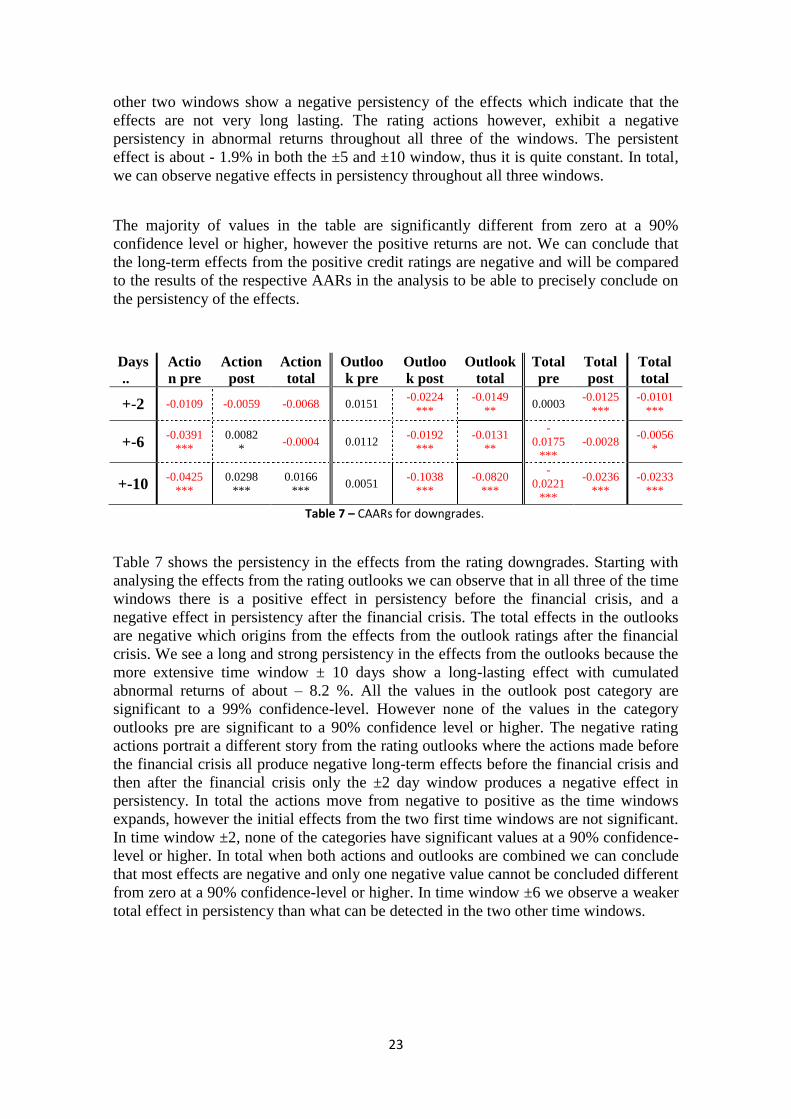
Table 7 shows the persistency in the effects from the rating downgrades. Starting with

analysing the effects from the rating outlooks we can observe that in all three of the time

windows there is a positive effect in persistency before the financial crisis, and a

negative effect in persistency after the financial crisis. The total effects in the outlooks

are negative which origins from the effects from the outlook ratings after the financial

crisis. We see a long and strong persistency in the effects from the outlooks because the

more extensive time window ± 10 days show a long-lasting effect with cumulated

abnormal returns of about – 8.2 %. All the values in the outlook post category are

significant to a 99% confidence-level. However none of the values in the category

outlooks pre are significant to a 90% confidence level or higher. The negative rating

actions portrait a different story from the rating outlooks where the actions made before

the financial crisis all produce negative long-term effects before the financial crisis and

then after the financial crisis only the ±2 day window produces a negative effect in

persistency. In total the actions move from negative to positive as the time windows

expands, however the initial effects from the two first time windows are not significant.

In time window ±2, none of the categories have significant values at a 90% confidence-

level or higher. In total when both actions and outlooks are combined we can conclude

that most effects are negative and only one negative value cannot be concluded different

from zero at a 90% confidence-level or higher. In time window ±6 we observe a weaker

total effect in persistency than what can be detected in the two other time windows.

24

Figure 5 – CAARs for up and downgrades during a 21 day period.

In figure 5 we can see the path of the persistency of the effects from both downgrades

and upgrades. As can be observed, the persistent effects show that both the upgrades

and the downgrades move towards the same negative direction. However it can be

determined that the downgrades show a larger persistency in the effects, which

continues beyond the time window whilst the upgrades stabilizes and even begin to

recover thus not being as persistent as the downgrades.

Figure 6 – CAARs for downgrades post –and pre crisis.

In figure 6 we observe the effects of persistency of the downgrades divided into two

categories. The first one being downgrades before the financial crisis whilst the second

one is downgrades after the financial crisis. As can be observed in figure 6, the

persistency of the effects look very much a like both before and after the financial crisis.

However we can observe a slightly stronger persistency from the downgrades post the

financial crisis, especially after the announcement day.

-0,045

-0,04

-0,035

-0,03

-0,025

-0,02

-0,015

-0,01

-0,005

0

0,005

-10 -9 -8 -7 -6 -5 -4 -3 -2 -1 0 1 2 3 4 5 6 7 8 9 10

Downgrades

Upgrades

-0,05

-0,04

-0,03

-0,02

-0,01

0

0,01

0,02

-10 -9 -8 -7 -6 -5 -4 -3 -2 -1 0 1 2 3 4 5 6 7 8 9 10

Post

Pre

Days

Returns

25

5 ANALYSIS

This section of our research aims to reconnect our empirical results with our theoretical

framework. Recall the aim of this study which is to examine the effects of

up/downgrades on sovereign ratings presented by Moody’s on national stock

exchanges. In order to answer this question we will in this section contrast our results

to previous research and examine eventual deviation and discuss if these could be

explained by theory or not. The following section will be divided into examination of the

AARs, CAARs and the corresponding theory and previous research.

5.1 Aggregated Abnormal Returns

Starting off with the results from the positive outlook announcements made by Moody’s

during the time period preceding the crisis in 2008 we managed to conclude that there

was an overall positive trend in relation to positive announcements. These positive

abnormal returns were however eliminated on the day following the announcement day.

Hence, there is a significant positive effect on stock market returns that could be

explained by outlook announcements made by Moody’s. Examining the action

announcements, the pattern deviates to some extend where there is no significant

excessive return surrounding the announcement day as in the case of an outlook

announcement. On the contrary, there seems to be negative abnormal returns

surrounding the action announcement day. These results go in line with previous

research presented by for example: Hand et al. (1992); Kaminsky et al. (2002) and

Norden et al. (2004). The above-mentioned research also suggested that stock markets

did not react significantly in relation to positive announcements made by CRAs. The

authors did however conclude that stock markets showed significantly negative

abnormal returns in relation to negative announcements. Our results provide a similar

conclusion where outlooks announced post-crisis is negative and highly significant. The

effects pre-crisis are however not negative or significant around the announcement day

of negative announcements. This pattern is however not deviating from previous

observations. Joo et al. (2005) and Pacheco (2012) presented similar results in their

research were effects after the Koran crisis had deeper impact on return than do

previous to the crisis. Our results from action announcements pre- and post the crisis

date further go in line with previous results providing negative abnormal returns in

relation to action announcements made by Moody’s. Hence, our results also provide

patterns suggesting that stock markets do not react significantly to upgrades but react to

negative announcements, especially to outlooks. Another conclusion to be drawn from

our results is that, these already by previous research suggested negative effects, are

enhanced post-crisis. Hence, we suspect that stock markets have become more sensitive

towards announcements made by Moody’s after the crisis of 2008. This reasoning goes

in line with the findings of Joo et al. (2005) and Pacheco (2012).

26

In terms of EMH, we can reject the possibility of our examined markets to be

considered as holding strong forms of market efficiency since we have determined that

there are, at several occasions, has been abnormal aggregated returns that are

significantly certain to have a relation to the announcements made by Moody’s. Since,

this relationship exits, the market is thus not perfectly efficient. The question is rather if

our chosen markets are to be considered to hold weak or semi-strong market efficiency.

What separates them both is, in short, that the weak form do not necessarily include

public information mean whilst the semi-strong form do. This discussion is hard to

determine since we cannot determine what kind of information Moody’s bring in their

announcements. We can only conclude that they do bring new information to markets –

or at least that is what investors believe.

Having established that there are abnormal returns in relation to announcements made

by Moody’s –especially negative ones. We move in to the area of trying to explain these

market anomalies. Recalling how positive announcements had very little effect and not

necessarily significant results amongst our observations. There are two ways of

interpreting these patterns. One way would be to assume that individuals already have

incorporated the positive news which would leave no room for abnormal returns or that

individuals are conservative. Hence, individuals are under-reacting to information and

put trust in their own beliefs and previous experience when they interpret information in

accordance with Thomaidis (2006, p. 9). Negative announcements did however not have

a neutral impact on our examined stock markets and one suggestion could be that

individuals are, in negative scenarios, applying the representativeness heuristics when

incorporating the information. Hence, individuals would let one negative observation

set the tone for all coming negative observations. This would thus have the implication

that if one severely negative announcement was released and realized, this theoretical

viewpoint would suggest that individuals might expect that the next negative

announcement too will have the same severe impact. For example, a downgrade from

the investment grade B to C- would theoretically be worse than a downgrade from AAA

to AA but individuals interpret the event as being equal. Hence, there is a possibility

that severe negative announcements might be influencing other negative announcements

and therefore creating abnormal negative returns. Given the reasoning in regards to how

individuals process information the question arise how individuals capitalize on

information. From the patterns we have observed with no abnormal returns due to

positive announcements and negative abnormal returns due to negative announcements.

We would suggest that the reason for these patterns is due to individuals being loss

averse. That is, individuals are more sensitive to losses than gains and reacts thereafter.

In a positive announcement situation, individuals see no reason to overreact to good

news. But when they are faced with negative ones, they tend to be discouraged to invest

and stock markets fall as suggested by Thomaidis (2006, pp. 7-8)

27

5.2 Cumulative Aggregate Abnormal Returns

In this section the results for the CAARs presented above will be interpreted and

discussed using theory and previous studies as a comparison.

In the results for the upgrades we observed that the persistency of the significant effects

where all negative, this goes against the reasoning of the EMH developed by Fama

(1970). Positive information should create a positive reaction according to the EMH.

We believe that people do not attention the rating upgrades in the long-run thus the

negative reaction are not reactions to the ratings but rather the market going about as

usual. In behavioural finance this reaction could be explained with the help of

conservatism. Conservatism indicates that people value their own expectations and

beliefs more than new information thus these investors will not react to the information

as in this case (Thomaidis, 2006, p. 9). Together with the reaction which we observed

from the AAR where there were some small positive effects we can conclude that in the

longer-run the effects are not persistent. These results are similar to the results from

previous studies in this topic. For example Hand et al. (1992, p. 734) found that rating

upgrades have no effect on the stocks of the stock market. Kaminsky et al. (2002, p.

188) also found results with the same resemblance.

The results for the rating downgrades show a different picture than what the upgrades

show. Almost all the significant results in the downgrades indicate a negative effect in

persistency which goes according to the EMH developed by Fama (1970). Hence with

negative information comes a negative reaction in the effects. This reaction can be

interpreted differently depending on the form of market efficiency of the markets. If the

Markets are in a weak form of market efficiency then the negative ratings could convey

both public information and private information. In a semi-strong form of market

efficiency the negative ratings only convey private information, and finally we can

conclude that a strong from of market efficiency is not present in our study since we do

see a reaction. If a strong from of market efficiency existed then all information would

be incorporated in the price and the ratings could not convey any new information

(Fama, 1970). Another pattern which we observed in the CAARs was that the negative

rating outlooks were more significant than the negative rating actions. One potential

explanation for this could be the fact that outlooks usual are announced before actions

and thus some of the information which actions convey could have already been

conveyed by the outlook. When we compared the result pre and post the financial crisis

in the results we did not see any substantially big differences in persistency of the

effects. However we did see that before the crises there are indications that the

information from the ratings could have been leaked into the market before the

announcement day. After the announcement day we observe that the negative rating

announcements after the crisis have a slightly stronger persistency in the effects than the

ratings before the crisis have. These results show similar results as those found by

28

Norden & Weber (2004, p. 2837-2838), were substantial effects from rating

downgrades were found. Hand et al. (1992, p. 734).also found similar effects on the

American stock market.

The fact that we found a persistency in the effects from downgrades but not upgrades

makes us believe that once again the behaviour of the investor controls the reactions.

We believe that the concept of loss aversion could be an explanation for these results.

People are in general more sensitive to losses than gains therefore negative information

would create a stronger reaction in the minds of the investor than positive information

would. This reaction could occur even if the ratings do not incur any new information,

as long as the investor believes that it does (Thomaidis, 2006, pp. 7-8).

29

6 CONCLUSION

The last section in our research aims to review what we have derived by contrasting our

results toward previous research and our theoretical framework and compare our

conclusion with our research question. This section will start off with a review of our

research question and purpose to show how our conclusions are associated. We will

thereafter elaborate on how our research has contributed to this research area. In the

ending paragraph we give recommendations for further research.

Our research is built on two separate theoretical areas related to the area of CRAs

effects. The theoretical areas we have built our research around are: the market model,

the efficient market hypothesis and behavioral finance. In line with our event study

methodology approach we have aimed to, through usage of established methods and

precious theories, derive our own data in order to examine and conclude:

The effects of up/downgrades on sovereign ratings presented by Moody’s on national

stock exchanges.

Our main purpose with this research is to conclude what effects Moody’s

announcements have on national stock exchanges. Our first sub-purpose is to conclude

if these effects tend to differ pending on if they were carried out pre- or post crisis. Our

second and last sub-purpose is to determine if our examined stock markets are

considered to be perfectly efficient or not. Based on our empirical results we are able to

conclude:

(i) Positive announcements have a small positive effect in the short run but not

in the long run. Negative announcements have a relatively larger negative

effect compared to positive announcements and they tend to persist over

time.

(ii) Negative announcements hold a significantly larger effect post crisis than do

pre and the persistence of the effects are somewhat stronger post crisis.

(iii) Our examined stock markets are according to our results not considered to

hold a strong form of efficiency and should rather be explained as holding a

weak – or semi-strong form. Which one of the latter two is however

inconclusive.

We have contributed to the existing theoretical framework by concluding that the CRAs

announcements have different impact on our chosen segment of stock markets pre – and

post crisis. Thus far, previous research has concluded that CRAs announcements not

only affect bond markets but also stock markets. But, from what we have observed,

there has been no extensive research made which separates the event study into two

separate periods and examined if there are differences in the effects caused by the

announcements made by the CRAs. The research made with a similar approach has only

included one country of choice (see, Joo & Pruitt (2005); Pacheco (2012)) mean whilst

our research includes a larger segment of countries that to larger degree than others

were in debt during our chosen time period. Furthermore, our research presents a,

30

perhaps limited, ground for trying to explain market anomalies that arise due to CRAs

announcements by including behavioural finance.

In regards to further research, we recommend upcoming researchers to further elaborate

on the behavioural financial aspect of why individuals tend to react stronger to e.g.

downgrade announcements than do upgrades. Perhaps a qualitative research approach

would be of interest for this question. Another related topic is if our results are

applicable for the other larger CRAs? Do their announcements provide the same market

reaction or are there any deviations? Including the perspective of pre- and post crisis

would thus examine if some CRAs has increased their influence meanwhile others may

have lost theirs.

31

REFERENCES

Alsakka, Rasha, and Owain Ap Gwilym. "Rating Agencies’ Signals during the

European Sovereign Debt Crisis: Market Impact and Spillovers." Journal

of Economic Behaviour & Organisation 85.2013 (2011): 144-62.

Barberis, N., and R. Thaler. "Chapter 18 A Survey of Behavioural Finance." Handbook

of the Economics of Finance 1 (2003): 1053-128.

Barron, M.J., A.D. Clare, and S.H. Thomas."The Effect of Bond Rating Changes and

New Ratings on UK Stock Returns." Journal of Business Finance &

Accounting 24.3 (1997): 497-509.

Bodie, Zvi, Alex Kane, and Alan J. Marcus.Investments and Portfolio Management. 9th

ed. New York: McGraw-Hill/Irwin, 2011.

Cantor, Richard, and Frank Packer. "Determinants and Impact of Sovereign Credit

Ratings."The Journal of Fixed Income 6.3 (1996): 76-91.

Chen, Nai-Fu, Richard Roll, and Stephen A. Ross. "Economic Forces and the Stock

Market."The Journal of Business 59.3 (1986): 383-403.

Elkhoury Marwan. United Nations. Credit Rating Agencies and Their Potential Impact

on Developing Countries. Rep. Vol. 86. Geneva: United Nations, 2008.

Fama, F. E. "Efficient Capital Markets: A Review of Theory and Empirical Work." The

Journal of Finance 25.2 (1970): 383-417.

Feder, Gershon, and Knud Ross. "Risk Assessments and Risk Premiums in the

Eurodollar Market." Journal of Finance 37.3 (1982): 679-91.

Friedman, Thomas. "NewsHour Online: Thomas Freidman." PBS. N.p., 13 Feb. 1996.

Web.29 Apr. 2013.

<http://www.pbs.org/newshour/gergen/friedman.html>.

Hand, John R.M, Robert W. Holthausen, and Richard W. Leftwich. "The Effect of Bond

Rating Agency Announcements on Bond and Stock Prices." The Journal

of FinanceXI.VII.2 (1992): 733-52.

Holthausen, Robert W., and Richard W. Leftwich. "The Effect of Bond Rating Changes

on Common Stock Prices." Journal of Financial Economics 17 (1986):

57-89.

Joo, S., and S. Pruitt. "Corporate Bond Ratings Changes and Economic Instability:

Evidence from the Korean Financial Crisis." Economics Letters 90.1

(2006): 12-20.

32

Kaminsky, Graciela, and Sergio L. Schmukler. "Emerging Market Instability: Do

Sovereign Ratings Affect Counrty Risk and Stock Returns." Review. The

World Bank Economic Review 2002: 171-95.

Kim, M. K., & Wu, C. (1987). Macroeconomic factors and stock returns. Journal of

Financial Research, 10, 87−98.

La Porta, R., Lopez-de-Silanes, F., Shleifer, A., & Vishny, R. (1997). Legal

determinants of external finance. Journal of Finance, 52, 1131−1150.

MacKinlay, A.C., 1997. Event Studies in Economics and Finance. Journal of Economic

Literature 35, 13–39.

MSCI."About MSCI." MSCI. Web. 15 May 2013. <http://www.msci.com/about/>.

Moody’s."Research & Ratings - Moody's." Research & Ratings - Moody's. Web. 10

May 2013. <http://www.moodys.com/researchandratings>.

Mookerjee, R., and Qiao Yu. "Macroeconomic Variables and Stock Prices in a Small

Open Economy: The Case of Singapore." Pacific-Basin Finance

Journal 5.3 (1997): 377-88.

Nationalencyklopedin."Sterling." Nationalencyklopedin. 2013. Web. 29 Apr. 2013.

<http://www.ne.se/lang/sterling?i_h_word=silver%20sterling>.

Norden, L., and M. Weber. "Informational Efficiency of Credit Default Swap and Stock

Markets: The Impact of Credit Rating Announcements." Journal of

Banking & Finance 28.11 (2004): 2813-843.

Pearce, Douglas K., and Vance Roley. "The Reaction of Stock Prices to Unanticipated

Changes in Money: A Note." The Journal of Finance 38.4 (1983): 1323

-1333.

Peterson, P.P., 1989. Event Studies: A Review of Issues and Methodology. Quarterly

Journal of Business & Economics 28, 36.

Pukthuanthongle, K., F. Elayan, and L. Rose. "Equity and Debt Market Responses to

Sovereign Credit Ratings Announcement." Global Finance Journal 18.1

(2007): 47-83.

Reinhart, Carmen M., and Kenneth S. Rogoff. "From Financial Crash to Debt Crisis."

American Economic Review 101.5 (2011): 1676-706.

Ritter, J. "Behavioral Finance." Pacific-Basin Finance Journal 11.4 (2003): 429-37.

Studenmund, A.H. Using Econometrics: A Practical Guide. 6th ed. N.p.: Pearson

Education, 2011.

33

Thomaidis, Nikos S. The Implications of Behavioural Finance for the Modelling of

Securities Prices. Thesis. University of the Aegean, 2006.

34

Appendix I - Plots

-0,03

-0,02

-0,01

0

0,01

0,02

0,03

-0,06 -0,04 -0,02 0 0,02 0,04 0,06 Re

sid

ual

s

Residual Plot

-0,03

-0,02

-0,01

0

0,01

0,02

0,03

0 20 40 60 80 100 120

Sample Percentile

Normal Probability Plot