The E ff ect of Overcrowded Housing on Children’s Performance at School Dominique Goux (INSEE and ENS) and Eric Maurin (CREST and CEPR) ∗ March 2003 Abstract In France, almost one in five 15 year olds lives in a home with at least two children per bedroom. More than 60% of these adolescents have been held back in primary or middle school, a proportion that is more than 20 points higher than it is on average for adolescents of the same age. This paper develops a semi- parametric analysis that suggests a relation of cause and effect between living in an overcrowded home and falling behind at school. According to our estimations, the disparity in living conditions is a very important channel through which parents’ lack of financial resources affects their children’s schooling. ∗ Corresponding author : Dominique Goux, INSEE, Timbre F230, Division emploi, 18, boule- vard Adolphe Pinard, 75675 Paris Cedex 14, France, e-mail: [email protected], phone: 33 1 41 17 54 42.
Transcript
The Effect of Overcrowded Housing onChildren’s Performance at School
Dominique Goux (INSEE and ENS)and Eric Maurin (CREST and CEPR)∗
March 2003
Abstract
In France, almost one in five 15 year olds lives in a home with at least twochildren per bedroom. More than 60% of these adolescents have been held backin primary or middle school, a proportion that is more than 20 points higherthan it is on average for adolescents of the same age. This paper develops a semi-parametric analysis that suggests a relation of cause and effect between living in anovercrowded home and falling behind at school. According to our estimations, thedisparity in living conditions is a very important channel through which parents’lack of financial resources affects their children’s schooling.
The Effects of Overcrowded Housing onChildren’s Performance at School
1. Introduction
Children from poor families do not do as well and leave school earlier than childrenfrom rich families. These are well-known facts that no longer need to be validated.The interpretation of these facts, however, is still the subject of great controversy.Consequently, public policies that could help reduce inequalities in educationalopportunities remain poorly defined.One basic issue is whether increasing financial aid to the poorest families rep-
resents a good means for improving their children’s performance at school. Anumber of studies argue that parental income, as such, does not have any impacton children’s performance at school. According to these studies, the link betweenpoverty and academic failure is not one of cause and effect. They stress thatincreasing financial aid to poor families would have no effect on the inequalitiesbetween children from rich and poor families.1
Another important issue concerns the impact of targeted aid, aimed to di-rectly improve the living conditions of poor children. Even if financially assistingthe parents of the poorest families would not have any effect on their children’sschooling, aid aimed at specifically improving children’s access to medical care orquality of housing could have a very important and positive effect on children’sdevelopment and performances at school.2
In this paper we try to contribute to this second debate. We focus on one aspectof children’s living conditions, which we suspect to be of particular importance— the amount of personal space they have at home for their activities. Morespecifically, we try to evaluate the impact of the number of persons per room onthe probability of being held back in primary or junior high school. This does notmean measuring the overall effects of parental income, but the effects of a veryparticular potential use of parental income — the spending allotted for housingso that children do not have to live in an overcrowded space. The underlying
1See Mayer (1997), Blau (1999) and Shea (2000).2The absence of a direct effect of parental income on children’s performance does not imply
that an improvement in poor children’s living conditions would not have a positive effect ontheir success at school. The absence of an income effect can just as well mean that the parentsreceiving an income supplement have other priorities than to improve the conditions related totheir children’s success at school.
2
issue is to understand whether public policies favoring quality housing for low-income families could also serve as a vehicle for improving the performances oftheir children and equal opportunities at school.To shed light on this issue, we have used the French Labor Force surveys, which
were conducted each year by the French National Institute for Statistics and Eco-nomic Studies (hereafter, INSEE) between 1990 and 2000. These surveys haveprovided us with large samples of 15 year olds with information on whether theyhave been held back a grade in elementary school or in junior high school, as wellas on how many people there are per room in their home. This dataset makes itpossible to analyze the impact that overcrowded housing has on academic perfor-mances using very large samples of 15-year-old adolescents. We have also used aretrospective survey on schooling and housing conditions during childhood, whichwas carried out by INSEE in 1997. This survey makes it possible to analyze theimpact of having shared a room during childhood on the probability of droppingout of the educational system before earning a diploma.From a methodological viewpoint, the main problem is to estimate the effect of
potentially endogenous regressors (in particular, overcrowded housing) on binarydependent variables (to be or not to be behind at school). In order to solve thisproblem, we have used the semi-parametric estimation method recently developedby Lewbel (2000). This method makes it possible to apply instrumental variabletechniques to non-linear models as easily as to linear models.To implement Lewbel’s technique and identify the causal effect of the housing
conditions, we have consecutively used two different sets of instruments. Thefirst set is constructed from the available information on the sex and month ofbirth of the two oldest children living in the home, as well as on the absolute agedifference between the parents. Families in which the two oldest children are ofthe same sex tend to be more numerous and to live more often in overcrowdedhousing than other families. One of our basic identification assumptions is thatthis is the main channel through which the sex differences between the oldestsiblings actually affect school performances. The second set of instruments isconstructed from the available information on the parents’ place of birth. Parentsborn in urban areas tend - ceteris paribus - to live more overcrowded housing thanparents born in non-urban areas. The identification assumption is that this is themain channel through which parents’ place of birth affect school performances.Standard overidentification tests do not indicate any significant inconsistencies inour different identification hypotheses.Within this framework, our main empirical findings may be summarized as fol-
3
lows. First, a very significant correlation exists between children’s performancesand overcrowded housing. Almost 20% of French adolescents live in a home withat least two children per bedroom. More than 60% of these adolescents have beenheld back a grade in primary or middle school, a proportion more than 20 pointshigher than it is for adolescents in non-overcrowed housing. Secondly, the causaleffect of overcrowding is probably even larger than what the raw correlation sug-gests. The IV estimates of the overcrowding effect are significantly greater thanthe OLS estimates regardless of whether we use instruments built from the infor-mation on the sex and date-of-birth of the oldest siblings or on the parents’ placeof birth. Our data only provide an indirect and potentially rough measurement forhousing conditions. The downward biases that affect the OLS estimates plausiblycorrespond to biases that arise from measurement errors.Lastly, our survey with retrospective information on housing conditions con-
firms that the probability of dropping out of school before earning a diploma issignificantly lower for those who did not share their room during early childhood.All in all, our data provide an array of findings that suggest that overcrowdedhousing is an important way in which parental poverty affects children’s outcomes.The paper is organized in the following way. In the next section, we present an
overview of medical, sociological and sociopsychological literature, which describesthe impact of overcrowded housing on the health and behavior of individuals. InPart III, we develop a model for parental behavior, making it possible to definewhat is meant by the causal impact of overcrowding on school performance, aswell as the econometric strategies that make it possible to identify that impact.In Part IV, we describe the data and methods used, and the econometric resultsare presented in Part V.
2. The Effects of Overcrowded Housing: An Overview ofthe Literature
The sociological and social psychological literature has long been interested inthe problems caused by overcrowded housing 3. Empirically, the degree of over-crowding is measured by the number of persons per room. Theoretically, theproblems caused by lack of living space are conceptualized as the consequences
3Since the 1960s, experiments carried out on groups of rats have brought to light the veryserious behavioral and social problems that occur in animals when the size of their vital livingspace is modified.
4
(a) of an excess of interactions, stimulations and demands from the people livingin the immediate area, and (b) of a lack of intimacy and the possibility of beingalone. People who live in overcrowded housing suffer from not being able tocontrol outside demands. It is impossible for them to have the necessary mini-mum amount of quiet time they need for their personal development. One of themost convincing sociological studies on this subject is perhaps that of Gove et al(1979). Using American data, the authors establish the existence of a very clearcorrelation between the number of persons per room and individuals’ mental andphysical health4.Medical literature has also shown great interest in the health of people living
in overcrowded conditions, i.e. in houses and/or apartments that are too small fortheir families. It has been well established that individuals living or having livedin such conditions are sick more often than others, particularly due to respiratoryinsufficiency and pulmonary problems 5 (Britten et al, 1987, Rasmussen et al,1978, Mann et al, 1992). In general, people who grow up in overcrowded housingdie at a younger age than others (Coggon et al, 1993, Deadman et al, 2001), mostnotably of cancer (Barker et al, 1990).The medical literature gives many reasons for these health problems and their
persistence. Living in an overcrowded space is a source of stress and favorsillnesses linked to anxiety. The members of a family living in a crowded spacealso transmit their infections to one another more easily, weakening their immunesystems. Living in an overcrowded space puts people at greater risk to problemslinked to poor ventilation and hygiene conditions, such as poisoning caused by thesmoking of one or more family members (see the survey by Prescott and Vestbo,1999).
4In addition, the authors establish that the number of persons per room is a good mea-surement for feelings of excessive outside demands and lack of private time. They also showthat the quality of care given to children, and more generally, the quality of the relationshipbetween parents and their children, tends to deteriorate when the number of individuals perroom increases. Gove et al’s (1979) results are obtained from American data, but they comparerather well with Chombart de Lauwe’s (1956) seminal results based on French data, which alsoestablish a statistical relationship between the number of persons per room and the frequencyof social pathologies.
5At greater risk due to unhygienic conditions, they suffer more often than others from appen-dicitis inflammation. According to Coggon et al (1991), the drop in appendicitis inflammationcases observed since the beginning of the 1960s in Anglesey is linked more to the decrease in thenumber of overcrowded housing than to the improvement in the housing’s modern conveniences.In addition, Fuller et al (1993) established a link between the degree of overcrowded housingand the probability of mental health problems through analyzing data from Thailand.
5
With overcrowded housing occupants’ health at greater risk and their capacityfor intellectual concentration being decreased, it is clear that a lack of space is apotentially unfavorable factor for children’s success at school. To our knowledge,however, no study that analyzes the nature and intensity of the links betweenavailable living space and children’s success at school exists in the economic liter-ature. The work published in the sociological and medical literature correspondsessentially to the analysis of statistical correlations. Given that housing andhealth problems probably share common unmeasured determinants, these statis-tical correlations do not necessarily correspond to relations of cause and effect.The meaning of the results obtained from this literature is unclear.In the next section, we will develop an economic model of family behavior that
makes it possible to define what we mean by the causal effect of overcrowdingon children’s performance at school. This model will also help us to defineeconometric strategies that make it possible to identify this effect.
3. Theoretical Framework and Econometric Model
In this section, we develop a model for family behavior that describes the simul-taneous determination of the number of persons per room and the probabilityof academic failure. Our purpose is to define what is meant by the effects ofovercrowding on schooling and to clarify the conditions that make it possible toeconometrically identify this effect. Our model is based on the following assump-tions:(H1) the academic abilities of a child (noted Qi for the child i) depend on the
exogenous characteristics of the child measured in the survey (xi), the character-istics unmeasured in the survey (ui), but also on the total number of children inthe family (Ni) as well as the amount of space available for each member in thefamily home (Li). The underlying assumption is that children do better at schoolwhen they have a quiet room for studying, and have parents who do not have todivide their time between too many children. To stay within a simple framework,we assume that Qi can be log-linearly decomposed,
lnQi = α lnLi + βNi + γxi + ui. (3.1)
(H2) a child experiences academic failure and repeats a grade in elementaryschool and/or middle school if his/her scholastic abilities Qi are lower than aminimum aptitude threshold, which depends only on his/her relative age within
6
his/her age group6 (written ai). The assumption is that at a given level of ability,a child is more vulnerable to being held back if he/she was born at the end ofthe year, meaning that he/she is among the youngest of his/her age group. Innoting Ei as the dummy variable with a value of 1 when the child i is failing, wepostulate that there exists an intercept Q0 and a parameter θ, such that we canwrite:
Ei = 1⇐⇒ lnQi + θai < Q0. (3.2)
(H3) depending on their income (Ri), the number and characteristics of theirchildren, the parents of the child i choose a family consumption level (Ci) andan available space for each person in the family home (Li) in order to maximizea family utility function V (Ci, Li, Qi1, ..., QiNi) subject to the budget constraint:Ci+qL(Ni+2)Li = Ri and the schooling abilities’ production constraint: lnQik =α lnLi+βNi+γxik+uik,where xik and uik characterize the k-th child of the familyi, while qL represents the price per square meter.Assumption (H1) describes how abilities are produced by housing conditions.
Assumption (H2) describes the link between abilities and failure, such as it ismeasured in our data. Assumption (H3) describes how the parents choose betweenspending that improves the family’s living conditions and other forms of spending.In general, the decisions made by the parents lead them to express a housing
demand L = L(R, qL, N, Z, x, u) as a function of income, price, number of children,childrens’ characteristics and factors (denoted Z) which shape their preferences V .With these notations, our purpose is to determine the impact α of Li on academicfailure Ei when Ni, xi, ai and ui are kept constant. Using (3.1) and (3.2), thecorresponding model can be written as:
Ei = 1⇐⇒ α lnLi + βNi + γxi + ai + ui < 0. (3.3)
where the coefficients are normalized so that the impact of the relative age isequal to 1 (i.e., θ = 1). By convention, the intercept Q0 is included in the groupof exogenous variables xi.If the unobserved factors of academic failure ui could be assumed independent
from Li, the identification of α would not cause any particular problem. Theproblem is that these factors are potential determinants of Li. In this scenario,it is unclear whether the correlations observed between Ei and Li reflect the
6In France, two children belong to the same age group (i.e., are in the same year of school)if they were born in the same year.
7
causal effect of Li on Ei, or the fact that the two variables Li and Ei both varysimultaneously with ui. To avoid this kind of problem, it is necessary to observeinstrumental variables that affect the housing conditions Li without determiningacademic failure Ei. Within our theoretical framework, such instruments typicallycorrespond to preference variables that belong to Zi, but are uncorrelated withui. Before describing our econometric strategy in detail, we will develop twoextensions of our basic model.
Extensions of the Basic Model
In the preceding sub-section, we assumed that the available space in the homeL is the only channel by which parental income affects schooling. Let us nowconsider the case where other channels exist (i.e. other kinds of spending F ) thatmake it possible to significantly improve children’s performance at school.
lnQi = α lnLi + βNi + δ lnFi + γxi + ui. (3.4)
Given that Fi is unobserved and potentially determined by the same factorsas Li (namely parental income and preferences), the conditions under which α isidentifiable are not as straightforward as in the previous subsection.For the sake of simplicity, assume that the (log) utility can be written lnV =
ρ(Z 0) lnU(C,L;Z) + (1 − ρ(Z 0) lnQ, where U is an homogenous utility functionwhile Z and Z 0 characterize parents’ preference system. The ρ(Z 0) parameterrepresents the importance given by parents to their children’s development. Underthese assumptions, it is not difficult to check that the demand for inputs can bewritten L(R,Z,Z 0), C(R,Z, Z 0) and F = f(Z 0)R (for more details, see appendixA). Within this framework, equation (3.3) can be rewritten as,
Ei = 1⇔ α lnLi + βNi + γxi + δ lnRi + ai + vi < 0, (3.5)
where vi = ui + δ ln f(Z 0) is a residual that neither depends on R nor on thevariables which belong to Z, but not to Z 0, i.e. the preference parameters whichspecifically determine the trade-off between consumption (C) and the space (L)available for each person in the family home. As a consequence, the identificationof α now requires us (a) to find an instrumental variable z that belongs to Z butnot to Z 0 and (b) to introduce (log) income as a supplementary control variable7
(otherwise R would affect jointly L(R,Z,Z 0) and the residual of the model).
7Let us emphasize that including income as proxy for unobserved inputs would be problematicif we were sticking to an OLS specification. It is indeed very likely that R is not the only source
8
In Appendix A, we also study the case where the quality of housing variesacross the public and private sectors and has an impact on children’s performanceat school. In such a case, it is difficult to identify the effects of overcrowdingwithout at the same time identifying the effects of the housing sector. Thehousing sector being a direct determinant of the price per square meter, it isindeed relatively difficult to justify the existence of an instrument that explainsthe choice of the size of the home without also explaining the choice of the sector.Equation (3.5) has thus to be rewritten in the following way:
Ei = 1⇔ α lnLi + βNi + γxi + δ lnRi + θPubi + ai + vi < 0. (3.6)
where Pubi indicates whether the house belongs to the public (Pubi = 1) orprivate sector (Pubi = 0). The simultaneous identification of α and θ requires (atleast) two instrumental variables. In the empirical application, we will use instru-ments constructed from the available information on the sex and age compositionof the oldest members of the family, as well as on the father’s and mother’s placeof birth.In the preceding sections, we have implicitly considered the total number of
children as an exogenous variable. A perhaps more realistic approach consistsin assuming that parents’ preferences only determine, in an exogenous way, aminimum number of children N0, and that parents choose, in an endogenous way(i.e., in light of the characteristics of the N0 first children), their final number ofchildren Ni
8. Assuming that Ni is endogenous, it is difficult to think of variablesthat would be good instruments for estimating the effects of overcrowded housingwhile not being explanatory factors for the total number of children Ni: everyfactor that determines that families live in a spacious home is also potentially afactor pushing them not to have too many children. Given this reality, it seemsproblematic to estimate the overcrowding effect without estimating at the sametime the family size effect. This is the reason why our models do not focus on thesole overcrowding effect. We always estimate simultaneously the effects of bothfamily size and overcrowded housing 9.
of correlation between L and F .(i.e., very likely that Z∩Z 0 6= ∅). Assuming that some preferenceparameters affect both L and F , the regression coefficient of E on L holding R constant providesa biased estimate of the parameter of interest which is the regression coefficient of E on L holdingF constant.
8In the empirical application, we will limit our analysis to families with at least two children(i.e., such that N0 = 2).
9To evaluate the biases that may arise from errors in the measurement of lnRi, we will also
9
4. Data and Method
The data used for estimating equations (3.3), (3.5 and (3.6) come from the Frenchannual Labor Force Surveys that were carried out between 1990 and 2000. Eachsurvey corresponds to a sample of about 80,000 households, representative of thepopulation of French households (sampling rate 1/300). Each member of thehousehold who is 15 or older is surveyed, with the cut-off age being December 31,of the year preceding the one the survey is conducted. These surveys make itpossible to construct a large sample of 15 year olds (i.e., responding in t, born int− 15), and to analyze the links that exist between their housing conditions andsituations at school.An interesting feature of the French Labor Force Surveys is that only one-third
of the sample is renewed each year. For each t, we can construct a sub-sample ofadolescents born in t− 15 with information on their situation at school at t andt+1. This sub-sample makes it possible to analyze the links between the housingconditions at t and the probability of repeating a grade at t+ 1 (i.e.,being in thesame grade at t and t+ 1).
4.1. Variables
For each 15-year-old respondent, the Labor Force Survey gives (a) their sex, dateof birth and the grade they are in at the time of the survey, (b) the number ofpersons and the number of rooms in their home, (c) their parents’ wages andoccupations (which makes it possible to code their families’ socioeconomic levelusing the French Occupational Prestige Scale), (d) their parents’ age and place ofbirth and (e) the number, sex and birth date of the other children living in thehome. The survey also indicates if the family home belongs to the public sector.Respondents of year t born in t − 15 are in at least the ninth grade if they
have not repeated a year. Thus, our measurement for ”having repeated a grade inelementary school and/or middle school” is simply a dummy variable that equals1 if they are not yet in the ninth grade. For respondents that are tracked for twoyears, our measurement for ”repeating a grade” equals 1 if they are in the samegrade at t and t+ 1.
perform regressions where lnRi is assumed endogenous. We will use the information availableon the head of the household’s and his or her spouses’ fathers’ past occupations as instrumentalvariables. By construction, the past situation of grandparents is correlated with the permanentcomponents of parental income, but uncorrelated with its transitory components (see Maurin,2002).
10
Knowing the number of rooms (NP ) and the number of children (NE), it isalso possible to construct an estimation of the number of children per bedroomfor each home. Assuming that one room is communal and that the parents havetheir own separate bedroom, this estimation can be written as (NP − 2)/NE.Throughout the remainder of the paper, our measurement for overcrowding is adummy equal to 1 when (NP − 2)/NE ≤ 1/2, i.e. when there are at least twochildren per room. Our econometric work has mostly consisted in regressing ourdummy variables for academic failure on this dummy variable for overcrowding10,using family size and family income indicators as control variables.
4.2. Samples
The basic analysis will be carried out using the sample representative of thoseindividuals who were born in t−15, observed in the Labor Force Surveys conductedin t = 1990, ..., 2000, living in two-parent families with at least two children (thebasic instrumental variables are only defined when at least two children are livingin the home). This sample contains about 19, 000 observations. Table 1 presentsthe 15-year-old respondents’ distribution according to the main criteria used inthis paper. We can see that over 17% of adolescents (i.e., 3378/19499) live inovercrowded housing, and that the probability of having repeated a grade is morethan 20 points higher for them (61%) than for others (39.4%). In accordancewith what other studies have already found, the probability of having repeated agrade is higher for boys than girls, for children born at the end of the year thanthose born at the beginning, for the children of large families than those of smallerfamilies, and finally, for the children of poor families than those of rich families.In addition to the Labor Force Surveys, we also used a retrospective survey
conducted in 1997 based on a sample of about 1,000 individuals, representativeof the French male population, aged 20 to 40. The respondents describe theirschooling as well as their housing conditions during childhood. This survey makesit possible to analyze the impact of having had one’s own room during childhoodon the probability of dropping out of school before earning a diploma by applyingeconometric strategies similar to those used to analyze the data from the LaborForce Surveys. Table 2 presents the distribution of the respondents from the 1997retrospective survey according to family size, year of birth, father’s occupation and
10According to this definition, two children and two parents living in a two-room house orapartment or three children and two parents living in a three-room house or apartment areconsidered to be living in overcrowded housing.
11
housing conditions during childhood. This table also describes the variations inthe probability of leaving school without a diploma according to the same criteria.The survey confirms that the probability of not earning a diploma is greater forolder generations than for recent generations, for large families than for those withonly one or two children, and finally, for blue-collar families than for white-collarfamilies. The correlation is also very clear between the housing conditions duringchildhood and the probability of dropping out of school before earning a diploma.Close to 56% of the respondents said that they did not grow up having their ownroom.11 One-third of these individuals dropped out of school before earning adiploma, meaning a rate of academic failure twice that of other children.
4.3. Estimation Method and Instrumental Variables
For the rest of this paper, our purpose will be to identify the parameter α thatappears in equations (3.3), (3.5) and (3.6). If these models were linear, it wouldbe sufficient to observe a set of instrumental variables, i.e. a set of variables thatexplains our endogenous regressors without determining performance at school.With the dependent variable being binary, the observation of such instrumentalvariables is necessary, but not sufficient. A large amount of literature has recentlybeen developed on the supplementary conditions that make it possible to identifythe impact of endogenous regressors on binary dependent variables (see Blundelland Powell, 2000). In this paper, we will use the approach proposed by Lewbel(2000), which is particularly adapted to our problem.In order to identify the effect of an endogenous regressor in a binary choice
model, Lewbel shows that all that is necessary is to observe (in addition to the in-strumental variables Zi) a continuous explanatory variable x0i, which is such thatthe distribution of ui, conditional to the instruments and to the other exogenous
11The retrospective survey on schooling and housing conditions during childhood gives apercentage of individuals who did not have their own room during childhood as almost threetimes greater that the percentage of children living in overcrowded housing estimated from theLabor Force Survey. There are at least two reasons for this. The first one is a generationeffect: most of the respondents of the retrospective survey were 15 years old during the 1980s,while the respondents of the Labor Force Survey were 15 years old during the 1990s. Housesand apartments were made larger from one decade to the other. In addition, the definitionof overcrowding used in the Labor Force Survey is much more restrictive than the one used inthe career survey. As a first approximation, living in overcrowded housing (with the meaningthe word is given in the Labor Force Survey) means that all the children in the home grew upsharing a room with more than one sibling, not just the respondent.
12
regressors, is independent from x0i.12 Once such a regressor x0i and instrumentsZi are made available, Lewbel (2000) shows that the estimation of the impact ofthe endogenous regressors on a binary variable Ei simply requires applying thestandard instrumental variables technique to the following dependent variable LEi
with:
LEi =Ei − I(x0i > 0)
f(x0i/xi, Zi)
where I(x0i > 0) is a dummy variable with a value of 1 when x0i > 0, andf(x0i/xi, Zi) is the density of x0i conditional to the Zi instruments and otherexogenous variables in the model xi.For our case, a natural candidate for x0i is the relative age (denoted ai) of the
adolescent i in his/her age group, i.e. within the cohort of adolescents who wereborn the same year as he/she was. This variable is continuous and it is reasonableto assume that it satisfies the exogenous conditions introduced by Lewbel. Aswe will confirm a little later, this variable is definitely a factor of being held backa year at school: children born at the end of the year — the youngest in their agegroup — are clearly held back much more often than children born at the beginningof the year.As for the instrumental variables, we have used in turn two different sets of in-
struments for identifying the effects of overcrowded housing and family size. Thefirst set is constructed from the information available on the differences in sex andseason-of-birth between the two oldest siblings13 as well as on the absolute agedifference between the parents. These variables describe the basic demographicdifferences between the oldest members of the family. For the group of familieswith at least two children, our data set shows that the families where the two
12It is also necessary that the support of x0 be large and defined in such a way that it contains0. An alternative assumption is that the distribution of very high or very low propensities ofbeing held back (i.e., propensities that are either so high or so low that the probability of beingheld back is either 0 or 1, regardless of x0) is symmetric. See Magnac and Maurin (2002).13Sex and season-of-birth differences between the oldest children have already been used in
other contexts, most notably to identify the effects of family size on mothers’ labor supply(see Angrist and Evans, 1998 or Rosenzweig and Wolpin, 2000). Assuming that mothers’ laborsupply actually belongs in the production function, our estimated impact of family size has to beunderstood as the combination of a direct negative effect (more children implies ceteris paribusless ressources per children) and an indirect positive effect (more children increases the timespent at home by mothers). Within this framework, it is unclear whether we should expect apositive or a negative net effect of family size on performances.
13
oldest children are the same sex tend to be on average bigger (see Appendix B).These families also tend to live in overcrowded housing more often than otherfamilies, especially if the two oldest children were born at different periods of theyear. The impact of the sex differences between the two oldest siblings on the fam-ily size and the housing conditions can be interpreted as reflecting that parentsprefer mixed-gender families and are less reluctant about bringing up two childrenin the same room when they are the same sex14. We will also use an indicatorof the absolute age difference between parents as a supplementary instrument toimprove the precision of our IV estimates (especially when estimating models withthree potentially endogenous regressors). From a technical viewpoint, this instru-mental variable actually contributes to improving the precision of our estimateswhile over-identification tests do not show any significant correlation between thisvariable and the estimated residuals. From a more substantive viewpoint, theimplicit assumption is that the absolute age difference between parents is an indi-cator of parents’ general attitude towards family issues. Parents with a small agedifference are assumed to have more ”modern” preferences, i.e. to place greateremphasis on the quality of their children’s lives rather than on the quantity ofchildren. As a matter of fact, controlling for family income, our data confirm thatparents with a small age difference tend to have less children and to live in lessovercrowded housing than parents with a large age difference.The second set of instruments has been constructed from the available infor-
mation on the mothers’ and fathers’ place of birth. French metropolitan area isdivided into 96 elementary administrative subdivisions (départements). For eachhousehold, the survey provides us with the département where the different mem-bers of the household were born. As shown in Appendix B, significant differencesin family size and housing conditions exist according to these variables.15 Forinstance, mothers born in the Parisian region or in one of the large French citiestend ceteris paribus to have less children than mothers born in less urban areas.We interpret parents’ place of birth as proxies for the housing conditions that par-ents’ have experienced during their early childhood. We interpret the correlation
14Since the month a child was born is a determining factor of his/her repeating a grade, thedifference in the months the oldest children were born determines the difference in the gradethey are in. We interpret the relation between the difference in season-of-birth and overcrowdingas meaning that -ceteris paribus- the parents are less likely to bring up two children together ifthey are in different grades.15We have grouped together the départements, whose impacts on family size and overcrowded
housing were similar. We end up with 6 groups of départements for the mothers’ place of birthand 5 groups for the fathers’.
14
between the parents’ place of birth and current housing conditions as reflectingthe fact that decisions on housing conditions are to some extent determined byearly childhood experience. The identifying assumption is that this is the mainchannel through which parents’ place of birth affects children’s performances.
4.4. The legitimacy of the instruments
We will test the legitimacy of our different instruments using Sargan tests. Oneinteresting feature of Lewbel’s approach is that it makes it possible to test overi-dentification restrictions in non-linear contexts, using the same simple tools as inlinear contexts. Generally speaking, our Sargan tests will not indicate any signif-icant correlation between the estimated residuals and the instrumental variables.Table B3 provides additional evidence of the validity of our basic instrumental
variable, namely the sex differences between the oldest siblings. More specifically,Table B3 shows that the number of hours spent at work by parents and the pro-portion of mothers in the labor force increase significantly with family size, butdo not vary significantly with the sex composition of the oldest siblings. Holdingfamily size constant, there exist no statistically significant differences in the meannumber of hours at work (or in the proportion of mothers out of the labor force)between same-sex families and other families16. Put differently, the sex composi-tion of the oldest siblings has no effect on the amount of time spent at home byparents with their children. Given that this amount of time plausibly representsone of the most important input which is omitted from our schooling-performanceequation, this result means that our basic instrument is not correlated with onepotentially important component of the residual. If we had found a correlationbetween our instrumental variable and this input, we would have been obliged tointroduce this input as a supplementary control variable in the equation. Thiswould have implied a potentially considerable loss in precision.
5. Results
Before moving on to the more sophisticated analysis, we will show our basic find-ings through a simple tabulation. More specifically, Table 3 shows that the proba-bility of being held back a grade is much greater for children living in overcrowdedhousing, regardless of the size and the socioeconomic level of the families under
16We have checked that the same result holds true for our second basic instrument, i.e., thedifferences in season of birth between the oldest children.
15
consideration. For instance, when we focus on relatively ”poor” families, we findthat overcrowding increases the probability of being held back by about 13 points(+29%) in relatively small families, and by about 10 points in relatively largeones (+18%). Generally speaking, there exist almost as many differences in theprobability of being held back between overcrowded and non-overcrowded familiesas there are between poor and rich families or between large and small families.To probe the robustness of these results, we have also performed standard
probit regressions (not reported, see Goux and Maurin, 2001). They confirmwhat the raw statistics suggest: ceteris paribus, adolescents living in a homewith at least two children per bedroom are held back much more frequently thanother adolescents, just as boys are more likely to be held back than girls, andchildren with at least two brothers or sisters are more likely to fall behind thanthose with only one sibling. Within this parametric framework, the overcrowdingeffect is significantly larger than that of children’s sex and than that of familysize. These models also confirm that children born at the beginning of the yearare -ceteris paribus- significantly less often held back than children born at theend of the year 17.
5.1. Overcrowding and the Probability of Being Held Back: A CausalAnalysis
We have estimated several semiparametric models, using Lewbel’s technique andboth OLS and IV specifications. The first kind of model corresponds to equation(3.3) (see Table 4). The dependent variable is a dummy variable with a value of1 when the adolescent has been held back at school. The potentially endogenousexplanatory variables are (a) a dummy variable (Li) with a value of 1 when thereare at least two children per bedroom, (b) a dummy variable (Ni) with a value of1 when there are at least three children living in the home. The Li variable rep-resents our measurement for overcrowding while Ni represents our measurementfor family size. We have added several exogenous regressors to these two poten-tially endogenous variables: the adolescent’s sex, a variable indicating if his orher family lives in the Paris region and a series of variables indicating the surveydate. The date of birth within the year is used as a special auxiliary variable forimplementing our semiparametric estimators.
17A linear regression of the probability of being held back on the different explanatory variablesconfirms this diagnosis: the overcrowding effect is about .11 (i.e. 11 points), i.e. as large as thegender effect (.11) and slightly larger than the family size effect (.09).
16
Model 1 in Table 4 corresponds to our simplest specification. The binarymodel has been linearized using Lewbel’s technique and estimated using the OLSmethod. The results obtained within this framework are quite consistent withwhat raw statistics show. The overcrowding effect is twice as large as that of sexand twice as large as that of family size.The results from this OLS specification are valid under the assumption that
errors in the measurement of overcrowding are negligible and that no unmeasuredfactors simultaneously explain the number of persons per room and the proba-bility of being held back at school. The IV specification (model 2) correspondsto the re-estimation of the OLS model using the generalized method of moments:the dummies for family size and overcrowded housing are considered to be po-tentially endogenous, and their effects are identified using instrumental variablesthat describe the differences in sex and season of birth between the two oldestchildren in the family.This IV model leads to a very strong re-estimation of the overcrowding effect
and a decrease in the number of siblings effect, the latter becoming no longersignificant at standard levels. The IV effect of overcrowding (bα = 0.92) is ninetimes as significant as that of sex. The downward biases that affect the OLSestimates suggest that some unobserved factors simultaneously explain the spaceat home and the performances at school. Our data only provide an indirectand potentially rough measurement for the housing conditions that children haveexperienced during their early childhood. The downward biases that affect theOLS estimates may also correspond to biases that arose from measurement errors.How should a 0.92 estimated impact be interpreted? Given the implicit nor-
malization of our binary models, this result means that the causal impact ofovercrowding is equivalent to 0.92×the impact of a one-year difference in date-of-birth. For poor children living in overcrowded housing, the data show that thedifference in the probability of being held back between children born at the be-ginning of the year and at the end of the year is about 20 points. Thus, accordingto our estimates, the ceteris paribus impact of eliminating overcrowding for thesepoor children is a 18 points (i.e., .92 × 20) reduction in the probability of beingheld back (i.e.,-27%). Table 4 reports the average marginal impact of eliminat-ing overcrowding which is 16.6 percent points when we use the IV specificationcorresponding to model 2.The preceding models implicitely assume that housing is the main channel
through which income affects schooling. They neglect the other potential use ofparental income and potentially overestimate the impact of housing conditions.
17
To address this issue, in the next section, we will re-estimate the housing condi-tions effect by introducing a parental income measurement as a supplementaryregressor18.
5.2. Overcrowded Housing and the Probability of Being Held Back:Estimation of Model (3.5)
Table 5 presents the estimation of equation (3.5). To control for the effects of par-ents’ direct spending on children’s education, a permanent income measurementhas been introduced as a supplementary explanatory variable. This measurementcorresponds to the position of the father’s occupation on the French OccupationalPrestige Scale19.The OLS specification (model 3) confirms the existence of a strong statistical
relationship between the housing conditions and the probability of being held backat school, even when controlling for the father’s socioeconomic status.Model 4 corresponds to the IV re-estimation of model 3 when both the over-
crowding and number of siblings dummy variables are considered as potentiallyendogenous. To improve the precision of the estimator, we have added an indica-tor of the absolute age difference between parents to the set of instruments used forestimating model 3. Sargan tests do not reject the corresponding over-identifyingrestrictions.When compared to model 3, this model leads to a strong (and statistically
significant) re-estimation of the overcrowding effect. In model 4, the overcrowdingeffect (bα = .75) appears seven times greater than the effect of the child’s sex, whilethe two effects are very similar in model 5. Given our normalization choice andgiven the magnitude of the effect of date-of-birth within the year (i.e., 20 points),this result means that eliminating overcrowding for poor children in overcrowededhousing would reduce their probability of being held back by about 15 points (i.e.,.75× 20), meaning a 22% reduction. Table 5 provides the average marginal effectof eliminating overcrowding, which is 13.5 points when we use the IV specificationcorresponding to model 4.
18Given that the instruments used in the previous subsection (sex and season-of-birth dif-ferences between the oldest siblings) are not correlated with parental income, the introductionof income as a supplementary regressor should not have any significant effect on our basic IVresults, however.19For more details on the construction of this variable, see Chambaz et al. (1998). As shown
by Maurin (2002), this variable is actually strongly correlated with family income.
18
Comfortingly, model 4 provides us with results that are not significantly dif-ferent from those of model 2. We end up with similar IV evaluations of the trueeffect of overcrowding regardless of whether we introduce parental income as asupplementary regressor or not. The consistency of our different IV evaluationsmay be interpreted as an indicator of the quality of our identification strategies.Lastly, model 5 corresponds to a re-estimation of model 3 when family per-
manent income is itself considered as potentially endogenous or, at least, poorlymeasured. We have used two dummy variables that indicate if the adolescent’sgrandfathers were managers or professionals (or not) when his or her parents werechildren, as specific supplementary instrumental variables. The results obtainedremain close to model 4. The impact of overcrowded housing remains about sixtimes higher compared to the impact of the adolescent’s sex.
5.3. An Alternative Set of Instrumental Variables
Table 6 proposes a re-estimation of models 4 and 5 using a different set of instru-ments for identifying the impacts of family size and overcrowded housing. Thenew instruments are constructed from the available information on the fathers’and mothers’ place of birth (see Appendix B).Most interestingly, the IV results obtained using these new instruments are not
statistically different from the results obtained using the first set of instruments.The estimated effect of overcrowded housing is significant and large. When familysize, family income and overcrowded housing are all instrumented at once, theestimated impact of overcrowded housing remains about five times higher thanthe estimated impact of the child’s sex (model 9).Model 8 in Table 6 corresponds to the case where we have simultaneously used
the two sets of instruments. The results remain very similar to those from model9 — the overcrowding effect is more than four times higher than the sex effect.Furthermore, the over-identifying restrictions are not rejected by the Sargan test.There is no inconsistency in using instruments constructed from available informa-tion on the place of birth or instruments constructed from available informationon the demographic composition of the (oldest members of the) family.
5.4. An Alternative Dependent Variable
The dependent variable analyzed in the previous subsections is whether a 15-year-old child has ever been held back a grade. This is a cumulative outcome,but the regressors are measured as of the survey date. This raises measurement
19
error problems, which are perhaps only partially overcome by our IV estimationstrategy. In this subsection, we consider the subsample of adolescents, for whichwe have information on their grade at t and t + 1. We focus on the probabilityof repeating a grade at t + 1, i.e. being in the same grade at t + 1 and t. Theinteresting feature of this outcome is that it is non-cumulative and measured afterthe regressors. Table 7 shows that 15 year olds are more likely to repeat a gradewhen they live in an overcrowded home, regardless of the size and income of theirfamily. The probability of repeating a grade is on average 9 points higher (+50%)for 15 year olds living in overcrowded housing.20
Table 8 goes a step further and presents an econometric evaluation of thecausal effect of overcrowding at t on the probability of repeating a grade21 att + 1. Given that repeating a grade at 15 has a different meaning depending onwhether the adolescent has already repeated a grade or not22, we chose to focus onthe subsample of 15 year olds that are on time in their schooling23 at t (N = 5794).This subsample is not representative of the total population of 15 year olds,
and we have to control for the biases that could arise from endogenous selection.The simplest method is to introduce a supplementary control variable, which iscorrelated with the probability of being on time at 15, but uncorrelated with thecurrent probability of moving up to the next grade. To address this issue, wehave used the date-of-birth within the year as a supplementary control variable.The underlying assumption is that the date-of-birth within the year affects theprobability of repeating a grade at early stages in schooling only.24
Given that the date-of-birth within the year is not considered as an exogenousexplanatory factor anymore, it is not possible to implement the Lewbel’s semi-
20Interestingly, the apparent effect of overcrowding on relatively poor 15- year olds seemssmaller than on relatively rich ones. This is due to the fact that the vast majority of relativelypoor adolescents have already been held back a grade.21The minimum age for leaving school being 16, our dependent variable may slightly under-
estimate the actual proportion of adolescents who do not move up to the next grade. Generallyspeaking, it is because of this age limit that our paper focuses on 15 year olds.22Because teachers are required to limit the share of pupils that are two years behind.23An alternative strategy is to consider all adolescents surveyed at t and t+1, to add a dummy
indicating whether they are on time at t as a supplementary explanatory variable and to usethe date-of-birth within the year as an instrumental variable for identifying the effects of beingon time at t. This strategy provides us with similar estimates of the overcrowding effect. Thedrawback of this approach is that it assumes that the effects of overcrowding are the same forchildren who have already been held back as they are for those who have not.24As shown by our previous analysis, it has a strong effect on the probability of being held
back. In this section, we assume that this is an effect on early schooling transitions only.
20
parametric estimator. To overcome this issue, we have relied on a simple linearprobability model, similar to those implemented by Currie and Yelowitz (2001).Table 8 shows the OLS and IV estimations of this linear probability model as wellas the results of a standard probit model.The OLS specification (model 9) confirms that adolescents who live in over-
crowded homes are much less likely to move up to the next grade than otheradolescents, even after controlling for family size and family socioeconomic level.The OLS overcrowding effect (i.e., .08) is larger than the effect of sex and twice aslarge as the effect of family size. The IV effect is not estimated very precisely, butis much larger than the OLS effect. The OLS approach probably underestimatesthe true effect of overcrowding (and overestimates the true effect of family size),but it remains difficult to say exactly by how much.All in all, we come to the same conclusion regardless of whether we focus on
a cumulative or non-cumulative outcome: overcrowded housing is an importantfactor of performance at school and its effect is probably underestimated by naïveregressions, which neglect endogeneity and measurement issues.
5.5. Alternative Measurement for Parental Income
We have re-estimated models 1 through 8 on the sub-sample of adolescents fromfamilies where both parents are wage earners (”wage-earner” sample). This sub-sample contains about 15,000 observations. It is representative of a smaller pop-ulation of adolescents than the ”total” sample, but it has the advantage of givinga direct measurement for parental income. Generally speaking, the results arevery similar to those obtained from the ”total” sample, which is why we have notreported the results. For instance, the overcrowding effect is seven to ten timesgreater than that of the adolescent’s sex (see Goux and Maurin, 2001).We have also re-estimated models 3 through 8 using the two-sample instru-
mental variables technique (TSIV) developed by Angrist and Krueger (1992), andrecently used by Currie and Yelowitz (2000). Again the results have not beenreported, but are available on request. As Angrist and Krueger show, the TSIVestimator is adapted when a potentially endogenous, or poorly measured explana-tory variable, is unavailable in the main sample (in our case, total parental income)even though (a) a group of instrumental variables capable of identifying the effectsof this variable is available in the main sample, (b) an additional survey exists,which gives both the missing endogenous explanatory variable and its potentialinstruments. In our case, the application of this method requires using an ad-
21
ditional survey to get information on the parents’ wage- and non-wage-earningincome, as well as on the instrumental variables used in this paper for identifyingthe effects of the endogenous regressors. We have used a data set that is the resultof the matching of the Fiscal Income Surveys and the Labor Force Surveys carriedout by INSEE in 1997 and 1998. The matching of these surveys is described ingreater detail in Goux and Maurin (2001). This matching makes it possible toconstruct a sample that is representative of the total population of households,for which we know the total income (thanks to the Fiscal Income Surveys), andall the instrumental variables (thanks to the Labor Force Surveys). To test theconsistency of our different approaches, we separately estimated a specific incomeeffect for families with at least one non-wage earner and a specific income effectfor wage-earning families (for which we have a direct income measurement).The results obtained using this method are in accordance with those given
in table 5. According to our TSIV estimator, growing up with several childrenper bedroom increases the probability of falling behind at school in proportionscorresponding to about nine times the difference that exists between girls andboys. Comfortingly, we find about the same income effect for wage-earning andnon-wage-earning families.
5.6. Overcrowded Housing and the Probability of Falling Behind: Es-timation of Model (3.6)
To complete our analysis, we re-estimated the preceding models by introducinga dummy variable, whose value is 1 when the family lives in public housing (i.e.,[Public=1]), as a supplementary explanatory variable (Table 9). This meansestimating equation (3.6) and testing the assumption that it is not overcrowdedhousing in itself that causes academic failure, but the sector in which the over-crowded housing is situated.When we consider the dummy variable [Public=1] as exogenous (see models
11 and 12),25 its addition only marginally modifies the results from models 3 and4. Once the effects of overcrowding, family size and parental income are takeninto account, we only observe a very slight academic success differential betweenchildren living in public housing and the others. The high rate of academic failurethat children from public housing experience reflects above all the poverty of their
25This is the case when all eligible households apply in order to obtain public housing andwhen the access to such housing is mostly a matter of income and luck.
22
families and their overcrowded living space.26
When considering the choice of living in public housing as endogenous (models13 and 14), the results are less precise, but continue to suggest that overcrowdedhousing in itself has a considerable impact on schooling.27 The effect of livingin public housing is three times smaller than the overcrowding effect, and notsignificantly different from zero at standard levels.
6. Single Room and Diploma
Table 10 presents the estimations carried out using the survey on schooling ca-reers conducted in 1997. The advantage of this survey is that it gives more directinformation on respondents’ housing conditions during their childhood and makesit possible to identify the potential long-term effects on educational achievement.The dependent variable indicates if the individual dropped out of school beforeearning a diploma, while the central independent variable indicates if the individ-ual had his or her own room at the age of 11. The disadvantage of this surveyis that it is much smaller than the Labor Force Surveys and does not allow foras precise an identification of the structural parameters. When we restrict theanalysis to the individuals who had at least one brother or sister, the sample onlycontains a little over 600 individuals.These supplementary investigations tend, however, to confirm the diagnosis
obtained using the Labor Force Surveys. The parametric specification showsthat -controlling for the father’s occupation and the number of siblings- individualswho have their own room during childhood had a much smaller probability thanthe others of dropping out of school before earning a diploma (model 15). UsingLewbel’s semiparametric technique (with age as the auxiliary variable) and anOLS specification, we obtain the same basic results (model 16). The overcrowdingeffect is as strong as the effect of family size.Using Lewbel’s technique and an IV specification, we obtain results which are
not very precise, which is not surprising given the small size of the sample (model17). They suggest, however, that the true effect of housing conditions on theprobability of dropping out of school before earning a diploma is undoubtedlyhigher than the effect estimated by the maximum likelihood or OLS techniques.
26These results go in the same direction as those recently obtained by Currie and Yelowitz(2000) using American data.27The diagnosis is similar when we re-estimate models 10 through 16 by adding Public=1 as
an endogenous regressor.
23
The estimated IV effect is 16 times greater than the effect of being one year older.The probability of dropping out of school before earning a diploma decreases byapproximately 1/3 of a point per year (in our sample). This means that thosewho have their own rooms have a probability of dropping out of school that is onaverage about five points less than the others.
The differences between the OLS and the IV estimates are of the same magni-tude as those obtained using the Labor Force Surveys in the previous subsections.Whether analyzing the probability of repeating a year or the probability of drop-ping out of school before earning a diploma, the raw effects definitely seem tosystematically underestimate the causal effect of housing conditions.
7. Conclusion
Several results have come from our analysis. First, we found a very clear corre-lation between housing conditions during childhood and performance at school.Children who grow up in a home with at least two children per bedroom areboth held back and drop out of school before earning a diploma much more oftenthan other children. Second, we showed that this correlation between housingconditions and academic failure can only partially be explained by differences inincome and the number of children between families. Ceteris paribus, childrenwho grow up sharing a room with at least one sibling fall behind at school muchmore often than other children. Lastly, we developed a semi-parametric analysisthat suggests that the link between housing conditions and academic failure is oneof cause and effect. Altogether, we have an array of findings that indicate thatpublic policy favoring the access of modest households to larger dwellings couldhave a substantial effect on educational inequalities.Further research is necessary to really define a housing policy that could affect
the poorest children’s school performance. This research must rely on in-depthanalysis of the effects of existing public policies that favor the housing of low-income families.
References
[1] Angrist J. and W. Evans, 1998, Children and their Parents’ labor Supply:Evidence from Exogenous Variations in Family Size, American EconomicReview, 88:450-477.
24
[2] Angrist J. and A. Krueger, 1992, The Effect of Age at School Entry on Educa-tional Attainment: An Application of Instrumental Variables with Momentsfrom Two Samples, Journal of the American Statistical Association, 418:328-336.
[3] Barker D.J., D. Coggon, C. Osmond and C. Whickham, 1990, Poor housingin childhood and high rates of stomach cancer in England and Wales, BritishJournal of Cancer, 61(4): 575-578.
[4] Blau D., 1999, The Effect of Income on Child Development, The Review ofEconomics and Statistics, LXXXI (2): 261-277.
[5] Blundell R. and J. Powell, 2000, Endogeneity in Nonparametric and Semi-parametric Regression Models, Communication for the 8th World Congressof the Econometric Society.
[6] Britten N., J.M. Davies and J.R. Colley, 1987, Early Respiratory Experienceand Subsequent Cough and Peak Expiratory Flow Rate in 36 year Old Menand Women, British Journal of Medicine, 294: 1317-20.
[7] Chambaz C., E. Maurin and C. Torelli, 1998, L’évaluation sociale des profes-sions en France, Revue Française de Sociologie, 39(1): 177-199.
[8] Chombart de Lauwe P.H., 1956, La vie quotidienne des familles ouvrières,Paris: CNRS.
[9] Coggon D., D.J. Barker, M. Cruddas and R.H. Olivier, 1991, Housing andAppendicitis in Anglesey, Journal of Epidemiology and Community Health,45: 244-6.
[10] Coggon D., D.J. Barker, H. Inskip and G. Wield, 1993, Housing in earlylife and later mortality, Journal of Epidemiology and Community Health, 47:345-348.
[11] Deadman D.J., D. Gunnel, G.D. Smith and D. Frankel, 2001, Childhoodhousing conditions and later mortality in the Boy Orr cohort, Journal ofEpidemiology and Community Health, 55: 10-15.
[12] Currie J. and A. Yelowitz, 2000, Are Public Housing Projects Good for Kids?Journal of Public Economics, 75: 99-124.
25
[13] Fuller T.D, J.N. Edwards, S. Sermsri and S. Vorakitphokatorn, 1993, Hous-ing, stress, and physical well-being: evidence from Thailand, Social ScienceMedicine, 36 (11): 1417-1428.
[14] Goux D. and E. Maurin, 2001, The Impact of Overcrowded Housing on Chil-dren’s Performances at School, Unpublished manuscript, CREST, Malakoff.
[15] Gove W. , M. Hughes and O. Galle, 1979, Overcrowding in the Home: AnEmpirical Investigation of its Possible Pathological Consequences, AmericanSociological Review, 44: 59-80.
[16] Lewbel A., 2000, Semiparametric Qualitative Response Model Estimationwith Unknown Heteroscedasticity or Instrumental Variables, Journal ofEconometrics, 97: 145-177.
[17] Magnac T. and E. Maurin, 2002, Identification and Information in MonotoneBinary Models, Unpublished Manuscript, CREST, Malakoff.
[18] Mann S.L., M.E. Wadsworth and J.R. Colley, 1992, Accumulation of factorsinfluencing respiratory illness in members of a national birth cohort and theiroffspring, Journal of Epidemiology and Community Health, 46: 286-292.
[19] Maurin E., 2002, The Impact of Parental Income on Early Schooling Tran-sitions: A Reexamination using Data over Three Generations, Journal ofPublic Economics, vol:85, pp: 301-332.
[20] Mayer S., 1997, What Money Can’t Buy: Family Income and Children’s LifeChances, Cambridge MA: Harvard University Press.
[21] Prescott E. and J. Vestbo, 1999, Socioeconomic status and chronic obstruc-tive pulmonary disease, Thorax, 54: 737-741.
[22] Rasmussen F.V., L. Borchsenius, J.B. Winslow and E.R. Ostergaard, 1978,Associations between housing conditions, smoking habits and ventilatory lungfunction in men with clean jobs, Scandinavian Journal of Respiratory Disease,59: 264-76.
[23] Rosenzweig M. and K. Wolpin, 2000, Natural Experiment in Economics,Journal of Economics Literature, 38(4) :827-874.
[24] Shea J., 2000, Does Parents’ Money Matter ?, Journal of Public Economics,77: 155-184.
26
Appendix A
We assume that Qi depends not only on xi, ui, Ni, Li, but also on some ofthe expenses of children’s education and development Fi. Under this assumption,equation (3.1) can be rewritten:
lnQi = α lnLi + βNi + δ lnFi + γxi + ui. (7.1)
and parents maximize:lnVi = (1− ρ(Z2i)) lnU(Ci, Li, Z1i)+
ρ(Z2i)(αNi lnLi + δNiPk=1
lnFik)
subject to: Ci + qL(Ni + 2)Li + qFNiPk=1
Fik = Ri.
Within this framework, the optimal level of expenses Fi is the same for allchildren and the first-order conditions can be written:
(1− ρ(Z2i))U0C
U= λ,
(1− ρ(Z2i))U0L
U+ ρ(Z2i)α
Ni
Li= λqL(Ni + 2),
ρ(Z2i)δFi= λqFNi.
where λ represents the Lagrange multiplier. Assuming that U is homogenousof degree υ, we have U
0CC + U
0LL = υ and the first-order conditions implies λ =
The interesting point is that the share of educational expenses in total incomefi(Ni, Z2i) varies with Ni and Z2i, but not with the Z1i variables, i.e. with thevariables that specifically determine the trade-off bewteen Ci and Li.Within thisframework, the equation determining educational outcome can be rewritten,
Ei = 1⇔ α lnLi + βNi + γxi + δ lnRi + ai + vi < 0,
where the new residual vi = ui+δ ln(fi) is uncorrelated with the Z1i variables.Asa consequence, the effect of lnLi on the probability of being held back can beidentified by introducing lnRi as a supplementary control variable an by usingZ1i variables as instruments.
27
Let us now assume that there exists two sectors A and B, such that the priceof housing is lower in A than in B (i.e., qLA < qLB), but such that A is only forlow-income families (i.e., only when Ri < R0) and such that living in A implies anon-positive impact φ on children’s development, meaning:
where Pubi is a dummy variable with value 1 when the housing is in A.Within this framework, the educational expenses ( Fi = fiRi) do not depend
on the sector chosen by the family. In contrast the optimal level of consumptionand housing size depends on the sector. More specifically, given the homogeneityof U , when the family chooses k, the optimal consumption and housing size canbe written as:
C∗ik = ci(qLk)((1−Nifi)Ri)1/(ν(1−ρi)+ρiNiα),
L∗ik = li(qLk)((1−Nifi)Ri)1/(ν(1−ρi)+ρiNiα),
and family i chooses A, if and only if:(1− ρ(Z2i) ln
U(c∗Ai,l∗Ai,Z1i)
U(c∗Bi,l∗Bi,Z1i)
+ ρ(Z2i)Ni(α lnl∗Ail∗Bi− φ) > 0,
where c∗ki represents ci(qLk) and l∗ki represents li(qLk), which can be rewrittenas:
φ <(1− ρ(Z2i)
ρ(Z2i)Niln
U(c∗Ai, l∗Ai, Z1i)
U(c∗Bi, l∗Bi, Z1i)
+ α lnl∗Ail∗Ai
(7.3)
This inequality simply means that eligible families choose A if and only if thenegative direct impact on children’s development φ is smaller than the positiveimpact on welfare, implied by the lower housing price.Functional forms exist such that (when φ is sufficiently small) condition (7.3)
is always true and eligible families all apply for housing in A. In such a case, thechoice of housing sector only depends on income (eligibility condition). Once wecontrol for the income effect, omitting Pubi from our models does not generatespecific endogeneity biases.In general, the choice of A depends not only on Ri, but also on Z1i and Z2i.
In such a case, the Pubi variable is an endogenous determinant of performance atschool, and it potentially has the same determinants as Li.
28
30
Appendix B
Table B1: Correlation between the Differences in Sex and Date of Birth of the Oldest Members of the Family and the Potentially Endogenous Explanatory Variables
Girl + Girl Ref. Ref. Ref. Difference in quarters of birth between the two oldest siblings
-0.04 (0.01) -0.00
(0.01)
0.01 (0.01)
Absolute difference in parents’ age
<2 years -0.51 (0.03)
-0.33 (0.02)
0.31 (0.01)
2-5 years -0.38 (0.03)
-0.26 (0.02)
0.19 (0.02)
>5 years Ref. Ref. Ref. Father’s father = manager or professional
-
-
0.89 (0.03)
Mother’s father = manager or professional
- -
0.72 (0.03)
Number of Observations 19499 19499 19499 Source : Labour Force Surveys, 1990 to 2000, Insee. Field « Total » sample : Children who were born in t-15 and surveyed in t living in an intact family with two or more children.
31
Table B2: Correlation between Parents’ Places of Birth and the Potentially Endogenous Explanatory Variables
Potentially endogenous regressors
[Overcrowded Housing=1] [Nb siblings>2]
Intercept -.55 (.02)
1.08 (0.06)
Mother’s place of birth Parisian suburbs Ref. Ref.
Paris and large cities -.84 (.08)
-.35 (.06)
Regions M1 -.52 (.07)
-.38 (.06)
Regions M2 -.73 (.09)
-.54 (.07)
Regions M3 -1.12 (.06)
-.66 (.05)
Regions M4 -1.81 (.15)
-.72 (.07)
Father’s place of birth Parisian suburbs Ref. Ref.
Paris and large cities -.81 (.07)
-.45 (.06)
Regions P1 -.59 (.08)
-.44 (.06)
Regions P2 -.89 (.06)
-.61 (.05)
Regions P3 -1.47 (.10)
-.45 (.06)
Number of Observations 19,499 19,499 Source : Labour Force Surveys, 1990 to 2000, Insee. Field « Total » sample : Children who were born in t-15 and surveyed in t living in an intact family with two or more children. Definition of the dummies indicating mother’s place of birth: Parisian suburbs correspond to departments 92, 91, 78, 93, 94, 95, 77; Paris and large cities correspond to departments 75, 59, 60, 13, Regions M1 correspond to departments 06, 11, 14, 20, 24, 28, 32, 37, 41, 52, 53, 55, 58, 62, 76, 80, 83, 89, 97, Regions M2 correspond to departments 04, 15, 16, 23, 33, 35, 46, 61, 72, 74, 79, 84, Regions M3 to departments 01, 29, 40, 43, 51, 54, 73, 82, 81, Regions M4 correspond to the remaining departments. Definition of the dummies indicating father’s places of birth: Parisian suburbs correspond to departments 92, 91, 78, 93, 94, 95, 77, Paris and large cities correspond to departments 75, 59, 60, 13, Regions P1 correspond to 05, 06, 11, 24, 28, 47, 52, 53, 62, 68, 80, 89, 97, Regions P2 correspond to departments 01, 07, 18, 25, 26, 29, 31, 42, 4, 47, 50, 51, 56, 85, and Regions P3 to remaining departments.
32
Table B3: Average number of hours spent at work per week by parents and proportion of mothers out of the labour force,
by family size and sex differences between the oldest siblings
Nb of children and sex differences between oldest
siblings
Average number of hours spent at work
(per week) by
Proportion
mothers out of the labor force
(%) Mothers Fathers Mothers+Fathers
Two Children Same sex 34.6 43.0 67.4 19.7 Different sex 34.8 43.2 67.6 20.6 Three Children Same sex 32.2 43.0 60.3 36.8 Different sex 31.5 43.1 60.7 34.3 Four children or more
Same sex 30.6 41.7 50.6 64.3 Different sex 30.7 41.6 49.7 65.5 Source: Labor Force Surveys, 1990 to 2000, Insee. Reading: Consider intact families with three children and such that the two oldest children are same sex. 36.8% of the mothers are out of the labor force. The average number of hours worked by fathers (mothers) is 43.0 (32.2).
33
Table 1: The Labour Force Surveys’ Samples: Basic Statistics
Number of Observations
Proportion held back (%)
Gender
Male 10080 48.4 Female 9419 37.5
Family size 1 or 2 children 8723 34.9 3 or more 10776 49.8
Total 19,499 43.1 Source : Labour Force Surveys, 1990 to 2000, Insee. Field « Total » sample : Children who were born in t-15 and surveyed in t living in an intact family with two or more children. Note: Family socio-economic level correspond to father’s position on the French occupational prestige scale (Chambaz et al., 1998).
34
Table 2: The Survey on Educational and Occupational Career (1997) : Basic Statistics
Respondents with one or more sibling
Number of Observations % without diploma
Family size : 3 or more siblings 359 32.6 1 or 2 276 18.9 Date of birth :
Born after 1964 357 23.5 Born before 1964 258 31.8 Father’s occupation :
Own Room at 11 274 18.9 No Own Room 341 33.4 Total 615 26.9
Source: Survey on Educational and Occupational Career, 1997, INSEE.
35
Table 3: Overcrowded Housing and the Probability of Being Held Back: Basic Facts
in % Overcrowded
housing Non overcrowded
housing
Relatively poor families
Siblings>2 68.1 58.4
Siblings=2 56.9 44.5
All 65.7 52.6
Relatively rich families
Siblings>2 58.1 32.2
Siblings=2 36.1 26.8
All 49.5 29.3
All families
Siblings>2 65.7 45.1
Siblings=2 47.9 33.4
All 61.0 39.4
Source : Labour Force Surveys, 1990 to 2000, Insee. Field: Children who were born in t-15 and surveyed in t living in an intact family with two or more children. Note: Relatively rich (poor) families are families which socio-economic level is above (below) the median of the distribution. Reading : The probability of being held back is 68.1% in relatively poor, large and overcrowded families. In relatively rich, small and non-overcrowded families, the probability of being held back is 29.3%.
36
Table 4: The Impact of Overcrowded Housing on the Probability of being Held Back. An Estimation of Equation (3.3)
Semiparametric binary models
OLS IV
(1) (2) Overcrowded housing 0.20
(0.01) 0.92
(0.24)
Number of siblings >2
0.11 (0.01)
-0.09 (0.07)
Male
0.10 (0.01)
0.10 (0.01)
Mean marginal effect of overcrowding on the prob. of being held back (percent point)
+3.6
+16.6
Number of Observations 19 499 19 499
Sargan Statistic (p)
- 4.5 (.11)
Source : Labour Force Surveys, 1990 to 2000, Insee. Field : Children born in t-15, surveyed at t, living in an intact family with at least two children. Note : The dependent variable corresponds to a dummy variable with value 1 when the child is behind at school. The regressions correspond to the implementation of Lewbel’s semiparametric estimators with the date of birth within the year as an auxiliary variable. In the IV model, the dummy with value 1 when the housing is overcrowded and the dummy with value 1 when the number of children is greater or equal to 3 are assumed endogenous. The instruments are (a) three dummies indicating whether the two oldest siblings are two girls, two boys, one girl and one boy, (b) a variable which takes the values 0, 1 or 2 depending on the difference in quarters of birth between the two oldest siblings. The models also include an intercept, ten dummies indicating the date of survey and one dummy indicating whether the household is in the Paris region as supplementary exogenous regressors.
37
Table 5: The Impact of Overcrowded Housing on the Probability of Being Held Back. An Estimation of Equation (3.5)
Semiparametric binary models
OLS IV IV
(3) (4) (5)
Overcrowded Housing 0.11 (0.01)
0.75 (0.28)
0.61 (0.37)
Number of Siblings>2 0.08
(0.01) -0.24 (0.20)
-0.20 (0.21)
Socio-economic Status
-0.14 (0.01)
-0.10 (0.02)
-0.13 (0.05)
Male 0.10
(0.01) 0.10
(0.01) 0.10
(0.01)
Mean marginal effect of overcrowding on the prob. of being held back (percent point)
+2
+13.5
+11
Number of Observations 19499 19499 19499
Sargan Statistic (p)
- 4.3
(0.36) 4.3
(0,50) Source : Labour Force Surveys, 1990 to 2000, Insee. Field : Children born in t-15, surveyed at t, living in an intact family with at least two children. Note : Same dependent variable, estimation techniques and non-reported independent variables as in table 4. In model (4), the dummy variable with value 1 when the housing is overcrowded and the dummy variable with value 1 when the number of children is greater or equal to 3 are assumed endogenous. In model (5), we assume that the socio-economic status is endogenous too. In model (4) we use the same instrumental variables as in model (2) as well as two dummies indicating whether the absolute age difference between the father and the mother is less than two years or between two and five years. In model (5), we use a set of dummies indicating whether the grand-fathers were managers and/or professionals as supplementary instrumental variables
38
Table 6: The Impact of Overcrowded Housing on the Probability of Being Held Back : A Re-estimation of Equation (3.5) using an Alternative Set of Instruments
Semiparametric binary models
IV IV IV
(6) (7) (8)
Overcrowded Housing 0.57 (0.15)
0.48 (0.20)
0.43 (0.17)
Number of Siblings>2 -0.24
(0.18) -0.20 (0.18)
-0.15 (0.14)
Socio-economic Status
-0.12 (0.01)
-0.15 (0.03)
-0.16 (0.03)
Male 0.10
(0.01) 0.10
(0.01) 0.10
(0.01)
Marginal effect of overcrowding on the prob. of being held back (percent point)
+10.2
+8.7
+7.8
Number of Observations 19,499 19,499 19,499
Sargan Statistic (p)
9.3 (0.23)
9.3 (0.32)
11.2 (0,42)
Source : Labour Force Surveys, 1990 to 2000, Insee. Field :Children born in t-15, surveyed at t, living in an intact family with at least 2 children. Note : Same dependent variables, estimation techniques and non-reported independent variables as in table 4. In model (6), the dummy variable with value 1 when the housing is overcrowded and the dummy variable with value 1 when the number of children is greater or equal to 3 are assumed endogenous. In model (7) and (8), we assume that the socioeconomic status is endogenous too. In model (6) we use a set of five dummies indicating mother’s place of birth and a set of four dummies indicating father’s places of birth as instrumental variables. In model (7) we use a set of dummies indicating whether the grand-fathers were managers and/or professionals as supplementary instrumental variables for identifying the effect of the socio-economic status. In model (8) we add the sex and season of birth differences between siblings and the absolute age difference between parents as supplementary instrumental variables
39
Table 7: Overcrowded Housing and the Probability of Repeating a Grade: Basic Facts
in % Overcrowded
Housing Non-overcrowded
housing
Relatively poor families
Nb Siblings>2 33.0 28.7
Nb Siblings=2 27.2 25.0
All 31.7 27.1
Relatively rich families
Nb Siblings>2 31.7 18.1
Nb Siblings=2 24.8 17.4
All 28.8 17.8
All families
Nb Siblings>2 32.7 23.2
Nb Siblings=2 26.2 20.3
All 30.8 21.7
Source : Labour Force Surveys, 1990 to 2000, Insee. Field: Children who were born in t-15 and surveyed in t and t+1, living in an intact family with two or more children. Note: Relatively rich (poor) families are families which socio-economic level is above (below) the median of the distribution of permanent income. Reading : The probability of repeating a grade is 33% in relatively poor, large and overcrowded families. In relatively rich, small and non-overcrowded families, the probability of repeating a grade is 17.8%.
40
Table 8: An Alternative Dependent Variable : the Impact of Overcrowded Housing on the Probability of Repeating a Grade
Linear Probability Model
OLS (9)
IV (10)
Overcrowded Housing .08 (.02)
.48 (.22)
Number of Siblings>2 .04 (.01)
-.14 (.17)
Socio-economic Status
-.09 (.01)
-.07 (.01)
Male .06 (.01)
.06 (.01)
Date of Birth -.002 (.002)
-.001 (.002)
Number of Observations 5,794 5,794
Sargan statistic (p)
2.9 (.81)
Source : Labour Force Surveys, 1990 to 2000, Insee. Field : Children born in t-15, surveyed at t and t+1, on time at school and in an intact family with at least two children at t. Note : The dependent variable is “to be in the same grade at t and t+1“ . Models 9 and 10 correspond to the OLS and IV linear regression of this dependent variable on the explanatory variables. The IV model assumes that both the family size and the overcrowded housing indicators are endogenous. The instruments correspond to the sex and season-of-birth differences between the two oldest siblings, the absolute age difference between parents and indicators of the places of birth of the two parents.
41
Table 9: The Impact of Overcrowded Housing on the Probability of Being Held Back: An Estimation of Equation (3.6)
Semiparametric binary models
OLS IV IV IV
(11) (12) (13) (14)
Overcrowded Housing 0.10 (0.01)
0.49 (0.12)
0.44 (0.20)
0.35 (0.21)
Number of Siblings>2 0.07 (0.01)
-0.20 (0.12)
-0.22 (0.13)
-0.17 (0.13)
Socio-economic Status
-0.13 (0.01)
-0.11 (0.01)
-0.11 (0.01)
-0.15 (0.03)
Male 0.10 (0.01)
0.10 (0.01)
0.10 (0.01)
0.10 (0.01)
Public=1 0.10 (0.01)
0.07 (0.02)
0.15 (0.25)
0.11 (0.24)
Marginal effect of overcrowding on the prob. of being held back (percent point)
+1.8
+8.8
+7.9
+6.3
Number of Observations 19499 19499 19499 19499
Sargan Statistic (p)
- 15.9
(0.25) 15.9
(0.25) 14.7
(0.33) Source : Labour Force Surveys, 1990 to 2000, Insee. Field : Children born in t-15, surveyed at t, living in an intact family with at least two children. Note : Models (11) and (12) correspond to a re-estimation of models (3) and (4) with (Public=1) as a supplementary exogenous regressor. Model (13) corresponds to a re-estimation of model (12) when (Public=1) is considered as potentially endogenous. In model (14), family socio-economic status is considered as endogenous too. The instruments used for identifying the effect of overcrowding, family size and public housing are the following: sex and season-of-birth differences between oldest siblings, absolute age difference between parents, parents’ places of birth. Family socio-economic status is instrumented with the same instruments as those used in model (7).
42
Table 10: The Effect of Having Ones Own Room at 11 on the Probability of Leaving School without Diploma
Parametric
Model
Semiparametric models
Probit OLS IV
(15) (16) (17)
Intercept
2.32 (0,6)
-4.4 (1.3)
-0.2 (0,9)
Own Room at age 11 -0.58 (0.20)
-1.7 (1.3)
-16.0 (14.3)
Number of siblings >2
0.45 (0.19)
-1.8 (1.3)
-19.6 (21.1)
Father=Manual Worker
0.54 (0.20)
2.9 (1.3)
2.8 (3.0)
Father= Manager/Professional
0.19 (0.37)
1.6 (2.4)
0.4 (4.0)
Age 0.76 (0.43)
- -
Number of observations 632 632 632
Sargan Statistic (p)
- 1.24 (0.87)
Source : Survey on Schooling and Occupational Career, 1997, Insee. Field : Men, age 20-45, with at least one sibling. Note The dependent variable corresponds to a dummy with value 1 when the individual has not earned any diploma before leaving school. Model (15) is a standard Probit model while models (16) and (17) are semiparametric models, estimated using Lewbel’s technique, the date of birth being used as an auxiliary variable. Model (16) corresponds to an OLS specification, models (17) to an IV specification. In model (17), two regressors are assumed potentially endogenous : the dummy variable with value 1 when the individual had a room of his own when he was 11, and the family size indicator. The instrumental variables are : (a) three dummies indicating whether the two oldest siblings are two girls, two boys, one girl and one boy, (b) two dummies indicating whether the absolute age difference between the father and the mother is less than two years or between two and five years, (c) a variable which takes the values 0, 1 or 2 depending on the difference in quarters of birth between the two oldest siblings.


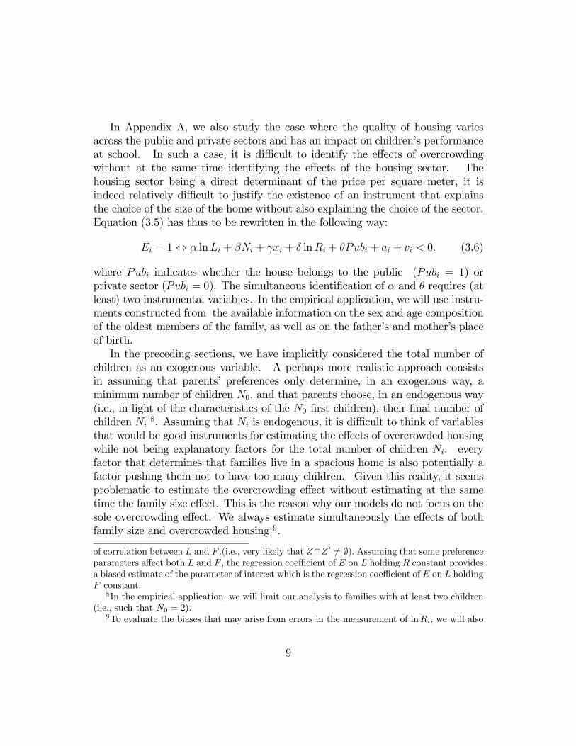


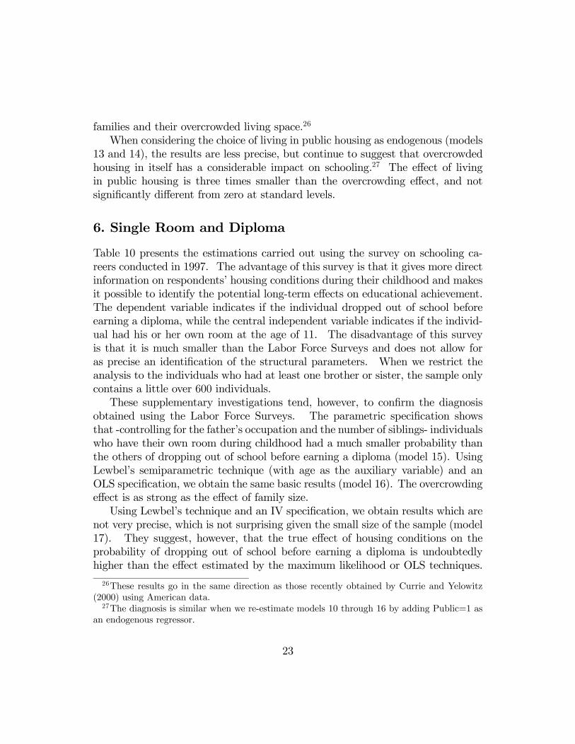


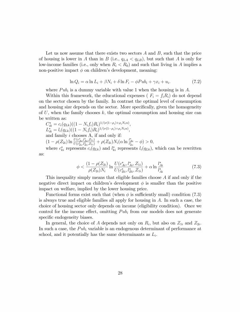


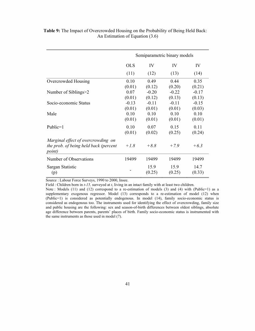


![Photoelectric effect [45 marks] - Peda.net](https://static.documents.pub/doc/80x56/61869499ebec7b11d64c02eb/photoelectric-eect-45-marks-pedanet.jpg)


