1 The Eigen Theory of Waves in Piezoelectric Solids Shaohua Guo Zhejiang University of Science and Technology P.R.China 1. Introduction It is difficult to answer how many elastic waves exist in anisotropic solids. The traditional viewpoint believes that there are only two bulk elastic waves in solids, one is the dilation wave discovered by Poisson in 1892, and the other the shear wave discovered by Stokes in 1899. The existence of the P-wave and the S-wave was also verified by the classical elastic theory. However, with the discovery of some new phenomena of elastic waves in anisotropic solids, it is found that the limitations of classical elastic theory have become obvious. Furthermore, the current concepts and theories of elastic waves can not answer several basic questions of elastic wave propagation in anisotropic solids. For example, how many elastic waves are there? How many wave types are there? What is the space pattern of elastic waves? As we know, the Christoffel’s equation, which is often used to describe anisotropic elastic waves in the classical elastic theory, can not indicate the space pattern and the complete picture of elastic wave propagation in anisotropic solids, but only show the difference of propagation in the different directions along an axis or a section (Vavrycuk, 2005). The reason for this is that the classical elastic wave equations, expressed by displacements can not distinguish the different elastic sub-waves (except for isotropic solids), because the elasticity and anisotropy of solids are synthesized in an elastic matrix. Similarly, for the electromagnetic fields, except for the Helmholtz’s equation of electromagnetic waves in isotropic media, the laws of propagation of electromagnetic waves in anisotropic media are also not clear to us. From the Maxwell’s equation, the explicit equations of electromagnetic waves in anisotropic media could not be obtained because the dielectric permittivity matrix and magnetic permeability matrix were all included in these equations, so that only local behaviour of electromagnetic waves, for example, in a certain plane or along a certain direction, can be studied (Yakhno et al., 2006). The theory of linear piezoelectricity is based on a quasi-static approximation (Tiersten et al., 1962). In this theory, although the mechanical equations are dynamic, the electromagnetic equations are static and the electric field and the magnetic field are not coupled. Therefore it does not describe the wave behaviour of electromagnetic fields. Electromagnetic waves generated by mechanical fields (Mindlin, 1972) need to be studied in the calculation of radiated electromagnetic power from a vibrating piezoelectric device (Lee et al., 1990), and are also relevant in acoustic delay lines (Palfreeman, 1965) and wireless acoustic wave sensors (Sedov et al., 1986), where acoustic waves produce electromagnetic waves or vise versa. When electromagnetic waves are involved, the complete set of Maxwell equation needs to be used, Source: Acoustic Waves, Book edited by: Don W. Dissanayake, ISBN 978-953-307-111-4, pp. 466, September 2010, Sciyo, Croatia, downloaded from SCIYO.COM www.intechopen.com
Transcript
1
The Eigen Theory of Waves in Piezoelectric Solids
Shaohua Guo Zhejiang University of Science and Technology
P.R.China
1. Introduction
It is difficult to answer how many elastic waves exist in anisotropic solids. The traditional viewpoint believes that there are only two bulk elastic waves in solids, one is the dilation wave discovered by Poisson in 1892, and the other the shear wave discovered by Stokes in 1899. The existence of the P-wave and the S-wave was also verified by the classical elastic theory. However, with the discovery of some new phenomena of elastic waves in anisotropic solids, it is found that the limitations of classical elastic theory have become obvious. Furthermore, the current concepts and theories of elastic waves can not answer several basic questions of elastic wave propagation in anisotropic solids. For example, how many elastic waves are there? How many wave types are there? What is the space pattern of elastic waves? As we know, the Christoffel’s equation, which is often used to describe anisotropic elastic waves in the classical elastic theory, can not indicate the space pattern and the complete picture of elastic wave propagation in anisotropic solids, but only show the difference of propagation in the different directions along an axis or a section (Vavrycuk, 2005). The reason for this is that the classical elastic wave equations, expressed by displacements can not distinguish the different elastic sub-waves (except for isotropic solids), because the elasticity and anisotropy of solids are synthesized in an elastic matrix. Similarly, for the electromagnetic fields, except for the Helmholtz’s equation of electromagnetic waves in isotropic media, the laws of propagation of electromagnetic waves in anisotropic media are also not clear to us. From the Maxwell’s equation, the explicit equations of electromagnetic waves in anisotropic media could not be obtained because the dielectric permittivity matrix and magnetic permeability matrix were all included in these equations, so that only local behaviour of electromagnetic waves, for example, in a certain plane or along a certain direction, can be studied (Yakhno et al., 2006). The theory of linear piezoelectricity is based on a quasi-static approximation (Tiersten et al., 1962). In this theory, although the mechanical equations are dynamic, the electromagnetic equations are static and the electric field and the magnetic field are not coupled. Therefore it does not describe the wave behaviour of electromagnetic fields. Electromagnetic waves generated by mechanical fields (Mindlin, 1972) need to be studied in the calculation of radiated electromagnetic power from a vibrating piezoelectric device (Lee et al., 1990), and are also relevant in acoustic delay lines (Palfreeman, 1965) and wireless acoustic wave sensors (Sedov et al., 1986), where acoustic waves produce electromagnetic waves or vise versa. When electromagnetic waves are involved, the complete set of Maxwell equation needs to be used,
Source: Acoustic Waves, Book edited by: Don W. Dissanayake, ISBN 978-953-307-111-4, pp. 466, September 2010, Sciyo, Croatia, downloaded from SCIYO.COM
www.intechopen.com
Acoustic Waves
2
coupled to the mechanical equations of motion. Such a fully dynamic theory is called piezoelectromagnetism by some researchers (Lee, 1991). Piezoelectromagnetic SH waves were studied by Li (Li, 1996) using scalar and vector potentials, which results in a relatively complicated mathematical model of four equations. Two of these equations are coupled, and the other two are one-way coupled. In addition, a gauge condition needs to be imposed. A different formulation was given by Yang and Guo (Yang et al., 2006), which leads to two uncoupled equations. Piezoelectromagnetic SH waves over the surface of a circular cylinder of polarized ceramics were analyzed. Although many works have been done for the piezoelectromagnetic waves in piezoelectric solids, the explicit uncoupled equations of piezoelectromagnetic waves in the anisotropic media could not be obtained because of the limitations of classical theory. In this chapter, the idea of eigen theory presented by author (Guo, 1999; 2000; 2001; 2002; 2005; 2007; 2009; 2009; 2010; 2010; 2010) is used to deal with both the Maxwell’s electromagnetic equation and the Newton’s motion equation. By this method, the classical Maxwell’s equation and Newton’s equation under the geometric presentation can be transformed into the eigen Maxwell’s equation and Newton’s equation under the physical presentation. The former is in the form of vector and the latter is in the form of scalar. As a result, a set of uncoupled modal equations of electromagnetic waves and elastic waves are obtained, each of which shows the existence of electromagnetic and elastic sub-waves, meanwhile the propagation velocity, propagation direction, polarization direction and space pattern of these sub-waves can be completely determined by the modal equations. In section 2, the elastic waves in anisotropic solids were studied under six dimensional eigen spaces. It was found that the equations of elastic waves can be uncoupled into the modal equations, which represent the various types of elastic sub-waves respectively. In section 3, the Maxwell’s equations are studied based on the eigen spaces of the physical presentation, and the modal electromagnetic wave equations in anisotropic media are deduced. In section 4, the quasi-static theory of waves in piezoelectric solids (mechanical equations of motion, coupled to the equations of static electric field, or Maxwell’s equations, coupled to the mechanical equations of equilibrium) are studied based on the eigen spaces of the physical presentation. The complete sets of uncoupled elastic or electromagnetic dynamic equations for piezoelectric solids are deduced. In section 5, the Maxwell’s equations, coupled to the mechanical equations of motion, are studied based on the eigen spaces of the physical presentation. The complete sets of uncoupled fully dynamic equations for piezoelectromagnetic waves in anisotropic media are deduced, in which the equations of electromagnetic waves and elastic ones are both of order 4. The discussions are given in section 6.
2. Elastic waves in anisotropic solids
2.1 Concepts of eigen spaces
The eigen value problem of elastic mechanics can be written as
1,2, ,6i i i iλ= = ACϕ ϕ (1)
where C is a standarded matrix of elastic coefficients, iλ is eigen elasticity, and is
invariables of coordinates, iϕ is the corresponding eigen vector, and satisfies the
orthogonality condition of basic vectors.
Τ=C ΦΛΦ (2)
www.intechopen.com
The Eigen Theory of Waves in Piezoelectric Solids
3
where 1 2 6, , ,λ λ λ= ⎡ ⎤⎣ ⎦AdiagΛ , { }1 2 6, , ,= AΦ ϕ ϕ ϕ is the modal matrix of elastic solids, it is
orthogonal and positive definite one, satisfies T I=Φ Φ . The eigen spaces of anisotropic elastic solids consist of independent eigen vectors, it has the structure as follows
* *1 1[ ] [ ]m mW W W= ⊕ ⊕Aϕ ϕ (3)
where the possible overlapping roots are considered, and ( )6m ≤ is used to represent the
number of independent eigen spaces. Projecting the stress vector σ and strain vector ε on
the eigen spaces, we get
* * * *1 1 m mσ σ= + +Aσ ϕ ϕ (4)
* * * *1 1 m mε ε= + +Aε ϕ ϕ (5)
where *iσ and *
iε are modal stress and modal strain, which are stress and strain under the
eigen spaces respectively, and are different from the traditional ones in the physical meaning.
Eqs.(4) and (5) are also regarded as a result of the sum of finite number of normal modes. The modal stress and modal strain satisfy the normal Hook’s law
* * 1,2, ,i i i i mσ λ ε= = A (6)
2.2 Modal elastic wave equations When neglecting body force, the dynamics equation and displacement equation of elastic solids are the following respectively
ik k iuσ ρ′ = $$ (7)
1
( )2
ij i j j iu uε ′ ′= + (8)
From Eqs.(7) and (8), we can get the following equation
2ik kj jk ki ijσ σ ρε′ ′+ = $$ (9)
Because of the symmetry on ( ),i j in Eq.(9) we can rewrite it in the form of matrix.
It is seen that Δ is a symmetrical differential operator matrix, and 2 /ij ji i jx x∂ = ∂ = ∂ ∂ ∂ ,
2 /tt t tΔ = ∂ ∂ ∂ .
It is proved by author that the elastic dynamics equation (10) under the geometrical spaces of three dimension can be converted into the modal equations under the eigen spaces of six dimension
* * * 1,2, ,i i i tt i i mλ ε ρΔ εΔ = = A (12)
and
Δ* T* * 1,2, ,i i i i mΔ = = Aϕ ϕ (13)
where *Δ i is called as the stress operator. From Eq.(12), we have
* * *2
1Δ , 1,2, ,i i tt ii
ε ε= ∇ = Ai mv
(14)
The calculation shows that the stress operators are the same as Laplace’s operator (either two dimensions or three dimensions) for isotropic solids, and for most of anisotropic solids. In the modal equations of elastic waves, the speeds of propagation of elastic waves are the following
, 1,2, ,iiv i m
λρ= = A (15)
Eqs.(14) and (15) show that the number of elastic waves in anisotropic solids is equal to that of eigen spaces of anisotropic solids, and the speeds of propagation of elastic waves are related to the eigen elasticity of anisotropic solids.
2.3 Elastic waves in isotropic solids
There are two independent eigen spaces in isotropic solids
(1) (5)1 1 2 2 6[ ] [ , , ]W W W= ⊕ Aϕ ϕ ϕ (16)
where
1 2
3
3 2[1,1,1,0,0,0] , [0,1, 1,0,0,0]
3 2
6[2, 1, 1,0,0,0] , ( 4,5,6)
6
T T
Ti i iξ
⎫= = − ⎪⎪⎬⎪= − − = = ⎪⎭
ϕ ϕϕ ϕ
(17)
where iξ is a vector of order 6, in which i th element is 1 and others are 0. The eigen elasticity and eigen operator of isotropic solids are the following
( )1 2
* 2 * 21 2
3 2 , 2 ,
1 1, ,
3 2III III
λ λ μ λ μ ⎫= + = ⎪⎬Δ = ∇ Δ = ∇ ⎪⎭ (18)
www.intechopen.com
The Eigen Theory of Waves in Piezoelectric Solids
5
where λ and μ are Lame constants, 2III∇ is Laplace’s operator of three dimention. Thus, there
exist two independent elastic waves in isotropic solids, which can be described by the
It will be seen as follows that Eqs.(19) and (20) represent the dilation wave and shear wave respectively. Using Eq. (5), the modal strain of order 1 of isotropic solids is
* T*1 1 11 22 33
3( )
3ε ε ε ε= ⋅ = + +ϕ ε (21)
Eq. (21) represents the relative change of the volume of elastic solids. So Eq. (19) shows the motion of pure longitudinal wave. Also from Eq. (5), the modal strain of order 2 of isotropic solids is
* * * *2 2 1 1ε ε= −ϕ ε ϕ (22)
By the orthogonality condition of eigenvectors, we have
* * * T * * 1/22 1 1 1 1
2 2 2 1/21 2 2 3 3 1
[( ) ( )]
1 { [( ) ( ) ( ) ]}
3
ε ε εε ε ε ε ε ε
= − ⋅ −= − + − + −
ε ϕ ε ϕ (23)
Eq. (23) represents the pure shear strain on elastic solids. So Eq. (20) shows the motion of pure transverse wave.
2.4 Elastic waves in anisotropic solids 2.4.1 Cubic solids
There are three independent eigen spaces in a cubic solids
Thus there exist four independent elastic waves in hexagonal solids, which can be described by following equations
* * *( , ) ( , ) 1,2,3 ,4i i i ix t x t iλ ε ρεΔ = =$$ (33)
where
1,2 11 12* 131,2 11 22 33
2 2131,2 11 12 13
[ ( ) ]( ) 2
c cc
cc c c
λε ε ε ελ− −= × + +− − + (34)
www.intechopen.com
The Eigen Theory of Waves in Piezoelectric Solids
7
( )2* 23 11 22 12
1
2ε ε ε ε= − + (35)
* 2 24 32 31
1( )
2ε ε ε= + (36)
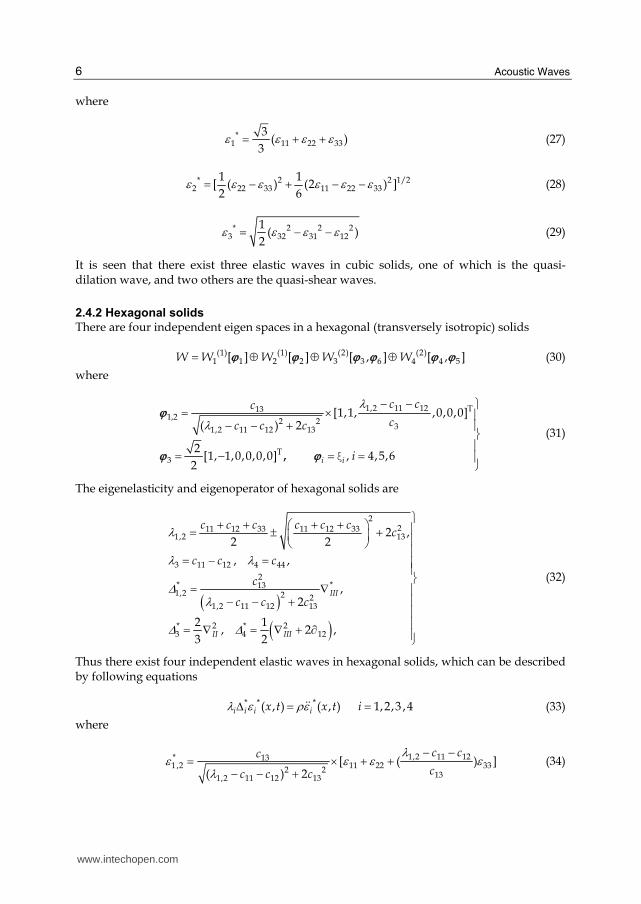
It is seen that there exist four elastic waves in hexagonal solids, two of which are the quasi-dilation wave, and two others are the quasi-shear waves.
3. Electromagnetic waves in anisotropic solids
3.1 Eigen spaces of electromagnetic solids In anisotropic electromagnetic solids, the dielectric permittivity and magnetic permeability are tensors instead of scalars. The constitutive relations are expressed as follows
= ⋅D e E (37)
= ⋅B Hμ (38)
where the dielectric permittivity matrix e and the magnetic permeability matrix μ are
usually symmetric ones, and the elements of the matrixes have a close relationship with the selection of reference coordinate. Suppose that if the reference coordinates is selected along principal axis of electrically or magnetically anisotropic solids, the elements at non-diagonal of these matrixes turn to be zero. Therefore, Eqs. (37),(38) are called the constitutive equations of electromagnetic solids under the geometric presentation. Now we intend to get rid of effects of geometric coordinate on the constitutive equations, and establish a set of coordinate-independent constitutive equations of electromagnetic media under physical presentation. For this purpose, we solve the following problems of eigen-value of matrixes
( ) 0η− =e I φ
(39)
( )γ−μ ϑ = 0I
(40)
where ( )1,2,3I Iη = and ( )1,2,3I Iγ = are respectively eigen dielectric permittivity and
eigen magnetic permeability, which are constants of coordinate-independent. ( )1,2,3I I =φ
and ( )1,2,3I I =ϑ are respectively eigen electric vector and eigen magnetic vector, which
show the electrically principal direction and magnetically principal direction of anisotropic
solids, and are all coordinate-dependent. We call these vectors as eigen spaces. Thus, the
matrix of dielectric permittivity and magnetic permeability can be spectrally decomposed as
follows
=e ΤΨΓΨ (41)
Τ=μ ΘΠΘ (42)
where [ ]1 2 3, ,diag η η η=Γ and [ ]1 2 3, ,diag γ γ γ=Π are the matrix of eigen dielectric
permittivity and eigen magnetic permeability, respectively. { }1 2 3, ,=Ψ φ φ φ and
www.intechopen.com
Acoustic Waves
8
{ }1 2 3, ,=Θ ϑ ϑ ϑ are respectively the modal matrix of electric media and magnetic media,
which are both orthogonal and positive definite matrixes, and satisfy, T = IΨ Ψ , T = IΘ Θ . Projecting the electromagnetic physical qualities of geometric presentation, such as the electric field intensity vector E, magnetic field intensity vector H, magnetic flux density vector B and electric displacement vector D into eigen spaces of physical presentation, we get
Τ= ⋅*
D DΨ Τ= ⋅*
E EΨ (43)
Τ= ⋅*
B BΘ Τ= ⋅*
H HΘ (44) Rewriting Eqs.(43) and (44) in the form of scalar, we have
*I ID Τ= ⋅ I = 1- nDφ
*I IE Τ= ⋅ I = 1- nEφ
(45)
*I IB Τ= ⋅ I = 1 - nBϑ *
I IH Τ= ⋅ I = 1 - nHϑ (46)
where ( )3n ≤ are number of electromagnetic independent subspaces. These are the
electromagnetic physical qualities under the physical presentation. Substituting Eqs. (43) and (44) into Eqs. (37) and (38) respectively, and using Eqs.(45) and (46) yield
* *I I ID Eη= I = 1 - n (47)
* *I I IB Hγ= I = 1 - n (48)
The above equations are just the modal constitutive equations of electromagnetic media in the form of scalar.
3.2 Matrix expression of Maxwell’s equation The classical Maxwell’s equations in passive region can be written as
,IJK K J Ie H D= $ (49)
,IJK K J Ie E B= − $ (50)
Now we rewrite above equations in the form of matrix as follows
In anisotropic dielectrics, the dielectric permittivity is a tensor, while the magnetic permeability is a scalar. So Eqs. (57) and (58) can be written as follows
[ ]{ } [ ]{ }2
0tH e Hμ= −∇M (60)
[ ]{ } [ ]{ }20tE e Eμ= −∇M (61)
Substituting Eqs. (43), (44) and (47) into Eqs. (60) and (61), we have
{ } [ ]{ }* * 2 *0tH Hμ Γ⎡ ⎤ = −∇⎣ ⎦M (62)
{ } [ ]{ }* * 2 *0tE Eμ Γ⎡ ⎤ = −∇⎣ ⎦M (63)
where [ ] [ ][ ]T*⎡ ⎤ = Ψ Ψ⎣ ⎦M M is defined as the eigen matrix of electromagnetic operators under
the eigen spaces, is a diagonal matrix. Thus Eqs. (62) and (63) can be uncoupled in the form
of scalar.
* * 2 *
0 0 1I I I t IH H I nμ η+ ∇ = = −M (64)
www.intechopen.com
Acoustic Waves
10
* * 2 *
0 0 1I I I t IE E I nμ η+ ∇ = = −M (65)
Eqs.(64) and (65) are the modal equations of electromagnetic waves in anisotropic
dielectrics.
3.2.2 Magnetically anisotropic solids
In anisotropic magnetics, the magnetic permeability is a tensor, while the dielectric
permittivity is a scalar. So Eqs. (57) and (58) can be written as follows
[ ]{ } [ ]{ }20tH e Hμ= −∇M (66)
[ ]{ } [ ]{ }20tE e Eμ= −∇M (67)
Substituting Eqs. (43), (44) and (48) into Eqs. (66) and (67), we have
{ } [ ]{ }* * 2 *0tH e HΠ⎡ ⎤ = −∇⎣ ⎦M (68)
{ } [ ]{ }* * 2 *0tE e EΠ⎡ ⎤ = −∇⎣ ⎦M (69)
where [ ] [ ][ ]T*⎡ ⎤ = Θ Θ⎣ ⎦M M is defined as the eigen matrix of electromagnetic operators under
the eigen spaces, is a diagonal matrix. Thus Eqs. (68) and (69)can be uncoupled in the form
of scalar.
* * 2 *0 0 1I I I t IH e H I nγ+ ∇ = = −M (70)
* * 2 *0 0 1I I I t IE e E I nγ+ ∇ = = −M (71)
Eqs.(70) and (71) are the modal equations of electromagnetic waves in anisotropic
magnetics.
3.3 Electromagnetic waves in anisotropic solids
In this section, we discuss the propagation behaviour of electromagnetic waves only in
anisotropic dielectrics.
3.3.1 Isotropic crystal
The matrix of dielectric permittivity of isotropic dielectrics is following
e
e
e
1111
11
0 0⎡ ⎤⎢ ⎥= 0 0⎢ ⎥⎢ ⎥0 0⎣ ⎦e (72)
The eigen-values and eigen-vectors are respectively shown as below
[ ]11 11 11, ,diag e e e=Γ (73)
www.intechopen.com
The Eigen Theory of Waves in Piezoelectric Solids
11
1 0 0
0 1 0
0 0 1
⎡ ⎤⎢ ⎥= ⎢ ⎥⎢ ⎥⎣ ⎦Ψ (74)
We can see from the above equations that there is only one eigen-space in isotropic crystal, which is a triple-degenerate one, and the space structure is following
( ) [ ]3
1 1 2 3, ,W φ φ φ=W (75)
The basic vector of one dimension in a triple-degenerate subspace is
{ }*1
31,1,1
3
T=φ (76)
The eigen-qualities and eigen-operators of isotropic crystal are respectively shown as below
( )*1 1 2 3
1
3E E E E= + + (77)
( )* 2 2 21
1
3x y z
⎡ ⎤= − ∂ + ∂ + ∂⎣ ⎦M (78)
Thus the equations of electromagnetic waves in isotropic crystal can be written as
( )( ) ( )2 2 2 21 2 3 0 11 1 2 3x y z tE E E e E E Eμ∂ + ∂ + ∂ + + = ∂ + + (79)
or
( )2 2 2 21 0 11 1x y z tE e Eμ∂ + ∂ + ∂ = ∂ (80)
( )2 2 2 22 0 11 2x y z tE e Eμ∂ + ∂ + ∂ = ∂ (81)
( )2 2 2 23 0 11 3x y z tE e Eμ∂ + ∂ + ∂ = ∂ (82)
The velocity of the electromagnetic wave is
0 11
1c
eμ= (83)
Eq. (79) is just the Helmholtz’s equation of electromagnetic wave.
3.3.2 Uniaxial crystal
The matrix of dielectric permittivity of uniaxial dielectrics is following
e
e
e
1111
33
0 0⎡ ⎤⎢ ⎥= 0 0⎢ ⎥⎢ ⎥0 0⎣ ⎦e (84)
www.intechopen.com
Acoustic Waves
12
The eigen-values and eigen-vectors are respectively shown as below
[ ]11 11 33, ,diag e e e=Λ (85)
1 0 0
0 1 0
0 0 1
⎡ ⎤⎢ ⎥= ⎢ ⎥⎢ ⎥⎣ ⎦Ψ (86)
We can see from the above equations that there are two eigen-spaces in uniaxial crystal, one of which is a double-degenerate space, and the space structure is following
( ) [ ] [ ]2 1
1 1 2 2 3,W Wφ φ φ= ⊕W (87)
The basic vectors in two subspaces are following
{ }*1
21,1,0
2
T=φ (88)
{ }*2 0,0,1
T=φ (89)
The eigen electric strength qualities of uniaxial crystal are respectively shown as below
T
3
*2 2E = ⋅ EE =φ (90)
T * T *
1 21 2= −E EEφ φ (91)
Multiplying Eq.(91) with 2φ , using T
2 1 0⋅ =φ φ and ( )T 1 1,2i i i⋅ = =φ φ , we get
( ) ( )TT * T *
2 2
* 2 21 2 2 1 2E E E= − − = +E EE Eφ φ (92)
The eigen-operators of uniaxial crystal are respectively shown as below
( )* 2 2 2 21 2 2x y z xy= − ∂ + ∂ + ∂ − ∂M (93)
( )* 2 22 x y= − ∂ + ∂M (94)
Therefore, the equations of electromagnetic waves in uniaxial crystal can be written as below
( )2 2 2 2 2 2 2 2 21 2 0 11 1 22 2x y z xy tE E e E Eμ∂ + ∂ + ∂ − ∂ + = ∂ + (95)
( )2 2 23 0 33 3x y tE e Eμ∂ + ∂ = ∂ (96)
The velocities of electromagnetic waves are respectively as follows
www.intechopen.com
The Eigen Theory of Waves in Piezoelectric Solids
13
( )1
0 11
1c
eμ= (97)
( )2
0 33
1c
eμ= (98)
It is seen that there are two kinds of electromagnetic waves in uniaxial crystal.
3.3.3 Biaxial crystal The matrix of dielectric permittivity of biaxial dielectrics is following
22
33
e
e
e
11 0 0⎡ ⎤⎢ ⎥= 0 0⎢ ⎥⎢ ⎥0 0⎣ ⎦e (99)
The eigen-values and eigen-vectors are respectively shown as below
[ ]11 22 33, ,diag e e e=Λ (100)
1 0 0
0 1 0
0 0 1
⎡ ⎤⎢ ⎥= ⎢ ⎥⎢ ⎥⎣ ⎦Ψ (101)
We can see from the above equations that there are three eigen-spaces in biaxial crystal, and the space structure is following
( ) [ ] ( ) [ ] ( ) [ ]1 1 1
1 1 2 2 3 3W W Wφ φ φ= ⊕ ⊕W (102)
The eigen-qualities and eigen-operators of biaxial crystal are respectively shown as below
T
1
*1 1E = ⋅ EE =φ (103)
T
2
*2 2E = ⋅ EE =φ (104)
T
3
*3 3E = ⋅ EE =φ (105)
( )* 2 21 z y= − ∂ + ∂M (106)
( )* 2 22 x z= − ∂ + ∂M (107)
( )* 2 23 x y= − ∂ + ∂M (108)
Therefore, the equations of electromagnetic waves in biaxial crystal can be written as below
( )2 2 21 0 11 1z y tE e Eμ∂ + ∂ = ∂ (109)
www.intechopen.com
Acoustic Waves
14
( )2 2 22 0 22 2x z tE e Eμ∂ + ∂ = ∂ (110)
( )2 2 23 0 33 3x y tE e Eμ∂ + ∂ = ∂ (111)
The velocities of electromagnetic waves are respectively as follows
( )1
0 11
1c
eμ= (112)
( )2
0 22
1c
eμ= (113)
( )3
0 33
1c
eμ= (114)
It is seen that there are three kinds of electromagnetic waves in biaxial crystal.
3.3.4 Monoclinic crystal
The matrix of dielectric permittivity of monoclinic dielectrics is following
11 12
12 22
33
e e
e e
e
0⎡ ⎤⎢ ⎥= 0⎢ ⎥⎢ ⎥0 0⎣ ⎦e (115)
The eigen-values and eigen-vectors are respectively shown as below
Therefore, the equations of electromagnetic waves in monoclinic crystal can be written as below
( ) ( )1 1
* 21 1 11 12 2 0 1 1 11 12 2te e E e e Eη μ η η⎡ − + ⎤ = ∂ ⎡ − + ⎤⎣ ⎦ ⎣ ⎦M E E (126)
( ) ( )1 1
* 22 12 2 11 2 0 2 12 2 11 2te e E e e Eη μ η η⎡ + − ⎤ = ∂ ⎡ + − ⎤⎣ ⎦ ⎣ ⎦M E E (127)
( )2 2 23 0 33 3x y tE e Eμ∂ + ∂ = ∂ (128)
The velocities of electromagnetic waves are respectively as follows
( )( ) ( )
1
2
211 220 11 22 12
1
1
2 2
c
e ee e eμ
= ⎧ ⎫+⎪ ⎪⎡ ⎤+ − +⎨ ⎬⎢ ⎥⎣ ⎦⎪ ⎪⎩ ⎭
(129)
( )( ) ( )
2
2
211 220 11 22 12
1
1
2 2
c
e ee e eμ
= ⎧ ⎫+⎪ ⎪⎡ ⎤− − +⎨ ⎬⎢ ⎥⎣ ⎦⎪ ⎪⎩ ⎭
(130)
( )3
0 33
1c
eμ= (131)
www.intechopen.com
Acoustic Waves
16
It is seen that there are also three kinds of electromagnetic waves in monoclinic crystal. In
comparison with the waves in biaxial crystal, the electromagnetic waves in monoclinic
crystal have been distorted.
4. Quasi-static waves in piezoelectric solids
4.1 Modal constitutive equation of piezoelectric solids
For a piezoelectric but nonmagnetizable dielectric body, the constitutive equations is the
following
T= ⋅ − ⋅c h Eσ ε (132)
= ⋅ + ⋅D h e Eε (133)
= ⋅B Hμ (134)
where h is the piezoelectric matrix.
Substituting Eqs. (5), (43) and (44) into Eqs. (132)-(134), respectively, and multiplying them
with the transpose of modal matrix in the left, we have
TΤ Τ Τ= −* *c h EΦ σ Φ Φε Φ Ψ (135)
T T T= +* *D h e EΨ Ψ Φε Ψ Ψ (136)
T T *=B HΘ Θ μΘ (137)
Let T=G hΨ Φ , T T T=G hΦ Ψ , that is a coupled piezoelectric matrix, and using Eqs.(2), (41)
and (42), we get
T= −* * *G Eσ Λε (138)
= +* * *D G Eε Γ (139)
* *=B HΠ (140)
Rewriting the above equations in the form of scalar, we have
* * * 1 - 1 -Ti i i iJ Jg E i m J nσ λε= − = = (141)
* * * 1 - 1 -I I I Ij jD E g I n j mη ε= + = = (142)
* * 1 -I I IB H I nγ= = (143)
Eqs.(138)-(140) are just the modal constitutive equations for anisotropic piezoelectric body,
in which { } { }T
Ij I jg hφ ϕ= ⎡ ⎤⎣ ⎦ , { } { }TTTiJ i Jg hϕ φ= ⎡ ⎤⎣ ⎦ , T
iJ Jig g= are the coupled piezoelectric
coefficients.
www.intechopen.com
The Eigen Theory of Waves in Piezoelectric Solids
17
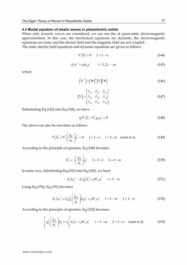
4.2 Modal equation of elastic waves in piezoelectric solids
When only acoustic waves are considered, we can use the of quasi-static electromagnetic approximation. In this case, the mechanical equations are dynamic, the electromagnetic equations are static and the electric field and the magnetic field are not coupled. The static electric field equations and dynamic equations are given as follows
* * 0 1I ID I n∇ = = − (144)
* * * 1,2, ,i i tt i i mσ ρ εΔ = Δ = A (145)
where
[ ] [ ][ ]* T⎡ ⎤∇ = Ψ ∇ Ψ⎣ ⎦ (146)
[ ] 11 21 31
12 22 32
13 23 33
∂ ∂ ∂⎡ ⎤⎢ ⎥∇ = ∂ ∂ ∂⎢ ⎥⎢ ⎥∂ ∂ ∂⎣ ⎦ (147)
Substituting Eq.(142) into Eq.(144), we have
* * * * 0I I I I Ij jE gη ε∇ +∇ = (148)
The above can also be rewritten as follows
* * * * 0 1 - 1 -Ji
J J J i
J
gE J n i mεη
⎛ ⎞∇ +∇ = = =⎜ ⎟⎜ ⎟⎝ ⎠ (sum to i) (149)
According to the principle of operator, Eq.(148) becomes
* * 1 - 1 -Jk
J k
J
gE J n k mεη
⎛ ⎞= − = =⎜ ⎟⎜ ⎟⎝ ⎠ (150)
In same way, Substituting Eq.(141) into Eq.(145), we have
* * * * * 1Ti i i i iJ J tt ig E i mλε ρ εΔ − Δ = ∇ = − (151)
They are the equations of elastic waves in quasi-static piezoelectricity, in which the propagation speed of elastic waves is the folloing
1
JkTi iJ ik
J J
i
gg
v i m
λ δηρ⎛ ⎞+ ⎜ ⎟⎜ ⎟⎝ ⎠= = −
∑ (154)
4.3 Modal equation of electromagnetic waves in piezoelectric solids
When electromagnetic waves are involved, the complete set of Maxwell equation needs to be used, coupled to the static mechanical equations as follows
* * 0 1,2, ,i i i mσΔ = = A (155)
{ } { }* * * * 1I I t I IE B I nϑΔ = −∇ = − (156)
{ } { }* * * * 1I I t I IH D I nφΔ = ∇ = − (157)
Substituting Eq. .(141)-(143) into Eq.(155)-(157), we have
{ } { }* * * 1I I t I I IE H I nϑ γΔ = −∇ = − (158)
{ } { }( )* * * * 1I I t I I I Ij jH E g I nφ η εΔ = ∇ + = − (159)
( )* * * 0 1Ti i i iJ JλεΔ − = = −g E i m (160)
Transposing Eq.(158), and multiplying it with { }*IΔ , and also using Eq.(159), we have
{ }{ } { } { } ( )* * * * *T T
I I I tt I I I I I Ij jE E gϑ φ γ η εΔ Δ = −∇ + (161)
Let { } { }* * *T
I I I= Δ ⋅ ΔL and { } { }T
I I Iξ ϑ φ= , Eq.(159) can be written as
* * * *I I tt I I I I tt I I Ij jE E gξ γ η ξ γ ε+∇ = −∇L (162)
From Eq.(160), Using the principle of operator, and changing the index, we have
* * 1,2, ,6TjK
j K
j
gE jε λ
⎛ ⎞⎜ ⎟= =⎜ ⎟⎝ ⎠ A (sum to K) (163)
Substituting Eq.(163) into Eq.(162), we get the equations of electric fields
* * * 0TjK
I I tt I I I Ij IK I
j
E g Eξ γ η δλ⎡ ⎤⎛ ⎞⎢ ⎥⎜ ⎟+ ∇ + =⎜ ⎟⎢ ⎥⎝ ⎠⎣ ⎦
Lg
(sum to j, K) (164)
www.intechopen.com
The Eigen Theory of Waves in Piezoelectric Solids
19
In same way, we can get the equations of magnetic fields
* * * 0TjK
I I tt I I I Ij IK I
j
H g Hξ γ η δλ⎡ ⎤⎛ ⎞⎢ ⎥⎜ ⎟+ ∇ + =⎜ ⎟⎢ ⎥⎝ ⎠⎣ ⎦
Lg
(sum to j, K) (165)
Eqs.(164) and (165) are just the eigen equations of electromagnetic waves in piezoelectric solids, the speed of electromagnetic waves are the following
2 11I
TjK
I I I Ij IK
j
c I n
gξ γ η δλ= = −⎡ ⎤⎛ ⎞⎢ ⎥+ ⎜ ⎟⎜ ⎟⎢ ⎥⎝ ⎠⎣ ⎦
g (166)
4.4 Eigen properties of polarized ceramics
In this section, we discuss the propagation laws of piezoelectromagnetic waves in an
polarrized ceramics poled in the 3x -direction. The material tensors in Eqs.(132)-(134) are
represented by the following matrices under the compact notation
11 12 13
12 11 13
13 13 13
44
44
66
0 0 0
0 0 0
0 0 0
0 0 0 0 0
0 0 0 0 0
0 0 0 0 0
c c c
c c c
c c c
c
c
c
⎡ ⎤⎢ ⎥⎢ ⎥⎢ ⎥⎢ ⎥⎢ ⎥⎢ ⎥⎢ ⎥⎢ ⎥⎣ ⎦
,
31
31
33
15
15
0 0
0 0
0 0
0 0
0 0
0 0 0
h
h
h
h
h
⎡ ⎤⎢ ⎥⎢ ⎥⎢ ⎥⎢ ⎥⎢ ⎥⎢ ⎥⎢ ⎥⎢ ⎥⎣ ⎦
, 11
11
33
0 0
0 0
0 0
e
e
e
⎡ ⎤⎢ ⎥⎢ ⎥⎢ ⎥⎣ ⎦,
11
11
33
0 0
0 0
0 0
μμ
μ⎡ ⎤⎢ ⎥⎢ ⎥⎢ ⎥⎣ ⎦
(167)
where ( )66 11 12
1
2c c c= − .
There are four independent mechanical eigenspaces as follows
It is seen that the electric subspaces are the same as magnetic ones for polarrized ceramics. Thus, the physical quantities, the coupled coefficients and the corresponding operators of polarrized ceramics are calculated as follows
4.5 Elastic waves in polarized ceramics There are four equations of elastic waves in polarized ceramics, in which the propagation speed of elastic waves is the folloing, respectively
2 11v
λρ= (181)
( ) ( )2 22 21 31 1 33 2 31 2 33
22 11 332
2 2a h b h a h b h
e ev
λρ
+ ++ += (182)
2 11 123
c cv ρ
−= (183)
215
442 114
hc
ev ρ
+= (184)
It is seen that two of elastic waves are the quasi-dilation wave, and two others are the quasi-shear waves, and only two waves were affected by the piezoelectric coefficients, which speeds up the propagation of second and fourth waves.
4.6 Electromagnetic waves in polarized ceramics There are two equations of electromagnetic waves in polarized ceramics, in which the propagation speed of electromagnetic waves is the folloing, respectively
( )21 22 2
1 31 1 33 1511 11
2 44
1
2c
a h b h he
cμ λ
= ⎡ ⎤+⎢ ⎥+ +⎢ ⎥⎣ ⎦ (185)
( )22 22
2 31 2 3322 22
2
1
2c
a h b heμ λ
= ⎡ ⎤+⎢ ⎥+⎢ ⎥⎣ ⎦ (186)
It is seen that two electromagnetic waves are all affected by the piezoelectric coefficients, which slow down the propagation of electromagnetic waves.
5. Fully dynamic waves in piezoelectric solids
When fully dynamic waves are considered, the complete set of Maxwell equation needs to be used, coupled to the mechanical equations of motion as follows
* * * 1,2, ,i i tt i i mσ ρ εΔ = ∇ = A (187)
{ } { }* * * * 1I I t I IE B I nϑΔ = −∇ = − (188)
www.intechopen.com
Acoustic Waves
22
{ } { }* * * * 1I I t I IH D I nφΔ = ∇ = − (189)
Substituting Eqs. (141)-(143) into Eqs. (187)- (189), respectively, we have
( )* * * *i i i tt iλε ρ εΔ − = ∇T
iJ Jg E (sum to J) (190)
{ } { }* * * 1I I t I I IE H I nϑ γΔ = −∇ = − (191)
{ } { }( )* * * * 1I I t I I I Ij jH E g I nφ η εΔ = ∇ + = − (192)
Transposing Eq.(191), and multiplying it with { }*IΔ , and using Eq.(192), we have
( )* * * 1 1I tt I I I I tt I I Ij jE g I n j mξ γ η ξ γ ε+∇ = −∇ = − = −L (sum to j) (193)
where { }{ }* * *T
I I I= Δ ΔL and { } { }* *T
I I Iξ ϑ φ= . Eq.(190) can be written as follows
( )* * * * 1 1j j tt j jλ ρ εΔ − ∇ = Δ = − = −T
jI Ig E I n j m (sum to I) (194)
where ( )*I tt I I Iξ γ η+∇L and ( )*
j j ttλ ρΔ − ∇ are the electromagnetic dynamic operator and
mechanical dynamic operator, respectively. In order to investigate the mutual effects
between mechanical subspaces and electromagnetic subspaces, multiplying Eq.(191) with
the mechanical dynamic operator and Eq.(192) with the electromagnetic dynamic operator,
and substituting Eq. (194) into Eq. (193) and Eq. (193) into Eq. (194), we have
( )( ) ( ) ( )* ** * *j jTj j tt I tt I I I I tt I I Ij j jK KE gλ ρ ξ γ η ξ γΔ − ∇ +∇ = −∇ ΔL g E (sum to K) (195)
( )( ) ( ) ( )( )* ** * *I I
I tt I I I j j tt j j tt Iξ γ η λ ρ ε ξ γ ε+∇ Δ − ∇ = Δ −∇L T
jI I Ik kg g (sum to k) (196)
where ( )* j
IE notes the I th modal electric field induced by j th mechanical subspace, and ( )* I
jε the j th modal strain field induced by I th electromagnetic subspace. Reorganizing
Eqs.(195) and (196), we get
( ) ( ) ( ) ( )* * ** * * * 0j j jT
tttt I I I I tt I j I I j I Ij jK KI I j j I IE g E Eρ ξ γ η ρ ξ γ λη δ λ⎡ ⎤∇ +∇ −Δ + − Δ =⎣ ⎦L Lg
1 1= − = −I n j m (sum to k) (197)
( ) ( ) ( ) ( )* * ** * * * 0I I IT
tttt I I I j tt I j I I j I Ij jK KI j j j I jgρ ξ γ η ε ρ ξ γ λη δ ε λ ε⎡ ⎤∇ +∇ −Δ + − Δ =⎣ ⎦L Lg
1 1= − = −I n j m (sum to k) (198)
In same way, we can obtain the modal magnetic field equations as follows
( ) ( ) ( ) ( )* * ** * * * 0j j j
tttt I I I I tt I j I I j I Ij I j j I Iρ η γ ξ ρ γ ξ λη δ λ⎡ ⎤∇ +∇ −Δ + − Δ =⎣ ⎦L LT
jK KIH g g H H
www.intechopen.com
The Eigen Theory of Waves in Piezoelectric Solids
23
1 1= − = −I n j m (sum to k) (199)
From the above results, we can see that when considering the mutual effects between mechanical subspaces and electromagnetic subspaces, the electromagnetic wave equations become four-order partial differential ones, meanwhile elastic wave equation still keep in the form of four-order partial differential ones.
6. Conclusions
In the first place, we analyzed here the elastic waves and electromagnetic waves in
anisotropic solids. The calculation shows that the propagation of elastic waves in anisotropic
solids consist of the incomplete dilation type and the incomplete shear type except for the
pure longitudinal or pure transverse waves in isotropic solids. Several novel results for
elastic waves were obtained, for example, there are two elastic waves in isotropic solids,
which are the P-wave and the S-wave. There are three elastic waves in cubic solids, one of
which is a quasi-P-waves and two are quasi-S-waves. There are four elastic waves in
hexagonal (transversely isotropic) solids, half of which are quasi-P-waves and half of which
are quasi-S-waves. There are five elastic waves in tetragonal solids, two of which are quasi-
P-waves and three of which are quasi-S-waves. There are no more than six elastic waves in
orthotropic solids or in the more complicated anisotropic solids. For electromagnetic waves,
the similar results were obtained: 1) the number of electromagnetic waves in anisotropic
media is equal to that of eigen-spaces of anisotropic media; 2) the velocity of propagation of
electromagnetic waves is dependent on the eigen-dielectric permittivity and eigen-magnetic
permeability; 3) the direction of propagation of electromagnetic waves is related on the
eigen electromagnetic operator in the corresponding eigen-space; 4) the direction of
polarization of electromagnetic waves is relevant to the eigen-electromagnetic quantities in
the corresponding eigen-space. In another word, there is only one kind of electromagnetic
wave in isotropic crystal. There are two kinds of electromagnetic waves in uniaxial crystal.
There are three kinds of electromagnetic waves in biaxial crystal and three kinds of distorted
electromagnetic waves in monoclinic crystal. Secondly, the elastic waves and
electromagnetic waves in piezoelectric solids both for static theory and for fully dynamic
theory are analyzed here based on the eigen spaces of physical presentation. The results
show that the number and propagation speed of elastic or electromagnetic waves in
anisotropic piezoelectric solids are determined by both the subspaces of electromagnetically
anisotropic media and ones of mechanically anisotropic media. For the piezoelectric
material of class 6mm, it is seen that there exist four elastic waves, respectively, but only two
waves were affected by the piezoelectric coefficients. There exist two electromagnetic waves,
respectively, but the two waves were all affected by the piezoelectric coefficients. The fully
dynamic theory of Maxwell’s equations, coupled to the mechanical equations of motion, are
studied here. The complete set of uncoupled dynamic equations for piezoelectromagnetic
waves in anisotropic media are deduced. For the piezoelectric material of class 6mm, it will
be seen that there exist eight electromagnetic waves and also eight elastic waves,
respectively. Furthermore, in fact of I jc v4 , except for the classical electromagnetic waves
and elastic waves, we can obtain the new electromagnetic waves propagated in speed of
elastic waves and new elastic waves propagated in speed of electromagnetic waves.
www.intechopen.com
Acoustic Waves
24
7. References
Guo, S. H. (1999). Eigen theory of elastic dynamics for anisotropic solids. Trans. Nonferr. Met. Soc. China, 9., 2., 63–74, 1003-6326
Guo, S. H. (2000). Eigen theory of elastic mechanics for anisotropic solids. Trans. Nonferr. Met. Soc. China, 10., 2., 173–184, 1003-6326
Guo, S. H. (2001). Eigen theory of viscoelastic mechanics for anisotropic solids. Acta Mech. Solida Sinica, 22., 4., 368–374, 0894-9166
Guo, S. H. (2002). The standard expression of the engineering mechanical vector and the invariant of elastic mechanics. Acta Mech. Solida Sinica, 15., 1., 74-80, 0254-7805
Guo, S. H. (2005). Eigen theory of viscoelastic dynamics based on the Kelvin-Voigt model. Appl. Math. Mech., 25., 7., 792–798, 0253-4827
Guo, S. H. (2008). An eigen theory of rheology for complex media. Acta Mech., 198., 3/4., 253-260, 0001-5970
Guo, S. H. (2009). An eigen theory of electromagnetic waves based on the standard spaces. Int. J. Engng. Sci., 47., 3., 405-412, 0020-7225
Guo, S. H. (2009). An Eigen theory of Static Electromagnetic Field for Anisotropic Media. Appl. Math. Mech., 30., 5., 528-533, 0253-4827
Guo, S. H. (2010). An eigen theory of waves in piezoelectric solids. Acta Mech. Sinica, 26., 2., 280-288, 0567-7718
Guo, S. H. (2010). An eigen theory of electro-magnetic acoustic waves in magnetoelectroelastic media. Acta Mech., 211., 4., 173-180, 0001-5970
Guo, S. H. (2010). An eigen expression for piezoelectrically stiffened elastic and dielectric constants based on the static theory. Acta Mech., 210., 3., 345-350, 0001-5970
Lee, P. C. Y.; Kim, Y. G.& Prevost, J. H. (1990). Electromagnetic radiation from doubly rotated piezoelectric crystal plates vibrating at thickness frequencies. J. Appl. Phys., 67., 6633-6642, 0021-8979
Lee, P. C. Y. (1991). A variational principle for the equations of piezoelectromagnetism in elastic dielectric crystals. J. Appl. Phys., 69., 7470-7473, 0021-8979
Li, S. (1996). The electromagneto-acoustic surface wave in a piezoelectric medium: the Bleustein-Gulyaev mode. J. Appl. Phys., 80., 5264-5269, 0021-8979
Mindlin, R. D. (1973). Electromagnetic radiation from a vibrating quartz plate. Int. J. Solids Struct., 9., 6., 697-702, 0020-7683
Palfreeman, J. S.(1965). Acoustic delay lines-A survey of types and uses. Ultrasonics, 3., 1., 1-8, 0041-624x
Sedov, A.; Schmerr, Jr.; et al. (1986). Some exact solutions for the propagation of transient electroacoustic waves I: piezoelectric half-space. Int. J. Engng. Sci., 24., 4., 557-568, 0020-7225
Tiersten, H. F.; Mindlin, R. D. (1962). Forced vibrations of piezoelectric crystal plates. Quart. Appl. Mech., 20., 2., 107-119, 0033-569x
Vavrycuk, V. (2005). Acoustic axes in weak triclinic anisotropy. Geophysical Journal International, 163., 2., 629-638, 0956-540x
Yakhno, V. G.; Yakhno, T. M. & Kasap, M. (2006). A novel approach for modeling and simulation of electromagnetic waves in anisotropic dielectrics. Int. J. Solids Struct., 43., 20., 6261-6276, 0020-7683
Yang, J.S.; Guo, S. H. (2006). Piezoelectromagnetic waves guided by the surface of a ceramic cylinder. Acta Mech., 181., 3/4., 199-205, 0001-5970
www.intechopen.com
Acoustic WavesEdited by Don Dissanayake
ISBN 978-953-307-111-4Hard cover, 434 pagesPublisher SciyoPublished online 28, September, 2010Published in print edition September, 2010
InTech ChinaUnit 405, Office Block, Hotel Equatorial Shanghai No.65, Yan An Road (West), Shanghai, 200040, China
Phone: +86-21-62489820 Fax: +86-21-62489821
SAW devices are widely used in multitude of device concepts mainly in MEMS and communication electronics.As such, SAW based micro sensors, actuators and communication electronic devices are well knownapplications of SAW technology. For example, SAW based passive micro sensors are capable of measuringphysical properties such as temperature, pressure, variation in chemical properties, and SAW basedcommunication devices perform a range of signal processing functions, such as delay lines, filters, resonators,pulse compressors, and convolvers. In recent decades, SAW based low-powered actuators and microfluidicdevices have significantly added a new dimension to SAW technology. This book consists of 20 excitingchapters composed by researchers and engineers active in the field of SAW technology, biomedical and otherrelated engineering disciplines. The topics range from basic SAW theory, materials and phenomena toadvanced applications such as sensors actuators, and communication systems. As such, in addition totheoretical analysis and numerical modelling such as Finite Element Modelling (FEM) and Finite DifferenceMethods (FDM) of SAW devices, SAW based actuators and micro motors, and SAW based micro sensors aresome of the exciting applications presented in this book. This collection of up-to-date information and researchoutcomes on SAW technology will be of great interest, not only to all those working in SAW based technology,but also to many more who stand to benefit from an insight into the rich opportunities that this technology hasto offer, especially to develop advanced, low-powered biomedical implants and passive communicationdevices.
How to referenceIn order to correctly reference this scholarly work, feel free to copy and paste the following:
Shaohua Guo (2010). The Eigen Theory of Waves in Piezoelectric Solids, Acoustic Waves, Don Dissanayake(Ed.), ISBN: 978-953-307-111-4, InTech, Available from: http://www.intechopen.com/books/acoustic-waves/the-eigen-theory-of-waves-in-piezoelectric-solids