Abstract The paper studies how high-income taxpayers responded to the introductionof the “extraordinary tax on individuals” in Hungary in 2007. The study is based on apanel of tax returns containing information on 10 % of tax filers from 2005 and threesubsequent years. We estimate the elasticity of taxable income with respect to themarginal net-of-tax rate and find that the taxable income of Hungarian high earners ismoderately responsive to taxation: the estimated elasticity is about 0.24. We also findevidence for a sizeable income effect. The estimated effect is not caused by incomeshifting.
Keywords Taxable income elasticity · Personal income tax · Tax avoidance ·Income shifting · Income effect
JEL Classification H20 · H24 · H31 · J22
1 Introduction
The elasticity of taxable income with respect to the marginal tax rate is a parameterof great policy relevance. Having a reliable estimate of the elasticity enables the
Á. Kiss (B)National Bank of Hungary (MNB), Szabadság tér 8-9, Budapest 1054, Hungarye-mail: [email protected]
P. MosbergerCentral European University, Nádor utca 9, Budapest 1051, Hungarye-mail: [email protected]
Present addressÁ. KissEuropean Commission, Directorate General for Economic and Financial Affairs, Brussels, Belgium
123
Á. Kiss, P. Mosberger
policy-makers to make more accurate fiscal assessments of changes to the tax system.The elasticity also enables researchers to quantify the dead-weight loss of incometaxation.1
The importance of the taxable income elasticity is reflected in the growing literatureof empirical work. The first estimates of taxable income elasticity based on a panelof tax returns were conducted by Feldstein (1995). The method used by Feldsteinidentifies two similar groups of taxpayers whose tax rates are affected differentlyby a change in tax rules. If the growth of reported taxable income differs betweenboth groups, then it is most likely caused by the change of tax rates. Later analysesdeveloped regression methodologies that are able to control for many confoundingfactors in large panels (see, e.g., Auten and Carroll 1999; Gruber and Saez 2002).Recent surveys of the literature are provided by Giertz (2004) and Saez et al. (2012).
While the literature focused on the U.S. at the beginning, more recently empiricalwork was done on other countries as well, such as Canada (Sillamaa and Veall 2001;Saez and Veall 2005), Norway (Aarbu and Thoresen 2001), Sweden (Ljunge andRagan 2004; Hansson 2007; Holmlund and Söderström 2007; Blomquist and Selin2010), Hungary (Bakos et al. 2008),2 Germany (Gottfried and Witczak 2009), Finland(Pirttilä and Selin 2011), and Denmark (Kleven and Schultz 2011).
While the empirical literature is growing, many important questions about the back-ground of the estimated elasticities remain open. One important question is to whatextent the estimated elasticities reflect labor supply response on the intensive margin(whether that is hours worked, work intensity, or occupation choice) and to what extentthey reflect income-shifting or changing tax-avoidance behavior.
The present paper studies how high-income taxpayers in Hungary responded to theintroduction of the “extraordinary tax on individuals” in January 2007. The extraordi-nary tax was a 4 % surcharge on income above the pension contribution ceiling. Theanalysis is based on a panel of tax returns, compiled by the National Tax Authority forthis study, containing anonymous information on 10 % of tax filers in 2005 and threeconsecutive years.
In our main specification, the elasticity of taxable income with respect to the mar-ginal net-of-tax rate is estimated to be 0.24. This estimate is somewhat lower thanmost estimates for the U.S., but similar to many estimates for other countries. (Manyestimates outside the U.S. are below 0.4, the preferred elasticity of Gruber and Saez(2002), which is itself in the lower range of U.S. estimates.) We also find evidence fora sizeable income effect.
Besides offering an analysis of a new policy episode outside the U.S., the paperintends to contribute to the literature in three ways. First, it focuses on a clean policyepisode that affected high earners. As in other countries, high-income earners have agreat economic and fiscal significance in Hungary. In 2008, the lower income limit ofthe extraordinary tax was HUF 7.1 million (about EUR 28,000 at the contemporary
1 The relationship between the elasticity of the taxable income and the dead-weight loss of taxation wasanalyzed by Feldstein (1999) and Chetty (2009).2 Updated results of Bakos et al. (2008) have been described by Benczúr et al. (2013) for a non-technicalaudience.
123
The elasticity of taxable income of high earners
exchange rate). The tax thus affected the top 2.5 % of tax filers who controlled 16 %of the aggregate tax base and paid 28 % of total personal income tax.3
Second, the focus on a well-defined group of high-income earners, and the relativelylarge number of observations, makes it possible for us to address a methodologicalproblem many studies struggle with. It is known since the early literature that gen-eral income growth may differ across various segments of the income distribution forreasons not related to the change in the tax rates. On the one hand, incomes at thetop might disproportionally grow because of skill-biased technological change. Onthe other hand, the phenomenon of “regression to the mean” might affect individualswith very high or very low incomes at a given point in time. Since Auten and Carroll(1999) and Gruber and Saez (2002), it is a common practice to address this problem bycontrolling for initial income. Still, results are often sensitive to the way initial incomeis controlled for, especially in studies where a broad income range is analyzed or thevery top of the income distribution is involved. This study focuses on a relatively nar-row range around the income limit at which the extraordinary tax was introduced. Ourresults are not sensitive to whether initial income is controlled for, which indicates thatthe sample that we concentrate on is homogeneous enough. The phenomena of mean-reversion or differential income trends do not affect parts of our sample differently.
Third, we are able to conduct indirect tests suggesting that the estimated elasticitydoes not reflect income shifting.4 First, we do not find differential growth of capitalincome for taxpayers who are likely, prior to the tax change, to be affected by theextraordinary tax. Second, high-income taxpayers with wage income only, presumablythe least able to engage in income shifting, exhibit a similar elasticity of taxable incomeas individuals who have other incomes as well. This may indicate that most of the effectis caused by the adjustment of labor supply (whether it be hours or work intensity), butother explanations (such as the change in tax evasion, adjustment through non-wagebenefits, etc.) cannot be excluded.
The rest of the paper is organized as follows. Section 2 describes the theoreticalbackground, the Hungarian personal income tax system, the data, and the empiricalspecification. Section 3 presents the results of the main specification and provides somerobustness checks and indirect evidence about the causes of the estimated elasticity.A discussion of the results concludes.
2 Methodology and data
2.1 Theoretical background and problems of identification
Estimations of the elasticity of taxable income with respect to the tax rates are moti-vated by a simple theoretical framework in which the labor supply decision of an opti-
3 Own calculation based on a 10 % random sample of 2008 tax returns, excluding the full-time self-employed.4 In contrast, Goolsbee (2000) finds evidence in the US that a substantial part of the response of high-income individuals to tax changes is of a short-term nature, involving the timing of certain transactions,and thus does not represent real labor supply adjustment.
123
Á. Kiss, P. Mosberger
mizing individual is modeled (see Appendix B for details).5 Taxes affect the trade-offbetween leisure and consumption. The following relationship between income growthand tax rates can be derived from optimization:
� log y = β� log (1 − METR) + φ� log(1 − AETR), (1)
where y is a taxable income, METR is the marginal effective tax rate, and AETR is theaverage effective tax rate. (We call them effective tax rates because social security con-tributions on the employee’s side are also taken into account.) The variable (1−METR)is the marginal net-of-tax rate. It measures what share of additional taxable incomethe taxpayer can keep. This is the central variable of the taxable income literature. Thecoefficient of this variable β measures to what extent taxpayers respond to marginalincentives or, in other words, to what extent they generate less taxable income whenfacing a higher marginal tax rate.
The variable (1−AETR) is the average net-of-tax rate. It measures what share oftotal taxable income the taxpayer can keep as net income. The coefficient of thisvariable φ measures the income effect: the extent to which taxpayers generate lesstaxable income if they receive a lump-sum transfer (or tax relief). If two taxpayershave the same taxable income and the same marginal tax rate, but face a differentaverage tax rate, then this means that the tax system treats them differently by a lump-sum component.6
The researcher faces two problems when estimating the relationship between tax-able income and the tax rates. The first problem is that the income distribution mightchange for reasons independent of the tax changes: for instance, wage dispersion mightincrease because of skill-biased technological change. Another problem, having theopposite effect, is the phenomenon of “regression to the mean”: some individuals ofextraordinarily high incomes might be experiencing a lucky year, most likely to befollowed by a decrease in income. These phenomena might bias the estimation bymaking high incomes appear to grow faster or slower following a change in the taxcode. The literature, following Auten and Carroll (1999), deals with this problem byincluding (log) initial income (i.e., taxable income in the period before the tax change)as a control variable. The coefficient of initial income will be negative if the phenom-enon of regression to the mean is significant or if the income distribution becomesmore compressed for reasons independent of the tax changes, while it will be positiveif the income distribution becomes more dispersed for independent reasons. Includinginitial income as well as demographic variables to control for individual heterogeneityof taxable income growth, we arrive to the following equation:
� log yi = x ′iα + γ y0i + β� log (1 − METRi ) + φ� log (1 − AETRi ) + ui , (2)
where vector x ′ includes demographic control variables and y0 is initial income.
5 The approach taken here follows Feldstein (1999), Gruber and Saez (2002), and Bakos et al. (2008).6 Previous studies chose different ways to operationalize the income effect in the empirical specification.This formulation follows Bakos et al. (2008) whose operationalization is a slight variant of that of Gruber andSaez (2002). For the derivation of this form and its comparison to Gruber and Saez (2002), see Appendix B.
123
The elasticity of taxable income of high earners
The second econometric problem to be taken care of is that there is inverse causal-ity between the dependent variable and some explanatory variables. Taxable incomemight change for many other reasons independent of taxation. If taxable income of anindividual grows above average, then this will, in a progressive tax system, increasetheir tax rate. A simple OLS regression might, spuriously, indicate that a tax hikemakes taxable income grow faster.
This problem is solved here, as in much of the literature, using the instrumentalvariable (IV) estimation procedure. The instruments for the actual (endogenous) taxrates are the so-called “synthetic tax rates.” These are obtained by applying the after-change tax rules to the (indexed) before-change taxable income of each individual.Since they are based on before-change individual information only, they are exogenousto the after-change income. The details of the procedure as applied in this analysis aredescribed after the description of the data.
2.2 The Hungarian personal income tax (PIT) system during the period of study
The basic principles of the Hungarian PIT system have been fairly stable since thetransition. It is an individual (as opposed to family based) tax system. Total annualincome of an individual is divided into two parts: taxable income7 and capital income.8
During the period, taxable income was subject to a (progressive) piecewise-linear taxfunction, while capital income was taxed at flat tax rates (which depended on the typeof capital income but not on the tax base) that were lower than the upper income taxrate.
The progressive tax schedule that applied to taxable income consisted of two maintax brackets. The lower tax rate was 18 % during the period. The upper tax rate was38 % in 2005 and 36 % in 2008. The threshold between both tax brackets was raisedfrom HUF 1.5 million (about EUR 6,000) to 1.7 million. The change that motivatesour study is the introduction of the “extraordinary tax of individuals” in 2007.9 Thiswas a 4 percentage point surtax applying to income above HUF 7,139,000 (about EUR28,500) in 2008, effectively creating a third tax bracket for high-income earners. (Themain parameters of PIT are summarized in the top panel of Table 1).
Since we are interested in taxpayers’ reaction to the tax rates applying to “taxableincome,” it is natural that we focus on this definition of income in this study. (InSect. 3.3.2 we investigate how capital income of high earners changed between 2005and 2008.)
Taxable income included three main types of income: (1) wage income (includingcost reimbursements, severance pay, and some social benefits); (2) entrepreneurialincome (including income from contract work and income of licensed small-scale
7 The official Hungarian term is, in literal translation, “aggregated tax base” (“összevont adóalap”).8 The official Hungarian term is, in literal translation, “separately taxed incomes” (“külön adózójövedelmek”).9 The extraordinary tax of individuals was introduced by Act 59 of 2006 of the Republic of Hungary.According to paragraph 8, the extraordinary tax, as applied to those individuals who are not full-time self-employed, came into effect on January 1, 2007. The official Hungarian name of the tax is “magánszemélyekkülönadója.”
123
Á. Kiss, P. Mosberger
Table 1 Tax and contribution rates of Hungarian high-income earners in 2005 and 2008
2005 (%) 2008 (%)
Personal income tax (PIT)
PIT lower rate 18 18
Upper limit of lower tax bracket HUF 1.5 M HUF 1.7 M
PIT upper rate 38 36
Extraordinary tax on individuals (surtax on upper rate) – 4
Lower income threshold of extraordinary tax – HUF 7.139 M
Social Security Contributions (SSC)
Employee pension contribution rate 8.5 9.5
Pension contribution ceiling HUF 6.0 M HUF 7.139 M
Other employee contributions 5 7.5
Marginal effective tax rates (METR)
Typical METR at income HUF 5 million 51.5 53
Typical METR at income HUF 8 million 43 47.5
Typical (1-METR) at income HUF 5 million 48.5 47
Percentage change relative to 2005 – −3.09
Typical (1-METR) at income HUF 8 million 57 52.5
Percentage change relative to 2005 – −7.89
Source: Hungarian Tax Authority and own calculations
agricultural producers); and (3) “other taxable income” (income from scholarships inhigher education, some social benefits and, under some circumstances, income earnedabroad). This third group of income was special because although it was part of thetax base, it was not taxed itself.10 Although no taxes were paid after these incomes,they could push other incomes into the higher tax bracket. Pensions, untaxed until2006, became “other taxable income” in 2007, which meant, in effect, that individualswhose only income was from pensions continued to pay no income tax, but the wageincome of pension recipients came to be taxed at a higher rate than before.
The PIT system included a number of tax credits. All tax credits diminished thetaxes payable after a given tax base, rather than diminishing the tax base itself.11 By farthe largest tax credit was the employee tax credit (ETC),12 a non-refundable tax crediton earned income for low- and middle-income individuals with a gradual withdrawalphase at intermediate income levels. Individuals in our sample were not eligible forthe ETC in 2005 since they earned high income. However, we took into account theETC to the extent that it affected actual 2008 taxes of individuals whose income fellto relatively low levels.
10 This is why the official Hungarian term for this group of incomes is “income not bearing tax burden”(“adóterhet nem viselo járandóság”).11 For this reason, there is not as great a difference between ’taxable income’ and ’gross income’ inHungary as in the US.12 The Hungarian term is ’adójóváírás.’
123
The elasticity of taxable income of high earners
The child tax credit (CTC)13 diminished the tax payable by an amount that dependedon the number of dependent children. Married or cohabiting couples could decidewhich one of them claimed the CTC. Couples could also divide the amount of creditbetween them. The CTC became less generous during the period of our study. Tax-payers with one or two children were not eligible any more for the credit in 2008, butthe amount of credit for taxpayers with three or more children was reduced as well. Inboth years, the CTC was withdrawn at a rate of 20 % at relatively high income levels.The withdrawal phase started at income level HUF 8 million in 2005; in 2008, thewithdrawal threshold varied between HUF 6 and 8 million depending on the numberof children.14
Finally, a number of tax credits (including that for charitable giving) were subjectto a common cap of HUF 100,000 (about EUR 400). This set of tax credits was alsowithdrawn at a rate of 20 % starting at a total income of HUF 6 million in 2005 andHUF 3.4 million in 2008.
Income in Hungary is not only subject to PIT but also to social security contributions(SSC), which finance the pension, healthcare, and unemployment benefit systems. SSCare paid by both employees and employers. Similar to Bakos et al. (2008), we takeinto account the effect of employee contributions on average and marginal effectivetax rates, since they drive a wedge between gross and net income the same wayas the PIT does.15 This is justified if the link between contributions and benefits isnot closely linked (at least in the expectations of taxpayers). Benefits do not dependon contributions in healthcare (except for sick leave payments and some pecuniarychild care benefits), but there is a link in the case of pensions. However, we believethat the perceived link between contributions and benefits is weak for three reasons.First, the marginal conversion rate from pension contributions to future benefits isnot transparent in the Hungarian system. Second, changes to the pension system arefrequent and significant. Finally, further changes can be expected since the long-termsustainability of the pension system is in question. Therefore, we believe that we arejustified to assume that employee SSC are perceived the same way as taxes.
The rates of employee SSC in 2005 and 2008 are summarized in the middle panelof Table 1. Employee contribution rates increased from a total of 13.5–17 % in threeyears. Employee pension contributions are subject to a cap. The “pension contributionceiling” was at a high income level, and it is the income level at which the extraordinarytax was introduced.
The bottom panel of Table 1 calculates the METR (and its inverse) for typicaltaxpayers at annual income levels of HUF 5 million and 8 million in 2005 and 2008.It shows that, as a result of all changes, the METR of typical taxpayers earning HUF8 million increased by 4.5 % points, almost exactly by the rate of the extraordinarytax. The METR of high-income individuals below the pension contribution ceiling,not affected by the extraordinary tax, increased by 1.5 % points.
13 The Hungarian term is ’családi adókedvezmény.’14 Note that the withdrawal of all tax credits was conditional on “total income,” that is, the sum of taxableincome and capital income.15 Employer contributions were paid at a rate of 32 % both in 2005 and in 2008.
123
Á. Kiss, P. Mosberger
2.3 Data and sample
The data base was compiled by the Hungarian tax authority for the purposes of thisstudy. It contains information about a panel of anonymous individual tax returns fromthe years 2005 through 2008, based on a 10 % random sample of the population oftax filers in 2005, excluding the full-time self-employed. Not all taxpayers filed a taxreturn in all four years: while we observe 422,219 individuals in 2005, only 359,409of these filed a tax return in 2008. Attrition is less severe among high-income earnerswho are the subject of this study: there are 14,467 taxpayers in the sample of 2005with taxable income above HUF 5 million (about EUR 20,000).16 Of these, 13,237filed a tax return, and 13,159 had non-zero taxable income, in 2008.
The estimation is based on comparing the taxable income growth of different indi-viduals between 2005 and 2008. The “natural experiment” this paper uses for identi-fication includes all tax changes that affected high-income individuals between bothyears. By far the most important of the changes was the introduction of the extraordi-nary tax on individuals effective from January 2007. This episode would theoreticallyallow 2006 to be chosen as base year. However, 2006 is not suitable as a base yearbecause some changes in taxes and contributions, passed together with the extraordi-nary tax, took effect already in September 2006. Thus, in some cases, it is not clearwhat the relevant effective tax rate is for a given individual, and behavior in 2006 mayalready reflect a response to some of the policy changes. Therefore, 2005 was chosenas the base year. As comparison year, 2008 was chosen because changes in taxpayerbehavior might take time. It is for this reason that most studies in the literature considerthe effect of tax changes on a three-year horizon (see, e.g., Feldstein 1995; Gruber andSaez 2002). As a robustness check, results for the period 2005–2007 are also reported.
The potential estimation bias, discussed in Sect. 2.1, caused by “regression to themean” or secular trends in inequality is remedied in two different ways in this paper.The first of these ways, based on the procedure of Auten and Carroll (1999) and thelater literature, is to include (log) initial income as a control variable in the estimatedregressions. The other way to deal with these issues is to focus on a subsample that isas homogeneous as possible so that the disturbing factors not to affect the lower andthe upper end of the sample very differently. The main results presented in this paperare based on a sample that includes individuals having taxable income between HUF5 and 8 million in 2005 (about EUR 20–32 thousand).17 The robustness of the resultsto the sample’s income limits is examined in Sect. 3.2.
To be able to compare the income of individuals between the years 2005 and 2008,we have to take into account the changes to the legal definition of taxable incomeduring these years. As described in the previous subsection, pension income becamepart of the tax base in 2007. Since the effects of this measure should not contaminatethe results, and since we do not observe pension income in 2005, all individuals with
16 During the period 2005–2008, the exchange rate varied around the convenient equivalence EUR 1 =HUF 250. We use this exchange rate to interpret figures in Hungarian Forints (HUF) in the text.17 While this income range, evaluated at the current exchange rate, would be considered a middle-incomesample in the economy of a highly developed country, it is within the top 5 percent of income earners inHungary.
123
The elasticity of taxable income of high earners
pension income in 2008 were left out of the sample. Of the 8,588 taxpayers in thesample with taxable income between HUF 5 and 8 million in 2005, 1,363 had to beexcluded for this reason. After removing these individuals from the sample, we have7,225 observations.
We also exclude 314 taxpayers that either have “other taxable income,” or incomefrom abroad.18 We can assume that the behavior of individuals with income fromabroad does not reflect typical reactions to Hungarian tax rates. For a minority ofthese individuals “other taxable income” comes from child care benefit of parents withchildren under age 3 (“gyes”) or child care benefit of parents with three dependentchildren of whom the youngest is between 3 and 8 years old (“gyet”); since bothbenefits were conditional on the recipient not working full-time outside their homes, weexclude these taxpayers from the sample. Since their number is small, results are robustto their exclusion. Finally, we exclude 16 observations for which information aboutthe residence cannot be observed.19 We thus have 6,895 observations in our sample.
2.4 Variables and descriptive analysis
Individual characteristics like gender, age, and the type of locality of residence(Budapest, large cities, other cities, and villages) are used to generate control variablesin the regressions. Regional controls are not included since they were not significantin any specification. It should be noted that information about the taxpayer’s gender isnot part of a tax file as prepared by the taxpayer. The tax authority has run an algorithmbased on first names to generate this information. As this procedure is imperfect, itmay not be able to identify the gender in case of uncommon, misspelled, or foreignnames. Therefore, gender information is missing for 537 observations in our mainsample. We tagged these observations with a dummy variable and included them inthe analysis.20
In addition, we generate two control variables based on the information of 2005 taxreturns. The first one is a dummy variable that takes the value of 1 if a taxpayer hadhigh capital income in 2005 (defined as more than HUF 150 thousand, or about 600Euro). The other is a dummy variable that takes the value of 1 if the taxpayer chosetax filing through his or her employer in 2005. This option meant that a taxpayer’semployer prepared and sent one’s tax file to the tax authority, saving considerabletime and energy for the employer. A taxpayer had this option if he or she did not haveoutside incomes. The variable thus differentiates between taxpayers who had a singlesource of employment income in 2005 from those who had more sources of income(including contract work, second job, etc.). Both groups may differ in their ability toavoid taxes, but possibly also in other ways.
18 For the majority of high-income individuals earning, “other taxable income,” it is income from abroad.Income earned abroad can, however, also be reported in another line of the tax file, depending on the type ofincome and the source country where it was earned. In an earlier version of this paper (Kiss and Mosberger2011), we failed to exclude 5 individuals with income from abroad.19 For another 21 observations, the locality could be identified despite an erroneous (outdated) postal code.20 The results are robust to their exlusion. In an earlier version of this paper (Kiss and Mosberger 2011),we estimated the elasticity separately for men and women; results were similar to the overall results.
123
Á. Kiss, P. Mosberger
Marginal net-of-tax rates (1 − METR) and average net-of-tax rates (1 − AETR)are calculated based on tax rules described in Sect. 2.2. The bottom panel of Table 1shows the “typical” METR at the top and the bottom of our sample.
Regressions in this paper are estimated with the instrumental variable (IV) proce-dure to deal with the endogeneity of the marginal and average net-of-tax rate. Theinstruments are the “synthetic” counterparts of these. They are obtained by applyingthe 2008 tax rules to inflated 2005 taxable income. The index used to inflate 2005incomes is the average income growth of the sample. (Taxable income grew, on aver-age, by 16.6 %. Results are not sensitive to the precise index of nominal incomegrowth.)
In the first stage of the IV estimation, the actual 2008 marginal and average net-of-tax rates are regressed on all control variables included in the main regression and thecorresponding “synthetic” tax rates. The predicted 2008 tax rates obtained from thefirst-stage regressions are not endogenous any more to 2008 income; therefore, theycan be used to explain 2008 income in the second stage.
Table 2 shows the descriptive statistics of the benchmark sample. Women constituteslightly less than one-third of the sample. Information on gender is missing for about8 % of the sample. More than one-third of the sample live in Budapest (the populationof Budapest, the capital city, is less than one-fifth of Hungary’s population), one-fourthlive in large cities, and another one-fourth in other cities, while 15 % live in villages.About 6 % of our high-income sample had high capital income in 2005, while 44 %chose tax filing through their employer.
Taxable income of individuals in the sample grew by an average of 16.6 % in threeyears; some individuals had near-zero taxable income in 2008, while some saw theirtaxable income multiply by a factor of six. The last four lines of Table 2 summarizethe actual and synthetic tax rates. The statistics show that tax rates (average as wellas marginal) rose in the course of three years. The variation is, naturally, higher inthe change of individuals’ actual tax rates than in the change of their synthetic taxrates.
Figure 1 summarizes information regarding the tax rates and income change in themain sample. The four panels show, respectively, the 2005 marginal and average taxrates, the expected change of the marginal tax rate (where the expected 2008 marginalrate is the synthetic marginal tax rate), and the percentage change in income.
The upper left panel shows the actual 2005 marginal effective tax rate (METR) asa function of 2005 taxable income. Most high-income taxpayers form two continuouslines in the bottom part of the panel: their METR corresponds to the regular tax andcontribution rates below and above the pension contribution ceiling. Their METR is51.5 and 43 %, respectively (see Table 1 for details). Atypical values for the METRare only observed for those who fall into the withdrawal phase of a tax credit. Most ofthese taxpayers have taxable income between HUF 6 and 6.5 million (about EUR 24–26 thousand). They are eligible for one of the tax credits whose common withdrawalphase is in exactly that income range. However, since the withdrawal is based on totalincome (the sum of taxable income and capital income), some taxpayers fall into thiswithdrawal phase with a taxable income below HUF 6 million. They are the scattereddots to the left of the HUF 6 million mark in the top left part of the panel. Atypicaltaxpayers to the right of the HUF 6.5 million mark are those who are in the withdrawal
123
The elasticity of taxable income of high earners
Table 2 Descriptive statistics of the sample
Variable Mean SD Min Max
Female 0.311 0 1
Gender info missing 0.078 0 1
Birth year 1964 1940 1986
Residence: Budapest 0.360 0 1
Residence: large city 0.244 0 1
Residence: other city 0.249 0 1
Residence: village 0.147 0 1
High capital income in 2005 0.059 0 1
Tax filing through employer 0.440 0 1
Taxable income 2005, HUF thousand 6149.6 835.1 5000.0 7999.4
Taxable income 2008, HUF thousand 7167.4 3001.2 2.8 43362
Change of taxable income, 2005–2008 0.166 0.460 −1.000 6.412
Change of actual (1 − METR) −0.019 0.147 −0.526 0.842
Change of synthetic (1 − METR) −0.035 0.126 −0.443 0.649
Change of actual (1 − AETR) −0.027 0.097 −0.206 0.551
Change of synthetic (1 − AETR) −0.060 0.019 −0.400 −0.037
Note The sample consists of 6,895 taxpayers with 2005 taxable income between HUF 5–8 million. In thelast five rows, a value of 0 means no change; −0.5 means a 50 % reduction; 1 means a growth of 100 %.
phase of the child tax credit (and reach the withdrawal threshold of HUF 8 million intotal income because of their capital income).
The lower left panel in Fig. 1 shows the percentage change (as opposed to thechange in percentage points) from the actual 2005 METR to the synthetic 2008 METR.The figure shows that all typical taxpayers see their METR increase somewhat from2005 to 2008: this is the result of the general increase in SSC. Taxpayers above thepension contribution ceiling face the extraordinary tax in addition: an increase in theirMETR of about 4 % points or about 10 %. Just above the 2005 contribution ceiling,there is a short interval of taxable income where individuals face a 20 % increasein their METR. They are taxpayers who are above the contribution ceiling in 2005but are expected to fall under the increased contribution ceiling by 2008 (the ceilingwas raised in discretionary moves by the legislature at a higher rate than incomesgrew in the sample). Other atypical taxpayers see their METR increase or decreasesubstantially because of the changes in the withdrawal phases of tax credits.
The upper right panel in Fig. 1 shows the actual 2005 average effective tax rate(AETR) as a function of 2005 tax base. Most taxpayers are close to the average taxrates that track the statutory rates with only tax credits differentiating between them.Finally, the bottom right panel shows the change of taxable income in the main sample.Clearly, there is great variation in the income growth around its mean: some taxpayerssee that their taxable income reduced to almost zero, while others see their taxableincome multiply. The regression analysis below investigates whether income growthhas a systematic relationship with marginal and effective tax rates.
123
Á. Kiss, P. Mosberger
Fig. 1 Tax rates and change in taxable income, 2005–2008
3 Estimation results
3.1 Results from the main specification
Every regression below is estimated with the IV procedure that can be thought of asa two-stage procedure. In the first step, the actual 2008 marginal net-of-tax-rate isregressed on its synthetic counterpart and the control variables of the main regression.(If the average net-of-tax rate is included as an explanatory variable it also has a first-stage regression. In that case, both synthetic tax rates are included in both first-stageregressions.) The synthetic marginal net-of-tax rate is a good instrument: its coefficientin the first-stage regression for its realized counterpart is about 0.7 (not reported inthe results) and significant on all conventional levels of significance. Initial income,synthetic average net-of-tax rate and most of the demographic control variables arealso statistically significant in the first-stage regression, while the R2 is around 0.45.
More systematic diagnostic tests are reported in the regression tables below. In anIV estimation, the researcher generally faces two problems: one is whether the instru-ments are exogenous, while the other is whether they are relevant. The exogeneityof the instruments is ensured by the way we constructed them based on informationprior to the tax changes. As to the problem of relevance, we report the p-value of theKleibergen–Paap underidentification test (the generalization of the Anderson canon-ical correlations test for the case of non-i.i.d. errors). Under the null hypothesis, theequation is underidentified. Also, we report the partial F-statistics for the first-stageregressions. Since the problem of “weak identification” is known to make estimatorsperform poorly even in cases when the underidentification test is rejected, we also
123
The elasticity of taxable income of high earners
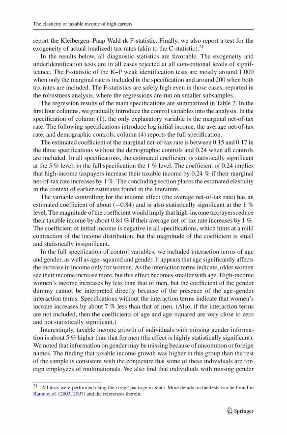
report the Kleibergen–Paap Wald rk F-statistic. Finally, we also report a test for theexogeneity of actual (realized) tax rates (akin to the C-statistic).21
In the results below, all diagnostic statistics are favorable. The exogeneity andunderidentification tests are in all cases rejected at all conventional levels of signif-icance. The F-statistic of the K–P weak identification tests are mostly around 1,000when only the marginal rate is included in the specification and around 200 when bothtax rates are included. The F-statistics are safely high even in those cases, reported inthe robustness analysis, where the regressions are run on smaller subsamples.
The regression results of the main specifications are summarized in Table 2. In thefirst four columns, we gradually introduce the control variables into the analysis. In thespecification of column (1), the only explanatory variable is the marginal net-of-taxrate. The following specifications introduce log initial income, the average net-of-taxrate, and demographic controls; column (4) reports the full specification.
The estimated coefficient of the marginal net-of-tax rate is between 0.15 and 0.17 inthe three specifications without the demographic controls and 0.24 when all controlsare included. In all specifications, the estimated coefficient is statistically significantat the 5 % level; in the full specification the 1 % level. The coefficient of 0.24 impliesthat high-income taxpayers increase their taxable income by 0.24 % if their marginalnet-of-tax rate increases by 1 %. The concluding section places the estimated elasticityin the context of earlier estimates found in the literature.
The variable controlling for the income effect (the average net-of-tax rate) has anestimated coefficient of about (−0.84) and is also statistically significant at the 1 %level. The magnitude of the coefficient would imply that high-income taxpayers reducetheir taxable income by about 0.84 % if their average net-of-tax rate increases by 1 %.The coefficient of initial income is negative in all specifications, which hints at a mildcontraction of the income distribution, but the magnitude of the coefficient is smalland statistically insignificant.
In the full specification of control variables, we included interaction terms of ageand gender, as well as age–squared and gender. It appears that age significantly affectsthe increase in income only for women. As the interaction terms indicate, older womensee their income increase more, but this effect becomes smaller with age. High-incomewomen’s income increases by less than that of men, but the coefficient of the genderdummy cannot be interpreted directly because of the presence of the age–genderinteraction terms. Specifications without the interaction terms indicate that women’sincome increases by about 7 % less than that of men. (Also, if the interaction termsare not included, then the coefficients of age and age–squared are very close to zeroand not statistically significant.)
Interestingly, taxable income growth of individuals with missing gender informa-tion is about 5 % higher than that for men (the effect is highly statistically significant).We noted that information on gender may be missing because of uncommon or foreignnames. The finding that taxable income growth was higher in this group than the restof the sample is consistent with the conjecture that some of these individuals are for-eign employees of multinationals. We also find that individuals with missing gender
21 All tests were performed using the ivreg2 package in Stata. More details on the tests can be found inBaum et al. (2003, 2007) and the references therein.
123
Á. Kiss, P. Mosberger
information are younger, on average, than the rest of the sample (65 % is younger than35 as opposed to 37 % of the whole high-income sample) and is more concentratedin Budapest than the rest (46 % lives in the capital as opposed to about 36 % of thewhole high-income sample).
The type of locality is controlled for by dummy variables; the comparison groupis Budapest. The results show that in the course of three years, income growth in thesample was about 3 % points higher in large cities than in Budapest; while it wasabout 3 % points lower in villages than in Budapest. Only the first of these effects arestatistically significant at the 10 % level.
Of the tax-related control variables, only the dummy for employer filing is sta-tistically significant. The estimated coefficient suggests that the taxable income oftaxpayers choosing this option grew by an additional 5 % as compared to others.This could be a reflection of the notion that individuals with a stable and high-payingemployment contract see their income fall less often than individuals whose highincome comes from multiple sources. The other tax-related control variable, the pres-ence of high capital income, does not appear to affect the growth of taxable incomesignificantly. The estimated coefficient is positive. If shifting earned income to capitalincome played an important role in the reaction to a tax increase on earned income,then we should expect the opposite. (Sect. 3.3.2 provides some direct evidence aboutthe absence of income shifting.)
3.2 Robustness analysis
Two robustness checks are reported in this subsection. The first robustness checklooks at whether results are sensitive to the income limits of the sample. In the secondrobustness check, the main analysis is repeated for the time period 2005–2007 (asopposed to 2005–2008).
3.2.1 Robustness to sample limits
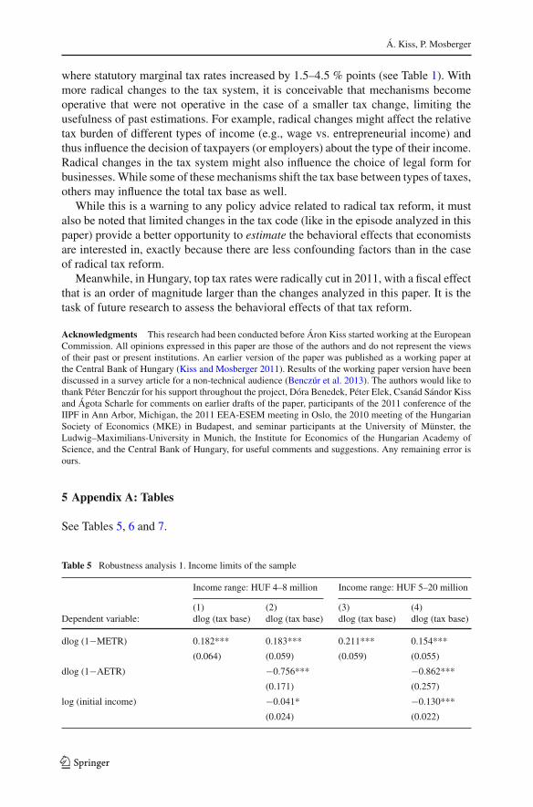
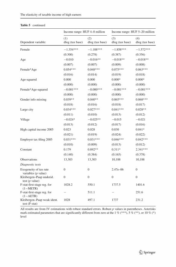
The first robustness check looks at whether results change if the sample is not restrictedto taxpayers with a tax base of HUF 5–8 million in 2005. We broadened the sampleboth upward and downward. The results are reported in Table 5 in Appendix. The fullspecifications are reported in columns (2) and (4). The regressions reported in columns(1) and (3) exclude initial income and the average net-of-tax rate.
The first two columns of the table report results based on a sample of individualsearning HUF 4–8 million in 2005. The estimated coefficients are very similar to thoseobtained with the baseline sample. The coefficient of the marginal net-of-tax rate isslightly lower, about 0.18, still statistically significant at the 1 % level. As a differencefrom the baseline results is that the coefficient of initial income is somewhat higher inabsolute value (about −0.04) and statistically significant at the 10 % level. Comparingcolumns (1) and (2), it appears that results are not sensitive to the inclusion of initialincome and the average net-of-tax-rate.
The last two columns of Table 5 report results based on a sample including taxpayerswith income between HUF 5–20 million in 2005. The results are again qualitatively
123
The elasticity of taxable income of high earners
similar to the main results. In column (3), where only the demographic controls areincluded, the main elasticity is about 0.21 and statistically significant on the 1 %level. Including initial income and the average net-of-tax rate as control variables incolumn (4) makes the elasticity fall to a level of about 0.15, maintaining its statisticalsignificance.
In this specification, including higher incomes as well, the estimated coefficient ofinitial income is large in absolute value (−0.13), and is now statistically significant atthe 1 % level. The economic interpretation of this coefficient is that, all other thingsequal, 1 % higher taxable income in 2005 implies that a taxpayer’s income is expectedto grow by about 0.13 % less. The difference between the estimated coefficient of themarginal net-of-tax rate in column (3) and (4) suggests that, in this broader sample,the inclusion of initial income interferes with the identification of the substitutioneffect. This is a potential problem noted by past literature [notably by Gruber andSaez (2002)]. We conclude that our choice of a more restricted income range for ourbaseline sample is justified: the sample remains more homogeneous, and controllingfor initial income does not interfere with the identification of the tax rate variables.Nevertheless, we note that our main results are qualitatively robust to modificationsof the income limits of the sample.
3.2.2 Robustness to the time period
In the second robustness check, the growth of taxable income is analyzed during theperiod 2005–2007 (rather than 2005–2008, as in the main analysis). The year 2007 wasthe first year after the introduction of the extraordinary tax. Thus, these results show theimmediate effect of the tax changes, while the main specification measures the effectin the second year after the tax changes. (The tax system remained virtually unchangedfrom 2007 to 2008). Results are shown in Table 6 in Appendix. The columns (1)–(4)report results of specifications where control variables are gradually added, similarlyto Table 3.
The results are qualitatively similar to the main results. The estimated coefficientof the marginal net-of tax rate is between 0.10 and 0.13 before controls are added, andabout 0.2 after controls are added. The estimated coefficient is statistically significantat the 1 % level in the full specification and at least at the 10 % level in all otherspecifications. The result suggests that taxpayers’ response became stronger in thecourse of time.
Demographic control variables have a broadly similar effect than in the baselinesample. The interaction of age–squared and gender was not statistically significant andwas, therefore, excluded. This affects the coefficient of the age–gender interaction, butthe result remains that women’s income growth is lower, the disadvantage becomingsmaller with age.
3.3 What lies behind the elasticity?
Perhaps the most intriguing question related to the taxable income elasticity is howmuch of it reflects adjustments in labor supply (reflected either in hours worked or work
123
Á. Kiss, P. Mosberger
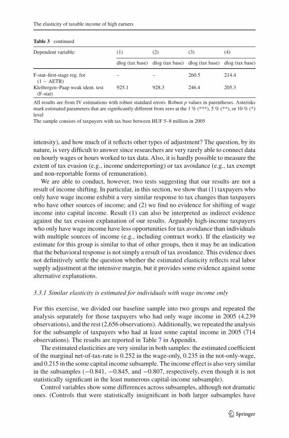
Table 3 Regression results in the main specifications
All results are from IV estimations with robust standard errors. Robust p values in parentheses. Asterisksmark estimated parameters that are significantly different from zero at the 1 % (***), 5 % (**), or 10 % (*)levelThe sample consists of taxpayers with tax base between HUF 5–8 million in 2005
intensity), and how much of it reflects other types of adjustment? The question, by itsnature, is very difficult to answer since researchers are very rarely able to connect dataon hourly wages or hours worked to tax data. Also, it is hardly possible to measure theextent of tax evasion (e.g., income underreporting) or tax avoidance (e.g., tax exemptand non-reportable forms of remuneration).
We are able to conduct, however, two tests suggesting that our results are not aresult of income shifting. In particular, in this section, we show that (1) taxpayers whoonly have wage income exhibit a very similar response to tax changes than taxpayerswho have other sources of income; and (2) we find no evidence for shifting of wageincome into capital income. Result (1) can also be interpreted as indirect evidenceagainst the tax evasion explanation of our results. Arguably high-income taxpayerswho only have wage income have less opportunities for tax avoidance than individualswith multiple sources of income (e.g., including contract work). If the elasticity weestimate for this group is similar to that of other groups, then it may be an indicationthat the behavioral response is not simply a result of tax avoidance. This evidence doesnot definitively settle the question whether the estimated elasticity reflects real laborsupply adjustment at the intensive margin, but it provides some evidence against somealternative explanations.
3.3.1 Similar elasticity is estimated for individuals with wage income only
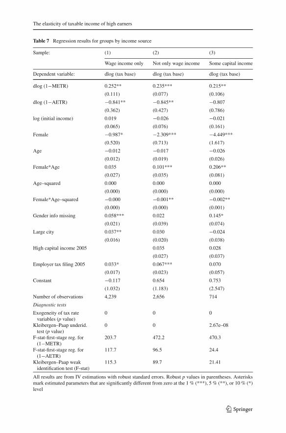
For this exercise, we divided our baseline sample into two groups and repeated theanalysis separately for those taxpayers who had only wage income in 2005 (4,239observations), and the rest (2,656 observations). Additionally, we repeated the analysisfor the subsample of taxpayers who had at least some capital income in 2005 (714observations). The results are reported in Table 7 in Appendix.
The estimated elasticities are very similar in both samples: the estimated coefficientof the marginal net-of-tax-rate is 0.252 in the wage-only, 0.235 in the not-only-wage,and 0.215 in the some capital income subsample. The income effect is also very similarin the subsamples (−0.841, −0.845, and −0.807, respectively, even though it is notstatistically significant in the least numerous capital-income subsample).
Control variables show some differences across subsamples, although not dramaticones. (Controls that were statistically insignificant in both larger subsamples have
123
Á. Kiss, P. Mosberger
been dropped.) The sign of the coefficient of initial income is different in the wage-only and not-only-wage subsamples, but the magnitude is small in both cases and isstatistically insignificant. The interaction of gender and age seems to be significant onlyin the not-only-wage subsample; here, we get the pattern seen in the baseline results,while the interaction terms are insignificant in the wage-only subsample. Missinggender information, on the other hand, is smaller and insignificant in the not-only-wage sample.
3.3.2 No evidence for income shifting (capital income shows no differential response)
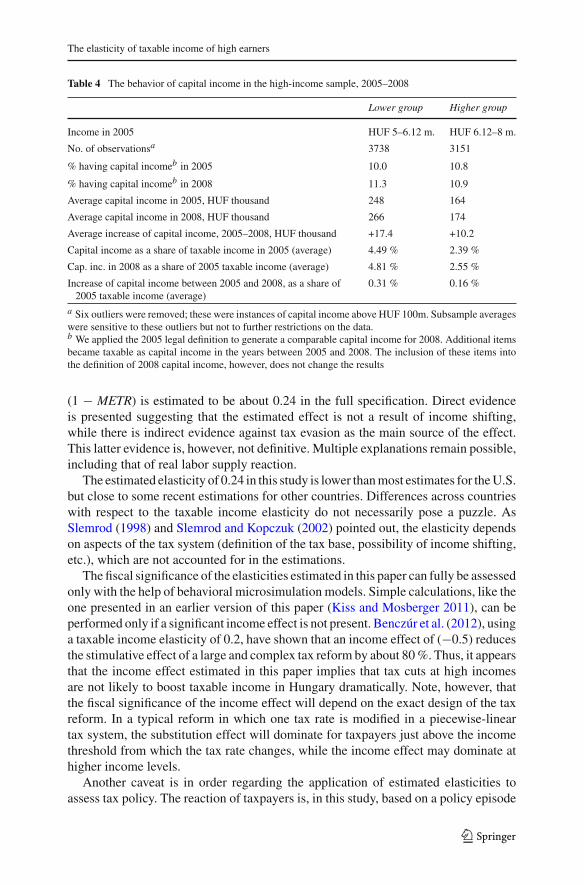
If tax shifting explained much of the elasticity estimated in this paper, then we shouldobserve a differential increase in capital income of those individuals who are likely,ex-ante, to become subject to the extraordinary tax. In this spirit, we divided ourbaseline sample into two subgroups: individuals who, based on the average growthrate of income, are expected to be subject to the extraordinary tax in 2008 (the “higher-income group”), and those who are not (“lower-income group”).
Since three new types of capital income were defined between 2005 and 2008, weapplied the 2005 definition also in 2008 to keep the two years comparable. The newtypes of income are not very significant: combined, they represented about 3 % ofcapital income in our high-income sample. It is thus not surprising that, repeating thesame exercise with contemporaneous definitions of capital income, we get the sameresults.
The lower income group consists of 3,738 taxpayers, while there are 3,151 taxpayersin the higher income group. Six outliers were excluded from the sample: these werecases where an individual received capital income of HUF 100 million (about EUR400,000) or higher. The income earned by these six individuals was great enough tomove the results; the results are robust to any further restriction on the sample. Thesummary statistics of this comparison are shown in Table 4.
Contrary to what could be expected based on the income-shifting explanation, thereis no indication in the data that the higher income group increased its capital incometo a greater extent than the lower income group. Indeed, the share of taxpayers whohave reported positive capital income grew more in the lower income group (a growthof 1.3 % points compared to 0.1). Average capital income stayed largely flat in bothgroups, increasing by a mere HUF 17,000 (EUR 68) for the lower income group asopposed to HUF 10,000 (EUR 36) for the higher income group. The results stay thesame if we compare capital income of both groups as a share of 2005 tax base or as ashare of contemporaneous tax base.
In sum, there is no indication that capital income increased more for the groupaffected by the extraordinary tax.
4 Discussion
The paper examines how high-income taxpayers in Hungary responded to the intro-duction, in 2007, of the extraordinary tax on individuals and other tax changes. Theelasticity of high earners’ taxable income with respect to the marginal net-of-tax rate
123
The elasticity of taxable income of high earners
Table 4 The behavior of capital income in the high-income sample, 2005–2008
Lower group Higher group
Income in 2005 HUF 5–6.12 m. HUF 6.12–8 m.
No. of observationsa 3738 3151
% having capital incomeb in 2005 10.0 10.8
% having capital incomeb in 2008 11.3 10.9
Average capital income in 2005, HUF thousand 248 164
Average capital income in 2008, HUF thousand 266 174
Average increase of capital income, 2005–2008, HUF thousand +17.4 +10.2
Capital income as a share of taxable income in 2005 (average) 4.49 % 2.39 %
Cap. inc. in 2008 as a share of 2005 taxable income (average) 4.81 % 2.55 %
Increase of capital income between 2005 and 2008, as a share of2005 taxable income (average)
0.31 % 0.16 %
a Six outliers were removed; these were instances of capital income above HUF 100m. Subsample averageswere sensitive to these outliers but not to further restrictions on the data.b We applied the 2005 legal definition to generate a comparable capital income for 2008. Additional itemsbecame taxable as capital income in the years between 2005 and 2008. The inclusion of these items intothe definition of 2008 capital income, however, does not change the results
(1 − METR) is estimated to be about 0.24 in the full specification. Direct evidenceis presented suggesting that the estimated effect is not a result of income shifting,while there is indirect evidence against tax evasion as the main source of the effect.This latter evidence is, however, not definitive. Multiple explanations remain possible,including that of real labor supply reaction.
The estimated elasticity of 0.24 in this study is lower than most estimates for the U.S.but close to some recent estimations for other countries. Differences across countrieswith respect to the taxable income elasticity do not necessarily pose a puzzle. AsSlemrod (1998) and Slemrod and Kopczuk (2002) pointed out, the elasticity dependson aspects of the tax system (definition of the tax base, possibility of income shifting,etc.), which are not accounted for in the estimations.
The fiscal significance of the elasticities estimated in this paper can fully be assessedonly with the help of behavioral microsimulation models. Simple calculations, like theone presented in an earlier version of this paper (Kiss and Mosberger 2011), can beperformed only if a significant income effect is not present. Benczúr et al. (2012), usinga taxable income elasticity of 0.2, have shown that an income effect of (−0.5) reducesthe stimulative effect of a large and complex tax reform by about 80 %. Thus, it appearsthat the income effect estimated in this paper implies that tax cuts at high incomesare not likely to boost taxable income in Hungary dramatically. Note, however, thatthe fiscal significance of the income effect will depend on the exact design of the taxreform. In a typical reform in which one tax rate is modified in a piecewise-lineartax system, the substitution effect will dominate for taxpayers just above the incomethreshold from which the tax rate changes, while the income effect may dominate athigher income levels.
Another caveat is in order regarding the application of estimated elasticities toassess tax policy. The reaction of taxpayers is, in this study, based on a policy episode
123
Á. Kiss, P. Mosberger
where statutory marginal tax rates increased by 1.5–4.5 % points (see Table 1). Withmore radical changes to the tax system, it is conceivable that mechanisms becomeoperative that were not operative in the case of a smaller tax change, limiting theusefulness of past estimations. For example, radical changes might affect the relativetax burden of different types of income (e.g., wage vs. entrepreneurial income) andthus influence the decision of taxpayers (or employers) about the type of their income.Radical changes in the tax system might also influence the choice of legal form forbusinesses. While some of these mechanisms shift the tax base between types of taxes,others may influence the total tax base as well.
While this is a warning to any policy advice related to radical tax reform, it mustalso be noted that limited changes in the tax code (like in the episode analyzed in thispaper) provide a better opportunity to estimate the behavioral effects that economistsare interested in, exactly because there are less confounding factors than in the caseof radical tax reform.
Meanwhile, in Hungary, top tax rates were radically cut in 2011, with a fiscal effectthat is an order of magnitude larger than the changes analyzed in this paper. It is thetask of future research to assess the behavioral effects of that tax reform.
Acknowledgments This research had been conducted before Áron Kiss started working at the EuropeanCommission. All opinions expressed in this paper are those of the authors and do not represent the viewsof their past or present institutions. An earlier version of the paper was published as a working paper atthe Central Bank of Hungary (Kiss and Mosberger 2011). Results of the working paper version have beendiscussed in a survey article for a non-technical audience (Benczúr et al. 2013). The authors would like tothank Péter Benczúr for his support throughout the project, Dóra Benedek, Péter Elek, Csanád Sándor Kissand Ágota Scharle for comments on earlier drafts of the paper, participants of the 2011 conference of theIIPF in Ann Arbor, Michigan, the 2011 EEA-ESEM meeting in Oslo, the 2010 meeting of the HungarianSociety of Economics (MKE) in Budapest, and seminar participants at the University of Münster, theLudwig–Maximilians-University in Munich, the Institute for Economics of the Hungarian Academy ofScience, and the Central Bank of Hungary, for useful comments and suggestions. Any remaining error isours.
5 Appendix A: Tables
See Tables 5, 6 and 7.
Table 5 Robustness analysis 1. Income limits of the sample
Income range: HUF 4–8 million Income range: HUF 5–20 million
All results are from IV estimations with robust standard errors. Robust p values in parentheses. Asterisksmark estimated parameters that are significantly different from zero at the 1 % (***), 5 % (**), or 10 % (*)level
123
Á. Kiss, P. Mosberger
Table 6 Robustness analysis 2. Time period 2005–2007
All results are from IV estimations with robust standard errors. Robust p values in parentheses. Asterisksmark estimated parameters that are significantly different from zero at the 1 % (***), 5 % (**), or 10 % (*)level
123
The elasticity of taxable income of high earners
Table 7 Regression results for groups by income source
Sample: (1) (2) (3)
Wage income only Not only wage income Some capital income
All results are from IV estimations with robust standard errors. Robust p values in parentheses. Asterisksmark estimated parameters that are significantly different from zero at the 1 % (***), 5 % (**), or 10 % (*)level
123
Á. Kiss, P. Mosberger
6 Appendix B: The derivation of the income effect
In the main specifications we followed Bakos et al. (2008) in the operationalization ofthe income effect. Their solution is a slight variant of that by Gruber and Saez (2002),the difference being a minor step of approximation. In explaining the difference wesomewhat extend the exposition of Bakos et al. (2008).
The starting point of the theory is an optimizing agent who has an income supplyfunction y = y((1 − τ), R), where τ is the marginal tax rate and R is virtual income.Virtual income is defined, in a non-linear tax schedule, by the expression y − T (y) =R + (1 − τ) y, where T (y) is the total tax due at income level y. The agent’s responseto a tax change can be written as:
dy = − ∂y
∂(1 − τ)dτ + ∂y
∂ R∂ R.
Introducing the uncompensated tax price elasticity βu = [(1−τ)/y][∂y/∂(1−τ)],the income effect φ = (1 − τ) ∂y/∂ R and the compensated tax price elasticity β =βu − φ we obtain:
dy
y= −β
dτ
1 − τ+ φ
dR − ydτ
y (1 − τ).
Most studies estimate this equation in a log-log specification, replacing dy/yby log(y2/y1) and (−dτ/(1 − τ)) by log[(1 − τ2) /(1 − τ1)]. Before Gruber andSaez (2002) the income effect was mostly assumed to be zero. They, in contrast,did include the income effect in the estimation by approximating the last term(dR − ydτ)/ (y (1 − τ)) with log[(y2 − T2 (y2)) /(y1 − T1 (y1))]. As they note ina footnote on page 10 they use the approximation y (1 − τ) ≈ y − T (y) to obtain thisform. We can thus reconstruct their derivation as follows:
dR − ydτ
y (1 − τ)≈ d[y − T (y)]
y (1 − τ)≈ d[y − T (y)]
y − T (y)≈ log
[y2 − T2 (y2)
y1 − T1 (y1)
].
The first equation uses the fact that dR − ydτ is equal to the change in tax liabilitywith changing tax rates and a constant income y; the second step makes the approx-imation in the denominator described above; while the last step is just a logarithmicapproximation. Thus the income effect, equal in its original form to the change inafter-tax income divided by after-tax income minus virtual income, is approximatedby the percentage change in after-tax income.
Bakos et al. (2008) use the same approximation y (1 − τ) ≈ y − T (y) to justify adifferent estimated equation. They reach the following income effect:
dR − ydτ
y (1 − τ)≈ log
[(y2 − T2 (y2)) /y2
(y1 − T1 (y1)) /y1
]= dlog (1 − AETR) .
123
The elasticity of taxable income of high earners
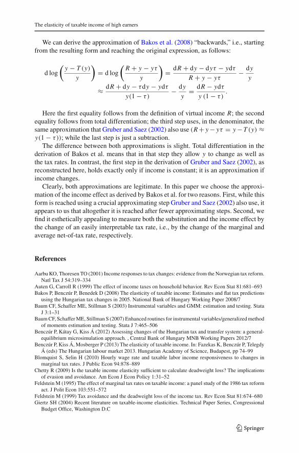
We can derive the approximation of Bakos et al. (2008) “backwards,” i.e., startingfrom the resulting form and reaching the original expression, as follows:
d log
(y − T (y)
y
)= d log
(R + y − yτ
y
)= dR + dy − dyτ − ydτ
R + y − yτ− dy
y
≈ dR + dy − τdy − ydτ
y(1 − τ)− dy
y= dR − ydτ
y (1 − τ).
Here the first equality follows from the definition of virtual income R; the secondequality follows from total differentiation; the third step uses, in the denominator, thesame approximation that Gruber and Saez (2002) also use (R + y − yτ = y − T (y) ≈y(1 − τ)); while the last step is just a subtraction.
The difference between both approximations is slight. Total differentiation in thederivation of Bakos et al. means that in that step they allow y to change as well asthe tax rates. In contrast, the first step in the derivation of Gruber and Saez (2002), asreconstructed here, holds exactly only if income is constant; it is an approximation ifincome changes.
Clearly, both approximations are legitimate. In this paper we choose the approxi-mation of the income effect as derived by Bakos et al. for two reasons. First, while thisform is reached using a crucial approximating step Gruber and Saez (2002) also use, itappears to us that altogether it is reached after fewer approximating steps. Second, wefind it esthetically appealing to measure both the substitution and the income effect bythe change of an easily interpretable tax rate, i.e., by the change of the marginal andaverage net-of-tax rate, respectively.
References
Aarbu KO, Thoresen TO (2001) Income responses to tax changes: evidence from the Norwegian tax reform.Natl Tax J 54:319–334
Auten G, Carroll R (1999) The effect of income taxes on household behavior. Rev Econ Stat 81:681–693Bakos P, Benczúr P, Benedek D (2008) The elasticity of taxable income: Estimates and flat tax predictions
using the Hungarian tax changes in 2005. National Bank of Hungary Working Paper 2008/7Baum CF, Schaffer ME, Stillman S (2003) Instrumental variables and GMM: estimation and testing. Stata
J 3:1–31Baum CF, Schaffer ME, Stillman S (2007) Enhanced routines for instrumental variables/generalized method
of moments estimation and testing. Stata J 7:465–506Benczúr P, Kátay G, Kiss Á (2012) Assessing changes of the Hungarian tax and transfer system: a general-
equilibrium microsimulation approach. , Central Bank of Hungary MNB Working Papers 2012/7Benczúr P, Kiss Á, Mosberger P (2013) The elasticity of taxable income. In: Fazekas K, Benczúr P, Telegdy
Á (eds) The Hungarian labour market 2013. Hungarian Academy of Science, Budapest, pp 74–99Blomquist S, Selin H (2010) Hourly wage rate and taxable labor income responsiveness to changes in
marginal tax rates. J Public Econ 94:878–889Chetty R (2009) Is the taxable income elasticity sufficient to calculate deadweight loss? The implications
of evasion and avoidance. Am Econ J Econ Policy 1:31–52Feldstein M (1995) The effect of marginal tax rates on taxable income: a panel study of the 1986 tax reform
act. J Polit Econ 103:551–572Feldstein M (1999) Tax avoidance and the deadweight loss of the income tax. Rev Econ Stat 81:674–680Giertz SH (2004) Recent literature on taxable-income elasticities. Technical Paper Series, Congressional
Budget Office, Washington D.C
123
Á. Kiss, P. Mosberger
Gottfried P, Witczak D (2009) The responses of taxable income induced by tax cuts: empirical evidencefrom the German taxpayer panel. IAW Discussion Papers No. 57
Goolsbee A (2000) What happens when you tax the rich? Evidence from executive compensation. J PolitEcon 108:352–378
Gruber J, Saez E (2002) The elasticity of taxable income: evidence and implications. J Public Econ 84:1–32Hansson A (2007) Taxpayers’ responsiveness to tax rate changes and implications for the cost of taxation
in Sweden. Int Tax Public Finan 14:563–582Holmlund B, Söderström M (2007) Estimating income responses to tax changes: a dynamic panel data
approach. CESifo Working Paper No. 2121Kiss Á, Mosberger P (2011) The elasticity of taxable income of high earners: evidence from Hungary.
Central Bank of Hungary MNB Working Papers 2011/11Kleven HJ, Schultz EA (2011) Estimating taxable income responses using Danish tax reforms. Manuscript,
London School of Economics, LondonLjunge M, Ragan K (2004) Who responded to the tax reform of the century? Paper presented at the EEA
Congress in Madrid, MadridPirttilä J, Selin H (2011) Income shifting within a dual income tax system: evidence from the Finnish tax
reform of 1993. Scand J Econ 113:120–144Saez E, Veall MR (2005) The evolution of high incomes in Northern America: lessons from Canadian
evidence. Am Econ Rev 95:831–849Saez E, Slemrod JB, Giertz SH (2012) The elasticity of taxable income with respect to marginal tax rates:
a critical review. J Econ Lit 50:3–50Sillamaa M-A, Veall MR (2001) The effect of marginal tax rates in taxable income: a panel study of the
1988 tax flattening in Canada. J Public Econ 80:341–356Slemrod J (1998) Methodological issues in measuring and interpreting taxable income elasticities. Natl Tax
J 51:773–788Slemrod J, Kopczuk W (2002) The optimal elasticity of taxable income. J Public Econ 84:91–112