110 Los Alamos Science Number 27 2002

Ever since the advent of quantum mechanics in the mid1920s, it has been clear that the atoms composing matter do not obey Newton’s laws. Instead, their behavior is

described by the Schrödinger equation. Surprisingly though, untilrecently, no clear explanation was given for why everydayobjects, which are merely collections of atoms, are observed toobey Newton’s laws. It seemed that, if quantum mechanicsexplains all the properties of atoms accurately, everyday objectsshould obey quantum mechanics. As noted in the box to the right,this reasoning led a few scientists to believe in a distinct macro-scopic, or “big and complicated,” world in which quantummechanics fails and classical mechanics takes over although there has never been experimental evidence for such a failure.Even those who insisted that Newtonian mechanics would somehow emerge from the underlying quantum mechanics as thesystem became increasingly macroscopic were hindered by thelack of adequate experimental tools. In the last decade, however,this quantum-to-classical transition has become accessible toexperimental study and quantitative description, and the resultinginsights are the subject of this article.

The Emergence ofClassical Dynamicsin a Quantum World

Tanmoy Bhattacharya, Salman Habib, and Kurt Jacobs

The demands imposed by quantum mechanics on the disciplines of epistemology and ontology have occupiedthe greatest minds. Unlike the theory of relativity, the othergreat idea that shaped physical notions at the same time,quantum mechanics does far more than modify Newton’sequations of motion. Whereas relativity redefines the con-cepts of space and time in terms of the observer, quantummechanics denies an aspect of reality to system properties(such as position and momentum) until they are measured.This apparent creation of reality upon measurement is soprofound a change that it has engendered an uneasinessdefying formal statement, not to mention a solution. The difficulties are often referred to as “the measurementproblem.” Carried to its logical extreme, the problem is that, if quantum mechanics were the ultimate theory,it could deny any reality to the measurement results them-selves unless they were observed by yet another system,ad infinitum. Even the pioneers of quantum mechanics hadgreat difficulty conceiving of it as a fundamental theorywithout relying on the existence of a classical world in which it is embedded (Landau and Lifshitz 1965).

Quantum mechanics challenges us on another front as well.From our intuitive understanding of Bayes’ theorem forconditional probability, we constantly infer the behavior ofsystems that are observed incompletely. Quantum mechan-ics, although probabilistic, violates Bayes’ theorem andthereby our intuition. Yet the very basis for our concepts of space and time and for our intuitive Bayesian viewcomes from observing the natural world. How come theworld appears to be so classical when the fundamental the-ory describing it is manifestly not so? This is the problemof the quantum-to-classical transition treated in this article.

One of the reasons the quantum-to-classical transition tookso long to come under serious investigation may be that itwas confused with the measurement problem. In fact, theproblem of assigning intrinsic reality to properties of indi-vidual quantum systems gave rise to a purely statistical inter-pretation of quantum mechanics. In this view, quantum lawsapply only to ensembles of identically prepared systems.

The quantum-to-classical transition may also have beenignored in the early days because regular, rather thanchaotic, systems were the subject of interest. In the formersystems, individual trajectories carry little information, andquantization is straightforward. Even though Henri Poincaré(1992) had understood the key aspects of chaos and AlbertEinstein (1917) had realized its consequences for the Bohr-Sommerfeld quantization schemes, which were popular at that time, this subject was never in the spotlight,and interest in it was not sustained until fairly recently.

As experimental technology progressed to the point atwhich single quanta could be measured with precision,

Number 27 2002 Los Alamos Science 111

the façade of ensemble statistics could no longer hidethe reality of the counterclassical nature of quantummechanics. In particular, a vast array of quantum fea-tures, such as interference, came to be seen as everydayoccurrences in these experiments.

Many interpretations of quantum mechanics developed.Some appealed to an anthropic principle, according towhich life evolved to interpret the world classically,others imagined a manifold of universes, and yet otherslooked for a set of histories that were consistent enoughfor classical reasoning to proceed (Omnès 1994, Zurekin this issue). However, by themselves, these approachesdo not offer a dynamical explanation for the suppressionof interference in the classical world. The key realizationthat led to a partial understanding of the classical limitwas that weak interactions of a system with its environ-ment are universal (Landau and Lifshitz 1980) andremove the nonclassical terms in the quantum evolution(Zurek 1991). The folklore developed that this was thethe only effect of a sufficiently weak interaction inalmost any system. In fact, Wigner functions (the closestquantum analogues to classical probability distributionsin phase space) did often become positive, but theyfailed to become localized along individual classical tra-jectories. In the heyday of ensemble interpretations, thiswas not a problem because classical ensembles wouldhave been represented by exactly such distributions.When applied to a single quantum system in a singleexperiment, however, this delocalized positive distribu-tion is distinctly dissatisfying.

Furthermore, even when a state is describable by a positive distribution, it is not obvious that the dynamicscan be interpreted as the dynamics of any classicalensemble without hypothesizing a multitude of “hidden”variables (Schack and Caves 1999). And finally, theoriginal hope that a weak interaction merely erases interference turned out to be untenable, at least in somesystems (Habib et al. 2000).

The underlying reason for environmental action to pro-duce a delocalized probability distribution is that even ifwe take a single classical system with its initial (or sub-sequent) positions unknown, our state of knowledge canbe encoded by that distribution. But in an actual experi-ment, we do know the position of the system because we continuously measure it. Without this continuous (oralmost continuous) measurement, we would not have the concept of a classical trajectory. And without a clas-sical trajectory, such remarkable signals of chaos as theLyapunov exponent would be experimentally immeasur-able. These developments brought us to our current viewthat continuous measurements provide the key to under-standing the quantum-to-classical transition.

A Historical Perspective

112 Los Alamos Science Number 27 2002

We will illustrate the problems involved in describing the quantum-to-classicaltransition by using the example of a baseball moving through the air. Most often, wedescribe how the ball moves through air, how it spins, or how it deforms. Regardlessof which degree of freedom we might consider—whether it is the position of the cen-ter of mass, angular orientation, or deviation from sphericity—in the final analysis,those variables are merely a combination of the positions (or other properties) of theindividual atoms. As all the properties of each of these atoms, including position, aredescribed by quantum mechanics, how is it that the ball as a whole obeys Newton’sequation instead of some averaged form of the Schrödinger equation?

Even more difficult to explain is how the chaotic behavior of classical, nonlinear sys-tems emerges from the behavior of quantum systems. Classical, nonlinear, dynamicalsystems exhibit extreme sensitivity to initial conditions. This means that, if the initialstates of two identical copies of a system (for example, particle positions and momenta)differ by some tiny amount, those differences magnify with time at an exponential rate.As a result, in a very short time, the two systems follow very different evolutionarypaths. On the other hand, concepts such as precise position and momentum do not makesense according to quantum mechanics: We can describe the state of a system in termsof these variables only probabilistically. The Schrödinger equation governing the evolu-tion of these probabilities typically makes the probability distributions diffuse over time.The final state of such systems is typically not very sensitive to the initial conditions,and the systems do not exhibit chaos in the classical sense.

The key to resolving these contradictions hinges on the following observation:While macroscopic mechanical systems may be described by single quantum degreesof freedom, those variables are subject to observation and interaction with their environment, which are continual influences. For example, a baseball’s center-of-masscoordinate is continually affected by the numerous properties of the atoms composingthe baseball, including thermal motion, the air that surrounds it, which is also in ther-mal motion, and the light that reflects off it. The process of observing the baseball’smotion also involves interaction with the environment: Light reflected off the baseballand captured by the observer’s eye creates a trace of the motion on the retina.

In the next section, we will show that, under conditions that refine the intuitiveconcept of what is macroscopic, the motion of a quantum system is basically indistin-guishable from that of a classical system! In effect, observing a quantum system pro-vides information about it and counteracts the inherent tendency of the probability distribution to diffuse over time although observation creates an irreducible distur-bance. In other words, as we see the system continuously, we know where it is and donot have to rely upon the progressively imprecise theoretical predictions of where itcould be. When one takes into account this “localization” of the probability distribu-tion encoding our knowledge of the system, the equations governing the expectedmeasurement results (that is, the equations telling us what we observe) become nonlinear in precisely the right way to recover an approximate form of classicaldynamics—for example, Newton’s laws in the baseball example.

What happens when no one observes the system? Does the baseball suddenly startbehaving quantum mechanically if all observers close their eyes? The answer is hid-den in a simple fact: Any interaction with a sufficiently complicated external worldhas the same effect as a series of measurements whose results are not recorded. Inother words, the nature of the disturbance on the system due to the system’s interac-tions with the external world is identical to that of the disturbance observed as an irre-ducible component of measurement. Naturally, questions about the path of thebaseball can’t be verified if there are no observers, but other aspects of its classicalnature can, and do, survive.

The Emergence of Classical Dynamics in a Quantum World

Number 27 2002 Los Alamos Science 113

Classical vs Quantum Trajectories

Let us now turn to some significant details. To describe the motion of a single classical particle, all we need to do is specify a spatially dependent, and possibly time-dependent, force that acts on the particle and substitute it into Newton’s equations. The resulting set of two coupled differential equations, one for the position x of the particle and the other for the momentum p, predicts the evolution of the particle’s state.If the force on the particle is denoted by F(x, t), the equations of motion are

(1)

and

(2)

where V is the potential.To visualize the motion, one can plot the particle’s position and momentum as they

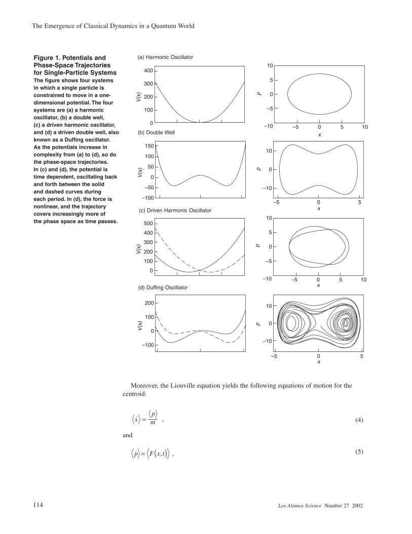
change in time. The resulting curve is called a trajectory in phase space (see Figure 1).The axes of phase space delineate the possible spatial and momentum coordinates thatthe single particle can take. A classical particle’s state is given at any time by a point inphase space, and its motion therefore traces out a curve, or trajectory, in phase space.

By contrast, the state of a quantum particle is not described by a single point in phasespace. Because of the Heisenberg uncertainty principle, the position and momentumcannot simultaneously be known with arbitrary precision, and the state of the systemmust therefore be described by a kind of probability density in phase space. Thispseudoprobability function is called the Wigner function and is denoted by fW(x,p). Asexpected for a true probability density, the integral of the Wigner function over positiongives the probability density for p, and the integral over p gives the probability densityfor x. However, because the Wigner function may be negative in places, we should nottry to interpret it too literally. Be that as it may, when we specify the force on the parti-cle, F(x, t), the evolution of the Wigner function is given by the quantum Liouville equa-tion, which is

(3)

Clearly, in order for a quantum particle to behave as a classical particle, we must beable to assign it a position and momentum, even if only approximately. For example, ifthe Wigner function stays localized in phase space throughout its evolution, then thecentroid of the Wigner function1 could be interpreted at each time as the location of theparticle in phase space.

p = F(x,t) = –∂xV(x,t) , .

The Emergence of Classical Dynamics in a Quantum World

1 The centroid of the Wigner function is the point in phase space consisting of the mean values of x and p, that is (⟨x⟩, ⟨p⟩).

114 Los Alamos Science Number 27 2002

Moreover, the Liouville equation yields the following equations of motion for thecentroid:

(4)

and

(5)

The Emergence of Classical Dynamics in a Quantum World

400

300

200

100

0

200

100

0

–100

10

5

0

–5

10

5

0

–5

150

100

50

0

–50

–100

500

400

300

200

100

0

10

0

–10

10

0

–10

–10 –5

–5

0 5

0 5

10

–10 –5

–5

0 5

0

x

p

V(x

)

p

V(x

)

p

V(x

)

p

V(x

)

x

x

x

5

10

Figure 1. Potentials andPhase-Space Trajectoriesfor Single-Particle SystemsThe figure shows four systemsin which a single particle is constrained to move in a one-dimensional potential. The foursystems are (a) a harmonicoscillator, (b) a double well,(c) a driven harmonic oscillator,and (d) a driven double well, alsoknown as a Duffing oscillator.As the potentials increase incomplexity from (a) to (d), so dothe phase-space trajectories.In (c) and (d), the potential istime dependent, oscillating backand forth between the solid and dashed curves during each period. In (d), the force isnonlinear, and the trajectory covers increasingly more of the phase space as time passes.

(a) Harmonic Oscillator

(b) Double Well

(c) Driven Harmonic Oscillator

(d) Duffing Oscillator

Number 27 2002 Los Alamos Science 115

where m is the mass of the particle. This result, referred to as Ehrenfest’s theorem,2 saysthat the equations of motion for the centroid formally resemble the classical ones butdiffer from classical dynamics in that the force F has been replaced with the averagevalue of F over the Wigner function. Suppose again that the Wigner function is sharplypeaked about ⟨x⟩ and ⟨p⟩. In that case, we can approximate ⟨F(x)⟩ as a Taylor seriesexpansion about ⟨x⟩:

(6)

where σx2 is the variance of x so that σx

2 = ⟨(x – ⟨x⟩)2⟩. If the second and higherterms in the Taylor expansion are negligible, the equations for the centroid become

(7)

and

(8)

And these equations for the centroid are identical to the equation of motion for the classi-cal particle! If we somehow arrange to start the system with a sharply localized Wignerfunction, the motion of the centroid will start out by being classical, and Equation (6) indicates precisely how sharply peaked the Wigner function needs to be.

However, the Wigner function of an unobserved quantum particle rarely remainslocalized even if for some reason it starts off that way. In fact, when an otherwise noninteracting quantum particle is subject to a nonlinear force, that is, a force with anonlinear dependence on x, the evolution usually causes the Wigner function to developa complex structure and spread out over large areas of phase space. In the sequence ofplots in Figure 2(a–d), the Wigner function is shown to spread out in phase space underthe influence of a nonlinear force. Once the Wigner function has spread out in this way,the evolution of the centroid bears no resemblance to a classical trajectory.

So, the key issue in understanding the quantum-to-classical transition is the following: Why should the Wigner function localize and stay localized thereafter? As stated in the introduction, this is an outcome of continuous observation (measurement). We therefore now turn to the theory of continuous measurements.

Continuous Measurement

In simple terms, any process that yields a continuous stream of information may betermed continuous observation. Because in quantum mechanics measurement creates an irreducible disturbance on the observed system and we do not wish to disturb the system unduly, the desired measurement process must yield a limited amount of infor-mation in a finite time. Simple projective measurements, also known as von Neumann

F x F x F xxx( ) = ( ) + ( ) +

σ∂

22

2K,

The Emergence of Classical Dynamics in a Quantum World

2 According to Ehrenfest’s theorem, a quantum-mechanical wave packet obeys the equationof motion of the corresponding classical particle when the position, momentum, and forceacting on the particle are replaced by the expectation values of these quantities.

116 Los Alamos Science Number 27 2002

measurements, introduced in undergraduate quantum mechanics courses, are not ade-quate for describing continuous measurements because they yield complete informationinstantaneously. The proper description of measurements that extract information contin-uously, however, results from a straightforward generalization of von Neumann meas-urements (Davies 1976, Kraus 1983, Carmichael 1993). All we need to do is let thesystem interact weakly with another one, such as a light beam, so that the state of theauxiliary system should gather very little information about the main one over shortperiods and thereby the system of interest should be perturbed only slightly. Only a verysmall part of the information gathered by a projective measurement of the auxiliary sys-tem then pertains to the system of interest, and a continuous limit of this measurementprocess can then be taken. By the mid 1990s, this generalization of the standard meas-urement theory was already being used to describe continuous position measurement bylaser beams. In our analysis, we use the methods developed as part of this effort.

A simple, yet sufficiently realistic, analogy to measuring position by direct observa-tion is measuring the position of a moving mirror by reflecting a laser beam off the mir-ror and continuously monitoring the phase of the reflected light. As the knowledge of thesystem is initially imprecise, there is a random component in the measurement record.Classically, our knowledge of the system state may be refined to an arbitrary accuracyover time, and the random component is thereby reduced. Quantum mechanically,

The Emergence of Classical Dynamics in a Quantum World

20

15

10

5

0

–5

–10

–15–20 –15 –10 –5 0

x5 10 15 20

p

15

10

5

0

–5

–10

–15

–20

–25

15

10

5

0

–5

–10

–15

–20

–25–6 –4 –2 0

x2 4 6 –6 –4 –2 0

x2 4 6

–6 –4 –2 0x

2 4 6

p p

20

15

10

5

0

–5

–10

–15

p

t = 0

t = 0.7

t = 0.5

t = 1.0

Figure 2. Evolution of theWigner Function under aNonlinear ForceThese four snapshots showthe Wigner function at differ-ent times during the simula-tions of the Duffing oscillator.At t = 0, the Wigner function is localized around a singlepoint. As time passes,however, the Wigner functionbecomes increasingly delocalized under the nonlin-ear potential of the Duffingoscillator.

The Emergence of Classical Dynamics in a Quantum World

Number 27 2002 Los Alamos Science 117

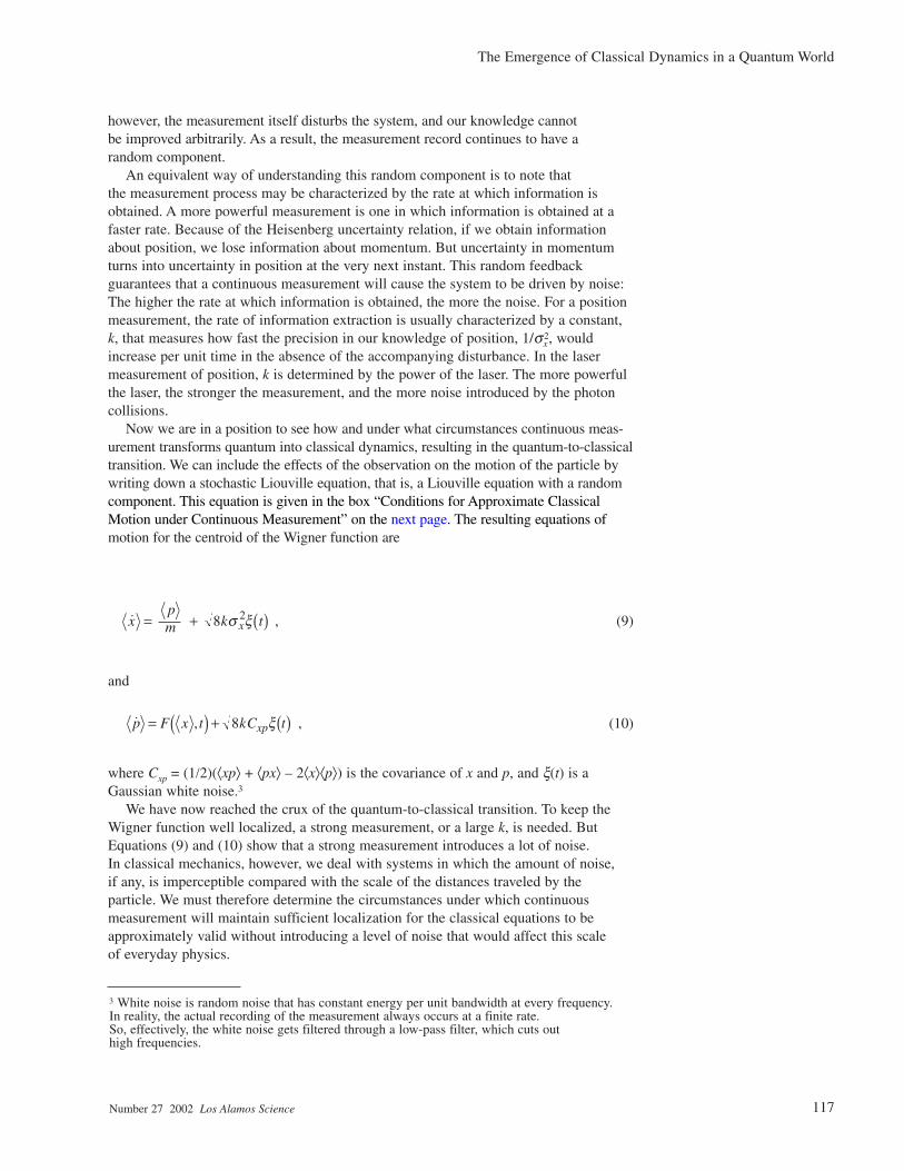
however, the measurement itself disturbs the system, and our knowledge cannot be improved arbitrarily. As a result, the measurement record continues to have a random component.

An equivalent way of understanding this random component is to note that the measurement process may be characterized by the rate at which information isobtained. A more powerful measurement is one in which information is obtained at afaster rate. Because of the Heisenberg uncertainty relation, if we obtain informationabout position, we lose information about momentum. But uncertainty in momentumturns into uncertainty in position at the very next instant. This random feedback guarantees that a continuous measurement will cause the system to be driven by noise:The higher the rate at which information is obtained, the more the noise. For a positionmeasurement, the rate of information extraction is usually characterized by a constant,k, that measures how fast the precision in our knowledge of position, 1/σx

2, wouldincrease per unit time in the absence of the accompanying disturbance. In the lasermeasurement of position, k is determined by the power of the laser. The more powerfulthe laser, the stronger the measurement, and the more noise introduced by the photoncollisions.

Now we are in a position to see how and under what circumstances continuous meas-urement transforms quantum into classical dynamics, resulting in the quantum-to-classicaltransition. We can include the effects of the observation on the motion of the particle bywriting down a stochastic Liouville equation, that is, a Liouville equation with a randomcomponent. This equation is given in the box “Conditions for Approximate ClassicalMotion under Continuous Measurement” on the next page. The resulting equations ofmotion for the centroid of the Wigner function are

(9)

and

(10)

where Cxp = (1/2)(⟨xp⟩ + ⟨px⟩ – 2⟨x⟩⟨p⟩) is the covariance of x and p, and ξ(t) is aGaussian white noise.3

We have now reached the crux of the quantum-to-classical transition. To keep theWigner function well localized, a strong measurement, or a large k, is needed. ButEquations (9) and (10) show that a strong measurement introduces a lot of noise. In classical mechanics, however, we deal with systems in which the amount of noise,if any, is imperceptible compared with the scale of the distances traveled by the particle. We must therefore determine the circumstances under which continuous measurement will maintain sufficient localization for the classical equations to beapproximately valid without introducing a level of noise that would affect this scale of everyday physics.

3 White noise is random noise that has constant energy per unit bandwidth at every frequency.In reality, the actual recording of the measurement always occurs at a finite rate. So, effectively, the white noise gets filtered through a low-pass filter, which cuts out high frequencies.

118 Los Alamos Science Number 27 2002

Conditions for Approximate Classical Motion

The evolution of the Wigner function fW for a single particle subjected to a continuous measurement of position isgiven by the stochastic Liouville equation:

(1)

where F is the force on the particle, ξ is a Gaussian white noise, and k is a constant characterizing the rate of infor-mation extraction. Making a Gaussian approximation for the Wigner function, which according to numerical stud-ies is a good approximation when localization is maintained by the measurement, the equations of motion for thevariances of x and p, σx

2 and σp2, are

(2)

the noise has negligible effect in these equations when the Wigner function stays Gaussian.

First, we solve these equations for the steady state and then impose on this solution the conditions required forclassical dynamics to result. In order for the Wigner function to remain sufficiently localized, the measurement strength k must stop the spread of the wave function at the unstable points, ∂xF > 0:*

(3)

If noise is to bring about only a negligible perturbation to the classical dynamics, it is sufficient that, at a typicalpoint on the trajectory, the measurement satisfy

(4)

where s is the typical value of the system’s action† in units of h. Obviously, as s becomes much larger thanthis relationship is satisfied for an ever-larger range of k. At the spot where this range is

sufficiently large, we obtain the classical limit.

* If the nonlinearity is large on the quantum scale, then 8k needs to be much larger than

irrespective of the sign of ∂xF. This observation does not change the argument in the body of the paper.

† We are assuming that both [mF2/(∂xF)2]|F/p| and E |p/4F| evaluated at a typical point of the trajectory are comparable to the

action of the system, and we define that action to be hs.

82

2k

F

F

F

mx x>> ∂ ∂

.

1

h ∂ ∂x xF F m F2 4( ) ≥ ,

∂x F mF2 2 24( ) h

The Emergence of Classical Dynamics in a Quantum World

The Emergence of Classical Dynamics in a Quantum World

Number 27 2002 Los Alamos Science 119

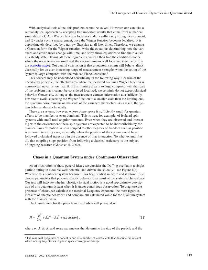
With analytical tools alone, this problem cannot be solved. However, one can take asemianalytical approach by accepting two important results that come from numericalsimulations: (1) Any Wigner function localizes under a sufficiently strong measurement,and (2) under such a measurement, once the Wigner function becomes localized, it isapproximately described by a narrow Gaussian at all later times. Therefore, we assumea Gaussian form for the Wigner function, write the equations determining how the vari-ances and covariances change with time, and solve those equations to find their valuesin a steady state. Having all these ingredients, we can then find the conditions underwhich the noise terms are small and the system remains well localized (see the box onthe opposite page). Our central conclusion is that a quantum system will behave almostclassically for an ever-increasing range of measurement strengths when the action of thesystem is large compared with the reduced Planck constant h.

This concept may be understood heuristically in the following way: Because of theuncertainty principle, the effective area where the localized Gaussian Wigner function isnonzero can never be less than h. If this limiting area is so large compared with the scaleof the problem that it cannot be considered localized, we certainly do not expect classicalbehavior. Conversely, as long as the measurement extracts information at a sufficientlylow rate to avoid squeezing the Wigner function to a smaller scale than the limiting one,the quantum noise remains on the scale of the variances themselves. As a result, the sys-tem behaves almost classically.

There are systems, however, whose phase space is sufficiently small for quantumeffects to be manifest or even dominant. This is true, for example, of isolated spin systems with small total angular momenta. Even when they are observed and interact-ing with the environment, these spin systems are expected to be indescribable by theclassical laws of motion. A spin coupled to other degrees of freedom such as positionis a more interesting case, especially when the position of the system would have followed a classical trajectory in the absence of that interaction. To what extent, if atall, that coupling stops position from following a classical trajectory is the subject of ongoing research (Ghose et al. 2002).

Chaos in a Quantum System under Continuous Observation

As an illustration of these general ideas, we consider the Duffing oscillator, a singleparticle sitting in a double-well potential and driven sinusoidally—see Figure 1(d). We chose this nonlinear system because it has been studied in depth and it allows us tochoose parameters that produce chaotic behavior over most of the system’s phase space.Our test will indicate whether chaotic classical motion is a good approximate descrip-tion of this quantum system when it is under continuous observation. To diagnose thepresence of chaos, we calculate the maximal Lyapunov exponent, the most rigorousmeasure of chaotic behavior,4 and compare our calculated value for the quantum systemwith the classical value.

The Hamiltonian for the particle in the double-well potential is

(11)

where m, A, B, Λ, and ω are parameters that determine the size of the particle and the

4 The maximal Lyapunov exponent is one of a number of coefficients that describe the rates atwhich nearby trajectories in phase space converge or diverge.

The Emergence of Classical Dynamics in a Quantum World

spatial extent of the phase space. The action should be large enough so that the particlecan behave almost classically, yet small enough to illustrate how tiny it needs to bebefore quantum effects on the particle become dominant. Bearing this requirement inmind, we choose a mass m = 1 picogram, a spring constant A = 0.99 piconewton permeter, a nonlinearity A/B = 0.02 square micrometer, a peak driving force ofλ = 0.03 attonewton, and a driving frequency ω = 60 rad per second. Because of theweakness of the nonlinearity, the distance between the two minima of the double well is only about 206 nanometers, and the height of the potential is only 33 nano-electron-volts. The frequency of the driving force is 10 hertz. For these values, a measurementstrength k of 93 per square picometer per second, which corresponds to a laser power ofabout 0.24 microwatt, is adequate to keep the motion classical, or the Wigner functionwell localized.

To study the system numerically, we allow the particle’s Wigner function to evolveaccording to the stochastic Liouville equation for approximately 50 periods of the driving force and then check that it remains well localized in the potential. We find,indeed, that the width of the Wigner function in position (given by the square root of the position variance σx

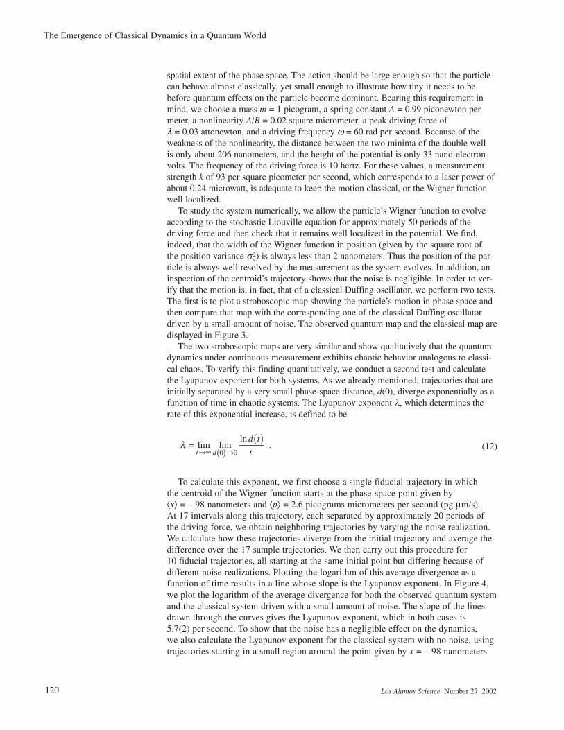
2) is always less than 2 nanometers. Thus the position of the par-ticle is always well resolved by the measurement as the system evolves. In addition, aninspection of the centroid’s trajectory shows that the noise is negligible. In order to ver-ify that the motion is, in fact, that of a classical Duffing oscillator, we perform two tests.The first is to plot a stroboscopic map showing the particle’s motion in phase space andthen compare that map with the corresponding one of the classical Duffing oscillatordriven by a small amount of noise. The observed quantum map and the classical map aredisplayed in Figure 3.

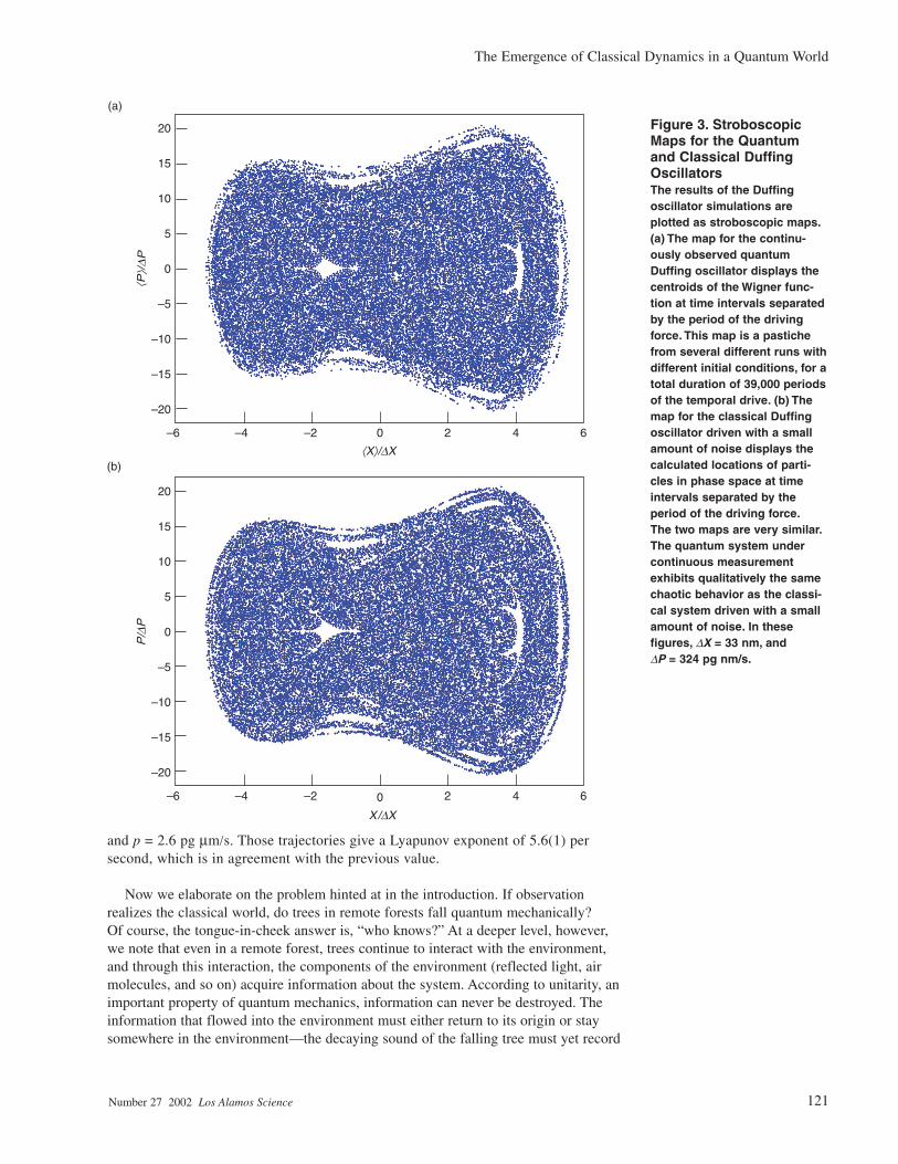
The two stroboscopic maps are very similar and show qualitatively that the quantumdynamics under continuous measurement exhibits chaotic behavior analogous to classi-cal chaos. To verify this finding quantitatively, we conduct a second test and calculatethe Lyapunov exponent for both systems. As we already mentioned, trajectories that areinitially separated by a very small phase-space distance, d(0), diverge exponentially as afunction of time in chaotic systems. The Lyapunov exponent λ, which determines therate of this exponential increase, is defined to be

(12)

To calculate this exponent, we first choose a single fiducial trajectory in which the centroid of the Wigner function starts at the phase-space point given by ⟨x⟩ = – 98 nanometers and ⟨p⟩ = 2.6 picograms micrometers per second (pg µm/s). At 17 intervals along this trajectory, each separated by approximately 20 periods ofthe driving force, we obtain neighboring trajectories by varying the noise realization. We calculate how these trajectories diverge from the initial trajectory and average thedifference over the 17 sample trajectories. We then carry out this procedure for10 fiducial trajectories, all starting at the same initial point but differing because ofdifferent noise realizations. Plotting the logarithm of this average divergence as afunction of time results in a line whose slope is the Lyapunov exponent. In Figure 4,we plot the logarithm of the average divergence for both the observed quantum systemand the classical system driven with a small amount of noise. The slope of the linesdrawn through the curves gives the Lyapunov exponent, which in both cases is5.7(2) per second. To show that the noise has a negligible effect on the dynamics,we also calculate the Lyapunov exponent for the classical system with no noise, usingtrajectories starting in a small region around the point given by x = – 98 nanometers

120 Los Alamos Science Number 27 2002

The Emergence of Classical Dynamics in a Quantum World

Number 27 2002 Los Alamos Science 121

and p = 2.6 pg µm/s. Those trajectories give a Lyapunov exponent of 5.6(1) per second, which is in agreement with the previous value.

Now we elaborate on the problem hinted at in the introduction. If observation realizes the classical world, do trees in remote forests fall quantum mechanically? Of course, the tongue-in-cheek answer is, “who knows?” At a deeper level, however,we note that even in a remote forest, trees continue to interact with the environment,and through this interaction, the components of the environment (reflected light, airmolecules, and so on) acquire information about the system. According to unitarity, animportant property of quantum mechanics, information can never be destroyed. Theinformation that flowed into the environment must either return to its origin or staysomewhere in the environment—the decaying sound of the falling tree must yet record

20

15

10

5

0

–5

–10

–15

–20

–6 –4 –2 2 4 6

20

15

10

5

0

–5

–10

–15

–20

–6 –4 –2 0

0

2 4 6

Figure 3. StroboscopicMaps for the Quantumand Classical DuffingOscillatorsThe results of the Duffing oscillator simulations are plotted as stroboscopic maps.(a) The map for the continu-ously observed quantumDuffing oscillator displays thecentroids of the Wigner func-tion at time intervals separatedby the period of the drivingforce. This map is a pastichefrom several different runs withdifferent initial conditions, for atotal duration of 39,000 periodsof the temporal drive. (b) Themap for the classical Duffingoscillator driven with a smallamount of noise displays thecalculated locations of parti-cles in phase space at timeintervals separated by theperiod of the driving force.The two maps are very similar.The quantum system undercontinuous measurementexhibits qualitatively the samechaotic behavior as the classi-cal system driven with a smallamount of noise. In these figures, ∆X = 33 nm, and∆P = 324 pg nm/s.

(a)

(b)

The Emergence of Classical Dynamics in a Quantum World

its presence faithfully, albeit perhaps only in a shaken leaf. And herein lies the key tounderstanding the unobserved: If a sufficiently motivated observer were to coax theinformation out of the environment, that action would become an act of continuousmeasurement of the current happenings even though actually performed in the future.But since the current state of affairs can’t be influenced by what anyone does in thefuture, the behavior of the system at present cannot contradict anything that such a classical record could possibly postdict.

If the motion is not observed, no one knows which of the possible paths the objecttook, but the rest of the universe does record the path, which could, therefore, be consid-ered as classical as any (Gell-Mann and Hartle 1993). All that happens when there is noobserver is that our knowledge of the motion of the object is the result of averaging over all the possible trajectories. In that case, we are forced to describe the state of thesystem as being given by a probability distribution in phase space since we no longerknow exactly where the system is as it evolves. This observation is, however, just as truefor a (noisy) classical system as it is for a quantum system.

The Connection to the Theory of Decoherence

We can now explain how the analysis presented here relates to a standard approach to the quantum-to-classical transition often referred to as decoherence. The procedureemployed in decoherence theory is to examine the behavior of the quantum system coupled to the environment by averaging over everything that happens to the environ-ment. This procedure is equivalent to averaging over all the possible trajectories that the particle might have taken, as explained above. Thus decoherence gives the evolutionof the probability density of the system when no one knows the actual trajectory. The relevant theoretical tools for understanding this process were first developed andapplied in the 1950s and 1960s (Redfield 1957, Feynman and Vernon 1963), but morerecent work (Hepp 1972, Zurek 1981, 1982, Caldeira and Leggett 1981, 1983a, 1983b,

122 Los Alamos Science Number 27 2002

0

–2

–4

–6

–8

0

–2

–4

–6

–80 2 4

Time (a. u.)6 8

⟨ ln(

∆/∆ 0)

⟩⟨ l

n(∆/

∆ 0) ⟩

Figure 4. LyapunovExponents for theQuantum and ClassicalDuffing OscillatorsIn order to calculate theLyapunov exponents, λ, for (a) a continuously observedquantum Duffing oscillator and (b) a classical Duffingoscillator driven with a smallamount of noise, we plotagainst time the logarithm ofthe average separation of trajectories that begin veryclose together. The parametersdefining the oscillator—thecontinuous-measurementstrength in the quantum system and the noise in the classical system—are detailedon pages 119-–120 of this article. The slope of the linedrawn through the curvesgives the Lyapunov exponent,which in both cases isλ = 0.57(2). Also in both cases,∆0 = 33 nm.

(a)

(b)

The Emergence of Classical Dynamics in a Quantum World

Number 27 2002 Los Alamos Science 123

Joos and Zeh 1985) was targeted at condensed-matter systems and a broader under-standing of quantum measurement and quantum-classical correspondence. It was foundthat averaging over the environment or over the equivalent, unobserved, noisy classicalsystem gives the same evolution (Habib et al. 1998). In this classical counterpart, differ-ent realizations of noise give rise to slightly different trajectories, and in a chaotic sys-tem, these trajectories diverge exponentially fast. As a result, probability distributionsobtained by averaging over the noise tend to spread out very fast, and our knowledge ofthe system state is correspondingly reduced. In other words, discarding the informationthat is contained in the environment or, equivalently, the measurement record, as averag-ing over these data implies, leads to a rapid loss of information about the system. Thisincreasing loss of information, characterized by a quantity called entropy, can then beused to study the phenomenon of chaos with varying degrees of rigor.

Averaging over the environment to produce classical probability distributions was,however, not completely satisfactory. Not only does this averaging procedure not allowus to calculate trajectory-based quantities, but it also restricts our predictions to thosederivable by knowing only the probability densities at various times. But classicalphysics is much more powerful than that—it can predict the outcome of many “if ... then” scenarios. If I randomly throw a ball in some direction, the probability of it landing in any direction around me is the same, but if you see the ball north ofme, you can predict with pretty good certainty that it won’t land south of me. In theclassical world, such correlations are numerous and varied, and the measurementapproach we have taken here completes our understanding of the quantum-to-classicaltransition by treating all correlations on an equal footing. It is easy to see, however,that if the continuous measurement approach has to get all the correlations right, itmust per force get the decoherence of probability densities right!

The realization that continuous measurement was the key to understanding the quantum-to-classical transition has emerged only in the last decade. First introduced in a paper by Spiller and Ralph (1994), this idea was then mentioned again by MartinSchlautmann and Robert Graham (1995). Subsequently, the idea was developed in a col-lection of papers (Schack et al. 1995, Brun et al. 1996, Percival and Strunz 1998, Strunzand Percival 1998). However, the scientific community was slow to pick up on thiswork, possibly because the authors used a stochastic model referred to as quantum statediffusion, which may have obscured somewhat the measurement interpretation. In 2000,we published the results presented in this article, namely, analytic inequalities that deter-mine when classical motion will be achieved for a general single-particle system, andshowed that the correct Lyapunov exponent emerges (Bhattacharya et al. 2000). For thispurpose, we used continuous position measurement, which is ever present in the every-day world and therefore the most natural one to consider. This accumulation of worknow provides strong evidence that continuous observation supplies a natural and satis-factory explanation for the emergence of classical motion, including classical chaos,from quantum mechanics. In addition, such an analysis also makes clear that the specificmeasurement model is not important. Any environmental interaction that provides suffi-cient information about the location of the system in phase space will induce the transi-tion in macroscopic systems. Recently, Andrew Scott and Gerard Milburn (2001) haveanalyzed the case of continuous joint measurement of position and momentum and ofmomentum alone, and they verified that classical dynamics emerges in the same way asdescribed in Bhattacharya et al. (2000). �

124 Los Alamos Science Number 27 2002

Further Reading

Bhattacharya, T., S. Habib, and K. Jacobs. 2000. Continuous Quantum Measurement and the Emergence of Classical Chaos. Phys. Rev. Lett. 85: 4852.

Brun, T. A., I. C. Percival, and R. Schack. 1996. Quantum Chaos in Open Systems: A Quantum State Diffusion Analysis. J. Phys. A 29: 2077.

Caldeira, A. O., and A. J. Leggett. 1981. Influence of Dissipation on Quantum Tunneling in Macroscopic Systems. Phys. Rev. Lett. 46: 211.

———. 1983a. Quantum Tunneling in a Dissipative System. Ann. Phys. (N.Y.) 149: 374.———. 1983b. Path Integral Approach to Quantum Brownian-Motion. Physica A 121: 587.Carmichael, H. J. 1993. An Open Systems Approach to Quantum Optics. Berlin: Springer-Verlag.Davies, E. B. 1976. Quantum Theory of Open Systems. New York: Academic Press.DeWitt, B. S., and N. Graham, Eds. 1973. The Many-Worlds Interpretation of Quantum Mechanics.

Princeton: Princeton University Press.Einstein, A. 1917. On the Quantum Theorem of Sommerfield and Epstein. Verh. Dtsch. Phys. Ges.

19: 434. Feynman, R. P., and F. L. Vernon. 1963. The Theory of a General Quantum System Interacting with

a Linear Dissipative System. Ann. Phys (N. Y.) 24: 118.Gell-Mann, M., and J. B. Hartle. 1993. Classical Equations for Quantum Systems. Phys. Rev. D

47: 3345. Ghose, S., P. M. Alsing, I. H. Deutsch, T. Bhattacharya, S. Habib, and K. Jacobs. 2002. Recovering

Classical Dynamics from Coupled Quantum Systems Through Continuous Measurement. [Online]: http://eprints.lanl.gov (quant-ph/0208064).

Habib, S., K. Shizume, and W. H. Zurek. 1998. Decoherence, Chaos, and the Correspondence Principle. Phys. Rev. Lett. 80: 4361.

Habib, S., K. Jacobs, H. Mabuchi, R. Ryne, K. Shizume, and B. Sundaram. 2002. The Quantum-ClassicalTransition in Nonlinear Dynamical Systems. Phys. Rev. Lett. 88: 040402.

Hepp, K. 1972. Quantum Theory of Measurement and Macroscopic Observables. Helv. Phys. Acta45: 237.

Joos, E., and H. D. Zeh. 1985. The Emergence of Classical Properties through Interaction with the Environment Z. Phys. B 59: 223.

Kraus, K. 1983. States, Effects, and Operations: Fundamental Notions of Quantum Theory. Berlin:Springer-Verlag.

Landau, L. D., and E. M. Lifshitz. 1965. Quantum Mechanics: Non-relativistic Theory. New York:Pergamon Press.

———. 1980. Statistical Physics. New York: Pergamon Press. Omnès, R. 1994. The Interpretation of Quantum Mechanics. Princeton: Princeton University Press.Percival, I. C., and W. T. Strunz. 1998. Classical Dynamics of Quantum Localization. J. Phys. A

31: 1815.Poincaré, H. New Methods of Celestial Mechanics. 1992. Edited by D. L. Goroff. New York: Springer.Redfield, A. G. 1957. Theory of Relaxation Processes in Advances in Magnetic Resonance.

IBM J. Res. Dev. 1: 19.Schack, R., and C. M. Caves. 1999. Classical Model for Bulk-Ensemble NMR Quantum

Computation. Phys. Rev. A 60: 4354. Schack, R., T. A. Brun, and I. C. Percival. 1995. Quantum State Diffusion, Localization and

Computation. J. Phys. A 28: 5401. Schlautmann, M., and R. Graham. 1995. Measurement Trajectories of Chaotic Quantum Systems.

Phys. Rev. E 52: 340. Scott, A. J., and G. J. Milburn. 2001. Quantum Nonlinear Dynamics of Continuously Measured

Systems. Phys. Rev. A 63: 042101. Spiller, T. P., and J. F. Ralph. 1994. The Emergence of Chaos in an Open Quantum System.

Phys.Lett. A 194: 235. Strunz, W. T., and I. C. Percival. 1998. Classical Mechanics from Quantum State

Diffusion—A Phase Space Approach. J. Phys. A 31: 1801. Zurek, W. H. 1981. Pointer Basis of Quantum Apparatus: Into What Mixture Does the Wave

Packet Collapse? Phys. Rev. D 24: 1516. ———. 1982. Environment-Induced Super-selection Rules. Phys. Rev. D 26: 1862. ———. 1991. Decoherence and the Transition to Classical. Phys. Today 44: 36.

The Emergence of Classical Dynamics in a Quantum World

Number 27 2002 Los Alamos Science 125

The Emergence of Classical Dynamics in a Quantum World

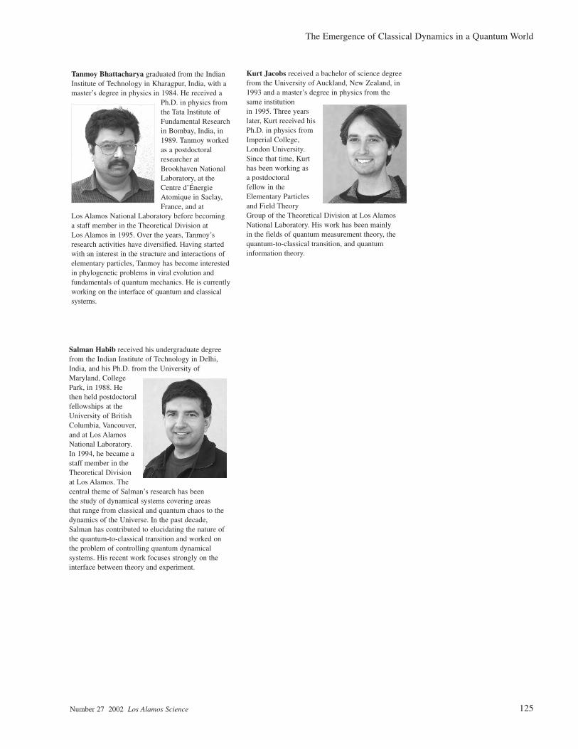
Tanmoy Bhattacharya graduated from the IndianInstitute of Technology in Kharagpur, India, with amaster’s degree in physics in 1984. He received a

Ph.D. in physics fromthe Tata Institute ofFundamental Researchin Bombay, India, in1989. Tanmoy workedas a postdoctoralresearcher atBrookhaven NationalLaboratory, at theCentre d’ÉnergieAtomique in Saclay,France, and at

Los Alamos National Laboratory before becoming a staff member in the Theoretical Division at Los Alamos in 1995. Over the years, Tanmoy’sresearch activities have diversified. Having startedwith an interest in the structure and interactions ofelementary particles, Tanmoy has become interestedin phylogenetic problems in viral evolution and fundamentals of quantum mechanics. He is currentlyworking on the interface of quantum and classicalsystems.

Salman Habib received his undergraduate degreefrom the Indian Institute of Technology in Delhi,India, and his Ph.D. from the University ofMaryland, CollegePark, in 1988. Hethen held postdoctoralfellowships at theUniversity of BritishColumbia, Vancouver,and at Los AlamosNational Laboratory.In 1994, he became astaff member in theTheoretical Divisionat Los Alamos. Thecentral theme of Salman’s research has been the study of dynamical systems covering areas that range from classical and quantum chaos to thedynamics of the Universe. In the past decade,Salman has contributed to elucidating the nature ofthe quantum-to-classical transition and worked onthe problem of controlling quantum dynamical systems. His recent work focuses strongly on theinterface between theory and experiment.

Kurt Jacobs received a bachelor of science degreefrom the University of Auckland, New Zealand, in1993 and a master’s degree in physics from thesame institution in 1995. Three yearslater, Kurt received his Ph.D. in physics fromImperial College,London University.Since that time, Kurthas been working as a postdoctoral fellow in theElementary Particlesand Field TheoryGroup of the Theoretical Division at Los AlamosNational Laboratory. His work has been mainly in the fields of quantum measurement theory, thequantum-to-classical transition, and quantum information theory.