The Emergence of Wage Discrimination in US Manufacturing Joyce Burnette Wabash College Crawfordsville, Indiana 47933 [email protected]October 2009 In spite of the large body of research on labor market discrimination, we are just beginning to map out where and how discrimination operated in the past. One simple answer does not suffice; we must carefully map out what forms discrimination did or did not take for each time and place. In this paper I present evidence on wage discrimination in nineteenth- century US manufacturing, and then examine this evidence as part of a larger picture of the history of discrimination. The results provide further support for Claudia Goldin's claim that wage discrimination emerged around 1900. Economists do not always mean the same thing when they talk about “discrimination.” Fortunately, "discrimination" generally does mean one of a few clearly defined types of discrimination. The two most important models of discrimination are Becker’s wage discrimination model, Bergmann’s occupational crowding model. This paper examines wage discrimination, which occurs if the relative wage paid to females is less than their relative productivity: w f w m < MP f MP m . 1 Even if there is no wage discrimination, other forms of discrimination may exist. Barbara Bergmann’s crowding model provides a model of discrimination that implies no wage discrimination. In the crowding model, women are allowed to enter occupation B, but not occupation A. Women are then “crowded” into occupation B, where the supply of workers is large relative to the demand. Because the marginal product of labor is declining, the large supply 1 Becker defined the market discrimination coefficient as π w π n − π w 0 π n 0 , where π i is the market wage and represents “the equilibrium wage rates without discrimination.” Becker (1971), p. 17. π i 0
Transcript
The Emergence of Wage Discrimination in US Manufacturing
In spite of the large body of research on labor market discrimination, we are just
beginning to map out where and how discrimination operated in the past. One simple answer
does not suffice; we must carefully map out what forms discrimination did or did not take for
each time and place. In this paper I present evidence on wage discrimination in nineteenth-
century US manufacturing, and then examine this evidence as part of a larger picture of the
history of discrimination. The results provide further support for Claudia Goldin's claim that
wage discrimination emerged around 1900.
Economists do not always mean the same thing when they talk about “discrimination.”
Fortunately, "discrimination" generally does mean one of a few clearly defined types of
discrimination. The two most important models of discrimination are Becker’s wage
discrimination model, Bergmann’s occupational crowding model. This paper examines wage
discrimination, which occurs if the relative wage paid to females is less than their relative
productivity:
w f
wm
<MPf
MPm
.1
Even if there is no wage discrimination, other forms of discrimination may exist. Barbara
Bergmann’s crowding model provides a model of discrimination that implies no wage
discrimination. In the crowding model, women are allowed to enter occupation B, but not
occupation A. Women are then “crowded” into occupation B, where the supply of workers is
large relative to the demand. Because the marginal product of labor is declining, the large supply
1 Becker defined the market discrimination coefficient as
πw
π n
−π w
0
π n0
, where π i is the market wage and
represents “the equilibrium wage rates without discrimination.” Becker (1971), p. 17.
π i0
of worker in occupation B leads to a low marginal product of labor and thus a low wage. In
occupation A, where the supply of worker is small relative to the demand, marginal product and
wage are both high. In this model wages are equal to marginal product, so there is no wage
discrimination, but women workers have a low marginal product because they are crowded into
“female” jobs. The method I use will test for wage discrimination, but cannot detect the presence
of occupational crowding. Other studies will be need to test for occupational crowding.2
While the fact that women earned less than men in nineteenth-century US manufacturing
is evident to all, observers have interpreted this fact in very different ways. Some historians
claim that female factory workers were underpaid. Layer (1952, p. 4, 167, 175) claimed that the
labor market for textile workers was not competitive, and that both immigrants and females
earned wages below the competitive level. Gitelman (1967, p. 233) claimed that female cotton
factory workers were paid “a discriminatory wage rate.” Other historians, however, claim that
wages were not discriminatory. In her study of the Amoskeag Co., Hareven (1982, p. 282)
claimed that “Textile work offered significant employment opportunities for women without
wage discrimination.” Paul David (1970, p. 550, 578) suggested that firms did have monopsony
power, but assumed that the female-to-male wage ratio equaled the productivity ratio. Nickless
(1976, p. 107) assumed no monopsony power, and suggested that wages were set at the
competitive level. Some historians suggest that during the late nineteenth century wages were
set at competitive rather than discriminatory levels. Rosenbloom and Sundstrom (2009) suggest
that during the period between the Civil War and World War I labor markets were competitive.
Claudia Goldin (1990, p. 89) concluded that wage discrimination by gender was not important in
nineteenth-century manufacturing, but “emerged sometime between 1890 and 1940 in the white-
collar sector of the economy.”
Most studies that claim to measure wage discrimination do not measure the marginal
product of male and female workers, but use an Oaxaca decomposition to determine whether the
wage gap can be explained by observable characteristics. To calculate the Oaxaca
decomposition, the researcher uses individual-level data on wages to estimate separate wage
equations for men and women. The coefficients from these equations can be used to decompose
2 I have tested for occupational crowding in eighteenth-century English agriculture. I did not find any evidence of crowding there. See Burnette (1996).
the difference in wages into an explained portion and an unexplained portion.3 The explained
portion of the wage gap is the difference in observed characteristics, weighted by the coefficients
of either the male or female wage equation. The remainder of the wage gap is unexplained.
Using this method Goldin (1990, p. 117) found that the unexplained portion of the wage gap rose
from at most 20 percent of the difference in male and female earnings in manufacturing in 1890,
to 55 percent in office work in 1940.”
Unfortunately, the Oaxaca decomposition is a poor measure of wage discrimination. The
unexplained portion of the wage gap is often interpreted as wage discrimination, though, as
Altonji and Blank (1999, p. 3156) note, “This is misleading terminology . . . because if any
important control variables are omitted that are correlated with the included Xs, then the B
coefficients will be affected.” The unexplained portion of the wage gap contains not only wage
discrimination, but also the effects of any omitted variables. If there are any unobserved
variables that affect wages and are correlated with sex, then the unexplained portion of the wage
gap will overestimate wage discrimination. Since the explanatory variables cannot include all
individual characteristics that might be important for productivity, a large portion of the wage
gap may be unexplained simply because we do not have sufficient data to measure productivity,
rather than because of discrimination. Often the unexplained portion of the wage gap is fairly
large, suggesting a wide range of possible levels of wage discrimination, including no wage
discrimination.4
Fortunately, there is a more accurate way to measure wage discrimination. Cross-
sectional firm data can be used to estimate production functions, and to directly estimate the
productivity of female workers relative to male workers. This more accurate measure of
productivity ratio can be compared to the wage ratio to test for wage discrimination. There is
now a small but important body of literature that tests for wage discrimination using productivity
estimates from production functions. Some of these studies are historical, and some use more
recent data.5 Some data sets include information on average male and female wages, and in
3 lnw m − ln w f = (X m − X f )'βm + X f '(βm −β f ) 4 Joyce Jacobsen (1994), p. 317, reports that, in 1990, 71 percent of the gender wage gap was unexplained for whites, and 70 percent for nonwhites. 5 Cox and Nye (1989) examine nineteenth-century France, and McDevitt, Irwin and Inwood (2009) examine Canada in 1870, while Hellerstein and Neumark (1999), Hellerstein, Neumark and Troske (1999) and Haegeland and Klette (1999) examine recent data.
some cases the wage gap must be estimated.6 Some studies conclude that there is wage
discrimination, and some studies conclude that there is no wage discrimination.7 Repeating such
studies for different times and locations will allow us to begin to map historical changes in both
relative female productivity and wage discrimination.
When Claudia Goldin found that wage discrimination increased between the nineteenth
and twentieth centuries, she attributed this change the rise of internal labor markets. She
described the nineteenth century as characterized by spot markets: “Manufacturing jobs and
many others in the nineteenth century were part of what I shall terms the ‘spot market.’ Workers
were generally paid their value to the firm at each instant, or what economists call the value of
labor’s marginal product.”8 This changed in the twentieth century as internal labor markets
replaced spot markets, and women in occupations such as clerical work found their wages
limited by the lack of opportunity for advancement. This hypothesis nicely connects the
emergence of wage discrimination to changes in the economy that seem to have resulted from
the increased importance of firm-specific human capital.
Using a more accurate measure of wage discrimination, this paper confirms Goldin’s
findings that there was little wage discrimination in the nineteenth century. I find no evidence of
wage discrimination between 1833 and 1880. Relative female productivity was increasing in the
textile industry, but wages kept pace with productivity so there is no evidence of wage
discrimination in the antebellum period.
Model
If we assume a Cobb-Douglas production function with homogenous labor, we could
estimate the parameters of the production function by regressing the log of value added on the
logs of the inputs. If labor were homogenous, the production function would be
VA = AK a1 La2 (1a)
or
6 Cox and Nye (1989) use wages reported in the data set, while Hellerstein and Neumark (1999), Hellerstein, Neumark and Troske (1999), Haegeland and Klette (1999), and McDevitt, Irwin and Inwood (2009) must estimate relative wages. 7 Hellerstein, Neumark and Troske (1999) and McDevitt, Irwin, and Inwood (2009) find evidence of wages discrimination, while Cox and Nye (1989) and Hellerstein and Neumark (1999) and Haegeland and Klette (1999) do not. 8 Goldin (1990), p. 114.
(1b) lnVA = ln A + a1 ln K + a2 ln L
where VA is value added (the value of output less the value of raw materials), K is capital, and L
is labor. If labor is not homogenous, however, we need a production function that includes more
than one labor input. One possible way to incorporate different kinds of labor into the
production function is to treat each type of labor as a separate input in the Cobb-Douglas
production function. This was the method used by Cox and Nye (1989) to estimate productivity
in nineteenth-century French manufacturing. They estimated a production function of the form
lnY= ln A + β1 ln M + β2 ln F + β3 ln K
where M is the number of male workers and F is the number of female workers.9 Carden (2004)
used this same model to estimate relative productivity in nineteenth-century US manufacturing.
This production function assumes that the elasticity of substitution between male and female
labor is one. It also assumes that both male and female workers are necessary for production; if
the firm hires zero units of either type of labor, then it cannot produce any output. Because this
second assumption is obviously violated at many firms, I prefer a specification that allows male
and female workers to be perfect substitutes for each other, though not necessarily at a ratio of
one-to-one.
Leonard (1984) included a linear combination of two types of labor as the aggregate labor
input in the Cobb-Douglas production function. He assumed the production function was of the
form
Y = eα1 Kα2 (LA +CLB)α3 (2)
In this production function the two types of labor are perfect substitutes. The parameter C
measures the ratio of the marginal products of the two types of labor, which is a constant and
does not depend on how many workers of each type are employed. While this nested Cobb-
Douglas production function has many advantages, it cannot be estimated by a simple linear
regression.
Various authors have used different techniques to estimate the nested model. Leonard
used a Taylor-series approximation to make the non-linear equation (2) into the linear equation
9 Cox and Nye (1989), p. 907.
lnY =α1 + β1 ln K + β2 ln L + β2(C –1)P (3)
where L is the total number of workers employed, and P is the proportion that are female.
Hellerstein and Neumark (1999) use the same approach to examine relative female productivity
in Israeli manufacturing, and McDevitt, Irwin, and Inwood (2009) use this method to estimate
relative female productivity in Canadian clothing factories. As Leonard notes, this
approximation is closer to the true relationship when P is small and C is close to one. Since
women were a large portion of the workforce in my data set, and I do not expect the productivity
ratio to be close to one, equation (3) is probably not a good approximation of the non-linear
relationship in this case. An alternative is to estimate equation (2) directly using non-linear
regression or maximum likelihood. Other studies have used variants of this approach.
Hellerstein and Neumark (1995) estimate an expanded version of (2) with twelve kinds of labor
categorized by age and occupation. Haegeland and Klette (1999) use maximum likelihood to
estimate the parameters of a nested translog production function.
In this paper I use a nested Cobb-Douglas production function, where the aggregate labor
input is a linear combination of the different types of labor. For the case where there are two
types of labor, M and F, the aggregate labor input is
(4) L* = M + b1F
where L* is the aggregate labor input, M is the number of men, F is the number of women. The
production function is:
VA = CK a1 (M + b1F)a2 (5a)
or lnVA = lnC + a1 lnK + a2 ln(M + b1F ). (5b)
This specification makes it easy to test whether female-male productivity ratio was equal to the
wage ratio. The parameter b1 measures the ratio of the marginal product of a female to the
marginal product of an male:
dVA dFdVA dM
= b1 .
While equation (5) can be used for the 1850 and 1860 censuses, the other data sets
require a specification that allows for three categories of labor. In this case the aggregate labor
input is
(6) L* = M + b1F + b2B
where B is the number of boys for the McLane Report, and the number of children for the 1870
and 1880 censuses. The production function in this case is:
(7a) VA =CK a1 (M + b1F + b2B)a2
or lnVA = lnC + a1 ln K + a2 ln(M + b1F + b2B). (7b)
In this specification the parameter b1 measures the ratio of the marginal product of a female or
adult women to the marginal product of an adult male, and b2 measures the ratio of the marginal
product of a boy, or child, to the marginal product of an adult male.
dVA dFdVA dM
= b1
dVA dBdVA dM
= b2
Both specifications assume that men and women are perfect substitutes, though not necessarily at
a one-for-one ratio. This is reasonable if women and men can be used for the same tasks, but
men produce more output per hour, or can tend a greater number of machines, than women.
The economic history literature has generally favored this specification of the production
function, though usually the parameters b1 and b2 are assumed rather than estimated. Most
studies that have estimated production functions for nineteenth-century manufacturing calculate
an aggregate labor measure by weighting each type of labor by its relative wage, under the
assumption that wages are an accurate measure of productivity. When aggregating the amount
of labor used by manufacturing firms, Sokoloff (1986, p. 702-3) counts an adult woman as the
equivalent of half an adult man because women’s wages were about half of men’s wages.
Females and boys have been treated as equal, in terms of their labor input, to one-half of an adult male employee, with these weights having been drawn from evidence on the relative wages of the groups prevailing near the end of the period.
In a comment on this article, Jeffrey Williamson (1986) questions whether assuming a constant
productivity ratio over time is valid, but does not question the assumption that the wage ratio is
an accurate measure of the productivity ratio. Similarly, Atack, Bateman, and Margo (2003)
assume, based on the wage ratio, that an adult female worker is equal to 60 percent of an adult
male worker in US manufacturing in 1880.10 Ulrich Dorazelski (2004) also constructed a
composite labor measure using the wage ratios to weight female and child labor in his study of
French manufacturing. By estimating the productivity weights, the current paper tests the
assumption that the wage ratio matches to productivity ratio.
Following Aigner, Lovell, and Schmidt (1977), the error term for a production function is
often assumed to have two components, a random error term and an inefficiency term:
yi = f (xi;β) + vi + ui (8)
where vi is a normally distributed error term (such as measurement error) and ui is a nonnegative
error term that indicates if a firm is operating below the production frontier. While (8) can be
estimated by maximum likelihood if an assumption is made about the distribution u, only the
constant term will be biased if the function is estimated by OLS.11 Since I am not concerned
with either the constant term or the efficiency of a particular firm, OLS is sufficient for my
purposes.
1833 McLane Report
The earliest data used in this paper is from a 1833 report to the U.S. House of
Representatives titled Documents relative to the Manufactures in the United States, also known
as the McLane Report because the Secretary of the Treasury Louis McLane collected the returns.
The report was published in 1833, but the data was submitted in the spring of 1832, so the data
set refers to manufacturing in 1831-32. Sokoloff (1986) used data from the McLane Report and
from the 1850 and 1860 censuses to estimate total factor productivity in manufacturing. Goldin
and Sokoloff (1982) the McLane Report and the 1850 census to examine the employment and
wages of female manufacturing workers.
The McLane report includes data on smaller workshop-type establishments, as well as the
more modern factories, though smaller firms are under-represented. Goldin and Sokoloff (1982, 10 See also Atack, Bateman, and Margo, 2005. 11 “if estimation of β alone is desired, all but the coefficient in b corresponding to a column of ones in X is estimated unbiasedly and consistently by least squares.” Aigner, Lovell, and Schmidt, 1977, p. 28.
p. 745) report that the main defect of the data source is that it is not a representative sample of
firms either geographically or in terms of firm size. Neither issue is likely to bias my estimates
of relative female productivity. For the purposes of this paper I have collected two different
samples from this report. The first sample includes all industries, but covers only Massachusetts,
and has 1398 observations. The second sample covers all the states in the McLane report, but
includes only textile firms, and has 427 observations. Each data set includes only firms with
complete information on the output, capital, raw materials, and labor. Massachusetts tended to
give more complete information than other states, leading to an uneven geographical
representation (see Table 1).12 Thus my samples should not be used to draw conclusions about
industry aggregates.
Table 2 provides descriptive statistics for each of these samples. In some cases the
McLane report lists more than one factory together. For example, in Adams, Massachusetts, “2
calico factories” together produced 1.15 million yards of cloth and hired 38 men, 14 boys, and 10
women and girls. In this case the observation includes the aggregate for both firms. The
“singles” samples include only observations that are clearly for one firm only, and the full
sample includes all observations. I test for constant returns to scale before using the full sample.
Output is the dollar value of annual production. Firms reported domestically produced raw
materials separately from imported raw materials, and these are combined into one “Materials”
variable. I will use Value Added, which is equal to Output minus Materials, as my dependent
variable. Capital is the sum of the values of “real estate, buildings, and fixtures”, “tools,
machinery, and apparatus”, and “average stock on hand.”
The McLane Report lists the number of workers employed in three categories; these
categories are: “Average number of males over 16 years old employed”, “Average number of
boys under 16 years of age”, and “Average number of women and girls employed.” This allows
me to estimate the productivity of three separate categories of workers: men, boys, and females.
The “female” category includes both adult women and girls, which may affect the relative
productivity of this group. Female workers in textile factories were relatively young. In the
1830s sixty percent of female workers were under age 20, and 86 percent were under age 25.13
In the full Massachusetts sample 41 percent of the labor force was female. In the textile industry
12 I have also excluded firms which report negative value added or zero capital. 13 Only 14 percent were under age 15, though. Thomas Dublin (1979), p. 31.
about two-thirds of the workers were female. The greater employment of females in textiles is
consistent with other evidence; Thomas Dublin’s study of Hamilton Manufacturing Company in
Lowell found that 85 percent of the workforce was female.14
Wages are reported separately for men, boys, and females, and explicitly state that they
are wages for workers “boarding themselves.” Wages are not reported for every firm in every
category because not every firm hired all three types of labor. The average wage for each type of
labor, then, is based on data collected from less than the full sample of firms. I calculate the
female-to-male wage ratio for each observation that reports both wages. The average of these in
the Massachusetts sample is 0.41, which is the same as wage ratio that Goldin and Sokoloff
report for the McLane Report.15 The wage ratio in the textile industry is slightly higher (0.43).
In the Massachusetts sample boys earned 43 percent as much as men. Unlike females, boys
earned relatively less in the textile industry (0.35).
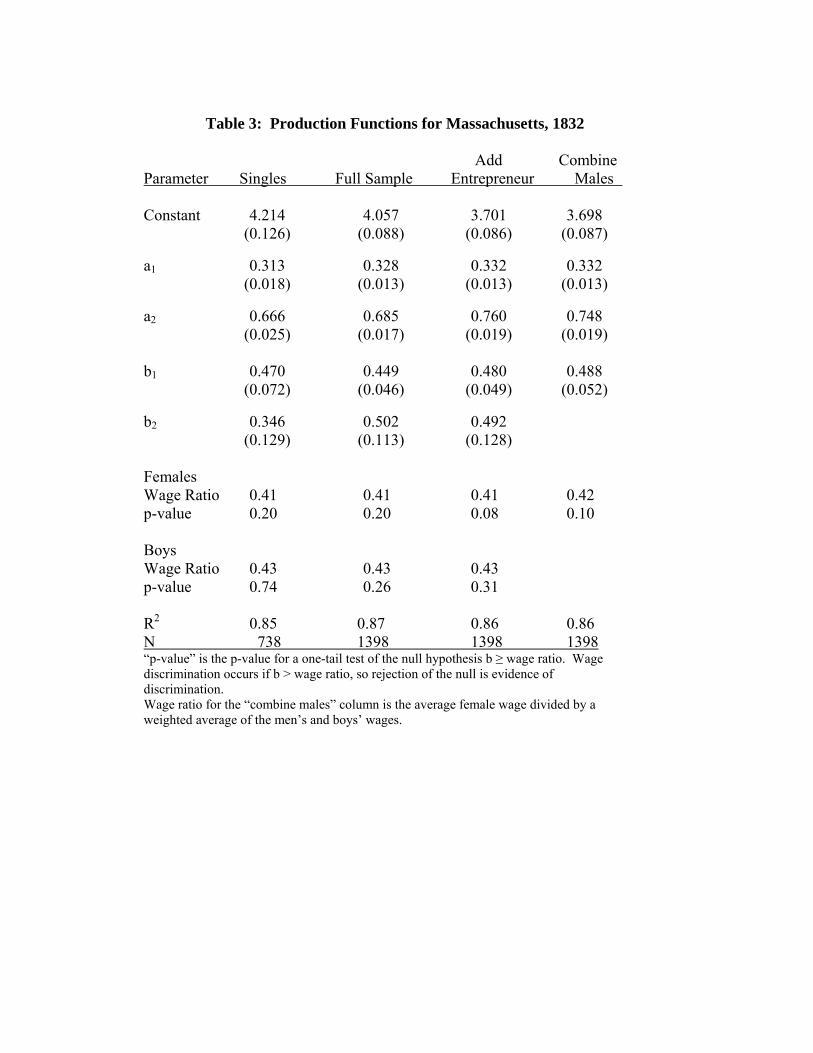
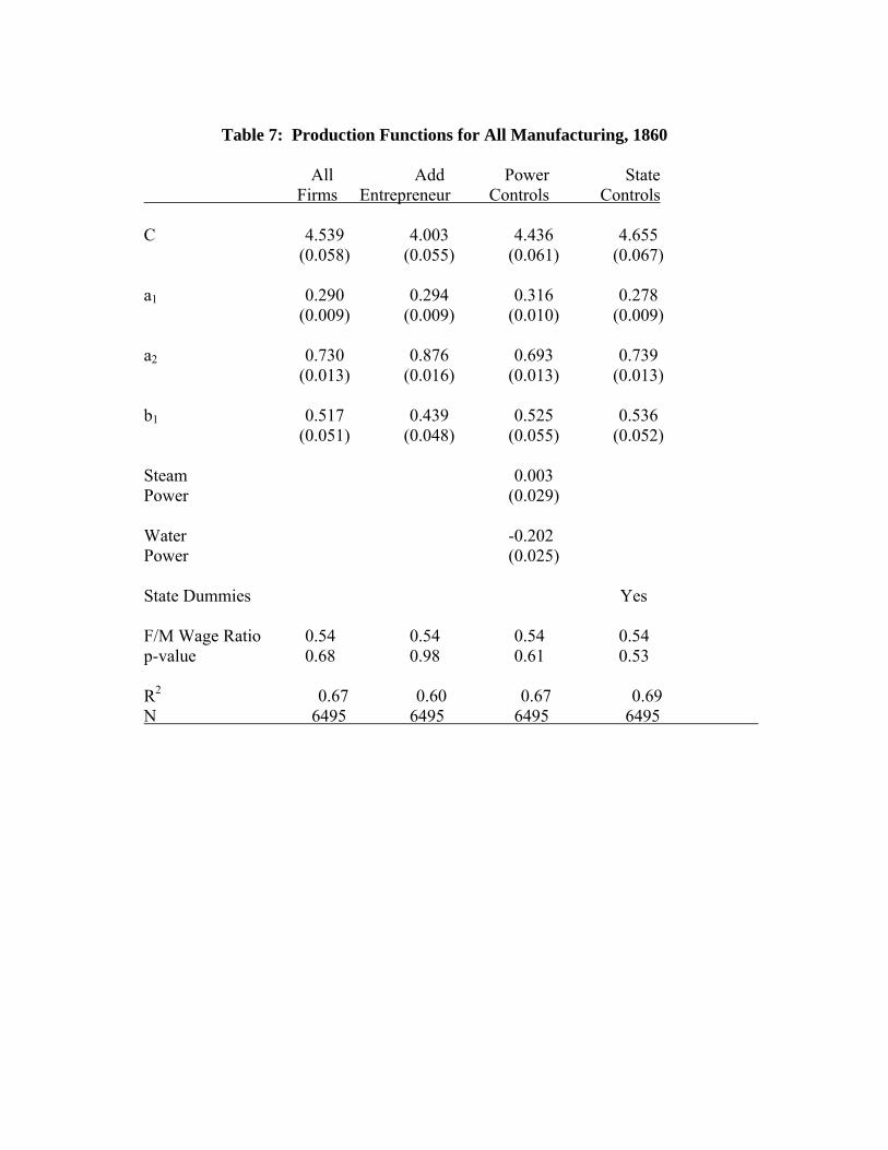
I use this data to estimate the equation lnVAi = lnC + a1 lnKi + a2 ln(Mi + b1Fi + b2Bi) + εi
using non-linear regression. Table 3 presents the results for the Massachusetts sample, including
all industries. The first column presents the results for the singles sample, which includes only
observations known to be for single firms. The results suggest that females were 47 percent as
productive as adult males, and boys were 35 percent as productive. I test for constant returns to
scale by imposing the restriction that a1 + a2 =1, and I cannot reject the null hypothesis that the
restriction is appropriate.16 Since I cannot reject constant returns to scale, I estimate the
production function on the full sample, which also includes observations which aggregate
multiple firms. This estimate suggests that females were 45 percent as productive as men, and
that a boy was half as productive as a man. The estimation in the third column includes an
adjustment for entrepreneurial labor. Sokoloff (1986, p. 686) calculated the aggregate labor
input (total employment) as: TE = M + 0.5 (F+B) + E
14 Thomas Dublin (1979), p. 26. 15 Goldin and Sokoloff (1982), p. 760. Note that the average of the ratios (0.41) is different from the ratio of the average wages (0.38/1.00=0.38) because fewer observations are used for the former. 16 F(1, 733)=1.26.
where M is the number of men, F is the number of females, B is the number of boys, and E is
equal to one. This equation adds one male-equivalent worker for the contribution of the
entrepreneur, who presumably worked at the firm but was not counted as an employee. I used
this variation, with one adjustment: for observations representing multiple firms I added multiple
entrepreneurs. For example, if the observation was listed as “2 calico firms”, then I added two
entrepreneurs. This adjustment does not substantially change the results; in this estimation
females were 48 percent as productive as adults males, while boys were 49 percent as
productive.
All of the coefficients suggest that both females and boys were less productive than adult
males. To test for wage discrimination, we need to compare the estimated productivity ratios to
the observed wage ratios. Table 3 reports p-values for the one-tail test of the hypothesis that the
productivity ratio is less than or equal to the wage ratio. If the productivity ratio is significantly
greater than the wage ratio, then there is wage discrimination. Using a 5% level of significance
we cannot reject the null hypothesis in any case. Using the 10% significance level would lead us
to reject the null for female workers in the third column. I also test the joint hypothesis that b1 =
0.41 and b2=0.43. I estimate a restricted model with aggregate labor equal to
L* = men + entrepreneurs + (0.41*females) + (0.43*boys).
I cannot reject the null hypothesis that the restricted model is a good fit.17 This is essentially a
test of whether the standard method of measuring aggregate labor, which is to use relative wages
to weight the different labor inputs as in equation (8):
M +w f
wm
F +wb
wm
B (8)
is justified. My findings suggest that such a measure of aggregate labor is a good measure of
labor input.
Altonji and Blank (1999, pp. 3197-8) criticize the estimates of Hellerstein, Neumark, and
Troske by noting that firms may choose different gender division of labor as a result of
differences in technology: “the variation across establishments in the makeup of the work force,
particularly in the gender and skill mix, is likely to result mainly from heterogeneity in
production technology.” If being more productive causes firms to hire fewer females, then
females might appear to be less productive than they really are. To check for a relationship
17 F(2, 1393)=1.40.
between productivity and the gender mix of the labor force, I regress the percentage of the firm’s
labor force that is female on residuals from the third regression in Table 3. More productive
firms would have higher-than-expected output, and thus would have positive residuals.
Regression yields the following result:
Percent female = 0.1981 + 0.0005 * Residual R2 = 0.00 (0.0075) (0.0134) The R-squared suggests that there is no relationship between the residuals and the percentage of
the labor force that is female, which suggests that there is no systematic relationship between
firm productivity and the gender mix of the labor force.
Table 4 presents the results from the textile industry. Again, the singles sample includes
only observations that are clearly for a single firm. An F-test cannot reject the hypothesis of
constant returns to scale, so I also use the full sample.18 As above, the third column adds to the
number of men one entrepreneur for each firm in the observation. The estimates suggest that
females were between 40 and 47 percent as productive as adult men, and that boys were between
40 and 44 percent as productive. In no case can we reject the null hypothesis of no wage
discrimination.
The tests above do not provide evidence of wage discrimination, but they also do not tell
us why females were less productivity than adult men. There were many factors contributing to
low female productivity. No doubt the females’ lower average age contributed to the difference,
but differences in skill and strength probably mattered as well. Another characteristic of female
labor affecting their productivity was high turnover. Dublin calculated that 26 percent of
females entered or left employment in a five-week pay period, compared to 21 percent for males.
Because of the high turnover, about one-fifth of the female employees were “spare hands” who
were learning the job. Dublin (1979, pp. 71-2) described the work of the spare hand as basically
a trainee:
the newcomer worked with an experience operative who instructed her in the intricacies of the job. She spelled her partner for shirt stretches of time and occasionally took the place of an absentee. . . After the passage of some weeks or months, when she could handle the normal complement of machinery . . . the sparehand moved into a regular position.
18 F(1, 372)=0.13.
If one-fifth of the female workers were not yet assigned their own machines, this would lead to a
relatively low average output per worker. Differences in the occupations of men and women
also contributed to differences in productivity. Dublin finds that men mainly worked as
overseers, in the repair shop, or tending machines for picking and carding. Men dominated these
positions because of their skills, or, in the case of carding and picking, because they “demanded
considerable strength and endurance and exposed workers to risk of personal injury.”19 Women
tended all the other machines.
Because male workers are divided by age and females are not, the productivity ratios
estimated thus far compare females of all ages to adult males. Boys are clearly less productive
than adult men, and we would expect girls to be less productive than adult women.
Unfortunately, the McLane report does not provide the information necessary to divide females
into two categories. I can, however, combine boys and men into a single category, so that there
are only two kinds of labor, male and female. In the fourth column of Tables 3 and 4 I combine
men and boys into a single category of male workers, and estimate equation (5b) by non-linear
least squares. The female-to-male productivity ratio increases because females are now being
compared to all males, not just adult men. Of course this productivity ratio is influenced by the
fact that the female workers were still relatively young. However, an advantage of the
methodology used here is that I do not have to try to correct for the different characteristics of
the male and female workers. I simply measure the relative productivity of the workers
employed, and check whether the relative productivity of a particular group matched the relative
wage of the same group of workers.
1850 and 1860 Census of Manufacturing
In addition to the McLane Report, I use data from the national samples of the nineteenth-
century censuses of manufacturing compiled by Atack, Bateman and Weiss. Data from the
manufacturing censuses have been used by economic historians to study firm productivity. Craig
and Field-Hendrey (1993) used the 1860 census of to compare productivity in Northern and
Southern manufacturing to productivity in agriculture. Atack, Bateman, and Margo (2003) used
the 1880 census to examine the relationship between output and the length of the working day,
and Atack, Bateman, and Margo (2004) showed that skill intensity (as measured by average
19 Thomas Dublin (1979), p. 65.
wage) decreased with firm size. Because the categories used to report labor change between
1860 and 1870, I will discuss the results from the manufacturing censuses in two parts. This
section will report the results for 1850 and 1860, and the next section will report the results for
1870 and 1880.
The censuses report the value of output, the value of raw materials used, the total capital
invested, and the number of workers. The 1850 and 1860 censuses report the number of workers
in only two categories, men and women. Table 5 shows descriptive statistics for 1850 and 1860,
for all firms, and for textile firms only. Textiles firms were larger than the average
manufacturing firm, and employed a larger portion of women. While the average firm employed
only 9 workers in 1850, the average textile firm employed 41 workers. While the manufacturing
labor force was only 26 percent female, the labor force in textiles was 57 percent female.
The manufacturing censuses do not report a daily or weekly wage, but they do report a
monthly wage bill for male and female workers. I calculate the average monthly wage for each
type of worker by dividing the monthly wage bill by the number of workers at the firm. The
result is noisier than a direct measure of wages, but does give an average wage ratio for the same
firms as are used to estimate productivity. The average ratio of female-to-male wages was 0.49
in 1850 and 0.54 in 1860. Relative female wages were higher in the textile industry, where
females earned 64 percent of the male wage in 1850 and 60 percent in 1860.
To estimate the relative productivity of female workers in 1850 and 1860, I estimate the
Estimating (10) by non-linear least squares gives estimates of b1. Table 13 gives the productivity
ratios estimates from these estimations for all of the data sets used in this paper. The translog
results tell the same story as the Cobb-Douglass results: there is no evidence of wage
discrimination, except for children in 1880.
Trends
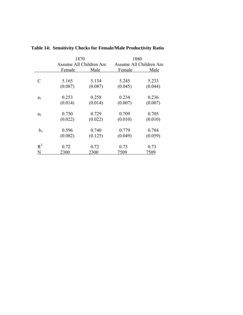
Unfortunately, the differing categories of labor make it difficult to compare productivity
ratios across time. For 1832, 1850, and 1860 the category "female" contained females of all
ages, including girls. Males are separated into men and boys in 1832, but they can easily be re-
combined, producing a female/male productivity ratio comparable to those for 1850 and 1860.
For 1870 and 1880, however, the category “children” contains both boys and girls, so we cannot
re-classify these children. However, we could make different assumptions about the percentage
of children that were female in order to estimate the female-to-male productivity ratio. The two
possible extremes are that all children were boys, and that all children were girls. In Table 14 I
re-estimate the production functions making both of these extreme assumptions. The first and
third columns assume that all children were girls, and add the number of children to the number
of women. The second and fourth columns assume that all children were boys, and adds the
number of children to the number of men. The estimates of relative female productivity under
both of these assumptions should provide bounds for the possible values of the female-to-male
productivity ratio. For 1870, these two assumptions give productivity ratios of 0.60 and 0.74.
For 1880 the two estimates are quite close together, 0.779 and 0.784. These estimates suggest
that relative female productivity in manufacturing increased substantially during the nineteenth
century.
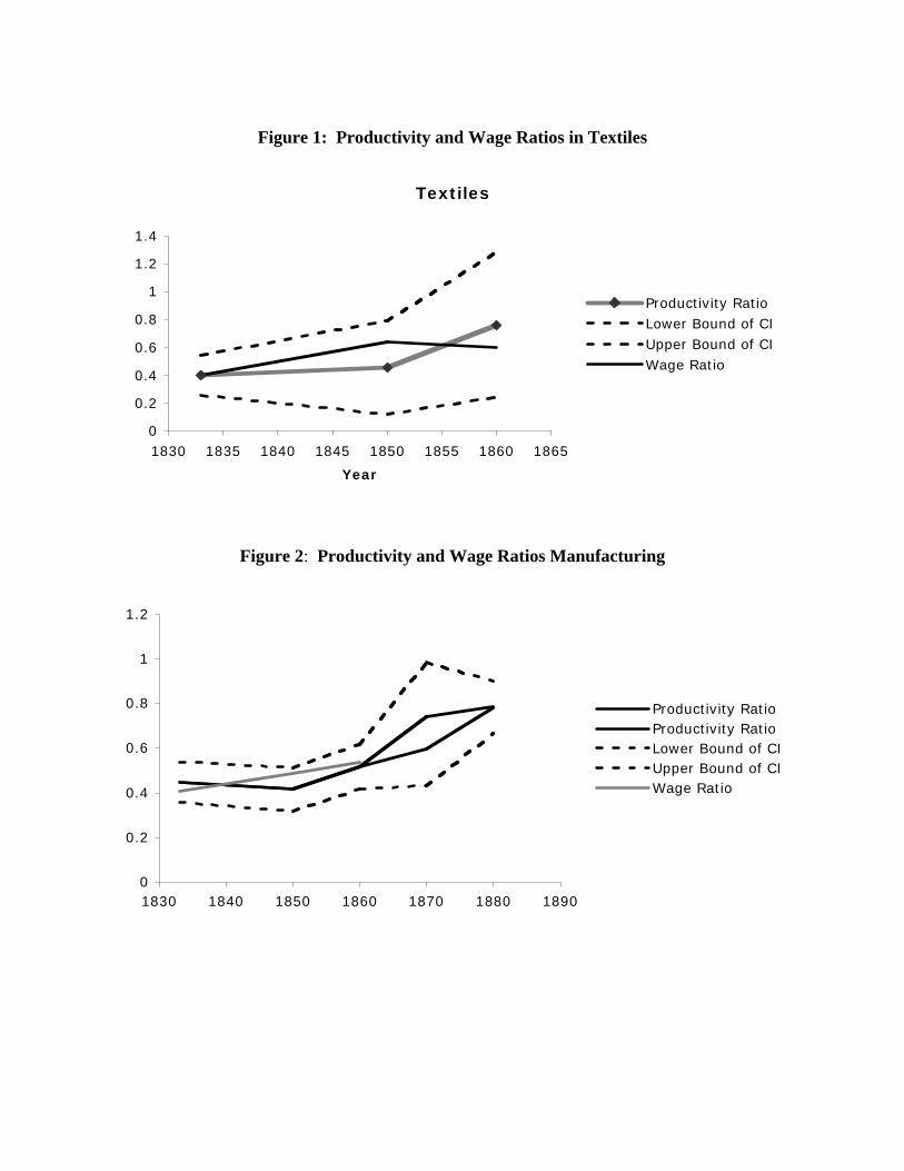
The production functions estimated here reveal interesting differences between textiles
and other industries, and changes over time. In 1850, and particularly in 1860, relative female
productivity was higher in textiles than in manufacturing as a whole, which probably explains
why female employment was so high in textiles. Relative female productivity also increased
over time. Figures 1 and 2 graph the ratios over time. Figure 1 shows wage and productivity
ratios in the textile industry, which are only available until 1860. Figure 2 shows the ratios for
all manufacturing from 1832 to 1880. For 1870 and 1880 I graph the female-male productivity
ratios that result from assuming all children were female, and the ratios that results from
assuming all children were male. Figure 1 shows a pronounced upward trend in relative female
productivity.
The large literature on labor productivity in textiles may provide some clues about why
rising productivity ratio. During the mid-nineteenth century there was an increase in overall
labor productivity in textiles. Lazonick and Brush (1985) attribute this increase to intensification
of work. They note that the native "farmgirls" employed in the 1830s could easily quit in
response to unfavorable working conditions, while the immigrant workers that became more
common in the 1850s did not have the same outside opportunities and were less able to quit.
Reports from female textile workers do suggest that those employed later in the century
seem to have worked harder than those earlier in the century. Harriet Robinson, who wrote a
memoir at the end of the nineteenth century, remembered that when she worked in the mills in
the 1840s the job was not overly taxing:
Though the hours of work were long, they were not over-worked; they were obliged to tend no more looms and frames than they could easily take care of, and they had plenty of time to sit and rest. I have known a girl to sit idle twenty to thirty minutes at a time. They were not driven, and their work-a-day life was made easy.21
However, the factory workers that she interviewed later in the century did not find their job so
easy:
The hours of labor are now less, it is true, but the operatives are obliged to do a far greater amount of work in a given time. They tend so many looms and frames that they have no time to think. They are always on the jump; and so have no opportunity to improve themselves.22
Robinson’s impression is that the work of a female factory hand was greatly intensified.
James Besson, however, does not think the power of the employers changed that much,
and attributed most of the increase productivity between 1835 and 1855 to increases in human
capital. More skilled workers could achieve higher utilization rates, because the could attend to
stops more quickly and effectively. In the 1830s each weaver attended two looms, but over the
course of the century this increased, and by 1902 the average worker attended seven looms.23
Bessen concludes that, while some of this increase was the result of innovations, some of it was
the result of the increased skills of the workers. Because it might take workers up to a year to
21 Robinson (1976), p. 43. 22 Robinson (1976), p. 121-2. 23 Bessen (2008), Figure 2.
reach the highest possible utilization rates for the machines, turnover was an important part of
workers productivity.
Do these theories of labor productivity have any implications for the ratio of female
productivity to male productivity? If the increase in labor productivity occurred among
production workers, then they occurred mainly in the female labor force. In the early period
production workers were almost exclusively female. If productivity increase faster among
female weavers than among male overseers and mechanics, either due to intensification of work
or to human capital acquisition, then we would expect the female/male productivity ratio to rise.
In the middle of the century the gender division of labor changed, as immigrant men were
hired as weavers, a job which had previously been all-female. Gitelman (1967, p. 251) suggests
that this employment pattern, and the lower wage or Irish men, was a result of discrimination.
He claims that Irish males “were more strongly discrimination against within the firm than were
females. Most were consigned to the lowest paying, dirtiest jobs.” While discrimination is one
possible explanation for this pattern, it is also possible that Irish men were hired for the lower-
paying jobs because they had fewer skills than native men. If this were so, then an increase in
the percentage of male workers that were immigrants would reduce average male productivity
and increase the female-male productivity ratio.
Relative female productivity seems to have risen in manufacturing as a whole as well as
in the textile industry. As in the textile industry, both rising female skills and the influx of
unskilled male immigrants may have contributed to this increase.
Conclusion
Since men and women were not equally productive, we can only test for wage
discrimination if we are able to measure the productivity ratio. The estimates of relative
productivity provided in this paper add to a small body of evidence on the male-female
productivity ratio. Table 15 compares the wage and productivity ratios in this paper to results
from various other papers that estimate relative female productivity. The new evidence generally
supports Goldin’s claim that wage discrimination emerged sometime around 1900. I have tested
for wage discrimination and have not found evidence of wage discrimination against women. Of
course, even when there was no wage discrimination, there may have been discrimination in
other forms. Occupational crowding reduces women’s wage without wage discrimination.
By the later twentieth century, though. wage discrimination had come to US
manufacturing. In contrast to Norway and Israel, where there is no evidence of wage
discrimination, US women do seem to have been underpaid in late twentieth-century US
manufacturing. Hellerstein, Neumark, and Troske find evidence of wage discrimination in 1990,
and Leonard finds evidence of wage discrimination in 1966 and 1977.24 Unfortunately, there is
still no evidence for the period between 1860 and 1966, and data limitations make it difficult to
find data for this period. Manuscripts returns of the 1890-1920 censuses of manufacturing do not
survive, and more recent censuses of manufacturing do not report labor by gender. However, it
does appear that wage discrimination appeared in US manufacturing sometime between 1880
and 1966.
Knowing when wage discrimination appeared may help us to understand what caused it.
For most of the nineteenth century, manufacturing employees were paid piece-rate wages and
had short job tenures. These job characteristics led to a spot market, where each worker was
paid his or her current marginal product. As we entered the twentieth century, however, firms
became more anxious to reduce turnover. Owen suggests that technological change, specifically
the automated machinery, increased the importance of firm-specific human capital. More people
were hired into jobs which
required knowledge of particular machines as they were operated in the production process of a given plant; knowledge that constituted firm-specific skills. . . This shift in the skill composition of the work-force toward workers with more firm-specific skills should have led to an increase in the cost of labor turnover to the employer.25
Since turnover was more costly, firms introduced various incentives to discourage workers from
quitting. Firms were successful; quit rates fell from 101 per 100 employees in 1920 to 26 in
1928.26
One of the incentive systems used to reduce turnover was delayed compensation. If
firms paid workers less when first hired, but increased their wages with tenure, workers would
have more incentive to stay with the firm. An increased emphasis on turnover may have led to
statistical discrimination against women, who were expected to have shorter tenures. Firms may
also have decided that men needed greater incentives to stay. Owen finds that male quits were 24 While he does not report the p-value, Leonard does claim that the gender earnings ratio is “significantly less than the productivity ratio.” Leonard (1984), p. 162. 25 Owen (1995), p. 505. 26 Owen (1995), p. 499.
more responsive to market conditions, so firms may have felt more of a need to develop
incentives to keep their male workers. There is some evidence from other the industries that,
when internal labor market policies were in place, women did not have the same opportunities
for advancement as men. Goldin (1990, p. 108) finds that, among American clerical workers
"Each year of total experience augmented male earnings more than female earnings." Men were
assigned to jobs with promotion possibilities and women were not. Similarly, Seltzer and Frank
(2008) find that, among employees of Williams Deacon's Bank in the early twentieth century,
men and women were paid approximately the same salary when first hired, but after about eight
years at the firm a substantial wage gap appeared. Examining Swedish workers in the 1930s,
Svensson (2008) finds that women were assigned to dead-end jobs will little prospect for wage
increases, while men were assigned to jobs with increasing wage profiles.
The change from piece-rate to time-rate payments may have increased wage
discrimination if it was easier to discriminate with time-rate wages. Piece rates were usually the
same for both genders, and any differences would be immediately obvious. However, since male
and female productivity differed, time-rate wages would differ by gender even if there were no
wage discrimination. This would have made wage discrimination less obvious, and perhaps
easier to institute. Evidence on Swedish tobacco workers in 1898 is consistent with the
hypothesis that time-rate wages included more wage discrimination than piece-rate wages.
Stanfors and Karlsson (2008, Table 7) find that, controlling for individual and firm
characteristics, women paid piece-rate wages earned significantly more than women paid time-
rate wages, while for men there was no difference between the two payment types. While more
work remains to be done, it appears that the emergence of wage discrimination was the result of
changes in labor market institutions.
Bibliography Altonji, Joseph, and Blank, Rebecca, 1999, “Race and Gender in the Labor Market,” in Ashenfelter and Card, eds., Handbook of Labor Economics, Elsevier. Atack, Jeremy, Bateman, Fred, and Margo, Robert, 2003, “Productivity in Manufacturing and the Length of the Working Day: Evidence from the 1880 Census of Manufactures,” Explorations in Economic History, 40:170–194. Atack, Jeremy, Bateman, Fred, and Margo, Robert, 2004, “Skill Intensity and Rising Wage Dispersion in Nineteenth-Century American Manufacturing,” Journal of Economic History, 64: 172-192. Atack, Jeremy, Bateman, Fred, and Margo, Robert, 2005, “Capital deepening and the rise of the factory: the American experience during the nineteenth century,” Economic History Review, 68:586-595. Atack, Jeremy, Bateman, Fred and Weiss, Thomas, (2004), National Samples from the Census of Manufacturing, 1850, 1860, and 1870, ICPSR04048, Urbana, IL: University of Illinois, Bloomington, IN: Indiana University, Lawrence, KS: University of Kansas [producers], 2004. Ann Arbor, MI: Inter-University Consortium for Political and Social Research [distributor]. Becker, Gary, 1971, The Economics of Discrimination, 2nd ed., Chicago: University of Chicago Press. Bessen, James, 2003, "Technology and Learning by Factory Workers: The Stretch-Out at Lowell, 1842," Journal of Economics History, 63:33-64. Bessen, James, 2008, "More Machines or Better Machines?" unpublished Burnette, Joyce, 1996, “Testing for Occupational Crowding in Eighteenth-Century British Agriculture,” Explorations in Economic History, 33:319-345. Carden, Art, 2004, “Unequal Pay for Unequal Work in Antebellum America,” mimeo. Cox, Donald and Nye, John Vincent, 1989, “Male-Female Wage Discrimination in Nineteenth-Century France,” Journal of Economic History, 49:903-920. Craig, Lee A. and Elizabeth Field-Hendrey, 1993, “Industrialization and the Earnings Gap: Regional and Sectoral Tests of the Goldin-Sokoloff Hypothesis,” Explorations in Economic History, 30:60-80. David, Paul, 1970, “Learning By Doing and Tariff Protection: A Reconsideration of the Case of the Ante-Bellum United States Cotton Textile Industry,” Journal of Economic History, 30:521-601.
Doraszelski, Ulrich, 2004, “Measuring Returns to Scale in Nineteenth-Century French Industry,” Explorations in Economic History, 41:256-281. Dublin, Thomas, 1979, Women at Work: The Transformation of Work and Community in Lowell, Massachusetts, 1826-1860, New York: Columbia Univ. Press. Gitelman, Howard M, 1967, “The Waltham System and the Coming of the Irish,” Labor History, 8:227-253. Goldin, Claudia, 1990, Understanding the Gender Gap: An Economic History of American Women, Oxford: Oxford Univ. Press. Goldin, Claudia, and Sokoloff, Kenneth, 1982, “Women, Children, and Industrialization in the Early Republic: Evidence from the Manufacturing Censuses,” Journal of Economic History, 42:741–774. Haegeland, Torbjorn, and Klette, Tor Jakob, 1999, “Do Higher Wages Reflect Higher Productivity? Education, Gender and Experience Premiums in a Matched Plant-Worker Data Set” in Haltwanger, Lane, Spletzer, Theeuwes, and Troske, eds., The Creation and Analysis of Employer-Employee Matched Data, Amsterdam: Elsevier, pp. 231–259. Harley, C. Knick, 1992, “International Competitiveness of the Antebellum American Cotton Textile Industry,” Journal of Economic History, 52:559-584. Hareven, Tamara K., 1982, Family Time and Industrial Time: The Relationship Between the Family and Work in a New England Industrial Community, Cambridge Univ. Press. Hellerstein, Judith, and Neumark, David, 1995, “Are Earnings Profiles Steeper Than Productivity Profiles? Evidence from Israeli Firm-Level Data,” Journal of Human Resources, 30:89-112. _____, 1999, “Sex, Wages, and Productivity: An Empirical Analysis of Israeli Firm-Level Data,” International Economic Review, 40:95-123. Hellerstein, Judith, Neumark, David, and Troske, Kenneth, 1999, “Wages, Productivity, and Worker Characteristics: Evidence from Plant-Level Production Functions and Wage Equations,” Journal of Labor Economics, 17:409-446. _____, 2002, “Market Forces and Sex Discrimination,” Journal of Human Resources, 37: 353-380. Jacobsen, Joyce, 1994, The Economics of Gender, Cambridge, MA: Blackwell. Layer, Robert George, 1952, Wages, Earnings, and Output in Four Cotton Textile Companies in New England, 1825-1860, Ph.D diss., Harvard University.
Lazonick, William, and Brush, Thomas, 1985, "The 'Horndal Effect' in Early US Manufacturing," Explorations in Economic History, 22:53-96. Leonard, Jonathan, 1984, “Antidiscrimination or Reverse Discrimination: The Impact of Changing Demographics, Title VII, and Affirmative Action on Productivity,” Journal of Human Resources, 19:145–174. McDevitt, Catherine, Irwin, James, and Inwood, Kris, 2009, "Gender Pay Gap, Productivity Gap and Discrimination in Canadian Clothing Manufacturing in 1870," Eastern Economic Journal, 35:24-36. McLane, Louis, 1969 [1833], Documents Relative to the Manufactures in the United States, New York: Augustus Kelley. Nickless, Pamela, 1976, “Changing Labor Productivity and the Utilization of Native Women Workers in the American Cotton Textile Industry, 1825-1860,” PhD diss., Purdue University. Owen, Laura, 1995, ""Worker Turnover in the 1920s: The Role of Changing Employment Policies," Industrial and Corporate Change, 4:499– Robinson, Harriet, 1976, Loom and Spindle or Life Among the Early Mill Girls, Kailua: Press Pacifica. Rosenbloom, Joshua L., and Sundstrom, William A., 2009, “Labor-Market Regimes in US Economic History,” NBER Working Paper No. 15055 Seltzer, Andrew, and Frank, Jeff, 2008, "Female Salaries and Careers in the British Banking Industry, 1915-41," presented at the Sixth World Congress of Cliometrics, Edinburgh, July 17, 2008. Sokoloff, Kenneth, 1986, “Productivity Growth in Manufacturing during Early Industrialization: Evidence from the American Northeast, 1820-1860,” in Stanley Engerman and Robert Gallman, eds., Long-Term Factors in American Economic Growth, Chicago: University of Chicago Press, pp. 679-729. Stanfors, Maria, and Karlsson, Tobias, 2008, "Gender and the Role of Unions: Earnings Differentials Among Swedish Tobacco Workers in 1898," presented at the Social Science History Association meetings in Miami, Oct. 23, 2008. Svensson, Lars, 2008, "Pay Differentials and Gender Based Promotion Discrimination in a Dual Labour Market: Office Work in Sweden in the mid-1930s," presented at the European Social Science History Conference, Lisbon, March 1, 2008. Williamson, Jeffrey, 1986, “Comment”, in Engerman and Gallman, eds., Long-Term Factors in American Economic Growth, Univ. of Chicago Press, pp. 729–733.
Table 1: Distribution of Textile Firms in the McLane Textile Sample
Percent of Obs. Massachusetts 55.4 New York 19.8 New Hampshire 16.3 Maine 3.7 New Jersey 3.4 Connecticut 0.7 Vermont 0.7
Table 2: Descriptive Statistics, McLane Report
A. Massachusetts Singles Mean Std.Dev. Min Max N Output ($) 23,442 49,560 300 500,000 738 Materials ($) 12,565 26,644 0 367,300 738 Value Added ($) 10,877 22,768 31 251,155 738 Capital ($) 20,240 61,513 120 920,086 738 Men 12.5 20.3 0 200 738 Females 15.6 47.2 0 672 738 Boys 2.9 8.3 0 141 738 Men’s Wage ($) 0.97 0.24 0.33 2.25 716 Female Wage ($) 0.37 0.13 0.02 1.20 369 Boys’ Wage ($) 0.40 0.14 0.11 1.00 260 Wage Ratio F/M 0.41 0.13 0.03 1.15 359 Wage Ratio B/M 0.43 0.15 0.13 1.00 252
B. Massachusetts Full Sample Mean Std.Dev. Min Max N Output ($) 33,939 136,445 180 4,180,000 1398 Materials ($) 17,238 55,204 0 1,190,000 1398 Value Added ($) 16,701 107,631 31 3,863,500 1398 Capital ($) 20,889 57,950 100 920,086 1398 Men 19.2 44.2 0 562 1398 Females 15.9 52.1 0 672 1398 Boys 3.7 12.5 0 200 1398 Men’s Wage ($) 1.00 0.26 0.33 3.5 1346 Female Wage ($) 0.38 0.12 0.02 1.2 553 Boys’ Wage ($) 0.43 0.14 0.11 1.0 467 Wage Ratio F/M 0.41 0.12 0.03 1.2 524 Wage Ratio B/M 0.43 0.14 0.01 1.2 456
C. Textile Singles Mean Std.Dev. Min Max N Output ($) 44,732 86,592 600 800,000 377 Materials ($) 22,566 46,246 60 425,693 377 Value Added ($) 22,166 43,318 297 387,035 377 Capital ($) 71,168 272,332 650 4,200,000 377 Men 17.5 32.2 0 312 377 Females 50.3 114.6 0 1050 377 Boys 8.0 18.0 0 141 377 Men’s Wage ($) 0.96 0.32 0.17 5.00 365 Female Wage ($) 0.39 0.09 0.11 0.83 345 Boys’ Wage ($) 0.33 0.12 0.11 0.87 215 Wage Ratio F/M 0.43 0.15 0.06 1.94 342 Wage Ratio B/M 0.35 0.14 0.13 1.00 212
D. Textile Full Sample
Mean Std.Dev. Min Max N Output ($) 49,003 95,553 240 900,000 427 Materials ($) 26,185 58,384 0 720,530 427 Value Added ($) 22,818 43,103 210 387,035 427 Capital ($) 70,386 257,848 250 4,200,000 427 Men 18.6 34.6 0 312 427 Females 49.6 110.6 0 1050 427 Boys 8.2 18.1 0 141 427 Men’s Wage ($) 0.96 0.31 0.17 5.00 413 Female Wage ($) 0.39 0.08 0.11 0.83 383 Boys’ Wage ($) 0.33 0.12 0.11 0.97 242 Wage Ratio F/M 0.43 0.15 0.06 1.94 379 Wage Ratio B/M 0.35 0.14 0.13 1.01 238
Table 3: Production Functions for Massachusetts, 1832
“p-value” is the p-value for a one-tail test of the null hypothesis b ≥ wage ratio. Wage discrimination occurs if b > wage ratio, so rejection of the null is evidence of discrimination. Wage ratio for the “combine males” column is the average female wage divided by a weighted average of the men’s and boys’ wages.
Table 4: Production Functions for the Textile Industry, 1832
a2 0.798 0.845 0.793 0.816 (0.071) (0.085) (0.074) (0.078) b1 0.763 0.929 0.830 1.032 (0.264) (0.334) (0.295) (0.371) Steam 0.119 Power (0.167) Water -0.063 Power (0.137) State Dummies Yes F/M Wage Ratio 0.60 0.60 0.60 0.60 p-value 0.27 0.16 0.22 0.12
R2 0.83 0.82 0.83 0.83 N 181 181 181 181
Table 10: Descriptive Statistics, Census of Manufactures, 1870 and 1880 Mean Std.Dev. Min Max N 1870 Output ($) 27,405 138,161 45 4,532,422 2484 Materials ($) 15,597 90,712 0 3,050,937 2484 Value Added ($) 11,808 55,780 20 1,481,485 2484 Capital ($) 13,606 85,825 10 3,000,000 2484 Men 9.45 54.76 0 2267 2484 Women 2.56 20.67 0 600 2484 Children 1.58 25.51 0 1200 2484 Wage Bill 5709 29,787 1 936,473 1902 1880 Output ($) 21,434 113,319 100 6,000,000 7512 Materials ($) 14,095 97,208 0 5,600,000 7512 Value Added ($) 7339 26,481 4 1,055,000 7512 Percent of Year 0.85 0.23 0.08 1.00 7512 Adjusted VA 8558 28,717 4 1,055,000 7512 Capital ($) 9111 41,530 10 1,500,000 7512 Men 8.26 29.67 0 1018 7512 Women 2.16 32.87 0 2400 7512 Children 0.54 4.29 0 200 7512 Men, adjusted 8.28 29.79 0 1018 7512 Women, adjusted 2.15 32.98 0 2400 7512 Children, adjusted 0.54 4.30 0 190 7512 Wage Bill 3705 15,152 2 422,530 7246
Adjusted VA is valued added divided by the percent of the year that the factory is in operation. Employment figures are adjusted to a ten-hour day. Adjusted men = men*(hours/10)
Table 11: Estimated Production Functions, 1870 and 1880