The Empirics of Banking Regulation1

Fulbert Tchana Tchana2

Working Paper Number 128

1 I wish to thank Rui Castro, Ren¶e Garcia, Jean Boivin, David Djoumbissie, an anonymous referee, and seminar participants at the Cape Town, Stellenbosch, and Pretoria Universities as well as at the 2008 African Econometric Society conference for valuable comments and suggestions. I also gratefully acknowledge the financial support of the Centre Interuniversitaire de Recherche en Economie Quantitative (CIREQ) and of the URC at the University of Cape Town. 2 School of Economics, University of Cape Town. Email: fulbert.tchanatchana@uct.ac.za

The Empirics of Banking Regulation ∗

Fulbert Tchana Tchana†

School of Economics, University of Cape Town

October 15, 2008

Abstract

This paper empirically assesses whether banking regulation is effective at prevent-ing banking crises. We use a monthly index of banking system fragility, which capturesalmost every source of risk in the banking system, to estimate the effect of regulatorymeasures (entry restriction, reserve requirement, deposit insurance, and capital ade-quacy requirement) on banking stability in the context of a Markov-switching model.Our methodology is less prone to selection and simultaneity bias which are commonin this type of study. We apply this method to the Indonesian banking system, whichhas been subject to several regulatory changes over the last couple of decades, and atthe same time, has experienced a severe systemic crisis. We draw the following findingsfrom this research : (i) entry restriction reduces crisis duration as well as the proba-bility of such an occurrence; (ii) larger reserve requirements reduce crisis duration, butincrease banking instability; (iii) deposit insurance increases banking system stabilityand reduces crisis duration; (vi) capital adequacy requirement improves stability andreduces the expected duration of banking crises. Finally, we find that previous studiespresent a negative simultaneity bias for deposit insurance and a negative selection biasfor capital adequacy requirement.

Keywords: Banking Crises, Banking System Fragility Index, Banking Regulation,Markov Switching Regression.

JEL classification: G21, L16, C25

∗I wish to thank Rui Castro, Rene Garcia, Jean Boivin, David Djoumbissie, an anonymous referee, andseminar participants at the Cape Town, Stellenbosch, and Pretoria Universities as well as at the 2008 AfricanEconometric Society conference for valuable comments and suggestions. I also gratefully acknowledge thefinancial support of the Centre Interuniversitaire de Recherche en Economie Quantitative (CIREQ) and ofthe URC at the University of Cape Town.

†School of Economics, University of Cape Town, Email: fulbert.tchanatchana@uct.ac.za

1

1 Introduction

Banks have always been viewed as fragile institutions that need government help to

evolve in a safe and sound environment. Market failures such as incomplete markets, moral

hazard between banks’ owners and depositors, and negative externalities (like contagion)

have been used to explain this fragility. This has have motivated government regulatory

agencies or central banks to introduce several types of regulatory measures, such as entry

barriers, reserve requirements, and capital adequacy requirements.

Generally, the theoretical effect of any given regulation is mixed. For example, full

deposit insurance helps the banking system to avoid bank panics (see, e.g., Diamond and

Dybvig (1983)). In fact, it provides insurance to depositors that they will in any case obtain

their deposits. However, as all authors acknowledge, it increases the moral hazard issue in

the banking industry. Therefore, the general equilibrium result of deposit insurance is not

as straightforward as one would have thought (see, e.g., Matutes and Vives (1996)).1 For

almost every type of regulation the general equilibrium result is not straightforward on

theoretical grounds (see, e.g., Allen and Gale (2003, 2004), Morrison and White (2005)).

It follows then that the question of the effectiveness of banking regulation is of first-order

empirical importance.

A fair amount of empirical work has already been done on the impact of banking regu-

lation on banking system stability. Barth, Caprio and Levine (2004) assessed the impact of

all available regulatory measures across the world on banking stability. More specifically,

Demirguc-Kunt and Detriagache (2002) focused on the effect of deposit insurance on bank-

ing system stability, while Beck, Demirguc-Kunt and Levine (2006) focused on the impact

of banking concentration. All these studies use discrete regression models such as the logit

model. Although this is an important attempt to empirically test the effect of regulation

on banking system stability, it presents some important limitations: a selection as well as

simultaneity bias and a lack of assessment of the impact of these regulations on banking

crisis duration.

The selection bias comes from the method used to build the banking crisis variable. In

fact, available banking crisis indicators identify a crisis year using a combination of market

events such as closures, mergers, runs on financial institutions, and government emergency

measures. After Von Hagen and Ho (2007), we refer to this approach of dating banking

crisis episodes as the event-based approach.2 This approach identifies crises only when they1Matutes and Vives found that deposit insurance has ambiguous welfare effects in a framework where

the market structure of the banking industry is endogenous.2On this issue of selection bias see von-Hagen and Ho (2007).

2

are severe enough to trigger market events. In contrast, crises successfully contained by

corrective policies are neglected. Hence, empirical work based on the event-based approach

suffers from a selection bias. The simultaneity bias comes from the fact that during periods

of crisis, governments always modify the regulatory framework. Therefore, empirical work

on banking regulation may suffer from simultaneity bias.

The first goal of this paper is to deal with these selection and simultaneity bias problems

by using an alternative estimation method, the Markov-switching regression model (MSM),

to assess the effect of various types of banking regulation on banking system stability.3 The

second goal is to assess the effect of these regulations on crisis duration.

To achieve these goals, we first compute an index of banking system fragility and use

it as the dependent variable to estimate the probability of banking crises. Secondly, we

implement a three-state Markov-switching model, where the three states are: the systemic

crisis state, the tranquil state, and the booming state. We introduce regulatory measures

as explanatory variables of the probability of transition from one state to another to assess

their effect on the occurrence of a systemic banking crisis. We will refer to this method as the

Time-Varying Probability of Transition Markov-Switching Model, hereafter TVPT-MSM.

From the TVPT-MSM, we derive the marginal effect of each regulatory measure on the

probability of being in the systemic banking crisis state. Thirdly, we use this specification

to assess the effect of regulatory measures on banking crisis duration. Fourthly, we carry

out a sensitivity analysis: we first use an alternative index to see if the results are robust;

we also use a Monte Carlo procedure to check the sensitivity of the results to having less

than two states and to having state-dependent standard deviations. Finally, we assess the

importance of selection and simultaneity bias resolved by the TVPT-MSM.

We applied our methodology to an emerging market economy, Indonesia, which has

suffered from banking crises during the period 1980-2003, and where there have been some

dynamics on the regulatory measures during the same period. We focus our analysis on

four major regulatory measures: (i) entry restriction; the removal of entry restriction is

assumed by many authors such as Allen and Herring (2001) to have contributed to the

reappearance of the systemic banking crisis; (ii) deposit insurance, which is supposed to

reduce instability by providing liquidity, therefore reducing the possibility of bank runs.

However, it has been found by many authors to increase the moral hazard problem in the

banking industry; (iii) reserve requirements, which most economists viewed as a tax on the

banking system that can lead to greater instability in the banking system; and (iv) the3In fact, as pointed out by Diebold, Lee and Weinbach (1994), the Markov-switching model is useful

because of its ability to capture occasional but recurrent regime shifts in a simple dynamic econometricmodel.

3

capital adequacy requirement, which is promoted by the Basel Accords and is supposed to

be effective in reducing the probability of a banking crisis.

We find that reducing entry restriction increases the duration of a crisis and the proba-

bility of being in the banking crisis state. The reserve requirement reduces crisis duration

but seems to increase banking fragility. Deposit insurance increases the stability of the In-

donesian banking system and reduces the duration of banking crises. The capital adequacy

requirement improves stability and reduces the expected duration of banking crises. This

later result is obtained when we control for the level of entry barrier.

Finally, we find that previous studies present a negative simultaneity bias for deposit

insurance due to the fact that this policy was adopted and implemented in 1998 during a

crisis period; and a negative selection bias for capital adequacy requirement.

Our paper builds on the previous literature of banking crisis indices and the Markov-

switching regression. The paper most closely related to ours is by Ho (2004), who also

applied the MSM to the research on banking crises. It uses a basic two-state Markov-

switching model to detect episodes of banking crises. However, his paper does not apply

the MSM framework to study the effect of banking regulations on the banking system

stability, which is the main feature we are interested in. The papers by Hawkins and Klau

(2000), Kibritcioglu (2002), and Von-Hagen and Ho (2007) are related in that they build

banking system fragility indices, and use them to identify episodes of a banking crisis.4 The

objective of this method is to construct an index that can reflect the vulnerability or the

fragility of the banking system (i.e., periods in which the index exceeds a given threshold

are defined as banking crisis episodes).

The remainder of this paper is organized as follows. Section 2 presents the TVPT-MSM

and its estimation strategy. Section 3 analyzes the Indonesian banking system. Section 4

empirically assesses the effect of banking regulations on the occurrence and the duration of

banking crises. Section 5 carries out a sensitivity analysis. Section 6 assesses the selection

and simultaneity bias. We conclude in section 7.

2 The Model, Estimation Strategy and Data

To estimate a Markov-switching model we need an indicator that we will use to assess

the state of the banking activity. Therefore, in this section, we first present an index of

banking system fragility, before presenting the TVPT-MSM.4These authors follow the approach taken by Eichengreen, Rose and Wyplosz (1994, 1995, and 1996) for

the foreign currency market and currency crises.

4

2.1 The Banking System Fragility Index

The idea behind the banking system fragility index (hereafter BSFI), introduced by

Kibritcioglu (2003), is that all banks are potentially exposed to three major types of eco-

nomic and financial risk: (i) liquidity risk (i.e., bank runs), (ii) credit risk (i.e., rising of

non-performing loans), and (iii) exchange-rate risk (i.e., bank’s increasing unhedged foreign

currency liabilities).5 The BSFI uses the bank deposit growth as a proxy for liquidity risk,

the bank credit to the domestic private sector growth as a proxy for credit risk, and the

bank foreign liabilities growth as a proxy for exchange-rate risk. Formally, the BSFI is

computed as follows:

BSFIt =NDEPt + NCPSt + NFLt

3with (1)

NDEPt =DEPt − µdep

σdepwhile DEP t=

LDEP t−LDEP t−12

LDEP t−12, (2)

NCPSt =CPSt − µcps

σcpswhile CPSt=

LCPSt−LCPSt−12

LCPSt−12, and (3)

NFLt =FLt − µfl

σflwhile FLt=

LFLt−LFLt−12

LFLt−12. (4)

where µ(.) and σ(.) stand for the arithmetic average and for the standard deviation of these

three variables, respectively. LCPSt denotes the banking system’s total real claims on the

private sector; LFLt denotes the bank’s total real foreign liabilities; and LDEPt denotes

the total deposits of banks. One should notice that nominal series are deflated by using the

corresponding domestic consumer price index.

2.2 The Markov-Switching Model

In this subsection we present and provide the estimation method of our econometric

model.

2.2.1 The Model Setup

We adapt the Garcia and Perron (1996) MSM to assess the state of the banking activity.

To ease the presentation, we present only the model with three states (which happen to be

more appropriate for our data), although we have studied the other specifications. These

three states are : (i) the systemic crisis state with a mean µ1 and variance σ21, (ii) the

tranquil state with a mean µ2 and variance σ22, and (iii) the booming state with a mean

5Demirguc-Kunt, Detragiache and Gupta (2006) have found in a panel of countries, which have sufferedfrom systemic banking crises during the last two decades, that in crises years, one observes an importantdecrease in the growth rate of banks’ deposits and of credit to the private sector.

5

µ3 and a variance σ23.

6 Let y be a banking system fragility index (as provided in the above

subsection). We assume that the index’s dynamics are only determined by its mean and its

variance. We set up the model as follows:

yt = µst + est (5)

where est ∼ iid N(0, σ2st

),

µst = µ1s1t + µ2s2t + µ3s3t,

σ2st

= σ21s1t + σ2

2s2t + σ23s3t,

and sjt = 1, if st = j, and sjt = 0, otherwise, for j = 1, 2, 3. The stochastic process on st can

be summarized by the transition matrix pij,t = Pr[st = j|st−1 = i, Zt], with∑3

j=1 pij,t = 1.

Zt is the vector of N exogenous variables which can affect the transition probability of the

banking crisis. It is a vector of real numbers. The (3X3) transition matrix Pt at time t is

given by

Pt =

p11,t p21,t p31,t

p12,t p22,t p32,t

p13,t p23,t p33,t

. (6)

We assess the effect of regulations on banking crises by assuming that the transition

probability from one state to another is affected by regulatory measures taken by the gov-

ernment such as the entry barrier, the reserve requirement, the deposit insurance, and the

capital adequacy requirement.7 Formally, we assume that for i = 1, 2, 3 and all t,

pij,t =exp(λij,0 +

∑Nk=1 λij,kZkt)

1 + exp(λi1,0 +∑N

k=1 λi1,kZkt) + exp(λi2,0 +∑N

k=1 λi2,kZkt)(7)

for j = 1, 2; while,

pi3,t =1

1 + exp(λi1,0 +∑N

k=1 λi1,kZkt) + exp(λi2,0 +∑N

k=1 λi2,kZkt)(8)

Note that the model specification with constant probability of transition is a special

case of the above model where Zt is the null matrix.

This model is well suited to account for selection bias since it uses a measure of banking

system activity more robust to prompt and corrective action, and also because the Markov-

switching model is an endogenous regime switching model that, according to Maddala6Hawkins and Klau (2000), and Kibritcioglu (2003) argue that banking crises are generally preceded by a

period of high increases of credit to the private sector and/or high increases of deposits and/or high increasesof foreign liabilities. Some studies even labelled the booming state as the pre-crisis state.

7See Filardo (1994) for a deeper assessment of a Markov-switching model with time varying probabilityof transition.

6

(1986), is a good framework for a self-selection model. The TV PT −MSM is also suitable

to account for simultaneity bias since the states of nature and the effect of regulation on

the occurrence of these states are jointly estimated. In other words, the TV PT −MSM is

a type of a simultaneous equations model.

2.2.2 The Estimation Method for the TVPT-MSM

We jointly estimate the parameters in equation (5) and the transition probability pa-

rameters in equation (7) by maximum likelihood.8 For this purpose, we first derive the

likelihood of the model. The conditional joint-density distribution, f , summarizes the in-

formation in the data and explixitly links the transition probabilities to the estimation

method.

If the sequence of states {st} from 0 to T were known, it would be possible to write the

joint conditional log likelihood function of the sequence {yt} as

ln [f(yT , ..., y0|sT , ..., s0, ZT , ..., Z0)] = −T

2ln 2π −

T∑

t=2

{ln(σst) +

{yt − µst}2

2σ2st

}. (9)

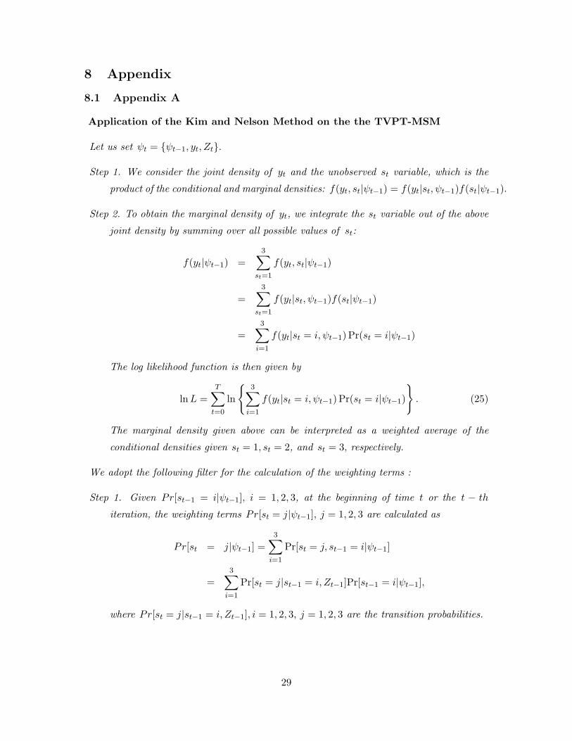
Since st is not observed, but only yt from time 0 to T , we adapt the two-step method of

Kim and Nelson (1999) to determine the log likelihood function. (See details in appendix

A).

2.3 Estimating the Marginal Effect of Regulation on Banking Stability

When the regulatory measures are included in the probability of transition, the result

obtained from the standard Markov-switching estimation is the estimated value of the pa-

rameters defining the transition probabilities. Since many parameters are involved in the

computation of these probabilities of transition, the direct estimates of these parameters

do not tell us the full story about the effect of each regulatory measure on the transition

probability. More importantly, it does not provide an assessment of each regulatory vari-

able on the probability of the banking system being in a given state. In other words, to

obtain the effect of a regulatory measure (zl) on the banking stability one should compute

the marginal effect of each regulation on the probability of the banking system being in

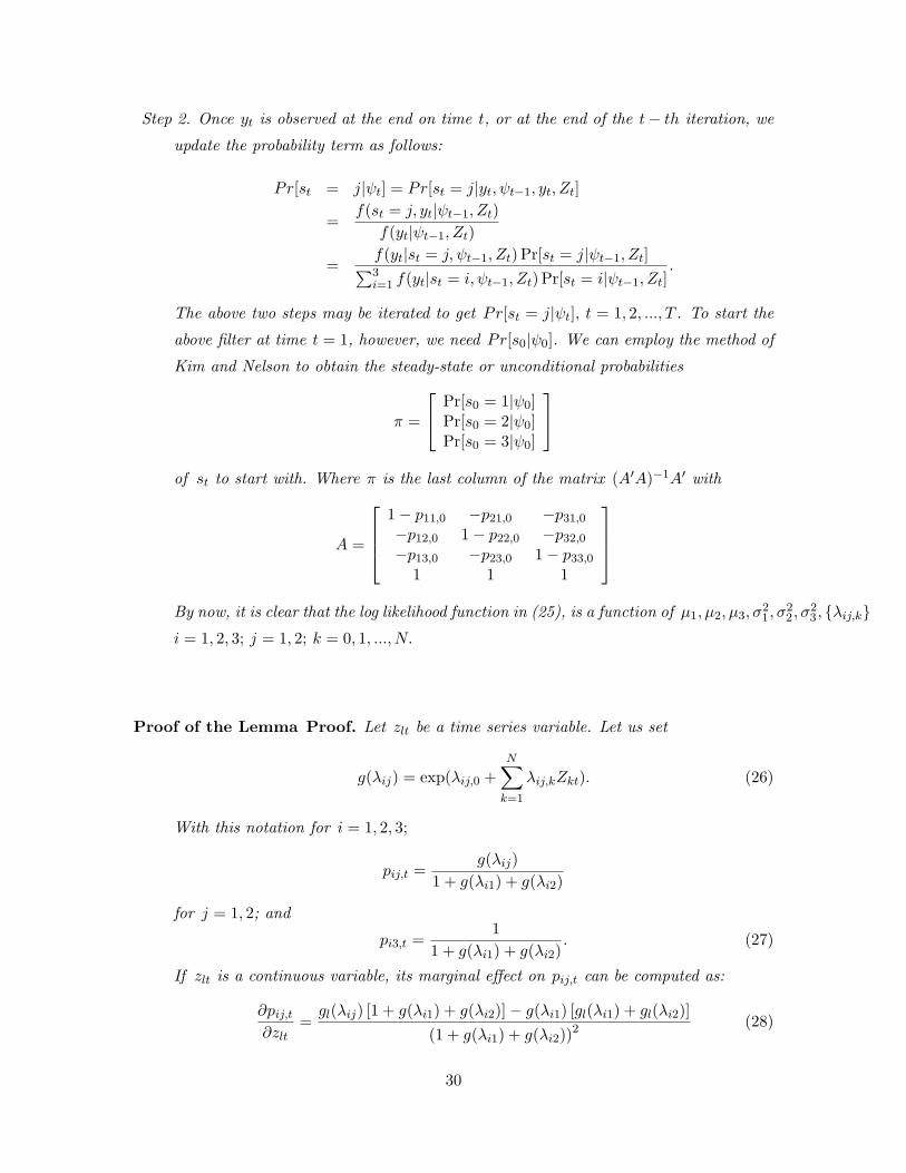
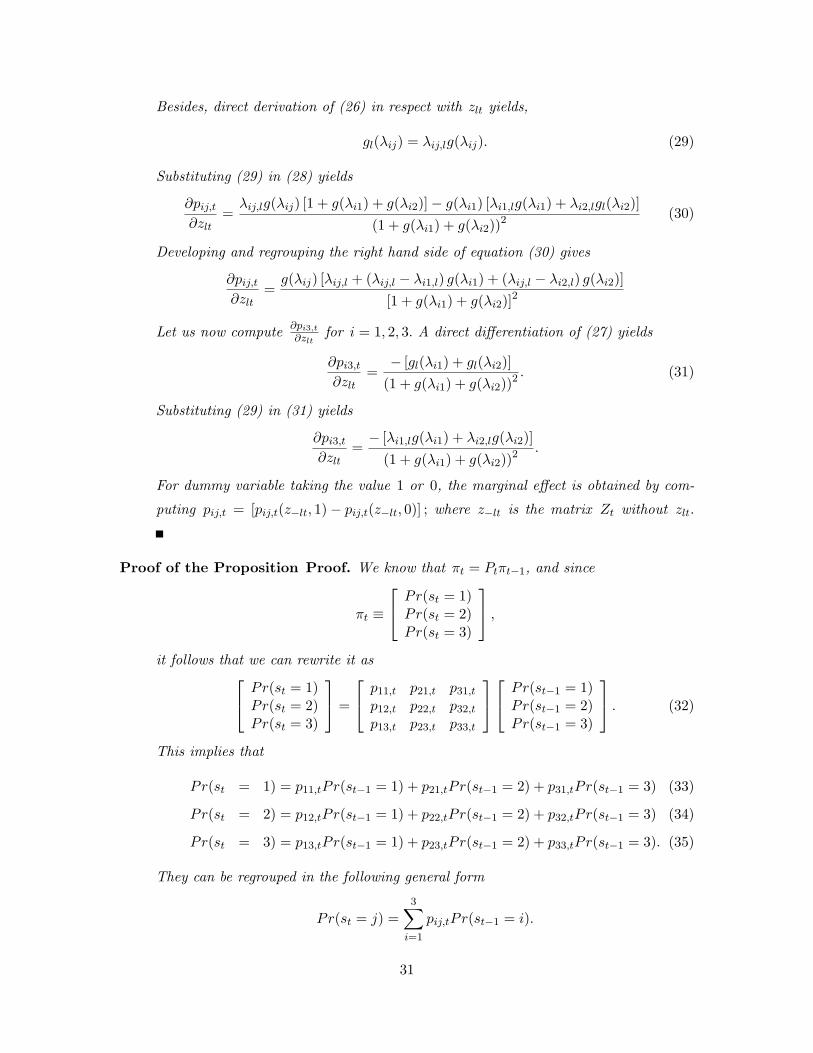
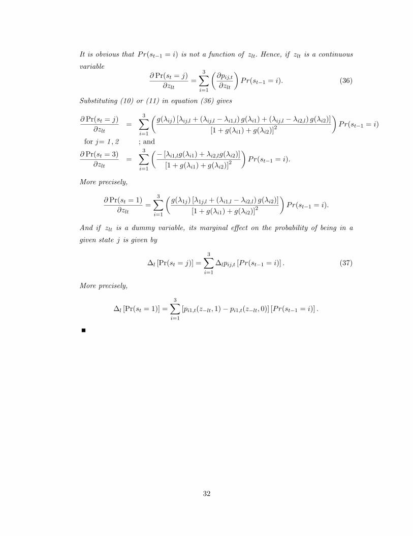
the systemic crisis state. We derive the result in the proposition below, but first present a

lemma that will help in the derivation.8In the MSM literature there are some other estimation techniques for the TVPT-MSM. For example

Diebold, Lee, and Weibach (1994) proposed the EM algorithm to estimate a related model and Filardo andGordon (1993) used a Gibbs Sampler to estimate the same type of model.

7

Lemma Let zlt be a time series variable, if zlt is a continuous variable, the marginal effect

of zlt on pij,t for i = 1, 2, 3 is given by:

∂pij,t

∂zlt=

g(λij) [λij,l + (λij,l − λi1,l) g(λi1) + (λij,l − λi2,l) g(λi2)][1 + g(λi1) + g(λi2)]

2 , (10)

for j = 1, 2; and;∂pi3,t

∂zlt=

− [λi1,lg(λi1) + λi2,lg(λi2)][1 + g(λi1) + g(λi2)]

2 , (11)

with g(λij) = exp(λij,0 +N∑

k=1

λij,kzkt).

Let zlt be a dummy variable, the marginal effect of zlt on pij,t is given by

∆pij,t = [pij,t(z−lt, 1)− pij,t(z−lt, 0)] ; (12)

where z−lt is the matrix Zt without zlt.

Proof. These results are straightforward from a partial differentiation of (7) and (8).

See details in appendix A.

Proposition The marginal effect of any exogenous continuous time series variable

zlt on the probability of the banking system to be in state st = 1 is given by:

∂ Pr(st = 1)∂zlt

=3∑

i=1

g(λij) [λi1,l + (λi1,l − λi2,l) g(λi2)] Pr(st−1 = i)[1 + g(λi1) + g(λi2)]

2 . (13)

The marginal effect of any exogenous dummy variable zlt on the probability of

the banking system to be in state st = 1 is given by:

∆l [Pr(st = 1)] =3∑

i=1

[pi1,t(z−lt, 1)− pi1,t(z−lt, 0)] [Pr(st−1 = i)] . (14)

Proof. The idea of this proof is to compute the unconditional probability of

state st = 1, and then derive it with respect to zlt . Details are available in

appendix A.

We know that a given continuous variable zk has a positive effect on the banking system

stabilization if it has a positive effect on Pr(st = 1). i.e., at any time t, ∂Pr(st=1)∂zkt

≥ 0. Using

the above proposition, this is achieved when for all i

λi1,k ≥ 0, and λi1,k ≥ λi2,k. (15)

8

In other words, the regulatory measure (zk) increases the probability of the banking system

to get into a systemic banking crisis when (15) is met. Conversely, if for all i

λi1,k ≤ 0, and λi1,k ≤ λi2,k (16)

the regulatory measure (zk) reduces the probability of the banking system to suffer a sys-

temic banking crisis.

The other combinations of parameters are difficult to handle analytically, but fortunately

with the above proposition we can compute the marginal effect of each explanatory variable

at its mean. To do this we follow the literature of the discrete variable model, which

computes the marginal effect at the mean of the explanatory variable.We then use the delta

method to compute the standard error of this marginal effect.

2.4 Effect of Regulation on Banking Crisis Duration

A heuristic idea of the effect of a regulatory measure (zk) on the crisis duration is given

by the sign of ∂p11,t

∂zkt. From the above lemma ∂p11,t

∂zkt≥ 0 if

λ11,k ≤ 0, and λ11,k ≤ λ12,k. (17)

It follows that the regulatory measure zk reduces the probability of remaining in state 1, (

i.e., remaining in the banking crisis state) if condition (17) is met. This can be viewed as a

positive effect on the banking crisis duration.

However, to properly assess the expected duration of a given state j, at each time t, we

keep in mind that the adoption of any type of regulation is assumed to be exogenous and

that its adoption is not predictable. We will then consider that the expected duration at

a given point in time is based on the transition probability observed at that time. More

precisely, the expected duration of a given state j, at time t, conditional on the inferred

state (crisis state, tranquil state or booming state, respectively) is given by:

Et(Dj) =∞∑

d=1

dPr(Dj = d|yt−1, Zt) (18)

=∞∑

d=1

d

[Pr(St+d 6= j|St+d−1 = j, Zt)

d−1∏

i=1

Pr(St+i = j|St+i−1 = j, Zt)

]

=∞∑

d=1

d

[(1− Pr(St+d = j|St+d−1 = j, Zt))

d−1∏

i=1

Pr(St+i = j|St+i−1 = j, Zt)

].(19)

Since for all i

Pr(St+i = j|St+i−1 = j, Zt) = Pr(St = j|St−1 = j, Zt), (20)

9

the expected duration is similar to the case of absence of constant probability of transition.

In fact, substituting (20) in (19) yields

Et(Dj) =1

1− Pr(St = j|St−1 = j, Zt). (21)

2.5 Data Sources

We use the International Financial Statistics (IFS) database of the International Monetary

Fund (IMF). More precisely, LCPS is taken from IFS’s line 22D, LFL is taken from line

26C, LDEP is considered as the sum of lines 24 and 25 in the IFS. We deflated nominal

series by using the corresponding domestic consumer price index (CPI) taken from IFS

line 64. The dummy variable for explicit deposit insurance is taken from Demirguc-Kunt,

Kane and Laeven (2006). The reserve requirement is taken from Van’t Dack (1999), and

Barth, Caprio and Levine (2004). The capital adequacy requirement is taken from the

Indonesian Bank Act 2003. The entry restriction variable is constructed based on Abdullah

and Santoso (2001) and Batunanggar (2002).

3 The Background of the Indonesian Banking System

We now apply our estimation strategy to the Indonesian banking system. We will first

present the background of the banking activity in Indonesia during the period 1980-2003,

before describing the data used in our empirical investigation.

3.1 The Background

The Indonesian banking system has experienced some important structural develop-

ments during the 1980-2003 period. One can distinguish four stages of this development:

(i) the ceiling period (1980−1983) where interest rate ceilings were applied; (ii) the growth

period (1983 − 1988), which was a consequence of the deregulation reform of June 1983

that removed the interest rate ceiling; (iii) the acceleration period (1988− 1991) where the

extensive banking liberalization reform starting in October 1988 was being implemented

gradually; the bank reforms in October 1988 led to a rapid growth in the number of banks

as well as total assets. Within two years Bank Indonesia granted licenses to 73 new com-

mercial banks and 301 commercial banks’ branches; and (iv) the consolidation (1991−2003)

in which prudential banking principles were introduced, including capital adequacy require-

ment. In February 1991, prudential banking principles were introduced, and banks were

10

urged to merge or consolidate.9

The Indonesian banking system experienced two episodes of banking crises over the

1980-2003 period: the 1994 episode, which was labelled by Caprio et al. (2003) as a

non-systemic crisis, and the 1997-2002 episode, which was recorded by Caprio et al.

(2003) as a systemic crisis. During the 1994 episode, the non-performing assets equalled

more than 14 percent of banking system assets, with more than 70 percent in state banks.

The recapitalization costs for five state banks amounted to nearly two percent of GDP, (see,

Caprio and Klingebiel (1996, 2002)).

At the end of the 1997-2002 episode, Bank Indonesia had closed 70 banks and nation-

alized 13, out of a total of 237. The non-performing loans (NPLs) for the banking system

were estimated at 65− 75 percent of total loans at the peak of the crisis and fell to about

12 percent in February 2002. At the peak of the crisis, the share of NPLs was 70 per-

cent, while the share of insolvent banks’ assets was 35 percent (see, Caprio et al (2003)).

From November 1997 to 2000, there were six major rounds of intervention taken by the

authorities, including both ”open bank” resolutions and bank closures: (i) the closure of

16 small banks in November 1997; (ii) intervention into 54 banks in February 1998; (iii)

the take-over of seven banks and closure of another seven in April 1998; (iv) the closure

of four banks previously taken over in April 1998 and August 1998; and (v) the closure of

38 banks together with a take-over of seven banks and joint recapitalization of seven banks

in March 1999; and (vi) a recapitalization of six state-owned banks and 12 regional banks

during 1999-2000.

The Indonesian banking regulations have changed over the period of study. The reserve

requirement was in place before 1980; it was reduced from 15 percent to two percent during

1983-1984 and remained at this level until 1998 when it was increased to five percent. The

first act of banking liberalization was introduced in June 1983; entry barrier was abolished

in October 1988. The capital adequacy requirement was effective in 1992 and has since then

been modified frequently. An explicit deposit insurance was introduced in 1998.10

3.2 Banking System Fragility Index

Before proceeding let us recall that the index of banking system fragility is given by

BSFIt=NDEP t+NCPSt+NFLt

39See e.g. Batunanggar (2002) and Enoch et al. (2001) for details about the evolution of the Indonesian

banking system during this period.10There exists a full blanket guarantee in Indonesia since 1998 (see, Demirguc-Kunt, Kane, and Leaven

(2006) p.64).

11

where NDEP , NCPS and NFL are centralized and normalized values of LDEP , LCPS ,

and LFL respectively.

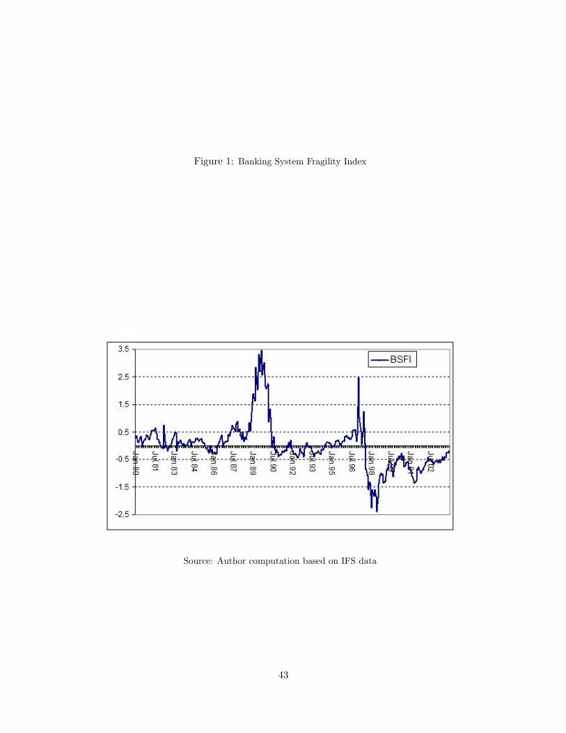
Figure 1 shows the BSFI index for Indonesia. It presents three phases: a phase

with higher index value consisting of two periods (1988-1990, and 1996-1997), a phase with

the index value around zero over two periods (1980-1987, and 1991-1996), and a phase with

lower index value for one period (1998-2003).

[INSERT FIGURE 1 HERE]

The two higher value periods are driven by different causes. The 1988-1997 period was

a consequence of the introduction of the first major package of removal of entry restrictions.

In fact, in October 1988, the government introduced a new legislation that allowed the

private sector to create and manage banks. This legislation stimulated the banking activity

through the credit channel, since newly created banks provided new loans to the private

sector, which in turn translated into new deposits. The Indonesian banking system took

approximately two years to return to the normal trend in its activities. By contrast, the

1996-1997 period was driven by an increase of credit to the private sector due to an increase

of foreign capital in the Indonesian banking system. It was also a consequence of the 1994

regulation removing the ceiling on the maximum share of investment a foreign investor can

withdraw, and also the 1996 regulation allowing mutual funds to be 100 percent foreign-

owned.

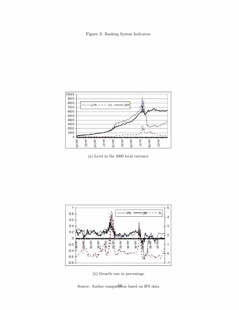
[INSERT FIGURE 2 HERE]

The two medium-value periods are periods with smooth dynamics in the banking activ-

ity. In those periods there is no important change in regulation, nor in the banking system

structure. Figure 2 (b) shows that during these periods the annual growth rate of credit to

the private sector and bank deposits are stable around 20 percent.

The lower index phase is a consequence of the Asian financial crisis, which followed the

collapse of the Thailand currency during the second half the year 1997. As we can see in

figure 2 (a) and (b), the dynamics of the three banking indicators changed dramatically

in 1997, that is a change in the level and in the trend. We guess that these three phases

characterize the states of the Indonesian banking activities during the sample period of

1980-2003.

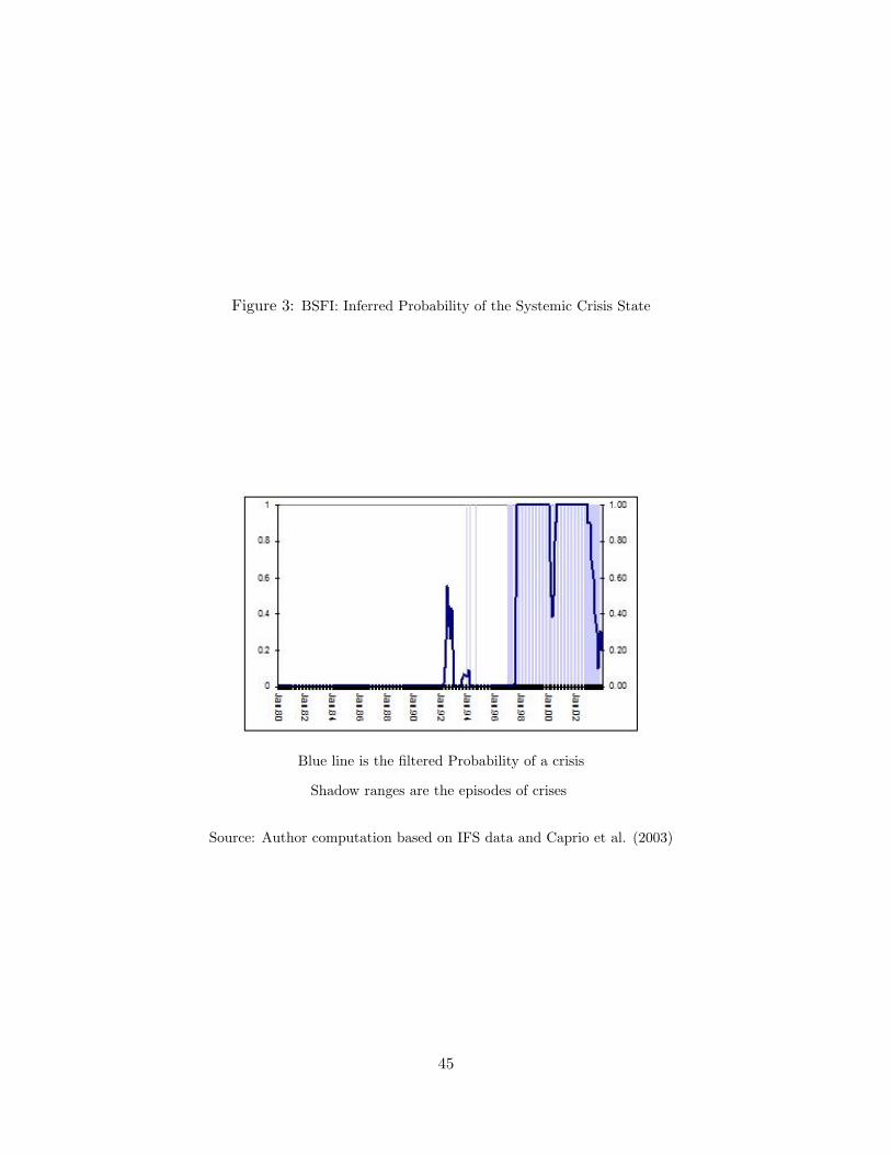
[INSERT FIGURE 3 HERE] Figure 3 compares the episodes of crises obtained with the

MSM on the BSFI index and the episodes provided by Caprio et al. (2003). The episode

of 1997-2002 matches perfectly, there is a crisis in 1992 not reported by Caprio et al.

12

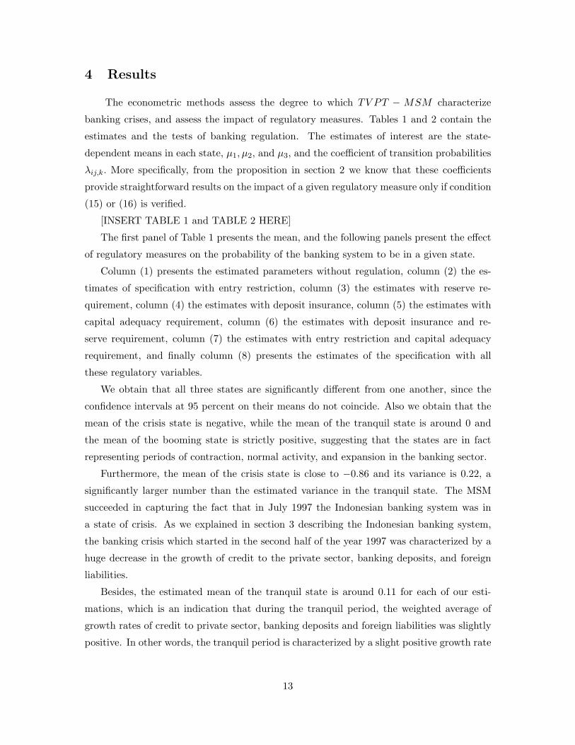
4 Results

The econometric methods assess the degree to which TV PT − MSM characterize

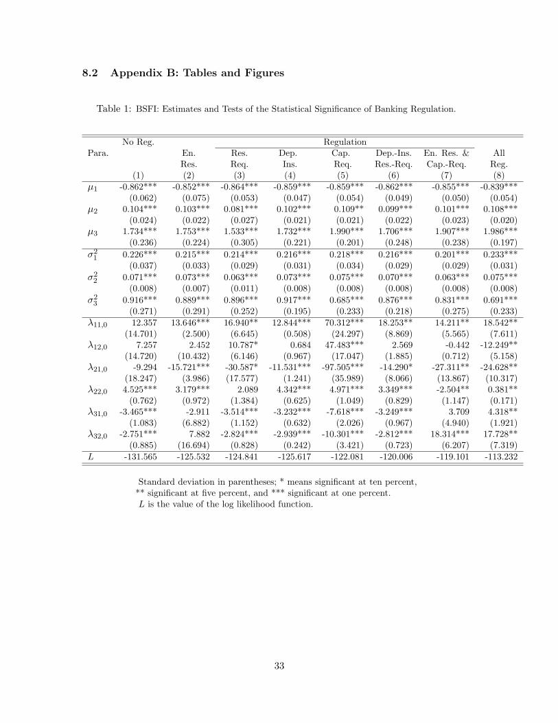
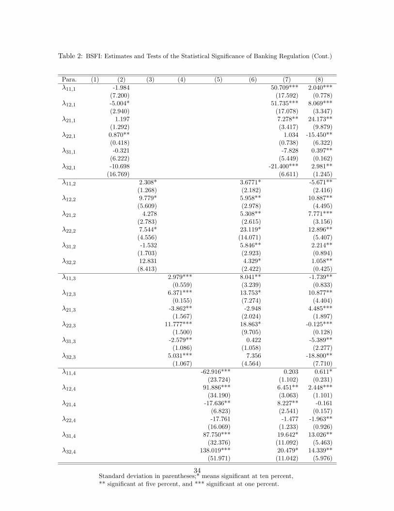
banking crises, and assess the impact of regulatory measures. Tables 1 and 2 contain the

estimates and the tests of banking regulation. The estimates of interest are the state-

dependent means in each state, µ1, µ2, and µ3, and the coefficient of transition probabilities

λij,k. More specifically, from the proposition in section 2 we know that these coefficients

provide straightforward results on the impact of a given regulatory measure only if condition

(15) or (16) is verified.

[INSERT TABLE 1 and TABLE 2 HERE]

The first panel of Table 1 presents the mean, and the following panels present the effect

of regulatory measures on the probability of the banking system to be in a given state.

Column (1) presents the estimated parameters without regulation, column (2) the es-

timates of specification with entry restriction, column (3) the estimates with reserve re-

quirement, column (4) the estimates with deposit insurance, column (5) the estimates with

capital adequacy requirement, column (6) the estimates with deposit insurance and re-

serve requirement, column (7) the estimates with entry restriction and capital adequacy

requirement, and finally column (8) presents the estimates of the specification with all

these regulatory variables.

We obtain that all three states are significantly different from one another, since the

confidence intervals at 95 percent on their means do not coincide. Also we obtain that the

mean of the crisis state is negative, while the mean of the tranquil state is around 0 and

the mean of the booming state is strictly positive, suggesting that the states are in fact

representing periods of contraction, normal activity, and expansion in the banking sector.

Furthermore, the mean of the crisis state is close to −0.86 and its variance is 0.22, a

significantly larger number than the estimated variance in the tranquil state. The MSM

succeeded in capturing the fact that in July 1997 the Indonesian banking system was in

a state of crisis. As we explained in section 3 describing the Indonesian banking system,

the banking crisis which started in the second half of the year 1997 was characterized by a

huge decrease in the growth of credit to the private sector, banking deposits, and foreign

liabilities.

Besides, the estimated mean of the tranquil state is around 0.11 for each of our esti-

mations, which is an indication that during the tranquil period, the weighted average of

growth rates of credit to private sector, banking deposits and foreign liabilities was slightly

positive. In other words, the tranquil period is characterized by a slight positive growth rate

13

in banking activity. Its estimated variance of 0.07 is lower than the variance in the other

states. This was expected as tranquil states tend to be periods of less volatility; generally,

there are periods of business as usual, i.e., no external shocks nor changes in the banking

industry.

Finally, the estimated mean of the booming state is around 1.9 with a variance of 0.7.

This value is high compared to the expected maximum value of 3 at a 99 percent confidence

level. It means also that in booming periods the weighted average of credit to the private

sector, banking deposits, and foreign liabilities grows very fast. In fact, the two periods of

fast growth of the Indonesian banking sector were characterized by sudden and very high

increases of banking deposits and credit to the private sector.

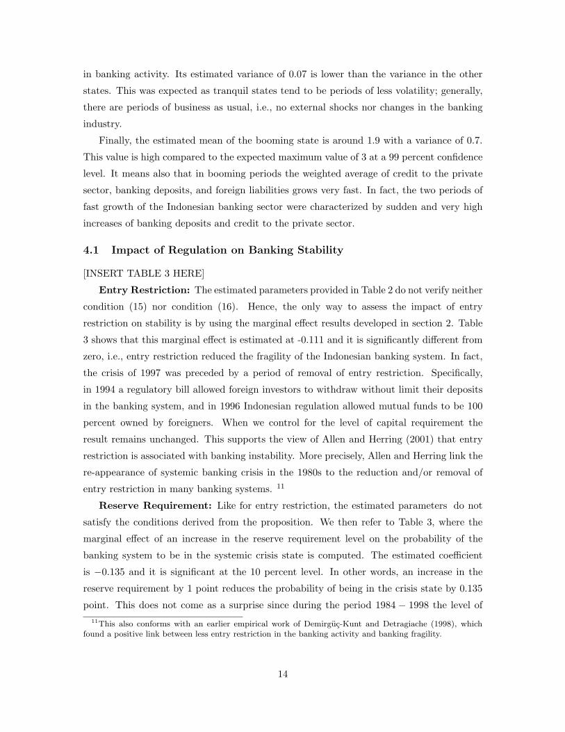
4.1 Impact of Regulation on Banking Stability

[INSERT TABLE 3 HERE]

Entry Restriction: The estimated parameters provided in Table 2 do not verify neither

condition (15) nor condition (16). Hence, the only way to assess the impact of entry

restriction on stability is by using the marginal effect results developed in section 2. Table

3 shows that this marginal effect is estimated at -0.111 and it is significantly different from

zero, i.e., entry restriction reduced the fragility of the Indonesian banking system. In fact,

the crisis of 1997 was preceded by a period of removal of entry restriction. Specifically,

in 1994 a regulatory bill allowed foreign investors to withdraw without limit their deposits

in the banking system, and in 1996 Indonesian regulation allowed mutual funds to be 100

percent owned by foreigners. When we control for the level of capital requirement the

result remains unchanged. This supports the view of Allen and Herring (2001) that entry

restriction is associated with banking instability. More precisely, Allen and Herring link the

re-appearance of systemic banking crisis in the 1980s to the reduction and/or removal of

entry restriction in many banking systems. 11

Reserve Requirement: Like for entry restriction, the estimated parameters do not

satisfy the conditions derived from the proposition. We then refer to Table 3, where the

marginal effect of an increase in the reserve requirement level on the probability of the

banking system to be in the systemic crisis state is computed. The estimated coefficient

is −0.135 and it is significant at the 10 percent level. In other words, an increase in the

reserve requirement by 1 point reduces the probability of being in the crisis state by 0.135

point. This does not come as a surprise since during the period 1984 − 1998 the level of11This also conforms with an earlier empirical work of Demirguc-Kunt and Detragiache (1998), which

found a positive link between less entry restriction in the banking activity and banking fragility.

14

the reserve requirement in Indonesia was very low, at 2 percent. It was increased in 1998

to 5 percent as the aftermath of the 1997 systemic banking crisis. It was also raised at a

time when the government was putting in place its explicit and universal deposit insurance.

This may not be a coincidence, since the deposit insurance regulation literature emphasizes

the need of reserve requirements to reduce the moral hazard problem associated with the

existence of an explicit deposit guarantee.12 It is then important to control for this. When

we control for the existence of an explicit guarantee for banking deposits, we observe that

the sign of this elasticity is different. The elasticity is now positive and equal to 0.155 and

it is significant at the one percent level. In other words, when we control for the existence

of deposit insurance, the reserve requirement is actually positively associated with banking

instability.

This second result is more appropriate. In fact, the first estimation can be viewed as

an estimation with an omitted variable, which means that the parameters estimated in this

context are biased and inconsistent. Finally, we do not worry about multicollinearity as

the coefficient of correlation between deposit insurance and reserve requirement is small

(−0.11).

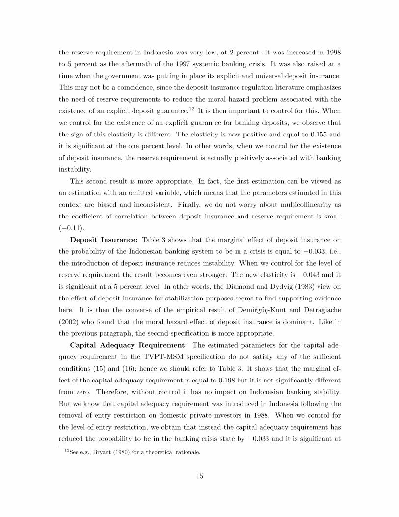
Deposit Insurance: Table 3 shows that the marginal effect of deposit insurance on

the probability of the Indonesian banking system to be in a crisis is equal to −0.033, i.e.,

the introduction of deposit insurance reduces instability. When we control for the level of

reserve requirement the result becomes even stronger. The new elasticity is −0.043 and it

is significant at a 5 percent level. In other words, the Diamond and Dydvig (1983) view on

the effect of deposit insurance for stabilization purposes seems to find supporting evidence

here. It is then the converse of the empirical result of Demirguc-Kunt and Detragiache

(2002) who found that the moral hazard effect of deposit insurance is dominant. Like in

the previous paragraph, the second specification is more appropriate.

Capital Adequacy Requirement: The estimated parameters for the capital ade-

quacy requirement in the TVPT-MSM specification do not satisfy any of the sufficient

conditions (15) and (16); hence we should refer to Table 3. It shows that the marginal ef-

fect of the capital adequacy requirement is equal to 0.198 but it is not significantly different

from zero. Therefore, without control it has no impact on Indonesian banking stability.

But we know that capital adequacy requirement was introduced in Indonesia following the

removal of entry restriction on domestic private investors in 1988. When we control for

the level of entry restriction, we obtain that instead the capital adequacy requirement has

reduced the probability to be in the banking crisis state by −0.033 and it is significant at12See e.g., Bryant (1980) for a theoretical rationale.

15

5 percent.13

There is, however, a negative correlation between entry restriction and the other reg-

ulatory measures that we have studied. This correlation is close to −0.48 for reserve re-

quirement, −0.55 for deposit insurance, and −0.67 for capital adequacy requirement. This

can be a source of multicollinearity. However, we have controlled for multicollinearity by

dropping 2.5 percent, and 5 percent of the sample data, and we have found that the re-

sult remained almost the same. Therefore, we concluded that multicollinearity was not an

important issue.

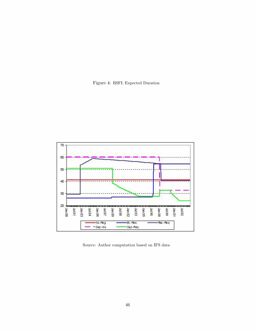
4.2 Expected Duration

Another goal of this paper is to study the expected duration of the systemic crisis state.

The three-state MSM with constant probabilities of transition shows that the expected

duration of banking crises is equal to 42 months. As we can see in Figure 4, the expected

duration is affected by banking regulations. More precisely, the presence of deposit insurance

tends to reduce crisis duration. An increase of the capital adequacy requirement tends also

to reduce crisis duration; also an increase in the reserve requirement reduces crisis duration

(see table 4). 14

[INSERT FIGURE 4 and TABLE 4 HERE]

5 Robustness

In this section, we verify the robustness of our results. First, we assess the impact of

banking regulation using another index of banking crisis, and then we verify whether we

used the appropriate number of states.

5.1 Sensitivity to the Index

In the BSFI, each type of risk is weighted equally. This can be a source of misidentifi-

cation as it tends to give each type of risk the same importance in causing banking crises.

We modify the BSFI to take into account this issue and we rename the new index as the

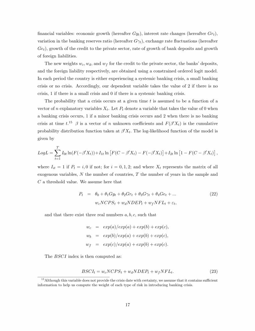
banking system crisis index (hereafter the BSCI). We use the weighting procedure of the

monetary condition index (MCI) literature (see, e.g., Duguay (1994), and Lin (1999)), but

instead of running a free regression we estimate a constrained regression. More precisely,

we assume that a banking crisis can be determined by a number of macroeconomic and13This result does not confirm the Kim and Santomero (1988), and Blum (1999) view that capital adequacy

requirement increases the risk taking behavior in the banking industry.14A policy implication which can be derived from this finding is that there is a need to design regulatory

measures that can improve the crisis duration, and not only to prevent its occurrence.

16

financial variables: economic growth (hereafter Gyt), interest rate changes (hereafter Grt),

variation in the banking reserves ratio (hereafter Gγt), exchange rate fluctuations (hereafter

Get), growth of the credit to the private sector, rate of growth of bank deposits and growth

of foreign liabilities.

The new weights wc, wd, and wf for the credit to the private sector, the banks’ deposits,

and the foreign liability respectively, are obtained using a constrained ordered logit model.

In each period the country is either experiencing a systemic banking crisis, a small banking

crisis or no crisis. Accordingly, our dependent variable takes the value of 2 if there is no

crisis, 1 if there is a small crisis and 0 if there is a systemic banking crisis.

The probability that a crisis occurs at a given time t is assumed to be a function of a

vector of n explanatory variables Xt. Let Pt denote a variable that takes the value of 0 when

a banking crisis occurs, 1 if a minor banking crisis occurs and 2 when there is no banking

crisis at time t.15 β is a vector of n unknown coefficients and F (β′Xt) is the cumulative

probability distribution function taken at β′Xt. The log-likelihood function of the model is

given by

LogL =T∑

t=1

I0t ln(F (−β′Xt))+I1t ln[F (C − β′Xt)− F (−β′Xt)

]+I2t ln

[1− F (C − β′Xt)

],

where Iit = 1 if Pt = i, 0 if not; for i = 0, 1, 2; and where Xt represents the matrix of all

exogenous variables, N the number of countries, T the number of years in the sample and

C a threshold value. We assume here that

Pt = θ0 + θ1Gyt + θ2Grt + θ3Gγt + θ4Get + ... (22)

wcNCPSt + wdNDEPt + wfNFLt + εt,

and that there exist three real numbers a, b, c, such that

wc = exp(a)/exp(a) + exp(b) + exp(c),

wb = exp(b)/exp(a) + exp(b) + exp(c),

wf = exp(c)/exp(a) + exp(b) + exp(c).

The BSCI index is then computed as:

BSCIt = wcNCPSt + wdNDEPt + wfNFLt. (23)

15Although this variable does not provide the crisis date with certainty, we assume that it contains sufficientinformation to help us compute the weight of each type of risk in introducing banking crisis.

17

To obtain the index with the Indonesian data, we complete our previous dataset so as

to be able to compute Gy, Gr,Gγ and Ge.16 The variable for banking crises is obtained

from Caprio et al. (2003). For Indonesia the estimate of the reduced form model presented

in (22) is given by:

Pt = −0.06 + 6.58Gyt−1.50Grt+0.44Gγt−4.78Get+...

(−0.20) (8.45) (−4.61) (1.11) (−1.77)...

0.8049NCPSt +0.195NDEP t +[7.04E − 8]NFLt

(2.02) (1.98) (0.77)

The student t−statistics are in parentheses. We obtain from the above estimation that

wc = 0.8049, wd = 0.195, and wf = 7.04E−08. We observe that the weight for the credit to

the private sector is greater than the weight of bank deposits. More importantly, the weight

for foreign liability is practically zero. This may be due to the fact that the Indonesian

banking crisis was introduced by non-performing loans. In fact, in mid-1997 most domestic

firms could not service their liabilities to international and domestic banks.17 This later

translated into a severe liquidity problem arising from increased burdens of firms servicing

external debts, and was exacerbated by mass withdrawal of deposits.

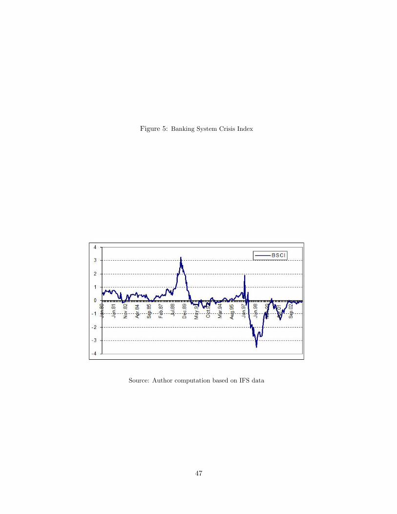
[INSERT FIGURE 5 HERE]

Figure 5 presents the new index. We observe that the graph of the BSCI is similar to

the graph of the BSFI. We can then guess that we should obtain the same results.

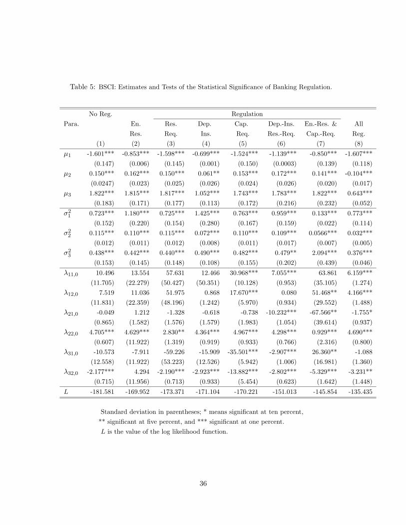
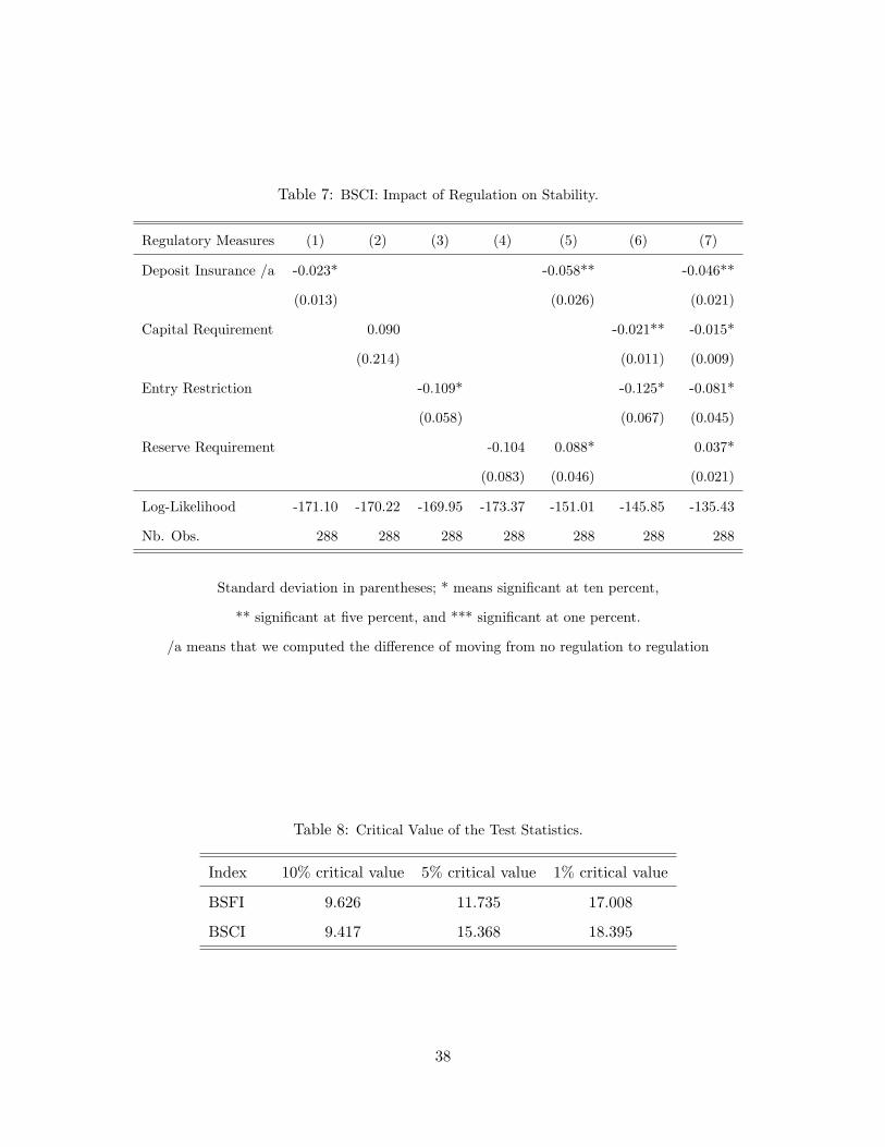
[INSERT TABLE 5, TABLE 6 and TABLE 7 HERE]

Table 5 and Table 6 provide the raw parameters while Table 7 provides the marginal

effect of each regulatory measure on the probability of the banking system going into crisis.

We observe that the results are fundamentally the same for each type of regulation. The

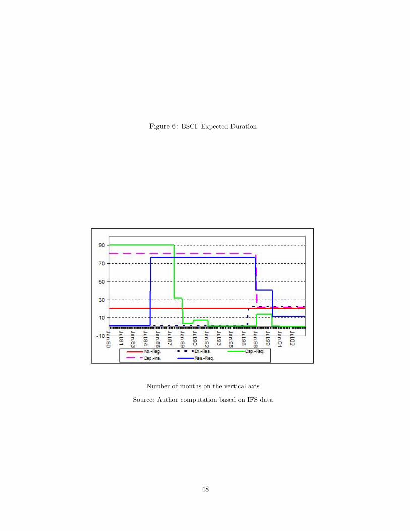
results differ slightly on the crisis duration. In fact, the expected crisis duration is 42 months

for the BSFI index while it is 21 months for the BSCI; but the impact of each type of

regulation on the expected duration is exactly the same (see figure 6).

[INSERT FIGURE 6 HERE]16To compute Ge we use the data on exchange rate available from IFS’s line AF . To compute Gr we

use the nominal interest rate from IFS’s line 60B. To compute Gy we use the information on the real GDPgrowth available in the World Development Indicator (WDI) 2006. To compute Gγ we use the demanddeposits from (IFS line 24) , the time and saving deposits (IFS line 25), the foreign liabilities (IFS line 26C)of deposit money banks and the credit from monetary authorities (IFS line 26G).

17See e.g., Enoch et al. (2001) for a better description of the state of the Indonesian banking systemduring that period.

18

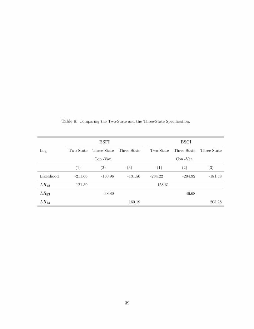
5.2 Sensitivity to the MSM Specification

In this subsection we verify that the three-state specification with different variances

for each state is the appropriate model. We compare this specification with the two-state

specification and with the three-state specification but with constant variance. Our choice

of model is based on the likelihood ratio (LR) test. The distribution of the LR statistic

between constant variance and state-varying variance is the standard χ2. But it is no longer

the case between the two-state and the three-state specification.18 This is due to the fact

that under the null of a Q − 1−state model, the parameters describing the Qth state are

unidentified. To solve this problem we follow Coe (2002) in performing a Monte Carlo

experiment to generate empirical critical values for the sample test statistic. For each

index, we first run a two-state MSM . We then use its estimated parameters to generate an

artificial index. We use this index to estimate both the two-state model and the three-state

model by the maximum likelihood method. Finally, we calculate the likelihood ratio test

statistic. Let us denote by MLi the maximum likelihood of the i−state model. The test

statistic is given by

LR2 = −2 [Log(ML2)− Log(ML3)] . (24)

We generate this index randomly one thousand times, and follow this procedure the same

number of times to obtain the empirical distribution of the test statistic. In Table 9 we

report the critical values of these test statistics.

[INSERT TABLE 8 and 9 HERE]

Let’s now implement the test. The test statistics (obtained in Table 9) show that the

value of the likelihood ratio test is above the critical one percent values presented in Table

8. It follows that on the basis of this test the three-state specification should be chosen

instead of the two-state. The same result holds with the BSCI index.

6 Assessing the Selection and the Simultaneity Bias

We now assess the selection and the Simultaneity bias in the existing work.

6.1 Assessment of the Simultaneity Bias

In this subsection we want to see if the results obtained so far about the link between

the type of regulation and banking stability would have been obtained by implementing a

simple three-state MSM model, and use its filtered probabilities to estimate with a simple18In fact, from Garcia (1998) we know that the LR test statistic in this context does not possess the

standard distribution.

19

OLS regression the effect of each regulation on the stability of the banking system. We will

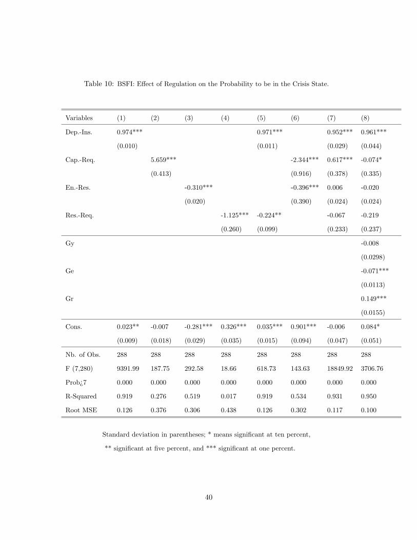
refer to this method as the MSM −OLS regression. 19 In Table 10, we report the results

obtained from the MSM −OLS regression.

[INSERT TABLE 10 HERE]

Deposit insurance appears to have a positive and significant effect on the probability of

the banking system to be in the systemic crisis period. When we control for other regulatory

measures, this effect is equal to 0.82; with macroeconomic variables the new number is 0.81.

The effect of a reserve requirement, when we control for the entire set of major regulatory

variables, is equal to 0.95 and is 0.81 when we add key macroeconomic variables. The

capital adequacy requirement has a negative and significant effect on the probability of the

banking system being in the crisis state. In fact, when we control for the other regulatory

variables, this effect is equal to −0.78; while it is equal to −0.32 when we control for other

macroeconomic variables. Finally, the effect of entry restriction is significant and negative

even when we control for other regulatory measures.

Let us now assess the difference between the two methods. Deposit insurance increases

the probability of being in a crisis in the MSM −OLS regression but not in the TV PT −MSM . This difference can be explained by the fact that deposit insurance was put in place

in 1998, a crisis year. Therefore, the MSM −OLS perceives a positive correlation between

its presence and the occurrence of the banking crisis even though the crisis preceded it. The

MSM −OLS shows a higher impact of the capital adequacy requirement for stabilization

purposes than the TV PT −MSM . A rationale behind this is that just after the beginning

of the banking crisis in 1997, the Indonesian government reduced the rate of its capital

adequacy requirement and then started to increase it slowly. Hence, the MSM − OLS

perceives a stronger link between the reduction of the capital adequacy requirement and

the presence of banking crises. The result on entry restriction is not too different. In the

TV PT −MSM, reserve requirements have a less positive impact on banking stability than

in the MSM −OLS. More generally, the marginal effects produced by the TV PT −MSM

tend to be less important in magnitude.

6.2 Assessment of the Selection Bias

We now assess the selection bias in the existing work. For this purpose we compare

our estimates to estimates obtained with the logit method used in the previous literature.

Since the previous works were conducted mostly with cross-country data, we first develop

another discrete regression model to have specific coefficients on Indonesia.19The MSM −OLS is very tractable and allows the introduction of many control variables.

20

6.2.1 The Ordered Logit Model (OLM)

We estimate the probability of a banking crisis using an ordered logit model. In each

period the country is either experiencing a systemic banking crisis, a small banking crisis

or no crisis. Accordingly, our dependent variable takes the value 2 if there is no crisis, 1 if

there is a small crisis and 0 if there is a systemic banking crisis.

The probability that a crisis occurs at a given time t is assumed to be a function of a

vector of n explanatory variables Xt. Let Pt denote a variable that takes the value of 0

when a banking crisis occurs, 1 when a minor banking crisis occurs and 2 when no banking

crisis occurs at time t. β is a vector of n unknown coefficients and F (β′Xt) is the cumulative

probability distribution function taken at β′Xt. The log-likelihood function of the model is

given by

LogL =T∑

t=1

I0t ln(F (−β′Xt))+I1t ln[F (C − β′Xt)− F (−β′Xt)

]+I2t ln

[1− F (C − β′Xt)

],

where Iit = 1 if Pt = i, 0 if not; for i = 0, 1, 2; and where Xt represents the matrix of all

exogenous variables, N the number of countries, T the number of years in the sample and

C a threshold value. We then use the estimated parameters to compute the marginal effect

of each regulatory measure for the probability of the banking system being in a systemic

crisis.

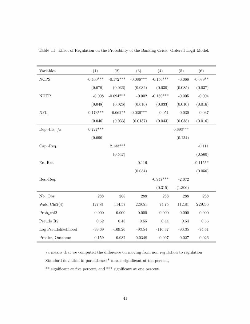
[INSERT TABLE 11 HERE]

In Table 11 we report the results using the ordered logit model. The banking crisis

variable is given by Caprio et al. (2003). We observe that deposit insurance appears to

have a positive and significant marginal effect of the probability for the banking system being

in the systemic crisis period. When we control for other regulatory measures, this marginal

effect is equal to 0.69. The reserve requirement has no marginal significant effect on the

probability of the banking system being in the systemic crisis period. The marginal effect

of the capital adequacy requirement is not significantly different from zero when we control

for other regulatory measures. Finally, the marginal effect of entry restriction is significant

and negative even when we control for the existence of capital adequacy requirement.

6.2.2 Results of the Previous Work

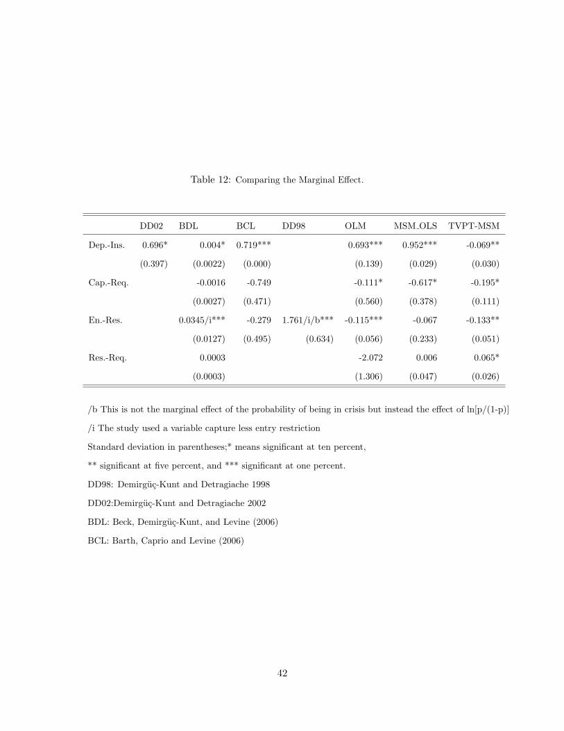
[INSERT TABLE 12 HERE]

Table 12 shows that previous works link deposit insurance to instability. We found that

in the Indonesian case if we used the OLM or the MSM − OLS we still have the same

result. But the result is different if we use the TV PT −MSM . In the later case deposit

21

insurance improves banking stability. Hence, the selection bias is not the only issue to deal

with. This suggests that the simultaneity bias due to the adoption of full deposit insurance

during the crisis is better taken into account by the TV PT − MSM than by the other

models.

Previous studies found a non-significant link between the capital requirement and bank-

ing fragility.20 But, with Indonesia, we obtain a significant negative link at 10 percent.

When we used the OLM, the link is also significant and negative, but less than the coef-

ficient of the event-based method. We can then infer a negative selection bias. But even

here the magnitude of the TV PT − MSM coefficient is significantly different from the

MSM − OLS coefficient. We guess that this is due to the simultaneity bias. In fact, the

Indonesian government reduced the level of the capital adequacy requirement during the

crisis and started to increase it as the situation was improving. The TV PT − MSM is

more able to take this feature into account.

Entry restriction has been linked to stability by the previous studies. We obtain the

same result here and no significant bias.

Concerning the reserve requirement, studies using event-based data found mixed results

on the link between the reserve requirement and instability. This is not the case with the

MSM − OLS. Instead, we found a positive and significant link between higher reserve

requirement and instability. Therefore, the selection bias is positive. As in the previous

case we found that the simultaneity bias is also important.

7 Conclusion

The first goal of this research was to provide an estimation strategy that was less

subject to selection bias as well as simultaneity bias and to use it to assess empirically

the effect of banking regulations on the banking system stability. The second goal was to

assess the effect of each type of regulation on crisis duration. To this end, we developed

a three-state Markov-switching regression model. Specifically, we introduced four major

regulations (entry restriction, deposit insurance, reserve requirement, and capital adequacy

requirement) as explanatory variables of the probability of transition of one state to another

in order to assess the effect of these regulations on the occurrence and the duration of

systemic banking crises.

Given that the time-varying probability of transition TVPT-MSM does not provide a20For example, Barth et al. (2004) found a negative coefficient for the capital adequacy requirement which

varied from −1.201 to −1.026 in some of their specifications depending on whether they were significant ornot; while Beck et al. (2006) found a non significant term for the link between capital adequacy requirementand banking crisis.

22

straightforward measure of the marginal effect of exogenous variables on the probability of

the system to be in a given state, we derived the marginal effect of each exogenous variable

on the probability of the system being in a given state. This is our theoretical contribution

to the MSM literature. We then applied our strategy to the Indonesian banking system,

which has suffered from systemic banking crises during the last two decades and where there

has been some dynamics on the regulatory measures during the same period.

We found that: (i) entry restriction reduces crisis duration and the probability of being

in the crisis state. This result is consistent with other results available in the banking crisis

literature linking banking crises and an easing of entry restrictions; (ii) reserve require-

ments increase banking fragility; but this result is obtained only when we take into account

the existence of deposit insurance. At the same time reserve requirements tend to reduce

banking crisis duration; (iii) the deposit insurance increases the stability of the Indonesian

banking system and reduces the banking crisis duration. This result is different from the

Demirguc-Kunt and Detragiache (2002) result about the link between the existence of ex-

plicit deposit insurance and banking fragility, and it raises a flag about the importance of

the simultaneity bias in this type of studies; (iv) the capital adequacy requirement improves

stability and reduces the expected duration of a banking crisis; this result is obtained when

we control for the level of entry restrictions.

We have also provided an idea of the selection and simultaneity bias present in the

previous literature. We found a negative simultaneity bias for deposit insurance due to the

fact that this policy was adopted and implemented in 1998 during a crisis period. Therefore,

any estimation technique that does not take this simultaneity aspect into account will tend

to link insurance and instability. When this is taken into account we move from 0.7 to -0.1.

We also found a negative selection bias for capital adequacy requirement, i.e. when we use

MSM the effect of this regulation on the banking sector stability is more important; the

coefficient moves from -0.1 to -0.6. A rationale for this is the fact that the 1994 episode is

taken into account.

It then appears that the TV PT −MSM can improve our understanding of the impact

of regulation on banking activities by allowing us to work on a given country, taking into

account the selection bias as well as the simultaneity bias. In fact, in the TV PT −MSM,

the states of nature and the effect of regulation on the occurrence of each state are jointly

estimated. In other words, the TV PT −MSM is a type of a simultaneous equation model.

Finally, it helps to provide an assessment of the impact of regulatory measures on the ex-

pected duration of crises. However, it presents an important limitation. It is less tractable

when the number of exogenous variables explaining the probability of transition is impor-

23

tant. In fact, in a three-state TV PT − MSM the introduction of an additional variable

leads to the estimation of six new parameters. This makes the convergence of the maximum

likelihood estimation technique more difficult to achieve and complicates the estimation pro-

cess.

24

References

[1] Abdullah, Burhanuddin, and Santoso Wimboh. 2001. ”The Indonesian Banking Indus-

try: Competition, Consolidation, and Systemeic Stability ”, Bank for International

Settlement, Paper No.4.

[2] Allen, Franklin, and Douglas Gale. 2003. ”Capital Adequacy regulation: In search of

a Rationale. ” In Richard Arnott, Bruce Greenwald, Ravi Kanbur and Barry Nale-

buff., (Eds), Economics for an Imperfect World: Essays in Honor of Joseph Stiglitz.

Cambridge, MA: MIT Press.

[3] Allen, Franklin, and Douglas Gale. 2004. ”Financial Intermediaries and Markets, ”

Econometrica, 72: 1023-1061.

[4] Allen, Franklin, and Richard Herring. 2001. ”Banking Regulation Versus Securities

Market Regulations, ” Center for Financial Institutions, Working Paper 01-29, Whar-

ton School Center for Financial Institutions, University of Pennsylvania

[5] Barth, James R., Gerard Caprio, and Ross Levine. 2004. ”Bank Supervision and Reg-

ulation: What Works Best?”, Journal of Financial Intermediation Vol. 13, No. 2.

[6] Batunanggar, Sukarela. 2002. ”Indonesia’s Banking Crisis Resolution :Lessons and The

Way Forward.” The Centre for Central Banking Studies (CCBS), Bank of England

[7] Beck, Thorsten, Asli, Demirguc-Kunt, and Ross Levine. 2006. ”Bank Concentration,

Competition, and Crises: First Results ”, Journal of Banking and Finance, 30: 1581-

1603.

[8] Blum, Jurg. 1999. ”Do Capital Adequacy Requirements Reduce Risks in Banking?”

Journal of Banking and Finance, 23: 755-771.

[9] Bryant, John. 1980. ”A Model of Reserves, Bank Runs, and Deposit Insurance, ”

Journal of Banking and Finance, 4:335-344.

[10] Caprio, Gerard, Daniel Klingebiel, Luc, Laeven, and G. Noguera.2003. Banking Crises

Database ; www1.worldbank.org/finance/html/database sfd.html.

[11] Caprio, Gerard, and Daniela Klingebiel. 2002. ”Episodes of Systematic and Borderline

Financial Crises, ” In Daniela Klingebiel and Luc Laeven (Eds.), Managing the Real

and Fiscal Effects of Banking Crises, World Bank Discussion Paper No. 428.

25

[12] Caprio, Gerard, and Daniela Klingebiel. 1996. “Bank Insolvency: Bad Luck, Bad Pol-

icy, or Bad Banking?” Annual World Bank Conference on Development Economics

1996.

[13] Coe, Patrick J. 2002. ”Financial Crisis and the Great Depression: A Regime Switching

Approach”, Journal of Money, Credit, and Banking, 34 (1): 76-93.

[14] Demirguc-Kunt, Asli, and Enrica Detragiache. 2002. ”Does Deposit Insurance Increase

Banking System Stability? An Empirical Investigation”, Journal of Monetary Eco-

nomics, 49: 1373-406.

[15] Demirguc-Kunt, Asli, and Enrica Detragiache. 1998. ”Financial Liberalization and Fi-

nancial Fragility” The World Bank Policy Research Working Paper, No.1917.

[16] Demirguc-Kunt, Asli, Edward J. Kane, and Luc Laeven. 2006. ”Determinants of

Deposit-Insurance Adoption and Design,” The World Bank Policy Research Working

Paper 3849.

[17] Demirguc-Kunt, Asli, Enrica Detragiache, and Poonam Gupta. 2006. ”Inside the crisis:

An empirical analysis of Banking Systems in Distress”, Journal of International Money

and Finance, 25: 702-718.

[18] Diamond, Douglas W., and Philip H. Dybvig. 1983. ”Bank Runs, Deposit Insurance,

and Liquidity, ” Journal of Political Economy, 91 (3): 401–419.

[19] Diebold, Francis X., Joon-Haeng Lee, and Gretchan C. Weinbach. 1994. ”Regime

Switching with time-varying transition probabilities, ” in Business Cycles, Indica-

tors, and Forecasting, Eds. J.H. Stock and M.W. Watson, Chicago: The University

of Chicago Press, pp.255-280.

[20] Duguay, Pierre. 1994. ”Empirical Evidence on the Strength of Monetary Transmission

Mechanism in Canada, ” Journal of Monetary Economics, 33.

[21] Eichengreen, Barry, Andrew K. Rose, and Charles Wyplosz. 1996. “Contagious Cur-

rency Crises,” NBER Working Papers No. 5681.

[22] Eichengreen, Barry, Andrew K. Rose , and Charles Wyplosz. 1995. “Exchange Market

Mayhem: The Antecedents and Aftermath of Speculative Attacks,” Economic Policy,

21: 249-296.

26

[23] Eichengreen, Barry, Andrew K. Rose, and Charles Wyplosz. 1994. ”Speculative Attacks

on Pegged Exchange Rate: An Empirical Exploration with special Reference to the

European Monetary System,” NBER Working Papers No. 4898.

[24] Enoch, Charles, Barbara Baldwin, Olivier Frecault, and Arto Kovanen. 2001. ”Indone-

sia: Anatomy of a Banking Crisis Two years of Living Dangerously 1997-99 ” The IMF

Working Paper No. WP/01/52, P.64.

[25] Filardo, Andrew J. 1994. ”Business-Cycle Phases and Their Transitional Dynamics”;

Journal of Business and Economic Statistics, 12 (3): 299-308.

[26] Filardo, Andrew J., Stephen F. Gordon. 1998. “Business Cycle Durations,” Journal of

Econometrics, 85 (1): 99–123.

[27] Garcia, Rene. 1998. “Asymptotic Null Distribution of the Likelihood Ratio Test in

Markov Switching Models”, International Economic Review, 39 (3): 763-788.

[28] Garcia, Rene, and Pierre Perron. 1996. ”An Analysis of Real Interest Under Regime

Shift.” Review of Economics and Statistics, No. 78.

[29] Hein, Scott E., and Jonathan D. Stewart. 2002. ”Reserve Requirements: A Modern

Perspective, ” Federal Reserve Bank of Atlanta Economic Review, 4th Quarter 2002.

[30] Ho, Tai-kuang. 2004. ”How Useful Are Regime-Switching Models In Banking Crises

Identification? ”, Econometric Society Far Eastern Meeting No. 764.

[31] Hawkins, John, and Marc Klau. 2000. “Measuring Potential Vulnerabilities in Emerging

Market Economies,” BIS Working Paper No 91.

[32] Kibritcioglu, Aykut. 2002. “Excessive Risk-Taking, Banking Sector Fragility, and Bank-

ing Crises,” Office of Research Working Paper Number 02-0114, University of Illinois

at Urbana-Champaign.

[33] Kim, Chang-Jin, and Charles R. Nelson. 1999. ”State-Space Models with Regime

Swithing ”, The MIT Press.

[34] Kim, Daesik, and Anthony M. Santomero. 1988. ”Risk in Banking and Capital Regu-

lation,” Journal of Finance 43: 1219-1233.

[35] Lin, Jin-Lung. 1999. ”Monetary Conditions Index in Taiwan,” Academia Economic

Papers, 2000 (27): 459-479

27

[36] Matutes, Carmen, and Xavier Vives. 1996. ”Competition for Deposit, Fragility, and

Insurance.” Journal of Financial Intermediation 5 (2): 184–216.

[37] Maddala, G. S. 1986. ”Disequilibrium, Self-Selection, and Switching Models”, in Hand-

book of Econometrics, Volume 3, Edited by Z. Griliches and M. D. Intriligator.

[38] Morrison, Alan D. and Lucy White. 2005. ”Crises and Capital Requirements in Bank-

ing,” American Economic Review, 95, 5.

[39] Van’t Dack, Jozef. 1999. ”Implementing Monetary Policy in Emerging Market

Economies: An Overview of Issues ” in Bank for International Settlements Policy

Papers No.5.

[40] Von Hagen, Jurgen, and Tai-kuang Ho. 2007. “MoneyMarket Pressure and the Deter-

minants of Banking Crises,” Journal of Money, Credit and Banking, 39 (5): 1037 -

1066.

28

8 Appendix

8.1 Appendix A

Application of the Kim and Nelson Method on the the TVPT-MSM

Let us set ψt = {ψt−1, yt, Zt}.

Step 1. We consider the joint density of yt and the unobserved st variable, which is the

product of the conditional and marginal densities: f(yt, st|ψt−1) = f(yt|st, ψt−1)f(st|ψt−1).

Step 2. To obtain the marginal density of yt, we integrate the st variable out of the above

joint density by summing over all possible values of st:

f(yt|ψt−1) =3∑

st=1

f(yt, st|ψt−1)

=3∑

st=1

f(yt|st, ψt−1)f(st|ψt−1)

=3∑

i=1

f(yt|st = i, ψt−1) Pr(st = i|ψt−1)

The log likelihood function is then given by

lnL =T∑

t=0

ln

{3∑

i=1

f(yt|st = i, ψt−1) Pr(st = i|ψt−1)

}. (25)

The marginal density given above can be interpreted as a weighted average of the

conditional densities given st = 1, st = 2, and st = 3, respectively.

We adopt the following filter for the calculation of the weighting terms :

Step 1. Given Pr[st−1 = i|ψt−1], i = 1, 2, 3, at the beginning of time t or the t − th

iteration, the weighting terms Pr[st = j|ψt−1], j = 1, 2, 3 are calculated as

Pr[st = j|ψt−1] =3∑

i=1

Pr[st = j, st−1 = i|ψt−1]

=3∑

i=1

Pr[st = j|st−1 = i, Zt−1]Pr[st−1 = i|ψt−1],

where Pr[st = j|st−1 = i, Zt−1], i = 1, 2, 3, j = 1, 2, 3 are the transition probabilities.

29

Step 2. Once yt is observed at the end on time t, or at the end of the t− th iteration, we

update the probability term as follows:

Pr[st = j|ψt] = Pr[st = j|yt, ψt−1, yt, Zt]

=f(st = j, yt|ψt−1, Zt)

f(yt|ψt−1, Zt)

=f(yt|st = j, ψt−1, Zt) Pr[st = j|ψt−1, Zt]∑3i=1 f(yt|st = i, ψt−1, Zt) Pr[st = i|ψt−1, Zt]

.

The above two steps may be iterated to get Pr[st = j|ψt], t = 1, 2, ..., T . To start the

above filter at time t = 1, however, we need Pr[s0|ψ0]. We can employ the method of

Kim and Nelson to obtain the steady-state or unconditional probabilities

π =

Pr[s0 = 1|ψ0]Pr[s0 = 2|ψ0]Pr[s0 = 3|ψ0]

of st to start with. Where π is the last column of the matrix (A′A)−1A′ with

A =

1− p11,0 −p21,0 −p31,0

−p12,0 1− p22,0 −p32,0

−p13,0 −p23,0 1− p33,0

1 1 1

By now, it is clear that the log likelihood function in (25), is a function of µ1, µ2, µ3, σ21, σ

22, σ

23, {λij,k}

i = 1, 2, 3; j = 1, 2; k = 0, 1, ..., N.

Proof of the Lemma Proof. Let zlt be a time series variable. Let us set

g(λij) = exp(λij,0 +N∑

k=1

λij,kZkt). (26)

With this notation for i = 1, 2, 3;

pij,t =g(λij)

1 + g(λi1) + g(λi2)

for j = 1, 2; and

pi3,t =1

1 + g(λi1) + g(λi2). (27)

If zlt is a continuous variable, its marginal effect on pij,t can be computed as:

∂pij,t

∂zlt=

gl(λij) [1 + g(λi1) + g(λi2)]− g(λi1) [gl(λi1) + gl(λi2)](1 + g(λi1) + g(λi2))

2 (28)

30

Besides, direct derivation of (26) in respect with zlt yields,

gl(λij) = λij,lg(λij). (29)

Substituting (29) in (28) yields

∂pij,t

∂zlt=

λij,lg(λij) [1 + g(λi1) + g(λi2)]− g(λi1) [λi1,lg(λi1) + λi2,lgl(λi2)](1 + g(λi1) + g(λi2))

2 (30)

Developing and regrouping the right hand side of equation (30) gives

∂pij,t

∂zlt=

g(λij) [λij,l + (λij,l − λi1,l) g(λi1) + (λij,l − λi2,l) g(λi2)][1 + g(λi1) + g(λi2)]

2

Let us now compute ∂pi3,t

∂zltfor i = 1, 2, 3. A direct differentiation of (27) yields

∂pi3,t

∂zlt=

− [gl(λi1) + gl(λi2)](1 + g(λi1) + g(λi2))

2 . (31)

Substituting (29) in (31) yields

∂pi3,t

∂zlt=− [λi1,lg(λi1) + λi2,lg(λi2)]

(1 + g(λi1) + g(λi2))2 .

For dummy variable taking the value 1 or 0, the marginal effect is obtained by com-

puting pij,t = [pij,t(z−lt, 1)− pij,t(z−lt, 0)] ; where z−lt is the matrix Zt without zlt.

Proof of the Proposition Proof. We know that πt = Ptπt−1, and since

πt ≡

Pr(st = 1)Pr(st = 2)Pr(st = 3)

,

it follows that we can rewrite it as

Pr(st = 1)Pr(st = 2)Pr(st = 3)

=

p11,t p21,t p31,t

p12,t p22,t p32,t

p13,t p23,t p33,t

Pr(st−1 = 1)Pr(st−1 = 2)Pr(st−1 = 3)

. (32)

This implies that

Pr(st = 1) = p11,tPr(st−1 = 1) + p21,tPr(st−1 = 2) + p31,tPr(st−1 = 3) (33)

Pr(st = 2) = p12,tPr(st−1 = 1) + p22,tPr(st−1 = 2) + p32,tPr(st−1 = 3) (34)

Pr(st = 3) = p13,tPr(st−1 = 1) + p23,tPr(st−1 = 2) + p33,tPr(st−1 = 3). (35)

They can be regrouped in the following general form

Pr(st = j) =3∑

i=1

pij,tPr(st−1 = i).

31

It is obvious that Pr(st−1 = i) is not a function of zlt. Hence, if zlt is a continuous

variable∂ Pr(st = j)

∂zlt=

3∑

i=1

(∂pij,t

∂zlt

)Pr(st−1 = i). (36)

Substituting (10) or (11) in equation (36) gives

∂ Pr(st = j)∂zlt

=3∑

i=1

(g(λij) [λij,l + (λij,l − λi1,l) g(λi1) + (λij,l − λi2,l) g(λi2)]

[1 + g(λi1) + g(λi2)]2

)Pr(st−1 = i)

for j= 1 , 2 ; and

∂ Pr(st = 3)∂zlt

=3∑

i=1

(− [λi1,lg(λi1) + λi2,lg(λi2)][1 + g(λi1) + g(λi2)]

2

)Pr(st−1 = i).

More precisely,

∂ Pr(st = 1)∂zlt

=3∑

i=1

(g(λ1j) [λ1j,l + (λi1,l − λi2,l) g(λi2)]

[1 + g(λi1) + g(λi2)]2

)Pr(st−1 = i).

And if zlt is a dummy variable, its marginal effect on the probability of being in a

given state j is given by

∆l [Pr(st = j)] =3∑

i=1

∆lpij,t [Pr(st−1 = i)] . (37)

More precisely,

∆l [Pr(st = 1)] =3∑

i=1

[pi1,t(z−lt, 1)− pi1,t(z−lt, 0)] [Pr(st−1 = i)] .

32

8.2 Appendix B: Tables and Figures

Table 1: BSFI: Estimates and Tests of the Statistical Significance of Banking Regulation.

No Reg. RegulationPara. En. Res. Dep. Cap. Dep.-Ins. En. Res. & All

Res. Req. Ins. Req. Res.-Req. Cap.-Req. Reg.(1) (2) (3) (4) (5) (6) (7) (8)

µ1 -0.862*** -0.852*** -0.864*** -0.859*** -0.859*** -0.862*** -0.855*** -0.839***(0.062) (0.075) (0.053) (0.047) (0.054) (0.049) (0.050) (0.054)

µ2 0.104*** 0.103*** 0.081*** 0.102*** 0.109** 0.099*** 0.101*** 0.108***(0.024) (0.022) (0.027) (0.021) (0.021) (0.022) (0.023) (0.020)

µ3 1.734*** 1.753*** 1.533*** 1.732*** 1.990*** 1.706*** 1.907*** 1.986***(0.236) (0.224) (0.305) (0.221) (0.201) (0.248) (0.238) (0.197)

σ21 0.226*** 0.215*** 0.214*** 0.216*** 0.218*** 0.216*** 0.201*** 0.233***

(0.037) (0.033) (0.029) (0.031) (0.034) (0.029) (0.029) (0.031)σ2

2 0.071*** 0.073*** 0.063*** 0.073*** 0.075*** 0.070*** 0.063*** 0.075***(0.008) (0.007) (0.011) (0.008) (0.008) (0.008) (0.008) (0.008)

σ23 0.916*** 0.889*** 0.896*** 0.917*** 0.685*** 0.876*** 0.831*** 0.691***

(0.271) (0.291) (0.252) (0.195) (0.233) (0.218) (0.275) (0.233)λ11,0 12.357 13.646*** 16.940** 12.844*** 70.312*** 18.253** 14.211** 18.542**

(14.701) (2.500) (6.645) (0.508) (24.297) (8.869) (5.565) (7.611)λ12,0 7.257 2.452 10.787* 0.684 47.483*** 2.569 -0.442 -12.249**

(14.720) (10.432) (6.146) (0.967) (17.047) (1.885) (0.712) (5.158)λ21,0 -9.294 -15.721*** -30.587* -11.531*** -97.505*** -14.290* -27.311** -24.628**

(18.247) (3.986) (17.577) (1.241) (35.989) (8.066) (13.867) (10.317)λ22,0 4.525*** 3.179*** 2.089 4.342*** 4.971*** 3.349*** -2.504** 0.381**

(0.762) (0.972) (1.384) (0.625) (1.049) (0.829) (1.147) (0.171)λ31,0 -3.465*** -2.911 -3.514*** -3.232*** -7.618*** -3.249*** 3.709 4.318**

(1.083) (6.882) (1.152) (0.632) (2.026) (0.967) (4.940) (1.921)λ32,0 -2.751*** 7.882 -2.824*** -2.939*** -10.301*** -2.812*** 18.314*** 17.728**

(0.885) (16.694) (0.828) (0.242) (3.421) (0.723) (6.207) (7.319)L -131.565 -125.532 -124.841 -125.617 -122.081 -120.006 -119.101 -113.232

Standard deviation in parentheses; * means significant at ten percent,** significant at five percent, and *** significant at one percent.L is the value of the log likelihood function.

33

Table 2: BSFI: Estimates and Tests of the Statistical Significance of Banking Regulation (Cont.)

Para. (1) (2) (3) (4) (5) (6) (7) (8)λ11,1 -1.984 50.709*** 2.040***

(7.200) (17.592) (0.778)λ12,1 -5.004* 51.735*** 8.069***

(2.940) (17.078) (3.347)λ21,1 1.197 7.278** 24.173**

(1.292) (3.417) (9.879)λ22,1 0.870** 1.034 -15.450**

(0.418) (0.738) (6.322)λ31,1 -0.321 -7.828 0.397**

(6.222) (5.449) (0.162)λ32,1 -10.698 -21.400*** 2.981**

(16.769) (6.611) (1.245)λ11,2 2.308* 3.6771* -5.671**

(1.268) (2.182) (2.416)λ12,2 9.779* 5.958** 10.887**

(5.609) (2.978) (4.495)λ21,2 4.278 5.308** 7.771***

(2.783) (2.615) (3.156)λ22,2 7.544* 23.119* 12.896**

(4.556) (14.071) (5.407)λ31,2 -1.532 5.846** 2.214**

(1.703) (2.923) (0.894)λ32,2 12.831 4.329* 1.058**

(8.413) (2.422) (0.425)λ11,3 2.979*** 8.041** -1.739**

(0.559) (3.239) (0.833)λ12,3 6.371*** 13.753* 10.877**

(0.155) (7.274) (4.404)λ21,3 -3.862** -2.948 4.485***

(1.567) (2.024) (1.897)λ22,3 11.777*** 18.863* -0.125***

(1.500) (9.705) (0.128)λ31,3 -2.579** 0.422 -5.389**

(1.086) (1.058) (2.277)λ32,3 5.031*** 7.356 -18.800**

(1.067) (4.564) (7.710)λ11,4 -62.916*** 0.203 0.611*

(23.724) (1.102) (0.231)λ12,4 91.886*** 6.451** 2.448***

(34.190) (3.063) (1.101)λ21,4 -17.636** 8.227** -0.161

(6.823) (2.541) (0.157)λ22,4 -17.761 -1.477 -1.963**

(16.069) (1.233) (0.926)λ31,4 87.750*** 19.642* 13.026**

(32.376) (11.092) (5.463)λ32,4 138.019*** 20.479* 14.339**

(51.971) (11.042) (5.976)

Standard deviation in parentheses;* means significant at ten percent,** significant at five percent, and *** significant at one percent.

34

Table 3: BSFI: Impact of Regulation on Stability.

Regulatory Measures (1) (2) (3) (4) (5) (6) (7)

Deposit Insurance (a) -0.033* -0.044** -0.069**

(0.018) (0.021) (0.030)

Capital Requirement 0.198 -0.342** -0.195*

(0.657) (0.172) (0.111)

Entry Restriction -0.111* -0.104** -0.133**

(0.07) (0.042) (0.051)

Reserve Requirement -0.135* 0.152*** 0.065**

(0.079) (0.051) (0.026)

Log-Likelihood -125.62 -122.08 -125.53 -124.84 -120.01 -119.10 -113.23

Nb. of Obs. 288 288 288 288 288 288 288

Standard deviation in parentheses; * means significant at ten percent,

** significant at five percent, and *** significant at one percent.

(a) means that we computed the difference of moving from the absence of deposit insurance to its presence.

l

Table 4: BSFI: Impact of Regulation on the Probability of Remaining in the Crisis State

Regulation Measures (1) (2) (3) (4) (5) (6) (7)

Deposit Insurance -0.015 -0.041 -0.069

Capital Requirement -0.033 -0.035 -0.028

Entry Restriction -0.038 -0.014 -0.030

Reserve Requirement -0.023 -0.016 -0.071

35

Table 5: BSCI: Estimates and Tests of the Statistical Significance of Banking Regulation.

No Reg. RegulationPara. En. Res. Dep. Cap. Dep.-Ins. En.-Res. & All

Res. Req. Ins. Req. Res.-Req. Cap.-Req. Reg.(1) (2) (3) (4) (5) (6) (7) (8)

µ1 -1.601*** -0.853*** -1.598*** -0.699*** -1.524*** -1.139*** -0.850*** -1.607***(0.147) (0.006) (0.145) (0.001) (0.150) (0.0003) (0.139) (0.118)

µ2 0.150*** 0.162*** 0.150*** 0.061** 0.153*** 0.172*** 0.141*** -0.104***(0.0247) (0.023) (0.025) (0.026) (0.024) (0.026) (0.020) (0.017)

µ3 1.822*** 1.815*** 1.817*** 1.052*** 1.743*** 1.783*** 1.822*** 0.643***(0.183) (0.171) (0.177) (0.113) (0.172) (0.216) (0.232) (0.052)

σ21 0.723*** 1.180*** 0.725*** 1.425*** 0.763*** 0.959*** 0.133*** 0.773***

(0.152) (0.220) (0.154) (0.280) (0.167) (0.159) (0.022) (0.114)σ2

2 0.115*** 0.110*** 0.115*** 0.072*** 0.110*** 0.109*** 0.0566*** 0.032***(0.012) (0.011) (0.012) (0.008) (0.011) (0.017) (0.007) (0.005)

σ23 0.438*** 0.442*** 0.440*** 0.490*** 0.482*** 0.479** 2.094*** 0.376***

(0.153) (0.145) (0.148) (0.108) (0.155) (0.202) (0.439) (0.046)

λ11,0 10.496 13.554 57.631 12.466 30.968*** 7.055*** 63.861 6.159***(11.705) (22.279) (50.427) (50.351) (10.128) (0.953) (35.105) (1.274)

λ12,0 7.519 11.036 51.975 0.868 17.670*** 0.080 51.468** 4.166***(11.831) (22.359) (48.196) (1.242) (5.970) (0.934) (29.552) (1.488)

λ21,0 -0.049 1.212 -1.328 -0.618 -0.738 -10.232*** -67.566** -1.755*(0.865) (1.582) (1.576) (1.579) (1.983) (1.054) (39.614) (0.937)

λ22,0 4.705*** 4.629*** 2.830** 4.364*** 4.967*** 4.298*** 0.929*** 4.690***(0.607) (11.922) (1.319) (0.919) (0.933) (0.766) (2.316) (0.800)

λ31,0 -10.573 -7.911 -59.226 -15.909 -35.501*** -2.907*** 26.360** -1.088(12.558) (11.922) (53.223) (12.526) (5.942) (1.006) (16.981) (1.360)

λ32,0 -2.177*** 4.294 -2.190*** -2.923*** -13.882*** -2.802*** -5.329*** -3.231**(0.715) (11.956) (0.713) (0.933) (5.454) (0.623) (1.642) (1.448)

L -181.581 -169.952 -173.371 -171.104 -170.221 -151.013 -145.854 -135.435

Standard deviation in parentheses; * means significant at ten percent,** significant at five percent, and *** significant at one percent.L is the value of the log likelihood function.

36

Table 6: BSCI: Estimates and Tests of the Statistical Significance of Banking Regulation (Cont.).

Para. (1) (2) (3) (4) (5) (6) (7) (8)λ11,1 0.353 -14.084* 2.513*

(6.431) (8.321) (1.321)λ12,1 4.867 -82.717* 2.264*

(6.648) (48.622) (1.196)λ21,1 1.357 8.829 3.799*

(1.256) (6.007) (1.216)λ22,1 0.0426 0.874 0.513

(0.699) (0.959) (1.028)λ31,1 6.714 -31.665* -9.341**

(9.850) (18.153) (3.214)λ32,1 6.401** 1.841*** -5.985**

(11.876) (0.882) (2.176)λ11,2 -17.199*** 0.488 0.128

(6.284) (1.004) (1.029)λ12,2 49.233 0.674 1.713*

(41.94) (1.006) (1.045)λ21,2 54.693** -0.062 1.142

(21.494) (0.999) (1.038)λ22,2 67.219 2.615** 1.248

(50.218) (1.232) (1.078)λ31,2 22.085 0.356 -0.201

(17.617) (1.000) (1.061)λ32,2 -1.026 0.227 -1.741

(2.215) (0.999) (1.357)λ11,3 0.057 1.213 8.806

(26.983) (0.897) (1.713)λ12,3 8.647 4.348*** 3.826*

(10.483) (1.069) (0.707)λ21,3 5.640** -1.475 -1.864**

(2.685) (0.997) (0.684)λ22,3 3.978 3.297*** -1.131*

(7.995) (1.059) (0.453)λ31,3 -4.178 -0.625 -2.469

(4.861) (1.007) (0.899)λ32,3 -14.994** -4.457*** -0.007

(6.372) (1.023) (0.657)λ11,4 -53.057** -32.288* 0.913

(21.619) (19.949) (1.027)λ12,4 58.619** 47.484* 0.293

(22.803) (28.699) (1.029)λ21,4 11.107 -6.844* -0.975

(25.403) (4.391) (1.121)λ22,4 -5.924 30.573* 3.055**

(14.531) (21.511) (1.181)λ31,4 -0.147 30.573* 1.587

(1.004) (18.305) (1.124)λ32,4 250.121** 3.650* 0.188

(110.898) (2.887) (1.033)

Standard deviation in parentheses; * means significant at ten percent,** significant at five percent, and *** significant at one percent.

37

Table 7: BSCI: Impact of Regulation on Stability.

Regulatory Measures (1) (2) (3) (4) (5) (6) (7)

Deposit Insurance /a -0.023* -0.058** -0.046**

(0.013) (0.026) (0.021)

Capital Requirement 0.090 -0.021** -0.015*

(0.214) (0.011) (0.009)

Entry Restriction -0.109* -0.125* -0.081*

(0.058) (0.067) (0.045)

Reserve Requirement -0.104 0.088* 0.037*

(0.083) (0.046) (0.021)

Log-Likelihood -171.10 -170.22 -169.95 -173.37 -151.01 -145.85 -135.43

Nb. Obs. 288 288 288 288 288 288 288

Standard deviation in parentheses; * means significant at ten percent,

** significant at five percent, and *** significant at one percent.

/a means that we computed the difference of moving from no regulation to regulation

Table 8: Critical Value of the Test Statistics.

Index 10% critical value 5% critical value 1% critical value

BSFI 9.626 11.735 17.008

BSCI 9.417 15.368 18.395

38

Table 9: Comparing the Two-State and the Three-State Specification.

BSFI BSCI

Log Two-State Three-State Three-State Two-State Three-State Three-State

Con.-Var. Con.-Var.

(1) (2) (3) (1) (2) (3)

Likelihood -211.66 -150.96 -131.56 -284.22 -204.92 -181.58

LR12 121.39 158.61

LR23 38.80 46.68

LR13 160.19 205.28

39

Table 10: BSFI: Effect of Regulation on the Probability to be in the Crisis State.

Variables (1) (2) (3) (4) (5) (6) (7) (8)

Dep.-Ins. 0.974*** 0.971*** 0.952*** 0.961***

(0.010) (0.011) (0.029) (0.044)

Cap.-Req. 5.659*** -2.344*** 0.617*** -0.074*

(0.413) (0.916) (0.378) (0.335)

En.-Res. -0.310*** -0.396*** 0.006 -0.020

(0.020) (0.390) (0.024) (0.024)

Res.-Req. -1.125*** -0.224** -0.067 -0.219

(0.260) (0.099) (0.233) (0.237)

Gy -0.008

(0.0298)

Ge -0.071***

(0.0113)

Gr 0.149***

(0.0155)

Cons. 0.023** -0.007 -0.281*** 0.326*** 0.035*** 0.901*** -0.006 0.084*

(0.009) (0.018) (0.029) (0.035) (0.015) (0.094) (0.047) (0.051)

Nb. of Obs. 288 288 288 288 288 288 288 288

F (7,280) 9391.99 187.75 292.58 18.66 618.73 143.63 18849.92 3706.76

Prob¿7 0.000 0.000 0.000 0.000 0.000 0.000 0.000 0.000

R-Squared 0.919 0.276 0.519 0.017 0.919 0.534 0.931 0.950

Root MSE 0.126 0.376 0.306 0.438 0.126 0.302 0.117 0.100

Standard deviation in parentheses; * means significant at ten percent,

** significant at five percent, and *** significant at one percent.

40

Table 11: Effect of Regulation on the Probability of the Banking Crisis. Ordered Logit Model.

Variables (1) (2) (3) (4) (5) (6)

NCPS -0.400*** -0.172*** -0.086*** -0.156*** -0.068 -0.089**

(0.079) (0.036) (0.032) (0.030) (0.085) (0.037)

NDEP -0.008 -0.094*** -0.002 -0.189*** -0.005 -0.004

(0.048) (0.026) (0.016) (0.033) (0.010) (0.016)

NFL 0.173*** 0.062** 0.036*** 0.051 0.030 0.037

(0.046) (0.033) (0.0137) (0.043) (0.038) (0.016)

Dep.-Ins. /a 0.727*** 0.693***

(0.090) (0.134)

Cap.-Req. 2.133*** -0.111

(0.547) (0.560)

En.-Res. -0.116 -0.115**

(0.034) (0.056)

Res.-Req. -0.947*** -2.072

(0.315) (1.306)

Nb. Obs. 288 288 288 288 288 288

Wald Chi2(4) 127.81 114.57 229.51 74.75 112.81 229.56

Prob¿chi2 0.000 0.000 0.000 0.000 0.000 0.000

Pseudo R2 0.52 0.48 0.55 0.44 0.54 0.55

Log Pseudolikelihood -99.69 -109.26 -93.54 -116.37 -96.35 -74.61

Predict, Outcome 0.159 0.082 0.0348 0.097 0.027 0.026

/a means that we computed the difference on moving from non regulation to regulation

Standard deviation in parentheses;* means significant at ten percent,

** significant at five percent, and *** significant at one percent.

41

Table 12: Comparing the Marginal Effect.

DD02 BDL BCL DD98 OLM MSM OLS TVPT-MSM

Dep.-Ins. 0.696* 0.004* 0.719*** 0.693*** 0.952*** -0.069**

(0.397) (0.0022) (0.000) (0.139) (0.029) (0.030)

Cap.-Req. -0.0016 -0.749 -0.111* -0.617* -0.195*

(0.0027) (0.471) (0.560) (0.378) (0.111)

En.-Res. 0.0345/i*** -0.279 1.761/i/b*** -0.115*** -0.067 -0.133**

(0.0127) (0.495) (0.634) (0.056) (0.233) (0.051)

Res.-Req. 0.0003 -2.072 0.006 0.065*

(0.0003) (1.306) (0.047) (0.026)

/b This is not the marginal effect of the probability of being in crisis but instead the effect of ln[p/(1-p)]

/i The study used a variable capture less entry restriction

Standard deviation in parentheses;* means significant at ten percent,

** significant at five percent, and *** significant at one percent.

DD98: Demirguc-Kunt and Detragiache 1998

DD02:Demirguc-Kunt and Detragiache 2002

BDL: Beck, Demirguc-Kunt, and Levine (2006)

BCL: Barth, Caprio and Levine (2006)

42

Figure 1: Banking System Fragility Index

Source: Author computation based on IFS data

43

Figure 2: Banking System Indicators

(a) Level in the 2000 local currency

(b) Growth rate in percentage

Source: Author computation based on IFS data44

Figure 3: BSFI: Inferred Probability of the Systemic Crisis State

Blue line is the filtered Probability of a crisis

Shadow ranges are the episodes of crises

Source: Author computation based on IFS data and Caprio et al. (2003)

45

Figure 4: BSFI: Expected Duration

Source: Author computation based on IFS data

46

Figure 5: Banking System Crisis Index

Source: Author computation based on IFS data

47

Figure 6: BSCI: Expected Duration

Number of months on the vertical axis

Source: Author computation based on IFS data

48