Employment Strategy Papers

The end of the Multi-Fibre Arrangement and its implication for trade and employment By Christoph Ernst, Alfons Hernández Ferrer and Daan Zult Employment Analysis Unit Employment Strategy Department

2005/16

Employment Strategy Papers

The end of the Multi-Fibre Arrangement and its implication for trade and employment By Christoph Ernst and Alfons Hernández Ferrer Employment Analysis Unit Employment Strategy Department and Daan Zult International Policy Group Policy Integration Department

Preface The textiles and clothing (T&C) industry is considered to be an opportunity for the industrialization of developing countries in low value added goods. The industry is labour-intensive and thus requires a large number of unskilled workers, including a high share of female workers. The T&C industry was, until recently, the only major manufacturing industry that was not subject to the rules of the General Agreement on Tariffs and Trade (GATT). Instead, it was subject to the extensive application of quotas by the major importing countries, known as the Multi-Fibre Arrangement (MFA). At the end of the Uruguay Round, it was agreed that countries wishing to retain quotas would undertake to phase them out gradually, with the last quotas being lifted on 1 January 2005. The end of the MFA in 2005 will change international trade significantly and lead to a restructuring of the sector worldwide. This restructuring process will result in major employment shifts within and between countries. The following study will illustrate the evolution and performance of trade and employment in T&C until 2005 and try to forecast its evolution, focusing on exporting developing countries. The world of T&C will become more open and transparent leading to intense price and quality competition. The phasing out of the MFA will mean a sharp reduction of distortions to trade in textiles and clothing and more transparency, although the recent reinstallation of safeguard measures in the USA and the EU will temporarily hamper this evolution. The study shows the already leading, and increasing, position of China and of China, including Hong Kong, SAR, and Macao, SAR, in particular in clothing, Pakistan’s dominant position in textiles, and the generally good trade performance of South and South East Asia. It is striking that some countries with a relatively poor trade performance, mainly from Central America and Africa are specialized in the T&C industry, benefiting mainly from special trade agreements with the US or the EU. Emerging countries in South and South East Asia, in particular China, but also a number of African and Central American countries, increased employment significantly in this industry, or had a high share within manufacturing employment, whereas employment in OECD countries declined as a consequence of a withdrawal from the sector or a specialization in a specific niche, combined with a sharp rise in productivity. A gravity model is used to forecast trade and employment changes following the end of the MFA. From this we can see that both China and Pakistan are expected to benefit most from the MFA phase-out, as well as China, including Hong Kong, SAR, and Macao, SAR in general, Taiwan, Province of China, South Asian countries (e.g. India) and Belarus. Other countries will be “slight” losers, but with potential to be winners if they apply appropriate adjustment policies to their new environment, in particular smaller countries with good sea transport connections and low labour costs, such as Thailand, Cambodia and Bangladesh. They could integrate their domestic production into the production systems of the ‘winner’ countries of their region. There may be a number of countries whose T&C industry will suffer from increased competition, but have the capacity to survive in niches, applying specific restructuring strategies. Countries like Mexico and perhaps other Central American States, benefiting from their proximity to the US market could come under this category, but also important European producers or neighbouring countries, such as Romania, Turkey, Morocco and Egypt. Nevertheless, some countries will lose out completely in T&C and will have to diversify their economies and find other sectors of industrial specialization. This includes

smaller OECD countries, although they may have the capacity to reorientate national production towards other sectors, and also small and less developed countries previously benefiting from privileged access to the US and EU market, for example, sub-Saharan African countries. The phasing out of the MFA implies employment churning and shifts in all four groups of countries, as a result of positive or negative production shifts. A fast adjustment of production to the new situation should be combined with active and passive labour market policies for workers during the transition period, to reduce the social cost of adjustment. It will be vital to coordinate, macro, trade and industrial policies with labour market policies. In extreme cases, the affected country will completely lose its T&C production and thus have to diversify its economy, looking for new sectors of specialization. The strategies of diversification recently applied by Mauritius may be useful examples to similar African countries, or even smaller Central American countries. The international community, including developing countries benefiting most from the new situation in T&C, has a responsibility to help the most disadvantaged countries, especially those that do not have sufficient technical and financial capacities to adjust. This assistance could be combined with the concession of trade privileges in other sectors, which may be developed during the restructuring process, or by public support and private initiatives to integrate new productive activities into global production systems. These measures could help avoid future trade conflicts, reduce social hardship and contribute to a more equitable share of welfare benefits in T&C trade. This is a joint study of the International Policy Group of Integration and of the Employment Analysis and Research Unit of the Employment Strategy Department of the Employment Sector and was prepared for the Tripartite Meeting on Promoting Fair Globalization in Textiles and Clothing in a Post MFA Environment (Geneva, 24-26 October 2005). Duncan Campbell Riswanul Islam Director Director International Policy Group Employment Strategy Department Policy Integration Department Employment Sector

Contents

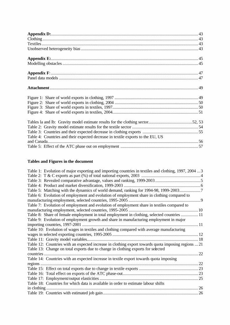
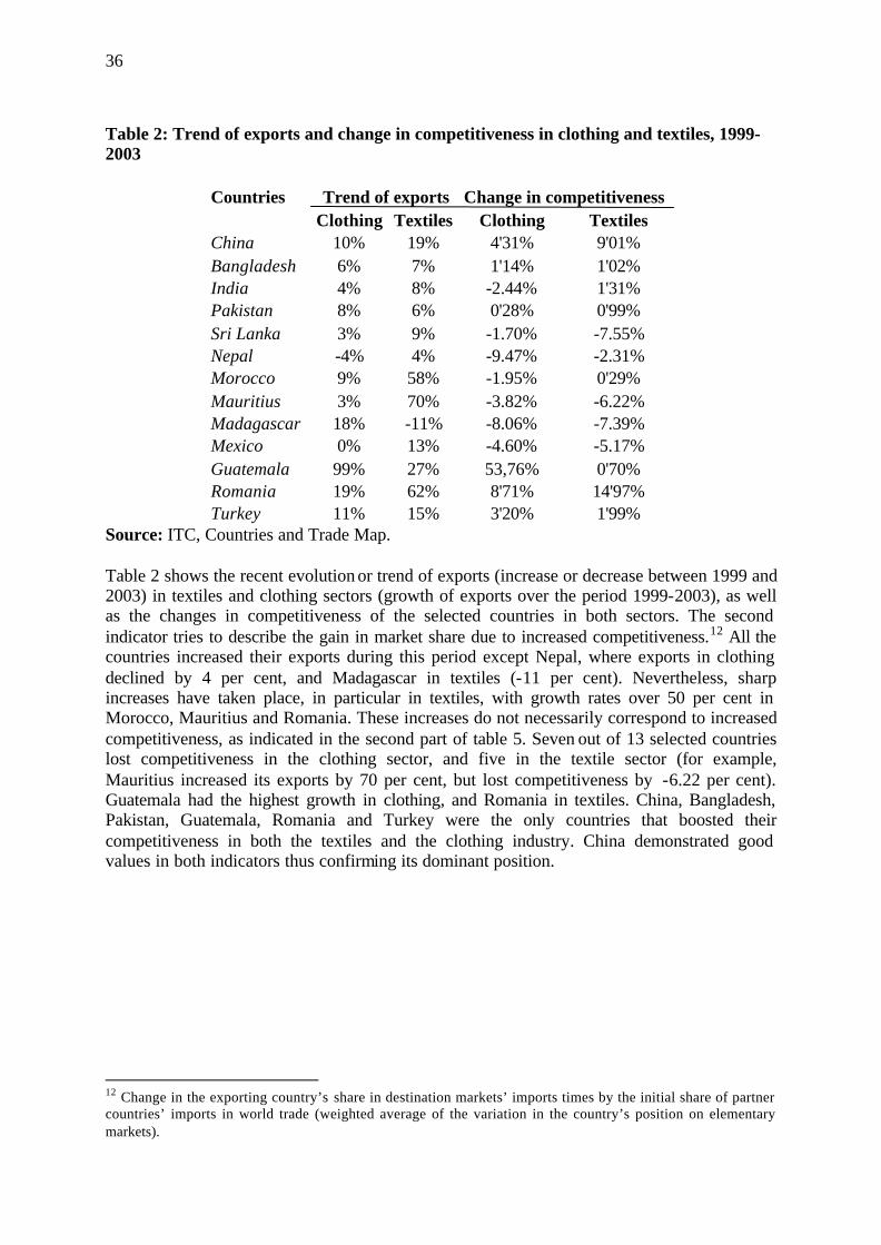
Page Preface Contents Acronyms 1. Introduction ..........................................................................................................................1 2. Recent evolution of trade in major exporting countries...........................................................2 2.1 Evolution of trade flows...........................................................................................................2 2.2 Export performance of selected countries ..................................................................................5 3. The employment situation of selected countries.......................................................................9 4. A gravity model approach forecasting future evolution of trade and employment due to the fadeout of the ATC .......................................................................................................... 13 4.1 The quota system of the ATC................................................................................................. 13 4.2 A gravity model approach to forecast trade shifts..................................................................... 17 4.2.1 The model................................................................................................................... 17 4.2.2 Trade results ............................................................................................................... 20 4.3 Trade shifts and their impact on employment .......................................................................... 24 4.3.1 Calculation of the link between trade and employment................................................... 24 4.3.2 Results........................................................................................................................ 26 5. Conclusion............................................................................................................................. 27 Bibliography .............................................................................................................................. 31 Data Sources .............................................................................................................................. 33 Appendix A ............................................................................................................................... 35 Table 1: World market share and its evolution in textiles and clothing, 1999-2003 .......................... 35 Table 2: Trend of exports and change in competitiveness in clothing and textiles, 1999-2003................................................................................................................................... 36 Appendix B : ............................................................................................................................. 37 Simple model of quota removal redistribution effects ..................................................................... 37 Appendix C: ............................................................................................................................. 39 Quota impact indicator ................................................................................................................. 39 Table 1: Selected sample from US 2003 quota regime ................................................................... 39 Figures 1 and 2: Quota impacts on textiles and clothing over time (1993-2004), USA, Canada and European Union ............................................................................................... 41

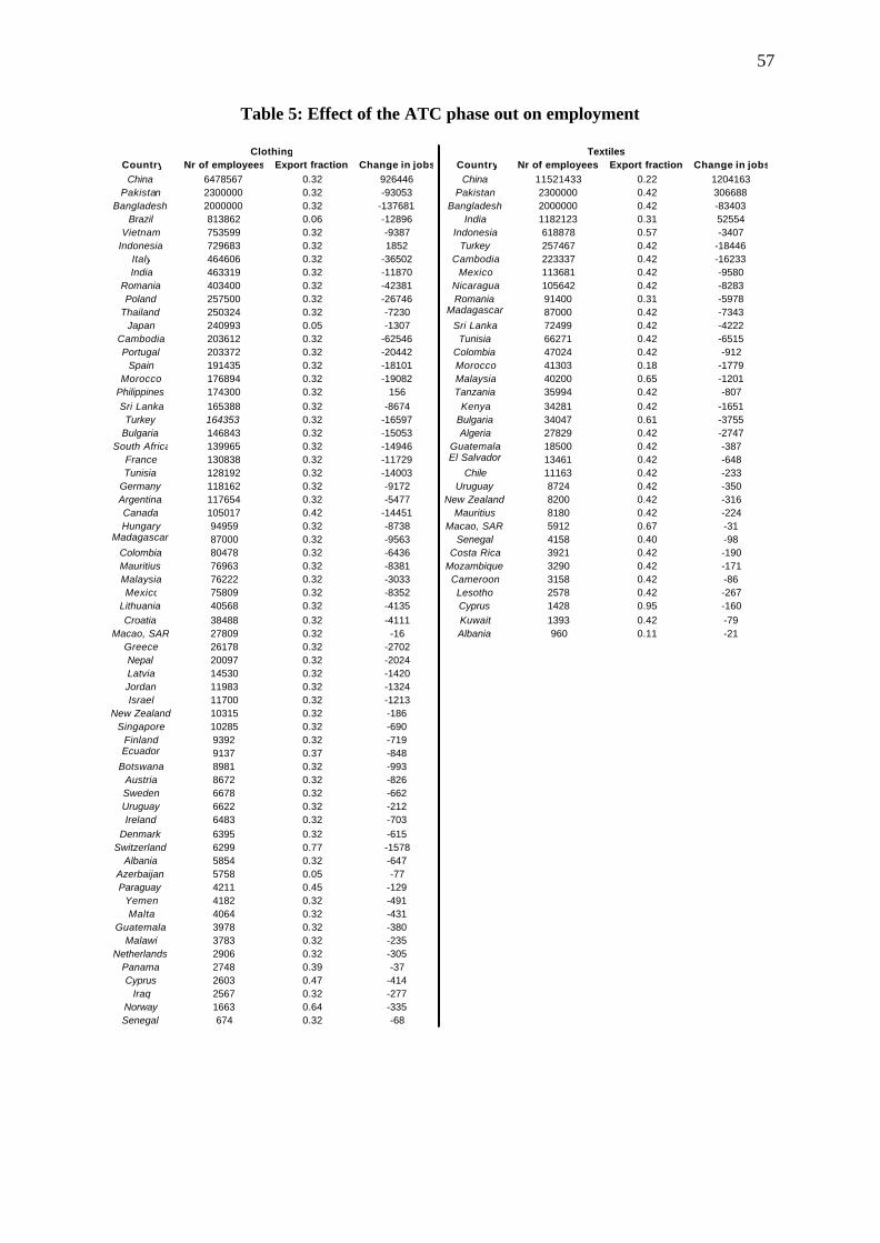
Appendix D:............................................................................................................................... 43 Clothing ...................................................................................................................................... 43 Textiles ....................................................................................................................................... 43 Unobserved heterogeneity bias ..................................................................................................... 43 Appendix E:............................................................................................................................... 45 Modelling obstacles ..................................................................................................................... 45 Appendix F: ............................................................................................................................... 47 Panel data models ........................................................................................................................ 47 Attachment ................................................................................................................................ 49 Figure 1: Share of world exports in clothing, 1997 ........................................................................ 49 Figure 2: Share of world exports in clothing, 2004 ........................................................................ 50 Figure 3: Share of world exports in textiles, 1997.......................................................................... 50 Figure 4: Share of world exports in textiles, 2004.......................................................................... 51 Tables la and lb: Gravity model estimate results for the clothing sector......................................52, 53 Table 2: Gravity model estimate results for the textile sector ......................................................... 54 Table 3: Countries and their expected decrease in clothing exports ................................................ 55 Table 4: Countries and their expected decrease in textile exports to the EU, US and Canada.................................................................................................................................. 56 Table 5: Effect of the ATC phase out on employment ................................................................... 57 Tables and Figures in the document Table 1: Evolution of major exporting and importing countries in textiles and clothing, 1997, 2004 ...3 Table 2: T & C exports as part (%) of total national exports, 2003 ...................................................4 Table 3: Revealed comparative advantage, values and ranking, 1999-2003 .......................................5 Table 4: Product and market diversification, 1999-2003 ..................................................................6 Table 5: Matching with the dynamics of world demand, ranking for 1994-98, 1999-2003..................7 Table 6: Evolution of employment and evolution of employment share in clothing compared to manufacturing employment, selected countries, 1995-2005 ..............................................................9 Table 7: Evolution of employment and evolution of employment share in textiles compared to manufacturing employment, selected countries, 1995-2005 ............................................................10 Table 8: Share of female employment in total employment in clothing, selected countries ............... 11 Table 9: Evolution of employment growth and share in manufacturing employment in major importing countries, 1997-2001 .................................................................................................... 11 Table 10: Evolution of wages in textiles and clothing compared with average manufacturing wages in selected exporting countries, 1995-2005 .......................................................................... 12 Table 11: Gravity model variables................................................................................................ 18 Table 12: Countries with an expected increase in clothing export towards quota imposing regions ... 21 Table 13: Change on total exports due to change in clothing exports for selected countries ..................................................................................................................................... 22 Table 14: Countries with an expected increase in textile export towards quota imposing regions ........................................................................................................................................ 22 Table 15: Effect on total exports due to change in textile exports ................................................... 23 Table 16: Total effect on exports of the ATC phase-out................................................................. 23 Table 17: Employment/output elasticities ..................................................................................... 25 Table 18: Countries for which data is available in order to estimate labour shifts in clothing ................................................................................................................................... 26 Table 19: Countries with estimated job gain .................................................................................. 26

Table 20: Estimated effect of the ATC phase out on employment ................................................... 27 Figure 1: Evolution of world exports in textiles and clothing, 30 major exporting countries, in millions of US$, 1997-2004........................................................................................................2 Figures 2 and 3: Ten most restricted countries in absolute textiles and clothing exports in 2004 ....... 15 Figures 4 and 5: Ten most restricted countries in relative textiles and clothing exports in 2004........................................................................................................................................ 16 Figure 6: Output – employment relationship ................................................................................. 25

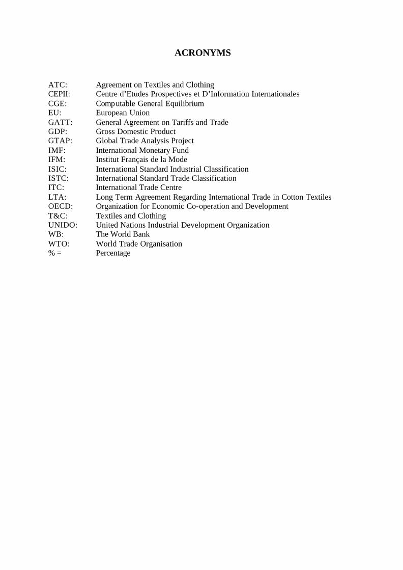
ACRONYMS

ATC: Agreement on Textiles and Clothing CEPII: Centre d’Etudes Prospectives et D’Information Internationales CGE: Computable General Equilibrium EU: European Union GATT: General Agreement on Tariffs and Trade GDP: Gross Domestic Product GTAP: Global Trade Analysis Project IMF: International Monetary Fund IFM: Institut Français de la Mode ISIC: International Standard Industrial Classification ISTC: International Standard Trade Classification ITC: International Trade Centre LTA: Long Term Agreement Regarding International Trade in Cotton Textiles OECD: Organization for Economic Co-operation and Development T&C: Textiles and Clothing UNIDO: United Nations Industrial Development Organization WB: The World Bank WTO: World Trade Organisation % = Percentage

1

1. Introduction

The textiles and clothing industry was, until recently, the only major manufacturing industry that was not subject to the rules of the General Agreement on Tariffs and Trade (GATT). Instead, it was subject to extensive use of quotas by the major importing countries. The quota system started with the Long Term Agreement Regarding International Trade in Cotton Textiles (LTA) under the auspices of the GATT in 1962. In 1974 the LTA was extended to cover other materials than cotton, and became known as the Multi-Fibre Agreement (MFA). At the end of the Uruguay Round of negotiations it was agreed tha t countries wishing to retain quotas would commit themselves to phasing them out gradually over a 10 year period, with the last quotas being lifted 1st of January 2005, as stated in the Agreement on Textiles and Clothing (ATC). The end of the MFA in 2005 will change world trade significantly and, as a result, lead to shifts in world employment. However, the last three decades have seen various changes in the clothing and textile sector, thus forcing many countries to adjust to a constantly altering environment. Now, a number of countries fear that a new wave of cheap textile and clothing products will flood their markets, threatening their domestic industries that are not adequately prepared to face the new challenge. There are also those countries that hope for new export opportunities as a result of a free quota trade environment and a third set of countries that will lose their preferential access to the US or EU markets, thus facing higher competition for their exports to them. Some countries may be able to maintain their industry, successfully adjusting to the new situation, other countries may have to abandon theirs and specialize in other sectors. What is clear is that the textiles and clothing (T&C) world has become a more open market, subject to stronger price and quality competition. Relatively high cost producers, who were able to survive under the ATC regime, may now find it difficult to maintain their position. Intense price competition could force companies to reorganise in order to achieve cost reductions, thereby putting downward pressure on wages and working conditions (see appendix A for a simple mathematical model). The group benefiting from this trend are the T&C consumers. Producers may gain in the short term, due to increased market share, but their profits could decrease due to lower prices. Some workers may be disadvantaged by increased competition in wage and labour conditions. Others may find a better paid job in T&C. The following study will describe the evolution of trade and employment in the T&C during recent years until June 2005. The main focus of this chapter is on exporting developing countries. The first part of this study describes the evolution of performance in trade in the textiles and clothing industry of major exporting countries just before the completion of the phasing out period in 2005. It shows the already leading, and increasing position, of China and China, including Hong Kong, SAR, and Macao, SAR, in particular in clothing, Pakistan’s dominant position in textiles and the good trade performance in general of South and South East Asia. It is striking that some countries with a relatively poor trade performance, mainly from Central America and Africa are specialized in the T&C industry, benefiting from special trade agreements. A second chapter describes the employment situation during the last years of major exporting, but also importing countries. Emerging countries in South and South East Asia, in particular China, but also some African and Central American countries, increased employment significantly in this industry, while employment in OECD countries declined. The third chapter attempts to forecast trade and employment changes due to the change in

2

trade regime from the 1st of January 2005 in the world of T&C, by using a gravity model approach. From this we see that both China and Pakistan might benefit considerably from the MFA phase-out, that there is a group of countries that will probably benefit, but not excessively and yet another large group of T&C exporting countries that will lose part of their share in exports towards the quota imposing countries.

2. Recent evolution of trade in major exporting countries

2.1. Evolution of trade flows The quota regime of the MFA has represented a major obstacle to world trade in textiles and clothing and distorted world trade towards countries with protected industries and others with preferential access to the major market of destination, mainly the US and the EU market, but also Norway and Canada.

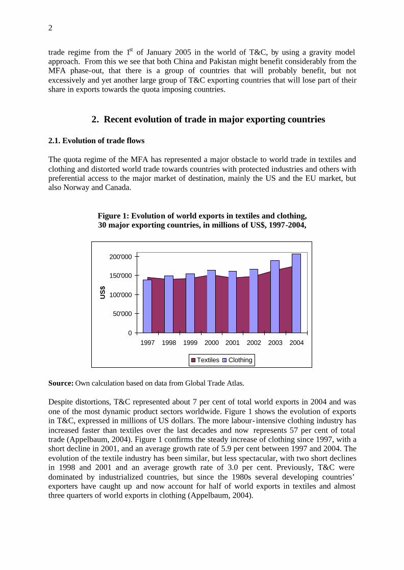
Figure 1: Evolution of world exports in textiles and clothing, 30 major exporting countries, in millions of US$, 1997-2004,

0

50'000

100'000

150'000

200'000

1997 1998 1999 2000 2001 2002 2003 2004

US

$

Textiles Clothing

Source: Own calculation based on data from Global Trade Atlas. Despite distortions, T&C represented about 7 per cent of total world exports in 2004 and was one of the most dynamic product sectors worldwide. Figure 1 shows the evolution of exports in T&C, expressed in millions of US dollars. The more labour- intensive clothing industry has increased faster than textiles over the last decades and now represents 57 per cent of total trade (Appelbaum, 2004). Figure 1 confirms the steady increase of clothing since 1997, with a short decline in 2001, and an average growth rate of 5.9 per cent between 1997 and 2004. The evolution of the textile industry has been similar, but less spectacular, with two short declines in 1998 and 2001 and an average growth rate of 3.0 per cent. Previously, T&C were dominated by industrialized countries, but since the 1980s several developing countries’ exporters have caught up and now account for half of world exports in textiles and almost three quarters of world exports in clothing (Appelbaum, 2004).

3

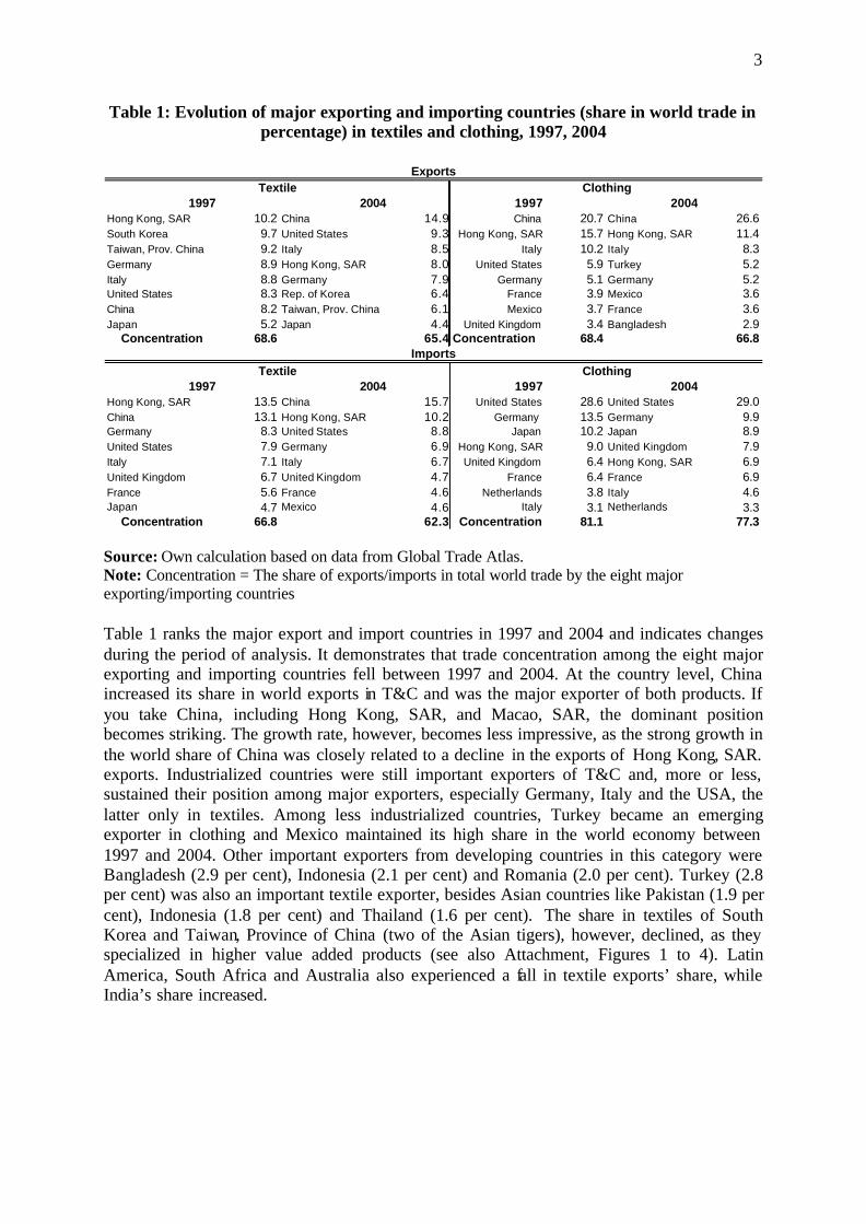
Table 1: Evolution of major exporting and importing countries (share in world trade in percentage) in textiles and clothing, 1997, 2004

1997 2004 1997 2004Hong Kong, SAR 10.2 China 14.9 China 20.7 China 26.6South Korea 9.7 United States 9.3 Hong Kong, SAR 15.7 Hong Kong, SAR 11.4Taiwan, Prov. China 9.2 Italy 8.5 Italy 10.2 Italy 8.3Germany 8.9 Hong Kong, SAR 8.0 United States 5.9 Turkey 5.2Italy 8.8 Germany 7.9 Germany 5.1 Germany 5.2United States 8.3 Rep. of Korea 6.4 France 3.9 Mexico 3.6China 8.2 Taiwan, Prov. China 6.1 Mexico 3.7 France 3.6Japan 5.2 Japan 4.4 United Kingdom 3.4 Bangladesh 2.9

Concentration 68.6 65.4 Concentration 68.4 66.8

1997 2004 1997 2004Hong Kong, SAR 13.5 China 15.7 United States 28.6 United States 29.0China 13.1 Hong Kong, SAR 10.2 Germany 13.5 Germany 9.9Germany 8.3 United States 8.8 Japan 10.2 Japan 8.9United States 7.9 Germany 6.9 Hong Kong, SAR 9.0 United Kingdom 7.9Italy 7.1 Italy 6.7 United Kingdom 6.4 Hong Kong, SAR 6.9United Kingdom 6.7 United Kingdom 4.7 France 6.4 France 6.9France 5.6 France 4.6 Netherlands 3.8 Italy 4.6Japan 4.7 Mexico 4.6 Italy 3.1 Netherlands 3.3

Concentration 66.8 62.3 Concentration 81.1 77.3

Textile Clothing

ExportsTextile Clothing

Imports

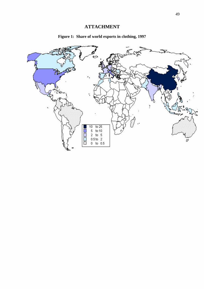
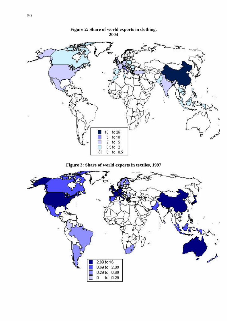
Source: Own calculation based on data from Global Trade Atlas. Note: Concentration = The share of exports/imports in total world trade by the eight major exporting/importing countries Table 1 ranks the major export and import countries in 1997 and 2004 and indicates changes during the period of analysis. It demonstrates that trade concentration among the eight major exporting and importing countries fell between 1997 and 2004. At the country level, China increased its share in world exports in T&C and was the major exporter of both products. If you take China, including Hong Kong, SAR, and Macao, SAR, the dominant position becomes striking. The growth rate, however, becomes less impressive, as the strong growth in the world share of China was closely related to a decline in the exports of Hong Kong, SAR. exports. Industrialized countries were still important exporters of T&C and, more or less, sustained their position among major exporters, especially Germany, Italy and the USA, the latter only in textiles. Among less industrialized countries, Turkey became an emerging exporter in clothing and Mexico maintained its high share in the world economy between 1997 and 2004. Other important exporters from developing countries in this category were Bangladesh (2.9 per cent), Indonesia (2.1 per cent) and Romania (2.0 per cent). Turkey (2.8 per cent) was also an important textile exporter, besides Asian countries like Pakistan (1.9 per cent), Indonesia (1.8 per cent) and Thailand (1.6 per cent). The share in textiles of South Korea and Taiwan, Province of China (two of the Asian tigers), however, declined, as they specialized in higher value added products (see also Attachment, Figures 1 to 4). Latin America, South Africa and Australia also experienced a fall in textile exports’ share, while India’s share increased.

4

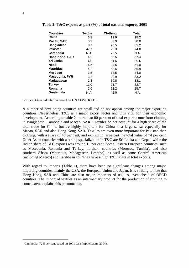
Table 2: T&C exports as part (%) of total national exports, 2003

Countries Textile Clothing TotalChina 6.3 11.9 18.2Macau, SAR 0.9 89.9 90.8Bangladesh 8.7 76.5 85.2Pakistan 47.7 26.3 74.0Cambodia N.A. 72.5 N.A.Hong Kong, SAR 4.9 52.5 57.4Sri Lanka 4.0 51.6 55.6Nepal 16.5 34.5 51.0Mauritius 4.2 52.6 56.9Morocco 1.5 32.5 34.0Macedonia, FYR 3.2 30.0 33.2Madagascar 2.3 30.8 33.1Turkey 11.0 21.7 32.7Romania 2.6 23.2 25.7Guatemala N.A. 42.0 N.A.

Source: Own calculation based on UN COMTRADE. A number of developing countries are small and do not appear among the major exporting countries. Nevertheless, T&C is a major export sector and thus vital for their economic development. According to table 2, more than 80 per cent of total exports come from clothing in Bangladesh, Cambodia and Macao, SAR.1 Textiles do not account for a high share of the total trade for China, but are highly important for China in a large sense, especially for Macao, SAR and also Hong Kong, SAR. Textiles are even more important for Pakistan than clothing, with a share of 48 per cent, and explain in large part the total value of 74 per cent. Other Asian countries with a strong specialization in T&C are Sri Lanka and Nepal, while the Indian share of T&C exports was around 15 per cent. Some Eastern European countries, such as Macedonia, Romania and Turkey, northern countries (Morocco, Tunisia), and also southern Africa (Mauritius, Madagascar, Lesotho), as well as some Central American (including Mexico) and Caribbean countries have a high T&C share in total exports. With regard to imports (Table 1), there have been no significant changes among major importing countries, mainly the USA, the European Union and Japan. It is striking to note that Hong Kong, SAR and China are also major importers of textiles, even ahead of OECD countries. The import of textiles as an intermediary product for the production of clothing to some extent explains this phenomenon.

1 Cambodia: 72.5 per cent based on 2001 data (Appelbaum, 2004).

5

2.2. Export performance of selected countries An analysis of the trade structure, with the help of various export performance indicators, is essential to understanding the evolution of recent trade flows.

Table 3: Revealed comparative advantage, values and ranking, 1999-2003

Countries

Value Ranking Value RankingChina 3'46 33 2'39 10Bangladesh 23'58 4 2'28 12India 3'09 38 4'27 7Pakistan 7'99 22 18'93 1Sri Lanka 16'17 7 1'24 33Nepal 9'20 18 10'27 2Morocco 0.58 71 9.63 15Mauritius 15'33 8 1'59 26Madagascar 9'01 19 0'51 76Mexico 1'29 61 0'49 81Guatemala 1'14 63 0'77 53Romania 6'75 25 0'98 39Turkey 4'40 6 6'22 26

TextilesClothing

Source: ITC, Countries and Trade Map.

One way to compare the export performance of major exporting countries is to analyze their revealed comparative advantage. This indicator describes the sectoral trade specialization according to the Balassa formula. It shows in which export sector a country is most specialized compared to other tradable goods and countries. It shows the export performance of a country compared with other countries. The deficit of this indicator is that it refers to actual trade flows and, to a certain extent, does not show the real trade potential of each country. China, for example, is only ranked 33 for clothing and 10 for textiles during the 1999-2003 period (Table 3), but it is also the country most affected by quota restrictions. Future data will certainly show better values for China. An analysis of this indicator reveals a strong comparative advantage for Pakistan in textiles, ranked number one, and Nepal, ranked second, but also for India and Morocco. Bangladesh is well positioned in both products, in particular in clothing, while Sri Lanka and Turkey have a strong comparative advantage only in clothing. Mauritius is strongly specialized in clothing and is also relatively well positioned as a textile exporter. In Latin America, however, important exporting countries, such as Mexico and Guatemala, have a relatively low comparative advantage in textiles and clothing. Romania is better placed and has a relatively good comparative advantage, particularly in clothing.

6

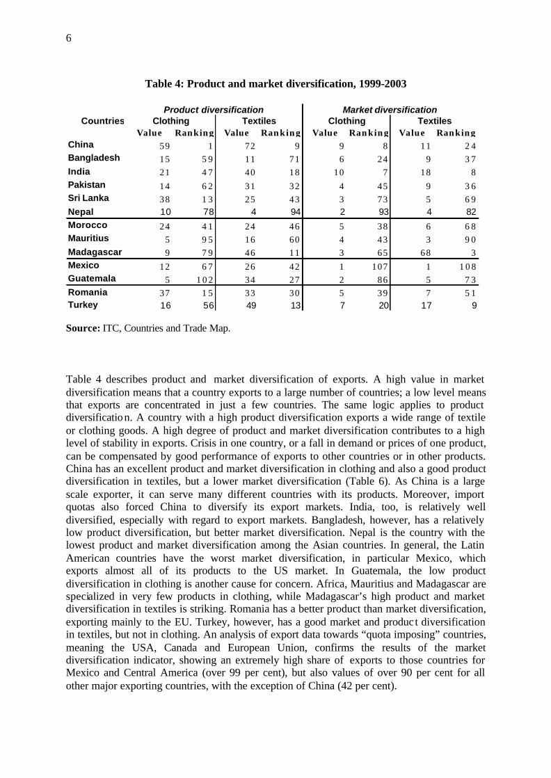
Table 4: Product and market diversification, 1999-2003

CountriesValue Ranking Value Ranking Value Ranking Value Ranking

China 59 1 72 9 9 8 11 24Bangladesh 15 59 11 71 6 24 9 37India 21 47 40 18 10 7 18 8Pakistan 14 62 31 32 4 45 9 36Sri Lanka 38 13 25 43 3 73 5 69Nepal 10 78 4 94 2 93 4 82Morocco 24 41 24 46 5 38 6 68Mauritius 5 95 16 60 4 43 3 90Madagascar 9 79 46 11 3 65 68 3Mexico 12 67 26 42 1 107 1 108Guatemala 5 102 34 27 2 86 5 73Romania 37 15 33 30 5 39 7 51Turkey 16 56 49 13 7 20 17 9

Product diversification Market diversificationClothing Textiles Clothing Textiles

Source: ITC, Countries and Trade Map. Table 4 describes product and market diversification of exports. A high value in market diversification means that a country exports to a large number of countries; a low level means that exports are concentrated in just a few countries. The same logic applies to product diversification. A country with a high product diversification exports a wide range of textile or clothing goods. A high degree of product and market diversification contributes to a high level of stability in exports. Crisis in one country, or a fall in demand or prices of one product, can be compensated by good performance of exports to other countries or in other products. China has an excellent product and market diversification in clothing and also a good product diversification in textiles, but a lower market diversification (Table 6). As China is a large scale exporter, it can serve many different countries with its products. Moreover, import quotas also forced China to diversify its export markets. India, too, is relatively well diversified, especially with regard to export markets. Bangladesh, however, has a relatively low product diversification, but better market diversification. Nepal is the country with the lowest product and market diversification among the Asian countries. In general, the Latin American countries have the worst market diversification, in particular Mexico, which exports almost all of its products to the US market. In Guatemala, the low product diversification in clothing is another cause for concern. Africa, Mauritius and Madagascar are specialized in very few products in clothing, while Madagascar’s high product and market diversification in textiles is striking. Romania has a better product than market diversification, exporting mainly to the EU. Turkey, however, has a good market and produc t diversification in textiles, but not in clothing. An analysis of export data towards “quota imposing” countries, meaning the USA, Canada and European Union, confirms the results of the market diversification indicator, showing an extremely high share of exports to those countries for Mexico and Central America (over 99 per cent), but also values of over 90 per cent for all other major exporting countries, with the exception of China (42 per cent).

7

Table 5: Matching with the dynamics of world demand, ranking for 1994-98, 1999-2003

Countries 1994-98 1999-2003 1994-98 1999-2003

China 80 26 84 10Bangladesh 77 40 22 12

India 116 115 90 56Pakistan 101 16 59 43

Sri Lanka 22 70 87 24Nepal 109 28 89 38

Morocco 57 66 26 75Mauritius 21 43 60 46

Madagascar 78 37 110 6Mexico 29 59 3 28

Guatemala 48 63 71 59Romania 56 91 73 40

Turkey 54 49 12 23

Clothing Textiles

Ranking

Source: ITC, Countries and Trade Map. A specialization in specific products is even more fruitful, if it occurs in products where the world demand is strong and increasing. The ranking in Table 5 shows the evolution of each country with regard to its specialization in dynamic products where the demand in importing countries shows an increasing trend. Once again, China is well placed and strongly improved its specialization in dynamic goods, from rank 80 in 1994-98 to rank 26 in clothing in 1999-2003, in textiles from rank 84 in 1994-98 to rank 10 in 1999-2003. Bangladesh and Nepal in particular, but also Pakistan, have intensified their specialization in dynamic goods during the period of analysis. India, however, is poorly placed, particularly in clothing, but also in textiles, even though it has improved its ranking in the latter. Mexico, Guatemala, Mauritius and Sri Lanka were the major losers in clothing, while Madagascar, South Asia and China were the major winners. In textiles, the situation was a bit different. Sri Lanka now appears among the winners, together with the other Asian countries mentioned, although Madagascar, Mauritius, Guatemala and Romania produced more dynamic goods. Mexico, once again, produced less dynamic textile goods as did Morocco and Turkey, but the latter was still well positioned.2 Nevertheless, the competitiveness of the T&C industry at the international level depends on various other factors, not directly trade related: Ø Labour cost: The USA and Germany have the highest labour costs according to a

recent calculation by Appelbaum (2004), but they are still important exporters in the T&C industry. High productivity and specialization in specific high quality segments explains this positive result. Nevertheless, major low labour cost countries are among

2 In the appendix A, table 1 and 2 you will find additional information on the trade performance, in particular on: world market share and its evolution, trends of exports and change in competit iveness.

8

the main exporting countries. Pakistan benefits from the lowest labour costs, followed by Indonesia, Sir Lanka, India and China.

Ø Quality and availability of appropriately skilled workforce. Ø Other production costs: energy, water, production inputs (e.g. cotton, polyester),

chemicals and construction. Ø Production processes: full-package production systems versus captive networks,

where producers are just limited to assembly or cut fabrics Ø Transport (shipping costs and time) and distribution. Ø FDI, strategic alliances. Ø Macroeconomic environment: domestic interest rates, income and corporate taxes,

exchange rate and public support to the industry, preferential access to markets, country risk (property rights, political stability).

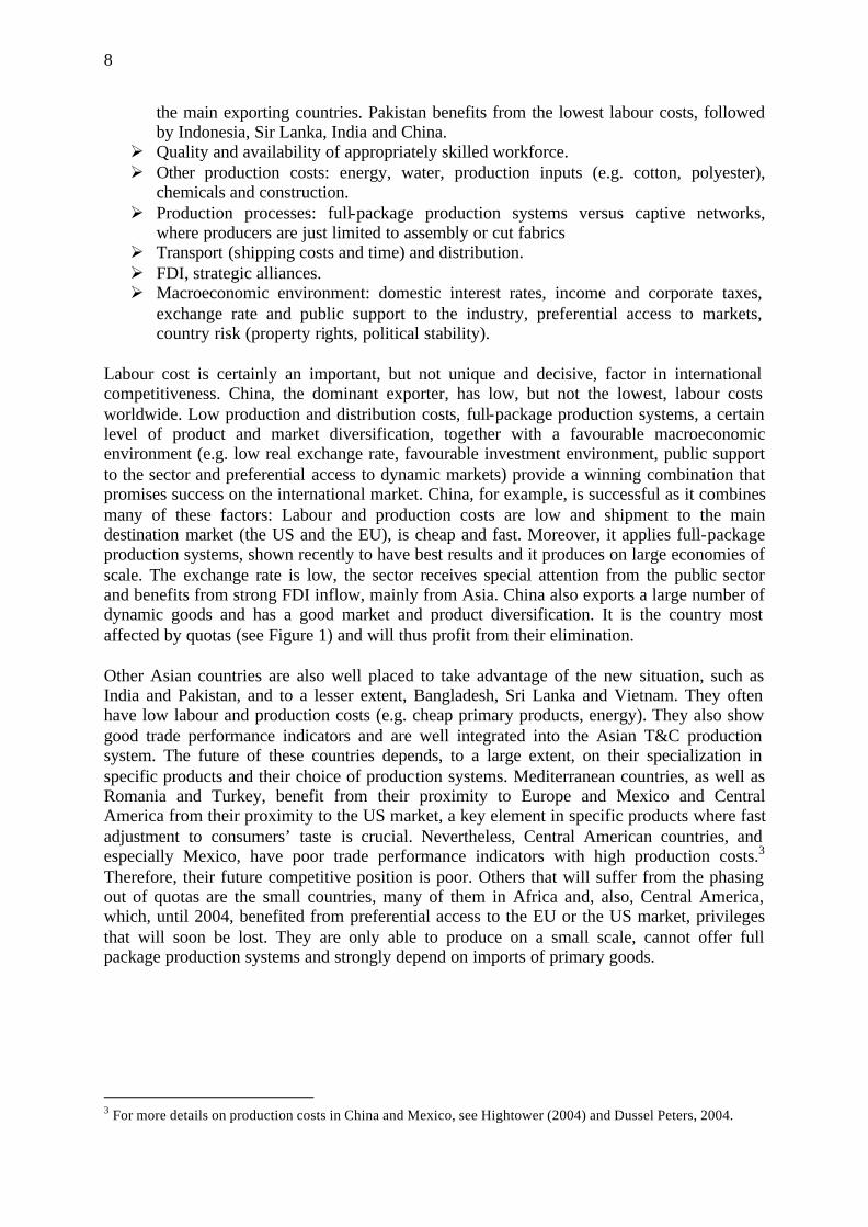
Labour cost is certainly an important, but not unique and decisive, factor in international competitiveness. China, the dominant exporter, has low, but not the lowest, labour costs worldwide. Low production and distribution costs, full-package production systems, a certain level of product and market diversification, together with a favourable macroeconomic environment (e.g. low real exchange rate, favourable investment environment, public support to the sector and preferential access to dynamic markets) provide a winning combination that promises success on the international market. China, for example, is successful as it combines many of these factors: Labour and production costs are low and shipment to the main destination market (the US and the EU), is cheap and fast. Moreover, it applies full-package production systems, shown recently to have best results and it produces on large economies of scale. The exchange rate is low, the sector receives special attention from the public sector and benefits from strong FDI inflow, mainly from Asia. China also exports a large number of dynamic goods and has a good market and product diversification. It is the country most affected by quotas (see Figure 1) and will thus profit from their elimination. Other Asian countries are also well placed to take advantage of the new situation, such as India and Pakistan, and to a lesser extent, Bangladesh, Sri Lanka and Vietnam. They often have low labour and production costs (e.g. cheap primary products, energy). They also show good trade performance indicators and are well integrated into the Asian T&C production system. The future of these countries depends, to a large extent, on their specialization in specific products and their choice of production systems. Mediterranean countries, as well as Romania and Turkey, benefit from their proximity to Europe and Mexico and Central America from their proximity to the US market, a key element in specific products where fast adjustment to consumers’ taste is crucial. Nevertheless, Central American countries, and especially Mexico, have poor trade performance indicators with high production costs.3 Therefore, their future competitive position is poor. Others that will suffer from the phasing out of quotas are the small countries, many of them in Africa and, also, Central America, which, until 2004, benefited from preferential access to the EU or the US market, privileges that will soon be lost. They are only able to produce on a small scale, cannot offer full package production systems and strongly depend on imports of primary goods.

3 For more details on production costs in China and Mexico, see Hightower (2004) and Dussel Peters, 2004.

9

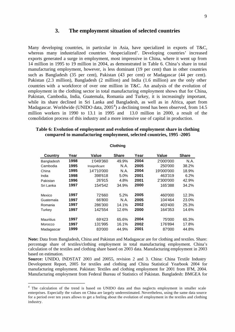
3. The employment situation of selected countries Many developing countries, in particular in Asia, have specialized in exports of T&C, whereas many industrialized countries ‘despecialized’. Developing countries’ increased exports generated a surge in employment, most impressive in China, where it went up from 14 million in 1995 to 19 million in 2004, as demonstrated in Table 6. China’s share in total manufacturing employment, however, is less dominant (19 per cent) than in other countries such as Bangladesh (35 per cent), Pakistan (43 per cent) or Madagascar (44 per cent). Pakistan (2.3 million), Bangladesh (2 million) and India (1.6 million) are the only other countries with a workforce of over one million in T&C. An analysis of the evolution of employment in the clothing sector in total manufacturing employment shows that for China, Pakistan, Cambodia, India, Guatemala, Romania and Turkey, it is increasingly important, while its share declined in Sri Lanka and Bangladesh, as well as in Africa, apart from Madagascar. Worldwide (UNIDO data, 20054) a declining trend has been observed, from 14.5 million workers in 1990 to 13.1 in 1995 and 13.0 million in 2000, a result of the consolidation process of this industry and a more intensive use of capital in production.

Table 6: Evolution of employment and evolution of employment share in clothing compared to manufacturing employment, selected countries, 1995 -2005

Country Year Value Share Year Value ShareBangladesh 1998 1'049'360 49.9% 2004 2'000'000 N.A.Cambodia 1995 Insignificant N.A. 2005 250'000 38.2%China 1995 14'710'000 N.A. 2004 19'000'000 18.9%India 1998 398'618 5.0% 2001 463'319 6.2%Pakistan 1996 26'915 4.8% 2001 2'300'000 42.9%Sri Lanka 1997 154'542 34.9% 2000 165'388 34.2%

Mexico 1997 72'660 5.2% 2005 460'000 12.3%Guatemala 1997 66'800 N.A. 2005 104'464 23.0%Romania 1997 286'300 14.1% 2002 403'400 25.3%Turkey 1997 142'554 12.6% 2000 164'353 14.6%

Mauritius 1997 69'423 65.6% 2004 75'000 65.3%Morocco 1997 131'995 16.1% 2002 176'894 17.8%Madagascar 1999 83'000 44.9% 2001 87'000 44.8%

Clothing

Note: Data from Bangladesh, China and Pakistan and Madagascar are for clothing and textiles. Share: percentage share of textiles/clothing employment in total manufacturing employment. China’s calculation of the textiles and clothing share based on 2003 data. Manufacturing employment in 2003 based on estimation. Source: UNIDO, INDSTAT 2003 and 20055, revision 2 and 3. China: China Textile Industry Development Report, 2005 for textiles and clothing and China Statistical Yearbook 2004 for manufacturing employment. Pakistan: Textiles and clothing employment for 2001 from IFM, 2004. Manufacturing employment from Federal Bureau of Statistics of Pakistan. Bangladesh: BMGEA for

4 The calculation of the trend is based on UNIDO data and thus neglects employment in smaller scale enterprises. Especially the values on China are largely underestimated. Nevertheless, using the same data source for a period over ten years allows to get a feeling about the evolution of employment in the textiles and clothing industry.

10

2004 data. Guatemala: Asociación Gremial de exportadores de productos no tradicionales. Madagascar: Labour and Social Law Ministry. Mexico, 2005: National Chamber of Textile Industry (including share). Cambodia, 2005: Industry of Commerce (share from 2000 based on UNIDO data). Mauritius, 2004: AfrolNews, 26 September 2005.

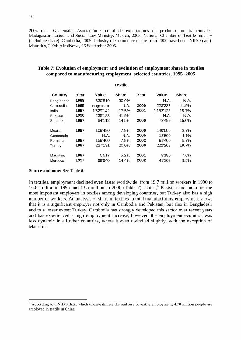
Table 7: Evolution of employment and evolution of employment share in textiles compared to manufacturing employment, selected countries, 1995 -2005

Country Year Value Share Year Value ShareBangladesh 1998 630'810 30.0% N.A. N.A.Cambodia 1995 Insignificant N.A. 2000 223'337 41.9%India 1997 1'529'142 17.5% 2001 1'182'123 15.7%Pakistan 1996 235'183 41.9% N.A. N.A.Sri Lanka 1997 64'112 14.5% 2000 72'499 15.0%

Mexico 1997 109'490 7.9% 2000 140'000 3.7%Guatemala N.A. N.A. 2005 18'500 4.1%Romania 1997 159'400 7.8% 2002 91'400 5.7%Turkey 1997 227'131 20.0% 2000 222'268 19.7%

Mauritius 1997 5'517 5.2% 2001 8'180 7.0%Morocco 1997 68'640 14.4% 2002 41'303 9.5%

Textile

Source and note: See Table 6. In textiles, employment declined even faster worldwide, from 19.7 million workers in 1990 to 16.8 million in 1995 and 13.5 million in 2000 (Table 7). China,5 Pakistan and India are the most important employers in textiles among developing countries, but Turkey also has a high number of workers. An analysis of share in textiles in total manufacturing employment shows that it is a significant employer not only in Cambodia and Pakistan, but also in Bangladesh and to a lesser extent Turkey. Cambodia has strongly developed this sector over recent years and has experienced a high employment increase, however, the employment evolution was less dynamic in all other countries, where it even dwindled slightly, with the exception of Mauritius.

5 According to UNIDO data, which under-estimate the real size of textile employment, 4.78 million people are employed in textile in China.

11

Table 8: Share of female employment in total employment in clothing, selected countries

Country Year ShareBangladesh 2004 80.0Cambodia 2000 89.4India 2003 42.6Sri Lanka 2000 82.4Nepal 2002 15.3Guatemala 2004 50.0Mauritius 1997 73.0Morocco 1997 72.4Romania 2000 54.0Turkey 2000 48.0

Source: UNIDO, Indstat 2005, BGMEA data for Bangladesh. INE for Guatemala (textile and clothing). A phenomenon of the T&C sectors, in particular clothing, is the high percentage share of female workers who are often young and unskilled (Appelbaum, 2004 and Kivik Nordas, 2005). Worldwide, the share increased from 59 per cent in 1990 to 68 per cent in 2000 according to UNIDO data. Table 8 shows that, especially in Asia, the share of female employment is very high with more than 89 per cent in Cambodia, 80 per cent in Bangladesh and 82 per cent in Sri Lanka,6 In Africa too, with 73 per cent in Mauritius and 72 per cent in Morocco (table 6). India and Turkey, however, are below 50 per cent and Guatemala 50 per cent. The female share in textiles is, in general, lower, but increasing from 44 per cent in 1990 to 50 per cent worldwide. Cambodia with 75.9 per cent and Sri Lanka 61.2 per cent are exceptional cases with a high female share. In Nepal, however, neither the clothing (15.3 per cent) nor the textile industry (30.8 per cent in 2002) are dominated by female workers

Table 9: Evolution of employment growth and share in manufacturing employment

in major importing countries, 1997-2001

OECD countries Growth 97-01 Share 1997 Share 2000 Growth 97-01 Share 1997 Share 2001

France -16.1% 3.6% 3.0% -9.9% 3.0% 2.6%Germany -5.7% 1.8% 1.4% 2.8% 2.1% 1.8%Italy 0.6% 11.6% 10.3% -5.4% 6.9% 6.5%Japan -13.8% 3.9% 2.8% -27.8% 4.3% 3.6%United Kingdom -1.2% 4.4% 3.6% -14.5% 4.2% 3.6%United States -35.9% 3.4% 2.4% -20.8% 3.6% 3.0%Canada 10.7% 4.6% 5.1% 4.9% 3.4% 3.2%

Clothing Textile

Note: 2001 data: Canada, Japan, 2000 data: France, Germany, Italy, United Kingdom. Source: UNIDO, Indstat 2005, Revision 3. OECD Labour Market Statistics.

6 In Bangladesh and Sri Lanka, for example, female employment in total manufacturing employment is much lower with 9 and 22 per cent respectively (UNDP, Human Development Indicators 2004).

12

The T&C industry of OECD countries, which are the main importing countries, is expected to suffer significantly from increased competition from developing countries. An analysis of Table 9 shows that major OECD countries already saw a decline in the importance of employment in their T&C industry between 1997 and 2001. This is not just the result of increased productivity, but is also due to a general decline of production in and a deliberate pulling out of this industry. The fall is even more pronounced in textiles, where all selected countries, with the exception of Canada and Germany who both experienced a slow rise, had negative growth rates during the analysis period. Japan and the USA are the most affected by this evolution. The situation was less dramatic in clothing, where in all countries, apart from Canada, the clothing industry lost its importance as an employer. The USA, Japan and France experienced a steep fall in employment in the clothing industry. Italy remained the only OECD country where employment in textiles and clothing was still significantly high within manufacturing employment.

Table 10: Evolution of wages in textiles and clothing compared with average manufacturing wages in selected exporting countries, 1995-2005

Year Wc/Wtot Year Wc/Wtot Year Wt/Wtot Year Wt/WtotBangladesh 1998 76.7% N.A. 1998 90.2% N.A.Cambodia 1995 80.7% 2000 99.8% 1995 89.1% 2000 123.1%China 1997 N.A 2203 38.7% 1997 N.A. 2003 43.3%India 1998 16.2% 58.7% 1997 80.3% 76.1%Pakistan 1996 90.3% 2001 57.2% 1996 69.1% 2001 56.2%Sri Lanka 1997 96.0% 2000 95.1% 1997 86.2% 2000 82.8%

Mexico 1997 51.5% 2000 50.6% 1997 63.9% 2000 64.3%Guatemala 1997 74.8% 1997 67.6% N.A.Mauritius 1997 80.1% 2000 84.1% 1997 101.3% 2000 71.7%Morocco 1997 62.4% 2002 53.4% 1997 77.4% 2002 73.5%Romania 1997 74.6% 2002 54.0% 1997 74.5% 2002 61.3%Turkey 1997 61.8% 2000 50.4% 1997 73.3% 2000 66.0%

Clothing Textile

Note: Wt/Wtot: average wage in textile (Wt) compared with average wage in manufacturing (Wtot) as a share value. Wc = average wage in clothing. Source : UNIDO, Indstat 2005, Rev. 2 and 3. Pakistan, ILO Laborsta. Table 10 displays some interesting results in terms of the quality of employment showing the difference between the wages in clothing or textiles and the average manufacturing wage. A value of 90 per cent means, for example, that the wages in this sector correspond to 90 per cent of the average wage in the manufacturing sector. As expected, workers in the T&C industry earn a lower wage than that of a manufacturing worker, as this industry produces low value goods and employs a mainly unskilled workforce. The situation, however, worsened, particularly in textiles, between the end of the 1990s and the beginning of the new millennium, as highlighted in Table 10. This can be attributed, in part, to fiercer global competition and thus downward pressure on wages. Only in a few countries did the gap narrow between wages in the T&C industry and manufacturing. For example, in India and Mauritius in clothing and, in particular, in Cambodia where wages increased in clothing and in textiles (123 per cent) were even higher than average wages in manufacturing.

13

4. A gravity model approach forecasting future evolution of trade and employment due to the fadeout of the ATC

4.1. The quota system of the ATC Three regions, Canada, EU and USA, chose to maintain quotas under the ATC unt il January 2005. These countries have allocated quotas to trading partners unilaterally. At the same time they have awarded trading partners quota-free and sometimes tariff- free access to their markets through regional trade agreements or various preference schemes for developed and least developed countries. The resulting trade regime was highly distorted and unpredictable, particularly from the point of view of exporters who faced binding quotas. As a result significant clothing exporting industries were established in preference-receiving countries, based on comfortable preference margins. With the phasing out of quotas preferences are eroded and it is feared that jobs could be lost on a massive scale in these countries post ATC. Although Norway removed all its quotas in 2003,7 the other three quota restricting regions have followed to the letter ATC in such a way that binding quotas still covered around 80 per cent of the imported products until the very last day of the adjustment period, resulting in back-loading and a drastic change of trade regime from 1st of January 2005. In order to measure the global impact of the fadeout, from 1990 till 2002, 16 global quantitative studies (OECD, 2004) were performed. All these studies were based on Computable General Equilibrium Models and resulted in forecasts of trade shifts and welfare gains. Only one of these studies concerns labour, Lankes (IMF, 2002), using a Global Trade Analysis Project (GTAP), suggests that the quotas led to 19 million fewer jobs in developing countries. The most comprehensive study providing labour shift estimates is IFM (2004). The forecasts are a result from the dynamic general equilibrium model named MIRAGE (CEPII, 2002). The result of this study is that all regions, except for China and India which gain jobs in both the textile and clothing sector, lose jobs. There are, however, a number of reasons why further research is recommended. Most importantly, the MIRAGE and other CGE models assume full employment (OECD, 2004) and do not take proximity to markets into account (Nordas, 2004). The full employment assumption is unrealistic, since many clothing and textiles exporting countries are in the majority developing countries with high unemployment and underemployment rates. Also, ignoring the influence of proximity to markets leads to different results, due to the influence on trade of transportation costs and delivery time. Gravity model analysis suggests that trade decreases at a rate of between 10 and 15 percent for a 10 per cent distance increase. Furthermore, the analyses are not at the country level, but in 7 regions 8 which excludes the possibility of specific countries with different outcomes in countries surrounding the regions. In this paper a quantitative method is used that overcomes these drawbacks and is well known in trade analyses as the gravity model. It is based on the gravity principle which states that mass attracts. It incorporates proximity, assumes nothing about the employment percentage

7 For further discussion on the effects of the MFA phase out in Norway, see Nordas (2004). 8 EU 15, New EU members, NAFTA, China, India, Turkey, North Africa.

14

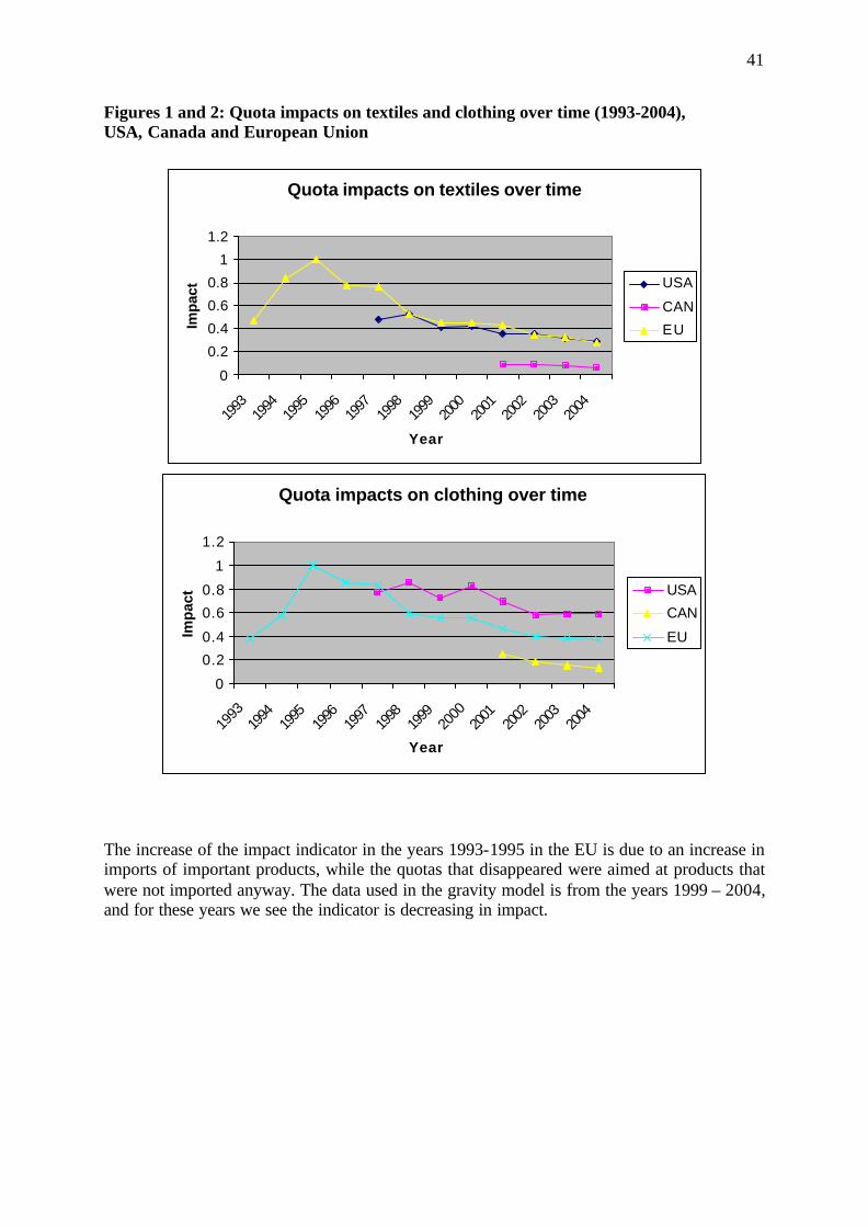
and goes to the country level. Nobel Laureate Jan Tinbergen (1962) was the first to publish an econometric study using the gravity equation for international trade flows, and since then it has developed as the empirical workhorse of international trade (Bayoumi and Eichengreen, 1997). It incorporates proximity as an explanatory variable, and assumes nothing about the degree of employment. The empirical success of the gravity model for explaining and predicting cross sectional international trade pattern levels is well documented and has a rich history; see Baldwin (1994); Oguledo and MacPhee (1994); Deardorff (1995) and Frankel (1997), for useful surveys. Using a gravity model has its strengths, but also its weaknesses, compared to general equilibrium models, which are more comprehensive, taking supply side constraints and circular effects on the whole economy, into consideration. Therefore, care must be taken in the interpretation of calculated results for any sort of forecasting models. The model only gives an indication of the direction each country may take as a result of the phasing out of the MFA. These results will complement the findings of the analysis of trade flows and trade performance in section 2 allowing us to draw a comprehensive picture of the situation in the T&C industry. Furthermore, since the ILO’s main interest lies in employment, we use the gravity model estimates in combination with the causal relations between trade, output and employment to estimate future labour shifts. In the first part of the paper, we develop a quota impact indicator. The second part of the paper deals with expected trade shifts resulting from the gravity model, and the third part discusses the resulting effects on employment. Quota indicator Tariff equivalent percentage In order to measure the impact of the quota fadeout in a gravity model set-up, it is necessary to construct an indicator that measures the absolute impact of the quotas. The optimal indicator would be a tariff equivalent percentage. The usual method of determining the tariff equivalent percentages for NTB’s on aggregated product groups is to first estimate the price effects of NTB’s on individual products, and after, aggregate these effects to product groups. In order to do this, we need the price changes of products on individual product level. Since this data was not readily available, constructing the tariff equivalent for both textile and clothing would be time consuming and considered sub-optimal due to the need for actual information. Therefore, an alternative indicator has been constructed, which should be sufficient to make a reasonable forecast in trade shifts. An explanation of the construction of the quota impact indicator can be found in appendix B and C. Below in Figures 2 and 3 we find the results. Quota indicator descriptives It is interesting to look at the 10 countries that, in 2004, were most restricted by the EU and US in their exports in textiles and clothing. The values are normalized.

15

Figures 2 and 3: Ten most restricted countries in absolute textiles and clothing exports in 2004

Clothing

0

0.2

0.4

0.6

0.8

1

1.2

ChinaKorea, Rep.

Hong Kong

Bangladesh

VietnamIndonesia

MacaoIndia

Pakistan

Philippines

Textiles

0

0.2

0.4

0.6

0.8

1

1.2

ChinaPakistan

IndiaThailand

Korea, Rep.

Indonesia

Vietnam

TurkeyBangladesh

Belarus

Source: Own calculation based on EU and US customs data. An analysis of the clothing data (Figure 2) shows that, China was by far the most affected country by import quota in absolute terms, even more if you take China including Hong Kong, SAR (number 3) and Macao, SAR (number 7). All other countries among the ten most affected countries come from Asia, from South-East, such as Republic of Korea, Vietnam or Indonesia, or South Asia, such as Bangladesh, Pakistan or Ind ia. As demonstrated in Figure 3, China was also the country most affected by import quotas in textiles, as it exports a large number of products that are subject to quotas. But also Pakistan experienced relatively high restrictions in textile exports, followed by India and Thailand. In textiles, we also find two European countries, Turkey and Belarus, among the ten most affected countries, but also Romania (15), Brazil (14) and Egypt (17) are important textile exporters suffering from import restrictions. Nevertheless, other countries that are smaller and produce a smaller range of products are, nevertheless, subject to strict import quotas on the few products they do produce. These countries may, on average per product, be more affected and may, therefore, have an export

16

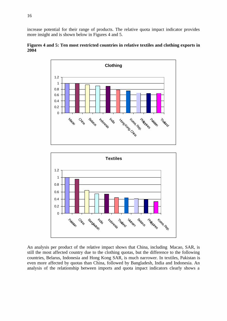
increase potential for their range of products. The relative quota impact indicator provides more insight and is shown below in Figures 4 and 5. Figures 4 and 5: Ten most restricted countries in relative textiles and clothing exports in 2004

Clothing

0

0.2

0.4

0.6

0.8

1

1.2

MacaoChina

Belarus

Indonesia

IndiaHong Kong, China

Korea, Rep.

Philippines

Pakistan

Thailand

Textiles

0

0.2

0.4

0.6

0.8

1

1.2

Pakistan

ChinaBangladesh

IndiaIndonesia

Thailand

Vietnam

Belarus

Philippines

Korea, Rep.

An analysis per product of the relative impact shows that China, including Macao, SAR, is still the most affected country due to the clothing quotas, but the difference to the following countries, Belarus, Indonesia and Hong Kong SAR, is much narrower. In textiles, Pakistan is even more affected by quotas than China, followed by Bangladesh, India and Indonesia. An analysis of the relationship between imports and quota impact indicators clearly shows a

17

positive correlation. 9. In other words, quotas are specifically targeted to countries who could export on a large scale and who have, therefore, the potential to serve a large market. 4.2. A gravity model approach to forecast trade shifts 4.2.1. The model Now that we have constructed a quota indicator for both aggregates textile and clothing, we can use it to analyse the impact of the quotas on trade by using the gravity model. The first gravity models were simply cross-section regressions, using one year and a limited amount of countries or regions. Due to increased data availability, econometrical knowledge and calculating capacity, more sophisticated versions have been developed. These versions use the availability of time series and the development in panel data modelling, leading to more efficient and accurate estimates due to the increased amount of data and inclusion of the information given by the time structure (Verbeek, 2002). We now discuss the gravity model characteristics. Gravity model principle As mentioned, the gravity model takes its name from the Newtonian principle that masses attract. Empirical investigations in international trade using the gravity equation typically note that formal theoretical foundations for the model have been provided in Anderson (1979), Krugman (1979), Helpman, Elhanan and Krugman (1985),10 Bergstrand (1985, 1989, 1990), and van Wincoop and Anderson (2003) and are now well established. In these studies, the gravity equation is derived theoretically as a reduced form from a general equilibrium model of international trade in final goods. Exporter and importer GDPs can be interpreted in these models as the production and absorption capacities of the exporting and importing countries, respectively. Bilateral distance between the two countries is generally associated with transportation costs; more distance suggests greater transit costs.11 Gravity equation The basic formulation of the gravity equation for imports is as follows:

ijteXI ijtijtεβα= (3)

where ijtI is the import in country i from country j at time t, α is the constant, X are the

explanatory variables and ε is the error term with expectation zero and variance εσ . The model can be transformed into a linear equation by taking the natural logarithm on both sides, which gives:

9 Correlation value of 0.49 for textiles and 0.22 for clothing at a 0.01 significance level for the 1999 – 2004 period 10 Baldwin (1994) noted that, ‘The gravity model used to have a poor reputation among reputable economists. Starting with Wang and Winters (1991), it has come back into fashion. One problem that lowered its respectability was its oft -asserted lack of theoretical foundations. In contrast to popular belief, it does have such foundations.’ (p. 82). 11 As many authors have noted, the ‘costs’ of distance may extend well beyond freight charges, including cultural dissimilarities and other barriers measured with difficulty (cf., Anderson, 1999). Thus, while distance has always been an important variable in gravity equations, authors have never been sure exactly what ‘costs’ distance represents.

18

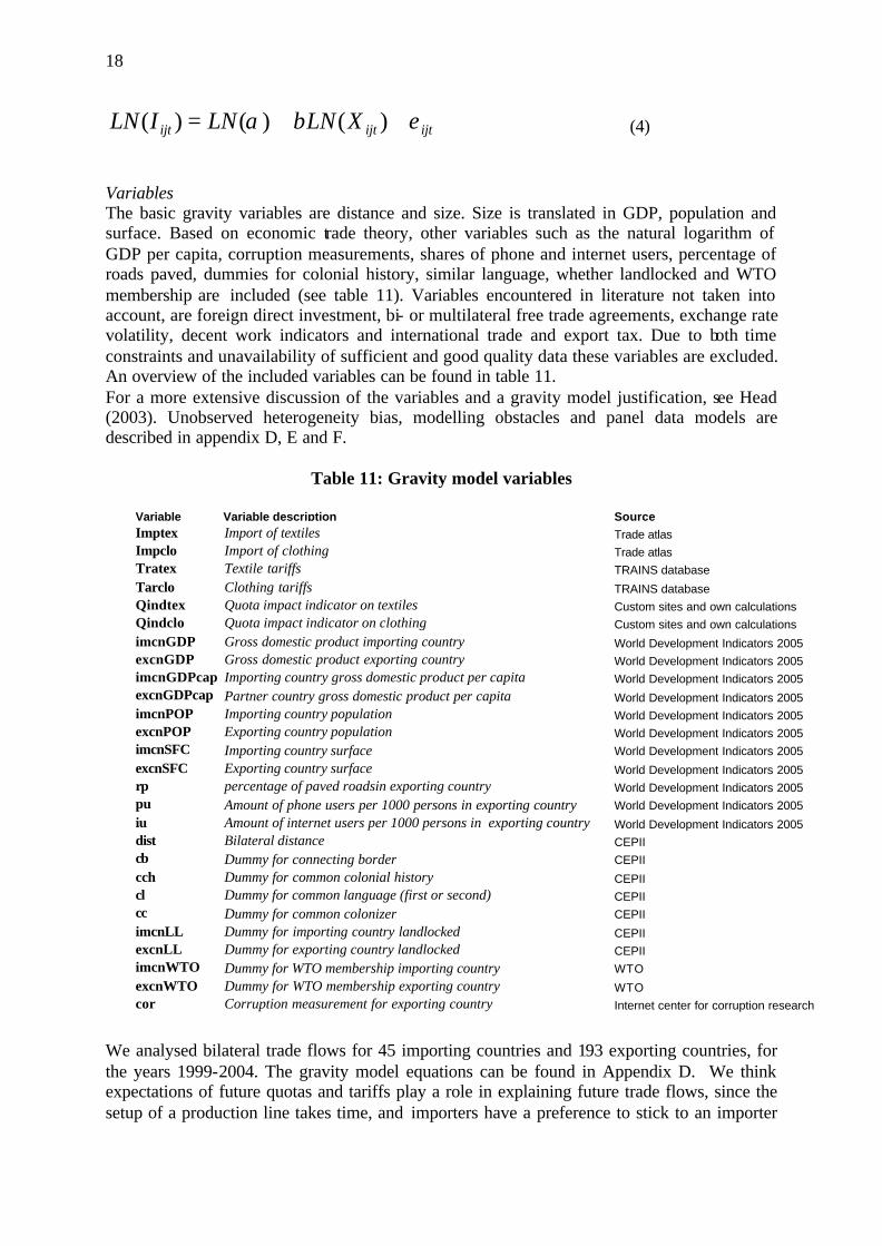
ijtijtijt XLNLNILN εβα ++= )()()( (4) Variables The basic gravity variables are distance and size. Size is translated in GDP, population and surface. Based on economic trade theory, other variables such as the natural logarithm of GDP per capita, corruption measurements, shares of phone and internet users, percentage of roads paved, dummies for colonial history, similar language, whether landlocked and WTO membership are included (see table 11). Variables encountered in literature not taken into account, are foreign direct investment, bi- or multilateral free trade agreements, exchange rate volatility, decent work indicators and international trade and export tax. Due to both time constraints and unavailability of sufficient and good quality data these variables are excluded. An overview of the included variables can be found in table 11. For a more extensive discussion of the variables and a gravity model justification, see Head (2003). Unobserved heterogeneity bias, modelling obstacles and panel data models are described in appendix D, E and F.

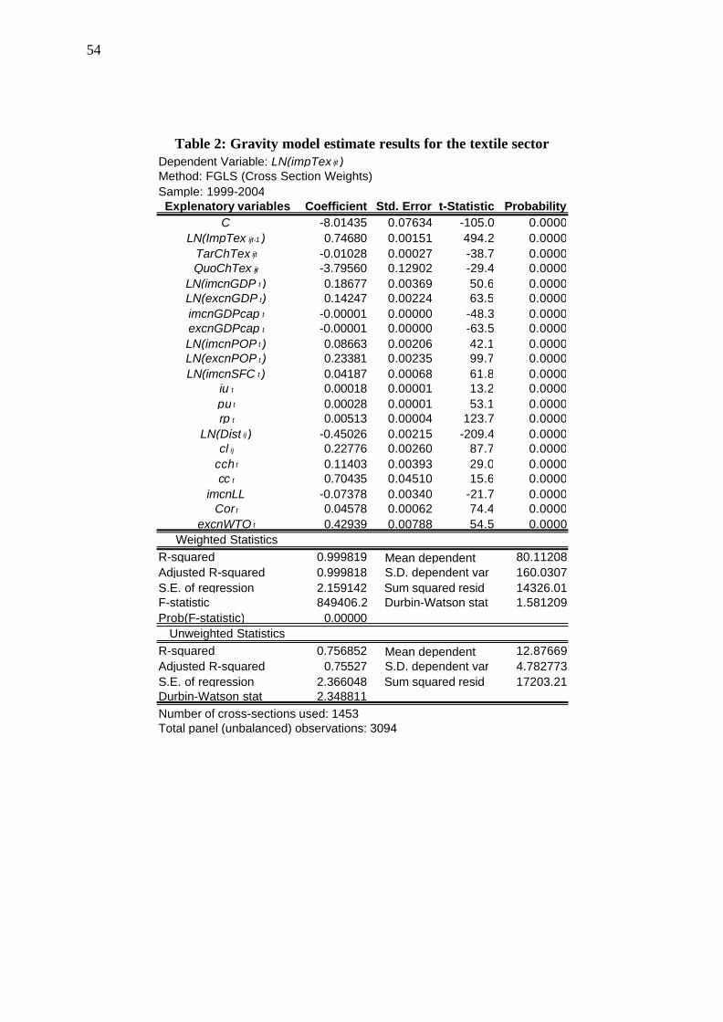
Table 11: Gravity model variables We analysed bilateral trade flows for 45 importing countries and 193 exporting countries, for the years 1999-2004. The gravity model equations can be found in Appendix D. We think expectations of future quotas and tariffs play a role in explaining future trade flows, since the setup of a production line takes time, and importers have a preference to stick to an importer

Variable Variable description SourceImptex Import of textiles Trade atlasImpclo Import of clothing Trade atlasTratex Textile tariffs TRAINS databaseTarclo Clothing tariffs TRAINS databaseQindtex Quota impact indicator on textiles Custom sites and own calculationsQindclo Quota impact indicator on clothing Custom sites and own calculationsimcnGDP Gross domestic product importing country World Development Indicators 2005excnGDP Gross domestic product exporting country World Development Indicators 2005imcnGDPcap Importing country gross domestic product per capita World Development Indicators 2005excnGDPcap Partner country gross domestic product per capita World Development Indicators 2005imcnPOP Importing country population World Development Indicators 2005excnPOP Exporting country population World Development Indicators 2005imcnSFC Importing country surface World Development Indicators 2005excnSFC Exporting country surface World Development Indicators 2005rp percentage of paved roadsin exporting country World Development Indicators 2005pu Amount of phone users per 1000 persons in exporting country World Development Indicators 2005iu Amount of internet users per 1000 persons in exporting country World Development Indicators 2005dist Bilateral distance CEPIIcb Dummy for connecting border CEPIIcch Dummy for common colonial history CEPIIcl Dummy for common language (first or second) CEPIIcc Dummy for common colonizer CEPIIimcnLL Dummy for importing country landlocked CEPIIexcnLL Dummy for exporting country landlocked CEPIIimcnWTO Dummy for WTO membership importing country WTOexcnWTO Dummy for WTO membership exporting country WTOcor Corruption measurement for exporting country Internet center for corruption research

19

they know since to change wastes resources, therefore, when importers invest in a production line it has to have good prospects, and they use their expectations on future trade regimes to determine their orders. Therefore, we believe that not only the quota strictness and the tariff in the year itself matters, but also the expectation of change in the quota strictness and the tariffs for the following year influences imports of the current year. Hence, we constructed an indicator in which we use the quota impact indicator and the tariff of the year t + 1 as an instrument for the expectation of the quota strictness and the tariff of the following year. We take the one-year difference so we have the expected change in quota strictness, and in the quota case we divide by the maximum to normalize. The interpretation of the β3 estimate should be: A change of 1 between today’s quota strictness and the expected quota strictness in the next year influences the LN(impX) of today with β3 . We use β3 to forecast. Under the new quota regime the quota indicator has a value of zero for all countries. Therefore, we take the difference between the last year of the quota (2004) and zero. We multiply β3 by this number and add half the variance of the disturbance term to find an estimate for LN(impXijt+). We take the exponent and normalize for constant demand to estimate future imports. First we execute a FGLS estimation approach, with White standard errors. Then we use a general to specific approach and eliminate insignificant variables. To test for autocorrelation in a model with a lagged dependent variable we use the Breusch-Godfrey Langrange Multiplier test for autocorrelation, which is constructed as T times the R² of a regression of the least square residuals at moment t on the least square residuals of moment t-1 and all other explanatory variables (including the lagged dependent). The test statistic should have Chi-squared distribution with 1 degree of freedom. The estimation results and B-G LM tests for autocorrelation can be found in the Attachment, Tables la, lb and 2. For both models the B-G LM tests do not give us reason to reject the null hypothesis of no autocorrelation. This means that the estimators should be consistent. Forecast assumptions This paper does not extensively discuss or compare the gravity model results for the other variables in the model. What we can say is that they have the same sign, but for most variables a magnitude closer to zero. This might be due to special characteristics of the trade in textiles and clothing. However, in order to make forecasts we are mainly interested in the parameter estimate of β3 , the magnitude of the quota impact indicator. Before making any forecasts it is important to know how to interpret the results, since they are done under the ceteris paribus assumption, which is a very strong assumption in a dynamic environment. There are many important factors for which the ceteris paribus assumption is arguable; a few important factors are discussed below.

- Constant demand: the demand in value in textiles and clothing will not change in any region. This assumption excludes a decline or increase in value demand due to a change in prices or global demand growth.

o We expect a lowering of prices due to the ATC phase out, but the effects on total demand are unclear. However, when clothing and textiles are considered primary instead of luxury goods, the price elasticity is probably lower then one so value demand should decrease in case of lower prices.

o We expect a global demand growth, especially due to the growth of the South Asian countries. An increased global demand might absorb and compensate for export losses in different countries.

20

- Production limits: Countries are not able to increase their production limitlessly without increasing cost; the forecast however assumes infinite production expanding capacity and non-changing cost. A big part of the trade redistribution depends on the production capacity limit and the production cost elasticity in China, which is unknown today.

- ATC phase out preparation: Countries that were benefiting from the ATC and had, therefore, no sufficient motivation to improve their production processes might have been preparing for the ATC phase out. They may have become more competitive, thereby retaining their market share.

- Re-imposing of quotas: The US and EU have already imposed new quotas on the imports from China. The forecast assumes a trade regime without quotas, and even without expectation of new quotas. Due to the re- imposing of the quotas the forecasts will not be valid for today, but should be interpreted as a general direction in which the new trade distribution is moving after the expected fadeout of the re- imposed quotas after 2008.

- Shift to higher value added products: For different South Asian countries, which were restricted by the quotas, we observe a declining trend in exports in T&C due to an increase in the export of higher value added products. This decreasing trend in T&C has not been taken into account, but it is nevertheless important.

- Currency devaluation: Countries with a large export share in T&C, might experience a devaluation due to less demand for local currency. This devaluation lowers prices and may in part recover demand, although never to its former level. This effect has, however, not been taken into account.

There are many other factors that influence trade, but have not been accounted for. Examples are destabilizing factors such as war or terrorist threats, financial crisis, natural disasters, etc. Taking these uncertain factors into account, the results should be interpreted as a general direction in which the new trade distribution in T&C is moving. 4.2.2. Trade results As already mentioned, we distinguish between textiles and clothing, but we also look into the different effects on exports towards the US and EU and the effects on total trade also include Canada. Clothing First we look at the trade change from the perspective of the quota imposing countries. From which countries can they expect an import increase?

21

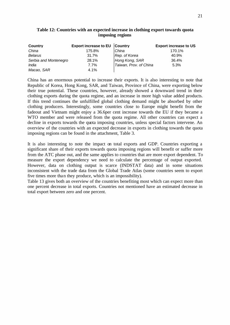
Table 12: Countries with an expected increase in clothing export towards quota imposing regions

Country Export increase to EU Country Export increase to USChina 175.8% China 170.1%Belarus 31.7% Rep. of Korea 40.9%Serbia and Montenegro 28.1% Hong Kong, SAR 36.4%India 7.7% Taiwan, Prov. of China 5.3%Macao, SAR 4.1%

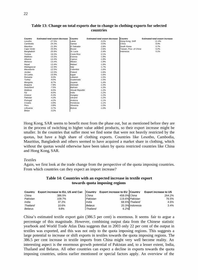
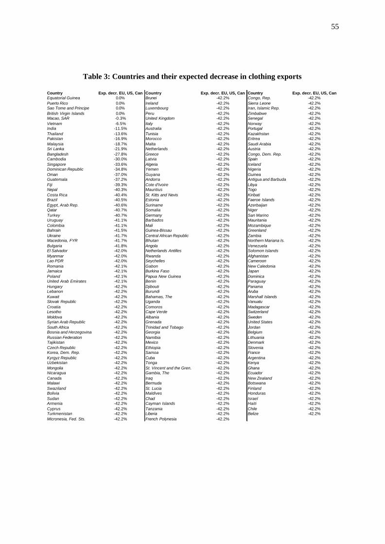
China has an enormous potential to increase their exports. It is also interesting to note that Republic of Korea, Hong Kong, SAR, and Taiwan, Province of China, were exporting below their true potential. These countries, however, already showed a downward trend in their clothing exports during the quota regime, and an increase in more high value added products. If this trend continues the unfulfilled global clothing demand might be absorbed by other clothing producers. Interestingly, some countries close to Europe might benefit from the fadeout and Vietnam might enjoy a 36.6per cent increase towards the EU if they became a WTO member and were released from the quota regime. All other countries can expect a decline in exports towards the quota imposing countries, unless special factors intervene. An overview of the countries with an expected decrease in exports in clothing towards the quota imposing regions can be found in the attachment, Table 3. It is also interesting to note the impact on total exports and GDP. Countries exporting a significant share of their exports towards quota imposing regions will benefit or suffer more from the ATC phase out, and the same applies to countries that are more export dependent. To measure the export dependency we need to calculate the percentage of output exported. However, data on clothing output is scarce (INDSTAT data) and in some situations inconsistent with the trade data from the Global Trade Atlas (some countries seem to export five times more than they produce, which is an impossibility). Table 13 gives both an overview of the countries benefiting most which can expect more than one percent decrease in total exports. Countries not mentioned have an estimated decrease in total export between zero and one percent.

22

Table 13: Change on total exports due to change in clothing exports for selected countries

Country Estimated total export decrease Country Estimated total export decrease Country Estimated total export increaseLesotho -27.5% Latvia -3.2% Hong Kong, SAR 11.4%Cambodia -24.3% Samoa -3.0% China 8.4%Mauritius -21.9% El Salvador -2.8% South Korea 0.7%Cape Verde -20.9% Brunei -2.6% Taiwan, Prov. of China 0.2%Bangladesh -20.9% St. Lucia -2.4% Indonesia 0.1%Tunisia -16.5% Costa Rica -2.1%Maldives -15.5% Estonia -1.9%Albania -14.4% Cyprus -1.9%Morocco -13.4% Mexico -1.9%Nepal -13.4% Malawi -1.9%Madagascar -12.9% Italy -1.7%Macedonia -12.5% Colombia -1.6%Jordan -12.0% Poland -1.6%Sri Lanka -10.9% Egypt. -1.6%Romania -9.3% Lebanon -1.5%Turkey -9.0% Guatemala -1.5%Mongolia -8.7% Guyana -1.4%Bulgaria -7.8% Denmark -1.3%Swaziland -7.5% Bahrain -1.3%Moldova -6.5% Slovak Republic -1.2%Fiji -6.0% India -1.2%Greece -5.4% Hungary -1.2%Pakistan -4.3% Ukraine -1.2%Portugal -4.2% Andorra -1.1%Croatia -3.9% Honduras -1.1%Peru -3.8% Slovenia -1.0%Lithuania -3.7% Bolivia -1.0%Belize -3.2% Hong Kong, SAR seems to benefit most from the phase out, but as mentioned before they are in the process of switching to higher value added products, so their export increase might be smaller. In the countries that suffer most we find some that were not heavily restricted by the quotas, but have a high share of clothing exports. Countries like Lesotho, Cambodia, Mauritius, Bangladesh and others seemed to have acquired a market share in clothing, which without the quotas would otherwise have been taken by quota restricted countries like China and Hong Kong, SAR. Textiles Again, we first look at the trade change from the perspective of the quota imposing countries. From which countries can they expect an import increase?

Table 14: Countries with an expected increase in textile export towards quota imposing regions

Country Export increase to EU, US and Can Country Export increase to EU Country Export increase to USChina 386.5% China 458.0% China 264.2%Pakistan 109.7% Pakistan 119.6% Pakistan 76.5%India 37.2% India 68.6% Thailand 4.6%Thailand 10.6% Belarus 20.3% Indonesia 3.4%Belarus 9.8% Thailand 6.2% China’s estimated textile export gain (386.5 per cent) is enormous. It seems fair to argue a percentage of this magnitude. However, combining output data from the Chinese statistic yearbook and World Trade Atlas Data suggests that in 2003 only 22 per cent of the output in textiles was exported, and this was not only to the quota imposing regions. This suggests a large potential to increase or shift exports in textiles towards the quota imposing regions. The 386.5 per cent increase in textile imports from China might very well become reality. An interesting aspect is the enormous growth potential of Pakistan and, to a lesser extent, India, Thailand and Belarus. All other countries can expect a decline in exports towards the quota imposing countries, unless earlier mentioned or special factors apply. An overview of the

23

countries with an expected decrease in exports in textiles towards the quota imposing regions can be found in the Attachment, Table 4. To get a more realistic view of the true impact, we again look at the effect on total exports, since this gives us more insight into the countries that are most affected in practise due to their greater export dependence on textiles.

Table 15: Effect on total exports due to change in textile exports

Country Estimated total export decrease Country Estimated total export decrease Country Estimated total export increaseNepal -4.5% Luxembourg -1.2% Pakistan 23.1%Turkey -2.4% Uruguay -1.2% China 4.8%Egypt -2.4% Bangladesh -1.1% India 2.1%Niger -2.2% Gambia -1.1% Belarus 0.3%Lesotho -1.9% Mongolia -1.1% Thailand 0.1%Burkina Faso -1.7% Lithuania -1.1%Portugal -1.6% Estonia -1.0%Greece -1.4% Tunisia -1.0%Syria -1.3% Benin -1.0%Uganda -1.2% Italy -1.0% The effect on the total exports of Pakistan could be enormous because they have a high share of textile exports (48 per cent) and under the ATC regime around 44 per cent of their textile exports went to quota imposing regions. For China an export gain of 4.8 per cent is quite substantial, as it would be for countries like Nepal, Turkey and Egypt that could see their exports decrease from 2.4 per cent to 4.5 per cent. Total To see the effect on a country’s total export due to the ATC phase-out, we look at the total impact on exports. The countries that might potentially gain are found on the right, and the corresponding percentage is the estimated increase in the countries total exports in all products.

Table 16: Total effect on exports of the ATC phase-out

Country Total export decrease Country Total export increaseLesotho -29.4% Pakistan 18.8%Cambodia -24.5% China 13.2%Mauritius -22.2% Hong Kong, SAR 11.3%Bangladesh -22.0% India 0.9%Nepal -17.9% Korea, Rep. 0.6%Tunisia -17.5% Belarus 0.3%Maldives -15.5% Taiwan, Prov. of China 0.1%Albania -14.6%Morocco -13.9%Madagascar -13.5%Macedonia -13.2%Jordan -12.2%Sri Lanka -11.6%Turkey -11.4%Romania -10.0%

24

Beneficiaries again include countries like Pakistan, China and Hong Kong, SAR. If we consider that Hong Kong, SAR is an export heaven for China, the total export increase for China might be even larger than suggested in Table 16. Pakistan has such a high percentage of estimated increase due to its expected high increase in textiles, but with an expected loss of market share in clothing. The countries where we estimate contracting exports are those that enjoyed preferential treatment before the ATC phase-out, but now face harder competition. The countries shown in Table 16 are those that are estimated to have a more than then 10 per decrease in total exports. Other countries can be found in the Attachment, Table 5. 4.3. Trade shifts and their impact on employment 4.3.1. Calculation of the link between trade and employment In order to estimate the effect of a change in exports on employment, we need to define the relationship between the two. Under the ceteris paribus assumption, a change in exports should lead to a change in output, and therefore a change in employment. The relative magnitude of the change in output as a result of a change in exports depends on the fraction of output being exported. The change in output is then:

XOX

O ∆=∆ (8)

where O is output, X is exports and ∆ represents change. This formula assumes constant demand within the country. To determine the change in employment, we need to know what the employment elasticity of output is. We estimate this by running the following regression.

εβα ++= )()( OLNELN (9) where )(ELN is the natural logarithm of employment, )(OLN is the natural logarithm of output, α is a constant and ε is an error term with expectation zero and variance εσ . We can interpret the estimate of β as the employment elasticity of output, which we can see when we

take equation 9 and calculate the derivative for both sides, and solving for∂∂EY

:

1E

EY

YEY

EY

=

⇒ =

∂

β∂

∂∂

β (10)

We see here that ß represents the magnitude in change in employment due to a change in output. Results For the regression we use UNIDO output and employment data from the years 2001, 2000 and 1996 and we distinguish between textile and clothing and industrialized and non-industrialized countries. The estimated ßs can be found in Table 17 below.

25

Table 17: Employment/output elasticities

Textile ClothingIndustrialized 0.47 0.49Non-industrialized 0.51 0.52

However, since the employment and output data are from a period devoid of big global shocks, the estimates are valid for small shocks; when there is a decrease in output of 1 per cent, there is a decrease in employment of approximately 0.5 per cent. However, in the case of a big shock, when there is an output decline of 100 per cent, the employment must also decrease by 100 per cent. In order to deal with big shocks, we use some assumptions:

- we assume the employment elasticity is valid for the average output change; - for big output changes we assume the pattern is logarithmic and results in a 100 per

cent employment decline when output declines by 100 per cent. Then the transformation function resembles the following:

1/))11

)(1(1( −−∆++=∆ COLNLijβ

(11)

where L∆ = the percentage of labour change, and O∆ is the percentage in output change. The C is a constant to assure that the function gives a -100 per cent labour change for a -100 per cent output change. In a graph the situation looks like the following, where 0 is the initial employment rate, which is considered 100 per cent.

Figure 6: Output –employment relationship

26

Using the transformation function, an output decline of 100 per cent will lead to an employment decline of 100 per cent and for small changes the employment-output elasticity still holds approximately. 4.3.2. Results As previously mentioned, in order to use the estimated labour shift to make a reasonable estimate on future labour shifts, we need to know the initial number of workers and the export/output relationship. Unfortunately, data on both employment and output on the T&C level is scarce. The countries for which all data was available are noted below in Table 18.

Table 18: Countries for which data is available in order to estimate labour shifts in clothing

Country Nr of employees Export fraction Change in jobs Country Nr of employees Export fraction Change in jobsCanada 105017 0.42 -14451 China 11521433 0.22 1204163Brazil 813862 0.06 -12896 India 1182123 0.31 52554Switzerland 6299 0.77 -1578 Indonesia 618878 0.57 -3407Japan 240993 0.05 -1307 Romania 91400 0.31 -5978Ecuador 9137 0.37 -848 Morocco 41303 0.18 -1779Cyprus 2603 0.47 -414 Malaysia 40200 0.65 -1201Norway 1663 0.64 -335 Bulgaria 34047 0.61 -3755

Clothing Textile

The number of employees in the textile sector in China is an estimate, since we only have the total number of employees in textile and clothing. This estimate is based on output numbers and general labour intensity in both sectors. For the clothing sector we have no reliable data for the export fraction, so we cannot calculate a labour shift. For other countries we use the average export fraction of 0.42 for textiles and 0.32 for clothing and use these to estimate an expected labour shift. The results are in the Attachment, Table 5. Most countries either gain or lose in both categories, but there are a few countries where we expect a labour gain in textiles, and a loss in clothing and vice versa. Examples are Pakistan, India, Indonesia and the Philippines. These countries may solve an unemployment loss in one sector by an employment gain in the other. A total labour impact analysis follows below Total We calculate total expected labour shifts using the average export fraction. For some countries the export fraction might be different in reality, but due to the lack of data this is the best we can do. Table 19 lists the countries for which we can calculate an estimated labour increase.

Table 19: Countries with estimated job gain

Country Number of extra jobsChina 2130609Pakistan 213635India 40684

Hong Kong, SAR, South Korea, Belarus and Taiwan, Province of China, would also have an estimated labour increase, but we do not have reliable labour data. The increase of jobs in China is equal to approximately an 11 per cent increase of the 19 million workers in the T&C

27

industry in China, and for Pakistan the number means an increase of around 12 per cent of the approximately 2.55 million workers in Pakistan.

Table 20: Estimated effect of the ATC phase out on employment

Country Total inpact on employment Country Total inpact on employment Country Total inpact on employmentBangladesh -221084 Vietnam -9387 Jordan -1324Cambodia -78779 Germany -9172 Japan -1307Romania -48359 Hungary -8738 Israel -1213Italy -36502 Mauritius -8605 Botswana -993Turkey -35043 Colombia -7348 Ecuador -848Poland -26746 Thailand -7230 Austria -826Morocco -20861 Argentina -5477 Tanzania -807Tunisia -20518 Malaysia -4234 Guatemala -768Portugal -20442 Lithuania -4135 Finland -719Bulgaria -18808 Croatia -4111 Ireland -703Spain -18101 Algeria -2747 Singapore -690Madagascar -16906 Greece -2702 Albania -668South Africa -14946 Nepal -2024 Sweden -662Canada -14451 Kenya -1651 El Salvador -648Sri Lanka -12896 Switzerland -1578 Denmark -615Brazil -12896 Indonesia -1555 Cyprus -575France -11729 Latvia -1420 Uruguay -561 The numbers are estimates so should be interpreted solely as indicative of future labour shifts. Of particular concern are future labour shifts that might occur in the developing and transitional economies of Bangladesh, Cambodia, Romania, Poland and Turkey, where the T&C industry holds a prominent position and, therefore, involves many jobs. However, recent developments in Cambodia indicate that labour loss might be less severe since a few major European and US brands (e.g. GAP) have confirmed, according to a World Bank Survey of textile and garment buyers sourcing in Cambodia, that they will continue to order from Cambodia due to the presence of the ILO which is monitoring and securing decent working conditions. This is important since, according to the major importers, consumers take decent working conditions into account when making their consumption decisions. The magnitude of labour loss in developed countries such as Italy, Portugal and Canada is substantial with around 15-35,000 jobs being lost. In summary, we cannot say whether there is a global labour gain or loss, since we do not have labour data for about half the countries. However, since the total labour gain in the countries where we have data is less than one million, and for China there is an expected gain of more than two million, we can expect a total global job gain, but this almost entirely due to the Chinese.

5. Conclusion The T&C industry is considered to be an opportunity and a first step for the industrialization of developing countries in low value added manufacturing goods. The phasing out of the MFA will mean a strong reduction of distortions to trade in textiles and clothing and more transparency, even though the recent reinstallation of safeguard measures in the USA and the EU temporarily hampers this evolution. Moreover, tariffs will become a major trade hurdle for exporting countries, together with other non tariff trade barriers such as eco- labels. Overall, the end of the MFA will reshape the T&C industry in terms of trade, production and employment, providing new business opportunities, but also bringing economic and social threats. In general, clothing, and even more so textiles, are less sophisticated low-value goods.

28

They are labour- intensive and thus need a large number of unskilled workers, including a high share of female workers. There has been a general decline in employment in this industry as a result of a consolidation and rationalization process. OECD countries have been pulling out of the sector or have been surviving in specific niches, where they have increased the use of capital, generating a strong productivity rise. Exports went up steeply in South-East and South Asia. The emergence of new producers in Africa and Central America, benefiting from preferential access to rich markets, was also striking. In absolute values, worldwide, employment in textiles and clothing employment is important, in particular in China, as well as in Pakistan, Bangladesh and India. Nevertheless, this industry is often very important in relative terms in many developing countries such as Mauritius, Madagascar and Cambodia as the share of T&C employment in total manufacturing employment is extremely high. The analysis of the trade competitiveness situation, as well as the forecast of the gravity model, shows that the phasing out implies significant changes in the worldwide trade structure, leading to strong output and employment shifts in and between countries. First, clear winners of this new era will emerge. China and Pakistan will be the biggest winners according to our forecast, as well as China, including Hong Kong, SAR, and Macao, SAR in general and Taiwan, Province of China, South Asian countries (e.g. India) and Belarus. There will then be the countries which are “slight” losers, but could be potential winners if they apply the right policies. The restructuring and modernization of their production, the creation of political or enterprise alliances with leading companies and countries and the integration into global production systems are key questions in this regard. Within this group, you can find some smaller countries with good transport connections and low labour costs in South and South-East Asia, such as Thailand, Cambodia and Bangladesh. They could integrate their domestic production into the production systems of the successful countries of the region. Third, there are the loser countries, losing part, even large parts, of their T&C industry, but which may have the capacity to survive in niches, applying specific restructuring strategies. Countries like Mexico and perhaps other Central American States, benefiting from their proximity to the US market could come under this category, but also important European producers like Germany, which already restructured its industry to specialize in specific high quality segments in order to face higher world competition. Countries that might benefit from niches due to their proximity to the EU market are Romania, Turkey, Morocco and Egypt. There is a fourth category of countries that will lose out completely in T&C and have to diversify their economy and find other sectors of industrial specialization. On the one hand, you have smaller OECD countries, which may have the capacity to reorientate national production towards other sectors, and on the other hand, you have small and less developed countries previously benefiting from privileged access to the US and EU markets. Sub-Saharan countries such as Lesotho or Madagascar may belong to this group. The phasing out of the MFA implies employment churning and shifts in all four groups of countries, as a result of positive or negative changes in production. Developing countries from group three and four, which will partially or totally lose production, and thus employment are at the centre of our concern. A fast adjustment of production to the new situation and a combination of active and passive labour market policies for workers during the transition period may be necessary to reduce the social cost of adjustment. Workers may have to be retrained for other sectors and may need financial support for the transition period. It will be crucial to effectively combine industrial with labour market policies. In extreme cases, the affected country will completely lose its T&C production and thus have to diversify its economy, looking for new areas of specialization. Recent strategies of diversification applied

29

by Mauritius may give interesting indications for similar African countries or smaller Central American countries. The international community also has a responsibility to help the most disadvantaged countries, especially those that do not have sufficient technical and financial capacities to adjust to the new situation. International financial institutions, private and public donors from countries, in particular those where consumers benefit most from the new situation, USA and EU, or even “winning” developing countries from South and South-East Asia, could create a “solidarity” fund to help the most affected countries in their restructuring process. This assistance could be combined with the concession of trade privileges in other sectors that may be developed during the restructuring process (e.g. light manufacturing, food, mining processing, business services or tourism), or by public support and by private initiatives to integrate new productive activities into global produc tion systems. These measures could help avoid future trade conflicts, reduce social hardship and contribute to a more equitable share of the welfare benefits in T&C trade.

30

31

BIBLIOGRAPHY Anderson, James E (1979): A Theoretical Foundation for the Gravity Equation, American Economic Review, American Economic Association, vol. 69(1), pages 106-16. Anderson, James E (1999): “Why Do Nations Trade (So Little)?,” Boston College Working Papers in Economics 428, Boston College Department of Economics. Anderson, James and van Wincoop, Eric (2004): “Trade Costs”, Journal of Economic Literature, Volume XLII (September 2004) pp 691-751 Appelbaum, Richard P., 2004: Assessing t he Impact of the Phasing-out of the Agreement on Textiles and Clothing on Apparel Exports on the Least Developed and Developing Countries, in Global & International Studies Program, Paper 33, University of California, Santa Barbara. Baldwin, R. (1994), Towards an integrated Europe (CEPR, London). Bayoumi, Tamim, and Eichengreen, Barry (1997) “Is regionalism Simply a Diversion?” Evidence from the evolution of the EC amd EFTA.” In regionalism vs Multilateral Arrangements, edited by Takatoshi Ito and Anne O. Kreuger. Chicago: The university of Chicago press, 1997 Bergstrand, Jeffrey H, (1989). "The Generalized Gravity Equation, Monopolistic Competition, and the Factor-Proportions Theory in International Trade," The Review of Economics and Statistics, MIT Press, vol. 71(1), pages 143-53. Bergstrand, Jeffrey H, (1990). "The Heckscher-Ohlin-Samuelson Model, the Linder Hypothesis and the Determinants of Bilateral Intra- industry Trade," Economic Journal, Royal Economic Society, vol. 100(403), pages 1216-29. Deardorff, Alan V. (1995), "Determinants of Bilateral Trade: Does Gravity Work in a Neoclassical World?," NBER Working Papers 5377, National Bureau of Economic Research, Inc. Dussel Peters , Enrique (2004): Oportunidades y retos económicos de China para México y Centroamérica, ECLAC, Working Paper, LC/MEX/L.633, 27 September 2004, Mexico. Frankel, Jeffrey A. (1997), Regional trading blocs in the World Economic System, chapter 4, the Gravity model of bilateral trade. Head, Keith (2003): “Gravity for beginners” University of British Colombia, Vancouver. Helpman, Elhanan and Krugman, Paul R. (1985) Market Structure and Foreign Trade. Cambridge: MIT Press. Hightower, Neil (2004): Comparison of the Textile Industry in Mexico and China, Asamblea Annual de Canaintex, March, México. Institut Français de la Mode (2004): Study on the Implications of the 2005 Trade Liberalisation in the Textile and Clothing Sector, Consolidated Report, Paris.

32

Kyvik Nord?s, Hildegunn (2004): Labour Implications of the Textiles and Clothing Quota Phase-Out, Working Paper No.224, Sectoral Activities Department, ILO, Geneva. Krugman, Paul R. (1979) “Increasing Returns, Monopolistic Competition and International Trade.” Journal of International Economics 9:469-79. Lankes, H.P., (2002), “Market Acces for Developing Country Exports”, Finance and Development (September 2002), pp 8 – 13. Mohamed Hedi Bchir & Yvan Decreux & Jean-Louis Guerin & Sebastien Jean (2002) "MIRAGE, un modele d'equilibre general calculable pour l'evaluation des politiques commerciales," Economie Internationale, CEPII research center, issue 1T-2T, pages 109-153. Newspapers : China Daily, Emerging Textiles, The Dawn, The Independent. Oguledo, Victor Iwuagwu & MacPhee, Craig R (1994), "Gravity Models: A Reformulation and an Application to Discriminatory Trade Arrangements” Organisation for Economic Co-Operation and Development (OECD), (2004): A New World Map in Textiles and Clothing, Adjusting to Change. Tinbergen, Jan (1962): Shaping the World Economy. New York: The Twentieth Century Fund, 1962 Verbeek, Marno (2002): a guide to modern econometrics. Wang, Zhen K. and Alan L. Winters (1991) "The Trading Potential of Eastern Europe". London: CEPR Discussion Paper, No. 610. Wooldridge, Jeffrey M. (2002): Econometric analyses of cross section and panel data.

33

DATA SOURCES BMGEA: Bangladesh Garment and Manufacturers Association. CEPII: Centre d’Etudes Prospectives et d’Informations Internationales EPB (Export Promotion Board), Bangladesh. Cambodia: Industry of Commerce. China Ministry of Commerce MOFCOM. China, Statistical Yearbook 2005. Federal Bureau of Statistics of Pakistan. Global Trade Atlas. Guatemala: Asociación Gremial de exportadores de productos no tradicionales. ITC, Trade Map (http://www.intracen.org/mas/trade.htm) and Countries (http://www.intracen.org/menus/countries.htm). INE (Instituto Nacional de Estadística), Guatemala. Madagascar: Labour and Social Law Ministry. Mexico: National Chamber of Textile Industry. OECD, Labour Market Statistics. UN COMTRADE. UNCTAD TRAINS database. UNDP, Human Development Indicators 2004. UNIDO, Indstat, Rev. 3 and 2, 2003 and 2005. US Department of Commerce/OTEXA. European commission of trade, SIGL International Trade Canada. World Bank, World Development Indicators 2005. World Trade Organisation www.icgg.org

34

35

Appendix A Table 1: World market share and its evolution in textiles and clothing, 1999-2003 Countries

% in WMS % annual change in WMS % in WMS % annual change in WMSChina 21,59% 5'29% 14'92% 11'61%Bangladesh 2'58% 1'35% 0'25% 0'71%India 2'74% -2.52% 3'79 0'13%Pakistan 1'08% 0'90% 2'56% 0'65%Sri Lanka 1'10% -3.41% 0'08% -9.64%Nepal 0'08% -10.98% 0'09% -7.16%Morocco 1'34% 2'73% 0'08% -0.68%Mauritius 0'41% -2.94% 0'04% -6.92%Madagascar 0'10% -9.17% 0'01% -13.25%Mexico 3'04% -6.85% 1'16% -6.17%Guatemala 0'04% 21,58% 0'03% 1'92%Romania 1'69% 11'57% 0'24% 19'70%Turkey 4'13% 7'21% 2'91% 6'44%

Clothing Textiles

Note: WMS = World Market Share. Source: ITC, Countries and Trade Map. A closer look at the share of each country in the world market (Table 4) demonstrates the dominant position of China even before 2005, with the highest share in textiles and clothing. Its position was especially hegemonic in the clothing industry, with one-fifth of the world share between 1999 and 2003. China even increased its share by 5.3 per cent in the clothing sector during these four years. Several countries have suffered a remarkable fall in their share, even in both sectors, for example, Sri Lanka, Nepal, Madagascar and Mexico. In contrast, there were some countries that experienced a considerable rise in their world market share. This was the case of some European countries, like Turkey and Romania, but also Guatemala, which achieved the highest growth (21.6 per cent) in world market share in clothing, although its share in the world market was still insignificant (0.04 per cent).

36

Table 2: Trend of exports and change in competitiveness in clothing and textiles, 1999-2003

Countries Change in competitivenessClothing Textiles Clothing Textiles

China 10% 19% 4'31% 9'01%Bangladesh 6% 7% 1'14% 1'02%India 4% 8% -2.44% 1'31%Pakistan 8% 6% 0'28% 0'99%Sri Lanka 3% 9% -1.70% -7.55%Nepal -4% 4% -9.47% -2.31%Morocco 9% 58% -1.95% 0'29%Mauritius 3% 70% -3.82% -6.22%Madagascar 18% -11% -8.06% -7.39%Mexico 0% 13% -4.60% -5.17%Guatemala 99% 27% 53,76% 0'70%Romania 19% 62% 8'71% 14'97%Turkey 11% 15% 3'20% 1'99%

Trend of exports

Source: ITC, Countries and Trade Map. Table 2 shows the recent evolution or trend of exports (increase or decrease between 1999 and 2003) in textiles and clothing sectors (growth of exports over the period 1999-2003), as well as the changes in competitiveness of the selected countries in both sectors. The second indicator tries to describe the gain in market share due to increased competitiveness.12 All the countries increased their exports during this period except Nepal, where exports in clothing declined by 4 per cent, and Madagascar in textiles (-11 per cent). Nevertheless, sharp increases have taken place, in particular in textiles, with growth rates over 50 per cent in Morocco, Mauritius and Romania. These increases do not necessarily correspond to increased competitiveness, as indicated in the second part of table 5. Seven out of 13 selected countries lost competitiveness in the clothing sector, and five in the textile sector (for example, Mauritius increased its exports by 70 per cent, but lost competitiveness by -6.22 per cent). Guatemala had the highest growth in clothing, and Romania in textiles. China, Bangladesh, Pakistan, Guatemala, Romania and Turkey were the only countries that boosted their competitiveness in both the textiles and the clothing industry. China demonstrated good values in both indicators thus confirming its dominant position.

12 Change in the exporting country’s share in destination markets’ imports times by the initial share of partner countries’ imports in world trade (weighted average of the variation in the country’s position on elementary markets).

37

Appendix B Simple model of quota removal redistribution effects Suppose we have n exporting countries and one importing country M. Exporters can produce any quantity. The marginal cost per product for the n exporting countries are respectively nccc <<< ...21 , where c is slowly increasing. The importing country M imposes a quota on country 1, which is Q. The importing country M has need for a fixed quantity X in T&C for which 1/2X < Q < X holds, and country M has an upper bound in terms of money. The price of the product will be equal to the maximum price a country can ask in order to under-price the competition, and countries optimise profits. In equilibrium, the price will be equal to 3c , so countries 3,…,n will produce zero. Country 1 and 2 will both export 1/2X(assuming they both get half the share due to same price). The profits of country 1 and 2

will be respectively )(21

13 ccX − and )(21

23 ccX − .

Without the quota, which means that country 1 can supply all the demand in T&C, and given that

)(21

)( 1312 ccXccX −>− (otherwise no change),

country 2 will also produce zero, which means a welfare distribution change. The equilibrium price will become 2c . Profit for country 1 will then be:

)( 12 ccX − . Under )32()( 21312 ccccc −+<−

)2(21

)( 21312 cccXccX −−<−

This means that when there are two countries with marginal costs that are sufficiently close, and there is a third country with high costs, a quota might bring a total welfare gain in the producing countries together. However, since country 1 experiences a welfare loss under the quota regime, in order create a Pareto improvement for the producers we need an appropriate redistribution in which country 2 gives part of its welfare gain to country 1 in order to compensate for its welfare loss under an optimal production agreement. This production agreement leads to a welfare loss within the consuming countries. This indicates that producing countries do not necessarily have to commit themselves to a race to the bottom, but might instead retain higher wages and decent working conditions in combination with an appropriate welfare distribution among the producers. This, however, may not be in line with WTO regulations.

38

39

Appendix C Quota impact indicator Quota data Below in Table 1 we find a small selected sample of the US 2003 quota regime. Table 1: Selected sample from US 2003 quota regime Category Limit Unit of measurement Released %Filled Country340/640 476212 Dozen 1483 0% Bahrein352/652 18594156 Dozen 15018663 81% Bangladesh363 50878276 Number 41482720 82% Bangladesh448 35700 Dozen 34571 97% Belarus622 10101000 Square meter 1690267 17% BelarusGROUP* 739844778 Square meter 307711657 42% Brazil300/301 13363587 Kilogram 8048203 60% Brazil Under Category we find the product code, Limit is the maximum that can be exported towards the US. The Unit of measurement is the unit in which the limit is measured. Under Released we find the amount that is actually exported towards the US. % filled is simply the percentage of the quota that has been used, and under Country we find the country upon which the quota is imposed. Construction of the indicator An appropriate quota impact indicator should take the following aspects into account: 1. Distinguish between textiles and clothing; 2. Measures the relative constraining power of the quotas; 3. Takes the number of quotas into account; The first point is overcome by splitting up the file in textiles and clothing data, where we encounter two problems:

- Some categories include different products or product groups, which belong both to textile and clothing;

- Due to different use of definitions in the trade data, for some products it is unclear to what group they belong.

The quotas matching these problems are included in both textile and clothing. More detailed analyses of these quotas might lead to more accurate indicators. However, these indicators will not differ much due to the relative rarity of this problem. The second point, relative constraining power of a quota is partly translated in the percentage filled. However, a percentage filled at, for example, 90 per cent is more constraining than two quotas filled for 45 per cent. We take this into account by taking the square of the percentage which gives heavier weights to numbers closer to a hundred per cent. This operation is arbitrary, and more appropriate operations might be possible. However, the operation is sufficient to give the indicator a stronger indicative nature. A characteristic of the indicator is that for small countries with low absolute exports and low absolute export quotas they receive similar values to those for countries with high absolute exports and high absolute export quotas. This creates the advantage and it is now possible to

40

compare countries of different sizes; the disadvantage is that value does not indicate the impact in absolute numbers. The number of quotas is translated in the indicator by simply adding up all the squared percentages filled of a country, since the more quotas are imposed on a country; the more stringent is the quota regime. The value will now indicate those countries that are restricted most in absolute numbers. A problem here is that some quotas are aimed at groups of products. This means that when the products were not grouped but separated, the impact was, in practice, the same, but the indicator would have given a higher value. Correcting for this problem might lead to a more accurate indicator. However, due to the relatively small number of groups, this will not radically alter the results. The formula for the quota impact indicator on textiles and clothing is then:

QaRLijt

i

n

i

=

=

∑1

2

(1)

Where Qaijt is the absolute quota impact indicator for country j towards country imposing area i in period t. R is the amount released, L is the limit, and n is the number of quotas. The constructed quota impact indicator has no clear interpretation, but can be used to compare the strictness of a quota regime imposed on a country and is, therefore, suited to rank countries on the absolute export impact of the quotas, and the indicator can be incorporated in a gravity model. A country with a higher value in the quota impact indicator is restricted more in its absolute exports towards the quota imposing countries. It is also interesting to see which country is restricted most relative to its exports. A second indicator is abstracted from the first, by dividing by the number of quotas, which should give us some sort of average impact per quota. This is then:

QrQa

nijtijt

= (2)

Where Qrijt is the relative quota impact indicator for country j towards country imposing area i in period t. Here, a country with a higher value in the quota impact indicator is restricted more in its absolute exports towards the quota imposing countries. Validity of the indicator Theoretically, there might be situations where the value of the indicator rises, while the quotas become less strict. To see whether this occurs in practise, we checked whether the quota impact indicator decreases over time, as agreed in the Multi Fibre Agreement. The time series are constructed from the data available from different custom sites.

41

Figures 1 and 2: Quota impacts on textiles and clothing over time (1993-2004), USA, Canada and European Union

Quota impacts on textiles over time

0

0.2

0.4

0.6

0.8

1

1.2

1993

1994

1995

1996

1997

1998

1999

2000

2001

2002

2003

2004

Year

Impa

ct USA

CAN

EU

Quota impacts on clothing over time

0

0.2

0.4

0.6

0.8

1

1.2

1993

1994

1995

1996

1997

1998

1999

2000

2001

2002

2003

2004

Year

Imp

act USA

CAN

EU

The increase of the impact indicator in the years 1993-1995 in the EU is due to an increase in imports of important products, while the quotas that disappeared were aimed at products that were not imported anyway. The data used in the gravity model is from the years 1999 – 2004, and for these years we see the indicator is decreasing in impact.

42

43

Appendix D Clothing LN impclo LN impclo Tarchclo Qindchclo

LN imcnGDP LN excnGDP pncnGDPcap pncnGDPcapLN imcnPOP LN excnPOP LN imcnSFC LN excnSFCrp pu iu LN dist cb cch cl cc

imcnLL excnLL imcnWTO

ijt ijt ijt ijt

t t t t

t t t t

t t t ij ij ij ij ij

t

( ) ( )

( ) ( )( ) ( ) ( ) ( )

( )

= + + +

+ + + ++ + + ++ + + + + + + +

+ + + +

−β β β β

β β β ββ β β ββ β β β β β β β

β β β

0 1 1 2 3

4 5 6 7

8 9 10 11

12 13 14 15 16 17 18 19

20 21 22 β β ε23 24excnWTO cort t t+ + Textiles

LN imptex LN imptex Tarchtex Qindchtex

LN imcnGDP LN excnGDP pncnGDPcap pncnGDPcapLN imcnPOP LN excnPOP LN imcnSFC LN excnSFCrp pu iu LN dist cb cch cl cc

imcnLL excnLL imcnWTO

ijt ijt ijt ijt

t t t t

t t t t

t t t ij ij ij ij ij

t

( ) ( )

( ) ( )( ) ( ) ( ) ( )

( )

= + + +

+ + + ++ + + ++ + + + + + + +

+ + + +

−β β β β

β β β ββ β β ββ β β β β β β β

β β β

0 1 1 2 3

4 5 6 7

8 9 10 11

12 13 14 15 16 17 18 19

20 21 22 β β ε23 24excnWTO cort t t+ + where i is the importing country, j is the exporting country and t is the year. An explanation of the other variables can be found in table 11. The explanatory variables QindchX ijt and TarchX ijt where X is clo or tex are respectively

constructed asQindX QindX

Max QindXijt ijt

ij

+ −

1

( ) and ( )TarChX TarChXijt ijt+ −1 . They need some

explanation. Unobserved heterogeneity bias In order to consistently estimate the ß’s, we need to correct for the unobserved heterogeneity. If this is not done the values of our estimates cannot be interpreted and are thus not valid. There are different sources of unobserved heterogeneity bias, the Gravity structure and the variable used gives rise to five sources:

- First, there is the problem of missing data, which could give a data selection bias and, therefore, inconsistent estimators, due to the fact that countries with a good administration might behave differently from other countries, so that the resulting estimates cannot be generalized.

- Second, we have the problem of simultaneity. This is especially severe for the quota impact indicators that have high positive correlation with imports while the causal relation should be negative. This positive correlation is due to the fact that the policymakers set quotas with expected imports in mind, while the quotas influence the imports in their turn. Without correcting for simultaneity, a regression will indicate a positive relation between quotas and imports, which is theoretical nonsense.

44

- The third source is truncation of data. We observe many country combinations with zero bilateral trade, so we cannot distinguish between countries that would be trading, after some minor changes, and countries that are far from having trade, even with big stimulus. This causes an upward bias in the estimates.

- The fourth source of unobserved heterogeneity is when the correct model specification assumption does not hold due to omitted variables. When there exists explanatory variables z, that are not in the model and for which Cov(x, z) ? 0, where x are the variables used in the model, this leads to inconsistent estimates for ß.

- The fifth source is the log linear transformation. For zero imports we cannot take the log, so we assume an import of one which will give a log import of zero.

There are different ways of dealing with unobserved heterogeneity. In cross section analyses the regular way is using Heckman procedures for simultaneity and Mills ratios for truncation and missing data. The omitted variables issue cannot be corrected for in a cross section model and is usually waived away by assuming no correlation between the omitted variables and the explanatory variables in the model. In order to consistently estimate the impact of the quotas, we use the advantages of panel data.

45

Appendix E

Modelling obstacles To consistently estimate the model we have to deal with the following issues:

- Correct model specification: The error terms are by construction correlated with the explanatory variables, due to the presence of a lagged dependent variable. Therefore we cannot simply use OLS or Feasible Generalized Least Squares since they will give inconsistent estimates in the presence of autocorrelation in the disturbances. There are two options:

o We can derive a maximum likelihood estimate or a GMM estimate which uses instrumental variables;

o We can use FGLS, and after test for autocorrelation. - Heteroskedasticity: It is likely that different countries have different variance in their

error term, so we cannot consistently estimate with OLS. There are two options: o In order to overcome multiplicative heteroskedasticity we use FGLS which

applies cross sections weights. This basically means that observations with high variance are assigned smaller weight and vice verse. In order to overcome more general forms of heteroskedasticity we use the White Heteroskedasticity Consistent Covariance matrix (or White standard errors) to estimate the variance;

o Using maximum likelihood or a GMM estimation procedure with Heteroskedasticity and Autocorrelation Consistent (HAC) or simply called Newey-West error terms;

o Using the FGLS method we derive consistent estimates under the condition that there is no autocorrelation in the error term.

- Measurement error: Measurement errors lead to inconsistent estimates, where bigger measurement errors lead to a higher bias. It is very likely that the data we use contains measurement errors, but since there are no instrumental variables available to correct for measurements errors, we cannot correct for this. Therefore, we simply assume, as in most empirical work, that the observations are correctly measured.

46

47

Appendix F Panel data models Before looking into the special structure of the gravity equation, we will introduce the basic linear model for panel data, which is specified as Y Xit it it= + +α β ε (5) where β measures the partial effect of x, and this effect is the same for all units and all observations. The εit is assumed to be identical distributed over time, with mean zero and

variance σ ε2 , so equation 1 can be estimated with Ordinary Least Squares (OLS). However,

due to the panel data structure there are a number of different possible structural changes of the model which all have its advantages. Two well known variations are the fixed effects model and the random effects model, the fixed effects is specified as Y Xit i it it= + +α β ε (6) which differs from the basic model in the constant term, with the advantage that now there is a distinction between every unit. β Is the same for every unit and for every year, but every unit has a different average. The random effects model assumes that the intercepts among the units are different but that they can be treated as drawings from a distribution with mean µ and varianceσ α

2 . So the random effects model can be specified as Y Xit it i it= + + +µ β α ε (7) where µ denotes the intercept term. In this paper we use the basic linear panel data model. We do not use the random effects model since it assumes zero correlation between unobserved variables which seems unlikely. It seems likely that there are unobserved time- invariant random variables that are influencing simultaneously the presence and magnitude of quotas and the volume of trade. Even though these variables are random, it is best to control them using some sort of fixed effects approach. The fixed effects approach itself could preferably be used, since it leads to more efficient estimators than the first difference method (discussed later) when there are serially uncorrelated error terms and more then 2 time periods are available (Wooldridge, 2002, ch. 10). The problem here is that due to the short time horizon (1999-2004) and the amount of bilateral trade combinations (45 x 193 = 8685) the amount of fixed effects parameters is too large and leads to multicollinearity, therefore the fixed effects method cannot be used. Another method to overcome the omitted variables problem is to take the one-year differences and estimate these with OLS, which leads to more efficient estimates than the fixed effects model if the error term follows a random walk (Wooldridge, 2002, ch.10). The problem of this method is that there is missing data. For many explanatory variables there is no data available for certain years, which makes it impossible to take the difference. One good solution for this problem would be to fill the gaps with estimates. However, this procedure is time consuming, and we have a valid alternative.

48

Since we are basically interested in the impact of the quotas, we are primarily concerned with finding a consistent estimate for the quota impact. In order to do this we need to construct a model that controls for the unobserved effects. We do this by including a lagged dependent variable in the basic linear panel data model. This will not completely overcome the data selection bias, but this variable should control for the unobserved effects. Due to the unobserved effects this might lead to an inconsistent estimate of the lagged effect itself, due to the likely correlation with the time persistent unobserved effects, it should correct for the unobserved effects in order to have consistent estimates of the other explanatory variables. This method gives us the opportunity to consistently estimate the impact of the quotas.

49

ATTACHMENT

Figure 1: Share of world exports in clothing, 1997

50

Figure 2: Share of world exports in clothing, 2004

Figure 3: Share of world exports in textiles, 1997

51

Figure 4: Share of world exports in textiles, 2004

Source: Own calculation based on data from Global Trade Atlas.

52

Table 1a : Gravity model estimate results for the clothing sector

Explenatory variables Coefficient Std. Error t-Statistic Probability Constant -9.7852100 0.027415 -356.9 0.0000

LN(ImpClo ijt-1) 0.7191350 0.000833 863.3 0.0000TarChClox ijt -0.0148750 0.000098 -152.1 0.0000QuoChClo ijt -2.1764500 0.154328 -14.1 0.0000

LN(imcnGDP t ) 0.3535550 0.001126 314.0 0.0000LN(excnGDP t ) 0.2047150 0.001305 156.9 0.0000excnGDPcap t -0.0000326 0.000000 -326.4 0.0000LN(excnPOP t ) 0.1249770 0.001859 67.2 0.0000

pu t 0.0005070 0.000004 122.5 0.0000rp t 0.0044010 0.000031 143.1 0.0000

LN(Dist ij ) -0.3701430 0.001416 -261.4 0.0000cb ij 0.1958970 0.002294 85.4 0.0000cl ij 0.3609020 0.002067 174.6 0.0000

cch ij 0.1698000 0.002116 80.2 0.0000imcnLL -0.3693310 0.004350 -84.9 0.0000excnLL -0.3883690 0.001799 -215.9 0.0000

Weighted StatisticsR-squared 0.999768 67.97614Adjusted R-squared 0.999767 145.8418S.E. of regression 2.22677 17622.53F-statistic 1020393 1.449192Prob(F-statistic) 0.00000

Unweighted StatisticsR-squared 0.780545 12.4792Adjusted R-squared 0.779619 4.874304S.E. of regression 2.28823 18608.72Durbin-Watson stat 2.264204

Sum squared resid

Number of cross-sections used: 1657Total panel (unbalanced) observations: 3570

Sum squared resid Durbin-Watson stat

Mean dependent var S.D. dependent var

Mean dependent var S.D. dependent var

Dependent Variable: LN(impClo ijt)Method: FGLS (Cross Section Weights)Sample: 1999-2004

53

Table 1b: Gravity model estimate results for the clothing sector

Explenatory variables Coefficient Std. Error t-Statistic Probability

Constant 0.807357 1.994313 0.4 0.6857residuals ijt-1 -0.184216 0.024402 -7.5 0.0000

LN(ImpClo ijt-1 ) 0.129283 0.016655 7.8 0.0000TarChClox ijt -0.0137080 0.009185 -1.5 0.1357QuoChClo ijt -7.2549340 5.950125 -1.2 0.2229

LN(imcnGDP t) -0.0979380 0.051445 -1.9 0.0571LN(excnGDP t) 0.0252910 0.156478 0.2 0.8716excnGDPcap t -0.0000253 0.000011 -2.2 0.0259LN(excnPOP t ) -0.1087740 0.157646 -0.7 0.4903

pu t 0.0005120 0.000408 1.3 0.2100rp t -0.0004140 0.002226 -0.2 0.8523

LN(Dist ij) 0.1189730 0.071659 1.7 0.0970cb ij -0.1361580 0.301420 -0.5 0.6515cl ij -0.2356920 0.212140 -1.1 0.2667

cch ij 0.5389220 0.334481 1.6 0.1073imcnLL 0.0105500 0.221286 0.0 0.9620excnLL 0.3538720 0.161373 2.2 0.0284

R-squared 0.069816 -0.078657Adjusted R-squared 0.061302 2.498807S.E. of regression 2.421005 10245.49F-statistic 8.199913 1.991579Prob(F-statistic) 0.0000

Dependent Variable: residuals ijt

Method: Pooled Least SquaresDate: 08/01/05 Time: 11:14Sample 1999 - 2004

Mean dependent S.D. dependent var Sum squared resid Durbin-Watson stat

Number of cross-sections used: 1059Total panel (unbalanced)

Breusch-Godfrey Langrange Multiplier: 84.30.418896069816.0*62 <==NR , So we cannot reject the null hypothesis of no autocorrelation.

54

Table 2: Gravity model estimate results for the textile sector

Explenatory variables Coefficient Std. Error t-Statistic Probability C -8.01435 0.07634 -105.0 0.0000

LN(ImpTex ijt-1 ) 0.74680 0.00151 494.2 0.0000TarChTex ijt -0.01028 0.00027 -38.7 0.0000QuoChTex ijt -3.79560 0.12902 -29.4 0.0000

LN(imcnGDP t ) 0.18677 0.00369 50.6 0.0000LN(excnGDP t) 0.14247 0.00224 63.5 0.0000imcnGDPcap t -0.00001 0.00000 -48.3 0.0000excnGDPcap t -0.00001 0.00000 -63.5 0.0000LN(imcnPOP t ) 0.08663 0.00206 42.1 0.0000LN(excnPOP t ) 0.23381 0.00235 99.7 0.0000LN(imcnSFC t ) 0.04187 0.00068 61.8 0.0000

iu t 0.00018 0.00001 13.2 0.0000pu t 0.00028 0.00001 53.1 0.0000rp t 0.00513 0.00004 123.7 0.0000

LN(Dist ij) -0.45026 0.00215 -209.4 0.0000cl ij 0.22776 0.00260 87.7 0.0000

cch t 0.11403 0.00393 29.0 0.0000cc t 0.70435 0.04510 15.6 0.0000

imcnLL -0.07378 0.00340 -21.7 0.0000Cor t 0.04578 0.00062 74.4 0.0000

excnWTO t 0.42939 0.00788 54.5 0.0000Weighted Statistics

R-squared 0.999819 80.11208Adjusted R-squared 0.999818 160.0307S.E. of regression 2.159142 14326.01F-statistic 849406.2 1.581209Prob(F-statistic) 0.00000

Unweighted StatisticsR-squared 0.756852 12.87669Adjusted R-squared 0.75527 4.782773S.E. of regression 2.366048 17203.21Durbin-Watson stat 2.348811

Sum squared resid

Number of cross-sections used: 1453Total panel (unbalanced) observations: 3094

Sum squared resid Durbin-Watson stat

Mean dependent S.D. dependent var

Mean dependent S.D. dependent var

Dependent Variable: LN(impTex ijt )Method: FGLS (Cross Section Weights)Sample: 1999-2004

55

Table 3: Countries and their expected decrease in clothing exports

Country Exp. decr. EU, US, Can Country Exp. decr. EU, US, Can Country Exp. decr. EU, US, CanEquatorial Guinea 0.0% Brunei -42.2% Congo, Rep. -42.2%Puerto Rico 0.0% Ireland -42.2% Sierra Leone -42.2%Sao Tome and Principe 0.0% Luxembourg -42.2% Iran, Islamic Rep. -42.2%British Virgin Islands 0.0% Peru -42.2% Zimbabwe -42.2%Macao, SAR -0.3% United Kingdom -42.2% Senegal -42.2%Vietnam -6.5% Italy -42.2% Norway -42.2%India -11.5% Australia -42.2% Portugal -42.2%Thailand -13.6% Tunisia -42.2% Kazakhstan -42.2%Pakistan -16.9% Morocco -42.2% Eritrea -42.2%Malaysia -18.7% Malta -42.2% Saudi Arabia -42.2%Sri Lanka -21.9% Netherlands -42.2% Austria -42.2%Bangladesh -27.8% Greece -42.2% Congo, Dem. Rep. -42.2%Cambodia -30.0% Latvia -42.2% Spain -42.2%Singapore -33.6% Algeria -42.2% Iceland -42.2%Dominican Republic -34.8% Yemen -42.2% Nigeria -42.2%Oman -37.0% Guyana -42.2% Guinea -42.2%Guatemala -37.2% Andorra -42.2% Antigua and Barbuda -42.2%Fiji -39.3% Cote d'Ivoire -42.2% Libya -42.2%Nepal -40.3% Mauritius -42.2% Togo -42.2%Costa Rica -40.4% St. Kitts and Nevis -42.2% Kiribati -42.2%Brazil -40.5% Estonia -42.2% Faeroe Islands -42.2%Egypt, Arab Rep. -40.6% Suriname -42.2% Azerbaijan -42.2%Qatar -40.7% Somalia -42.2% Niger -42.2%Turkey -40.7% Germany -42.2% San Marino -42.2%Uruguay -41.1% Barbados -42.2% Mauritania -42.2%Colombia -41.1% Mali -42.2% Mozambique -42.2%Bahrain -41.5% Guinea-Bissau -42.2% Greenland -42.2%Ukraine -41.7% Central African Republic -42.2% Zambia -42.2%Macedonia, FYR -41.7% Bhutan -42.2% Northern Mariana Is. -42.2%Bulgaria -41.8% Angola -42.2% Venezuela -42.2%El Salvador -42.0% Netherlands Antilles -42.2% Solomon Islands -42.2%Myanmar -42.0% Rwanda -42.2% Afghanistan -42.2%Lao PDR -42.0% Seychelles -42.2% Cameroon -42.2%Romania -42.1% Gabon -42.2% New Caledonia -42.2%Jamaica -42.1% Burkina Faso -42.2% Japan -42.2%Poland -42.1% Papua New Guinea -42.2% Dominica -42.2%United Arab Emirates -42.1% Benin -42.2% Paraguay -42.2%Hungary -42.2% Djibouti -42.2% Panama -42.2%Lebanon -42.2% Burundi -42.2% Aruba -42.2%Kuwait -42.2% Bahamas, The -42.2% Marshall Islands -42.2%Slovak Republic -42.2% Uganda -42.2% Vanuatu -42.2%Croatia -42.2% Comoros -42.2% Madagascar -42.2%Lesotho -42.2% Cape Verde -42.2% Switzerland -42.2%Moldova -42.2% Albania -42.2% Sweden -42.2%Syrian Arab Republic -42.2% Grenada -42.2% United States -42.2%South Africa -42.2% Trinidad and Tobago -42.2% Jordan -42.2%Bosnia and Herzegovina -42.2% Georgia -42.2% Belgium -42.2%Russian Federation -42.2% Namibia -42.2% Lithuania -42.2%Tajikistan -42.2% Mexico -42.2% Denmark -42.2%Czech Republic -42.2% Ethiopia -42.2% Slovenia -42.2%Korea, Dem. Rep. -42.2% Samoa -42.2% France -42.2%Kyrgyz Republic -42.2% Cuba -42.2% Argentina -42.2%Uzbekistan -42.2% Tonga -42.2% Kenya -42.2%Mongolia -42.2% St. Vincent and the Gren. -42.2% Ghana -42.2%Nicaragua -42.2% Gambia, The -42.2% Ecuador -42.2%Canada -42.2% Iraq -42.2% New Zealand -42.2%Malawi -42.2% Bermuda -42.2% Botswana -42.2%Swaziland -42.2% St. Lucia -42.2% Finland -42.2%Bolivia -42.2% Maldives -42.2% Honduras -42.2%Sudan -42.2% Chad -42.2% Israel -42.2%Armenia -42.2% Cayman Islands -42.2% Haiti -42.2%Cyprus -42.2% Tanzania -42.2% Chile -42.2%Turkmenistan -42.2% Liberia -42.2% Belize -42.2%Micronesia, Fed. Sts. -42.2% French Polynesia -42.2%

56

Table 4: Countries and their expected decrease in textile exports

to the EU, US and Canada

Country X decrease

Korea, Rep. -3.3%Indonesia -5.3%Taiwan, Prov. of China -12.7%Philippines -23.4%Macao, SAR -25.6%Malaysia -25.9%Brazil -26.6%Turkey -27.2%Bangladesh -28.1%Hong Kong, SAR -29.3%Serbia and Montenegro -29.4%Sri Lanka -29.6%Egypt, Arab Rep. -29.8%Nepal -30.4%Romania -31.0%Singapore -31.0%Argentina -31.0%Uruguay -31.1%

Note: All other countries did not have quotas imposed on them and have a value of -31.2 per cent

57

Table 5: Effect of the ATC phase out on employment

Country Nr of employees Export fraction Change in jobs Country Nr of employees Export fraction Change in jobsChina 6478567 0.32 926446 China 11521433 0.22 1204163

Pakistan 2300000 0.32 -93053 Pakistan 2300000 0.42 306688 Bangladesh 2000000 0.32 -137681 Bangladesh 2000000 0.42 -83403

Brazil 813862 0.06 -12896 India 1182123 0.31 52554 Vietnam 753599 0.32 -9387 Indonesia 618878 0.57 -3407

Indonesia 729683 0.32 1852 Turkey 257467 0.42 -18446 Italy 464606 0.32 -36502 Cambodia 223337 0.42 -16233 India 463319 0.32 -11870 Mexico 113681 0.42 -9580

Romania 403400 0.32 -42381 Nicaragua 105642 0.42 -8283 Poland 257500 0.32 -26746 Romania 91400 0.31 -5978

Thailand 250324 0.32 -7230 Madagascar 87000 0.42 -7343 Japan 240993 0.05 -1307 Sri Lanka 72499 0.42 -4222

Cambodia 203612 0.32 -62546 Tunisia 66271 0.42 -6515 Portugal 203372 0.32 -20442 Colombia 47024 0.42 -912

Spain 191435 0.32 -18101 Morocco 41303 0.18 -1779 Morocco 176894 0.32 -19082 Malaysia 40200 0.65 -1201

Philippines 174300 0.32 156 Tanzania 35994 0.42 -807Sri Lanka 165388 0.32 -8674 Kenya 34281 0.42 -1651 Turkey 164353 0.32 -16597 Bulgaria 34047 0.61 -3755

Bulgaria 146843 0.32 -15053 Algeria 27829 0.42 -2747 South Africa 139965 0.32 -14946 Guatemala 18500 0.42 -387

France 130838 0.32 -11729 El Salvador 13461 0.42 -648Tunisia 128192 0.32 -14003 Chile 11163 0.42 -233

Germany 118162 0.32 -9172 Uruguay 8724 0.42 -350Argentina 117654 0.32 -5477 New Zealand 8200 0.42 -316Canada 105017 0.42 -14451 Mauritius 8180 0.42 -224Hungary 94959 0.32 -8738 Macao, SAR 5912 0.67 -31

Madagascar 87000 0.32 -9563 Senegal 4158 0.40 -98 Colombia 80478 0.32 -6436 Costa Rica 3921 0.42 -190Mauritius 76963 0.32 -8381 Mozambique 3290 0.42 -171Malaysia 76222 0.32 -3033 Cameroon 3158 0.42 -86 Mexico 75809 0.32 -8352 Lesotho 2578 0.42 -267

Lithuania 40568 0.32 -4135 Cyprus 1428 0.95 -160Croatia 38488 0.32 -4111 Kuwait 1393 0.42 -79

Macao, SAR 27809 0.32 -16 Albania 960 0.11 -21 Greece 26178 0.32 -2702Nepal 20097 0.32 -2024Latvia 14530 0.32 -1420Jordan 11983 0.32 -1324Israel 11700 0.32 -1213

New Zealand 10315 0.32 -186 Singapore 10285 0.32 -690

Finland 9392 0.32 -719 Ecuador 9137 0.37 -848

Botswana 8981 0.32 -993 Austria 8672 0.32 -826 Sweden 6678 0.32 -662 Uruguay 6622 0.32 -212 Ireland 6483 0.32 -703

Denmark 6395 0.32 -615 Switzerland 6299 0.77 -1578

Albania 5854 0.32 -647 Azerbaijan 5758 0.05 -77Paraguay 4211 0.45 -129

Yemen 4182 0.32 -491 Malta 4064 0.32 -431

Guatemala 3978 0.32 -380 Malawi 3783 0.32 -235

Netherlands 2906 0.32 -305 Panama 2748 0.39 -37Cyprus 2603 0.47 -414

Iraq 2567 0.32 -277 Norway 1663 0.64 -335 Senegal 674 0.32 -68

Clothing Textiles

58

59

EMPLOYMENT STRATEGY PAPERS

2004/1 Macroeconomic reforms and a labour policy framework for India, by Jayati Ghosh

2004/2 Macroeconomic reforms, labour markets and labour policies: Chile, 1973-2000, by Guillermo Campero

2004/3 Employment and labour market effects of globalization: Selected issues for policy management, by Haroon Bhorat and Paul Lundall

2004/4 Successful employment and labour market policies in Europe and Asia and the Pacific, by Claire Harasty (ed.)

2004/5 Global poverty estimates and the millennium goals: Towards a unified framework, by Massoud Karshenas

2004/6 The labour market effects of US FDI in developing countries, by Robert E. Lipsey

2004/7 Industrial relations, social dialogue and employment in Argentina, Brazil and Mexico, by Adaberto Cardoso

2004/8 Global employment trends for women, 2004, by Sara Elder and Dorothea Schmidt

2004/9 Agricultural productivity growth, employment and poverty in developing countries, 1970-2000, by D.S. Prasada Rao, Timothy J. Coelli and Mohammad Alauddin

2004/10 Efectos de la apertura comercial en el empleo y el mercado laboral de México y sus diferencias con Argentina y Brasil (1990-2003), by Enrique Dussel Peters

2004/11 Capital inflows and investment in developing countries, by Ajit K. Ghose

2004/12 Reaching Millennium Goals: How well does agricultural productivity growth reduce poverty?, by Nomaan Majid

2004/13 Labour market policies and regulations in Argentina, Brazil and Mexico: Programmes and impacts, by Adriana Marshall

2004/14 Estimating growth requirements for reducing working poverty: Can the world halve working poverty by 2015?, by Steven Kapsos

2004/15 Insights into the tenure-productivity-employment relationship, by Peter Auer, Janine Berg and Ibrahima Coulibaly

2004/16 Imputation, estimation and prediction using the Key Indicators of the Labour Market (KILM) data set, by Gustavo Crespi Tarantino

2004/17 Employment, productivity and output growth, by Oliver Landman

2004/18 What is the effect of trade openness on wages? By Nomaan Majid 2004/19 School-to-work transition of youth in Sri Lanka, by S.T. Hettige, M. Mayer and M. Salih (eds.)

60

2005/1 Protected mobility for employment and decent work: Labour market security in a

globalised world, by Peter Auer

2005/2 Mercado de trabajo juvenil: Argentina, Brasil y México, by Maria Cristina Cacciamali

2005/3 Productivity growth and poverty reduction in developing countries, by Andrew Sharpe

2005/4 Towards a national action plan for youth employment in the Azerbaijan Republic, by Martin Godfrey

2005/5 Caractéristiques et déterminants de l'emploi des jeunes au Cameroun, by G.B Njike Njikam, R.M. Lontchi Tchoffo and V. Fotzeu Mwaffo

2005/6 Chômage et employabilité des jeunes au Maroc, by Noureddine El Aoufi and MohammedxBensaïd

2005/7 Characteristics and determinants of youth unemployment, underemployment and inadequate employment situations in Ethiopia (forthcoming)

2005/8 Chômage et conditions d'emploi des jeunes au Mali, by Fousseini Traoré

2005/9 Youth employment in Vietnam: Characteristics, determinants and policy responses, by Dang Nguyen Anh, Le Bach Duong and Nguyen Hai Van

2005/10 Towards a new balance between labour market flexibility and employment security for Egypt, by Maria Sabrina de Gobbi and Alena Nesporova

2005/11 Macroeconomic policies for higher employment in the era of globalization, by Amit Bhaduri

2005/12 The employment intensity of growth: Trends and macroeconomic determinants, by Steven Kapsos

2005/13 The dynamics of the labour market and employment in Bangladesh: A focus on gender dimensions, by Rushidan Islam Rahman with assistance of Naoko Otobe

2005/14 Employment in China: recent trends and future challenges, by Ajit K. Ghose

2005/15 Trade liberalization, export orientation and employment in Argentina, Brazil and Mexico, by Christoph Ernst

2005/16 The End of the Multi-Fibre Agreement and Its Implication for Trade and Employment, by Christoph Ernst, Alfons Hernández and Daan Zult These papers are downloadable from our website at www.ilo.org/public/english/employment/strat/researchpap.htm