The energy of Ginzburg{Landau vortices. Jnl of Applied Mathematics (2002), vol. 13, pp. 153{178. c...

Euro. Jnl of Applied Mathematics (2002), vol. 13, pp. 153–178. c© 2002 Cambridge University Press

DOI: 10.1017/S0956792501004752 Printed in the United Kingdom

153

The energy of Ginzburg–Landau vortices

Y. N. OVCHINNIKOV1 and I. M. SIGAL2

1Landau Institute, Moscow, Russia2Department of Mathematics, University of Toronto, Toronto, ON M5S 3G3, Canada

email: [email protected]

(Received 11 October 1999; revised 30 May 2001)

We consider the Ginzburg–Landau equation in dimension two. We introduce a key notion

of the vortex (interaction) energy. It is defined by minimizing the renormalized Ginzburg–

Landau (free) energy functional over functions with a given set of zeros of given local indices.

We find the asymptotic behaviour of the vortex energy as the inter-vortex distances grow.

The leading term of the asymptotic expansion is the vortex self-energy while the next term is

the classical Kirchhoff–Onsager Hamiltonian. To derive this expansion we use several novel

techniques.

1 Introduction

The Ginzburg–Landau equation in various dimensions and for various internal symmetries

plays a key role in condensed matter and nonlinear optics. This equation has the form

−∆ψ + g(|ψ|2)ψ = 0, (1.1)

where g(|ψ|2) = |ψ|2 − 1 (in fact, a particular form for g is not important, what matters

is that g is monotonically increasing to ∞ and g(0) < 0), with the boundary condition

|ψ(x)| → 1 as |x| → ∞. (1.2)

In this paper, we study (1.1)–(1.2) in the simplest and most important case ψ: R2 → C.

Physically, this case is realized in nonlinear optics, superfluid thin films and high-

temperature superconductors. The latter often have a layer structure with weak coupling

between layers. Thus in the first approximation the layers can be considered as inde-

pendent. In the case of superconductors the Ginzburg-Landau equation is coupled to a

magnetic field, but in many situations the latter can be neglected, which leads to Eqns

(1.1)–(1.2). Moreover, many elements of the analysis of those equations are independent

of whether the magnetic field is present or not.

Solutions of equations (1.1)–(1.2) are classified by the total index (winding number) of

ψ, considered as a vector field on R2, at ∞, i.e.

deg ψ :=1

2π

∫|x|=R

d(arg ψ) (1.3)

for R sufficiently large. We call this index (as opposed to local indices of ψ considered

below) the degree (or total vorticity) of ψ.

154 Yu. N. Ovchinnikov and I. M. Sigal

It has been shown [17, 5, 10, 23] (see also Hagan [16]) that for any any n, equation

(1.1) has a solution, unique modulo symmetry transformations, of the form

ψ(n)(x) = f(n)(r)einθ, (1.4)

where 1 > f(n) > 0 and is monotonically increasing from f(n)(0) = 0 to 1 as r increases to

∞. Of course, deg ψ(n) = n. For n = 0, f(n)(r) = 1. These are the most symmetric solutions

to (1.1), called the n-vortices. They were discovered by Ginzburg & Pitaevskii [14], and

are similar to Abrikosov vortices [1]. Here n is the degree (or vorticity) of the vortex ψ(n).

Of course, each solution ψ(n) generates a one-parameter for n = 0, and a three-parameter

for |n| > 0, family of solutions of (1.1). The latter are obtained by applying symmetry

transformations to ψ(n).

In this paper, we introduce and analyze the notion of intervortex energy, E. This

notion is used in Ovchinnikov & Sigal [24] to study the dynamics of vortices. We connect

properties of E with the question of existence of static multivortex solutions (this point

is further pursued in Ovchinnikov & Sigal [26]). We find asymptotic behaviour of the

intervortex energy at large intervortex separations. The leading term of the asymptotics is

well-known in the literature as a Kirchhoff–Onsager Hamiltonian and is used to describe

dynamics of vortices.

We suspect that the intervortex energy we introduce is related to the renormalized

energy of Bethuel, Brezis & Helein [2]. Now we describe the results of this paper more

precisely.

The Ginzburg–Landau equation is the Euler–Lagrange equation for the renormalized

Ginzburg–Landau energy functional, Eren(ψ) (see Ovchinnikov & Sigal [23], and § 2). ‘Low’

energy functions ψ : R2 → C are essentially determined by their vortex structure, i.e. by

their zeros and their local indices. We call a collection of these data a vortex configuration.

More precisely, consider once-differentiable functions ψ: R2 → C satisfying |ψ| → 1 as

|x| → ∞. Let a = (a1, . . . , aK ) and n = (n1, . . . , nK ), where aj ∈ R2 and nj ∈ Z, j = 1, . . . , K .

We say that ψ has the vortex configuration c = (a, n), and write conf ψ = c, if ψ has zeros

(only) at a1, . . . , aK with local indices n1, . . . , nK , respectively, i.e.∫γj

d(arg ψ) = 2πnj

for any contour γj containing aj , but not the other zeros of ψ and for j = 1, . . . , K . Now

we define

E(c) = infEren(ψ) | conf ψ = c

. (1.5)

(See Frohlich & Struwe [11] for related variational problems with topological constraints.)

By property (c) of § 2, E(c) > −∞. We call E(c) the energy of the vortex configuration c.

The force acting on a vortex configuration is −∇aE(c). We suggest:

Conjecture 1.1 Problem (1.5) has a minimizer (and consequently, equations (1.1)–(1.2)

have a solution with the vortex configuration c) if and only if ∇aE(c) = 0.

In this paper, we prove, with some extra assumptions, the ‘only if’ part of this conjecture

(see § 3).

The energy of Ginzburg–Landau vortices 155

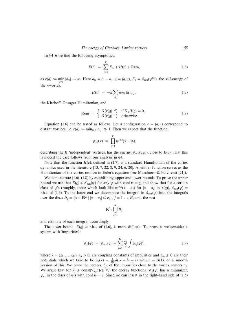
In § 4–6 we find the following asymptotics:

E(c) =

K∑i=1

Eni +H(c) + Rem, (1.6)

as r(a) := minij|aij | → ∞. Here aij = ai − aj , c = (a, n), En = Eren(ψ(n)), the self-energy of

the n-vortex,

H(c) = −π∑ij

ninj ln |aij |, (1.7)

the Kirchoff–Onsager Hamiltonian, and

Rem =

O(r(a)−2

)if ∇aH(c) = 0,

O(r(a)−1

)otherwise.

(1.8)

Equation (1.6) can be tested as follows. Let a configuration c = (a, n) correspond to

distant vortices, i.e. r(a) := minij |aij | 1. Then we expect that the function

ψ(0)(x) =

K∏i=1

ψ(ni)(x− ai),

describing the K ‘independent’ vortices, has the energy, Eren(ψ(0)), close to E(c). That this

is indeed the case follows from our analysis in § 4.

Note that the function H(c), defined in (1.7), is a standard Hamiltonian of the vortex

dynamics used in the literature [13, 7, 22, 8, 9, 24, 6, 20]. A similar function serves as the

Hamiltonian of the vortex motion in Euler’s equation (see Marchioro & Pulvirenti [21]).

We demonstrate (1.6)–(1.8) by establishing upper and lower bounds. To prove the upper

bound we use that E(c) 6 Eren(ψ) for any ψ with conf ψ = c, and show that for a certain

class of ψ’s (roughly, those which look like ψ(nj )(x − aj) for |x − aj | r(a)), Eren(ψ) =

r.h.s. of (1.6). To the latter end we decompose the integral in Eren(ψ) into the integrals

over the discs Dj = x ∈ R2 | |x− aj | 6 r0, j = 1, . . . , K , and the rest

R2\K⋃j=1

Dj

and estimate of each integral accordingly.

The lower bound, E(c) > r.h.s. of (1.6), is more difficult. To prove it we consider a

system with ‘impurities’:

Eλ(ψ) = Eren(ψ) +

K∑j=1

λj

2

∫δbj |ψ|2, (1.9)

where λ = (λ1, . . . , λK ), λj > 0, are coupling constants of impurities and δbj > 0 are their

potentials which we take to be δb(x) = 12πrδ(|x − b| − r) with r = O(1), or a smooth

version of this. We place the centres, bj , of the impurities close to the vortex centers aj .

We argue that for λj > const|∇ajE(c)| ∀j, the energy functional Eλ(ψ) has a minimizer,

ψλ, in the class of ψ’s with conf ψ = c. Since we can insert in the right-hand side of (1.5)


the condition |ψ| 6 1 without changing the result, we have

E(c) > Eλ(c)−K∑j=1

λj , (1.10)

where Eλ(c) = Eλ(ψλ).On the second step, using the Euler–Lagrange equation,

−∆ψ + (|ψ|2 − 1)ψ = −Σλjδbjψ, (1.11)

for ψλ, we show that ψλ belongs to the class of functions used in the proof of the upper

bound. Hence, Eλ(c) = Eλ(ψλ) is of the form of the right-hand side of (1.6). This completes

the proof of the lower bound and therefore of (1.6).

Equation (1.11) is rather subtle. We analyze it using an implicit function theorem.

Denote the map ψ → −∆ψ+(|ψ|2−1+

∑λjδbj

)ψ by G0(ψ). Let ψ0(x) be an approximate

solution to (1.11) (e.g. see the function ψ(0)(x) above). Expanding G0(ψ) around ψ0 we

rewrite (1.11) as

L0(ξ) = −G0(ψ0)−N(ξ), (1.12)

where ξ := ψ − ψ0, the operator L0 is the linearization of G0(ψ) around ψ0 and N(ξ)

is the nonlinear in ξ part of G0(ψ0 + ξ). The next step is to invert the operator L0, and

consider the resulting equation as a fixed point equation. However, here we run into a

problem. First, the continuous spectrum of the operator L0 fills the positive semiaxis [0,∞)

going all the way to 0. Secondly, L0 has near zero modes due to the fact that the vortex

solutions ψ(nj )(x − aj), j = 1, . . . , K , break the translational (as well as rotational/gauge)

symmetry of the original equation (1.1). These near zero modes have long-range tails, and

as a result, they interact rather strongly even at large distances. A careful analysis carried

out in § 6 stipulates convincingly that (1.11) has a solution of the desired form, provided

the strengths, λj , and locations, bj , of the impurities are adjusted in such a way that the

right-hand side of the resulting equation (1.12) is orthogonal to the corresponding (near)

zero translational modes. Thus, we remove small denominators and secular terms so that

the perturbation theory is valid.

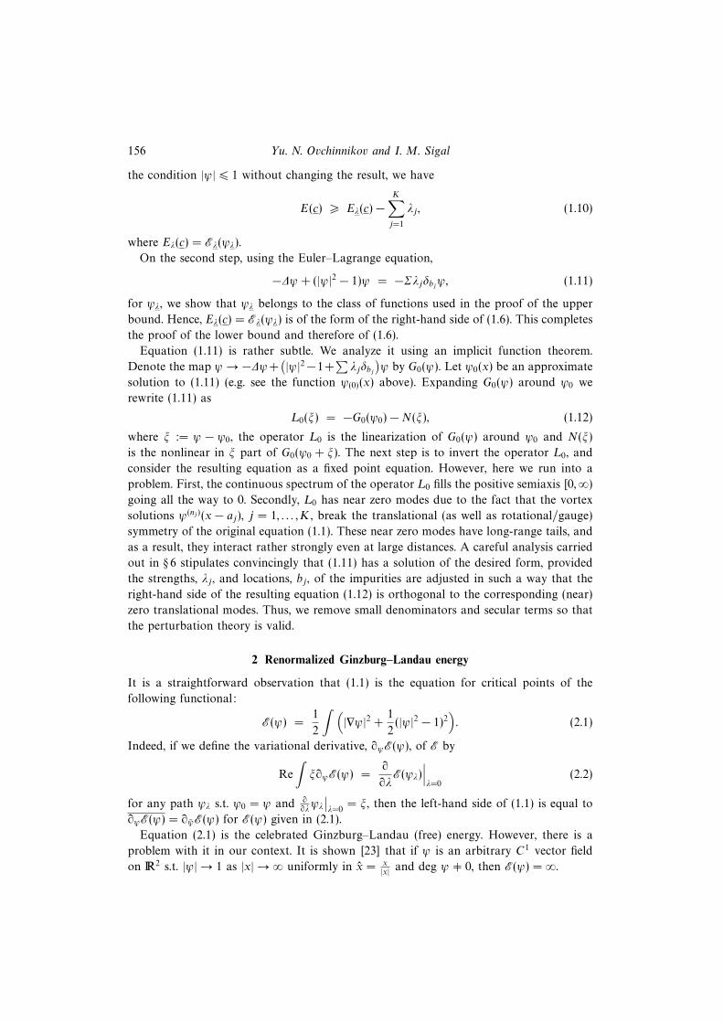
2 Renormalized Ginzburg–Landau energy

It is a straightforward observation that (1.1) is the equation for critical points of the

following functional:

E(ψ) =1

2

∫ (|∇ψ|2 +

1

2(|ψ|2 − 1)2

). (2.1)

Indeed, if we define the variational derivative, ∂ψE(ψ), of E by

Re

∫ξ∂ψE(ψ) =

∂

∂λE(ψλ)

∣∣∣λ=0

(2.2)

for any path ψλ s.t. ψ0 = ψ and ∂∂λψλ∣∣λ=0

= ξ, then the left-hand side of (1.1) is equal to

∂ψE(ψ) = ∂ψE(ψ) for E(ψ) given in (2.1).

Equation (2.1) is the celebrated Ginzburg–Landau (free) energy. However, there is a

problem with it in our context. It is shown [23] that if ψ is an arbitrary C1 vector field

on R2 s.t. |ψ| → 1 as |x| → ∞ uniformly in x = x|x| and deg ψ 0, then E(ψ) = ∞.


We renormalize the Ginzburg–Landau energy functional as follows (see Ovchinnikov

& Sigal [23]). Let χ(x) be a smooth real function on R2 s.t.

χ(x) =

1 for |x| > R + R−1,

0 for |x| 6 R.(2.3)

Define

Eren(ψ) =1

2

∫ (|∇ψ|2 − (deg ψ)2

r2χ+ F(|ψ|2)

)d2x (2.4)

where

F(u) =1

2(u− 1)2 . (2.5)

We list here the most important properties of Eren(ψ) (see Ovchinnikov & Sigal [23] for

the proofs):

(a) ∂ψEren(ψ) = −∆ψ + F ′(|ψ|2)ψ.

(b) Given n let Mn =ψ = feiϕ | ∫

|x|>2

1r2 |1 − f2| < ∞, f is continuous and f(0) = 0,∫ |∇(ϕ− nθ)|r−1 < ∞ and

∫ |∇(ϕ− nθ)|2 < ∞

. Then Eren(ψ) < ∞ ∀ψ ∈Mn.

(c) We have the following bound from below:

Eren(ψ) > EB(0,R)(ψ) +1

2

∫|x|>R

(∣∣∇|ψ|∣∣2 − 1

2|∇ϕ|4

)d2x, (2.6)

where R = R + R−1, ϕ = arg ψ, and for Ω ⊂ R2,

EΩ(ψ) =1

2

∫Ω

(|∇ψ|2 − (deg ψ)2

r2χ+ F(|ψ|2)

)d2x. (2.7)

3 The energy of vortex configurations

In this section we discuss the connection between −∇E(c), the force acting on the vortex

centers, and the existence of a minimizer for the variational problem (1.5). It is clear

intuitively that such a minimizer exists if and only if ∇E(a) = 0. However, to establish

this fact is not so easy. In what follows n is fixed and we use the notation E(a) = E(c)

and H(a) = H(c) for c = (a, n). We begin our analysis with

Proposition 3.1 If there is a minimizer for variational problem (1.5), then this minimizer

satisfies the Ginzburg–Landau equation (1.1).

Proof. Let ψ be a minimizer for (1.5). Since for any differentiable function ξ: R2 → Cvanishing together with its gradient sufficiently fast at ∞ and vanishing at the points

a1, . . . , am we have

0 =∂

∂λEren(ψ + λξ)

∣∣∣λ=0

= Re

∫ξ(− ∆ψ + (|ψ|2 − 1)ψ

),


we conclude that ψ satisfies (1.1) for x a1, . . . , am. On the other hand, since ψ ∈ H loc1 (R2),

we have that −∆ψ + (|ψ|2 − 1)ψ ∈ H loc−1 (R2). Hence −∆ψ + (|ψ|2 − 1)ψ = 0 on R2. q

We assume that the function E(a) is differentiable and that there are approximate

minimizers ψ(ε)a s.t. ∇Eren(ψ(ε)

a )→ ∇E(a) as ε→ 0, pointwise in a. Then we have

Theorem 3.2 Let ∇E(a) 0. Then the variational problem (1.5) has no minimizer.

Proof. Assume, on the contrary, that problem (1.5) has a minimizer, ψa. By Proposition

3.1 it solves (1.1) and therefore is a critical point of the functional Eren(ψ). Assume first

that there is a path a(t), 0 6 t 6 ε, for some ε > 0, in R2n, starting at a in the direction e

s.t. e · ∇E(a) 0 and problem (1.5) has minimizers, ψa(t), for the points a(t). Then

d

dtEren(ψa(t))

∣∣∣t=0

= a(0) · ∇E(a) 0,

which contradicts to the statement that ψa is a critical point of Eren(ψ). If (1.5) has no

minimizers for any curve a(t), 0 < t 6 ε, s.t. a(0) = a and a(0) · ∇E(a) 0, then we pick

approximate minimizers in accordance with the above condition and proceed as in the

argument above. q

We conjecture that the assumptions formulated above are always satisfied. (Approximate

minimizers which we expect satisfy it are constructed in § 5 by a method of impurities.) In

any case, the proof above shows that minimizers of (1.5) can be located only on a discrete

set of level sets of the function E(a).

4 Asymptotics of energy of vortex configurations. Upper bound

In this section we study asymptotics of the energy, E(a), of vortex configurations (a, n) as

r(a) → ∞. Recall that r(a) = minij|aij |. In what follows the parameter R in (2.3) is taken

to be sufficiently large, and we display the R-dependence in the energies by writing ER(a)

for E(a) and En,R for En. Our main result is the following relation:

ER(a) = E(0)R + Rem + O

(1

R2

), (4.1)

where

E(0)R =

∑i

Eni,R +H( aR

)(4.2)

and the remainder, Rem, satisfies the estimate

Rem =

O(r(a)−2

)if ∇H(a) = 0

O(r(a)−1

)otherwise

(4.3)

We demonstrate (4.1) by verifying that its right-hand side is an upper and lower bound

for the left-hand side. The upper bound is obtained in this section, while the lower one is

obtained in the next one.


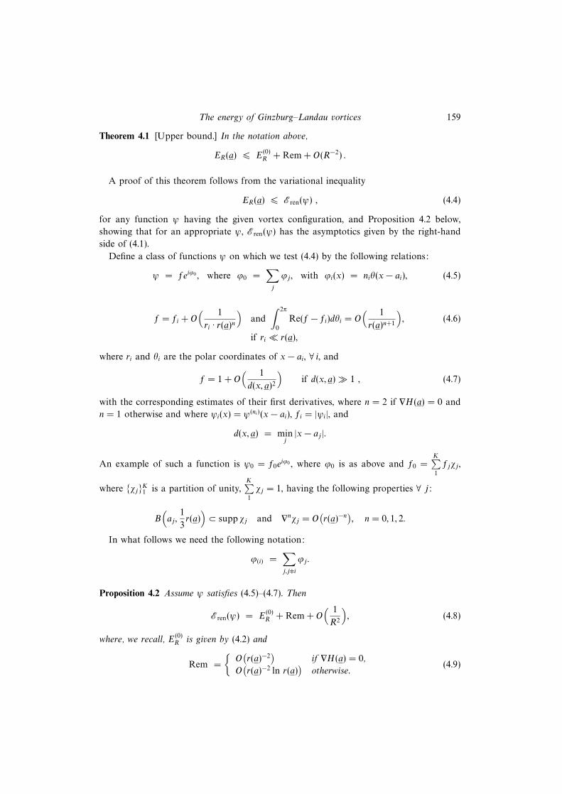
Theorem 4.1 [Upper bound.] In the notation above,

ER(a) 6 E(0)R + Rem + O(R−2) .

A proof of this theorem follows from the variational inequality

ER(a) 6 Eren(ψ) , (4.4)

for any function ψ having the given vortex configuration, and Proposition 4.2 below,

showing that for an appropriate ψ, Eren(ψ) has the asymptotics given by the right-hand

side of (4.1).

Define a class of functions ψ on which we test (4.4) by the following relations:

ψ = feiϕ0 , where ϕ0 =∑j

ϕj , with ϕi(x) = niθ(x− ai), (4.5)

f = fi + O( 1

ri · r(a)n)

and

∫ 2π

0

Re(f − fi)dθi = O( 1

r(a)n+1

), (4.6)

if ri r(a),

where ri and θi are the polar coordinates of x− ai, ∀ i, and

f = 1 + O( 1

d(x, a)2

)if d(x, a) 1 , (4.7)

with the corresponding estimates of their first derivatives, where n = 2 if ∇H(a) = 0 and

n = 1 otherwise and where ψi(x) = ψ(ni)(x− ai), fi = |ψi|, and

d(x, a) = minj|x− aj |.

An example of such a function is ψ0 = f0eiϕ0 , where ϕ0 is as above and f0 =

K∑1

fjχj ,

where χjK1 is a partition of unity,K∑1

χj = 1, having the following properties ∀ j:

B(aj ,

1

3r(a))⊂ supp χj and ∇nχj = O

(r(a)−n

), n = 0, 1, 2.

In what follows we need the following notation:

ϕ(i) =∑j,ji

ϕj .

Proposition 4.2 Assume ψ satisfies (4.5)–(4.7). Then

Eren(ψ) = E(0)R + Rem + O

( 1

R2

), (4.8)

where, we recall, E(0)R is given by (4.2) and

Rem =

O(r(a)−2

)if ∇H(a) = 0,

O(r(a)−2 ln r(a)

)otherwise.

(4.9)


Remark 4.1. Of course, to prove the upper bound in Theorem 4.1 it suffices to estimate

Eren(ψ) for one function only, so we can take, for example, f = fj for |x− aj | r(a) ∀ j.However, Proposition 4.2 is also used below (see § 5) to obtain a lower bound on ER(a).

Proof. Let Dj = D(aj , r0), the disc with the centre at aj and of the radius r0. We specify

r0 as r0 <12r(a) and r0 = O(r(a)). We decompose the energy functional as

Eren(ψ) =∑j

∫Dj

e(ψ) +

∫(∪Dj )c

e(ψ), (4.10)

where Dc := R2\D and e(ψ) is the energy density,

e(ψ) =1

2|∇ψ|2 +

1

4(|ψ|2 − 1)2.

Let e1(ϕ) = 12|∇ϕ|2 and 〈f(ψ)〉 = f(ψ)−∑

k

f(ψk). Eqn (4.7) implies∫(∪Dk)c

e(ψ) =

∫(∪Dk)c

e1(ϕ0) +

∫(∪Dk)c

O(d(x, a)−4

). (4.11)

Next, the estimates

|ψi| = 1 + O(r−2i ) (4.12)

and

∇|ψi| = O(r−3i ) (4.13)

give ∫(∪Dk)c

e1(ϕi) =

∫(∪Dk)

e(ψi) + O(r−20 ). (4.14)

This together with (4.11) yields∫(∪Dk)c

〈e(ψ)〉 =1

2

∑ij

∫(∪Dk)c

∇ϕi∇ϕj + O(r−20 ). (4.15)

Next, we write ψ in the region Di as ψ = eiϕ0 (fi + ξ), where fi ≡ |ψi|. As a single-valued

harmonic function in Di, ϕ(i) has the following expansion

ϕ(i) =

∞∑m=0

cmrmi cosm(θi − β(m)

i ),

where, we recall, ri and θi are the polar coordinates of x − ai and cm and β(m)i are some

constants. This implies that ∫Di

∇ϕi · ∇ϕ(i) = 0.

Using this relation and that∫Dj

fj∇ϕj · ∇ Im ξ = nj

∫Dj

fj∂

∂θIm ξ = 0,

we obtain ∫Di

e(ψ) =

∫Di

e(ψi) +

∫Di

e1(ϕ(i)) + R1 + R2,


where

R1 =

∫Di

(f2i − 1)

(∇ϕi · ∇ϕ(i) +

1

2|∇ϕ(i)|2

),

and

R2 =

∫Di

(|∇ϕ0|2 + f2

i − 1)fiRe ξ + f2i (Re ξ)2

+1

2|∇ϕ0|2|ξ|2 +

1

2|∇ξ|2 + 2∇fi · ∇Re ξ + fi∇ϕ(i) · ∇Im ξ

+Im(ξ∇ϕ0 · ∇ξ) +1

2(f2i − 1 + 2fiRe ξ)|ξ|2 +

1

4|ξ|4.

Using that |∇ϕ(i)(x)|2 = O(d(x, a)−2

)and ∇ϕi(x) = O(r−1

i ), expanding

∇ϕ(i)(x) = ∇ϕ(i)(ai) + O( ri

r(a)2

)and using that

∫Di

(1− f2i )∇ϕi = 0, we obtain

R1 = O( ln r0r(a)2

).

Using that, due to (4.6), ξ = O(

1r·r(a)

)and

∫ 2π

0 Re ξ dθ = O(

1r(a)2

), and using that

|∇ϕi|2 + f2i − 1 = O(r−4

i ), we find

R2 = O( ln r0r(a)2

).

Finally, we observe that due to (4.14),

1

2

∫Dk

|∇ϕ(k)|2 =∑jk

∫Dk

(e1(ψj) + I

)=∑jk

∫(e(ψj) + I) + O(r−2

0 ),

where I := 12

∑ij ∇ϕi∇ϕj . Collecting the estimates above, we arrive at∫

Dk

(〈e(ψ)〉 − I) = O( ln r0r(a)2

)+ O

( 1

r20

), (4.16)

which together with (4.10) and (4.15) yields

Eren(ψ) = E + O( 1

r20

), (4.17)

where E =∫ (

g − n2

r2 χ)

with g =∑j

e(ψj) + I and n = deg ψ.

Now, by the definition of the cut-off function χ (χ > 0, χ = 1 for |x| > R) we have

E 6

∫DR

g +

∫DcR

(g − n2

2r2

), (4.18)

where DR is the disc around the origin of radius R. Now, by the definition (ai R)∫DR

e(ψi) =

∫DR+ai

e(ψ(ni)) = Eni,R + O( 1

R2

). (4.19)


Next, we show that

1

2

∫DR

∇ϕi∇ϕj = −πninj ln( |aij |R

). (4.20)

We compute ∫DR

∇ϕi∇ϕj = ninj

∫ 2π

0

∫ R

0

r − a cos θ

r2 + a2 − 2ar cos θdr dθ,

where a = |aij |. Furthermore,∫ 2π

0

r − a cos θ

r2 + a2 − 2ar cos θdθ =

2π

r

1 if r > a,

0 if r < a.

The last two equations yield (4.20). Observe also that up to a multiplicative constant

expression (4.20) can be found from symmetry considerations: the invariance of the

integral on the left-hand side under translations (ai → ai + h and aj → aj + h ∀h ∈ R2)

and rotations (ai → gai and aj → gaj ∀g ∈ O(2)) imply that it depends only upon |aij |.Its scaling properties under the dilations (ai → λai and aj → λaj ∀λ ∈ R) imply that it is

a multiple of ln( |aij |

R

).

Equations (4.19) and (4.20) imply∫DR

g =∑

Eni,R +H(a/R) + O(1/R2). (4.21)

Next we estimate the second integral on the r.h.s. of (4.18). By Eqns (4.13) and (4.14)

we have

g =1

2|∇ϕ0|2 + O

(d(x, a)−4

).

Furthermore, expanding the terms ∇θ(x − aj) in ∇ϕ0(x) =∑nj∇θ(x − aj) around the

point x we obtain

∇ϕ0(x) = n∇θ(x)− θ′′(x)∑

njaj + O(∑ nja

2j

d(x, a)3

), (4.22)

where θ′′(x) is the Hessian of θ(x). Choosing the origin so that∑njaj = 0 eliminates the

second term on the right-hand side. (Otherwise we could have used that by an explicit

computation we have

θ′′(x)∇θ(x) = − x

r4,

the integral of which over the exterior of the ball B(0, R) vanishes.) Hence∫DcR

(g − n2

2r2

)=

∫DcR

O(∑ nja

2j

d(x, a)4

)(4.23)

= O(∑ nja

2j

R2

). (4.24)

Equations (4.17)–(4.21) with r0 = O(r(a))

and Eqn (4.23) imply (4.8) with Rem =

O(

ln r(a)r(a)2

). Similarly, one obtains (4.8)–(4.9) in the forceless case. q


Remark 4.2. The estimate (4.9) can be considerably improved in the force-free case, if we

use instead of e1(ϕ) = 12|∇ϕ|2 the density

e2(ϕ) =1

2|∇ϕ|2 − 1

2|∇ϕ|4,

which is a better approximation to the density e(ψ), and instead of (4.12) and (4.13) we

use

|ψi| = 1− 1

2|∇ϕi|2 + O(r−4

i ) (4.25)

and

∇|ψi| = −1

2∇|∇ϕi|2 + O(r−5

i ), (4.26)

respectively. Indeed, proceeding as above, we find in the force-free case that

E(ψ) = E(0)R +K + O

(ln r(a)

r(a)4

)+ O

(1

R2

), (4.27)

where

K = −1

2

∫DR

|∇ϕ0|4 −∑j

|∇ϕj |4 . (4.28)

This result is used in Ovchinnikov & Sigal [26].

5 Lower bound on energy of vortex configurations. Pinning effect

Lower bounds are notoriously difficult. An additional problem which faces us is that

unless the condition ∇ER(a) = 0 is satisfied minimization problem (1.5) has no minimizer.

To circumvent the latter difficulty we introduce defects into the system, and use the fact

that sufficiently strong defects bind the vortices (the effect of pinning). More precisely, we

introduce the new energy functional

Eλ(ψ) = ER(ψ) + Σ1

2λj

∫δbj |ψ|2, (5.1)

where λ = (λ1, . . . , λK ), λj > 0, are coupling constants of the defects and δbj > 0 are their

potentials, centered at points bj ∈ R2 depending on a and very close to the aj ’s. The λj ’s

and bj ’s will be determined later. We take δb to be either

δb =1

2πrδ(|x− b| − r), (5.2)

where r = O(1), or a smooth version of this, i.e. δb is a smooth function supported in the

annulus

x ∈ R2 | r 6 |x− b| 6 r + δ (5.3)

for some sufficiently small δ and satisfying∫δb = 1. (5.4)

Remark 5.1. Sometimes it is convenient to modify the definition of δb in such a way

that ∀j, δbj fj does not contain harmonics in θ with |m| > 2, where (r, θ) are the polar


coordinates of y = x− aj (see the harmonic analysis of (6.8) in the next section). To this

end, we replace (5.2) by

δb =1

2πr

∂γ

∂r(x− b)δ(γ(x− b)),

where γ(x) is a slight deformation (modulation) of the function |x| − r, or by a smooth

version of the latter function, so that∫ 2π

0

δbj fjeimθdθ = 0 for |m| > 2.

With the potential δb defined as above it is argued below that Eλ(ψ) has a minimizer

among functions with the given vortex configuration (a, n), provided

λj > C|∇ajE(a)| (5.5)

for an appropriate constant C .

We argue as follows. Clearly, a minimizer, if it exists, has near aj the form of the jth

vortex, ψj, ∀j . The relevant contribution of the second term on the right-hand side of (5.1)

near aj is 12λj∫δbj |ψ|2. If the centre of the vortex is at the centre of the ring supp δbj , i.e.

aj = bj , then the contribution of this term is approximately 12λjα

2njε2nj , where ε = r is the

radius of the interior boundary of the support of δbj , provided ε 1 and αnj is defined

by the expansion

|ψ(n)(x)| = αn|x|n + O(|x|n+2) (5.6)

for |x| 1 (remember, ψj(x) = ψ(nj )(x−aj)). On the other hand, if the centre of the vortex

is in supp δbj (i.e. aj ∈ supp δbj ), then the corresponding contribution is approximately

1

2λj

∫δbj f

2j =

1

2λjα

2nj

ε2nj

2π

∫ 2π

0

(2 cos

θ

2

)2njdθ

=1

2λjα

2njε2nj(

2njnj

).

Since(

2njnj

)> 1, this shows that it is more energetically advantageous for the vortex to be

inside the ring, supp δbj , than in its middle. Moreover, the force needed to remove the

vortex from the inside of the ring is approximately

1

2λj

∫δbj

∂

∂rfj = −2

πλjnjα

2njε2nj−1

2nj−1∑m=0

(−1)nj−m(

2nj−1m

)2(nj − m)− 1

, (5.7)

where we have used that∫ π

0

(2 cos

θ

2

)2nj−1

dθ = −2

2nj−1∑m=0

(−1)nj−m(

2nj−1m

)2(nj − m)− 1

.

On the other hand, the force with which the remaining vortices act on the jth vortex is

−∇ajE(a). This shows that for a fixed ε, to keep the j-th vortex inside the ring supp δaj we

need λj = O(|∇ajE(a)|), hence condition (5.5) for the existence of minimizer for energy

functional (5.1).


Remark 5.2. In fact, the force −∇aj · 12λj∫δbj f

2j ≈ 1

2λj · ∇f2

j (|bi− aj |) exerted on the vortex

j by the defects is also present when the vortex is outside of the defect ring and it takes

its greatest value at the distance r0 defined by

∂2f2j

∂r2

∣∣∣r=r0

, = 0, (5.8)

provided ε = r 1. This greatest value is

Fmax = λj∂f2

j

∂r

∣∣∣r=r0

. (5.9)

This implies, in particular, that the range of the potential created by the defect is O(1).

The minimizer, ψλ, of Eλ(ψ) satisfies the Euler-Lagrange equation

−∆ψ + (|ψ|2 − 1)ψ = −Σλjδbjψ. (5.10)

An analysis of this equation conducted in the next section shows that this minimizer

satisfies conditions (4.5)–(4.7). Then Proposition 4.2 implies that the energy

Eλ(a) := infEλ(ψ) | conf ψ = c (5.11)

which is equal to Eλ(ψλ), satisfies

Eλ(a) = E(0)R +

∑ 1

2λj

∫δbj |ψλ|2 + Rem + O

( 1

R2

), (5.12)

where Rem is given in (5.9). On the other hand, since the infimum can be taken over ψ’s

with |ψ| 6 1, we have that

ER(a) > Eλ(a)− Σλj. (5.13)

Due to (5.5), Σλj can be taken to be of the same order as Rem. Hence, we conclude that

ER(a) > E(0)R + Rem + O

( 1

R2

)(5.14)

with Rem given in (4.3).

6 Equation (5.10): method of geometric solvability

In this section we show that (5.10) has a solution satisfying (4.5)–(4.7), provided condition

(5.5) (or (6.11)) holds. This solution is the minimizer of variational problem (5.11). This

result was used in § 5 to obtain estimate (5.12).

We explain the main ideas of our method. We rewrite (5.10) as G(f) = 0, where

f = e−iϕ0ψ, and the map G is defined by

G(f) : = e−iϕ0(− ∇(eiϕ0f) + (|eiϕ0f|2 − 1 +

∑λjδbj )e

iϕ0f)

= −∆∇ϕ0f + (f2 − 1 +

∑λjδbj )f,

with ∆A := ∇2A, ∇A := ∇ + iA. Let ψ0 = f0e

iϕ0 be an approximate solution to (5.10), i.e.

f0 is an approximate solution to G(f) = 0. We look for a solution of the latter equation

in the form

f = f0 + ξ (6.1)


where ξ is a small fluctuation of the order O( 1r(a)

). We expand

G(f0 + ξ) = G(f0) + L(ξ)− R(ξ),

where L is the linearized operator for the map f → G(f) around the function f0:

L(ξ) := [−∆∇ϕ0+ f2

0 − 1 +∑

λjδbj ]ξ + 2f0Re(f0ξ)

and the term R(ξ) is the nonlinear in ξ part of G(f0 + ξ):

R(ξ) = −2ξRe(f0ξ)− |ξ|2ξ.Note that the operator L is self-adjoint in the inner product 〈ξ, y〉 := Re

∫ξy. Now the

equation G(f0 + ξ) = 0 can be rewritten as

L(ξ) = −G(f0) + R(ξ). (6.2)

The first task now is to show that this equation can be solved for ξ. We demonstrate

this nonrigorously by showing that for the choice of the parameters as mentioned above,

the right-hand side – in the leading order – is orthogonal to the almost zero modes of

the adjoint operator L∗ (= L). The latter modes are just the zero modes of the operator

e−iϕj · Lψj · eiϕj =: Lj , where Lψj are the linearizations of the original equation (1.1), i.e.

of the map ψ → ∆ψ + (|ψ|2 − 1)ψ, around the shifted vortex solutions ψj . They are due

to the fact that the vortex solutions, ψj , brake the translational (and rotatonal/gauge)

symmetry of the original equation (1.1).

Finally, we specify the approximate solution, f0, mentioned above. We define f0 so that

f0 = fj in Dj , 1 6 j 6 k , and f0 = 1 + O

(1

r(a)2

)in D0,

with the corresponding estimates on the derivatives of the remainder in the last equation.

Such a function can be constructed with the help of an appropriate partition of unity (see

the paragraph after equation (4.7) and the end of this section).

Now we proceed to the analysis of (6.2). We study (6.2) in each of the domains

Dj = x ∈ R2 | |x − aj | 6 r0, j = 1, . . . , K , and D0 = x ∈ R2 | |x − aj | > r1∀j, where

r0 r(a) and r1 1, separately.

The disc Dj , 1 6 j 6 k

We fix j and set r = rj . In Dj we have

L = Lj + O(1

r(a))

where the operator Lj was defined above and can be explicitly written out as

Lj(ξ) = (−∆+ |∇ϕj |2 + 2f2j − 1)ξ − 2i∇ϕj · ∇ξ + f2

j ξ,

and

−G(f0) = Fj + |∇ϕ(j)|2fj ,where

Fj = λjδbj fj + 2i∇ϕ(j) · (∇fj + i∇ϕjfj). (6.3)


Here we used that |∇ϕ0|2 − |∇ϕj |2 = 2∇ϕ(j) · ∇ϕj + |∇ϕ(j)|2. Observe that

eiϕj (∇fj + i∇ϕjfj) = ∇ψ;

is the translational zero mode of the operator Lψj and ∇fj + i∇ϕjfj is the zero mode of

the operator Lj .

Thus, the equation (6.2) can be written as

Lj(ξ) = Fj + Rj(ξ), (6.4)

where Fj is the leading part of a free term defined in (6.3) and Rj(ξ) = F ′ +R′(ξ) +R′′(ξ)

with

F ′ = −|∇ϕ(j)|2fj , (6.5)

R′(ξ) = −λjδbj ξ − (|∇ϕ0|2 − |∇ϕj |2)ξ + 2i∇ϕ(j) · ∇ξ, (6.6)

and

R′′(ξ) = −fj |ξ|2 − 2fj(Re ξ)ξ − |ξ|2ξ. (6.7)

Observe that the term∑ijλiδbiψ is absent, since it is zero in the region |x− aj | r(a).

Assuming ξ = O(

1r(a)

)and dropping the term Rj(ξ), which is of the order O

(1

r(a)2

), from

the right-hand side of (6.7), we arrive at the equation

Lj(ξ) = Fj. (6.8)

As mentioned above, the operator Lj is related to the operator Lψj , obtained by linearizing

(1.1) around the solution ψj (see Ovchinnikov & Sigal [23]), as follows:

Lj(ξ) = e−iϕjLψj (eiϕj ξ). (6.9)

Observe that Lj is self-adjoint, L∗j = Lj , in the scalar product

〈η, ξ〉 = Re

∫ηξ.

The only zero modes of the operator L∗j = Lj , which decay at ∞, are those related to the

translation symmetry of the equation, namely

ηk = e−iϕj∂xkψj , k = 1, 2. (6.10)

Hence, (6.8) is solvable only if

Re

∫ηkFj = 0 for k = 1, 2. (6.11)

Below we will find conditions on λj and bj for (6.11) to hold. For the moment we assume

(6.11) and push on with our analysis.

Expand ξ in (6.8) in the Fourier series

ξ(x) =

∞∑m=−∞

ξ(m)(r)eimθ, (6.12)

and define

ξ =⊕m>0

(ξ(m)

ξ(−m)

). (6.13)


Then, obviously ξ and ξ are in one-to-one correspondence, which we denote by ξ ↔ ξ.

Observe now that if ξ ↔ ξ, then

Ljξ ↔ Lξ :=⊕m>0

L(m)

(ξ(m)

ξ(−m)

), (6.14)

where

L(m) =

(−∆r +

(nj+m)2

r2 + 2f2j − 1 f2

j

f2j −∆r +

(nj−m)2

r2 + 2f2j − 1

).

Here ∆r stands for the radial Laplacian, ∆rf = r−1∂r(r∂rf) and we have used that

ϕj(x) = njθ(x− aj). Eqn (6.14) implies that (6.8) can be rewritten as

Lξ = F , (6.15)

where F =⊕m>0

(F (m)

F (−m)

)with

F (m)(r) = (2π)−1

∫ 2π

0

Fje−imθdθ. (6.16)

Finally, observe that the translational zero modes (6.10) in the new representation become

η1 = iη2 =⊕m>0

1

2

(f′j − nj

rjfj

f′j +njrjfj

)δm,1. (6.17)

This formula implies that (6.11) is equivalent to the relation∫ ∞0

(f′j − nj

rjfj

f′j +njrjfj

)·(F (1)

F (−1)

)rdr = 0. (6.18)

We analyze the operators L(m), m > 0. The operator-matrix L(0) can easily be diag-

onalized. A Perron–Frobenius argument given in Ovchinnikov & Sigal [23] shows that

L(0) > 0 and 0 is not an eigenvalue of L(0). Next, a similar (but more subtle) argument

shows that L(1) > 0 and 0 is a non-degenerate eigenvalue of L(1) (with the eigenfunction(f′j − nj

rjfj , f

′j +

njrjfj

)corresponding to the breaking of the translational symmetry of the

Ginzburg–Landau equation by ψj (see Ovchinnikov & Sigal [23] for details). Here f′jstands for the derivative of fj w.r. to rj = |x− aj |. Finally,

L(m) − L(1) =m− 1

r2j

(2nj + m+ 1 0

0 −2nj + m+ 1

)> 0

and) 0 for m > 2nj−1. Hence L(m) > 0 and 0 is not an eigenvalue of L(m) for m > 2nj−1.

For 2 6 m < 2nj − 1, L(m) have negative eigenvalues, but still do not have an eigenvalue

at zero (note that in general such eigenvalues, unless related to symmetries, are unstable

and can be easily removed by small perturbations). We leave this fact without a proof

since we can choose δbj so that F (m) = 0 for |m| > 2 (see Remark 5.1), so that we can

solve (6.22) without using properties of the operators L(m), m > 2.


Due to condition (6.11), (6.18) has a unique solution which we write in the form

ξ = (L)−1F

=⊕m>0

G(m)

(F (m)

F (−m)

), (6.19)

where G(m) is the (left, if m = 1) inverse of L(m). Observe now that L(m) are (matrix)

ordinary differential operators, their (regularized) Green’s functions can be found in terms

of some special solutions to the homogeneous equations. This is done in Ovchinnikov &

Sigal [27]. (It is convenient for technical reasons to include a part of R′(ξ) into Lj(ξ),

namely, to replace Lj in (6.8) by Lj + λjδbj .) Results of [27] imply that ξ is of the

same order as F , i.e. as will be shown below, O(

1r(a)2

)in the forceless case and O

(1r(a)

),

otherwise. This, due to (6.1) and (6.12), implies (4.5) and the first part of (4.6).

Region D0

In this region (5.10) coincides with Ginzburg–Landau equation (1.1), i.e. the right-hand

side of (5.10) vanishes. In this region

L = L0 + O(1

r(a)2),

where the operator L0 is related to the linearization of the map ψ → ∆ψ + (|ψ|2 − 1)ψ

around eiϕ0 ,

L0(ξ) :=(− ∆− 2i∇ϕ0 · ∇+ |∇ϕ0|2)ξ + 2Reξ, (6.20)

and

G(f0) = G(1) = |∇ϕ0|2 =: −F0.

Assuming that ∇nξ = O(r(a)−n−2

)in the region D0 and dropping terms of the order

O(r(a)−5

)we arrive at the equation

L0(ξ) = F0. (6.21)

Taking the real and imaginary parts of this equation, we obtain (to leading order in 1|x| )

Re ξ0 = −1

2|∇ϕ0|2 (6.22)

and

−∆Im ξ0 = −∇ϕ0 · ∇|∇ϕ0|2. (6.23)

The last two equations show that

|ξ0| = O( 1

d(x, a)2

)so that property (4.7) holds for the solution ψ. Moreover, these equations imply that ψ is

of the form

ψ = ei(ϕ0+Im ξ0)(

1− 1

2|∇ϕ0|2 + O

( 1

d(x, a)4

)), (6.24)

where we remember Im ξ0 solves (6.23).


To solve (6.23) we have to take into account the boundary conditions on ∂D0. Instead

of this, we use the solutions of (6.8) as sources. Namely, we proceed as follows. Writing

ϕ = ϕ0 + Im ξ

and using that λj are real, we derive from (5.10)

−∆Im ξ = ∇(ϕ0 + Im ξ) · ∇ ln f2, (6.25)

where, we recall, f = |ψ|. Observe that while ϕ0 is a multivalued function, Im ξ is a regular

function on R2 vanishing at ∞. Thus, (6.25) can be written as

Im ξ(x) =1

2π

∫ln |x− y|∇(ϕ0(y) + Im ξ(y)

) · ∇ ln f2(y)dy. (6.26)

Let ξj be the solution of equation (6.8) for j = 1, . . . , K , and of equations (6.22)–(6.23) for

j = 0, let fj = |ψj | for j = 1, . . . , K , and = 1 − 12|∇ϕ0|2 for j = 0. In the right-hand side

of (6.26) we take ξ = ξj in Dj , j = 0, . . . , K , where D0 = R2\⋃j

Dj . Plugging this into the

right-hand side of (6.26), we obtain the following equation for Im ξ0:

Im ξ0 =1

2π

K∑j=0

∫Dj

ln |x− y|∇ϕ0(y) · ∇ ln

(fj(y) + Re ξj

)2

+∇Im ξj(y) · ∇ ln fj(y)2d2y, (6.27)

where Im ξj , j = 1, . . . , k, are given as above. We iterate this equation. On the first step,

we drop Im ξ0 from the right-hand side. The resulting expression for Im ξ0 suffices for us.

The free term Fj (see (6.3))

In the rest of this section, we keep j fixed and let y = x − aj , and let r and θ be the

polar coordinates of the vector y. We consider the cases ∇ajH(a) 0 and ∇ajH(a) = 0

separately.

(a) ∇ajH(a) 0. The definition of H(a), (1.7) (recall that H(a) = H(c)), implies that

J∇ajH(a) = −2πnj∇ϕ(j)(aj), (6.28)

where, we recall, J =

(0 −1

1 0

). Using this equation and the fact that J∗ = −J , we

obtain that, modulo O(

1r(a)2

),

−2ie−iϕj∇ψj · ∇ϕ(j)

= − 1

πnjr

(if′jJy +

1

rfj y)· ∇ajH(a). (6.29)

Then, taking into account Remark 5.1, we obtain for the Fourier coefficients, F (m), of

Fj (see (6.16)) that

F (±m) = F (±1)δm,±1. (6.30)

Let kj = |kj |e−iαj be the complex number corresponding to the vector − 12πnj

J∇ajH(a).


We compute

F (±1) = i|kj |e∓iαj(f′j ∓ nj

rfj

)− 1

2π

∫ 2π

0

λjδbj fje∓iθdθ (6.31)

(a) ∇ajH(a) = 0. First, we observe that since ϕ(j) =∑

kj ϕk is a single-valued function

in the region r = |x−aj | < r(a) and is harmonic in R2, it has in this region the following

Fourier series expansion:

ϕ(j) =

∞∑m=0

cmrm cos m(θ − β(m)

j ) (6.32)

for some amplitudes cm and phases β(m)j (with cm = O

(r(a)−m

)). Moreover, in the force-

free configuration c1 = 0. Using this we find that in the force-free case, the expression

for (6.16) is

F (±m) = ±2iαre∓2iβ(2)j

(± f′j − nj

rfj

)δm,2 − 1

2π

∫ 2π

0

λjδbj fje∓iθδm,1, (6.33)

where the coefficient α is O(r(a)−2

)(see (6.32)).

Conditions on λj and bj

Now we derive the restrictions on the parameters λj and bj implied by solvability

conditions (6.11) or (6.18). We consider separately two cases.

(a) ∇ajH(a) 0. Let ~η =(η1

η2

), where ηj are given in (6.10). It is shown in Appendix A

that

Re

∫~ηFj = ∇ajH(a)− 1

2λj

∫δbj∇f2

j , (6.34)

where ∆aj = bj − aj . Equations (6.11) and (6.28) imply then that

1

2λj

∫δbj∇f2

j = ∇ajH(a). (6.35)

This fixes the direction in which the jth vortex centre, aj , must be shifted relative to

the center, bj , of the circle supp δaj . Indeed, it is shown in Appendix A that∫δbj∇f2

j ≈ 1

2∆ajf

2′j (r1).

This equation together with (6.21) implies that

λj = |∇ajH(a)|/|∆aj |f2′j (r1) if ∇ajH(a) 0 (6.36)

and that the direction ∆aj = ∆aj/|∆aj | should satisfy

∆aj = ∇ajH(a)/|∇ajH(a)| if ∇ajH(a) 0. (6.37)

(b) ∇ajH(a) = 0. Recall that the operator L(2) does not have a bounded zero mode.

Hence, due to (6.33), we can set λj = 0 when solving (6.15) to the order of O(r(a)−2

).

Hence, (6.15) has a unique solution O(r(a)−2

). The need for λj arises only in the next

step of the perturbation theory in the small term R(ξ), neglected previously, i.e. at

O(r(a)−3

). Thus, in this case we can take λj = O

(r(a)−3

)and so on.


Iteration scheme

Now we derive an equation allowing us to go beyond the first order perturbation theory.

To this end, we use the method of geometric parametrices of Sigal [30]. Let χjK0 be

the partition of unity, i.e.K∑j=0

χj = 1, s.t. supp χj ⊂ Dj . Let Gj be the left inverse (or the

(regularized) Green’s function) for the operator Mj = Lj − 2i∇ϕ(j) · ∇+ λjδbj , j = 0, . . . , K

(for j = 0 the last two terms on the right-hand side are absent). Assume the unknown

function ξ is orthogonal to the translational zero modes of the operators L1, . . . , LK .

Applying the operatorK∑j=0

χjGj to (5.10), and using (6.4) and the equations GjMj(ξ) = ξ

for j = 0, . . . , K , we obtain

ξ =

K∑j=0

χjGjFj +

K∑j=0

χjGjRj(ξ), (6.38)

where Rj(ξ) = Rj(ξ) − 2i∇ϕ(j) · ∇ξ + λjδbj ξ, and where we used that Mjξ = Fj + Rj(ξ).

Equation (6.38) is a fixed point problem. One can try to show that this problem has a

solution in an appropriate Banach space. This goal is outside the scope of this paper.

Here this equation is used to find the function ξ iteratively to an arbitrary order in 1r(a)

.

After that one recovers the solution ψ of (5.10) as

ψ = eiϕ0 (f0 + ξ). (6.39)

This analysis shows that in the leading order in perturbation theory (5.10) has a solution

satisfying (4.5)–(4.7) with n = 1, provided the λj ’s and bj ’s are s.t. (6.11) holds.

7 Conclusion

In this paper, we have introduced and analyzed the intervortex energy for the Ginzburg–

Landau equation. We have described its key role in finding (non-minimizing) multivortex

solutions, i.e. solutions ‘composed’ of several single vertices (in a separate paper [24] we

use the intervortex energy to describe dynamics of vortices). We also found its asymptotic

behaviour as the intervortex distances increase. A part of the latter result (upper bound –

easy part) is rigorous, while the other part (lower bound – hard part) is justified by detailed

analysis. This analysis uses an auxiliary energy functional – pinning energy functional –

which differs from the original one by extra potentials. The role of these potentials is to

hold down the vortices from moving as a result of mutual interactions. The infimum of

the pinning functional yields a lower bound on the original Ginzburg–Landau functional.

It is argued that the new functional has a local minimizer (the point important in its own

right as it relates to an important phenomenon of pinning) corresponding to the vortex

configuration of interest. (We venture that there should be a mountain pass-type argument

showing this.) Using the corresponding Euler–Lagrange (or modified Ginzburg–Landau)

equation we estimate this local minimizer and its energy. The latter energy gives a desired

lower bound on the Ginzburg–Landau energy under consideration.


Appendix A

In this appendix we perform some computations required in § 6. In what follows we set

r = |x− ai|.First prove (6.34). We claim that

Re

∫~η(Fj + λjδbj fj) = ∇ajH(a). (A 1)

Indeed, (6.17) shows that ηk , k = 1, 2, have only the m = ±1 harmonics. Using this

equation together with (6.3), or (6.34), we obtain

Re

∫~η(Fj + λjδbj fj) = −Re πikj

∫ ∞0

η · Jηrdr(

1

−i), (A 2)

where η =(f′j− nj

rfj

f′j+njrfj

). The right-hand side can be computed explicitly:

R.H.S. (A 2) = −Re πkj

∫ ∞0

(− 4

nj

rfjf

′j

)rdr

(i

1

)= 2πnjRekj

(i

1

).

Since kj is the complex version of − 12πnj

J∇ajH(a), (A 1) follows.

Now we compute the term Re∫ξkλjδbj fj under the assumption that |∆aj | r, where,

recall, ∆aj = bj − aj . To simplify the computations we let δbj be the true δ-function,

not a smeared one. Under the first assumption, the equation |x − bj | = r for the circle

(= supp δbj ) can be written in the leading approximation in ∆aj as

r ≈ r + ∆aj · y, (A 3)

where, remember, r and θ are the polar coordinates of y = x−aj . Thus, δbj = δ(|x−bj |− r)can be replaced by δ(r − r − ∆aj · y). This yields

Re

∫~ηδbj fj ≈

∫fjf

′j yδ(r − r − ∆aj · y)

≈ fj(r)f′j(r)2π∫

0

y(r + ∆aj · y)dθ.

Hence

Re

∫~ηδbj fj ≈ πfj(r)f

′j(r)∆aj. (A 4)

Appendix B Region Dj ∩ D0

Now we investigate the behaviour of the solution ξ in the regions Dj ∩ D0. We require

that asymptotics in Dj ∩ D0 of the solutions found in Dj and D0 match. We fix j and let

r and θ denote the polar coordinates of y = x− aj . As before we consider two cases.

∇ajH(a) 0

Now we find the leading asymptotic of ξ in the region 1 r r(a). Since only the


operator L(1) has a zero mode, the leading term for r 1 comes from the m = 1 sector.

Thus, we consider (6.15) in this sector:

L(1)

(ξ(1)

ξ(−1)

)=

(F (1)

F (−1)

). (B 1)

We write the solution of this equation in the form(ξ(1)

ξ(−1)

)=

(ξ

(1)0

ξ(−1)0

)+ c

(f′j − nj

rfj

f′j +njrfj

), (B 2)

where( ξ(1)

0

ξ(−1)0

)is a special solution, c is a constant and the vector which multiplies c is, recall,

the translational zero mode. The value of c is fixed from original nonlinear equation (6.4)

(say, by the perturbation theory). We show [27] that ξ(±1)0 are bounded.

Dropping in (B 1) the derivatives of ξ which are of a higher order in r−1 as well as the

terms f2j − 1 and

(nj±1)2

r2 in L(1), and dropping the terms coming from λjδbj and the terms

containing f′j from F(1)0 and F (−1)

0 , we arrive at the asymptotic equation(1 1

1 1

)(ξ(1)

ξ(−1)

)= −ikj nj

r

(1

1

). (B 3)

A particular solution of this equation,njkj2ir

(11

), and the asymptotics,

njr

(−11

), of the transla-

tional zero mode for r 1 lead to the asymptotics of the general solution to (6.15):(ξ(1)

ξ(−1)

)=

njkj

2ir

(1

1

)+ iνe−iαj

(−1

1

)(B 4)

plus higher order terms in r−1 (remember, kj = |kj |e−iαj ). Here ν is a function of r

(incorporating cnjr

); it cannot be found from (B 3) and an explicit expression for it will be

given below. This together with (6.12) yields the asymptotic expression for the solution to

(6.8):

ξj =nj |kj |r

sin(θ − αj)− 2iν · cos(θ − αj) (B 5)

plus higher order terms in r−1. The second term on the right-hand side yields, in the

leading order, a correction to the phase of ψ (due to a small translation of the center of

the vortex), while the first term, to |ψ|:ϕ = ϕj + 2ν cos(θ − αj) (B 6)

and

|ψ| = 1− n2j

2r2+nj |kj |r

sin(θ − αj).Consider now equation (6.23) in the region 1 r = |x− aj | r(a). We obtain

−∆Imξ0 =4n2

j |kj |r3

cos(θ − αj).The solution to this equation decreasing at infinity is

Im ξ0 = 2|kj |n2j cos(θ − αj)1

rln( rr∗

), (B 7)


where r∗ is a constant, which can be found from solving (B 1) at r = O(1). Comparing

(B 5) and (B 7) and using that ξ = ξ0, modulo higher order terms, we find

ν = −|kj |n2j

1

rln

(r

r∗

). (B 8)

Observe now that in the region 1 r r(a) (which is a part of d(x, a) 1)

∇ϕ0 =nj

r(− sin θ, cos θ) + kj , (B 9)

which implies that ψ is, modulo O(r(a)−2

), of the form (6.39) (remember that kj =

O(|r(a)|−1

)). Thus, the obtained solutions in the regions Dj , j = 1, . . . , K , and D0 match

(modulo higher order terms) in the common domain.

Thus, we have shown that solutions of (5.10) in the regions Dj , j = 1, . . . , K , have

asymptotics in Dj ∩ D0 given by (B 6), while the solution in D0 has asymptotics in the

same domains Dj ∩ D0 given by (6.22) and (B 7). Thus, in the overlapping regions the

obtained local solutions match.

The case ∇ajH(a) = 0

Equation (6.33) with λj = 0 shows that in this approximation ξ(m) = 0 for m 2. Consider

the sector m = 2. In the region 1 |x− aj | r(a), (6.16) in the sector m = 2 leads to

ξ(±2) = ±injαe∓2iβ(2)j

[− 1− 4n2

j − 2

r2± 3nj

2

]. (B 10)

Combining this with (6.1) and (6.12), we obtain the following expression for the correction

to the phase, ϕ0, in this region

δϕ = 3αn2j cos

(2(θ − β(2)

j )). (B 11)

Such a correction leads to the correction to the energy of the order O(

ln r(a)r(a)4

). The rest

of the analysis of the general case can be carried over into the force-free case without

a change. This shows that in the case ∇H(a) = 0, in the leading order in perturbation

theory, the solutions of (5.10) in the regions Dj , j = 0, . . . , K , match in the overlaps D0∩Djof these regions.

The analysis above can be carried out to an arbitrary order of perturbation theory

with the conclusions not changed. This concludes our argument that (5.10) has a unique

solution satisfying (4.5) and (4.6).

Appendix C Supplement

In this supplement we show in the first order of perturbation theory, that the solution of

(5.10) found in § 6 has in fact the vortex configuration c. Below j is fixed and r = |x− aj |.We assume nj > 0. We consider two cases.


The case ∇ajH(a) 0

Consider (B 1) for r 1. We have in the leading order(−∆r +

(nj+1)2

r2 α2njr2nj

α2njr2nj −∆r +

(nj−1)2

r2

)(ξ(1)

ξ(−1)

)= −2injkjαnj r

nj−1

(0

1

), (C 1)

where, recall, αnj is determined by (5.6). The general solution regular at r → 0 is

iαnj kj

2rnj+1

( α2nj

8(nj+1)2 r2(nj+1)

1

)

+c1

( α2nj

4nj (2nj+1)r3nj+1

rnj−1

)+ c2

(rnj+1

α2nj

4(nj+2)(2nj+5)r3(nj+1)

), (C 2)

where c1 and c2 are some constants. Note that the translational mode(f′j− nj

rfj

f′j+njrfj

)=(

02αnj nj r

nj−1

)+ O(rnj+1) as r → 0. Hence, (C 2) can be written as

1

2i αnj kjr

nj+1

(0

1

)+ c32αnj njr

nj−1

(0

1

)+c2

(rnj+1

0

)+ O(rnj+1), (C 3)

where c3 = c1/2αnj nj . Thus, in this approximation the nj-vortex, shifted to some distance

from the initial position, does not split.

The case ∇ajH(a) = 0

On the small distances, r 1, we obtain from (6.15) in the sector m = 2 that

ξ(±2) = ±iααnj e∓2iβ(2)j [rnj+2C±1 + r|nj−2|C±2], (C 4)

where C−1 = 1, C2 = 0 and C1 and C−2 are some real constants of the order O(1), while

the numbers αnj are defined from (5.6).

If nj = 1, then it follows from (C 4) that the j-th vortex is slightly deformed. In the

case nj > 2, if we know from, say, symmetry considerations that the jth vortex does not

split, then we should add to the function ψ a shift solution (the m = 1 sector) with such

a coefficient, c, that the term given by (C 4) and the new term added produce only a shift

z0 of the jth zero of ψ, i.e.

znj + znj−2αe2i(β(2)j −π/4)c2 +

cznj−1

αnj

= znj − njz0znj−1 + z2

0nj(nj − 1)znj−2

2. (C 5)


Using this equation, we obtain

z0 = ±ei(β(2)j −π/4)

( 2αC2

nj(nj − 1)

)1/2

= O(r(a)−1

). (C 6)

Such a shift of the function ψ contributes O(r(a)−4

)to the energy (see Remark 5.2).

Choosing the centers bj of our potentials δbj appropriately, we move the zeros of ψ to the

old positions.

References

[1] Abrikosov, A. A. (1957) On magnetic properties of type II superconductors. J. Exptl. Theoret.

Phys. (USSR) 32 (1957), 1442; Soviet Phys. JETP 5 (1957), 1174.

[2] Bethuel, F. Brezis, H. & Helein, F. (1993) Asymptotics for the minimization of a Ginzburg-

Landau functional. Calc. Variat. and PDE 1, 123–148.

[3] Bethuel, F. Brezis, H. & Helein, F. (1994) Ginzburg-Landau Vortices. Birkhauser, Basel.

[4] Brezis, H., Merle, F. & Riviere, T. (1994) Quantization effects for −∆u = u(1 − |u|2) in R2.

Arch. Rational Mech. Anal. 26, 35–58.

[5] Chen, Y., Elliot, C. & Qui, T. (1994) Shooting method for vortex solutions of a complex-

valued Ginzburg-Landau equation. Proc. Royal Soc. Edinburgh, 124A, 1068–1075.

[6] Colliander, J. F. & Jerrard, R. L. (1998) Vortex dynamics for the Ginzburg-Landau-

Schrodinger equations. Int. Math. Res. Notes, 7, 333–358.

[7] Cresswick, J. & Morrison, N. (1980) On the dynamics of quantum vortices. Phys. Lett. A,

76, 267.

[8] W. E (1994) Dynamics of vortices in Ginzburg-Landau theories with applications to supercon-

ductivity. Physica D, 77, 383–404.

[9] Ercolani, N. & Montgomery, R. (1993) On the fluid approximation to a nonlinear

Schrodinger equation. Physics Letters A, 180, 402–408.

[10] Fife, P. & Peletier, L. A. (1996) On the location of defects in stationary solutions of the

Ginzburg-Landau equations on R2. Quart. Appl. Math. 54, 85–104.

[11] Frohlich, J. & Struwe, M. (1990) Variational problems on vector bundles. Commun. Math.

Phys. 131, 431–464.

[12] Gross, E. P. (1957) Unified theory of interacting borons. Phys. Rev. 106, 161.

[13] Gross, E. P. (1966) Dynamics of interacting bosons. In: E. Meeron (ed.), Physics of Many

Particle Systems. Gordon and Breach.

[14] Ginzburg, V. L. & Pitaevskii, L. P. (1958) On the theory of superfluidity. J. Exptl. Theoret.

Phys. USSR, 34, 1240–1245.

[15] Gilbarg, D. & Trudinger, N. (1983) Elliptic Partial Differential Equations of Second Order.

2nd Edition. Springer-Verlag.

[16] Hagan, P. (1982) Spiral waves in reaction diffusion equations. SIAM J. Applied Math. 42,

762–786.

[17] Herve, M. & Herve, R. (1994) Etude qualitative des solutions reeles d’une equation differentielle

liee a l’equation de Ginzburg-Landau. Ann. Inst. Henri Poincare, Analyse non lineaire 11,

427–440.

[18] Jaffe, A. & Taubes, C. (1980) Vortices and Monopoles. Birkhauser.

[19] Lin, F. -H. (1996) Some dynamical properties of Ginzburg-Landau vortices. Comm. Pure Appl.

Math. XLIX, 323–359.

[20] Lin, F. -H. & Xin, J. X. (1999) On the incompressible fluid limit and the vortex motion law of

the nonlinear Schrodinger equation. Comm. Math. Phys. 20, 249–274.

[21] Marchioro, C. & Pulvirenti, M. (1994) Mathematical Theory of Incompressible Nonviscous

Fluids. Springer.


[22] Neu, J. (1990) Vortices in complex scalar fields. Physica D, 43, 385–406.

[23] Ovchinnikov, Yu. N. & Sigal, I. M. (1997) Ginzburg-Landau equation I. General discussion,

preprint 1995. In: L. Seco et al. (eds.), P.D.E.’s and Their Applications: CRM Proceedings

and Lecture Notes, 12. AMS.

[24] Ovchinnikov, Yu. N. & Sigal, I. M. (1998) The Ginzburg-Landau equation II. Vortex

dynamics. Nonlinearity, 11, 1277–1294.

[25] Ovchinnikov, Yu. N. & Sigal, I. M. (2000) Spatial asymptotics of solutions of the Ginzburg-

Landau and related equations. Reviews in Math. Phys. 12, 287–299.

[26] Ovchinnikov, Yu. N. & Sigal, I. M. (2000) Symmetry breaking in the Ginzburg-Landau

equation. Preprint.

[27] Ovchinnikov, Yu. N. & Sigal, I. M. (1999) Green’s function of some matrix ordinary

differential operators. Preprint.

[28] P Pitaevskii, L. P. (1961) Pis’ma Zh. Eksp. Teor. Fix. 77, 988; Sov. Phys. JETP 13, 451.

[29] S Shafrir, I. (1994) Remarks on solutions of −∆u = (1 − |u|2)u in R2. C.R. Acad. Sci. Paris

318, Serie I, 327–331.

[30] Sigal, I. M. (1983) Geometric parametrices and the many-body Birman-Schwinger principle.

Duke Math. J. 50, 517–537.

[31] Struwe, M. (1990) Variational Methods. Springer-Verlag.

Date post:	08-Jun-2018
Category:	Documents
Upload:	phamkhuong
View:	214 times
Download:	0 times

The energy of Ginzburg{Landau vortices. Jnl of Applied Mathematics (2002), vol. 13, pp. 153{178. c...

Documents