56
Topic One: Expected Returns & Measuring the Risk Premium
| Date post: | 08-Jun-2018 |
| Category: |
Documents |
| Upload: | hoangxuyen |
| View: | 215 times |
| Download: | 0 times |

Topic One:
Expected Returns & Measuring the Risk Premium

Some Thoughts Related to Expected Returns:
Expected Return = E(R) = RF + (Risk Premium) - Ways to Measure E(R):
Historical Average Returns for a Specific Asset Benchmark Returns (e.g., S&P 500 for U.S. Equity) Peer Group Returns Risk-factor Model (e.g., CAPM, Fama-French 3-, 4-, or 5-Factor)
Expected returns are used in investment management for a number of reasons, from forecasting to measuring a manager’s value-added skills:
Actual Return = Expected Return + “Alpha”
or: Alpha = (Actual Return) – (Expected Return)
The expected return (i.e., E(R)) of an investment has a number of alternative names: discount rate, cost of capital, cost of equity, yield to maturity. It can also be expressed:
k = (Nominal RF) + (Risk Premium) = [(Real RF) + E(Inflation)] + (Risk Premium) where: Risk Premium = f(business risk, liquidity risk, political risk, financial risk)
1 - 1

Some Thoughts Related to Expected Returns (cont.):
More formally, the relationship between asset returns and the risk premium can be expressed as follows:
Rt = (1 + RFt)(1 + RPt) – 1 = (1 + Inft) (1 + RRFt) (1 + RPt) – 1
where: Rt = return on asset class for year t, Inft = inflation rate RFt = nominal risk free rate RRFt = real risk free rate RPt = risk premium so that:
1 - 2

Developing Expected Return Assumptions With the Risk Premium Approach
T bills
Real Interest
Rate
Inflation
Term Premium
Credit Risk
Premium
T notes
CorpBonds
USEquities
Equity Risk
Premium
3.00%
1.00%
1.40%
1.25%
1.5% to 2.0%
4.00%
5.40%6.65%
8.15%to
8.65%T bills
Real Interest
Rate
Real Interest
Rate
InflationInflation
Term Premium
Term Premium
Credit Risk
Premium
Credit Risk
Premium
T notes
CorpBonds
USEquities
Equity Risk
Premium
Equity Risk
Premium
3.00%
1.00%
1.40%
1.25%
1.5% to 2.0%
4.00%
5.40%6.65%
8.15%to
8.65%
1 - 3
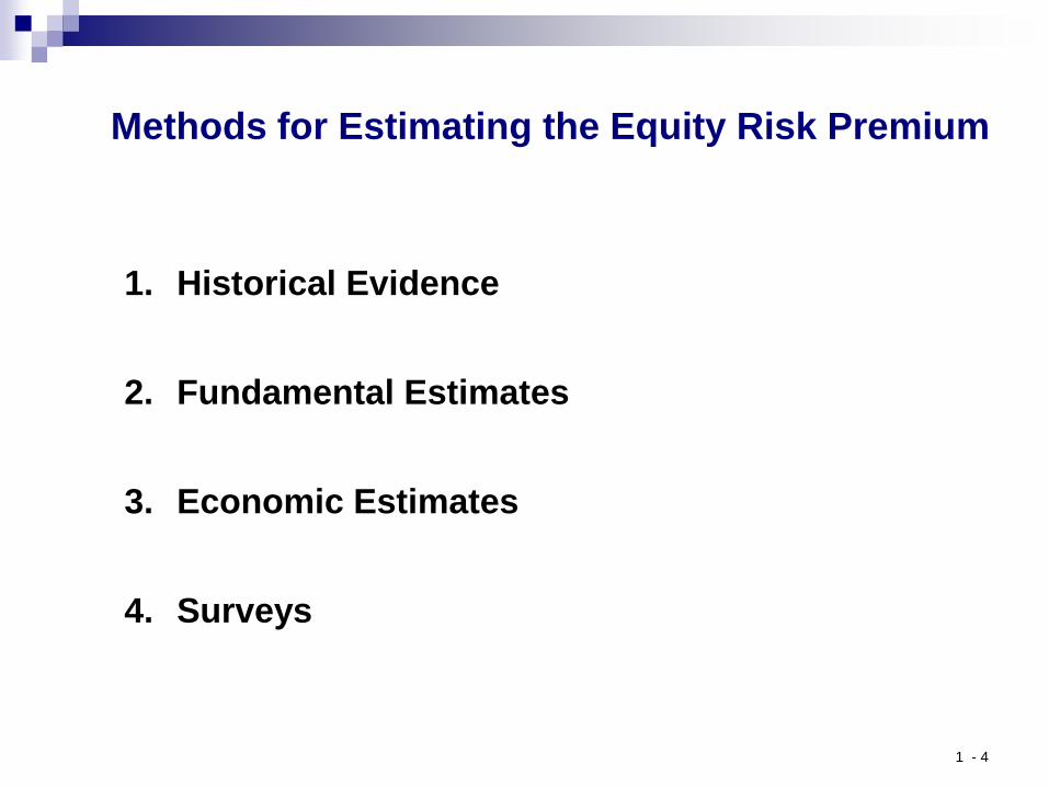
Methods for Estimating the Equity Risk Premium
1. Historical Evidence 2. Fundamental Estimates 3. Economic Estimates 4. Surveys
1 - 4
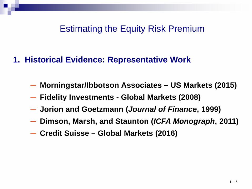
Estimating the Equity Risk Premium
1. Historical Evidence: Representative Work
– Morningstar/Ibbotson Associates – US Markets (2015) – Fidelity Investments - Global Markets (2008) – Jorion and Goetzmann (Journal of Finance, 1999) – Dimson, Marsh, and Staunton (ICFA Monograph, 2011) – Credit Suisse – Global Markets (2016)
1 - 5

1 - 6
Morningstar/Ibbotson Return & Risk Data: 1926 - 2015

Historical U.S. Nominal Asset Class Returns & Inflation:
1 - 7
Stocks:
Bonds:
T-Bills:
Inflation:
1926-2015: Avg. Return 11.95% 6.30% 3.45% 3.00% Std. Deviation 19.99% 8.42% 3.12% 4.09% 1991-2015: Avg. Return 11.43 8.37 2.75 2.32 Std. Deviation 18.13 8.54 2.19 1.00 2006-2015: Avg. Return 9.14 6.79 1.10 1.85 Std. Deviation 18.97 8.05 1.91 1.27
2011-2015: Avg. Return 13.11 7.56 0.04 1.53 Std. Deviation 12.64 11.18 0.02 0.97 Source: Morningstar/Ibbotson Associates

Historical U.S. Real Asset Class Returns & Equity Risk Premia:
1 - 8

U.S. Equity Risk Premium Histogram (vs. U.S. T-bills) There has been a wide disparity in annual realized risk premia over time and the
values are frequently negative
1 - 9

Illustrating the U.S. Equity Risk Premium: 1935 - 2015 (10-yr rolling avg. vs. Bills)
1 - 10
-10.00
-5.00
0.00
5.00
10.00
15.00
20.00
25.0019
3519
3719
3919
4119
4319
4519
4719
4919
5119
5319
5519
5719
5919
6119
6319
6519
6719
6919
7119
7319
7519
7719
7919
8119
8319
8519
8719
8919
9119
9319
9519
9719
9920
0120
0320
0520
0720
0920
1120
1320
15
Rolling 10-yr Avg USRisk PremiumLong-Term Avg
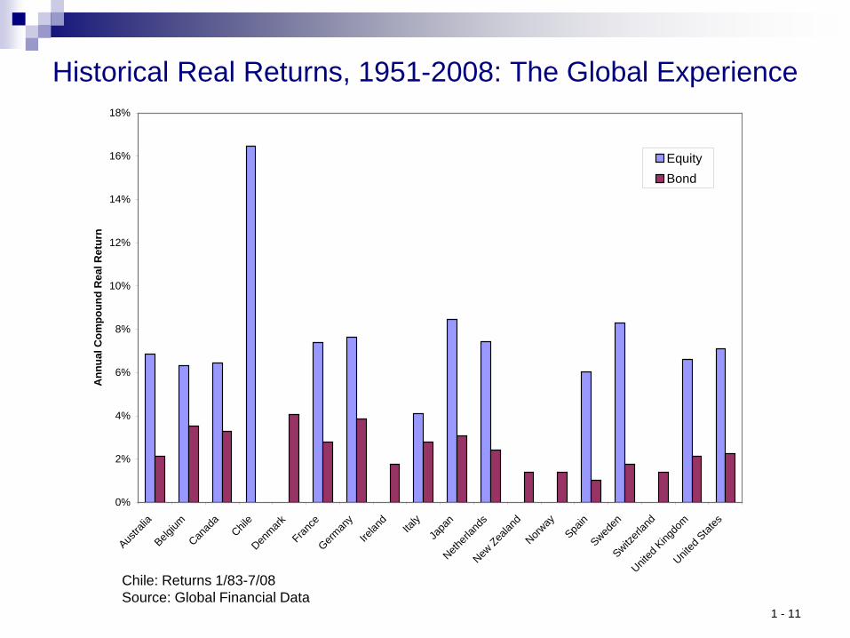
Historical Real Returns, 1951-2008: The Global Experience
Chile: Returns 1/83-7/08 Source: Global Financial Data
0%
2%
4%
6%
8%
10%
12%
14%
16%
18%
Austra
lia
Belgium
Canad
aChil
e
Denmark
France
German
y
Irelan
dIta
lyJa
pan
Netherl
ands
New Zea
land
Norway
Spain
Sweden
Switzerl
and
United
Kingdo
m
United
States
Ann
ual C
ompo
und
Rea
l Ret
urn
EquityBond
1 - 11

Historical Risk Premia, 1951-2008
-2%
0%
2%
4%
6%
8%
10%
12%
14%
Austra
lia
Belgium
Canad
aChil
e
Denmark
France
German
y
Irelan
dIta
lyJa
pan
Netherl
ands
New Zea
land
Norway
Spain
Sweden
Switzerl
and
United
Kingdo
m
United
States
Ris
k Pr
emia
(Geo
met
ric)
Equity-CashBond-Cash
Chile: Returns 1/83-7/08 Source: Global Financial Data
1 - 12

Historical Volatility Measures, 1951-2008
0%
5%
10%
15%
20%
25%
Austra
lia
Belgium
Canad
aChil
e
Denmark
France
German
y
Irelan
dIta
lyJa
pan
Netherl
ands
New Zea
land
Norway
Spain
Sweden
Switzerl
and
United
Kingdo
m
United
States
Ann
ual S
tand
ard
Dev
iatio
n
EquityBond
Chile: Returns 1/83-7/08 Source: Global Financial Data
1 - 13

Historical Global Equity Risk Premiums: 1900-2010
1 - 14

Illustrating the United Kingdom Equity Risk Premium (10-yr rolling avg. vs. Bills)
Source: Elroy Dimson, London Business School
1 - 15

Historical Global Equity Risk Premia: 1900 - 2015
1 - 16

Estimating the Equity Risk Premium (cont.)
2. Fundamental Estimates: Representative Work
– Fama and French (University of Chicago, 2000) – Ibbotson and Chen (Yale University, 2001) – Claus and Thomas (Journal of Finance, 2001) – Arnott and Bernstein (Financial Analysts Journal, 2002) – Mehra and Prescott (Hnbk Econ Fin, 2003) – Heaton and Lucas (Hnbk ERP, 2008) – Bloomberg Consensus Forecasts (2016)
1 - 17

Fundamental Risk Premium Estimates: An Overview
One potential problem with using historical averages to estimate future expected returns is that there is no way to control for the possibility that the past data sample you selected produced averages that are “abnormal” (i.e., too high or too low) in some way.
Another problem we have seen is that historical average returns tend to be fairly unstable (i.e., they are extremely sensitive to the time period chosen in the analysis).
Fundamental risk premium estimates attempt to objectively forecast
the expected returns that would normally occur, given the fundamental relationships that tend to exist in the capital markets. - In other words, fundamental forecasts attempt to link return expectations to
the economic conditions likely to pertain in the market during the forecast interval.
1 - 18

Fama and French: The Equity Risk Premium
Main Idea: Use dividend and earnings growth rates to measure the expected rate of capital gains for equity investments. This process creates two ways of then estimating real (i.e., inflation-adjusted) expected equity returns: - E(R) = E(Div Yld) + E(Real Growth Rate of Dividends) = RD - E(R) = E(Div Yld) + E(Real Growth Rate of Earnings) = RY
Notice that the intuition behind this approach is simply that it is possible to compensated investors in two ways: cash flow and capital gain. This is sometimes referred to as a demand-side approach to estimating the risk premium
Real Equity Risk Premium can then be estimated by subtracting short-term commercial paper yields from RD and RY, which leaves RXD and RXY, respectively
Main Result: Using data from the period 1951 to 2000 for the US market (i.e., S&P
500), they find that: - RXD = 2.55% - RXY = 4.32%
Notice that both of these fundamental risk premium estimates are well below the
average historical risk premium during the period (i.e., 7.43%), leading the authors that future expected returns to equity investments are unlikely to match the high levels of the recent past
1 - 19

Fama and French: The Equity Risk Premium (cont.)
1 - 20
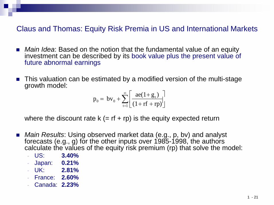
Claus and Thomas: Equity Risk Premia in US and International Markets
Main Idea: Based on the notion that the fundamental value of an equity investment can be described by its book value plus the present value of future abnormal earnings
This valuation can be estimated by a modified version of the multi-stage growth model:
where the discount rate k (= rf + rp) is the equity expected return
Main Results: Using observed market data (e.g., p, bv) and analyst
forecasts (e.g., g) for the other inputs over 1985-1998, the authors calculate the values of the equity risk premium (rp) that solve the model:
- US: 3.40% - Japan: 0.21% - UK: 2.81% - France: 2.60% - Canada: 2.23%
∑∞
=
++
++=
1t
t00 rp) rf (1
)gae(1 bv p
1 - 21
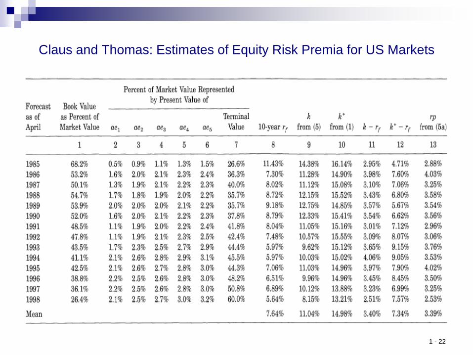
Claus and Thomas: Estimates of Equity Risk Premia for US Markets
1 - 22

Arnott and Bernstein: What Risk Premium is “Normal”?
Main Idea: The risk premium for stocks relative to bonds can be forecast as the difference between the expected real stock return and the expected real bond return. This is sometimes called a supply-side estimation process.
The real return to stocks consists of three components: - Dividend yield - Growth rate in the real dividend - Change in equity valuation level (e.g., change in market P/E)
The real return to bonds consists of three components:
- Nominal yield - Inflation - Change in yield times duration (i.e., reinvestment)
Main Conclusions:
- Historical real stock returns and the excess return for stocks relative to bonds over the past century have extraordinarily high (due to rising valuation multiples) and unlikely to be repeated in the future. The fundamental expected risk premium estimate over this past period would have been 2.4%
- Future expectations should be based on tractable fundamental relationships and indicate a real risk premium of near 0%
1 - 23

Arnott and Bernstein: What Risk Premium is “Normal”? (cont.)
1 - 24

Arnott and Bernstein: What Risk Premium is “Normal”? (cont.) Source: A. Ilmanen, Expected Returns on Major Asset Classes, CFA Institute, 2012
1 - 25
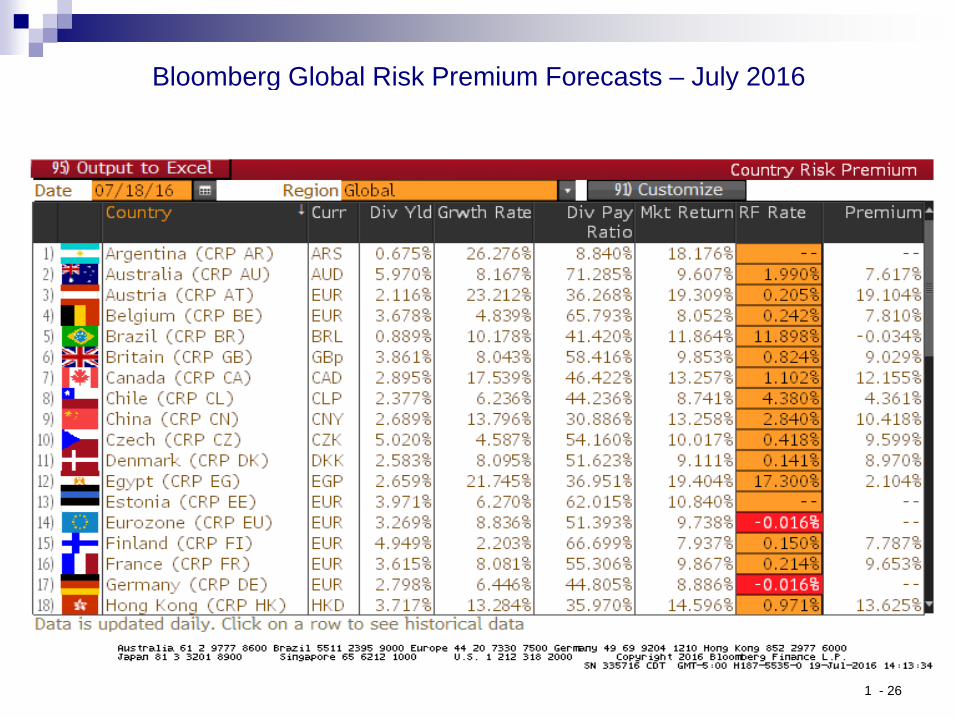
Bloomberg Global Risk Premium Forecasts – July 2016
1 - 26

Bloomberg Risk Premium Forecasts: 2014-2016 – United States
1 - 27

Bloomberg Risk Premium Forecasts: 2014-2016 – Chile
1 - 28
Estimating the Equity Risk Premium (cont.)
3. Economic Estimates: Representative Work
– Black and Litterman (1992, 2016) – Asset Class-Specific Risk Premia
– Aon Hewitt (2010, 2012)
– Damodaran (2015) – Country-Specific Risk Premia
1 - 29

Implied Returns and the Black-Litterman Forecasting Process
The Black-Litterman (BL) model uses a quantitative technique known as reverse optimization to determine the implied returns for a series of asset classes that comprise the investment universe.
The main insight of the BL model is that if the global capital markets are in equilibrium, then the prevailing market capitalizations of these asset classes suggest the investment weights of an efficient portfolio with the highest Sharpe Ratio (i.e., risk premium per unit of risk) possible.
These investment weights can then be used, along with information about asset class standard deviations and correlations, to transform the user’s forecast of the global risk premium into asset class-specific risk premia (and expected returns) that are consistent with a capital market that is in equilibrium.
1 - 30

1 - 31
4. Implied Expected Returns, Optimization, and TAA in the Black-Litterman Forecasting Process
The Black-Litterman (BL) model uses a quantitative technique known as reverse optimization to determine the implied returns for a series of asset classes that comprise the investment universe.
The main insight of the BL model is that if the global capital markets are in equilibrium, then the prevailing market capitalizations of these asset classes suggest the investment weights of an efficient portfolio with the highest Sharpe Ratio (i.e., risk premium per unit of risk) possible.
These investment weights can then be used, along with information about asset class standard deviations and correlations, to transform the user’s forecast of the global risk premium into asset class-specific risk premia (and expected returns) that are consistent with a capital market that is in equilibrium.
These equilibrium expected returns for the asset classes can then be used as inputs in a mean-variance portfolio optimization process or adjusted further given the user’s tactical views on asset class performance.
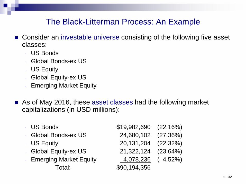
The Black-Litterman Process: An Example
Consider an investable universe consisting of the following five asset classes: - US Bonds - Global Bonds-ex US - US Equity - Global Equity-ex US - Emerging Market Equity
As of May 2016, these asset classes had the following market capitalizations (in USD millions):
- US Bonds $19,982,690 (22.16%) - Global Bonds-ex US 24,680,102 (27.36%) - US Equity 20,131,204 (22.32%) - Global Equity-ex US 21,322,124 (23.64%) - Emerging Market Equity 4,078,236 ( 4.52%) Total: $90,194,356
1 - 32
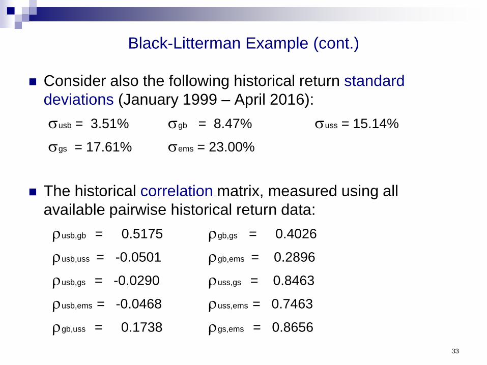
Black-Litterman Example (cont.)
Consider also the following historical return standard deviations (January 1999 – April 2016): σusb = 3.51% σgb = 8.47% σuss = 15.14%
σgs = 17.61% σems = 23.00%
The historical correlation matrix, measured using all available pairwise historical return data: ρusb,gb = 0.5175 ρgb,gs = 0.4026
ρusb,uss = -0.0501 ρgb,ems = 0.2896
ρusb,gs = -0.0290 ρuss,gs = 0.8463
ρusb,ems = -0.0468 ρuss,ems = 0.7463
ρgb,uss = 0.1738 ρgs,ems = 0.8656 33

Black-Litterman Example (cont.)
The remaining inputs that the user must specify are: (i) the global risk premium of the investment universe, and (ii) the risk-free rate. Using current market data we have:
- Global Risk Premium: 4.41% (10-yr Global Balanced) - Risk-Free Rate: 1.81% (10-yr US Treasury)
The heart of the BL process is to then calculate the implied
excess return for each asset class, using the following (stylized) formula:
[Risk Aversion Parameter] x [Covariance Matrix] x [Market Cap Weight Vector]
34

Black-Litterman Example (cont.)
The risk aversion parameter is the rate at which more return is required as compensation for more risk. It is calculated as:
RAP = [Global Risk Premium] / [Market Portfolio Variance]
It can be shown in this example that the market portfolio variance is (9.25%)2 = 0.856%, so that:
RAP = (0.0441)/(0.00856) = 5.15
The covariance between two asset classes (Y and Z) is given by the formula:
Cov(Y,Z) = ρy,z x σy x σz
For instance, the covariance between US Equity and Global Equity-ex US is: (0.8463) x (15.14%) x (17.61%) = 0.023
35

Black-Litterman Example (cont.)
The implied excess return (IER) for US Equity can then be computed as follows:
IERuss = (RAP) x {[Cov(uss,usb) x wusb] + [Cov(uss,gb) x wgb] +
… + [Cov(uss,ems) x wems]}
= (5.15) x {(0.000)(.2216) + … + (0.026)(.0452)} = 6.27% More formally, the solution for the entire asset class implied excess return
vector is given by:
0.30% 0.001 0.002 0.000 0.000 0.000 22.16% 2.31% 0.002 0.007 0.002 0.006 0.006 27.36% 6.27% = (5.15) x 0.000 0.002 0.023 0.022 0.026 x 22.32% 8.02% 0.000 0.006 0.023 0.031 0.035 23.64% 9.24% 0.000 0.006 0.026 0.035 0.053 4.52%
36

Black-Litterman Example (cont.)
The total expected return for US Equity is then simply the
IER plus the risk-free rate: 1.81% + 6.27% = 8.08%
The excess and total expected returns for the five asset
classes in this example are:
Excess Total - US Bonds: 0.30% 2.11% - Global Bonds: 2.31% 4.12% - US Equity: 6.27% 8.08% - Global Equity: 8.02% 9.83% - Emerging Equity: 9.24% 11.05%
37

Black-Litterman Example: Excel Spreadsheet
1 - 38

Black-Litterman Example: Proprietary Software (Zephyr Associates)
1 - 39

Aon Hewitt (AON)
Historically, AON has used a similar process to the BL methodology in that they develop asset class expected return forecasts that are grounded in the notion that the global capital markets are in equilibrium
Specifically, AON estimates asset class expected returns to be consistent with a global Capital Asset Pricing Model (CAPM). Two expected return “anchors” are used as a starting point: - US Equity = 7.0%: Total return is divided into three components:
dividend yield (1.8%), nominal growth rate of corporate earnings (5.2%), and change in valuation levels (0.0%)
- US Bonds = 4.6%: Based on two components: current yield and simulated future changes in yields (based on forecasts of expected inflation, inflation risk premium, and real yields)
1 - 40

AON Forecasts – March 2012
i - 41
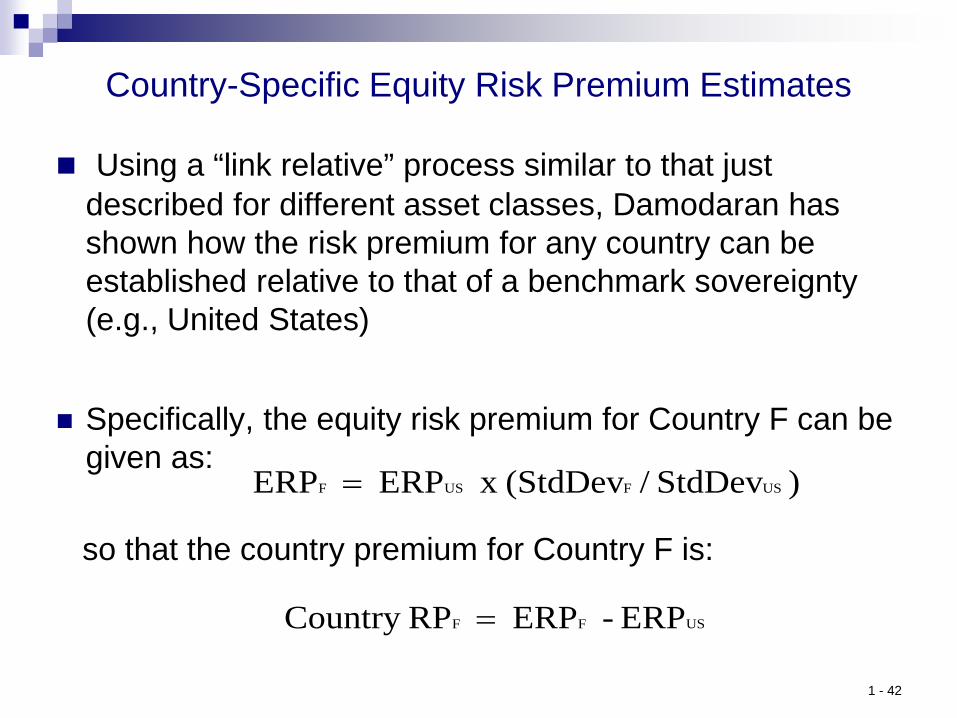
Country-Specific Equity Risk Premium Estimates
Using a “link relative” process similar to that just described for different asset classes, Damodaran has shown how the risk premium for any country can be established relative to that of a benchmark sovereignty (e.g., United States)
Specifically, the equity risk premium for Country F can be given as:
so that the country premium for Country F is: 1 - 42
) StdDev / (StdDev x ERP ERP USFUSF =
ERP - ERP RPCountry USFF =

Country-Specific Equity Risk Premium Estimates (cont.)
For example, over a recent two-year period, we observed the following data in the US and Chilean equity markets:
- ERPUS = 5.80% - StdDevUS = 17.67% - StdDevChile = 14.14%
So, for Chile:
and:
1 - 43
4.64% 17.67%) / (14.14% x 5.80% ERPChile ==
1.16%- 5.80% - 4.64% RPCountry Chile ==

Country-Specific Equity Risk Premium Estimates (cont.)
For various countries in Latin America as February 2015, Damodaran reports the following figures:
1 - 44

Estimating the Equity Risk Premium (cont.)
4. Surveys: Representative Work
– Graham and Harvey (Duke University, 2014) – Aon Hewitt : Managers & Consultants (2009) – Teacher Retirement System of Texas (2014) – Fernandez, Ortiz, Arcin (IESE Business School, 2016) – Bloomberg Consensus Forecasts (2016)
1 - 45

Graham-Harvey Survey of Corporate CFOs – April 2014
1 - 46

Graham-Harvey Survey – April 2014 (cont.)
1 - 47

Fernandez et al Global Analyst Survey – May 2016
1 - 48

Fernandez et al Global Analyst Survey – May 2016 (cont.)
1 - 49

Long-Term Expected Return & Volatility Forecasts: June 2014 (Texas Teacher Retirement System)
1 - 50

Long-Term Risk Premium Forecasts: June 2014 (Texas Teacher Retirement System)
1 - 51
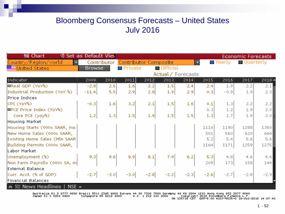
Bloomberg Consensus Forecasts – United States July 2016
1 - 52

Bloomberg Consensus Forecasts – Euro Region July 2016
1 - 53

Bloomberg Consensus Forecasts – Chile July 2016
1 - 54

The Equity Risk Premium: Some Concluding Thoughts The equity risk premium represents the crucial component to predicting
expected returns for stockholders, which impact everything from forecasting future market conditions to security valuation to measuring portfolio performance
There is no clear-cut best way to forecast equity risk premia - Extrapolating historical trends, forming an economically justifiable prediction, and
surveying other market participants are all used frequently in practice
There is a big disparity between the theoretical and historical levels of the equity risk premium - This gap between what theory predicts and what the actual data have shown is
called the equity premium puzzle, which has been the subject a substantial research literature attempting to explain it
Measured equity risk premia vary widely across different economies as well
as over time within any particular economy - This makes relying on a single point estimate at a specific point in time challenging
Equity risk premia throughout the world have been negative for the most
recent historical rolling-average periods, meaning that this data seems to be of relatively little use in helping us understand what to expect in the future
1 - 55


