The Equivalence of the Radial Return and Mendelson … · Steven M. Arnold Glenn Research Center...

Brett A. Bednarcyk and Jacob Aboudi

Ohio Aerospace Institute, Brook Park, Ohio

Steven M. Arnold

Glenn Research Center, Cleveland, Ohio

The Equivalence of the Radial Return and

Mendelson Methods for Integrating the Classical

Plasticity Equations

NASA/TM—2006-214331

July 2006

https://ntrs.nasa.gov/search.jsp?R=20060045066 2018-07-29T02:50:46+00:00Z

NASA STI Program . . . in Profile

Since its founding, NASA has been dedicated to the

advancement of aeronautics and space science. The

NASA Scientific and Technical Information (STI)

program plays a key part in helping NASA maintain

this important role.

The NASA STI Program operates under the auspices

of the Agency Chief Information Officer. It collects,

organizes, provides for archiving, and disseminates

NASA’s STI. The NASA STI program provides access

to the NASA Aeronautics and Space Database and its

public interface, the NASA Technical Reports Server,

thus providing one of the largest collections of

aeronautical and space science STI in the world.

Results are published in both non-NASA channels and

by NASA in the NASA STI Report Series, which

includes the following report types:

• TECHNICAL PUBLICATION. Reports of

completed research or a major significant phase

of research that present the results of NASA

programs and include extensive data or theoretical

analysis. Includes compilations of significant

scientific and technical data and information

deemed to be of continuing reference value.

NASA counterpart of peer-reviewed formal

professional papers but has less stringent

limitations on manuscript length and extent of

graphic presentations.

• TECHNICAL MEMORANDUM. Scientific

and technical findings that are preliminary or

of specialized interest, e.g., quick release

reports, working papers, and bibliographies that

contain minimal annotation. Does not contain

extensive analysis.

• CONTRACTOR REPORT. Scientific and

technical findings by NASA-sponsored

contractors and grantees.

• CONFERENCE PUBLICATION. Collected

papers from scientific and technical

conferences, symposia, seminars, or other

meetings sponsored or cosponsored by NASA.

• SPECIAL PUBLICATION. Scientific,

technical, or historical information from

NASA programs, projects, and missions, often

concerned with subjects having substantial

public interest.

• TECHNICAL TRANSLATION. English-

language translations of foreign scientific and

technical material pertinent to NASA’s mission.

Specialized services also include creating custom

thesauri, building customized databases, organizing

and publishing research results.

For more information about the NASA STI

program, see the following:

• Access the NASA STI program home page at

http://www.sti.nasa.gov

• E-mail your question via the Internet to

[email protected]

• Fax your question to the NASA STI Help Desk

at 301–621–0134

• Telephone the NASA STI Help Desk at

301–621–0390

• Write to:

NASA STI Help Desk

NASA Center for AeroSpace Information

7121 Standard Drive

Hanover, MD 21076–1320

The Equivalence of the Radial Return and

Mendelson Methods for Integrating the Classical

Plasticity Equations

NASA/TM—2006-214331

July 2006

National Aeronautics and

Space Administration

Glenn Research Center

Cleveland, Ohio 44135


Ohio Aerospace Institute, Brook Park, Ohio

Steven M. Arnold

Glenn Research Center, Cleveland, Ohio

Available from

NASA Center for Aerospace Information

7121 Standard Drive

Hanover, MD 21076–1320

National Technical Information Service

5285 Port Royal Road

Springfield, VA 22161

Available electronically at http://gltrs.grc.nasa.gov

This work was sponsored by the Fundamental Aeronautics Program

at the NASA Glenn Research Center.

Level of Review: This material has been technically reviewed by technical management.

NASA/TM—2006-214331 1

The Equivalence of the Radial Return and Mendelson Methods for Integrating the Classical Plasticity Equations


Ohio Aerospace Institute Brook Park, Ohio 44142

Steven M. Arnold

National Aeronautics and Space Administration Glenn Research Center Cleveland, Ohio 44135

Abstract The radial return and Mendelson methods for integrating the equations of classical plasticity, which

appear independently in the literature, are shown to be identical. Both methods are presented in detail as are the specifics of their algorithmic implementation. Results illustrate the methods’ equivalence across a range of conditions and address the question of when the methods require iteration in order for the plastic state to remain on the yield surface. FORTRAN code implementations of the radial return and Mendelson methods are provided in the appendix.

1. Introduction With the advent of modern computers and commercial finite element analysis (FEA) codes, the

inelastic analysis of structures is economical and accessible to design engineers. Accounting for inelasticity is critical in today’s simulation-based design paradigm in order to capture the true nature of the structural response. This is particularly true in the case of aerospace structures where weight is the driving design parameter. Allowing local inelastic deformation of materials provided the effects of this deformation can be accurately modeled and shown to be safe, can increase design efficiency by minimizing overly conservative designs intended to stave off yielding. As such, mathematical models that treat inelastic deformation of materials have become increasingly important over the last 50 years. Obviously, metallic materials are the primary application of such models. However, polymers and other non-metallic materials that exhibit permanent deformation are beneficiaries of plasticity models as well.

The basic structural problem of interest is the boundary value problem consisting of a specified structural geometry along with specified loading acting on the structure. The goal is to determine the stress, deformation, and strain distribution throughout the structure, which is accomplished through solution of the equilibrium equations while enforcing the boundary conditions, compatibility, and the constitutive relations for the material. In the general, nonlinear case, initial conditions must be specified and, because the problem may be time/history dependent, the solution must be accomplished through incremental and/or iterative methods. As mentioned above, FEA codes provide a convenient means to solving such problems, although many useful structural problems can still be addressed via conventional analytical methods.

This paper addresses one part of the above posed general boundary value problem; namely, the constitutive relations for the material. Equally applicable to FEA and conventional analytical solutions, it will be assumed herein that the constitutive relations in question are active at a point within a structure and that the structure-scale solution satisfies the equilibrium equations, compatibility, and the specified boundary conditions. The problem of interest thus reduces to:

NASA/TM—2006-214331 2

• Given an admissible specified stress/strain state at a given location • Determine the unspecified stress/strain components at that location

For instance, in the case of FEA, it is the role of the finite element method to ensure that the equilibrium and compatibility equations are satisfied. At a given element integration point and a given loading step, n, for a given strain increment, Δε, the problem of interest becomes determination of the new stress state at the integration point for loading step n+1. This obviously assumes that the converged state is known completely at step n.

We now further restrict ourselves to the quasi-static (i.e., non-dynamic) and small deformation regimes and concentrate on rate-independent classical plasticity. Classical plasticity is popular due to its simplicity and ease of characterization. In the case of isotropic hardening, a single stress-strain curve is all that is required to characterize the classical plasticity parameters. Obviously, this simplicity limits its accuracy, but classical plasticity does capture the first-order effects of the plastic phenomenon and is quite useful in many instances. Classical plasticity employs a yield function, which describes the onset of plasticity, and an associated flow rule, which dictates the evolution of the plastic strain components. In some cases, local iterations are necessary in order to ensure that the stress state remains on the yield surface during plastic deformation. These iterations are independent of any global iterations required to solve the structural problem and are needed so that the correct local stress/strain state (at a point in the structure) are determined.

The algorithmic implementation of the classical plasticity equations, their integration, and the need for the above-mentioned local iterations are the main focus of this paper. We consider two sources/methods that describe classical plasticity equation integration. The first is the monograph by Mendelson (1968, 1983). Mendelson’s integration method has been employed by the present authors for a number of years in a series of non-FEA based micromechanics theories and codes for the inelastic response of composite materials. The second is the so-called “radial return method” (Simo and Taylor, 1985; Simo and Hughes, 1998), which appears to be much more popular and well-known than Mendelson’s method. The motivation for this investigation was to determine whether some advantage (computational or otherwise) could be gained by employing the radial return method rather than Mendelson’s method, given the popularity of the former. As will be shown, such an advantage was not found because the methods are, in fact, equivalent. While it is not the intent of this paper to attempt to discern which method arose first, we note that the roots of the radial return method are generally attributed to Wilkins (1964). However, it appears that both methods were developed independently.

Restricting the discussion to isotropic hardening (both linear and nonlinear), we begin by presenting in detail the radial return and Mendelson methods, including details of the integration algorithms. Next the two methods are explicitly shown to be equivalent. Note that this equivalence is summarized in tables 1 and 2 via side by side comparisons of the steps involved in the two methods. Results applicable to a monolithic (unreinforced) elastoplastic material are then presented for the two methods to indicate the methods’ equivalence while investigating the role of the local iteration procedure. Finally, results are presented for a composite material whose matrix material is treated as elastoplastic within a micromechanics model developed by the present authors. It should be noted that explicit nonlinear isotropic hardening, which was included in the radial return method by Simo and Taylor (1985), has now been included within the Mendelson method. Mendelson’s (1968, 1983) hardening is restricted to the linear and piece-wise linear cases. In addition, the FORTRAN code for the radial return and Mendelson methods employed for the presented monolithic results is given in the appendix. This code, with some modification, is suitable for incorporation within an elastoplastic structural analysis code.

NASA/TM—2006-214331 3

TABLE 1.—STEP BY STEP SUMMARY COMPARISON OF THE RADIAL RETURN AND MENDELSON METHODS

Step Radial return method Mendelson method 1 Compute elastic trial stress from equation (6),

( )1 12+ += + −Tn n n nGs s e e

Compute elastic trial strain deviator (referred to as the modified total strain deviator by Mendelson), ′e , from equation (32), and the equivalent modified total strain, etε , from equation (37),

1p

n n+= −′e e ε 23et ij ije eε = ′ ′

2 Check the yield criterion, equation (10).

( )1 1 ,2( , ) 03+ +κ = − κ ε =

nT Tn n pf s s

If 1( , ) 0+ κ <Tnf s , set 1 1+ += T

n ns s , 1+ =p pnnε ε , and the increment

is completed. Otherwise, continue.

Check the yield criterion, which can be written as,

( ) ( ),, 0

3np

etfG

κ εκ = ε − =′e

If ( ), 0<′f κe , set 1 2+ = ′n Gs e , 1+ =p pnnε ε , and the increment

is completed. Otherwise, continue. 3 Calculate the unit normal vector,

1 1ˆ + += T Tn nn s s

and determine the value of tγΔ from equation (17),

( )11 ,22 03 n

Tn pG t

++ − γΔ − κ ε =s

In the case of linear hardening, the result is, ( )1 ,2 3

2 2 3n

Tn pY H

tG H

+ − + εγΔ =

+

s , =−

T

T

E EH

E E

see table 2 for the nonlinear hardening case.

Calculate the modified proportionality constant, Δ ′λ , from equation (52),

( )1,1

3np

etG+

κ εΔλ = −′

ε

In the case of linear hardening, the result is, ,1 1

1 3 3np

et

Y HH G G

+ ε⎡ ⎤Δλ = −′ ⎢ ⎥+ ε⎢ ⎥⎣ ⎦

see table 2 for the nonlinear hardening case.

4 Compute the equivalent plastic strain at increment n+1 from equation (6) as follows,

1, , 2 3n np p t+

ε = ε + γΔ (18)

and the plastic strain components from equation (5) as follows,

1 ˆp pnn t+ = + γΔε ε n (19)

Compute the equivalent plastic strain at increment n+1 from equation (41),

1, ,n np p et+ε = ε + Δλ ε′


1p p

nn+ = + Δλ′ ′ε ε e

5 If the hardening is nonlinear, check for global convergence by comparing the values of 1+ns determined from the yield function (1) and from the constitutive equation (7),

( )11 ,23 n

YFn p ++ = κ εs (20)

( ) ( )1 , 1 , 1 , 1 , 12 p pCn ij n n ij n nij ijG e e+ + + + += − ε − εs (21)

If 1 1+ +− >YF Cn n TOLs s go to step 3. Note that in the case of

linear hardening with loading that is not completely applied strains (i.e., blended loading), an additional convergence criterion is needed to ensure that the applied

1+ns is equal to 1+YFns and 1+

Cns .

If the hardening is nonlinear, check for global convergence by comparing the value of 1n+σ determined from the yield function, ( )11 , 0

nn p ++σ −κ ε = , to the value of

1n+σ determined from the constitutive equation (7),

( )11 ,nYFn p ++σ =κ ε (69)

( ) ( )1 , 1 , 1 , 1 , 1322

p pCn ij n n ij n nij ijG e e+ + + + +σ = − ε − ε (70)

If 1 1YF Cn n TOL+ +σ − σ > go to step 2. Note that in the case of

linear hardening with loading the is not completely applied strains, an additional convergence criterion is needed to ensure that the applied 1n+σ is equal to 1

YFn+σ and

1Cn+σ .

6 If necessary, calculate the deviatoric stress fromequation (11) or equation (4),

( )11 ,2 ˆ3 nn p ++ = κ εs n or ( )1 1 12+ + += − p

n n nGs e ε

If necessary, calculate the deviatoric stresses from equation (68) or equation (7),

( )11 ,23 nn p

et++

′= κ ε

εes or ( )1 1 12 p

n n nG+ + += −s e ε

NASA/TM—2006-214331 4

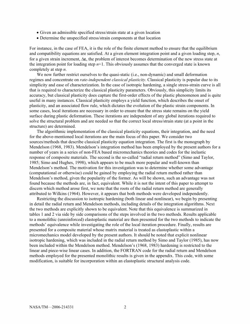
TABLE 2.—STEP BY STEP SUMMARY COMPARISON OF THE RADIAL RETURN AND MENDELSON METHOD PROCEDURE FOR DETERMINING γΔt AND Δλ′ IN THE CASE OF NONLINEAR HARDENING

NEEDED IN STEP 4 OF TABLE 1.

Step Radial return method Mendelson method 1 Calculate for iteration k,

( )1 1

1, , 2 3

n n

kk kp p t

+ +

+ε = ε + γΔ Calculate for iteration k,

( )1, 1 , 1

kk kp n p n et++ +ε = ε + Δλ ε′

2 Calculate the derivative of the function g (with respect to tγΔ ), as follows (see section 2.2 for details),

( )

( ) ( )1

, ,

2

2 3 2 3n n

Tn

p p

g t G t

t

+γΔ = − γΔ −

⎡ ⎤κ ε + γΔ κ ε′⎣ ⎦

s

( ),2 23 npg G= − κ ε −′ ′

Calculate the derivative of the function g (with respect to Δλ′ ), as follows (see section 4.2 for details),

( ) ( ) ( ), ,1

3 n np et pet

g G G⎡ ⎤Δλ = − κ ε + Δλ ε κ ε − Δλ′ ′ ′ ′⎣ ⎦ε

( ),13 npg G= − κ ε −′ ′

3 By the Newton-Raphson method,

( ) ( )( )

( )1

kk k

k

g tt t

g t

+⎡ ⎤γΔ⎢ ⎥⎣ ⎦γΔ = γΔ −⎡ ⎤γΔ′ ⎢ ⎥⎣ ⎦

By the Newton-Raphson method,

( ) ( )( )

( )1

kk k

k

g

g+

⎡ ⎤Δλ′⎢ ⎥⎣ ⎦Δλ = Δλ −′ ′⎡ ⎤Δλ′ ′⎢ ⎥⎣ ⎦

4 If ( ) TOLkg t⎡ ⎤γΔ >⎢ ⎥⎣ ⎦ then k → k+1, go to (1) If ( ) TOLkg ⎡ ⎤Δλ >′⎢ ⎥⎣ ⎦

then k → k+1, go to (1)

2. Radial Return Method Let us define the von Mises yield criterion with isotropic strain hardening as follows,

( )2( , ) 03

κ ≡ − κ ε =pf s s (1)

where s is the deviator of the stress σ, namely,

13

= σ − σ δij ij kk ijs (2)

and δij is the Kronecker delta. Note that for convenience and clarity, a mix of vector and indicial notation will be employed. In equation (1), the norm of s is given by,

22= =ij ijs s Js (3)

where J2 is the second invariant of s. In addition, ( )κ εp is the isotropic strain hardening rule, which

depends on the equivalent plastic strain:

23

ε = Δε = Δε Δε∫ ∫ p pp p ij ij (4)

where ε p

ij are the plastic strain components and Δ indicates an increment, which may accumulate between step n and step n+1 of the imposed loading profile. The flow rule is given by,

NASA/TM—2006-214331 5

ˆ∂Δε = γΔ = γΔ

∂pij

ij

ft ts

n (5)

where n̂ is the unit vector, ˆ =n s s , and γΔt is the magnitude of the plastic strain increment, which is in keeping with the nomenclature of Simo and Taylor (1985).

Substituting equation (5) into equation (4) yields,

23

Δε = γΔp t (6)

The deviatoric nature of the plastic strain allows the constitutive equation for isotropic elastoplastic

materials to be written as,

( )2= − pGs e ε (7)

where G is the shear modulus and e is the deviator of the total strain ε,

13

= ε − ε δij ij kk ije (8)

According to the radial return mapping algorithm, at the current increment, n, we assume an elastic trial stress applicable to the next increment, n+1,

( )1 12+ += + −T

n n n nGs s e e (9)

where 1+ne is the deviatoric strain at the next increment. This deviatoric strain may be known exactly, as in the case of pure strain specified loading on the material, it may be derived from blended stress/strain loading on the material, or it may be passed to the plasticity model from a higher scale model such as the finite element method. The radial return algorithm requires that the correct 1+ne is known or can be determined through a global iteration procedure.

From the yield criterion, equation (1), if

( ),1 12( , ) 03+ +κ = − κ ε <

nT Tn n pf s s (10)

then no yielding occurs (i.e., the deformation is elastic) and 1 1+ += T

n ns s . Otherwise, from equations (5) and (7), we have,

1 1 ˆ2+ +− −⎛ ⎞= − γ⎜ ⎟⎝ ⎠Δ Δn n n nG

t ts s e e n (11)

Substituting for ns in equation (11) using equation (9) we get,

NASA/TM—2006-214331 6

1 1 ˆ2+ += − γΔTn n G ts s n (12)

Since ˆ =n s s , we have, 1 1 ˆ+ +=n ns s n , and by substitution into equation (12), it can be shown that the

unit normal vector n̂ can be determined in terms of the trial elastic stress 1+Tns according to,

1 1ˆ + += T Tn nn s s . This fact is key to the radial return method because it indicates that the directionality of

the trial stress is identical to that of the converged stress, which is on the yield surface. It is therefore possible to return to the yield surface along this unit vector.

By multiplying equation (1) at increment n+1 by n̂ , we obtain,

( ), 112 ˆ3 ++

⎡ ⎤− κ ε =⎢ ⎥

⎣ ⎦nn ps n 0 (13)

Thus, from 1 1 ˆ+ +=n ns s n , it follows that,

( ), 112 ˆ3 ++ − κ ε =

nn ps n 0 (14)

From equation (12),

1 1 1ˆ ˆ ˆ2 2+ + +⎡ ⎤= − γΔ = − γΔ⎣ ⎦

T Tn n nG t G ts n s n n s (15)

Substituting equation (15) into equation (14), we obtain,

( ), 112 ˆ23 ++

⎡ ⎤− γΔ − κ ε =⎢ ⎥

⎣ ⎦n

Tn pG ts n 0 (16)

Hence, we will define the function ( )γΔg t as the bracketed term in equation (16), namely,

( ) ( )11 ,22 03 ++γΔ = − γΔ − κ ε =

nTn pg t G ts (17)

This nonlinear equation is used to determine the value of γΔt .

With the above equations, the formulation required to determine all variables at increment n+1 given their values at increment n has been completed. The radial return method can thus be summarized as follows (see also table 1):

(1) Compute elastic trial stress from equation (6),

( )1 12+ += + −T

n n n nGs s e e

(2) Check the yield criterion, equation (10). If 1( , ) 0+ κ <Tnf s , set 1 1+ += T

n ns s , 1+ =p pnnε ε , and the

increment is completed. Otherwise, continue.

NASA/TM—2006-214331 7

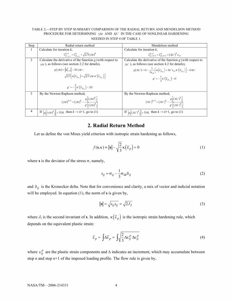
(3) Calculate the unit normal vector, 1 1ˆ + += T T

n nn s s

and determine the value of γΔt from equation (17). See sections 2.1 and 2.2 below for the linear and nonlinear hardening cases. (4) Compute the equivalent plastic strain at increment n+1 from equation (6) as follows,

1, ,

23+

ε = ε + γΔn np p t (18)

and the plastic strain components from equation (5) as follows, 1 ˆ+ = + γΔp p

nn tε ε n (19) (5) If the hardening is nonlinear, check for global convergence by comparing the value of 1+ns

determined from the yield function, equation (1), to the value of 1+ns determined from the constitutive equation (7). That is, the value of 1+ns from the yield function is given by,

( )11 ,23 ++ = κ ε

nYFn ps (20)

and the value of 1+ns from the constitutive equation (7) (utilizing eq. (3)) is,

( ) ( )1 , 1 , 1 , 1 , 12+ + + + += − ε − εp pCn ij n n ij n nij ijG e es (21)

If 1 1+ +− >YF C

n n TOLs s † go to step 3. Note that in the case of linear hardening with loading involving

anything other than six specified strain components, an additional convergence criterion is needed to ensure that the applied 1+ns is equal to 1+

YFns and 1+

Cns .

(6) If necessary, calculate the deviatoric stress from equation (14) or equation (7),

( )11 ,2 ˆ3 ++ = κ ε

nn ps n or ( )1 1 12+ + += − pn n nGs e ε

2.1 Linear Hardening

In the case of linear hardening, in which,

† It is suggested to use a TOL value that is a small fraction of 1+

Cns , such as 1TOL 0.0000001 C

n+= s .

NASA/TM—2006-214331 8

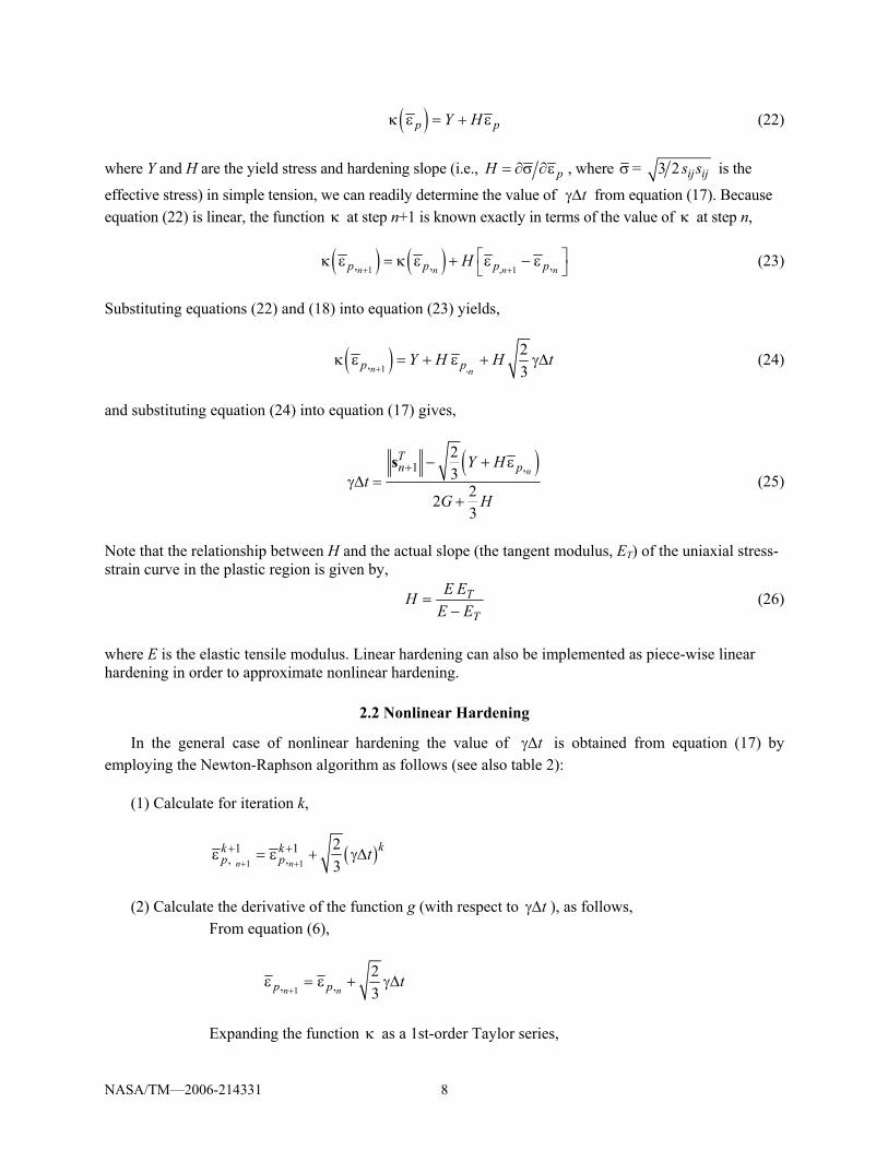
( )κ ε = + εp pY H (22)

where Y and H are the yield stress and hardening slope (i.e., = ∂σ ∂εpH , where σ= 3 2 ij ijs s is the

effective stress) in simple tension, we can readily determine the value of γΔt from equation (17). Because equation (22) is linear, the function κ at step n+1 is known exactly in terms of the value of κ at step n,

( ) ( )1 , 1, , ,+ +

⎡ ⎤κ ε = κ ε + ε − ε⎣ ⎦n n n np p p pH (23)

Substituting equations (22) and (18) into equation (23) yields,

( )1 ,,23+

κ ε = + ε + γΔn np pY H H t (24)

and substituting equation (24) into equation (17) gives,

( )1 ,

23

223

+ − + εγΔ =

+

nTn pY H

tG H

s (25)

Note that the relationship between H and the actual slope (the tangent modulus, ET) of the uniaxial stress-strain curve in the plastic region is given by,

=−

T

T

E EHE E

(26)

where E is the elastic tensile modulus. Linear hardening can also be implemented as piece-wise linear hardening in order to approximate nonlinear hardening.

2.2 Nonlinear Hardening

In the general case of nonlinear hardening the value of γΔt is obtained from equation (17) by employing the Newton-Raphson algorithm as follows (see also table 2):

(1) Calculate for iteration k,

( )1 1

1 1, ,

23n n

kk kp p t

+ +

+ +ε = ε + γΔ

(2) Calculate the derivative of the function g (with respect to γΔt ), as follows,

From equation (6),

1, ,

23+

ε = ε + γΔn np p t

Expanding the function κ as a 1st-order Taylor series,

NASA/TM—2006-214331 9

( ) ( ) ( )1, , , ,2 23 3+

⎛ ⎞κ ε = κ ε + γΔ = κ ε + γΔ κ ε′⎜ ⎟⎝ ⎠n n n np p p pt t

Hence, from equation (17),

( ) ( ) ( )1 , ,2 223 3+⎡ ⎤

γΔ = − γΔ − κ ε + γΔ κ ε′⎢ ⎥⎣ ⎦

n nTn p pg t G t ts

Therefore,

( ),2 23

= − κ ε −′ ′npg G

(3) By the Newton-Raphson method,

( ) ( )( )

( )1+

⎡ ⎤γΔ⎣ ⎦γΔ = γΔ −⎡ ⎤γΔ′ ⎣ ⎦

kk k

k

g tt t

g t

(4) If ( ) TOL⎡ ⎤γΔ >⎣ ⎦kg t ‡ then k → k+1, go to (1)

Let us illustrate the nonlinear hardening for the case in which the hardening function is given by,

( ) ( )e 1− εκ ε = − −pAp

HYA

(27)

where Y is the yield stress in simple tension and H and A are material parameters. Elastic-perfectly plastic material response is obtained when H = 0 and bilinear material response (i.e., linear hardening) is obtained when A is small (but not zero), yielding

( )κ ε = + εp pY H (28)

and we see that the parameter H is then the hardening slope. In the general case, H is the initial slope of the nonlinear portion of the material response. Finally, for large values of εp , the stress will saturate to a

value of Y + H/A. Note that the derivative, ( ),κ ε′np , needed in step 2 of the radial return procedure

above, is given by,

( ) ,, e− ε

κ ε =′ p nn

Ap H (29)

‡ A small value for the Newton-Raphson tolerance, such as 0.0001, is suggested.

NASA/TM—2006-214331 10

3. Mendelson Method Mendelson (1968) derived plastic strain – total strain plasticity relations, which enable the

computation of the plastic strain increments from total strains without recourse to the stresses. As in the radial return method, it is assumed that the load is incremented from a completely known state at increment n to the next increment n+1, with the task being to determine the state at this next increment in the context of classical plasticity. The strain at the next increment can thus be written as,

1 1+ += + + Δe p p

n n nε ε ε ε (30)

where the superscript “e” refers to an elastic quantity. Subtracting the mean strain ( 3ε = εmean kk ) from both sides of equation (30) yields,

1 1+ += + + Δe p p

n n ne e ε ε (31)

The Mendelson method defines the modified total strain deviator associated with the increment as,

1+= −′ pn ne e ε (32)

Combining equations (32) and (31),

1+= + Δ′ e p

ne e ε (33)

From Hooke’s law and the Prandtl-Reuss equations we have,

11 2 2

++

Δ= =

Δλ

pe nn G G

s εe (34)

where Δλ is the Prandtl-Reuss proportionality constant. Substituting equation (34) into equation (33),

112

⎛ ⎞= + Δ′ ⎜ ⎟Δλ⎝ ⎠

pG

e ε (35)

Multiplying both sides of equation (31) by 2/3 times itself,

2

2 2 113 3 2

⎛ ⎞= + Δε Δε′ ′ ⎜ ⎟Δλ⎝ ⎠

p pij ij ij ije e

G (36)

Mendelson defines the equivalent modified total strain as,

23

ε = ′ ′et ij ije e (37)

which, along with equation (4) allows the following equation to be written from equation (37),

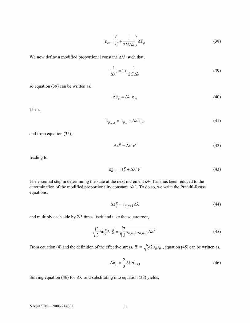
NASA/TM—2006-214331 11

112

⎛ ⎞ε = + Δε⎜ ⎟Δλ⎝ ⎠et pG

(38)

We now define a modified proportional constant Δλ′ such that,

1 112

= +Δλ Δλ′ G

(39)

so equation (39) can be written as,

Δε = Δλ ε′p et (40)

Then,

1, ,+ε = ε + Δλ ε′

n np p et (41)

and from equation (35),

Δ = Δλ′ ′pε e (42)

leading to,

1+ = + Δλ′ ′p p

nnε ε e (43)

The essential step in determining the state at the next increment n+1 has thus been reduced to the determination of the modified proportionality constant Δλ′ . To do so, we write the Prandtl-Reuss equations,

, 1+Δε = Δλp

ij nij s (44)

and multiply each side by 2/3 times itself and take the square root,

2, 1 , 1

2 23 3 + +Δε Δε = Δλp p

ij n ij nij ij s s (45)

From equation (4) and the definition of the effective stress, σ = 3 2 ij ijs s , equation (45) can be written as,

123 +Δε = Δλσp n (46)

Solving equation (46) for Δλ and substituting into equation (38) yields,

NASA/TM—2006-214331 12

113

+⎛ ⎞σ

ε = + Δε⎜ ⎟Δε⎝ ⎠n

et ppG

(47)

or,

13+σ

Δε = ε − np et G

(48)

Then, substituting equation (40) into equation (48), we have,

113

+σΔλ = −′

εn

etG (49)

where σ is taken from the yield function, i.e., for linear hardening, pY Hσ = + ε (50)

4. Equivalence of the Radial Return and Mendelson Methods It is now possible to show that the Mendelson method is exactly equivalent to the radial return

method. First, it follows from equation (1) (and can be clearly seen by comparing equation (50) to equation (22)), that Mendelson’s σ is equivalent to the function κ in the radial return method, which defines the material hardening law. That is,

( )σ = κ εp (51)

allowing equation (49) to be written as,

( )1,ε

λ 13 ε

+Δ = −′ np

etGκ

(52)

From the material elastoplastic constitutive equation (7), at the known increment n, we have,

( )2= − p

n n nGs e ε (53)

Substituting equation (53) into equation (9) and comparing to equation (32) yields,

( )1 12 2+ += − = ′T p

n n nG Gs e ε e (54)

and we see the equivalence between the role of the trial stress in the radial return method and the modified total strain deviator in the Mendelson method. The latter is, in fact, a strain-like trial quantity. This can be shown independently by considering equation (31) in the trial state, where the elastic strain deviator becomes the trial strain deviator and it is assumed that, in the trial condition, 0Δ =pε . Equation (31) can then be written as,

NASA/TM—2006-214331 13

1 1+ += +T pn n ne e ε (55)

where the trial strain deviator is denoted as 1+

Tne . Rearranging equation (55) and comparing to

equation (32), we have,

1 1+ += − = ′T pn n ne e ε e (56)

thus confirming that Mendelson’s modified total strain deviator is indeed a trial strain deviator in the sense of the radial return method.

From equations (54), (37), and (3),

( ) ( )1 1 12 6+ + +

= = = ε′ ′T T Tn ij ij ij ij etn n

s s G e e Gs (57)

which gives,

116 +ε = T

et nGs (58)

and we see that Mendelson’s equivalent modified total strain takes on a role analogous to that of the norm of the trial stress in the radial return method. We also note that the radial return method unit normal,

1 1ˆ + += T Tn nn s s , can be written in terms of Mendelson’s modified quantities using equations (54) and

(57) as,

2ˆ3

′=

εet

en (59)


( )1,

1

213

np

Tn

+

+

κ εΔλ = −′

s (60)

Comparing equation (18) with equation (41), we have,

23

Δλ ε = γΔ′ et t (61)

Substituting equations (58) and (60) into equation (61) gives,

( ), 1

11

2 1 213 36

np TnT

nt

G+

++

⎡ ⎤κ ε⎢ ⎥− = γΔ⎢ ⎥

⎢ ⎥⎣ ⎦

ss

(62)

NASA/TM—2006-214331 14

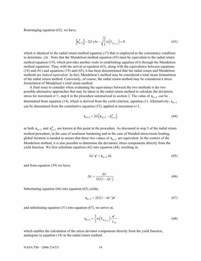
Rearranging equation (62), we have,

( ), 1122 03 ++ − γΔ − κ ε =

nTn pG ts (63)

which is identical to the radial return method equation (17) that is employed as the consistency condition to determine γΔt . Note that the Mendelson method equation (43) must be equivalent to the radial return method equation (19), which provides another route to establishing equation (63) through the Mendelson method equations. Thus, with the arrival at equation (63), along with the equivalence between equations (18) and (41) and equations (19) and (43), it has been demonstrated that the radial return and Mendelson methods are indeed equivalent. In fact, Mendelson’s method may be considered a total strain formulation of the radial return method. Conversely, of course, the radial return method may be considered a stress formulation of Mendelson’s total strain method.

A final issue to consider when evaluating the equivalence between the two methods is the two possible alternative approaches that may be taken in the radial return method to calculate the deviatoric stress for increment n+1, step 6 in the procedure summarized in section 2. The value of 1+ns can be determined from equation (14), which is derived from the yield criterion, equation (1). Alternatively, 1+ns can be determined from the constitutive equation (53), applied at increment n+1,

( )1 1 12+ + += − p

n n nGs e ε (64)

as both 1+ne and 1+

pnε are known at this point in the procedure. As discussed in step 5 of the radial return

method procedure, in the case of nonlinear hardening and in the case of blended stress/strain loading, global iteration is needed to ensure that these two values of 1+ns are equivalent. In the context of the Mendelson method, it is also possible to determine the deviatoric stress components directly from the yield function. We first substitute equation (42) into equation (44), resulting in,

1+Δλ = Δλ′ ′ ne s (65)

and from equation (39) we have,

( )2 1Δλ′

Δλ =− Δλ′G

(66)


( )1 2 1+ = − Δλ′ ′n Gs e (67)

and substituting equation (51) into equation (67), we arrive at,

( )11 ,23 ++

′= κ ε

εnn pet

es (68)

which enables the calculation of the stress deviator components directly from the yield function, analogous to equation (14) in the radial return method.

NASA/TM—2006-214331 15

To summarize the Mendelson method in a form analogous to that presented in section 2 for the radial return method, the process is as follows (see also table 1),

(1) Compute elastic trial strain deviator (referred to as the modified total strain deviator by

Mendelson), ′e , from equation (32),

1+= −′ pn ne e ε

and compute the equivalent modified total strain, εet , from equation (37),

23

ε = ′ ′et ij ije e

(2) Check the yield criterion, which, from equations (10) and (58), can be written as,

( ) ( ),, 0

3

κ εκ = ε − =′ np

etfG

e

If ( ), 0κ <′f e , set 1 2+ = ′n Gs e , 1+ =p p

nnε ε , and the increment is completed. Otherwise, continue.

(3) Calculate the modified proportionality constant, Δλ′ , from equation (52),

( )1,

13

+κ ε

Δλ = −′ε

np

etG

See sections 4.1 and 4.2 below for procedures involving linear and nonlinear hardening.

(4) Compute the equivalent plastic strain at increment n+1 from equation (41),

, 1 ,+

ε = ε + Δλ ε′n np p et


1+ = + Δλ′ ′p pnnε ε e

(5) If the hardening is nonlinear, check for global convergence by comparing the value of 1+σn

determined from the yield function, ( )11 , 0nn p ++σ −κ ε = , to the value of 1+σn determined from

the constitutive equation (7). That is, the value of 1+σn from the yield function is given by,

( )11 ,nYFn p ++σ =κ ε (69)

and the value of 1+σn from the constitutive equation (4) (utilizing equation (3)) is,

NASA/TM—2006-214331 16

( ) ( )1 , 1 , 1 , 1 , 1322+ + + + +σ = − ε − εp pC

n ij n n ij n nij ijG e e (70)

If 1 1+ +σ − σ >YF C

n n TOL § go to step 2. Note that in the case of linear hardening with loading involving anything other than six specified strain components, an additional convergence criterion is needed to ensure that the applied 1+σn is equal to 1+σYF

n and 1+σCn .

(6) If necessary, calculate the deviatoric stresses from equation (68) or equation (7),

( )1, 1 ,23 nij n p

ets

++′

= κ εεe or ( )1 1 12+ + += − p

n n nGs e ε

4.1 Linear Hardening

In the case of linear hardening, a closed-form solution exists for determining the modified proportionality constant, Δλ′ , for a given increment. This is analogous to the closed form solution for γΔt obtained for the radial return method in section 2.1. For linear hardening within the Mendelson method, equations (22) and (23) are applicable. Substituting equations (22) and (41) into equation (23), we have, ( )1, ,+

κ ε = + ε + Δλ ε′n np p etY H H (71)


( ),11

3 3Δλ = − + ε − Δλ′ ′

ε npet

HY HG G

(72)

Solving equation (72) for Δλ′ , we arrive at,

,1 11 3 3

+ ε⎡ ⎤Δλ = −′ ⎢ ⎥+ ε⎣ ⎦

np

et

Y HH G G

(73)

4.2 Nonlinear Hardening

In the general case of nonlinear hardening the value of Δλ′ is obtained employing the Newton-Raphson algorithm. We first write equation (52) as,

( ) ( )1,1 0

3np

etg

G+

κ εΔλ = − − Δλ =′ ′

ε (74)

The procedure is then as follows (see also table 2):

(1) Calculate for iteration k,

§ It is suggested to use a TOL value that is a small fraction of 1+σC

n , such as ( )1TOL 0.0000001 Cn+= σ .

NASA/TM—2006-214331 17

( )1 1

1, ,n n

kk kp p et+ +

+ε = ε + Δλ ε′

(2) Calculate the derivative of the function g (with respect to Δλ′ ), as follows, From equation (41),

1, ,np p n et+ε = ε + Δλ ε′

Expanding the function κ as a 1st-order Taylor series,

( ) ( ) ( ) ( )1, , , ,+κ ε = κ ε + Δλ ε = κ ε + Δλ ε κ ε′ ′ ′

np p n et p n et p n Hence, from equation (74),

( ) ( ) ( ), ,1 0

3⎡ ⎤Δλ = − κ ε + Δλ ε κ ε − Δλ =′ ′ ′ ′⎣ ⎦ε p n et p n

etg G G

Therefore,

( ),13

= − κ ε −′ ′npg G

(3) By the Newton-Raphson method,

( ) ( )( )

( )1+

⎡ ⎤Δλ′⎣ ⎦Δλ = Δλ −′ ′⎡ ⎤Δλ′ ′⎣ ⎦

kk k

k

g

g

(4) If ( ) TOL⎡ ⎤Δλ >′⎣ ⎦kg ** then k → k+1, go to (1)

5. Results and Discussion In order to illustrate that the radial return and Mendelson Methods, as outlined above, provide

identical results, the two methods are compared for a number of cases and the convergence behavior of the methods is highlighted. For a monolithic (unreinforced) elastoplastic material, we consider both pure strain and blended stress/strain loading conditions for both linear and exponential isotropic hardening. These results were generated using the FORTRAN program provided in the appendix. In addition, results are presented for a composite material whose elastoplastic matrix response is modeled using the radial return and Mendelson methods. These results were generated by implementing the two methods within the High-Fidelity Generalized Method of Cells (HFGMC) micromechanics model (Aboudi et al., 2003) so as to represent the matrix elastoplastic response.

In all cases, the material properties (elastic modulus, Poisson’s ratio, and yield stress, respectively) are given by,

E = 55.16 GPa ν = 0.3 Y = 90 MPa

** A small value for the Newton-Raphson tolerance, such as 0.0001, is suggested.

NASA/TM—2006-214331 18

The material parameter, H, which corresponds to the hardening slope in the case of linear hardening (see eq. (22)) and the initial hardening slope in the case of exponential hardening (see eq. (27)) is taken as zero in the special case of elastic-perfectly plastic behavior. In all other cases, a value of H = 10 GPa is employed. The remaining material parameter required for exponential hardening, A, is varied in the results presented below.

We begin by considering the linearly hardening, monolithic (unreinforced), elastoplastic material described above. Given the fact that classical plasticity is applicable to a volume element of material, the corresponding stress and strain components at this material point must be specified. Therefore, within the FORTRAN program, any combination of σ11 or ε11, σ22 or ε22, σ33 or ε33, σ23 or ε23, σ13 or ε13, and σ12 or ε12 may be prescribed. It should be noted that prescribing these stress and strain components within the computer program, often referred to as “loading” by the constitutive modeling community, is not the same as loading imposed on a physical boundary or surface of a structure, either in experiments or in FEA simulations. The first case considered involves specification of all six strain components, while all six stress components are unspecified and thus dictated by the elastoplastic constitutive model. Henceforth this loading condition will be referred to as “pure strain specification”. Note that within standard commercial finite element codes, this pure strain specification condition is active at the integration points within the elements. It is thus this type of loading condition for which the radial return method was originally intended.

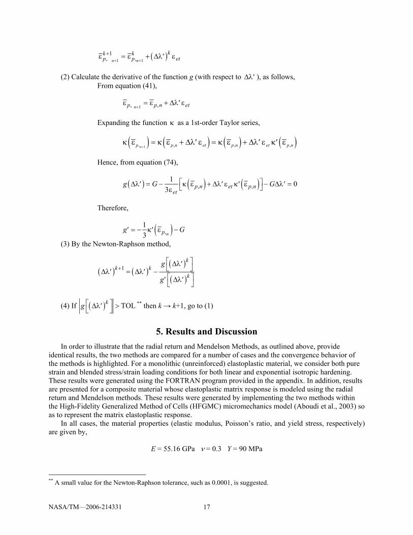
The normal stresses induced due to applied loading of the form ε11 = 0.02, ε22 = ε33 = – 0.01, ε23 = ε13 = ε12 = 0 are plotted vs. the applied ε11 in figure 1. Note that, due to the material’s isotropy, σ22 = σ33 and σ23

= σ13 = σ12 = 0. Results are shown for cases in which the loading has been applied using both 200 and 4 increments. As Fig. 1 indicates, results from the radial return and Mendelson methods are identical for both the elastic-perfectly plastic (H = 0) and linear hardening cases irrespective of the number of increments employed to apply the loading. Further, the number of increments has no effect on the results as the solution at each of the four increments matches exactly with the corresponding 200 increment solution.

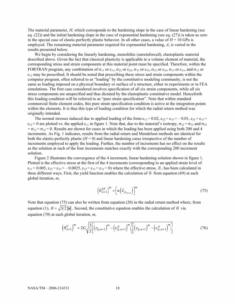
Figure 2 illustrates the convergence of the 4 increment, linear hardening solution shown in figure 1. Plotted is the effective stress at the first of the 4 increments (corresponding to an applied strain level of ε11 = 0.005, ε22 = ε33 = – 0.0025, ε23 = ε13 = ε12 = 0) where the effective stress, σ , has been calculated in three different ways. First, the yield function enables the calculation of σ from equation (69) at each global iteration, m,

( ) ( )11 , ++⎡ ⎤σ = κ ε⎣ ⎦n

mmYFn p (75)

Note that equation (75) can also be written from equation (20) in the radial return method where, from equation (1), 3 2σ = s . Second, the constitutive equation enables the calculation of σ via equation (70) at each global iteration, m,

( ) ( ) ( ) ( ) ( )1 , 1 , 1 , 1 , 1322+ + + + +⎡ ⎤ ⎡ ⎤σ = − ε − ε⎢ ⎥ ⎢ ⎥⎣ ⎦ ⎣ ⎦

m mm m mp pCn ij n n ij n nij ijG e e (76)

NASA/TM—2006-214331 19

-100

-50

0

50

100

150

200

0.000 0.005 0.010 0.015 0.020 0.025

ε11

σ11,

σ22

(MPa

)

Radial Return - 200 Inc.Radial Return - 4 Inc.Mendelson - 200 Inc.Mendelson - 4 Inc.

H = 0

H = 0

H = 10 GPa

H = 10 GPaσ22

σ11

Figure 1.—Comparison of the Radial Return and Mendelson

methods for a linearly hardening material (eq. (22)) under pure strain specification (applied strains: ε11 = 0.02, ε22 = ε33 = – 0.01, ε23 = ε13 = ε12 = 0). The induced normal stresses (σ11 and σ22 = σ33) are plotted vs. the applied ε11 for different values of the material parameter H. Note that H = 0 corresponds to the elastic-perfectly plastic case.

50

100

150

200

250

300

350

0 1 2 3Iteration Number

Effe

ctiv

e St

ress

(MPa

)

Radial ReturnMendelson

Constitutive Eqn

Yield Function

Applied Loading

Figure 2.—Comparison of the convergence behavior of the

effective stress, σ , for the Radial Return and Mendelson methods at an applied strain level of ε11 = 0.005, ε22 = ε33 = – 0.0025, ε23 = ε13 = ε12 = 0 with linear hardening and H = 10 GPa. The effective stress can be computed in three ways; from the material constitutive equation, from the yield function, and from the applied loading. All must be equal in order to ensure convergence.

Pure ε specification, linear hardening

NASA/TM—2006-214331 20

Note that, again, equation (76) can be written from equation (21) in the radial return method. Finally,

from the applied loading, the effective stress can be calculated from σ = 3 2 app appij ijs s , where app

ijs

corresponds to the stress deviator components resulting from the applied loads. In terms of strains, this can be written,

( ) ( ) ( ) ( ) ( )1 1, 1 , 1 , 1 , 11

322

− −+ + + ++

⎡ ⎤ ⎡ ⎤σ = − ε − ε⎢ ⎥ ⎢ ⎥⎣ ⎦ ⎣ ⎦

m m mm mapp p pij n n ij n nij ijn G e e (77)

where ( ) 0, 1 ,

=+ε = ε

mp pn nij ij . In the case of pure strain specification, ( )1+σ

mappn will correspond to ( ) 1

1−

+σmC

n

because the strain components, and thus the strain deviator components, ije , are specified and thus do not change from iteration to iteration. In general, however, this is not the case. When at least one stress component is specified, the strain components are redistributed as a result of accumulated plastic strain from iteration to iteration. Equation (77) is thus independent of equation (76) in the general case.

As shown in figure 2, for the case of pure strain specification with linear hardening, not only does

( )1+σmapp

n = ( ) 11

−+σ

mCn , but also ( )1+σ

mCn = ( )1+σ

mYFn = ( ) 1

1+

+σmC

n . That is, the effective stress calculated

from the constitutive equation and the yield function are identical and do not change as a function of global iteration. Therefore, for this special case (pure strain specification with linear hardening), global iteration is not necessary and the results plotted in figure 1 can be obtained with one pass through the integration algorithms presented in sections 2 and 4. Note also in figure 2 that the radial return and Mendelson methods again yield identical results.

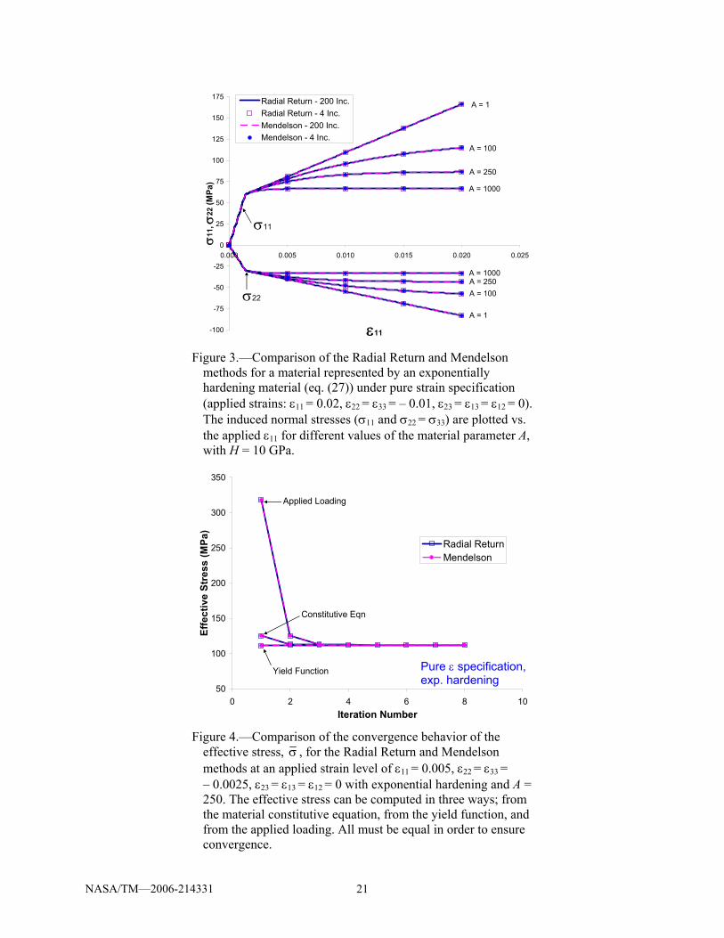
In figure 3 results compare the radial return and Mendelson methods for the monolithic elastoplastic material with exponential hardening. As in figure 1, the normal stresses induced due to applied loading of the form ε11 = 0.02, ε22 = ε33 = – 0.01, ε23 = ε13 = ε12 = 0 are plotted versus the applied ε11 for both 200 and 4 increments. The parameter H = 10 GPa and the value of the parameter A (see eq. (27)) is varied between 1 (which corresponds to nearly linear hardening) and 1000. Figure 3 illustrates that, once again, the radial return and Mendelson methods are identical and that the results are not affected by the number of increments employed to apply the loading. In addition, the effect of the parameter A on the exponential hardening results is clearly shown. Finally, note that, since all results in figure 3 employ the same value of the parameter H, their initial post yield slopes are identical.

Figure 4 shows a plot of the three effective stress values vs. global iteration number for the case of exponential hardening with A = 250 and 4 increments at the first increment. As was the case in figure 2,

figure 4 shows that ( )1+σmapp

n = ( ) 11

−+σ

mCn , which will always be the case in pure strain specification.

Now, however, the effective stress values calculated from the yield function and from the constitutive equation do not correspond until convergence has been achieved. This is because of the nonlinear function employed to describe the material’s hardening behavior. Note that convergence is rapid; 1+σC

n

and 1+σYFn are within 1 percent of each other after two iterations.

Next, consider a loading condition involving specification of both stress and strain components on the elastoplastic material. This loading condition will be referred to as “blended specification”. The loading will take the form of a specified normal strain component in one direction with a stress-free condition specified for all other components. That is, we apply, ε11 = 0.02, σ22 = σ33 = σ23 = σ13 = σ12 = 0, which

NASA/TM—2006-214331 21

-100

-75

-50

-25

0

25

50

75

100

125

150

175

0.000 0.005 0.010 0.015 0.020 0.025

ε11

σ11,

σ22

(MPa

)


A = 1000

A = 250

A = 100

A = 1

A = 1000A = 250A = 100

A = 1

σ22

σ11


methods for a material represented by an exponentially hardening material (eq. (27)) under pure strain specification (applied strains: ε11 = 0.02, ε22 = ε33 = – 0.01, ε23 = ε13 = ε12 = 0). The induced normal stresses (σ11 and σ22 = σ33) are plotted vs. the applied ε11 for different values of the material parameter A, with H = 10 GPa.

50

100

150

200

250

300

350

0 2 4 6 8 10Iteration Number

Effe

ctiv

e St

ress

(MPa

)


Constitutive Eqn

Yield Function

Applied Loading


effective stress, σ , for the Radial Return and Mendelson methods at an applied strain level of ε11 = 0.005, ε22 = ε33 = – 0.0025, ε23 = ε13 = ε12 = 0 with exponential hardening and A = 250. The effective stress can be computed in three ways; from the material constitutive equation, from the yield function, and from the applied loading. All must be equal in order to ensure convergence.

Pure ε specification, exp. hardening

NASA/TM—2006-214331 22

simulates the state experienced by the material in a standard strain controlled tensile test. Figure 5 plots the stress-strain curves in the applied strain direction (i.e., σ11 vs. ε11), along with the induced normal strain in the unapplied direction (i.e., σ11 vs. ε22 = ε33) for a linear hardening elastoplastic material where the loading has been applied using 200 and 4 increments. The radial return and Mendelson methods are compared. As in figures 1 and 3, figure 5 shows that the radial return and Mendelson methods provide identical results in both the elastic-perfectly plastic (H = 0) and linear hardening cases. The number of increments employed also has no effect on the results.

Figure 6 provides a plot of the global convergence behavior of the effective stress (again calculated in three different ways) for the first increment of the 4 increment case plotted in figure 5. As was shown in figures 2 and 4, the convergence of the radial return and Mendelson methods are again identical. Further, as was the case in figure 2, since the material hardening is linear, the effective stresses calculated from the yield function and from the constitutive equation are identical. However, due to the blended loading specification, the effective stress calculated from the applied loading is independent. This is because, in the case of blended specification, the strain deviator components change from iteration to iteration and thus equations (77) and (76) are independent. Recall that under pure strain specification, the strain deviator components are known exactly for a given load increment and do not change as a function of

iteration number. In such a case, ( )1+σmapp

n = ( ) 11

−+σ

mCn . The key point illustrated in figure 6 is that,

because the yield function and constitutive equation effective stress values are identical, but not converged, these two effective stress values cannot be used as a measure of convergence in the case of linear hardening with loading other than pure strain control. Were such a measure used, both the radial return and Mendelson methods would converge immediately to an incorrect solution that violates the specified loading condition (e.g., the stress components prescribed as zero would be non-zero).

0

50

100

150

200

250

300

-0.015 -0.010 -0.005 0.000 0.005 0.010 0.015 0.020 0.025ε11, ε22

σ11

(MPa

)


H = 0 H = 0

H = 10 GPaH = 10 GPa

ε11ε22


methods for a material represented by a linearly hardening material (eq. (22)) under blended specification (applied load: ε11 = 0.02, σ22 = σ33 = σ23 = σ13 = σ12 = 0). The normal strains (ε11 and ε22 = ε33) are plotted vs. σ11 for different values of the material parameter H. Note that H = 0 corresponds to the elastic-perfectly plastic case.

NASA/TM—2006-214331 23

50

100

150

200

250

300

0 2 4 6 8 10Iteration Number

Effe

ctiv

e St

ress

(MPa

)


Yield Function & Constitutive Eqn

Applied Loading


effective stress, σ , for the Radial Return and Mendelson methods at an applied strain level of ε11 = 0.005, σ22 = σ33 = σ23 = σ13 = σ12 = 0 with linear hardening and H = 10 GPa. The effective stress can be computed in three ways; from the material constitutive equation, from the yield function, and from the applied loading. All must be equal in order to ensure convergence.

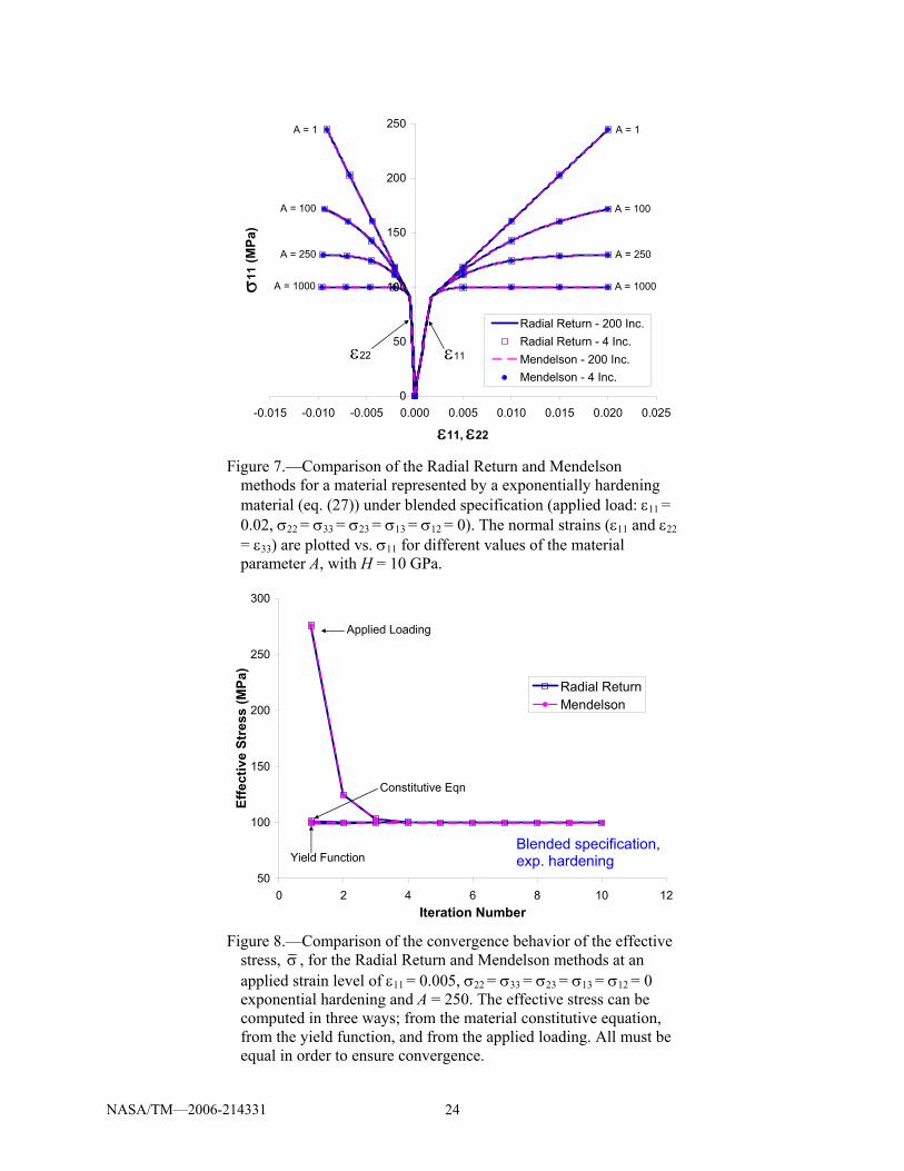
The radial return and Mendelson methods are compared in figure 7 in the case of blended specification for an exponential hardening material with a varying value of the parameter A. The specified loading is identical to that employed in figure 5, and 200 and 4 increments have again been used. As observed previously, the radial return and Mendelson methods provide identical results and the number of increments employed is of no consequence. In figure 8, the convergence behavior of the effective stress is shown for the first increment of the 4 increment case from figure 7 with A = 250. Once again, the radial return and Mendelson methods are identical. As was the case in figure 6, the effective stress calculated from the applied loading is independent of that calculated from the constitutive equation due to the blended specification (see eqs. (76) and (77)). Unlike figure 6, however, figure 8 indicates that, due to the nonlinear hardening behavior of the elastoplastic material, the effective stress calculated from the constitutive equation and the yield function are no longer coincident. Thus, in this case, these two effective stress values could be used as a measure of global convergence.

As a final illustration of the radial return and Mendelson methods, both implementations have been incorporated into a micromechanics model to enable the prediction of the response of a continuous composite material with elastoplastic phases. The High-Fidelity Generalized Method of Cells (HFGMC) micromechanics model (Aboudi et. al, 2003) has been employed for this purpose. This semi-analytical (non-FEA) model discretizes the composite repeating unit cell geometry into an arbitrary number of subcells, each of which may contain a distinct, arbitrary material. HFGMC localizes an arbitrary, admissible combination of stress and strain components on a composite material to determine the point-wise stresses and strains throughout the fiber and matrix constituents. These point-wise stress and strain components can thus be passed to a local constitutive model (such as classical plasticity) in order to simulate the local plastic response at each point. The local plastic strains are then homogenized by HFGMC to determine composite-level inelastic strains. Note that, in the linear elastic case, the HFGMC localization/homogenization method provides the effective thermo-elastic properties of the composite materials from those of the constituents.

Blended specification, linear hardening

NASA/TM—2006-214331 24

0

50

100

150

200

250

-0.015 -0.010 -0.005 0.000 0.005 0.010 0.015 0.020 0.025

ε11, ε22

σ11

(MPa

)


A = 1000

A = 250

A = 100

A = 1

A = 1000

A = 250

A = 100

A = 1

ε22 ε11


methods for a material represented by a exponentially hardening material (eq. (27)) under blended specification (applied load: ε11 = 0.02, σ22 = σ33 = σ23 = σ13 = σ12 = 0). The normal strains (ε11 and ε22

= ε33) are plotted vs. σ11 for different values of the material parameter A, with H = 10 GPa.

50

100

150

200

250

300

0 2 4 6 8 10 12Iteration Number

Effe

ctiv

e St

ress

(MPa

)


Yield Function

Applied Loading

Constitutive Eqn

Figure 8.—Comparison of the convergence behavior of the effective

stress, σ , for the Radial Return and Mendelson methods at an applied strain level of ε11 = 0.005, σ22 = σ33 = σ23 = σ13 = σ12 = 0 exponential hardening and A = 250. The effective stress can be computed in three ways; from the material constitutive equation, from the yield function, and from the applied loading. All must be equal in order to ensure convergence.

Blended specification, exp. hardening

NASA/TM—2006-214331 25

The HFGMC repeating unit cell employed herein is shown in figure 9, where the fiber and matrix constituents are depicted in different colors. As shown, in the plane of the fiber’s cross-section, the repeating unit cell is discretized into 8 by 8 subcells, whereas, in the out of plane direction, the material is considered to be infinitely long. The matrix material’s properties E, ν, and Y are taken as those of the elastoplastic material considered above. The fiber material is taken to be elastic with properties given by,

E = 413.7 GPa ν = 0.2

We consider blended stress/strain component specification on a 35 percent fiber volume fraction composite, simulating a transverse uniaxial strain controlled tensile test such that ε22 = 0.01, σ11 = σ33 = σ23 = σ13 = σ12 = 0. Results are shown in figure 10, where the composite stress-strain curves in the applied direction (i.e., σ22 vs. ε22) are plotted, along with the normal strains induced in the composite (i.e., σ22 vs. ε11 and σ22 vs. ε33). Three types of elastoplastic matrix materials are considered: elastic-perfectly plastic, linear hardening with H = 10 GPa, and exponential hardening with H = 10 GPa and A = 100. Cases involving 100 increments and 4 increments are considered, and the radial return and Mendelson methods are once again compared. First, it is clear from figure 10 that the stiff continuous fiber in the x1-direction restrains the composite in this direction, resulting in an induced ε11 that is significantly smaller than the induced ε33. Second, we see that, as in all other cases, the radial return and Mendelson methods produce identical results. Unlike previous results, however, the number of increments employed does have an effect on the predicted composite response, with the results for 4 increments slightly underpredicting the composite stress-strain curves. It was determined (but not shown) that for the present case, approximately 10 increments were required to achieve good convergence of the composite level stresses and strains.

Figure 9.—HFGMC micromechanics theory repeating unit cell employed to simulate the transverse behavior of a composite material.

NASA/TM—2006-214331 26

0

50

100

150

200

250

300

350

400

-0.010 -0.005 0.000 0.005 0.010

ε11, ε22, ε33

σ22

(MPa

)


Elastic-Perfectly Plastic Matrix

Elastic-Perfectly Plastic Matrix

Exponential Hardening Matrix (A = 100)

Exponential Hardening Matrix (A = 100)

Linear Hardening Matrix Linear

Hardening Matrix

ε11

ε22ε33


methods utilized to simulate the matrix behavior within a 35 percent volume fraction composite material under blended specification (applied load: ε22 = 0.02, σ11 = σ33 = σ23 = σ13 = σ12 = 0; transverse loading). The normal strains (ε11, ε22, and ε33) are plotted vs. σ22 for linear hardening, exponential hardening, and elastic-perfectly plastic matrix behavior.

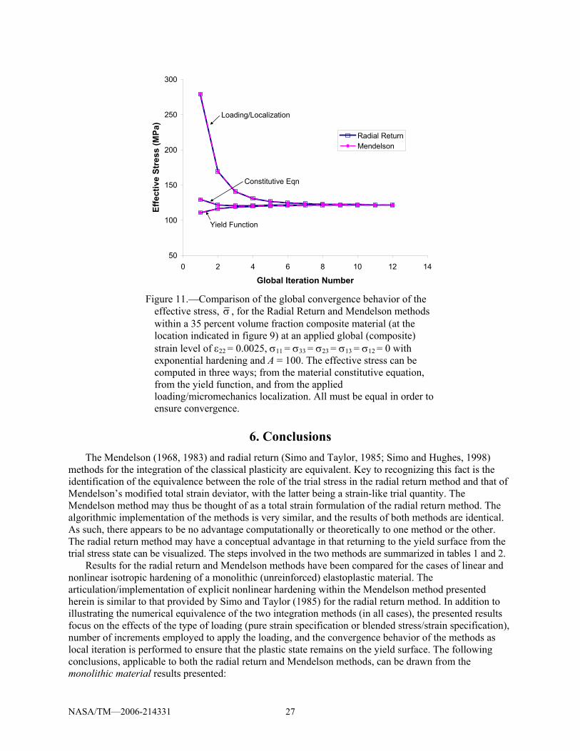
Figure 11 illustrates sample convergence behavior for the composite simulations. As in figures 2, 4, 6, and 8, figure 11 illustrates the effective stress convergence for the first increment in the case that employed 4 increments. Figure 11 is further specific to the exponential hardening case from figure 10. In addition, because the local behavior is different at each location within the composite matrix, figure 11 is applicable to one particular matrix location; that specified by the red “x” in figure 9. Figure 11 shows that the radial return and Mendelson methods again provide identical results. Further, as was the case for the monolithic (unreinforced) elastoplastic material with blended specification, the effective stress calculated from the constitutive equation and the load/localization procedure are unique. In fact, in the case of a composite, because the stresses and strains are localized from the applied composite-level stresses and strains, the local convergence will behave in this way regardless of the form of the specified composite level loading. That is, the distribution of the strain components (and thus the strain deviator components, eij) at a given point are always free to change from iteration to iteration regardless of the form of the specified loading on the composite. This is because this local strain component distribution is dictated by the micromechanics localization, which is influenced by the state at every other point in the composite, each of which is at a different point along its yield function. It is also noteworthy in figure 11 that the convergence is considerably more gradual compared to the monolithic elastoplastic material convergence illustrated in figures 2, 4, 6, and 8.

NASA/TM—2006-214331 27

50

100

150

200

250

300

0 2 4 6 8 10 12 14

Global Iteration Number

Effe

ctiv

e St

ress

(MPa

)


Loading/Localization

Yield Function

Constitutive Eqn

Figure 11.—Comparison of the global convergence behavior of the

effective stress, σ , for the Radial Return and Mendelson methods within a 35 percent volume fraction composite material (at the location indicated in figure 9) at an applied global (composite) strain level of ε22 = 0.0025, σ11 = σ33 = σ23 = σ13 = σ12 = 0 with exponential hardening and A = 100. The effective stress can be computed in three ways; from the material constitutive equation, from the yield function, and from the applied loading/micromechanics localization. All must be equal in order to ensure convergence.

6. Conclusions The Mendelson (1968, 1983) and radial return (Simo and Taylor, 1985; Simo and Hughes, 1998)

methods for the integration of the classical plasticity are equivalent. Key to recognizing this fact is the identification of the equivalence between the role of the trial stress in the radial return method and that of Mendelson’s modified total strain deviator, with the latter being a strain-like trial quantity. The Mendelson method may thus be thought of as a total strain formulation of the radial return method. The algorithmic implementation of the methods is very similar, and the results of both methods are identical. As such, there appears to be no advantage computationally or theoretically to one method or the other. The radial return method may have a conceptual advantage in that returning to the yield surface from the trial stress state can be visualized. The steps involved in the two methods are summarized in tables 1 and 2.

Results for the radial return and Mendelson methods have been compared for the cases of linear and nonlinear isotropic hardening of a monolithic (unreinforced) elastoplastic material. The articulation/implementation of explicit nonlinear hardening within the Mendelson method presented herein is similar to that provided by Simo and Taylor (1985) for the radial return method. In addition to illustrating the numerical equivalence of the two integration methods (in all cases), the presented results focus on the effects of the type of loading (pure strain specification or blended stress/strain specification), number of increments employed to apply the loading, and the convergence behavior of the methods as local iteration is performed to ensure that the plastic state remains on the yield surface. The following conclusions, applicable to both the radial return and Mendelson methods, can be drawn from the monolithic material results presented:

NASA/TM—2006-214331 28

(1) The results are independent of the number of increments used to apply the load. (2) Local iteration is not necessary in the case of pure strain specification with linear isotropic

hardening.

(3) Local iteration is necessary in the cases of blended specification or nonlinear isotropic hardening. (4) Blended specification with linear isotropic hardening represents a special case in that the effective

stress value calculated from the constitutive equation and the yield function are identical for a given iteration, though not necessarily converged. These two values thus cannot be used as a convergence criterion in this case. In this case, the effective stress value calculated from the applied loading may be compared with one of the other two effective stress values to gauge convergence. However, employing this applied loading effective stress value in all cases to determine convergence may result in the performance of an extra, unnecessary iteration.

(5) Pure strain specification behaves differently than blended specification because the distribution

(i.e., proportion) of the strain components is prescribed and thus known a priori. The plasticity equations then need only separate each strain component into elastic and inelastic parts. In contrast, under blended specification, the plasticity equations can find a strain component distribution corresponding to a plastic state that is on the yield surface, but does not satisfy the specified blended loading.

Results for a composite material whose elastoplastic matrix material was modeled using the radial

return and Mendelson classical plasticity methods were also presented. The composite analysis employed the non-FEA High-Fidelity Generalized Method of Cells (HFGMC) micromechanics model (Aboudi et al., 2003) developed by the authors. Results using both integration methods were once again identical, however, in contrast to the monolithic material results, the number of increments employed to apply the loading now had an effect. Finally, because the local stresses and strains have been localized from the applied composite-level stresses and strains, the convergence behavior is similar to that of the monolithic case with blended specification and nonlinear hardening. Iteration is required regardless of the nature of the loading applied on the composite and the type of hardening. This fact is somewhat intuitive because the in situ stresses within the micromechanics representation of the composite are multi-axial and progress in a non-proportional way irrespective of the nature of the global composite-level loading. Thus, on the local level, the micromechanics problem is similar to the blended specification monolithic material case where the correct proportional distribution of the strain components is not known a priori.

References 1. Aboudi, J., Pindera, M.-J., and Arnold, S.M. (2003) “Higher-Order Theory for Periodic Multiphase

Materials with Inelastic Phases” International Journal of Plasticity 19, 805–847. 2. Mendelson, A. (1968) Plasticity: Theory and Application, MacMillan, New York. 3. Mendelson, A. (1983) Plasticity: Theory and Application, Reprint Edition, Krieger, Malabar, FL. 4. Simo, J.C. and Taylor, R.L. (1985) “Consistent Tangent Operators for Rate-Independent

Elastoplasticity” Computer Methods in Applied Mechanics and Engineering 48, 101–118. 5. Simo, J.C. and Hughes, T.J.R. (1998) Computational Inelasticity, Springer, New York. 6. Wilkins, M. L. (1964) Calculation of elastic-plastic flow. In Alder, B., Fernbach, S., and Rotenberg,

M., editors, Methods in Computational Physics V.3, pages 211–263. Academic Press, New York, 1964.

NASA/TM—2006-214331 29

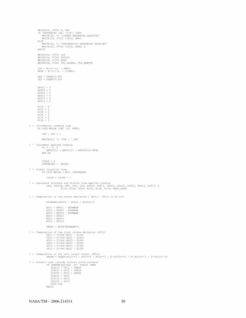
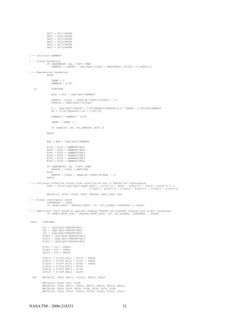
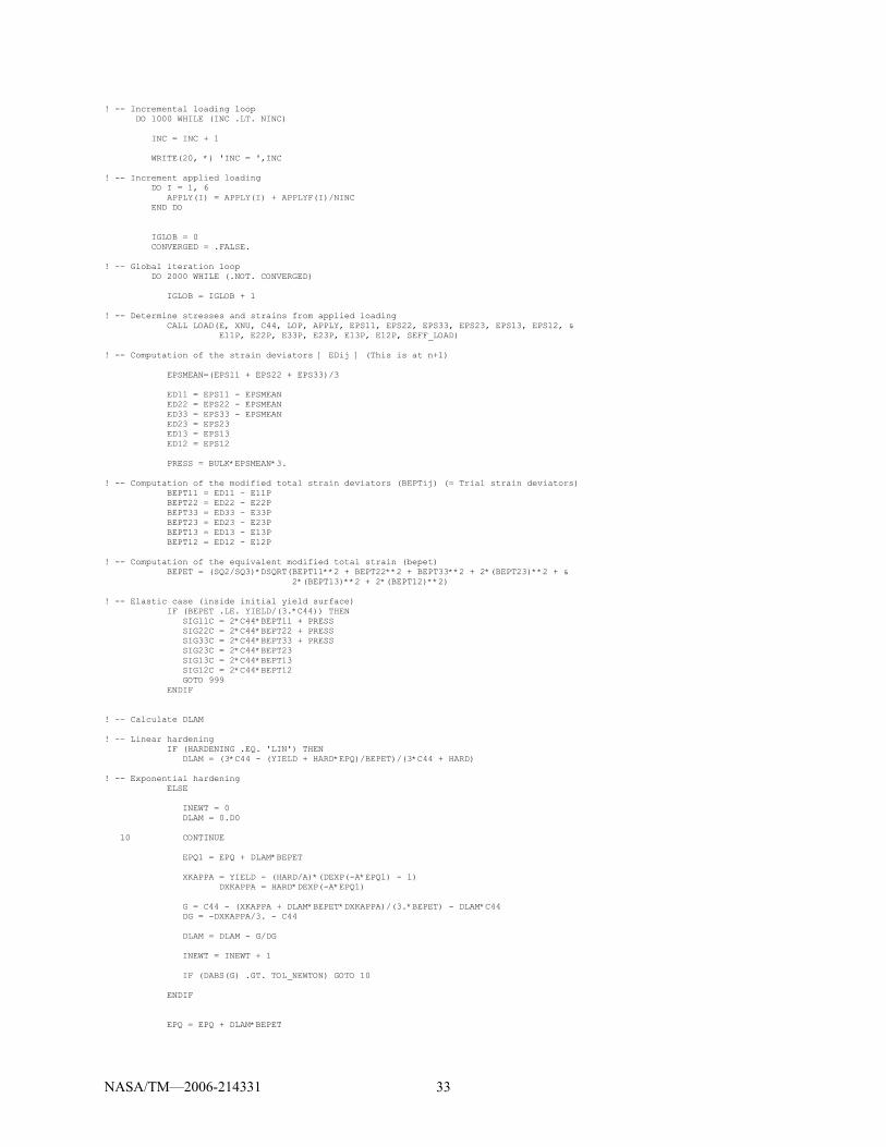
Appendix

Radial Return and Mendelson Methods FORTRAN Program

!********************************************************************************************************************** !********************************************************************************************************************** PROGRAM MAIN !---------------------------------------------------------------------------------------------------------------------- ! -- Integrates the classical plasticity equations for arbitrary monotonic loading using the Radial Return and ! Mendelson methods for linear and exponential isotropic hardening materials !---------------------------------------------------------------------------------------------------------------------- IMPLICIT DOUBLE PRECISION (A-H,O-Z) CHARACTER*3 :: HARDENING INTEGER :: LOP(6) DOUBLE PRECISION :: APPLYF(6) !---------------------------------------------------------------------------------------------------------------------- ! -- Properties E = 55160. XNU = 0.3 YIELD = 90. HARD = 10000. ! HARD = 0. A = 1000. ! A = 0.0000001 ! -- 6 Components of applied loading ! -- LOP = 1 ---> strain; LOP = 2 ---> stress LOP(1) = 1 LOP(2) = 2 LOP(3) = 2 LOP(4) = 2 LOP(5) = 2 LOP(6) = 2 APPLYF(1) = 0.02 APPLYF(2) = 0. APPLYF(3) = 0. APPLYF(4) = 0. APPLYF(5) = 0. APPLYF(6) = 0. ! -- Number of increments NINC = 4 ! HARDENING = 'LIN' HARDENING = 'NON' TOL_GLOBAL = 0.0000001 TOL_NEWTON = 0.0001 CALL RADIAL_RETURN(E, XNU, YIELD, HARD, A, LOP, APPLYF, TOL_GLOBAL, TOL_NEWTON, NINC, HARDENING) CALL MENDELSON(E, XNU, YIELD, HARD, A, LOP, APPLYF, TOL_GLOBAL, TOL_NEWTON, NINC, HARDENING) END !********************************************************************************************************************** !********************************************************************************************************************** SUBROUTINE RADIAL_RETURN(E, XNU, YIELD, HARD, A, LOP, APPLYF, TOL_GLOBAL, TOL_NEWTON, NINC, HARDENING) !---------------------------------------------------------------------------------------------------------------------- ! -- Integrates the classical plasticity equations for arbitrary monotonic loading ! using the Radial Return method !---------------------------------------------------------------------------------------------------------------------- IMPLICIT DOUBLE PRECISION (A-H,O-Z) CHARACTER*3 :: HARDENING LOGICAL :: CONVERGED INTEGER :: LOP(6) DOUBLE PRECISION :: APPLYF(6), APPLY(6) !---------------------------------------------------------------------------------------------------------------------- OPEN(22, FILE='radial_return.plot', STATUS='UNKNOWN') OPEN(23, FILE='radial_return.conv', STATUS='UNKNOWN') OPEN(24, FILE='radial_return.out', STATUS='UNKNOWN') WRITE(24, *) 'RADIAL RETURN METHOD OUTPUT' WRITE(24, *) '---------------------------'

NASA/TM—2006-214331 30

WRITE(24, 9700) E, XNU IF (HARDENING .EQ. 'LIN') THEN WRITE(24, *) 'LINEAR HARDENING SELECTED' WRITE(24, 9710) YIELD, HARD ELSE WRITE(24, *) 'EXPONENTIAL HARDENING SELECTED' WRITE(24, 9720) YIELD, HARD, A ENDIF WRITE(24, 9725) LOP WRITE(24, 9730) APPLYF WRITE(24, 9735) NINC WRITE(24, 9740) TOL_GLOBAL, TOL_NEWTON C44 = E/(2.*(1. + XNU)) BULK = E/(3.*(1. - 2*XNU)) SQ2 = DSQRT(2.D0) SQ3 = DSQRT(3.D0) EPS11 = 0 EPS22 = 0 EPS33 = 0 EPS23 = 0 EPS13 = 0 EPS12 = 0 E11P = 0 E22P = 0 E33P = 0 E23P = 0 E13P = 0 E12P = 0 ! -- Incremental loading loop DO 1000 WHILE (INC .LT. NINC) INC = INC + 1 WRITE(23, *) 'INC = ',INC ! -- Increment applied loading DO I = 1, 6 APPLY(I) = APPLY(I) + APPLYF(I)/NINC END DO IGLOB = 0 CONVERGED = .FALSE. ! -- Global iteration loop DO 2000 WHILE (.NOT. CONVERGED) IGLOB = IGLOB + 1 ! -- Determine stresses and strains from applied loading CALL LOAD(E, XNU, C44, LOP, APPLY, EPS11, EPS22, EPS33, EPS23, EPS13, EPS12, & E11P, E22P, E33P, E23P, E13P, E12P, SEFF_LOAD) ! -- Computation of the strain deviators [ EDij ] (This is at n+1) EPSMEAN=(EPS11 + EPS22 + EPS33)/3 ED11 = EPS11 - EPSMEAN ED22 = EPS22 - EPSMEAN ED33 = EPS33 - EPSMEAN ED23 = EPS23 ED13 = EPS13 ED12 = EPS12 PRESS = BULK*EPSMEAN*3. ! -- Computation of the trial stress deviators (STij) ST11 = 2*C44*(ED11 - E11P) ST22 = 2*C44*(ED22 - E22P) ST33 = 2*C44*(ED33 - E33P) ST23 = 2*C44*(ED23 - E23P) ST13 = 2*C44*(ED13 - E13P) ST12 = 2*C44*(ED12 - E12P) ! -- Computation of the unit normal vector (XNij) XNORM = DSQRT(ST11**2 + ST22**2 + ST33**2 + 2*(ST23)**2 + 2*(ST13)**2 + 2*(ST12)**2) ! -- Elastic case (inside initial yield surface) IF (XNORM*SQ3/SQ2 .LT. YIELD) THEN SIG11C = ST11 + PRESS SIG22C = ST22 + PRESS SIG33C = ST33 + PRESS SIG23C = ST23 SIG13C = ST13 SIG12C = ST12 GOTO 999 ENDIF

NASA/TM—2006-214331 31

XN11 = ST11/XNORM XN22 = ST22/XNORM XN33 = ST33/XNORM XN23 = ST23/XNORM XN13 = ST13/XNORM XN12 = ST12/XNORM ! -- Calculate GAMMADT ! -- Linear hardening IF (HARDENING .EQ. 'LIN') THEN GAMMADT = (XNORM - (SQ2/SQ3)*(YIELD + HARD*EPQ))/(2*C44 + 2.*HARD/3.) ! -- Exponential hardening ELSE INEWT = 0 GAMMADT = 0.D0 10 CONTINUE EPQ1 = EPQ + (SQ2/SQ3)*GAMMADT XKAPPA = YIELD - (HARD/A)*(DEXP(-A*EPQ1) - 1) DXKAPPA = HARD*DEXP(-A*EPQ1) G = -(SQ2/SQ3)*XKAPPA - 2.D0*GAMMADT*DXKAPPA/3.0 + XNORM - 2.D0*C44*GAMMADT DG = -2.D0*DXKAPPA/3.D0 - 2.D0*C44 GAMMADT = GAMMADT - G/DG INEWT = INEWT + 1 IF (DABS(G) .GT. TOL_NEWTON) GOTO 10 ENDIF EPQ = EPQ + (SQ2/SQ3)*GAMMADT E11P = E11P + GAMMADT*XN11 E22P = E22P + GAMMADT*XN22 E33P = E33P + GAMMADT*XN33 E23P = E23P + GAMMADT*XN23 E13P = E13P + GAMMADT*XN13 E12P = E12P + GAMMADT*XN12 IF (HARDENING .EQ. 'LIN') THEN XKAPPA = YIELD + HARD*EPQ ELSE XKAPPA = YIELD - (HARD/A)*(DEXP(-A*EPQ) - 1) ENDIF ! -- Calculate effective stress from constitutive eqn (= XKAPPA for convergence) SEFF = 2*C44*(SQ3/SQ2)*DSQRT((ED11 - E11P)**2 + (ED22 - E22P)**2 + (ED33 - E33P)**2 + & 2*(ED23 - E23P)**2 + 2*(ED13 - E13P)**2 + 2*(ED12 - E12P)**2) WRITE(23, 9100) IGLOB, SEFF, XKAPPA, SEFF_LOAD, EPQ ! -- Global convergence check CONVERGED = .TRUE. IF (DABS((SEFF - XKAPPA)/SEFF) .GT. TOL_GLOBAL) CONVERGED = .FALSE. ! -- Additional check based on applied loading (needed for blended loading with linear hardening) IF (DABS((SEFF_LOAD - XKAPPA)/SEFF_LOAD) .GT. TOL_GLOBAL) CONVERGED = .FALSE. 2000 CONTINUE S11 = (SQ2/SQ3)*XKAPPA*XN11 S22 = (SQ2/SQ3)*XKAPPA*XN22 S33 = (SQ2/SQ3)*XKAPPA*XN33 SIG23 = (SQ2/SQ3)*XKAPPA*XN23 SIG13 = (SQ2/SQ3)*XKAPPA*XN13 SIG12 = (SQ2/SQ3)*XKAPPA*XN12 SIG11 = S11 + PRESS SIG22 = S22 + PRESS SIG33 = S33 + PRESS SIG11C = 2*C44*(ED11 - E11P) + PRESS SIG22C = 2*C44*(ED22 - E22P) + PRESS SIG33C = 2*C44*(ED33 - E33P) + PRESS SIG23C = 2*C44*(ED23 - E23P) SIG13C = 2*C44*(ED13 - E13P) SIG12C = 2*C44*(ED12 - E12P) 999 WRITE(22, 9000) EPS11, SIG11C, EPS22, EPS33 WRITE(24, 9200) INC, IGLOB WRITE(24, 9300) EPS11, EPS22, EPS33, EPS23, EPS13, EPS12 WRITE(24, 9400) E11P, E22P, E33P, E23P, E13P, E12P WRITE(24, 9500) SIG11, SIG22, SIG33, SIG23, SIG13, SIG12

NASA/TM—2006-214331 32

WRITE(24, 9600) SIG11C, SIG22C, SIG33C, SIG23C, SIG13C, SIG12C 1000 CONTINUE CLOSE(22) CLOSE(23) CLOSE(24) RETURN !---------------------------------------------------------------------------------------------------------------------- 9000 FORMAT(4(E12.5,2X)) 9100 FORMAT(I3,2X,4(E12.5,2X)) 9200 FORMAT(//,'INCREMENT # ', I4, 6X,' # GLOBAL ITERATIONS ',I4) 9300 FORMAT(' TOTAL STRAIN COMPONENTS:',/,3X,6(E12.5,1X)) 9400 FORMAT(' PLASTIC STRAIN COMPONENTS:',/,3X,6(E12.5,1X)) 9500 FORMAT(' STRESS COMPONENTS FROM YIELD FUNCTION:',/,3X,6(E12.5,1X)) 9600 FORMAT(' STRESS COMPONENTS FROM CONSTITUTIVE EQN:',/,3X,6(E12.5,1X)) 9700 FORMAT(//,' ELASTIC MATERIAL PARAMETERS:',/,3X,'ELASTIC MODULUS ',E12.5,/,3X,'POISSON RATIO ',F7.5,/) 9710 FORMAT(/,' PLASTIC MATERIAL PARAMETERS:',/,3X,'YIELD STRESS ',E12.5,/,3X,'HARDENING SLOPE ',E12.5) 9720 FORMAT(/,' PLASTIC MATERIAL PARAMETERS:',/,3X,'YIELD STRESS ',E12.5,/,3X,'HARDENING SLOPE ',E12.5,/,3X, & 'EXP. PARAMETER A ',E12.5) 9725 FORMAT(/,' APPLIED LOAD (1 = STRAIN; 2 = STRESS):',/,6(I12,1X)) 9730 FORMAT(5X,6(E12.5,1X)) 9735 FORMAT(/,' NUMBER OF INCREMENTS ',I4) 9740 FORMAT(/,' TOLERANCE FOR GLOBAL ITERATIONS: ',E12.5,/,' TOLERANCE FOR NEWTON-RAPHSON ITERATIONS: ',E12.5) END !********************************************************************************************************************** !********************************************************************************************************************** SUBROUTINE MENDELSON(E, XNU, YIELD, HARD, A, LOP, APPLYF, TOL_GLOBAL, TOL_NEWTON, NINC, HARDENING) !---------------------------------------------------------------------------------------------------------------------- ! -- Integrates the classical plasticity equations for arbitrary monotonic loading ! using the Mendelson method !---------------------------------------------------------------------------------------------------------------------- IMPLICIT DOUBLE PRECISION (A-H,O-Z) CHARACTER*3 :: HARDENING LOGICAL :: CONVERGED INTEGER :: LOP(6) DOUBLE PRECISION :: APPLYF(6), APPLY(6) !---------------------------------------------------------------------------------------------------------------------- OPEN(19, FILE='mendelson.plot', STATUS='UNKNOWN') OPEN(20, FILE='mendelson.conv', STATUS='UNKNOWN') OPEN(21, FILE='mendelson.out', STATUS='UNKNOWN') WRITE(21, *) 'MENDELSON METHOD OUTPUT' WRITE(21, *) '-----------------------' WRITE(21, 9700) E, XNU IF (HARDENING .EQ. 'LIN') THEN WRITE(21, *) 'LINEAR HARDENING SELECTED' WRITE(21, 9710) YIELD, HARD ELSE WRITE(21, *) 'EXPONENTIAL HARDENING SELECTED' WRITE(21, 9720) YIELD, HARD, A ENDIF WRITE(21, 9725) LOP WRITE(21, 9730) APPLYF WRITE(21, 9735) NINC WRITE(21, 9740) TOL_GLOBAL, TOL_NEWTON C44 = E/(2.*(1. + XNU)) BULK = E/(3.*(1. - 2*XNU)) SQ2 = DSQRT(2.D0) SQ3 = DSQRT(3.D0) EPS11 = 0 EPS22 = 0 EPS33 = 0 EPS23 = 0 EPS13 = 0 EPS12 = 0 E11P = 0 E22P = 0 E33P = 0 E23P = 0 E13P = 0 E12P = 0

NASA/TM—2006-214331 33

! -- Incremental loading loop DO 1000 WHILE (INC .LT. NINC) INC = INC + 1 WRITE(20, *) 'INC = ',INC ! -- Increment applied loading DO I = 1, 6 APPLY(I) = APPLY(I) + APPLYF(I)/NINC END DO IGLOB = 0 CONVERGED = .FALSE. ! -- Global iteration loop DO 2000 WHILE (.NOT. CONVERGED) IGLOB = IGLOB + 1 ! -- Determine stresses and strains from applied loading CALL LOAD(E, XNU, C44, LOP, APPLY, EPS11, EPS22, EPS33, EPS23, EPS13, EPS12, & E11P, E22P, E33P, E23P, E13P, E12P, SEFF_LOAD) ! -- Computation of the strain deviators [ EDij ] (This is at n+1) EPSMEAN=(EPS11 + EPS22 + EPS33)/3 ED11 = EPS11 - EPSMEAN ED22 = EPS22 - EPSMEAN ED33 = EPS33 - EPSMEAN ED23 = EPS23 ED13 = EPS13 ED12 = EPS12 PRESS = BULK*EPSMEAN*3. ! -- Computation of the modified total strain deviators (BEPTij) (= Trial strain deviators) BEPT11 = ED11 - E11P BEPT22 = ED22 - E22P BEPT33 = ED33 - E33P BEPT23 = ED23 - E23P BEPT13 = ED13 - E13P BEPT12 = ED12 - E12P ! -- Computation of the equivalent modified total strain (bepet) BEPET = (SQ2/SQ3)*DSQRT(BEPT11**2 + BEPT22**2 + BEPT33**2 + 2*(BEPT23)**2 + & 2*(BEPT13)**2 + 2*(BEPT12)**2) ! -- Elastic case (inside initial yield surface) IF (BEPET .LE. YIELD/(3.*C44)) THEN SIG11C = 2*C44*BEPT11 + PRESS SIG22C = 2*C44*BEPT22 + PRESS SIG33C = 2*C44*BEPT33 + PRESS SIG23C = 2*C44*BEPT23 SIG13C = 2*C44*BEPT13 SIG12C = 2*C44*BEPT12 GOTO 999 ENDIF ! -- Calculate DLAM ! -- Linear hardening IF (HARDENING .EQ. 'LIN') THEN DLAM = (3*C44 - (YIELD + HARD*EPQ)/BEPET)/(3*C44 + HARD) ! -- Exponential hardening ELSE INEWT = 0 DLAM = 0.D0 10 CONTINUE EPQ1 = EPQ + DLAM*BEPET XKAPPA = YIELD - (HARD/A)*(DEXP(-A*EPQ1) - 1) DXKAPPA = HARD*DEXP(-A*EPQ1) G = C44 - (XKAPPA + DLAM*BEPET*DXKAPPA)/(3.*BEPET) - DLAM*C44 DG = -DXKAPPA/3. - C44 DLAM = DLAM - G/DG INEWT = INEWT + 1 IF (DABS(G) .GT. TOL_NEWTON) GOTO 10 ENDIF EPQ = EPQ + DLAM*BEPET

NASA/TM—2006-214331 34

E11P = E11P + DLAM*BEPT11 E22P = E22P + DLAM*BEPT22 E33P = E33P + DLAM*BEPT33 E23P = E23P + DLAM*BEPT23 E13P = E13P + DLAM*BEPT13 E12P = E12P + DLAM*BEPT12 IF (HARDENING .EQ. 'LIN') THEN XKAPPA = YIELD + HARD*EPQ ELSE XKAPPA = YIELD - (HARD/A)*(DEXP(-A*EPQ) - 1) ENDIF ! -- Calculate effective stress from constitutive eqn (= XKAPPA for convergence) SEFF = 2*C44*(SQ3/SQ2)*DSQRT((ED11 - E11P)**2 + (ED22 - E22P)**2 + (ED33 - E33P)**2 + & 2*(ED23 - E23P)**2 + 2*(ED13 - E13P)**2 + 2*(ED12 - E12P)**2) WRITE(20, 9100) IGLOB, SEFF, XKAPPA, SEFF_LOAD, EPQ ! -- Global convergence check CONVERGED = .TRUE. IF (DABS((SEFF - XKAPPA)/SEFF) .GT. TOL_GLOBAL) CONVERGED = .FALSE. ! -- Additional check based on applied loading (needed for blended loading with linear hardening) IF (DABS((SEFF_LOAD - XKAPPA)/SEFF_LOAD) .GT. TOL_GLOBAL) CONVERGED = .FALSE. 2000 CONTINUE SIG11 = 2*XKAPPA*BEPT11/(3.*BEPET) + PRESS SIG22 = 2*XKAPPA*BEPT22/(3.*BEPET) + PRESS SIG33 = 2*XKAPPA*BEPT33/(3.*BEPET) + PRESS SIG23 = 2*XKAPPA*BEPT23/(3.*BEPET) SIG13 = 2*XKAPPA*BEPT13/(3.*BEPET) SIG12 = 2*XKAPPA*BEPT12/(3.*BEPET) SIG11C = 2*C44*(ED11 - E11P) + PRESS SIG22C = 2*C44*(ED22 - E22P) + PRESS SIG33C = 2*C44*(ED33 - E33P) + PRESS SIG23C = 2*C44*(ED23 - E23P) SIG13C = 2*C44*(ED13 - E13P) SIG12C = 2*C44*(ED12 - E12P) 999 WRITE(19, 9000) EPS11, SIG11C, EPS22, EPS33 WRITE(21, 9200) INC, IGLOB WRITE(21, 9300) EPS11, EPS22, EPS33, EPS23, EPS13, EPS12 WRITE(21, 9400) E11P, E22P, E33P, E23P, E13P, E12P WRITE(21, 9500) SIG11, SIG22, SIG33, SIG23, SIG13, SIG12 WRITE(21, 9600) SIG11C, SIG22C, SIG33C, SIG23C, SIG13C, SIG12C 1000 CONTINUE CLOSE(19) CLOSE(20) CLOSE(21) RETURN !---------------------------------------------------------------------------------------------------------------------- 9000 FORMAT(4(E12.5,2X)) 9100 FORMAT(I3,2X,4(E12.5,2X)) 9200 FORMAT(//,'INCREMENT # ', I4, 6X,' # GLOBAL ITERATIONS ',I4) 9300 FORMAT(' TOTAL STRAIN COMPONENTS:',/,3X,6(E12.5,1X)) 9400 FORMAT(' PLASTIC STRAIN COMPONENTS:',/,3X,6(E12.5,1X)) 9500 FORMAT(' STRESS COMPONENTS FROM YIELD FUNCTION:',/,3X,6(E12.5,1X)) 9600 FORMAT(' STRESS COMPONENTS FROM CONSTITUTIVE EQN:',/,3X,6(E12.5,1X)) 9700 FORMAT(//,' ELASTIC MATERIAL PARAMETERS:',/,3X,'ELASTIC MODULUS ',E12.5,/,3X,'POISSON RATIO ',F7.5,/) 9710 FORMAT(/,' PLASTIC MATERIAL PARAMETERS:',/,3X,'YIELD STRESS ',E12.5,/,3X,'HARDENING SLOPE ',E12.5) 9720 FORMAT(/,' PLASTIC MATERIAL PARAMETERS:',/,3X,'YIELD STRESS ',E12.5,/,3X,'HARDENING SLOPE ',E12.5,/,3X, & 'EXP. PARAMETER A ',E12.5) 9725 FORMAT(/,' APPLIED LOAD (1 = STRAIN; 2 = STRESS):',/,6(I12,1X)) 9730 FORMAT(5X,6(E12.5,1X)) 9735 FORMAT(/,' NUMBER OF INCREMENTS ',I4) 9740 FORMAT(/,' TOLERANCE FOR GLOBAL ITERATIONS: ',E12.5,/,' TOLERANCE FOR NEWTON-RAPHSON ITERATIONS: ',E12.5) END !********************************************************************************************************************** !********************************************************************************************************************** SUBROUTINE LOAD(E, XNU, C44, LOP, APPLY, EPS11, EPS22, EPS33, EPS23, EPS13, EPS12, & E11P, E22P, E33P, E23P, E13P, E12P, SEFF_LOAD) !---------------------------------------------------------------------------------------------------------------------- ! -- Given some combination of known S and E, solves for unknown components from S = C*(E - EP) !---------------------------------------------------------------------------------------------------------------------- IMPLICIT DOUBLE PRECISION (A-H,O-Z) INTEGER :: LOP(6) DOUBLE PRECISION :: APPLY(6), APPLY_E(6), C(3, 3), CN(3, 3), UN(3)

NASA/TM—2006-214331 35

!---------------------------------------------------------------------------------------------------------------------- ! -- Determine 3x3 normal component stiffness matrix C(1, 1) = E*(1 - XNU)/(1 - XNU - 2*XNU**2) C(1, 2) = E*XNU/(1 - XNU - 2*XNU**2) C(1, 3) = C(1, 2) C(2, 1) = C(1, 2) C(2, 2) = C(1, 1) C(2, 3) = C(1, 2) C(3, 1) = C(1, 2) C(3, 2) = C(1, 2) C(3, 3) = C(1, 1) ! -- Rearrange equations such that all unknowns are on r.h.s. DO 230 I = 1, 3 IF (LOP(I) .EQ. 2) THEN DO J = 1, 3 IF (J .NE. I) CN(I, J) = - C(I, J) / C(I, I) END DO CN(I, I) = 1.0 / C(I, I) ! -- Cycle through other rows DO 210 K = 1, 3 IF (K .NE. I) THEN DO J = 1, 3 IF (J .EQ. I) THEN CN(K, J) = C(K, J) / C(I, I) ELSE CN(K, J) = C(K, J) - C(K, I) * C(I, J) / C(I, I) ENDIF END DO ENDIF 210 CONTINUE ! -- Reset C for next time (i.e. next specified S) DO II = 1, 3 DO JJ = 1, 3 C(II, JJ) = CN(II, JJ) END DO END DO ENDIF 230 CONTINUE APPLY_E = APPLY IF (LOP(1) .EQ. 1) APPLY_E(1) = APPLY(1) - E11P IF (LOP(2) .EQ. 1) APPLY_E(2) = APPLY(2) - E22P IF (LOP(3) .EQ. 1) APPLY_E(3) = APPLY(3) - E33P ! -- Solve for unknowns DO I = 1, 3 UN(I) = 0 DO J = 1, 3 UN(I) = UN(I) + C(I, J)*APPLY_E(J) END DO END DO IF (LOP(1) .EQ. 1) THEN EPS11 = APPLY(1) SIG11 = UN(1) ELSE EPS11 = UN(1) + E11P SIG11 = APPLY(1) ENDIF IF (LOP(2) .EQ. 1) THEN EPS22 = APPLY(2) SIG22 = UN(2) ELSE EPS22 = UN(2) + E22P SIG22 = APPLY(2) ENDIF IF (LOP(3) .EQ. 1) THEN EPS33 = APPLY(3) SIG33 = UN(3) ELSE EPS33 = UN(3) + E33P SIG33 = APPLY(3) ENDIF IF (LOP(4) .EQ. 1) THEN EPS23 = APPLY(4) SIG23 = 2*C44*APPLY_E(4) ELSE EPS23 = APPLY_E(4)/(2*C44) + E23P SIG23 = APPLY(4) ENDIF

NASA/TM—2006-214331 36

IF (LOP(5) .EQ. 1) THEN EPS13 = APPLY(5) SIG13 = 2*C44*APPLY_E(5) ELSE EPS13 = APPLY_E(5)/(2*C44) + E13P SIG13 = APPLY(5) ENDIF IF (LOP(6) .EQ. 1) THEN EPS12 = APPLY(6) SIG12 = 2*C44*APPLY_E(6) ELSE EPS12 = APPLY_E(6)/(2*C44) + E12P SIG12 = APPLY(6) ENDIF ! -- Determine effective stress according to applied load SEFF_LOAD = DSQRT((SIG11 - SIG22)**2 + (SIG22 - SIG33)**2 + (SIG11 - SIG33)**2 + & 6.*(SIG23**2 + SIG13**2 + SIG12**2)) / DSQRT(2.D0) RETURN END !********************************************************************************************************************** !**********************************************************************************************************************

This publication is available from the NASA Center for AeroSpace Information, 301–621–0390.

REPORT DOCUMENTATION PAGE

2. REPORT DATE

19. SECURITY CLASSIFICATION OF ABSTRACT

18. SECURITY CLASSIFICATION OF THIS PAGE

Public reporting burden for this collection of information is estimated to average 1 hour per response, including the time for reviewing instructions, searching existing data sources,gathering and maintaining the data needed, and completing and reviewing the collection of information. Send comments regarding this burden estimate or any other aspect of thiscollection of information, including suggestions for reducing this burden, to Washington Headquarters Services, Directorate for Information Operations and Reports, 1215 JeffersonDavis Highway, Suite 1204, Arlington, VA 22202-4302, and to the Office of Management and Budget, Paperwork Reduction Project (0704-0188), Washington, DC 20503.

NSN 7540-01-280-5500 Standard Form 298 (Rev. 2-89)Prescribed by ANSI Std. Z39-18298-102

Form Approved

OMB No. 0704-0188

12b. DISTRIBUTION CODE

8. PERFORMING ORGANIZATION REPORT NUMBER

5. FUNDING NUMBERS

3. REPORT TYPE AND DATES COVERED

4. TITLE AND SUBTITLE

6. AUTHOR(S)

7. PERFORMING ORGANIZATION NAME(S) AND ADDRESS(ES)

11. SUPPLEMENTARY NOTES

12a. DISTRIBUTION/AVAILABILITY STATEMENT

13. ABSTRACT (Maximum 200 words)

14. SUBJECT TERMS

17. SECURITY CLASSIFICATION OF REPORT

16. PRICE CODE

15. NUMBER OF PAGES

20. LIMITATION OF ABSTRACT

Unclassified Unclassified

Technical Memorandum

Unclassified

National Aeronautics and Space AdministrationJohn H. Glenn Research Center at Lewis FieldCleveland, Ohio 44135–3191

1. AGENCY USE ONLY (Leave blank)

10. SPONSORING/MONITORING AGENCY REPORT NUMBER

9. SPONSORING/MONITORING AGENCY NAME(S) AND ADDRESS(ES)

National Aeronautics and Space AdministrationWashington, DC 20546–0001

Available electronically at http://gltrs.grc.nasa.gov

July 2006

NASA TM—2006-214331

E–15564

WBS 561581.02.08.03.04.05

42

The Equivalence of the Radial Return and Mendelson Methods for Integrating theClassical Plasticity Equations

Brett A. Bednarcyk, Jacob Aboudi, and Steven M. Arnold

Elastoplasticity; Algorithms; iterative solution; FORTRAN; Applications programs(computer); Deformation; Stress-strain relationships; Nonlinearity; Micromechanics;Composite materials; Mathematical models

Unclassified -UnlimitedSubject Category: 39

The radial return and Mendelson methods for integrating the equations of classical plasticity, which appear independentlyin the literature, are shown to be identical. Both methods are presented in detail as are the specifics of their algorithmicimplementation. Results illustrate the methods' equivalence across a range of conditions and address the question of whenthe methods require iteration in order for the plastic state to remain on the yield surface. FORTRAN code implementationsof the radial return and Mendelson methods are provided in the appendix.

Brett A. Bednarcyk and Jacob Aboudi, Ohio Aerospace Institute, 22800 Cedar Point Road, Brook Park, Ohio 44142; andSteven M. Arnold, Glenn Research Center. Responsible person Brett A. Bednarcyk, organization code RXL,216–433–2012.

Date post:	29-Jul-2018
Category:	Documents
Upload:	truongdan
View:	213 times
Download:	0 times

The Equivalence of the Radial Return and Mendelson … · Steven M. Arnold Glenn Research Center...

Documents