The Euler-Gompertz Constant The Euler-Gompertz Constant The Euler-Gompertz Constant The Euler-Gompertz Constant The Euler-Gompertz Constant The Euler-Gompertz Constant The Euler-Gompertz Constant The Euler-Gompertz Constant The Euler-Gompertz Constant The Euler-Gompertz Constant The Euler-Gompertz Constant The Euler-Gompertz Constant The Euler-Gompertz Constant The Euler-Gompertz Constant The Euler-Gompertz Constant The Euler-Gompertz Constant The Euler-Gompertz Constant and its relations to Wallis’ Hypergeometric series and its relations to Wallis’ Hypergeometric series and its relations to Wallis’ Hypergeometric series and its relations to Wallis’ Hypergeometric series and its relations to Wallis’ Hypergeometric series and its relations to Wallis’ Hypergeometric series and its relations to Wallis’ Hypergeometric series and its relations to Wallis’ Hypergeometric series and its relations to Wallis’ Hypergeometric series and its relations to Wallis’ Hypergeometric series and its relations to Wallis’ Hypergeometric series and its relations to Wallis’ Hypergeometric series and its relations to Wallis’ Hypergeometric series and its relations to Wallis’ Hypergeometric series and its relations to Wallis’ Hypergeometric series and its relations to Wallis’ Hypergeometric series and its relations to Wallis’ Hypergeometric series Master Thesis Mathematics Student: First supervisor: Second supervisor: Adriána Szilágyiová Dr. Alef E. Sterk Prof. Dr. Jaap Top November 21, 2016
Transcript
The Euler-Gompertz ConstantThe Euler-Gompertz ConstantThe Euler-Gompertz ConstantThe Euler-Gompertz ConstantThe Euler-Gompertz ConstantThe Euler-Gompertz ConstantThe Euler-Gompertz ConstantThe Euler-Gompertz ConstantThe Euler-Gompertz ConstantThe Euler-Gompertz ConstantThe Euler-Gompertz ConstantThe Euler-Gompertz ConstantThe Euler-Gompertz ConstantThe Euler-Gompertz ConstantThe Euler-Gompertz ConstantThe Euler-Gompertz ConstantThe Euler-Gompertz Constantand its relations to Wallis’ Hypergeometric seriesand its relations to Wallis’ Hypergeometric seriesand its relations to Wallis’ Hypergeometric seriesand its relations to Wallis’ Hypergeometric seriesand its relations to Wallis’ Hypergeometric seriesand its relations to Wallis’ Hypergeometric seriesand its relations to Wallis’ Hypergeometric seriesand its relations to Wallis’ Hypergeometric seriesand its relations to Wallis’ Hypergeometric seriesand its relations to Wallis’ Hypergeometric seriesand its relations to Wallis’ Hypergeometric seriesand its relations to Wallis’ Hypergeometric seriesand its relations to Wallis’ Hypergeometric seriesand its relations to Wallis’ Hypergeometric seriesand its relations to Wallis’ Hypergeometric seriesand its relations to Wallis’ Hypergeometric seriesand its relations to Wallis’ Hypergeometric series
Master Thesis Mathematics
Student:First supervisor:Second supervisor:
Adriána SzilágyiováDr. Alef E. SterkProf. Dr. Jaap Top
November 21, 2016
AbstractBasic rules and definitions for summing divergent series, regularity, linearity and stability of asummation method. Examples of common summation methods: averaging methods, analyticcontinuation of a power series, Borel’s summation methods.Introducing a formal totally divergent power series F (x) = 0!−1!x+2!x2 −3!x3 + . . . ; the maininterest is the value at x = 1 called Wallis’ hypergeometric series (WHS). Examine the foursummation methods used by Euler to assign a finite value δ ≈ 0.59 (Euler-Gompertz constant)to this series: (1) Solving an ordinary differential equation that has a formal power seriessolution F (x); (2) Repeated application of Euler transform - a regular summation methoduseful to accelerate oscillating divergent series; (4) Extrapolating a polynomial P (n) whichformally gives WHS at n = 0; (3) Expanding F (x) as a continued fraction and inspecting itsconvergence.Multiple connections among the four methods are established, mainly by notions of asymptoticseries and Borel summability. The value of δ is approximated by 3 methods, at most to aprecision of several thousand decimal places.
AcknowledgementsFirst of all I would like to thank my supervisor Dr. Alef Sterk for his invaluable advice andexpertise. He allowed this paper to be my own work while providing thorough feedback andpointing me in the right direction whenever I needed it.
I would also like to thank my second supervisor Prof. Dr. Jaap Top, who helped me withthe choice of the topic and offered his advice on multiple occasions.
To Karin Rozeboom, Bas Nieraeth and Jelmer van der Schaaf goes my heartfelt thanks, asthey spent hours of their own free time searching for typos and giving me suggestions on howto improve the readability of the paper.
Finally, I must express my profound gratitude to my parents and to my boyfriend RobertBeerta for their unceasing support and continuous encouragement throughout my years of study.Without them this accomplishment would not have been possible.
“Divergent series are the invention of the devil, and it is shameful to base on them any demon-stration whatsoever.” – N. H. Abel
This quote from Abel’s letter to his friend Holmboe is a fitting description of how rigorists,who began to dominate mathematical research towards the end of 19th century, felt aboutdivergent series. Despite having been investigated before by many, including Euler, Poisson orFourier, and by that time having lots of successful arguments in applied physics and astronomy,they spiked controversy and were generally frowned upon. Part of the problem of assigning avalue to a series that did not converge might have been the fact that after Cauchy formally de-fined what a sum of convergent series is, nobody yet made a proper generalisation for divergentseries.
This distaste towards divergent series was not as prominent in France. In Paris around1886, Poincaré and Stieltjes created the theory of asymptotic series. Earlier, Frobenius andHölder began developing a summation method that was later completed by Cesàro. It summeda large class of divergent series. The sums defined this way turned out to make sense both inapplications and in theoretical work†.
Nowadays, the theory of summing divergent series is fairly well-developed, one of the greatestcontributions undoubtedly being the book “Divergent Series” (1949) by G. H. Hardy. If asummation method is well defined, consistent with convergent series and adhering to certainreasonable rules, it may furnish a natural generalisation of the sum to divergent series that canbe manipulated in many ways typical to convergent series. Even the notion of approximatinga function can be extended to divergent series by means of asymptotic expansions.
In this thesis we will not pick apart the general theory of summing divergent series, butrather have a look at a particular one: Wallis’ hypergeometric series. We will also considerits many connections to a constant usually referred to as the Euler-Gompertz constant anddenoted δ.
Define a hypergeometric power series in a complex variable z
We will write F (z) for complex variable z and F (x) if we only consider x ≥ 0. ObviouslyF (z) only converges for z = 0 and for z < 0 it is a series with positive unbounded terms, hencediverging to infinity. By several summation methods this series is assigned a finite value f(z)of the following form:
f(z) =∞∫0
e−t
1+ ztdt. (2)
†More on the history of divergent series can be found in Jahnke (2003)
1
At z = 1 the series is referred to by Euler as Wallis’ hypergeometric series (WHS); its formalsum (later defined in several ways) will be denoted by δ:
δ =∞∫0
e−t
1+ tdt ↔ F (1) =
∞∑n=0
(−1)nn! = 0!−1!+2!−3!+4!−5!+ . . .
This series caught the interest of Leonhard Euler who then wrote a paper “On Divergent Series”(1760) entirely dedicated to its summation. It is worth noting that at that time dealing withdivergent series was quite controversial, which compelled Euler to devote the first 13 paragraphs(out of total 27) to carefully convincing the reader that what he is doing is not a complete heresy.In spite of being hardly rigorous, his work is almost entirely correct, proving once again hismarvelous mathematical intuition.
Euler summed the series using 4 different methods; our goal will be to address and exam-ine each of them separately and find connections among them. We will consult more recentliterature to find out more about these and other useful summation methods.
In the first chapter (Preliminaries) we acquaint ourselves with basic rules and definitionsfor summing divergent series and a few well known regular summation methods. Section 1.3introduces a powerful method developed by Borel, which is the first method capable of sum-ming the hypergeometric series (1) and will play an important role in following chapters. Thelast section of the chapter defines a class of summation methods using weighted averages totransform a given series. One simple example is inspected more closely in subsection 1.4.1(Midpoint method), with many examples of divergent series summed by this method.
The remaining four chapters deal with the four different approaches by Euler, listed in adifferent order from his original paper for our convenience:
1. The third method: solving an ordinary differential equation that is formally satisfied bythe series (1). The first approach is by G. H. Hardy as laid out in his book Divergent Series,after that we solve the equation in a more rigorous manner and explain the connectionbetween the two solutions by means of asymptotic series.
2. The first method: Euler method (E,1) or Euler transform. Its repeated application toWHS accelerates the series and gives an approximation of δ. The generalised method(E,q) for q > 0 and its relation to repeated application of (E,1) will be defined and it willbe shown that Borel method is consistent with each of these methods and still stronger,being the limiting case of (E,q) as q → ∞.
3. The second method: define a polynomial P (n) = 1+(n−1)+(n−1)(n−2)+(n−1)(n−2)(n− 3) + . . . , which has finitely many terms for each n ∈ N. Then P (0) gives WHS.Euler used tried to extrapolate P (n) at 0 to approximate δ using Newton’s extrapolationmethod. We will show that this does not work and introduce instead an extrapolatingfunction obtained from the Borel sum of the series. This function again assigns the valueδ to P (0).
4. The fourth method: formal continued fraction expansion of a class of series including(1) will be shown to converge; in case of (1) to the function f(z). By means of a sim-ple transformation we will define a proper summation method by continued fractions,attributed to Stieltjes, and obtain another continued fraction representing WHS and δ.This continued fraction will be used to compute 8683 decimal places of the constant.
In the conclusion there will be a short summary of all found connections between the fourmethods and also all expressions representing δ.
2
Chapter 1
Preliminaries
1.1 Notation and conventionsThroughout the work we will use the same notation for the following things whenever possible:
• n,m,i, j for indices starting from 0 unless specified otherwise, i.e. n,m,i, j ∈N0 =N∪0;
• a0,a1,a2, . . . ,an, . . . for the terms of a series;
• s = s0, s1, s2, . . . , sn, . . . is the sequence of the partial sums of a series; s can be alsotreated as an infinite vector. The series itself can be referred to as series s;
• series transformations will use capital calligraphic letters M ,T , . . .. If a transformationhas a matrix representation, these will be denoted and considered the same.If T is a series transformation, we denote T ks the series resulting from T applied on sk-times. The partial sums will be then denoted T ks(n) or, in case there is no confusion asto which transformation is used, s(k)
n . Similarly the n-th term of the k-times transformedseries will be denoted as a(k)
n . In agreement with the original notation for s, s(0)n = sn and
a(0)n = an for all n ∈ N0;
• unless specified otherwise, z will stand for a complex variable and x for a real variable;
Standard definitions and their notations throughout the work:
• Difference operator:For a sequence ann∈N0 define the differences ∆an = an+1 −an.
• Small o notation:Let f(x), g(x) be real functions and x0 ∈ R. We say that f(x) is asymptotically smallerthan g(x) and write f(x) = o(g(x)) as x → x0 provided that for any ε > 0 there is δ > 0such that
|f(x)| ≤ ε|g(x)|whenever |x−x0| < δ. Equivalently, if g(x) is non-zero in some neighbourhood of x0 ∈R∪−∞,∞ (except possibly at x0),
limx→x0
f(x)g(x)
= 0.
3
Basic rules and definitions for summing divergent series Preliminaries
• Big O notation:We say f(x) is asymptotically bounded by g(x) and write f(x) = O(g(x)) as x → x0 ifthere is a constant M ∈ R+ such that
|f(x)| ≤M |g(x)|
in some neighbourhood of x0 ∈ R (or, in case x0 = ±∞, for sufficiently large x).
• We say f(x) is asymptotically equivalent to g(x) and write f(x) ∼ g(x) as x→ x0 providedthat
f(x) = g(x)+o(g(x))
as x→ x0, or equivalently, provided that g(x) = 0 in some neighbourhood of x0 (resp. forsufficiently large x in case x0 ±∞), if
limx→x0
f(x)g(x)
= 1.
Unless mentioned otherwise, the series considered in the thesis are always complex. By “regularconvergence” we mean the convergence of partial sums in C with respect to the Euclidiantopology.
1.2 Basic rules and definitions for summing divergentseries†
Defining a “sum” of a divergent series sounds vague and counter-intuitive, but we can treat itsimply as an extension of the theory of convergent series. Thus intuitively we should want itto obey some natural rules to be consistent with that theory. Most of the definitions of a sumof a divergent series should therefore adhere to at least one of the following rules:
(I) Multiplication by a constant:if
∞∑n=0
an = s and c ∈ C is a constant, then∞∑
n=0can = cs.
(II) Term by term addition:if
∞∑n=0
an = s and∞∑
n=0bn = t then
∞∑n=0
(an + bn) = s+ t.
(III) Subtraction of a constant:if
∞∑n=0
an = s then∞∑
n=1an = s−a0 and vice versa.
The first two rules define linearity of a method, while the third can be described as stabi-lity. Using only these rules we can compute the “natural sum” for many divergent series. Asan example consider the series ∑∞
n=0(−1)n = 1 − 1 + 1 − 1 + 1 − . . . , that has its partial sumsoscillating between 0 and 1, therefore it is divergent. If s is the sum of this series, then by rules3 and 1 we have:
†This theory in this section follows Hardy, Sections 1.3 and 1.4
4
Preliminaries Basic rules and definitions for summing divergent series
and so s= 12 .
We will naturally never write ∑∞n=0an = s for a divergent series, as it does not have a sum
in the conventional sense, but employ the following notation instead: if A is a notation for asummation method assigning a number s to a series ∑∞
n=0an, we say the series is A-summableor summable (A), call s the A-sum of ∑∞
n=0an and write ∑∞n=0an = s (A).
The following definitions explain regularity of a method.
Definition 1. (Regular method): A summation method is said to be regular if it sums everyconvergent series to its ordinary sum.
Definition 2. (Totally regular method): A method is said to be totally regular if in additionto being regular it gives s= ∞ for a series ∑∞
n=0an where an ∈ R and sn → ∞.
A regular method has the ability to transform a divergent series into a function that hasa finite limit at infinity, while not disrupting the finite limit of a sequence that is alreadyconvergent, thus we can think of it as a “taming” transformation (Enyeart (RDSTT)).
Notice that a (totally) regular summation method must oblige rules (I)-(III) for convergentseries, but it is not granted that the same holds for divergent series summable by the givenmethod. As a simple example consider a method that assigns to convergent series their regularvalue and a fixed constant to all other series. Similarly, a method consistent with rules (I)-(III)might not be regular; method E defined below is one such case. The best methods are naturallythose both regular and adhering to rules (I)-(III), as they can preserve useful properties knownto convergent series.
Now we can introduce some basic summation methods which are (totally) regular and, ascan be easily verified in most cases, obey rules (I)-(III).
Definition 3. (Cesàro summation): If sn = a0 +a1 +a2 + · · ·+an for n ∈ N0 and
limn→∞
s0 + s1 + · · ·+ sn
n+1= s ,
then we call s the (C ,1)-sum of ∑∞n=0an and the (C ,1)-limit of sn.
The method of Cesàro is an example from a class of summation methods all using someaveraging process. They are addressed closely in Section 1.4.
Abel summation is consistent with but more powerful than Cesàro:
Definition 4. (Abel summation): If ∑∞n=0anx
n is convergent for 0 ≤ x < 1 (and thus for all|z|< 1 complex) with g(x) its sum and
limx→1−
g(x) = s ,
then we call s the A -sum of ∑∞n=0an.
Some explanation is needed before we define Euler’s summation method (E,1).
Suppose ∑∞n=0anx
n converges to g(x) for small x and let y = x1+x , so y = 1
2 corresponds tox= 1. Then for small x and y we have
xg(x) =∞∑
n=0anx
n+1 = a0y
1−y+a1
y2
(1−y)2 +a2y3
(1−y)3 + . . .
=∞∑
n=0an
∞∑k=0
(n+k
k
)yn+k+1 =
∞∑n=0
an
∞∑m=n
(m
m−n
)ym+1,
5
Borel’s summation methods Preliminaries
where the second line is derived from the Taylor expansion of 1(1−y)n+1 =∑∞
k=0(
n+kk
)yk. Chang-
ing the order of summation we find that
xg(x) =∞∑
m=0ym+1
m∑n=0
(m
m−n
)an =
∞∑m=0
ym+1m∑
n=0
(m
n
)an =
∞∑m=0
bmym+1
where b0 = a0, bm = a0 +(
m1
)a1 +
(m2
)+ · · ·+am.
Definition 5. (Euler’s summation): Define the power series in x and y as above. If they-series is convergent for y = 1
2 , that is, if ∑∞m=0 2−m−1bm = s, then we call s the (E,1)-sum of∑∞
n=0an.
Euler’s summation is an accelerating method, as it “tames” the growth of the series. Moreinterestingly, even if the resulting series does not converge for y = 1
2 , it can be applied again.This definition relies on convergence for small x and y and hence is not applicable in case
of a series like ∑∞n=0(−1)nn!xn, which does not converge for values other than 0. However,
a weaker version called Euler transform (in essence the same transformation formally definedand omitting the requirement of convergence for small values) can be applied to any divergentseries. It was used by Euler to approximate δ and will be closely addressed in Chapter 3,together with the generalised Euler’s summation (E,q) for q > 0.
Definition 6. (Analytic continuation of power series): If ∑∞n=0anz
n is convergent forsmall z and converges to a function g(z) of the complex variable z, one-valued and regular inan open and connected region containing the origin and the point z = 1, and g(1) = s, then wecall s the E-sum of ∑∞
n=0an. The value of s may depend on the region chosen.
Similarly this can be defined with paths instead of regions. This last method is consistentwith rules (I)-(III) but it is not totally regular (not even regular as s might depends on thechosen region), and, as an interesting fact, assigns a rather confusing sum s= −1 to the series1+2+4+8+ . . ..
The following section introduces a powerful summation method attributed to Borel, whichwill be an important tool throughout this work as it connects different approaches to summing(1) and WHS in particular.
1.3 Borel’s summation methodsWe define three different gradually stronger methods, in the sense that they can be applied onmore series while being consistent with the previous ones. We prove they are regular, linearand partially stable.
Denote A(z) a formal complex series A(z) =∑∞n=0an(z). Define its partial sums as sn(z) =∑n
i=0ai(z).
Definition 7. (Weak Borel summability): Define the weak Borel sum for a series A(z) as
limx→∞e−x
∞∑n=0
sn(z)xn
n!.
If this converges at z ∈ C to some h(z) ∈ C, we say that the weak Borel sum of A(z) convergesat z and write ∑∞
n=0an(z) = h(z) (wB).
6
Preliminaries Borel’s summation methods
Notice the necessary condition for weak Borel sum to converge at z is that the series∑∞n=0
sn(z)tn
n! converges at z for sufficiently large t.
Definition 8. (Integral Borel summability): For a series A(z) define its Borel transformas
BA(z)(t) =∞∑
n=0
an(z)tn
n!.
If BA(z)(t) converges for t≥ 0 and the integral
∞∫0
e−tBA(z)(t)dt
is well defined and converges at z ∈C to some h(z), we say that the Borel sum of A(z) convergesat z and write ∑∞
n=0an(z) = h(z) (B).
Definition 9. (Integral Borel transform with analytic continuation): Let the Boreltransform BA(z)(t) converge for t in some neighbourhood of the origin to an analytic functionthat can be analytically continued to all t > 0 and denote this analytic continuation BcA(z)(t).Then if the integral ∫ ∞
0e−tBcA(z)(t)dt
converges at z ∈ C to some h(z), we say that the B∗ sum of A(z) converges at z and write∑∞n=0an(z) = h(z) (B∗).
Remark 1. In case A(z) = ∑∞n=0anz
n is a power series with a positive radius of convergence,each method (if convergent) furnishes an analytic continuation of A(z).
The following lemma will be needed to prove regularity of the Borel methods and will alsobe utilized multiple times throughout the thesis.
Lemma 1.1. Let In =∫∞0 e−wwn dw. Then In = n! for all n ∈ N0.
Proof. I0 = 1 and simple integration by parts shows that In+1 = (n+ 1)In. By induction,In = n!.
Remark 2. This is a special case of the generalized factorial function called Gamma function,defined as
Γ(a) =∫ ∞
0e−wwa−1 dw.
For a > 0 by the same approach as above we can derive the formula Γ(a+1) = aΓ(a).
Theorem 1.2. Methods B and B∗ are regular.
Proof. Assume the series A(z) =∑∞n=0an(z) converges at z. Then using Lemma 1.1 to express
n! as an integral we write
A(z) =∞∑
n=0an(z) =
∞∑n=0
an(z)n!
∞∫0
e−ttn dt =∞∫0
e−t∞∑
n=0
an(z)tn
n!dt =
∞∫0
e−tBA(z)(t)dt,
where reversing the order of integration and summation is justified by convergence of A(z).
7
Borel’s summation methods Preliminaries
As can be seen in Example 1.8, the methods are not totally regular. The weak Borel’ssummation method is regular as well, but we will not need to prove this, as it is a simpleconsequence of Theorem 1.5 below. Before that we will need a few prerequisites.
Lemma 1.3. Let ϕ(x) ∈ C1(M,∞) for some M ∈ R∪ −∞. If limx→∞(ϕ(x) +ϕ′(x)) = A,
then limx→∞ϕ(x) = A and lim
x→∞ϕ′(x) = 0.
Proof. Without loss of generality we can assume A = 0 (otherwise let ψ(x) = ϕ(x) −A andcontinue the proof with ψ(x)). There are two possible cases:
• if the derivative ϕ′(x) keeps the same sign for large enough x, then ϕ(x) is eventuallymonotone so it either converges to a finite value l or it is unbounded. For a finite limit lϕ′(x) must converge to 0 and at the same time to −l, therefore l= 0. For ϕ(x) unboundedthe derivative diverges with the same sign, but then the condition of the theorem is notsatisfied so this case is impossible.
• if ϕ′(x) changes signs an infinite number of times, there is a sequence of arbitrarily largexn such that ϕ′(xn) = 0 and these are local extremes. This implies that limn→∞ϕ(xn) = 0and so ϕ(x) converges to 0 bounded by its extremes.
The assertion is proven.
Lemma 1.4. For a sequence of complex numbers ann∈N0 and their corresponding partialsums snn∈N0 define formally two series
a(x) =∞∑
n=0
anxn
n!, s(x) =
∞∑n=0
snxn
n!.
If one series converges for all x > 0, so does the other.
Remark 3. Note that this means they converge for all z ∈ C. If the radius of convergence ofs(x) is finite, then a(x) has the same finite radius of convergence, which is clear from the proofbelow.
Proof. Assume first that the series s(x) is convergent, then differentiating term-by-term yieldsagain a convergent series s′(x) = ∑∞
n=0sn+1xn
n! and the difference s′(x) − s(x) = ∑∞n=0
an+1xn
n!converges for all x as well. Integrating term-by-term and adding a0 results in a(x), which istherefore convergent.
The other direction is little bit more complicated. Let a(x) = ∑∞n=0
anxn
n! converge for allx > 0 so that a(x) is analytic and consider the linear differential equation
y′(x)−y(x) = a′(x) (1.1)y(0) = a0. (1.2)
The general solution to (1.1)-(1.2) is
y(x) = a0ex + ex
x∫0
e−ta′(t)dt,
which is again an analytic function with its series centred at 0 converging to y(x) for allx > 0, since both a′(x) and ex have that property and products, sums and integrals of analytic
8
Preliminaries Borel’s summation methods
functions are analytic again with radius of convergence at least the minimum of all radii ofconvergence involved. Now that we know the solution y(x) is analytic, we can compute itsTaylor series coefficients from (1.1)-(1.2). First, notice that
a(k)(x) =∞∑
n=0
an+k xn
n!hence a(k)(0) = ak ∀k ∈ N0.
From the initial condition we have
y(0) = a0 = s0
and from (1.1)y′(0) = y(0)+a′(0) = s0 +a1 = s1.
Differentiating (1.1) gives the second derivative y′′(x) and so
y′′(0) = y′(0)+a′′(0) = s1 +a2 = s2.
In general, y(n+1)(x) = y(n)(x)+a(n+1)(x), hence if we assume that y(n)(0) = sn, then
y(n+1)(0) = y(n)(0)+a(n+1)(0) = sn +an+1 = sn+1,
proving by induction that y(n)(0) = sn for all n ∈ N0 and so the Taylor series of y(x) at x = 0is give as
y(x) =∞∑
n=0
snxn
n!= s(x),
converging for all x > 0. This concludes the proof.
Now we can prove that methods wB and B are equivalent under a certain condition.
Theorem 1.5. Let A(z) =∞∑
n=0an(z) be a formal series and fix z ∈ C, then:
(i) if∞∑
n=0an(z) = A (wB), then
∞∑n=0
an(z) = A (B);
(ii) if∞∑
n=0an(z) = A (B) and lim
x→∞e−x∞∑
n=0an(z)xn
n! = limx→∞e−xBA(z)(x) = 0,
then∞∑
n=0an(z) = A (wB).
Proof. For simplicity we will fix z ∈ C and drop it from the notation. We define series a(x) ands(x) as in Lemma 1.4, then the weak Borel sum converges if the limit
limx→∞e−xs(x)
exists and the integral Borel sum converges if the limit
limx→∞
x∫0
e−ta(t)dt
9
Borel’s summation methods Preliminaries
exists, therefore to begin with at least one of the series a(x), s(x) must converge for all x > 0.Lemma 1.4 then asserts that both series converge for all x > 0 and we can freely differentiateand integrate them term by term. In particular,
s′(x) =∞∑
n=0
sn+1xn
n!and a′(x) =
∞∑n=0
an+1xn
n!. (1.3)
Integrating the following expression by parts implies
x∫0
e−ta′(t)dt = e−xa(x)−a(0)+x∫
0
e−ta(t)dt = e−xa(x)−a0 +x∫
0
e−ta(t)dt (1.4)
and utilising (1.3) yields another equivalent expression
x∫0
e−ta′(t)dt =x∫
0
e−t∞∑
n=0an+1
tn
n!dt =
x∫0
e−t∞∑
n=0(sn+1 − sn)t
n
n!dt =
x∫0
e−t(s′(t)− s(t)
)dt
=x∫
0
ddt(e−ts(t)
)dt = e−xs(x)− s(0) = e−xs(x)−a0. (1.5)
Hence, combining (1.4) and (1.5) we have for all x > 0
e−xs(x) = e−xa(x)+x∫
0
e−ta(t)dt,
showing that if limx→∞ e−xa(x) = 0 and A(z) is B-summable, then it is also wB-summablewith the same value, hence (ii) is proved. Furthermore from the above equation we can deducethat if
x∫0
e−ta(t)dt = ϕ(x),
then ϕ(x) ∈ C1(0,∞) and by the Fundamental Theorem of Calculus e−xs(x) = ϕ′(x)+ϕ(x).If the series is wB-summable to a sum A, then
limx→∞(ϕ′(x)+ϕ(x)) = A.
By Lemma 1.3 ϕ(x) converges to A, thus the series is B-summable to the same value, concludingthe proof of (i).
Corollary 1.6. Method wB is regular.
For an example of a series that is B-summable but not wB-summable see Hardy (1949),p.183.
Apart from being regular, Borel’s methods maintain their good behaviour for divergentseries too, as indicated by the following corollary.
Corollary 1.7. All three Borel methods are consistent with rules (I) and (II) and partially withrule (III), in the sense that if a1 +a2 +a3 + . . .=A−a0 (B) then a0 +a1 +a2 + . . .=A (B) butthe converse is not true. The assertion is analogous for wB and B∗.
10
Preliminaries Borel’s summation methods
Proof. Conditions (I) and (II), i.e. linearity, are straightforward from the definition of eachmethod, since integrals, sums and limits are linear. Thanks to the uniqueness of analyticcontinuation on a connected domain, the same argument works even for method B∗. For (III),observe from (1.5) that the following assertions are equivalent:
To see that the converse is not always true, assume a series ∑∞n=0an is B-summable but not
wB-summable. If a0 + a1 + a2 + . . . = A (B) would imply a1 + a2 + . . . = A− a0 (B), then by(1.6) a0 +a1 +a2 + . . .= A (wB), contradicting the assumption.
Similarly, let a series ∑∞n=1an be B-summable but not wB-summable. By (1.6) then a0 +
a1 + a2 + . . . = A (wB), but if this would imply that a1 + a2 + . . . = A− a0 (wB), then byTheorem 1.5(i) also a1 +a2 + . . .= A−a0 (B), which contradicts our assumption.
To prove (III) for method B∗, notice that in the case that s(x) (and so a(x) as well) has onlyfinite positive radius of convergence, the equations (1.4)-(1.5) are still true for their analyticcontinuations to x > 0, since it is a connected domain. Therefore all the steps leading to theproof of (III) for method B can be used for method B∗ as well.
Example 1.8. Consider the geometric series A(z) = ∑∞n=0 z
n, convergent only for |z| < 1 tothe analytic function 1
1−z . The Borel transform of the series is
BA(z)(t) =∞∑
n=0
(zt)n
n!= ezt
for any z ∈ C and t≥ 0, so the Borel sum is defined as∞∫0
e−teztdt = limx→∞
e(z−1)x
1− z− 1z−1
,
convergent for Re(z)< 1 to function h(z) = 11−z .
Furthermore, since the limit limx→∞ e−xezx = 0 for Re(z) < 1, the weak Borel sum shouldconverge on the same domain. Indeed,
limx→∞e−x
∞∑n=0
sn(z)xn
n!= lim
x→∞e−x∞∑
n=0
1− zn+1
1− z
xn
n!= lim
x→∞e−x
1− z(ex −zezx) = lim
x→∞1− zex(z−1)
1− z,
which converges to h(z) for Re(z)< 1.
11
Averaging methods Preliminaries
Example 1.9. It should not come as a surprise that Borel’s method is powerful enough tosum the series F (z) =∑∞
n=0(−1)nn!zn. Its Borel transform is
BF (z)(t) =∞∑
n=0(−zt)n,
which converges at any z complex and |t| < 1/|z| to the analytic function 11+zt . This can be
analytically continued to t > 0 and so the B∗-sum of the series is the function (2), i.e.
f(z) =∞∫0
e−t
1+ ztdt (B∗),
convergent for all z not real and negative. In particular, the Borel sum at z = 1 converges to∫∞0
e−t
1+t dt. This integral is connected with WHS in many ways and will appear several timesthroughout this work, always denoted as f(z) (or f(x)).
1.4 Averaging methodsThe definitions and theorems in this section can be found in Enyeart (RDSTT).
As mentioned earlier, Cesàro summation is an example of a particular class of summationmethods. They are all characterized by taking a (weighted) average of the partial sums in somemanner, which is closely explained in the following definition.
Definition 10. For every m ∈ N0 consider the sequence of weightsw(m) = w0(m),w1(m),w2(m),w3(m), . . . satisfying
wn(m) ≥ 0, ∀m,n ∈ N0 and∞∑
n=0wn(m) = 1, ∀m ∈ N0.
Given any sequence s = s0, s1, s2, s3, . . . we define a sequence of transformations T s as
T s(m) = w0(m)s0 +w1(m)s1 +w2(m)s3 + . . . =∞∑
n=0wn(m)sn.
If limm→∞T s(m) = c is a finite constant, we say that the sequence s is T -convergent and thusthe series ∑∞
n=0an is T -summable with T -sum c.
This transformation can be expressed by an infinite matrix of weights. It is defined asfollows:
Definition 11. (Averaging matrix): Let M = (wn(m)) be an infinite matrix with rowsnumbered m ∈ N0 and columns n ∈ N0. We call it an averaging matrix if the terms are non-negative and the sum of each row is 1.
The corresponding transformation is then obtained by multiplying an infinite vector s byan averaging matrix M , i.e. M is the matrix representation of T :
From now on, we will refer to M as both the transformation and its matrix representation.
12
Preliminaries Averaging methods
Example 1.10. Identity summation methodThe weights are simply wn(m) = δnm and are represented by the (infinite) identity matrix I .This method is the usual summation and its domain is therefore the set of convergent series.
Example 1.11. Cesàro methodWith the weights
wn(m) = 1
m+1 if n≤m
0 otherwisethe averaging matrix will become
C =
1 0 0 0 · · ·12
12 0 0 · · ·
13
13
13 0 · · ·
... ... ... ... · · ·1n
1n
1n
1n · · ·
... ... ... ... . . .
One can verify easily that multiplying vector s by this matrix gives the Cesàro averages.
More examples can be found in Enyeart (RDSTT), as well as the details and proofs of thefollowing theorems.
Theorem 1.12. If A and B are both lower triangular averaging matrices, then AB will alsobe a lower triangular averaging matrix.
To clarify the importance of this statement, notice that it shows that higher order Höldersummations (H,k), which are in essence k-times repeated Cesàro summations (C ,1), are againaveraging summations represented by matrices C k.
The following two theorems give conditions on the regularity of an averaging summationmethod:
Theorem 1.13. Suppose T is a summation method given by averaging matrix M = (wn(m)).Then this method is regular if and only if
limm→∞wn(m) = 0, ∀n ∈ N0.
Theorem 1.14. If A ,B are both regular averaging matrices, then AB will be a regular matrixas well.
Hence we can see all the above mentioned methods and their iterations are regular. Anothersimple example is covered in the following subsection.
1.4.1 Midpoint methodDefinition 12. Define matrix P as follows:
P =
1 0 0 0 0 · · ·12
12 0 0 0 · · ·
0 12
12 0 0 · · ·
0 0 12
12 0 · · ·
... ... ... ... ... . . .
The summation method represented by P will be called the midpoint method.
13
Averaging methods Preliminaries
This summation method and all its iterations (P ,k) represented by P k for any k ∈ N areregular as an immediate consequence of the previous theorems.Remark 4. This method represents how I see the “sum” of a divergent series intuitively: a limitof the line connecting the points that are equally distanced from two subsequent partial sums.If this limit does not exist, the process will be repeated again with the newly created points(possibly an infinite number of times). Figure 1.1 illustrates this approach.
0
1
2
3
4
5
−1
−2
−3
−4
−5
−6
s0
s1
s2
s3
s4
s5
1st iteration
2nd iteration
Figure 1.1: Midpoint method applied twice to series∞∑
n=0(−1)n(2n+1)
It works for (oscillating) divergent series with up to a certain magnitude of oscillation growth(i.e. the growth of the terms an in an alternating series ∑∞
n=0(−1)nan), as will be shown later.Let us first list a few examples of divergent series with their sum computed by this method
applied a finite number of times. Computations were done in Maxima (the source code can befound in Appendix B, Example B.1).
Example 1.15.∞∑
n=0(−1)n = 1−1+1−1+1−1+ . . .
The partial sums are s = 1,0,1,0,1,0, . . . with their midpoints P s = 12 ,
12 ,
12 , . . .. The limit
is then 12 , which is therefore the (M,1)-sum of the series.
Example 1.16.∞∑
n=0(−1)n(2n+1) = 1−3+5−7+9− . . .
The sequence of partial sums is s = 1,−2,3,−4,5,−6, . . .. After the first iteration we getP s = 1,−1
2 ,12 ,−
12 ,
12 , . . . which still does not have a limit, but looks very similar to the first
example. Indeed, applying the method second time we get P 2s = 1, 14 ,0,0,0, . . . with the
(M,2)-limit 0.
Example 1.17.∞∑
n=0(−1)nn= 1−2+3−4+5−6+ . . .
with its partial sums s = 1,−1,2,−2,3,−3, . . .. Again, applying the method twice, we firstget P s = 1,0, 1
n=0(−1)n(2n+1)p needs p+1 iterations to give a finite result (s(p+1)
n being all
14
Preliminaries Averaging methods
equal for large enough n) and for p odd the (P ,p+ 1)-sum is always 0 (computed for p up to20). This leads to an interesting identity (1.9) addressed at the end of this chapter.
These results are consistent with the results in Hardy (1949) computed by several methods(in Chapter 1).
It is easy to see that each iteration reduces the oscillation of a series by the factor 12 , so
(P ,k) tames the growth at least by the factor 12k , which will be shown properly in the following
proposition.
Proposition 1.19. For a given divergent alternating series ∑∞n=0(−1)nan with an+1 ≥ an ≥ 0,
the oscillation after k-th iteration is reduced by factor at least 12k , that is, for k ≥ 1∣∣∣∣s(k)
n+1 − s(k)n
∣∣∣∣< an+12k
.
Proof. First we establish that after each iteration k the resulting series will still be alternatingwith non-decreasing terms, i.e. P ks =∑∞
n=0(−1)na(k)n with a
(k)n+1 ≥ a
(k)n ≥ 0 for all n ∈ N0. For
k = 0 this is true by assumption. Now assume this holds for some k, then for k+ 1 and anyn ∈ N0 the difference between two consecutive partial sums is
= s(k+1)n+1 − s(k+1)
n =s
(k)n+1 + s
(k)n
2−s
(k)n + s
(k)n−1
2=
s(k)n+1 − s
(k)n−1
2
=(−1)n+1a
(k)n+1 +(−1)na
(k)n
2= (−1)n+1a
(k)n+1 −a
(k)n
2=: (−1)n+1a
(k+1)n+1 ,
which means that P k+1s(n) =∑ni=0(−1)na
(k+1)n with the terms a(k+1)
n+1 ≥ 0 and non-increasingsince
a(k+1)n+1 −a(k+1)
n =a
(k)n+1 −a
(k)n
2−a
(k)n −a
(k)n−1
2=a
(k)n+1 −a
(k)n−1
2≥ 0,
hence P k+1s is an alternating divergent series again. By induction, this holds for all k ∈ N0.The oscillation for iteration k is then bounded as follows:
∣∣∣∣s(k)n+1 − s(k)
n
∣∣∣∣ = a(k)n+1 =
a(k−1)n+1 −a
(k−1)n
2<
a(k−1)n+12
,
so by induction ∣∣∣∣s(k)n+1 −s(k)
n
∣∣∣∣ < a(0)n+12k
= an+12k
.
The estimate is still quite rough and the following examples imply that the actual value liessomewhere between an+1
2k and an+122k .
By the proposition, the method should work (after a finite number of iterations) for thoseseries with magnitude of oscillation growth smaller than 2k. What about the series with themagnitude of growth approximately the same as 2k?
Example 1.20.∞∑
n=0(−1)n2n = 1−2+4−8+16 − . . .≈ 1
3 (P ,2500)Clearly, no finite number of iterations will give a convergent sequence, since (P ,k) will reducethe terms an(k) by factor 2k and the terms greater than that will oscillate without a bound.
15
Averaging methods Preliminaries
However, applying the method enough times can yield a good estimate of the sum. Using 5000terms and approximately 2500 iterations resulted in an estimate close to 1
3 with precision to 100decimal places. This agrees with the results in Hardy (1949) and with the formal generalizationof the formula for summing geometric series:∞∑
9 (P ,1523)3000 terms used, precision 10 decimal places. This series is a term-by-term derivative of thegeometric series 2∑∞
n=0(−2)n, and the result agrees with the derivative of its formal sum, thatis, d
dx2
1−x
∣∣∣x=−2
= −29 .
Example 1.22.∞∑
n=0(−1)n22n = 1−4+16−64+256− . . .≈ 1
5 (P ,4252)
The method still seems to work for this series (the oscillation growth being 22n), with lessprecision than the previous example. Summing 3000 terms to a precision of 10 decimal placesrequires 4252 iterations and the result converges to 1
5 in agreement with the geometric seriesformula.
Example 1.23.∞∑
n=0(−1)n23n = 1−16+256− . . . not summable,
After a number of iterations the result converges to the first term of the series, instead of theexpected result 1
9 . The same happens when the first term is replaced by an arbitrary number.This seems to imply that the growth of the oscillation should be of the magnitude less than22n to allow summation or approximation by this method.
Example 1.24.∞∑
n=0(−n)n = 1−1+4−27+256− . . . not summable with the same result as in
the previous example.
What exactly is happening and why, for series with too steep a growth, the iterationsconverge to the value of the first term? To clarify this, let us take a closer look at matricesP k:
P =
1 0 0 0 0 · · ·12
12 0 0 0 · · ·
0 12
12 0 0 · · ·
0 0 12
12 0 · · ·
... ... ... ... ... . . .
, P 2 =
1 0 0 0 0 · · ·34
14 0 0 0 · · ·
14
24
14 0 0 · · ·
0 14
24
14 0 · · ·
... ... ... ... ... . . .
,
P 3 =
1 0 0 0 0 · · ·78
18 0 0 0 · · ·
48
38
18 0 0 · · ·
18
38
38
18 0 · · ·
0 18
38
38
18 · · ·
0 0 18
38
38 · · ·
... ... ... ... ... . . .
, P 4 =
1 0 0 0 0 0 · · ·1516
116 0 0 0 0 · · ·
1116
416
116 0 0 0 · · ·
516
616
416
116 0 0 · · ·
116
416
616
416
116 0 · · ·
0 116
416
616
416
116 · · ·
... ... ... ... ... ... . . .
16
Preliminaries Averaging methods
The pattern is fairly simple and easy to prove by induction: fix k and consider the binomialcoefficients
(k0
),(
k1
),(
k3
), . . . ,
(kk
). Their sum is established by the binomial identity
k∑m=0
(k
m
)= 2k, (1.8)
so divided by 2k the new sum will be exactly 1. The matrix P k is constructed as follows:in each row, distribute these numbers (divided by 2k) one by one starting from the diagonaland continuing to the left; when reaching the first column, add all the remaining coefficientsand let this be the value of the first element in the row. The (k+ 1)-st row will be the firstcomplete row listing all the coefficients separately, the following rows will then be identical butalways shifted by one to the right. Identity (1.8) above guarantees that the sum of each row is 1.
Because of the accumulation of the coefficients in the first term of the first k rows, each
iteration puts more weight on s1. If the oscillation growth of the series is much faster than thatof 2n, it forces the summation to be iterated too many times, i.e. the number of iterations kis significantly larger than that of terms (n) used. In the meantime the first term of the serieswill gradually take over all the other terms. The result is that the partial sums of the k-thiteration will all converge to the value of the first term faster than the oscillation error a(k)
n willconverge to 0.
More precisely, notice the value of the n-th component of P ks:
s(k)n =
2k −(
kn−1
)− . . .−
(k1
)−(
k0
)2k
s0 − . . . =
1−
n−1∑m=0
(km
)2k
s0 + . . . .
The term in the brackets can get arbitrarily close to 1 depending on choice of k. Because ofthe distribution of binomial numbers in each line of Pascal’s triangle (increasing towards themiddle) and the fact that there are k+ 1 numbers in k-th line summing to 2k, it is certainlytrue that (as long as n < k
2 )n−1∑m=0
(km
)2k
<n−1k+12k
2k<
n
k,
therefore a suitable choice of k can make s(k)n arbitrarily close to s0. (In reality it converges a
lot faster than our very crude estimate).
17
Averaging methods Preliminaries
Now let’s say we want to use 100 terms of the Wallis’ hypergeometric series to approxi-mate its sum using this method. As 100! has approximately the same magnitude as 2525, wewill need at least 525 iterations to make the oscillation error small. After only 300 iterations,s100(300) ≈ 0.999999996s0 and subsequent iterations will decrease the influence of other termsdrastically. By the 500-th iteration all the terms are roughly equal to 1 (value of s0), with errorat most 10−5. As the number of iterations needed will only increase with more terms added,the problem persists.
Notice in the previous examples that the number of iterations was lower than the number ofterms used when the method worked, the borderline example being ∑∞
n=0(−1)n22n where k > nbut still k < 2n so the first term has a small influence on the result. All the preceding exampleshad oscillation growth less than 22n and those not summable at all had a greater growth.Remark 5. The plausibility of these results is relying heavily on the fact that the series aregiven by an explicit and non-changing formula for all terms, without a sudden change lateron. In other words, the approximation will be accurate if the “pattern” of the series will notchange. This is an interesting result, as it indicates a property known to convergent series: inorder to get arbitrarily close to the limit it is sufficient to sum up a finite number of terms(provided the series has an eventual pattern).Remark 6. Recall Example 1.18. Based on the trials run for odd p up to p= 21, it is proposedthat the series ∑∞
n=0(−1)n(2n+ 1)p is P p+1-summable to 0, with an additional property thatthe (p+1)-times transformed sequence of the partial sums is eventually constant, i.e.:
s(p+1)N = 0 for N > p+1.
If we write this result in the explicit form, that is, as the vector of the partial sums multipliedby the N -th line of the matrix P p+1, the proposition is as follows:
For any p odd and all N > p+1
p+1∑i=0
(p+1
i
)2p+1
N+i∑n=N
(−1)n(2n+1)p = 0,
which is equivalent top+1∑j=0
(−1)j(2j+2N +1)pp+1∑i=j
(p+1i
)= 0. (1.9)
18
Chapter 2
Euler’s third method: ODE
As we defined earlier, Wallis’ hypergeometric series that Euler got intrigued by is the series∞∑
n=0(−1)nn! = 0!−1!+2!−3!+4!−5!+ . . .
which is the case z = 1 of the hypergeometric power series (1)
that converges only for z = 0. It is not summable by any of the methods mentioned so far dueto its fast growth except for the Borel method, as demonstrated in Example 1.9. At the timeof Euler’s life this method was not yet invented, but Euler arrived at the “right” result in afew different ways. One of them was solving an ordinary differential equation that the seriesformally satisfies.
First, we will follow the process as it is outlined in Hardy (1949), section 2.4, filling in thedetails. This approach can hardly be considered rigorous as it relies heavily on formal operationswith series and integrals, leaving out many details that need to be properly addressed. Thatmight prove to be quite difficult though, so we will instead propose a slightly different solutionin section 2.2 that utilises the results from the previous part but avoids most of its issues.
Throughout this section we will differentiate between a series that formally solves a givenequation (denoted by a capital letter) and a well defined function that is a solution to the sameequation (denoted by the corresponding small letter).
2.1 Outline of the method as described in Hardy (1949)For x > 0 define formally a function
Φ(x) = xF (x) =∞∑
n=0(−1)nn!xn+1 = x−1!x2 +2!x3 −3!x4 + . . . .
Term-by-term differentiation suggests that Φ(x) formally solves the equation
Let ϕ(x) be a solution to this equation, that is, x2ϕ′(x)+ϕ(x) = x. It has an integrating factorx−2e− 1
x which transforms it into a separable equation
ϕ′(x)e− 1x + ϕ(x)e− 1
x
x2 = e− 1x
x⇐⇒
[ϕ(x)e− 1
x
]′= e− 1
x
x.
19
Outline of the method as described in Hardy (1949) Euler’s third method: ODE
Integrating both sides yields
ϕ(x)e− 1x =
x∫0
e− 1t
tdt =⇒ ϕ(x) = e
1x
x∫0
e− 1t
tdt.
In accordance with the original series ϕ(x) vanishes with x, as can be proven by integrating byparts (differentiating t and integrating e− 1
t t−2):∣∣∣∣∣∣e 1x
x∫0
e− 1t
tdt
∣∣∣∣∣∣ =
∣∣∣∣∣∣e 1x
[te− 1t
]x
0−
x∫0
e− 1t dt
∣∣∣∣∣∣ =
∣∣∣∣∣∣x− e1x
x∫0
e− 1t dt
∣∣∣∣∣∣≤ |x|+
∣∣∣∣∣∣e 1x
x∫0
e− 1t dt
∣∣∣∣∣∣ = x+ e1x
x∫0
e− 1t dt,
the last equality true because the exponential function is positive. Now since t takes valuesbetween 0 and x (positive), we have t≤ x thus −1
t ≤ − 1x . Hence the integrand can be bounded
by e− 1x resulting in the estimate
|ϕ(x)| ≤ x+x∫
0
e1x e− 1
x dt = x+(x−0) = 2x.
This shows for small x that ϕ(x) =O(x) and therefore vanishes with x.For our original series F (x) = Φ(x)/x we then have a corresponding function
f(x) = ϕ(x)x
= e1x
x
x∫0
e− 1t
tdt,
which we can rewrite as
f(x) =x∫
0
et−xxt
xtdt.
Using a somewhat unintuitive but valid substitution t= x1+xw (with dt= −x2
(1+xw)2 dw and x−txt =
w, changing limits to ∞ and 0) we get
f(x) =0∫
∞
e−w
x21+xw
−x2
(1+xw)2 dw =∞∫0
e−w
1+xwdw, (2.2)
the very same function as the Borel sum of the series (1) in Example 1.9. This form is interestingat least for one reason - expanding the integrand as a geometric series (formally, since |xw|< 1will not be always satisfied) and integrating term-by-term brings us back to the original series,as is shown next:
∞∫0
e−w
1+xwdw =
∞∫0
e−w∞∑
n=0(−xw)n dw =
∞∑n=0
∞∫0
e−w(−xw)n dw =∞∑
n=0(−x)n
∞∫0
e−wwn dw
=∞∑
n=0(−x)nn! = 1−1!x+2!x2 −3!x3 +4!x4 − . . . ,
where we utilized Lemma 1.1.
20
Euler’s third method: ODE Rigorous approach to the ODE method
2.2 Rigorous approach to the ODE method.
Let us start by defining an ordinary differential equation for the original seriesF (x) = 1 − x+ 2!x2 + 3!x3 − 4!x4 + . . . with x ≥ 0. Either by substituting Φ(x) = xF (x) inequation (2.1) or by direct computation with the series we find that F (x) formally (term byterm) satisfies the differential equation
(1+x)F (x)+x2F ′(x) = 1 (2.3)F (0) = 1, (2.4)
with the initial condition agreeing with the original series. First, the equation will be solvedby the power series method and later by finding the general solution.
Proposition 2.1. The power series solution to (2.3)-(2.4) is∞∑
n=0(−1)nn!xn.
Proof. Assume there is a solution in the form of a power series∞∑
n=0anx
n and plug it into (2.3).Then
(1+x)∞∑
n=0anx
n +x2∞∑
n=1annx
n−1 =∞∑
n=0anx
n +∞∑
n=1an−1x
n +∞∑
n=2an−1nx
n
= a0 +∞∑
n=1[an +an−1 +(n−1)an−1]xn = a0 +
∞∑n=0
(an +nan−1)xn = 1
and matching the coefficients implies
a0 = 1, an = −nan−1 for n ∈ N,
resulting, as expected, in the original series where an = (−1)nn! for n ∈ N0.
Now let us find a general solution to (2.3)-(2.4) which we will call f(x). First we solve thehomogeneous equation: if x= 0 then fh(0) = 0. For x > 0 the equation is separable:
f ′h
fh= −1+x
x2 .
Integrating both sides w.r.t. x we get
ln |fh| = −12
ln∣∣∣x2∣∣∣+ 1
x+ c = ln
(x2)− 1
2 + 1x
+ c = ln 1x
+lne1x +lnD = lnDe
1x
x
(where c ∈ R and D = ec > 0), hence fh(x) = Ce1x
x for C ∈ R including the trivial solution.As a particular solution we will conveniently use the improper integral form from (2.2), so
the function f(x) defined in (2):
fp(x) =∞∫0
e−w
1+xwdw, (2.5)
showing by direct substitution into (2.3) that it indeed gives the desired result (notably for allx≥ 0 since this integral is defined for all such x). Before that, however, we need to show thatthis function is well-behaved, allowing us to differentiate under the integral sign. Let us recallthe following theorem for differentiating under the improper integral sign:
21
Rigorous approach to the ODE method Euler’s third method: ODE
Theorem 2.2. Let g(w,x) be a function defined on D= [a,∞)× [c,d] with g and gx continuouson D. Suppose the improper integrals
∫∞a g(w,x)dw and
∫∞a gx(w,x)dw are both absolutely
convergent. Then h(x) =∫∞a g(w,x)dw is differentiable and
h′(x) =∞∫a
gx(w,x)dw.
A proof can be found in Zorich (2002), Chapter 17.
Corollary 2.3. Function f(x) defined in (2) is infinitely many times differentiable and
f (k)(x) =∞∫0
(−1)kk!wke−w
(1+xw)k+1 dw.
Proof. Define g(w,x) = e−w
1+xw with a = 0 and d ≥ c ≥ 0 arbitrary. The first two conditions ofthe theorem are clearly satisfied. The derivatives can be computed inductively as
∂k
∂xkg(w,x) = (−1)kk!wke−w
(1+xw)k+1 .
Each of these is bounded by k!wke−w, which is an integrable majorant with a finite integral(Lemma 1.1), therefore all integrals
∫∞0
∂k
∂xk g(w,x)dw converge uniformly and absolutely. Ap-plying Theorem 2.2 inductively implies that f(x) is infinitely many times differentiable on anyclosed interval [c,d] with c, d≥ 0, therefore as well on [0,∞), which concludes the proof.
Now we can verify equation (2.3) for fp(x) = f(x):
(1+x)fp +x2f ′p = (1+x)
∞∫0
e−w
1+xwdw + x2
∞∫0
−e−ww
(1+xw)2 dw
=∞∫0
e−w
1+xwdw +
∞∫0
e−wx
(1+xw)2 dw.
Integrating the second integral by parts (differentiating e−w and integrating x(1+xw)2 ) will result
in
(1+x)fp +x2f ′p =
∞∫0
e−w
1+xwdw+ lim
R→∞
[−e−w
1+xw
]R
0−
∞∫0
e−w
1+xwdw = lim
R→∞
−e−R
1+xR+1
= 1,
proving that fp(x) is indeed a particular solution for (2.3).The general solution of (2.3) is then defined as
fh(x)+fp(x) =
∞∫0e−w = 1 for x= 0,
C e1x
x +∞∫0
e−w
1+xw dw, C ∈ R for x > 0.
The only choice of C satisfying the auxiliary condition and making the solution continuous on[0,∞) is C = 0, since e
1x
x is unbounded. Hence we have proved the following proposition:
22
Euler’s third method: ODE Rigorous approach to the ODE method
Proposition 2.4. The unique solution to (2.3)-(2.4) is
f(x) =∞∫0
e−w
1+xwdw.
Since the power series solution was ∑∞n=0(−1)nn!xn, these two solutions are, in a sense,
equivalent. The actual link between the two solutions will be clarified in the next section,where we define asymptotic series and prove that ∑∞
n=0(−1)nn!xn is an asymptotic series forf(x) and solves the same equation not just by coincidence.
At x= 1 the value of this integral f(1) = δ corresponds to WHS. An approximate value off(1) will be computed by multiple methods:
The first method that we include here is one that Euler mentioned in a letter to NiklausBernoulli but did not include in his paper Euler (1760). It makes use of the following form off(x):
f(1) =∞∫0
e−w
1+wdw =
1∫0
11+ lnv
dv.
Since lnv is analytic at v = 1 and 11+x is analytic at x= 0, the composition of the two functions
is analytic at v = 1, hence the Taylor series of the integrand at v = 1 with coefficients
cn = dn
dvn
11− lnv
∣∣∣∣∣v=1
will converge for v = (0,1]. Moreover the limit
limx→0
1∫x
11+ lnv
dv
is finite, so the Taylor series can be integrated term by term:
1∫0
11+ lnv
dv =1∫
0
∞∑n=0
cn(v−1)n
n!dv =
∞∑n=0
cn
1∫0
(v−1)n
n!dv =
[ ∞∑n=0
cn(v−1)n+1
(n+1)!
]1
0
=∞∑
n=0
(−1)ncn
(n+1)!. (2.6)
Euler computed only the first few derivatives cn and since there seems to be no simple enoughexplicit pattern, we used Maxima to compute the first 1000 derivatives (see the source code inAppendix B, Example B.2). The series converges quite slowly and the approximate value of δafter adding the terms from n= 0 to n= 1000 is
δ ∼ 0.596358, (2.7)
which agrees with the known decimal expansion of δ to 4 (underlined) decimal places.
23
Asymptotic series and f(x) Euler’s third method: ODE
2.3 Asymptotic series and f (x)
An asymptotic expansion describes the asymptotic behaviour of a function in terms of a se-quence of gauge functions. It has the property that truncating the series after a finite numberof terms provides an approximation to the given function as the argument of the function tendstowards a particular point (as opposed to the usual concept of a limit of a series at a fixedpoint). A convergent Taylor series of a continuous function at x = 0 fits this definition, andso is the convergent case of an asymptotic series, but the definition is more general as it alsoallows divergent series (which are usually meant by the name asymptotic series). Moreover, thesame asymptotic series represents infinitely many functions, although there are some uniquenesstheorems that depend on exact bounds of the error terms.
The definition was introduced by Poincaré and it is introduced here as the real case (thecomplex case is analogous). Let us first define the gauge functions:
Definition 13. (Asymptotic scale): If φnn∈N0 is a sequence of continuous functions onsome domain D ⊆ R, L a limit point of D (possibly infinity), and for every n ∈ N0 we haveφn+1(x) = o(φn(x)) as x → L, we call the sequence φn an asymptotic scale or asymptoticsequence. The functions φn are called gauge functions.
An example of such a sequence would be φn(x) = xn. Since limx→0φn+1(x)
φn(x) = limx→0xn+1
xn =0, it satisfies the condition φn+1(x) = o(φn(x)) as x → 0. Similarly the functions x−nn∈Nform an asymptotic scale for x→ ∞.
Definition 14. (Asymptotic series): If φnn∈N0 is an asymptotic scale on domain D andg : D → R a function continuous on D, then we say g has an asymptotic (series) expansion∑∞
n=0anφn(x) and write
g(x) ∼∞∑
n=0anφn(x)
if
g(x)−N∑
n=0anφn(x) = o(φN ) as x→ L
or g(x)−N∑
n=0anφn(x) = O(φN+1) as x→ L.
We call RN (x) = g(x)−∑Nn=0anφn(x) the error term or the remainder.
Proposition 2.5. If a function g(x) has an asymptotic expansion (for a given asymptotic scaleφnn∈N0), this expansion is unique.
Proof. We assume the gauge functions do not vanish in some punctured neighbourhood of L(which is usually the case). Then the coefficients of the series are uniquely determined as
24
Euler’s third method: ODE Asymptotic series and f(x)
follows:
a0 = limx→L
f(x)φ0(x)
,
a1 = limx→L
f(x)−a0φ0(x)φ1(x)
,
...
an = limx→L
f(x)−n−1∑k=0
akφk(x)
φn(x).
Asymptotic series have many desirable properties that make them a useful tool for solvingordinary differential equations: linearity is obvious from the definition, i.e.
g1(x) ∼∞∑
n=0anφn(x) and g2(x) ∼
∞∑n=0
bnφn(x) as x→ L,
implies
αg1(x)+βg2(x) ∼∞∑
n=0(αan +βbn)φn(x) as x→ L
for any α,β complex. Moreover, in case the gauge functions are (positive or negative) powersof x, the product of the two functions is asymptotically represented by the Cauchy product oftheir respective asymptotic expansions. Similar results hold for a composition of two functionsg2(g1(x)) and a reciprocal of a function 1
g(x) , with the necessary conditions so that the functionsand their expansions are well defined.
Asymptotic expansions of a (complex) function g(x) that is analytic in a sector S = x ∈C : 0 < |x| ≤ M, α ≤ argx ≤ β where M > 0 and β > α, can be integrated term by termto get an asymptotic expansion of
∫ x0 g(t)dt. Similarly, term-wise differentiation is possible
and the resulting expansion represents g′(x) in every proper subsector S∗ of S, that is, forS∗ = x ∈ C : 0< |x| ≤M, α∗ ≤ argx≤ β∗, where α < α∗ ≤ β∗ < β.
More interesting theory about asymptotic solutions to ODEs can be found in Wasow (1987).Proofs of the above results are in Section 8 and the following important theorem can be foundin Section 12.
Theorem 2.6. (Main Asymptotic Existence Theorem): Let S be an open sector of thecomplex plane with vertex at the origin and a positive central angle not exceeding π
q+1 (q a non-negative integer). Let g(x,y) (x and y both complex) be a function with the following properties:
(i) g(x,y) is a polynomial in y with coefficients that are analytic in the region
0< |x| ≤M, x ∈ S (M constant);
(ii) the coefficients of the polynomial g(x,y) have asymptotic series in powers of x as x→ 0,in S;
(iii) the limit
limx→0x∈S
∂g∂y
∣∣∣∣∣y=0
is different from zero;
25
Asymptotic series and f(x) Euler’s third method: ODE
(iv) The differential equationxqy′ = g(x,y) (2.8)
is formally satisfied by a power series of the form ∑∞n=0anx
n.
Then there exists, for sufficiently small x ∈ S, a solution y = ϕ(x) of (2.8) such that in everyproper subsector of S ϕ(x) ∼∑∞
n=0anxn as x→ 0.
If we examine differential equation (2.3) from the previous section, it is easy to see it canbe written as x2y′ = 1 − (1 +x)y. Then according to the theorem above, q = 2 and so S canbe taken as S = x ∈ C : 0 < |x| ≤ M,−π
6 < argx < π6 for any M > 0. The right side of the
equation, g(x,y) = 1 − (1 +x)y, is a polynomial in y with coefficients 1 and 1 +x, which areboth analytic in S and trivially are their own asymptotic series, since they are polynomials.The third condition is satisfied as well:
limx→0x∈S
1+x = 1 = 0.
Lastly, we know that the equation is formally satisfied by the series (1). The theorem thenimplies this series is an asymptotic expansion to the known solution of the equation, which,together with the initial condition (2.4), is the function f(x) =
∞∫0
e−w
1+xw dw.
Remark 7. Although we have solved (2.3)-(2.4) only for nonnegative x, Theorem 2.2 of Wasow(1987) implies there is a unique analytic solution to the equation in the above defined sectorS. Since f(x) is analytic in this sector and solves the equation for x > 0, it must be the uniquesolution in S.
The consequence of the above theorem can be also shown directly from the definition ofasymptotic series:
Proposition 2.7. The asymptotic series for f(x) =∞∫0
e−w
1+xw dw at x= 0 is∞∑
n=0(−1)nn!xn, that
is,
f(x) ∼∞∑
n=0(−1)nn!xn.
Proof. We will consider only real positive x, the proof for complex x (x ∈ C \R−) is similar.The integrand can be expanded as follows:
f(x) =∞∫0
e−w
(1−xw+(xw)2 −·· ·+(−xw)n + (−xw)n+1
1+xw
)dw
=∞∫0
e−w(1−xw+(xw)2 −·· · +(−xw)n
)dw +
∞∫0
e−w (−xw)n+1
1+xwdw
= 1−1!x+2!x2 −3!x3 + · · ·+(−1)nn!xn +Rn(x),
where Rn(x) can be bounded since x,w are positive, hence by Lemma 1.1
|Rn(x)| ≤∞∫0
∣∣∣∣∣e−w (−xw)n+1
1+xw
∣∣∣∣∣dw ≤ xn+1∞∫0
e−wwn+1dw = xn+1(n+1)! = o(xn).
This concludes the proof.
26
Euler’s third method: ODE Asymptotic series and f(x)
Remark 8. One can easily verify that the Taylor series of f(x) at x= 0 is again the series (1),which is convergent only for x= 0.
Now the relation between the two solutions of the ODE, a formal divergent power series andan analytic function, is explained. As an interesting fact we note that asymptotic expansionscan be used to find, or at least approximate solutions to many linear and nonlinear differentialequations and systems of differential equations, including boundary value problems with smallparameters.
The main difference between convergent series and asymptotic series is the parameter inthe limit; while the convergence is inspected as n → ∞ for a fixed x, asymptoticity at x = Linspects the behaviour of a (fixed) partial sum as x→ L. With asymptotic series, after addingfinitely many terms (as a rule of thumb truncating the series after the smallest term) we getthe best possible approximation, as opposed to increasing precision with increasing number ofterms added from a convergent series.
This means that the leading term in the series ∑∞n=0(−1)nn!xn is the best approximation
for f(x) in a neighbourhood of 0, but applying some acceleration method to the series couldimprove this. One example, Euler series transform, is described in Chapter 3 (see also Table3.1 for approximation of f(1) by this method).
2.3.1 Borel’s summation method and asymptotic series
Recall Example 1.9, where the Borel sum of F (z) was found to be f(z) =∞∫0
e−t
1+ztdt. It is thesame function as in the ODE method, whose asymptotic series is exactly the original series towhich the method was applied. This is not a coincidence, as Borel’s methods can, under certainconditions, give a function that has the original series as its asymptotic expansion. Watson’srecovery theorem, which is a consequence of Watson’ uniqueness theorem, describes this result.
Theorem 2.8. (Watson’s uniqueness theorem): Let a0,a1,a2, . . . be a sequence of com-plex numbers and let h(z) be a function satisfying the conditions
(i) h(z) is analytic and single-valued in the sector S(α,β) = z ∈ C : 0< |z|<∞, α < argz <β with β−α > π,
(ii) for all z ∈ S(α,β) and every n ∈ N
|Rn−1(z)| =
∣∣∣∣∣∣h(z)−n−1∑i=0
aizi
∣∣∣∣∣∣ ≤ cn+1n!|z|n,
where the positive constant c does not depend on z and n but may depend on h(z).
Then the function h(z) is uniquely determined on S(α,β).
Theorem 2.9. (Watson’s recovery theorem): Assume that the function h(z) satisfies con-ditions (i) and (ii) of Watson’s uniqueness theorem in a sector S(−π
2 − ε, π2 + ε) for some
ε ∈ (0, π2 ). Then
(i) the Borel transform of the (formal) series A = ∑∞n=0an given as BA(t) = ∑∞
n=0antn
n! isabsolutely convergent and represents an analytic function H(t) in the disk Dc with radiusa and centre at the origin;
27
Asymptotic series and f(x) Euler’s third method: ODE
(ii) the function H(t) can be continued analytically from the disk Dc to the region Dc ∪ t ∈C : |arg t|< ε;
(iii) the function h(z) can be expressed as the Borel sum of its asymptotic series
h(z) =∞∫0
e−tH(zt)dt,
where the integral is absolutely convergent for z ∈ S(−π2 ,
π2 ).
The details and proofs of these theorems can be found in Watson (1912), Sections 8 and 9.In this sense, a function satisfying the properties in this theorem is the most suitable functionfor its asymptotic series among infinitely many functions with the same asymptotic series.
Since the function f(z) =∫∞0
e−t
1+zt dt satisfies the conditions of the theorem, as a consequenceit is equal to the Borel sum of its asymptotic series ∑∞
n=0(−1)nznn!, which was already clearfrom the previous section.
28
Chapter 3
Euler’s first method: Euler seriestransform
In a convergent alternating series, the partial sums after adding a positive term bound thesum from above, while those where the last term added was negative bound the sum frombelow. If we extend this notion to divergent alternating series as well, the sequence of partialsums again gives alternating lower and upper bounds for the value we wish to assign to theseries. These will not get more accurate as the series progresses, however, and can possiblygrow without bound. The best bounds are then those pairs of partial sums closest to eachother. This correlates with the rule of truncating an asymptotic series after adding the smallestterm, which was addressed in Section 2.3.
Of course, in case of WHS, these bounds are always increasing, so to begin with we canonly tell that the value will be between 0 and 1. Provided we can define a transformation thatwill result again in an alternating series equivalent to the original one under this definition butslower in its divergence, we may be able to improve these bounds. In other words, we acceleratethe series. One such transformation is motivated by the Euler summation method defined byDefinition 5; called Euler transform, it is defined in the very same way, only now dropping therequirement of the series being convergent for small values of x. It can be therefore considereda weaker version, but it will be shown that it is totally regular nevertheless and even obeysrules (I)-(III). Its repeated application to WHS results in approximations of δ, listed in Table3.1.
In Section 3.2 we define the generalised Euler’s summation (E,q) for q > 0 and its corre-sponding generalised Euler transform and prove regularity and consistency with rules (I)-(III)and the connection to repeated Euler transform. In the last section the connection to Borel’ssummation method is explained.
3.1 Euler transform and its application on WHSWe begin with definition of the Euler transform E that corresponds to Euler’s summation(E,1).
Definition 15. (Euler series transform): For a series ∑∞n=0an define its Euler transform E
as∞∑
n=0
12n+1 bn, where bn =
n∑i=0
(n
i
)ai. (3.1)
29
Euler transform and its application on WHS Euler’s first method: Euler series transform
Remark 9. In an alternative definition, reserved for alternating series ∑∞n=0(−1)nan with an ≥ 0,
the transform is given as∞∑
n=0
(−1)n
2n+1 bn, with bn =n∑
i=0(−1)i
(n
i
)an−i.
Using the difference operator the coefficients can be expressed as
bn = ∆na0,
which is a consequence of the following Lemma.
Lemma 3.1. For any sequence amm∈N0 with non-negative terms it is true for any n ∈ N0and any m ∈ N0 that
∆nam =n∑
i=0(−1)i
(n
i
)an+m−i.
Proof. For n = 0 trivially am = ∆0am for any m and for n = 1 am+1 − am = ∆1am. Assumethat for some n ∈ N0 the following holds:
∀m ∈ N0 : ∆nam =n∑
i=0(−1)i
(n
i
)an+m−i,
then for n+1 and an arbitrary m we get
∆n+1am = ∆nam+1 −∆nam =n∑
i=0(−1)i
(n
i
)an+m+1−i −
n∑i=0
(−1)i
(n
i
)an+m−i
=n∑
i=0(−1)i
(n
i
)an+m+1−i +
n+1∑i=1
(−1)i
(n
i−1
)an+m+1−i =
n+1∑i=0
(−1)i
(n+1i
)an+1+m−i,
as a consequence of the binomial identity(
ni
)+(
ni−1
)=(
n+1i
). By induction, the assertion
holds for all n ∈ N0.
It is possible to represent the Euler transform by a matrix. It is derived in Hardy (1949),Section 8.2, but here we will instead use a simpler approach to prove the relation. Another proofwill be given in Section 3.2 as a consequence of the matrix representation of the generalisedEuler transform.
Proposition 3.2. The matrix representation of the Euler series transform is given as E =(cm,n) with
cm,n =
1
2m+1
(m+1n+1
)if n≤m,
0 otherwise.
Proof. Denote sn = ∑nk=0ak the partial sums of the original series and tm = ∑m
k=01
2k+1 bk thepartial sums of the transformed series. For m= 0 it is trivially true that t0 = 1
2b0 = 12a0 = 1
2s0and so c0,0 = 1
2 and c0,n = 0 for all n > 0.Assume that for some m it is true that tm =∑m
n=01
2m+1
(m+1n+1
)sn, thus cm,n = 1
2m+1
(m+1n+1
)if
n≤m and 0 otherwise. Then using this assumption,
tm+1 =m+1∑n=0
12n+1 bn =
m∑n=0
12n+1 bn + 1
2m+2 bm+1 =m∑
n=0
12m+1
(m+1n+1
)sn + 1
2m+2 bm+1.
30
Euler’s first method: Euler series transform Euler transform and its application on WHS
We expand bm+1 and divide the first sum by 2 to lay out the formula sn = sn−1 +an:
tm+1 =m∑
n=0
12m+1
(m+1n+1
)sn +
m+1∑n=0
12m+2
(m+1n
)an
=m∑
n=0
12m+2
(m+1n+1
)sn +
m∑n=0
12m+2
(m+1n+1
)sn +
m+1∑n=0
12m+2
(m+1n
)an
=m∑
n=0
12m+2
(m+1n+1
)sn +
m+1∑n=1
12m+2
(m+1n
)sn−1 +
m+1∑n=0
12m+2
(m+1n
)an
and after adding the last two terms we can use the binomial identity(
kl
)+(
kl+1
)=(
k+1l+1
):
tm+1 =m∑
n=0
12m+2
(m+1n+1
)sn +
m+1∑n=0
12m+2
(m+1n
)sn
=m+1∑n=0
12m+2
(m+2n+1
)sn,
implying that cm+1,n = 12m+2
(m+2n+1
)for n ≤ m+ 1 and 0 otherwise. By induction, this is true
for all m ∈ N0, concluding the proof.
The following theorems will be used to show that this method is totally regular.
Theorem 3.3. (Toeplitz): A summation method represented by matrix T = (cm,n) is regularif and only if:
(i) there is a number H ≥ 0 such that∞∑
n=0|cm,n|<H for all m in N0,
(ii) limm→∞cm,n = 0 for all n in N0 and
(iii) limm→∞
∞∑n=0
cm,n = 1.
A proof can be found in Hardy (1949), Section 3.3.
Definition 16. We call a transformation T = (cm,n) positive if there is n0 ∈ N0 such thatcm,n ≥ 0 for all m ∈ N0 and n≥ n0.
Theorem 3.4. A transformation T = (cm,n) is totally regular if it is positive, regular and lowertriangular, i.e. cm,n = 0 for n >m.
This theorem was proved by W.A. Hurwitz, in PLMS (1926), pages 231-248.
Corollary 3.5. The Euler series transform and its iterations are totally regular summationmethods.
Proof. Notice that cm,n ≥ 0 ∀m,n ∈ N0 and cm,n = 0 for n >m, hence the matrix is positive,lower triangular and
(i)∞∑
n=0|cm,n| =
m∑n=0
12m+1
(m+1n+1
)< 1
2m+1
m+1∑n=0
(m+1n+1
)= 1 for all m,
31
Euler transform and its application on WHS Euler’s first method: Euler series transform
(ii) limm→∞cm,n = lim
m→∞(m+1)!
2m+1(m−n)!(n+1)!< lim
m→∞(m+1)!
2m+1(m−n)!< lim
m→∞(m+1)n+1
2m+1
= limm→∞
(n+1)!2m+1(ln2)n+1 = 0
after applying L’Hospital’s rule (n+1)-times, and
(iii) limm→∞
∞∑n=0
cm,n = limm→∞
12m+1
m∑n=0
(m+1n+1
)= lim
m→∞
(1− 1
2m+1
)= 1.
The conditions of both theorems are satisfied, hence the method is totally regular.
Next we show that these properties are preserved for all powers of E . Since E has onlypositive terms, all its powers will trivially be positive as well. Also, due to Theorem 1.12, E k
will be lower triangular for all k. It remains to prove properties (i), (ii) and (iii) for E k = (c(k)m,n).
All three parts are proved by induction.Case k = 1 is true and if we assume E ,E 2, . . . ,E k have the said properties, then for k+ 1
we have E k+1 = E ×E k, thus c(k+1)m,n =∑m
i=0 cm,ic(k)i,n .
(i) Fix m ∈ N0.∞∑
n=0c(k+1)
m,n =m∑
n=0
m∑i=0
cm,ic(k)i,n =
m∑i=0
cm,i
m∑n=0
c(k)i,n ,
where the second sum is less than 1 based on the assumption, hence
∞∑n=0
c(k+1)m,n <
m∑i=0
cm,i < 1
for all m ∈ N0.
(ii) Fix n ∈ N0 and ε > 0. From the assumption for E k there is an N ∈ N0 such that c(k)i,n <
ε2
for all i≥N , so
c(k+1)m,n =
m∑i=0
cm,ic(k)i,n <
N−1∑i=0
cm,ic(k)i,n +
m∑i=N
cm,iε
2<
N−1∑i=0
cm,ic(k)i,n + ε
2
since the sum of each row of E is less than 1 from (i).Now for each i = 0,1, . . . ,N − 1 we can choose mi so that cm,i <
ε2N for all m ≥ mi and
take M = maxm0,m1, . . . ,mN−1. Then, taking into account that all terms c(k)m,n are less
than 1, we have
c(k+1)m,n <
N−1∑i=0
ε
2N+ ε
2= ε for m≥M,
hence the limit for m→ ∞ is 0 for any n ∈ N0, as required.
(iii) Define a sequence
rmm∈N0 =
m∑n=0
c(k+1)m,n
m∈N0
.
From (i) we have for all m ∈ N0rm < 1. (3.2)
32
Euler’s first method: Euler series transform Euler transform and its application on WHS
Fix an arbitrary ε > 0. From the assumption (iii) for E k there is N ∈ N0 s.t. ∑∞n=0 c
(k)i,n >
1− ε whenever i > N . Then
∞∑n=0
c(k+1)m,n =
m∑n=0
m∑i=0
cm,ic(k)i,n =
m∑n=0
N∑i=0
cm,ic(k)i,n +
m∑i=N+1
cm,i
m∑n=0
c(k)i,n >
m∑i=N+1
cm,i(1− ε)
where the first finite sum was neglected since all terms are positive. Since cm,i are just(scaled) binomial coefficients 1
2m+1
(m+1n+1
), we can use an argument similar to that in
Subsection 1.4.1 to choose m big enough so that the missing first N + 1 coefficients sumup to less than ε. Thus for this m (and all m greater than that)
rm =∞∑
n=0c(k+1)
m,n > (1− ε)(1− ε)> 1−3ε. (3.3)
Inequalities (3.2) and (3.3) together show that for all ε > 0 and sufficiently large m
1−3ε < rm < 1,
hence the limit limm→∞rm exists and is equal to 1, concluding the proof.
Euler transform applied to Wallis’ hypergeometric series (repeatedly) gives a rough approx-imation of δ. With each iteration, we will truncate the sum after the smallest term, resulting inthe closest approximation of f(1) (with f(x) as defined in (2)) in the sense of asymptotic series.Table 3.1 lists the results computed by Maxima after each iteration (k), with the number ofterms of the series used (m) in the second column and the truncated sum in the third (E ks(m)).The decimal places that agree with known decimals of δ are underlined. (The source code ofthe script can be found in Appendix B, Example B.3.)
As can be seen from the table, subsequent iterations do not improve the value much eventhough the number of terms they require grows quite fast and makes computations very timeconsuming. Even with a computer, Euler’s estimate computed by hand (≈ 0.58) was onlyimproved by one decimal place.
33
Generalised Euler’s summation (E,q) Euler’s first method: Euler series transform
3.2 Generalised Euler’s summation† (E,q)As in Definition 5, we start with the motivation behind the definition of the method. Assumethe series g(x) =∑∞
n=0anxn+1 converges for small x and let
x = y
1− qy, y = x
1+ qx
for a q > 0. Then for small x and corresponding y we have
g(x) =∞∑
n=0anx
n+1 =∞∑
n=0any
n+1(
11− qy
)n+1=
∞∑n=0
anyn+1
∞∑i=0
(n+ i
i
)(qy)i,
where in the last equality we used the Taylor series for 1(1−z)n+1 . Substituting m for n+ i and
subsequently changing the order of summation yields
g(x) =∞∑
n=0an
∞∑m=n
(m
n
)qm−nym+1 =
∞∑m=0
ym+1m∑
n=0
(m
n
)qm−nan
=∞∑
m=0[y(1+ q)]m+1︸ ︷︷ ︸
=:zm+1
1(1+ q)m+1
m∑n=0
(m
n
)qm−nan︸ ︷︷ ︸
=:a(q)m
=∞∑
m=0a(q)
n zm+1,
with z = y(1+ q) = x+xq1+xq and so x= z
1+q−qz . If x is small, so is z no matter the choice of q.
Definition 17. (Generalised Euler’s summation): Let q > 0 and assume that the series∑∞n=0anx
n+1 converges for x in some neighbourhood of 0. If the series
∞∑m=0
a(q)m =
∞∑m=0
1(1+ q)m+1
m∑n=0
(m
n
)qm−nan
converges to a value A, we call A the (E,q)-sum of the series ∑∞n=0an and write
∞∑n=0
an = A (E,q).
Remark 10. For q = 1 this is the previously defined Euler’s summation. Taking q = 0 yields theregular summation that works only for convergent series.Remark 11. The same way as Euler transform E was defined as (E,1) only without the require-ment of convergence for small x, we can define the Generalised Euler transform of ∑∞
n=0an
for any q > 0 (q-th Euler transform) as ∑∞m=0a
(q)m and write ∑∞
n=0an = A (E,q) whenever∑∞m=0a
(q)m = A.
Example 3.6. Let an = zn with z complex. The (E,q)-sum of the series ∑∞n=0 z
n is ∑∞m=0a
(q)m
with
a(q)m =
m∑n=0
(mn
)qm−nzn
(1+ q)m+1 = 11+ q
(z+ q)m
(1+ q)m
†The outline of this section follows Hardy (1949), Sections 8.2 and 8.3, filling in the details.
34
Euler’s first method: Euler series transform Generalised Euler’s summation (E,q)
and so for |z+ q|< 1+ q the series converges to the (E,q)-sum∞∑
m=0a(q)
m =∞∑
m=0
11+ q
(z+ q
1+ q
)m
= 11+ q
11− z+q
1+q
= 11− z
,
valid for z in the circle with centre at −q and radius 1 + q. For q → ∞ this region approachesthe half-plane z : Rez < 1, which is the same as the region of summability of this series byBorel methods B and wB, that also assign to it the same sum (see Example 1.8). As will beexplained in Section 3.3, this is not a coincidence, since the Borel methods can be consideredthe limiting case of (E,q) when q → ∞.
Next we will find the matrix representation of (E,q) as a first step to prove the regularityof q-th Euler transform.Proposition 3.7. The matrix representation of (E,q) is given as E(q) = (cm,n) with
cm,n =
1
(1+q)m+1
(m+1n+1
)qm−n if n≤m,
0 otherwise.
Proof. Denote s(q)m = a
(q)0 +a
(q)1 + . . .+a
(q)m the partial sums of the transformed series. Our aim
is to find the representation of these partial sums in the form
s(q)m =
∞∑n=0
cm,nsn,
with sn = a0 +a1 + . . .+an the partial sums of the original series. For this purpose we definethe shift operator U as Uan = an+1 for any n ∈ N0, therefore an = Una0 and so, keeping inmind linearity of U ,
s(q)m =
m∑n=0
a(q)n =
m∑n=0
1(1+ q)n+1
n∑i=0
(n
i
)qn−iai =
m∑n=0
1(1+ q)n+1
n∑i=0
(n
i
)qn−iU ia0
=m∑
n=0
1(1+ q)n+1 (q+U)na0 = 1
(1+ q)m+1
m∑n=0
((1+ q)m−n(q+U)n
)a0,
where in the second line we used the binomial formula ∑mn=0
(mn
)xm−nyn = (x+y)m. The last
expression is in the form of amb0 +am−1b1 + . . .+a0bm which is equal to am+1−bm+1
a−b . Thus usingthese two formulas a number of times we derive
s(q)m = 1
(1+ q)m+1
((1+ q)m+1 − (q+U)m+1
(1+ q)− (q+U)
)a0
= 1(1+ q)m+1
m+1∑i=0
(m+1
i
)qm+1−i1i −
m+1∑i=0
(m+1
i
)qm+1−iU i
1−U
a0
= 1(1+ q)m+1
m+1∑i=0
(m+1i
)qm+1−i
(1−U i
1−U
)a0
= 1(1+ q)m+1
m+1∑i=1
(m+1i
)qm+1−i
i−1∑k=0
Uka0 = 1(1+ q)m+1
m+1∑i=1
(m+1i
)qm+1−i
i−1∑k=0
ak
= 1(1+ q)m+1
m+1∑i=1
(m+1i
)qm+1−isi−1 = 1
(1+ q)m+1
m∑n=0
(m+1n+1
)qm−nsn, (3.4)
35
Generalised Euler’s summation (E,q) Euler’s first method: Euler series transform
proving that cm,n = 1(1+q)m+1
m∑n=0
(m+1n+1
)qm−n for n≤m and 0 otherwise.
Since in the above expression we used the inverse (q−U)−1 in the form 1(q−U) , it should be
shown that this operation was valid. That can be justified by proving that the expressions in thenumerators (in particular U) can be multiplied by (q−U)−1 from left or from right, giving thesame result in both cases. Indeed, for anym∈N0 we have (q−U)(q−U)−1Uam = Uam = am+1and (q−U)U(q−U)−1am = U(q−U)(q−U)−1am = Uam = am+1, hence also
(q−U)−1Uam = U(q−U)−1am ∀m ∈ N0,
proving the assertion.
Theorem 3.8. Methods (E,q) are totally regular for all q > 0.
Proof. Since the matrix E(q) = (cm,n) is positive and lower triangular, we only need to showproperties (i)-(iii) of Theorem 3.3. For (i) we have
∞∑n=0
|cm,n| =m∑
n=0
1(1+ q)m+1
(m+1n+1
)qm−n = 1
(1+ q)m+1
m+1∑i=1
(m+1i
)qm+1−i1i
= 1(1+ q)m+1
((1+ q)m+1 − qm+1
)= 1−
(q
1+ q
)m+1< 1
and since the limit limm→∞1−
(q
1+q
)m+1= 1, (iii) is also satisfied. Lastly,
limm→∞cm,n = lim
m→∞1
(1+ q)m+1
(m+1n+1
)qm
qn= lim
m→∞(m+1)m.. .(m+1−n)
(n+1)!qn(1+ q)
(q
1+ q
)m
< limm→∞C
(q
1+ q
)m
(m+1)n+1 = 0,
because C is a constant independent of m and an exponential function xm with |x|< 1 convergesto 0 faster than the polynomial (m+1)n+1 grows to infinity, proving (ii).
The following theorem is an important result that will be the key to proving the connectionbetween Euler’s summations and Borel methods.
Theorem 3.9. A composition of two Euler’s summations (E,q) and (E,r) is again an Euler’ssummation (E,q+ r+ qr). In particular for the transforms, for any sequence of partial sumss = s0, s1, . . . and any q,r > 0
E(r)(E(q)s
)= E(q+r+qr)s.
Proof. If the original series is denoted as s = ∑∞n=0anx
n+1, its (E,q)-summation as s(q) =∑∞m=0a
(q)m zm+1 as in the Definition 17 and the (E,r)-summation of that as
(s(q)
)(r)=
∞∑m=0
b(r)m wm+1, with b(r)
m = 1(1+ r)m+1
m∑n=0
(m
n
)rm−na(q)
n and z = w
1+ r− rw,
then it needs to be shown that b(r)m = a
(q+r+qr)m for all m ∈ N0 and x= w
1+(q+r+qr)−(q+r+qr)w .
36
Euler’s first method: Euler series transform Generalised Euler’s summation (E,q)
The second assertion is fairly simple, for
x = z
1+ q− qz=
w1+r−rw
1+ q− qw1+r−rw
= w
1+(q+ r+ qr)− (q+ r+ qr)w,
as required.For the first assertion, notice that for any n,m,i ∈ N0 such that m≥ n≥ i it follows that(
m
n
)(n
i
)= m!n!
(m−n)!n! (n− i)! i!= m! (m− i)!
(m−n)! (m− i)! (n− i)! i!=(m
i
)(m− i
n− i
)
and therefore for any a,b ∈ R
m∑n=i
(m
n
)(n
i
)am−nbn−i =
m∑n=i
(m
i
)(m− i
n− i
)am−nbn−i =
(m
i
)m−i∑k=0
(m− i
k
)am−i−kbk
=(m
i
)(a+ b)m−i,
where k = n− i was substituted. Using this equality and after some rearranging we will findthat
b(r)m = 1
(1+ r)m+1
m∑n=0
(m
n
)rm−na(q)
n = 1(1+ r)m+1
m∑n=0
(m
n
)rm−n 1
(1+ q)n+1
n∑i=0
(n
i
)qn−iai
=m∑
i=0
m∑n=i
1(1+ r)m+1
(1+ q)m−n
(1+ q)m+1
(m
n
)(n
i
)rm−nqn−iai
=m∑
i=0
1[(1+ r)(1+ q)]m+1 ai
m∑n=i
(m
n
)(n
i
)[(1+ q)r]m−n qn−i
=m∑
i=0
1(q+ r+ qr+1)m+1
(m
i
)(q+ r+ qr)m−iai = a(q+r+qr)
m ,
as expected.
As a consequence, repeated application of q-th transform is again totally regular and, ingeneral, (E,q) form a group of methods increasing in strength with q:
Corollary 3.10. If a series is (E,q′)-summable and q > q′, then it is also (E,q)-summable tothe same number.
Proof. Follows from Theorem 3.9 and regularity of (E,q) for any q > 0.
Corollary 3.11. For Euler transform (E,1) with its matrix representation E , for any k ∈ N
E k = E(2k−1)
and all properties proved for (E,q) in this section trivially hold for E and all its iterations.
Euler transforms are even more well-behaved than just totally regular - they obey the ruleswe described in the first chapter:
Theorem 3.12. For any q > 0, the summation method (E,q) is consistent with rules (I)-(III).
37
Generalised Euler’s summation (E,q) Euler’s first method: Euler series transform
Proof. Linearity is trivial so we only need to show that stability is satisfied. If we denotebn = an+1, then the assertion is as follows:
∞∑n=0
a(q)n = A ⇐⇒
∞∑n=0
b(q)n = A−a0.
Since (E,q) is linear, we can assume without the loss of generality that a0 = 0. Denote as usualsn the partial sums ∑n
i=0ai and tn the partial sums ∑ni=0 bi, then tn = sn+1. Hence by (3.4)
t(q)m = 1
(1+ q)m+1
m+1∑n=1
(m+1n
)qm+1−ntn−1 = 1
(1+ q)m+1
m+1∑n=1
(m+1n
)qm+1−nsn,
and it follows that
t(q)m − s(q)
m = 1(1+ q)m+1
m+1∑n=1
(m+1n
)qm+1−n(sn − sn−1) = 1
(1+ q)m+1
m+1∑n=1
(m+1n
)qm+1−nan.
Since a0 = 0, this is the same as
t(q)m − s(q)
m = (1+ q) 1(1+ q)m+2
m+1∑n=0
(m+1n
)qm+1−nan = (1+ q)a(q)
m+1. (3.5)
Now assume ∑∞n=0a
(q)n = A, then a
(q)m must converge to 0 (and s
(q)m to A) and so
limm→∞ t(q)
m = limm→∞s(q)
m + limm→∞(1+ q)a(q)
m+1 = A,
proving the first part.For the other direction, rewrite (3.5) as t(q)
m = s(q)m + (1 + q)
(s
(q)m+1 − s
(q)m
)= (1 + q)s(q)
m+1 −
qs(q)m , so that
s(q)m+1 = 1
1+ qt(q)m + q
1+ qs(q)
m .
Remembering that s(q)0 = a
(q)0 = a0 = 0, this means that
s(q)1 = t
(q)1
1+ q, s
(q)2 = t
(q)2
1+ q+ qt
(q)1
(1+ q)2 , . . . , s(q)m+1 = t
(q)m
1+ q+
qt(q)m−1
(1+ q)2 + . . .+ qmt(q)0
(1+ q)m+1 .
This can be treated as a transformation with matrix representation M = (dm,n), where
dm,n =
qm−n
(1+q)m−n+1
(m+1n+1
)if n≤m,
0 otherwise.
If this transformation is regular and t(q)m converges to A, so does s(q)
m , therefore it remains toprove properties (i)-(iii) of Theorem 3.3 for dm,n. For (i) we have
∞∑n=0
|dm,n| =m∑
n=0
qm−n
(1+ q)m−n+1 = 11+ q
m∑n=0
(q
1+ q
)m−n
= 11+ q
m∑n=0
(q
1+ q
)n
= 11+ q
1−(
q1+q
)m
1− q1+q
= 1−(
q
1+ q
)m
< 1
38
Euler’s first method: Euler series transform Connection to Borel methods
for all m ∈ N0, and also
limm→∞
∞∑n=0
dm,n = limm→∞1−
(q
1+ q
)m
= 1,
proving (iii). Lastly, (ii) is satisfied as well since
limm→∞dm,n = lim
m→∞1
1+ q
(q
1+ q
)m−n
= 0,
which concludes the proof.
As a consequence, sn →A (E,q) is equivalent to sn+1 →A (E,q), so from (3.4) the followingare also equivalent:
s(q)m−1 = 1
(1+ q)m
m∑n=1
(m
n
)qm−nsn−1 → A
⇐⇒ 1(1+ q)m
m∑n=1
(m
n
)qm−nsn → A
⇐⇒ 1(1+ q)m
m∑n=0
(m
n
)qm−nsn → A,
since the 0-th term(
q1+q
)ms0 vanishes with m→ ∞. Owing to this equivalence we can modify
the partial sums to a more symmetric formula
s(q)m = 1
(1+ q)m
m∑n=0
(m
n
)qm−nsn = 1
(1+ q)m
m∑n=0
(m
n
)qm−nUns0 =
(q+U
1+ q
)m
s0, (3.6)
while preserving the convergence, i.e.∞∑
n=0an = A (E,q) ⇐⇒ lim
n→∞ s(q)n = A. (3.7)
3.3 Connection to Borel methodsIn the previous section we have built up all the necessary tools needed to show that Borelmethods are consistent with but stronger than Euler methods (E,q), and can therefore beconsidered a limiting case of (E,q) as q → ∞. Apart from that we will introduce the necessarycondition for a series to be (E,q)-summable and thus clarify why it is not applicable to thehypergeometric series (1) for any q > 0. A formal connection between summing (1) by bothmethods concludes the chapter.
Theorem 3.13. If ∑∞n=0an is (E,q)-summable for some q > 0, then it is wB-summable (and
therefore also B-summable) to the same number.
Proof. Recall the Cauchy product of two power series:( ∞∑n=0
anxn
)( ∞∑m=0
bmxm
)=
∞∑k=0
ckxk with ck =
k∑i=0
aibk−i.
39
Connection to Borel methods Euler’s first method: Euler series transform
Taking sn the partial sums of ∑∞n=0an, the following product of two sums can then be expressed
as
eqx∞∑
m=0
smxm
m!=( ∞∑
n=0
(qx)n
n!
)( ∞∑m=0
smxm
m!
)=
∞∑k=0
xkk∑
i=0
qisk−i
i! (k− i)!=
∞∑k−0
xk
k!
k∑i=0
(k
i
)qisk−i
=∞∑
k−0
xk
k!(1+ q)ks
(q)k
with s(q)k as defined in (3.6). Then the weak Borel sum can be expressed as
limx→∞e−x
∞∑n=0
snxn
n!= lim
x→∞e−x(1+q)eqx∞∑
n=0
snxn
n!= lim
x→∞e−x(1+q)∞∑
n=0
s(q)n [x(1+ q)]n
n!
= limy→∞e−y
∞∑n=0
s(q)n yn
n!,
with y = x(1+q). If ∑∞n=0an =A (E,q), then by (3.7) s(q)
n →A and so by regularity of wB theabove limit is equal to A as well, implying that the series is wB-summable (and by Theorem1.5(i) also B-summable) to A.
We have seen examples of series that are summable by a Borel method but not by Eulermethods for any q, one of them being series (1). Moreover, methods (E,q) increase in strengthwith increasing q, as stated in Corollary 3.10 and demonstrated on power series ∑∞
n=0 zn in
Example 3.6. While Borel methods retain total regularity and other properties essential toEuler methods, there is one property that is lost as a price for a stronger use - recall thatwhile (E,q) is consistent with rules (I)-(III) (Theorem 3.12) for all q > 0, only part of rule (III)is satisfied by Borel methods (Corollary 1.7). Also note that Borel methods are not totallyregular, but this might not be considered a bad property, since assigning a finite value to aseries that diverges to infinity has useful applications in physics.
The following proposition describes the necessary condition for the terms of a series summableby (E,q).
Proposition 3.14. If a series ∑∞n=0an is (E,q)-summable for some q > 0, then
an = o((2q+1)n).
Proof. If ∑∞n=0an = A (E,q), then a
(q)m → 0 and so (1 + q)a(q)
m → 0 as n → ∞, or alternativelyput,
(1+ q)a(q)m = o(1).
From the definition of a(q)m then we get
(1+ q)a(q)m = 1
(1+ q)m
m∑n=0
(m
n
)qm−nan = 1
(1+ q)m
m∑n=0
(m
n
)qm−nUna0 = (q+U)ma0
(1+ q)m→ 0,
thus (q+U)ma0 = o((1+ q)m). For the terms an we can now derive the following estimate:
an = Una0 = (U − q+ q)na0 =m∑
i=0
(m
i
)(q+U)m−ia0(−q)i = o
(m∑
i=0
(m
i
)(1+ q)m−iqi
)= o((2q+1)n),
40
Euler’s first method: Euler series transform Connection to Borel methods
as required. Example 3.6 shows that the series ∑∞n=0 z
n is summable for z such that |z+ q| <q+ 1, which for real z implies −(2q+ 1) < z < 1, showing that an = o((2q+ 1)n) is the lowestpossible estimate.
It is obvious from this proposition that WHS cannot be summed by Euler method E k =(E,2k −1) for any (finite) k. Nevertheless, by applying it enough times, a good approximationof δ can be obtained. Since WHS is B∗-summable, it implies that applying Euler transforman infinitely number of times should work. The following procedure shows (formally!) why itshould be true.
Write WHS as follows:
∞∑n=0
(−1)nn! =∞∑
n=0(−1)n
∞∫0
e−ttndt =∞∑
n=0
∞∑p=0
(−1)n
αp+1∫αp
e−ttndt,
where α0 = 0 and αp = 2p +2p−1 −1 for p > 0. Formally switch the two sums and consider theresulting series
∞∑p=0
∞∑n=0
(−1)nan,p with an,p =αp+1∫αp
e−ttndt. (3.8)
Proposition 3.15. For each p ∈ N0 the series sp =∑∞n=0(−1)nan,p is (E,2p+1 −1)-summable
and∞∑
n=0(−1)nan,p =
αp+1∫αp
e−t
1+ tdt (E,2p+1 −1).
Remark 12. Recall from Corollary 3.11 that (E,2p+1 − 1) is (E,1) applied p+ 1 times, so wecan write
E p+1sp =αp+1∫αp
e−t
1+ tdt.
Proof. The (2p+1 −1)-th Euler transform of sp is
E p+1sp =∞∑
m=0
1(2p+1)m+1
m∑k=0
(m
k
)(2p+1 −1
)m−k(−1)k
αp+1∫αp
e−ttkdt
=∞∑
m=0
1(2p+1)m+1
αp+1∫αp
e−tm∑
k=0
(m
k
)(−t)k
(2p+1 −1
)m−kdt
=∞∑
m=0
1(2p+1)m+1
αp+1∫αp
e−t(2p+1 −1− t
)mdt
=∞∑
m=0
αp+1∫αp
e−t
2p+1
(2p+1 −1− t
2p+1
)m
dt. (3.9)
For a fixed p ∈ N0, t ∈ (αp,αp+1) implies that (2p+1 −1− t) ∈ (−2p,2p−1), therefore
αp+1∫αp
∣∣∣∣∣ e−t
2p+1
(2p+1 −1− t
2p+1
)m∣∣∣∣∣dt ≤ CpMm
41
Connection to Borel methods Euler’s first method: Euler series transform
where Cp is a constant independent of m and M < 1. Since the series ∑∞m=0CpM
m converges,we can interchange the sum an integral above to get
E p+1sp =αp+1∫αp
e−t
2p+1
∞∑m=0
(2p+1 −1− t
2p+1
)m
dt =αp+1∫αp
e−t
2p+11
1− 2p+1−1−t2p+1
dt =αp+1∫αp
e−t
1+ tdt,
which concludes the proof.
As a consequence, the sum of the series (3.8) after applying Euler transform an infinitenumber of times is
∞∑p=0
E p+1sp =∞∫0
e−t
1+ tdt = δ,
consistent with the B∗-sum of WHS.We can also show that applying Euler transform only a finite number of times and taking
only finitely many terms of the first few resulting series gives a good approximation of δ.Proposition 3.16. The error after adding the first N terms of the first P transformed seriessp can be estimated as
δ−P −1∑p=0
N−1∑n=0
E p+1sp(n) = O(2−N
)+O
(2−P e−2P
).
Proof. Fix a p ∈ N0. The missing terms of the transformed series are then (from (3.9))
∞∑n=N
E p+1sp(n) =αp+1∫αp
e−t
2p+1
∞∑n=N
(2p+1 −1− t
2p+1
)n
dt =αp+1∫αp
e−t
2p+1
(2p+1−1−t
2p+1
)N
1+ tdt
<
αp+1∫αp
e−t
(2p+1 −1− t
2p+1
)N
dt,
Since both 2p+1 and 1+ t are greater than 1. For t ∈ (αp,αp+1) the numerator∣∣∣2p+1 −1− t
∣∣∣ isbounded by 2p, hence∣∣∣∣∣∣
∞∑n=N
E p+1sp(n)
∣∣∣∣∣∣ ≤ 12N
αp+1∫αp
e−tdt = 12N
e1−2p(e−2p−1
− e−2p+1)
︸ ︷︷ ︸<1
= O(2−Ne−2p)
. (3.10)
Furthermore, the Euler sums of sp for p > P that are not accounted for can be bounded as well(since 1
1+t ≤ 12p for t ∈ (αp,αp+1)):
∣∣∣E p+1sp∣∣∣ =
αp+1∫αp
e−t
1+ tdt ≤ 1
2p
αp+1∫αp
e−tdt = O(2−pe−2p)
. (3.11)
Combining (3.10) and (3.11) the bound for the total error is
δ−P −1∑p=0
N−1∑n=0
E p+1sp(n) =P −1∑p=0
∞∑n=N
E p+1sp(n)+∞∑
p=P
E p+1sp
=P −1∑p=0
O(2−Ne−2p)
+∞∑
p=P
O(2−pe−2p)
= O(2−N
)+O
(2−P e−2P
),
42
Euler’s first method: Euler series transform Connection to Borel methods
as desired.
This result, although the procedure above is not exactly the same process as applying Eulertransform repeatedly to WHS, explains why it can still approximate the sum using only finitelymany terms of the p-th transform.
43
Connection to Borel methods Euler’s first method: Euler series transform
44
Chapter 4
Euler’s second method: Extrapolationof a polynomial
In a sense, this method is perhaps the most interesting, since Euler’s approach was not entirelyjustified and yet it yielded a sufficiently convincing result. He defined an infinite polynomial
P (n) = 1+(n−1)+(n−1)(n−2)+(n−1)(n−2)(n−3)+ . . .
which has the property that formally
P (0) = 1−1!+2!−3!+4! . . . ,
and therefore he tried to extrapolate it at n = 0 to get an estimate on the value of δ. We willfirst describe his approach and give evidence that it most likely does not work, then we willintroduce a different method of extrapolation through Borel summation (introduced in Section1.3), following an outline in Barbeau (1979). As a preparation we briefly introduce Newton’sextrapolation formula and factorial series.
For any sequence ann∈N the successor is given as an+1 = (1+∆)an, hence the relation
an = (1+∆)n−1a1 =n−1∑k=0
(n−1k
)∆ka1
holds for any n ∈ N, and so we can define a function for z complex (where defined)
A(z) = a1 +(z−1)∆a1 + (z−1)(z−2)2!
∆2a1 + (z−1)(z−2)(z−3)3!
∆3a1 + · · · (4.1)
with the property A(n) = an for n ∈ N. This is called Newton’s extrapolation formula and theseries above is in the form of a factorial series of the second type, defined as follows:
S(z) = u0 + (z−1)1!
u1 + (z−1)(z−2)2!
u2 + · · · =∞∑
n=0
Γ(z)Γ(z−n−1)n!
un
where un are real or complex coefficients.Such a series has some useful properties, provided it converges on some interval:
(i) it converges for Rez > θ0 for some finite θ0, absolutely for Rez > θ1 where 0 ≤ θ1 −θ0 ≤ 1and uniformly to an analytic function on any compact subset of this domain;
45
Euler’s approach Euler’s second method: Extrapolation of a polynomial
(ii) if A(z), B(z) are factorial series extrapolating sequences an, bn respectively, thencA(z), A(z) +B(z), A(z)B(z) (expanded in ascending factorial powers) extrapolate se-quences can, an + bn, anbn, respectively;
(iii) if Φ is a rational function and A(z) extrapolates an, then ΦA(z) extrapolates Φ(an).In particular, 1
A(z) extrapolates
1an
.
Properties (ii) and (iii) naturally depend on domains of convergence specified in (i). A detailedtheory for factorial series of the second type can be found in Nörlund (1926).
4.1 Euler’s approachEuler defined a sequence Pn as
P1 = 1 and Pn+1 = nPn +1,
so that P1,P2,P3, . . . = 1,2,5,16,65,326, . . .. This sequence is related to WHS owing to thefollowing property:
Lemma 4.1. For the sequence Pnn∈N defined above we have for any n ∈ N0
∆nP1 = n! .
Proof. For n = 0 trivially ∆0P1 = P1 = 1 = 0!. Assume that ∆nP1 = n! . Using Lemma 3.1,the recurrent relation for Pn and then the binomial identity 0 = (1−1)n+1 =∑n+1
i=0(
n+1i
)(−1)i,
we derive
∆n+1P1 =n+1∑i=0
(−1)i
(n+1i
)Pn+2−i =
n∑i=0
(−1)i
(n+1i
)(n+1− i)Pn+1−i +
n+1∑i=0
(−1)i
(n+1i
)
=n∑
i=0(−1)i (n+1)!(n+1− i)
(n+1− i)! i!Pn+1−i = (n+1)
n∑i=0
(−1)i
(n
i
)Pn+1−i = (n+1)∆nP1
= (n+1)!,
concluding the proof by induction.
Hence by Newton’s extrapolation formula a factorial series P (z) extrapolating the sequencePn is given as
P (z) = P1 +(z−1)1!+ (z−1)(z−2)2!
2!+ (z−1)(z−2)(z−3)3!
3!+ · · ·
= 1+(z−1)+(z−1)(z−2)+(z−1)(z−2)(z−3)+ . . . ,
with P (0) formally equal to WHS. Unfortunately, it is convergent only for positive integervalues, for which it truncates after finitely many terms, and divergent everywhere else, hencethe properties (i)-(iii) might not apply.
Euler was interested in the extrapolated value at z = 0 and tried to obtain it by implicitlyusing properties like the one described in (iii). His first attempt was taking a new sequencean with an = 1/Pn and computing the extrapolated term a0 from (4.1) with n= −1:
a0 = a−1+1 = a1 −∆a1 +∆2a1 −∆3a1 + . . . . (4.2)
46
Euler’s second method: Extrapolation of a polynomial Euler’s approach
k
deltaiterationsextremes
-7
-6
-5
-4
-3
-2
-1
0
1
2
0 50 100 150 200 250 300
Figure 4.1: Iterations of P0(k) (on the vertical axis) for k ∈ 0,1, ...,300 using Newton’s extrapola-tion of the sequence an = 1/Pn
After adding 6 terms, his estimate for a0 was 1.65174, implying that the value of P0 is 1/a0 ≈0.6 (the exact value after adding 6 terms is 169520
280003 ≈ 0.605422). However, computing moreterms with the help of a computer (the source code of the Maxima script can be found inAppendix B, Example B.4) implies this was rather a lucky coincidence; if k is the number ofterms used in (4.2) yielding a result a0(k), and P0(k) is its inverted value, then the data fork = 1,2, . . . ,10000 imply the following:
• P0(9) is the result closest to the actual value of δ, with the difference ≈ 0.004;
• P0(74) is the result that differs from δ the most, with the error ≈ 6.78. These two extremescan be seen in Figure 4.1 where the first 300 iterations are plotted;
• the sequence a0(k)10000k=1 forms blocks of numbers with the same sign which are similar
in size within the same block. These blocks oscillate and grow steadily with small per-tubations where the sign changes, implying that the sequence a0(k) does not convergebut P0(k) converges to 0. Iterations 1000 to 10 000 can be seen in Figure 4.2.
Similarly, Euler tried to use an = log10Pn and computed 6 terms to approximate a0, withthe result a0(6) ≈ 1.7779089 and thus P0(6) ≈ 0.59966 (the actual figure should be P0(6) ≈0.586636). Computing the first 1000 terms, we see that again, this is more of a coincidence.The term closest to δ is P0(7) ≈ 0.59448758 with the difference ≈ 0.00186. After iteration 190
47
Borel sum of P (z) Euler’s second method: Extrapolation of a polynomial
Figure 4.2: Iterations of P0(k) (on the vertical axis) for k ∈ 1000,1001, ...,10000 using Newton’sextrapolation of the sequence an = 1/Pn
the terms start growing rapidly and are grouped in blocks of alternatively extremely small orextremely large numbers (magnitudes greater than 1010100 or smaller than 10−10100), indicatingno convergence.
Iterations for k from 1 to 100 can be seen in Figure 4.3 and iterations up to k = 180 inFigure 4.4.
4.2 Borel sum of P (z)It is obvious that Euler’s approach is not successful and another way of extrapolating thepolynomial should be found, preferably an at least continuous function h(z) with the propertiesh(n) = P (n) for n ∈ N and h(z+1) = zh(z)+1 for all complex z in some region containing thereal positive line. It turns out that a suitable function is given by the Borel sum of the seriesP (z): the Borel transform of P (z) is
BP (z)(t) =∞∑
n=0
(z−1)(z−2) . . .(z−n)tn
n!,
which, as can be easily verified, is the Taylor series of g(t) = (1+t)z−1, convergent for t∈ (−1,1)for any z ∈ C and its analytic continuation to t≥ 0 is the same function. Then the Borel sum
48
Euler’s second method: Extrapolation of a polynomial Borel sum of P (z)
k
deltaiterations
best approximation
0.1
0.2
0.3
0.4
0.5
0.6
0.7
0.8
0.9
0 20 40 60 80 100
Figure 4.3: Iterations of P0(k) (on the vertical axis) for k ∈ 0,1, ...,100 using Newton’s extrapola-tion of the sequence an = log10 Pn
of P (z) is given as
h(z) =∞∫0
e−t(1+ t)z−1dt,
convergent for all z complex to an entire function. We can confirm that h(z) is a suitableextrapolation of P (z):
Proposition 4.2. The function h(z) defined as above has the following properties:
(i) h(z+1) = zh(z)+1 for all z ∈ C;
(ii) h(n) = P (n) for all n ∈ N;
(iii) formal expansion of h(z) yields the original series P (z).
Proof. Integration by parts shows
h(z+1) =∞∫0
e−t(1+ t)zdt =[−e−t(1+ t)z
]∞0
+∞∫0
ze−t(1+ t)z−1dt = 1+ z
∞∫0
e−t(1+ t)z−1
= zh(z)+1,
49
Borel sum of P (z) Euler’s second method: Extrapolation of a polynomial
k
0
1000
2000
3000
4000
5000
6000
7000
0 20 40 60 80 100 120 140 160 180
Figure 4.4: Iterations of P0(k) (on the vertical axis) for k ∈ 0,1, ...,190 using Newton’s extrapola-tion of the sequence an = log10 Pn
proving (i). Evaluating h(z) at one we find that
h(1) =∞∫0
e−tdt = 1 = P (1),
so together with (i) this proves (ii). For (iii), we note that the process is simply reversing theBorel summation, which involves integrating term by term a series that is not convergent forz /∈ N.
Of most interest is the value of h(z) at z = 0, as an extrapolated value of P (0). Again thevalue is the same as the one acquired in the previous chapters, that is,
h(0) = f(1) =∞∫0
e−t
1+ tdt = δ
(with f(z) as in (2)), establishing yet another connection between WHS and δ, and also betweenthe methods of summation used for series (1) so far.
A more sophisticated relation between the series and the function in terms of asymptoticseries can be found as a consequence of the following lemma.
50
Euler’s second method: Extrapolation of a polynomial Borel sum of P (z)
Lemma 4.3. Define the incomplete Gamma function as
Γ(z,x) =∞∫x
e−ttz−1dt.
Then for any fixed complex z, eΓ(z,x) has an asymptotic expansion with gauge functionsφn(x) = x−(n+1−z) at x= ∞:
eΓ(z,x) ∼∞∑
n=0
e1−x(z−1)(z−2) . . .(z−n)xn+1−z
as x→ ∞.
Proof. The integral expansion for eΓ(z,x) can be rewritten as
eΓ(z,x) =∞∫
x−1
e−t(1+ t)z−1dt.
Integrating repeatedly by parts we derive the relation
eΓ(z,x) =[−e−t(1+ t)z−1
]∞x−1
+∞∫
x−1
e−t(z−1)(1+ t)z−2dt
= e1−xxz−1 +[−(z−1)e−t(1+ t)z−2
]∞x−1
+∞∫
x−1
e−t(z−1)(z−2)(1+ t)z−2dt = . . .
= e1−xn∑
k=0
(z−1) . . .(z−n)xn+1−z
+(z−1) . . .(z−n−1)∞∫
x−1
e−t(1+ t)z−n−2dt,
thus the remainder Rn(x) (with n≥ z) vanishes as x→ ∞:
limx→∞ |Rn(x)| = lim
x→∞
∣∣∣∣∣∣∣(z−1) . . .(z−n−1)∞∫
x−1
e−t(1+ t)z−n−2dt
∣∣∣∣∣∣∣≤ lim
x→∞C
∞∫x−1
1(1+ t)n+2−z
dt = C
(n+1− z)xn+1−z= o(φn(x))
(with C some positive constant), for any fixed z ∈ C and any n≥ z, concluding the proof.
Notice that h(z) = eΓ(z,1), so each value of h(z) can roughly be estimated by the asymptoticexpansion above with x= 1. In particular, for z = 0 we have the expansion
∞∫x−1
e−t
1+ tdt ∼
∞∑n=0
e1−x(−1)nn!xn+1 as x→ ∞,
where for x= 1 the right hand side yields WHS and the left hand side is equal to δ, as expected.
51
Borel sum of P (z) Euler’s second method: Extrapolation of a polynomial
52
Chapter 5
Euler’s fourth method: Continuedfraction
In his paper On Divergent Series (Euler (1760)) Euler first attempts to express series (1), i.e.
with x ≥ 0 as a continued fraction by setting it equal to a fraction 11+A and expressing A
formally by comparing the coefficients of powers of x. Then he sets A = 11+B and repeats the
process with B = x1+C , C = x
1+D etc., revealing one by one the coefficients of the continuedfraction and assuming the pattern continues.
He later derives a more general formula for a whole class of series (including (1)) using thesame approach, shows that a related class of functions and solutions to a class of ODEs havethe same continued fraction expansion and also computes the value of the continued fractionat x = 1 to a precision of 9 decimal places, improving his earlier estimate of δ resulting fromrepeated Euler’s transformation.
Instead of this somewhat vague approach used by Euler, we will use the techniques describedin Wall (1967), Chapter XVIII, but in terms more specific to our case and leaving out theoremswith complicated proofs that would require a lot of additional theory for the sake of being moregeneral. Therefore we restrict our attention to results specific to a class of series including(1). It will turn out that both the series (1) and the function f(x) have the same convergentcontinued fraction expansion (in case of the series only formal, since it is divergent).
In Section 5.3, a proper summation method by continued fractions attributed to Stieltjeswill be introduced that also leads to another continued fraction representation of δ. Bothrepresentations are used to approximate δ and the results can be found in Table 5.1 and Table5.2.
For a small introduction into notation and basics of continued fraction theory see AppendixA.
5.1 Continued fraction representation of (1)
We start by deriving the continued fraction representation for a class of divergent series includ-ing (1). First, define a class of power series as follows:
53
Continued fraction representation of (1) Euler’s fourth method: Continued fraction
Definition 18. For any pair a,b of real (or complex) numbers define a formal series
Ω(a,b;x) := 1−abx+ a(a+1)b(b+1)2!
x2 −·· · =∞∑
n=0
(−1)nΓ(a+n)Γ(b+n)Γ(a)Γ(b)
xn (5.1)
where x is a real (or complex) variable.
Notice that for a or b equal to 0 or any negative integer the series becomes a polynomial.For any other pair of parameters a,b the series is divergent everywhere except for x = 0. Alsothe series is symmetric in a,b, i.e. for any pair a,b ∈ C,
Ω(a,b;x) = Ω(b,a;x). (5.2)
This will be an important tool to derive the continued fraction representation of the series. Westart by deriving the following identities:
Proposition 5.1. For any pair a,b ∈ C and all n ∈ N0 the identities
Ω(a+n,b+n+1;x)Ω(a+n,b+n;x)
=1
1+(a+n)xΩ(a+n+1, b+n+1;x)
Ω(a+n,b+n+1;x)
(5.3)
andΩ(a+n+1, b+n+1;x)
Ω(a+n,b+n+1;x)=
1
1+(b+n+1)xΩ(a+n+1, b+n+2;x)Ω(a+n+1, b+n+1;x)
(5.4)
hold for all x real (or complex) (provided that the denominators are not 0).
Proof. For n = 0 we have from the definition of Ω(a,b;x) the following power series identity(found by comparing the coefficients by each power of x):
Ω(a,b+1;x)−Ω(a,b;x) = −axΩ(a+1, b+1;x),
or, equivalently, provided that Ω(a,b;x) = 0,
Ω(a,b+1;x)Ω(a,b;x)
= Ω(a,b;x)−axΩ(a+1, b+1;x)Ω(a,b;x)
=1
1+axΩ(a+1, b+1;x)
Ω(a,b;x)−axΩ(a+1, b+1;x)
=1
1+axΩ(a+1, b+1;x)
Ω(a,b+1;x)
,
which is true for any a,b ∈ C. Thus replacing a with a+n and b+1 with b+n+1 yields
Ω(a+n,b+n+1;x)Ω(a+n,b+n;x)
=1
1+(a+n)xΩ(a+n+1, b+n+1;x)
Ω(a+n,b+n+1;x)
,
proving identity (5.3) for all n ∈ N0. Replacing again a+n with a+n+1 implies
Ω(a+n+1, b+n+1;x)Ω(a+n+1, b+n;x)
=1
1+(a+n+1)xΩ(a+n+2, b+n+1;x)
Ω(a+n+1, b+n+1;x)
.
54
Euler’s fourth method: Continued fraction Continued fraction representation of (1)
Thanks to the symmetry of Ω(a,b;x) (5.2), we can switch the parameters in the above equalityand then rename them again (b to a and vice versa) to get
Ω(a+n+1, b+n+1;x)Ω(a+n,b+n+1;x)
=1
1+(b+n+1)xΩ(a+n+1, b+n+2;x)
Ω(a+n+1, b+n+1;x)
,
proving the second identity (5.4) for all n ∈ N0 and concluding the proof.
Taking a closer look at the identities (5.3) and (5.4), we see that the last fraction in the RHSof each identity is in the from of the LHS of the other identity. Hence these, used alternatively,give rise to a formula unfolding the continued fraction expansion for Ω(a,b+1;x)
Ω(a,b;x) :
Ω(a,b+1;x)Ω(a,b;x)
= 1
1+axΩ(a+1, b+1;x)
Ω(a,b+1;x)
= 1
1+ax
1+(b+1)xΩ(a+1, b+2;x)
Ω(a+1, b+1;x)
= · · · ,
so, formally (as the series is almost nowhere convergent),
Ω(a,b+1;x)Ω(a,b;x)
↔ 11+
ax
1+(b+1)x
1+(a+1)x
1+(b+2)x
1+· · · (a+n)x
1+(b+n+1)x
1+· · · (5.5)
for any a,b∈C and all x real (or complex) such that Ω(a,b;x) = 0. Notice that taking a negativeinteger for a or b or a= 0 would produce a rational function on the LHS and the process wouldhalt after finitely many steps, resulting in a finite continued fraction, equal to the LHS.
We will further inspect convergence properties of this continued fraction. First we state atheorem describing convergence in general terms for complex coefficients a,b and variable x,referring to a proof in Wall (1967). For our more specific real case with some restrictions wewill prove a slightly stronger result.
Theorem 5.2. (Wall) Let a,b be arbitrary complex constants. Let G be any closed boundedregion in C\(−∞,0). Then the continued fraction in (5.5) converges on G except possibly atcertain isolated points, and uniformly on the region obtained from G by removing the interiorsof small discs with centres at these points. The value of the continued fraction is an analyticfunction having these points as poles.
The theorem with a proof can be found in Wall (1967) on page 351 (Theorem 92.2).
Proposition 5.3. Let a ≥ 0 and b ≥ −1. Then the continued fraction in (5.5) convergesuniformly on [0,∞) if a ≥ b+ 1. For a < b+ 1 it converges uniformly on any closed boundedinterval [0,K].
Proof. Cases a = 0 and b = −1 are trivial, therefore we assume a > 0 and b > −1. Notice forthis choice of coefficient that for all x> 0 the continued fraction has positive partial numeratorsand denominators, hence by Lemma A.6 its series representation will be an alternating series,for which convergence is easy to check and, if convergent, the limit is a positive number.
To start, we will transform the continued fraction by an equivalence transformation definedby sequence
cnn∈N =
1, 1ax,a
b+1,
b+1a(a+1)x
,a(a+1)
(b+1)(b+2), . . .
,
55
Continued fraction representation of (1) Euler’s fourth method: Continued fraction
resulting in
11+
ax
1+(b+1)x
1+(a+1)x
1+(b+2)x
1+· · · = 1
1+1
1ax+
1a
b+1+1
b+1a(a+1)x+
1a(a+1)
(b+1)(b+2)+· · ·
From this form it is easy to compute the series representation
∞∑n=1
(−1)n−1a1(x)a2(x) . . .an(x)Bn(x)Bn−1(x)
of the continued fraction, since the partial numerators an(x) are all equal to 1 for all x and forBn(x) we utilize the recursive formula Bn(x) = bn(x)Bn−1(x)+an(x)Bn−2(x) with B−1(x) = 0,B0(x) = 1 and bn(x) the partial denominators given by
bn(x) =
a(a+1)...(a+k−1)(b+1)(b+2)...(b+k) if n= 2k+1,
(b+1)(b+2)...(b+k−1)a(a+1)...(a+k−1)x if n= 2k.
We will treat the two cases in the theorem separately.First assume that a≥ b+1. Inspecting the coefficients bn(x) we see that bn(x)> 1 for odd
n regardless of the choice of x. Computing the first few coefficients yields
implying that Bn(x) > 1 for n even and Bn(x) > n+12 for n odd, which is easily verifiable
by induction on n. Hence the series representation of the continued fraction is given as analternating series ∑∞
n=1(−1)n−1
Bn(x)Bn−1(x) with Bn(x)Bn−1(x) > n2 for all n ∈ N and all x positive,
supplying the conditions for uniform convergence on (0,∞): given arbitrary ε > 0, there is anN ∈ N such that ∣∣∣∣∣∣
∞∑n=N
(−1)n−1
Bn(x)Bn−1(x)
∣∣∣∣∣∣ ≤ 1BN (x)BN−1(x)
≤ 2N
< ε
for all x ∈ (0,∞).As for x= 0 the fraction is finite, so trivially convergent. In conclusion, the continued frac-
tion converges uniformly on the union of the two sets, that is, on [0,∞).
For the second case where a < b we can notice that bn(x)> 1aK for n even and all x ∈ (0,K].
56
Euler’s fourth method: Continued fraction Continued fraction representation of (1)
Similarly then the coefficients Bn(x) can be bounded:
B1(x) = 1×1+0 = 1,
B2(x) = b2(x)×B1(x)+B0(x) > 1aK
×1+1 = 1+ 1aK
,
B3(x) = b3(x)×B2(x)+B1(x) > B1(x) = 1,
B4(x) = b4(x)×B3(x)+B2(x) > 1aK
×1+1+ 1aK
= 1+ 2aK
,
B5(x) = b5(x)×B4(x)+B3(x) > B3(x) > 1,
B6(x) = b6(x)×B5(x)+B4(x) > 1aK
×1+1+ 2aK
= 1+ 3aK
,
...
Again, inductively we can prove that Bn(x) > 1 for n odd and Bn(x) > 1 + n2aK for n even on
(0,K], which makes Bn(x)Bn−1(x) unbounded and proves uniform convergence of the series on(0,K] by the same argument as in the first case. As before, the convergence extends triviallyto [0,K].
Setting a= 1 and b= 0 in (5.5) yields series (1) and its continued fraction expansion, whichconverges uniformly on [0,∞) by the previous proposition. In particular, for x= 1 we can getan estimate for the series representation of the continued fraction of WHS, namely
∞∑n=0
(−1)nn! ↔ 11+
11+
11+
21+
21+
31+
· · · = 11+
11+
11+
112+
11+
113+
· · · =∞∑
n=1
(−1)n−1
BnBn−1(5.6)
with Bn > n for n odd and Bn > 2n for n even, thus 1BnBn−1
< 12n2−2n
, which gives us somebound on the error when approximating the sum, although in reality the convergence is faster.The results of computing the convergents of (5.6) in Maxima and a description of the methodcan be found at the end of Section 5.2 (Table 5.1).
Notice that by formally assigning power series (1) to its continued fraction representationand expressing the latter in a series form, we have linked the two alternating series, one di-vergent and the other convergent, and assigned the sum of the convergent one to its divergentcounterpart. As such, this way we defined a summation method that can be applied to theclass of divergent series Ω(a,1;x). This can be generalized, since Ω(a,b;x) is a variation of abigger class of series called the Gauss hypergeometric series and defined as
F (a,b,c;z) =∞∑
n=0
Γ(a+n)Γ(b+n)Γ(c)Γ(a)Γ(b)Γ(c+n)n!
zn
for a,b,c ∈ C, z real or complex variable. Using the very same approach for finding the con-tinued fraction representation of the quotient F (a,b+1,c+1;z)
F (a,b,c;z) leads to a similar result, called thecontinued fraction of Gauss. Class Ω(a,b;x) can be derived from F (a,b,c;z) by substituting cxfor z and letting c→ ∞. For details we refer to Chapter XVIII of Wall (1967). In Section 5.3we define Stieltjes summability, which includes the techniques used in this section and definesthe method properly.
A fair question is about the regularity of this method. It is obviously linear, thus rules(I) and (II) are obeyed. Moreover, Theorem 89.1 of Wall (1967) states that the continuedfraction representing the quotient F (a,b+1,c+1;z)
F (a,b,c;z) defines its analytic continuation throughout the
57
Continued fraction expansion of f(x) Euler’s fourth method: Continued fraction
complex plane (excluding a cut along (1,∞) and possibly some isolated points) and convergesto the quotient uniformly in some neighbourhood of the origin. Although this does not implyregularity, a fair number of convergent series is covered in this class with their sum equal tothe value of their corresponding continued fraction.
5.2 Continued fraction expansion of f (x)We will now prove that the same continued fraction that represents Ω(a,b;x) is also an expansionof a related function f(a,b;x), defined as follows:
Definition 19. Let a > 0 and b≥ 0, then we define for x≥ 0 a function
f(a,b;x) = 1Γ(a)
∞∫0
e−wwa−1
(1+xw)bdw.
Notice that for any choice of a,b the function is positive and well-defined, as the integral isfinite for any x≥ 0. Moreover, f(1,0;x) ≡ 1.
As in the previous section, we will prove the following two identities:
Proposition 5.4. For any pair a > 0, b≥ 0 and any n ∈ N0 the identities
f(a+n,b+n+1;x)f(a+n,b+n;x)
=1
1+(a+n)xf(a+n+1, b+n+1;x)
f(a+n,b+n+1;x)
(5.7)
andf(a+n+1, b+n+1;x)f(a+n,b+n+1;x)
=1
1+(b+n+1)xf(a+n+1, b+n+2;x)
f(a+n+1, b+n+1;x)
(5.8)
hold for all x≥ 0.
Proof. For x = 0 both equalities are trivial, so let x > 0. Recall that Γ(a+ 1) = aΓ(a) for anyreal positive number a. Then we have
f(a+n,b+n+1;x)+(a+n)xf(a+n+1, b+n+1;x)
= 1Γ(a+n)
∞∫0
e−wwa+n−1
(1+xw)b+n+1 dw+ a+n
Γ(a+n+1)
∞∫0
e−wwa+n
(1+xw)b+n+1 dw
= 1Γ(a+n)
∞∫0
e−wwa+n−1
(1+xw)b+n+1 dw+xw
∞∫0
e−wwa+n−1
(1+xw)b+n+1 dw
= 1
Γ(a+n)
∞∫0
e−wwa+n−1
(1+xw)b+ndw = f(a+n,b+n;x),
58
Euler’s fourth method: Continued fraction Continued fraction expansion of f(x)
which, after a bit of rearranging, gives the first identity. For the second one we employ inte-gration by parts to get
f(a+n+1, b+n+2;x) = 1Γ(a+n+1)
∞∫0
e−wwa+n
(1+xw)b+n+2 dw
= 1Γ(a+n+1)
−∞∫0
e−wwa+n
(b+n+1)x(1+xw)b+n+1 dw+(a+n)∞∫0
e−wwa+n−1
(b+n+1)x(1+xw)b+n+1 dw
= −1
(b+n+1)xf(a+n+1, b+n+1;x)+ 1
(b+n+1)xf(a+n,b+n+1;x),
and again we rearrange to get the desired form.
It is obvious that identities (5.3) and (5.4) are analogous with the new identities (5.7)and (5.8) respectively, and therefore generate the same continued fraction, representing bothΩ(a,b+1;x)
Ω(a,b;x) and f(a,b+1;x)f(a,b;x) . We do know that the series defined by the first expression is divergent
and therefore only equal to its continued fraction representation formally, however the secondexpression is well-defined and finite, prompting the question of its true equality to the continuedfraction. This is indeed the case.Proposition 5.5. The continued fraction
11+
ax
1+(b+1)x
1+(a+1)x
1+(b+2)x
1+· · · (a+n)x
1+(b+n+1)x
1+· · · (5.9)
converges to the function f(a,b+1;x)f(a,b;x) uniformly on the regions defined in Proposition 5.3.
Proof. Uniform convergence has already been proven in Proposition 5.3, it remains to showthat the convergents approximate f(a,b+1;x)
f(a,b;x) . For x= 0 this is trivially true, so we assume x> 0.Unfolding identities (5.7) and (5.8) alternatively n-times yields a finite continued fraction
that is equal to f(a,b+1;x)f(a,b;x) and can be expressed using the recurrent relation for the convergents:
f(a,b+1;x)f(a,b;x)
= An(x)+kn+1(x)An−1(x)Bn(x)+kn+1(x)Bn−1(x)
,
where An(x),Bn(x) are the numerators and denominators of the convergents of (5.9) andkn+1(x) are the last terms in these finite continued fractions, given as
kn+1(x) =
(a+n)xf(a+n+1,b+n+1;x)
f(a+n,b+n+1;x) for n odd,
(b+n+1)xf(a+n+1,b+n+2;x)f(a+n+1,b+n+1;x) for n even.
Since the convergents An(x)Bn(x) form an oscillating sequence, assume An(x)
Bn(x) <An−1(x)Bn−1(x) , then, since
all terms An(x),Bn(x),kn(x) are positive (for any x on a corresponding region), we havef(a,b+1;x)f(a,b;x)
− An(x)Bn(x)
= kn+1(x) [An−1(x)Bn(x)−An(x)Bn−1(x)]B2
n(x)+kn+1(x)Bn(x)Bn−1(x)> 0
andf(a,b+1;x)f(a,b;x)
− An−1(x)Bn−1(x)
= An(x)Bn−1(x)−An−1(x)Bn(x)Bn(x)Bn−1(x)+kn+1(x)B2
n−1(x)< 0
(or analogously for the case An(x)Bn(x) >
An−1(x)Bn−1(x)), implying that f(a,b+1;x)
f(a,b;x) always lies between twosubsequent convergents of (5.9). This concludes the proof.
59
Stieltjes continued fraction of δ Euler’s fourth method: Continued fraction
For the particular choice a = 1 and b = 0 the continued fraction (5.9) converges uniformlyto the function f(x) from (2), since
f(1,1;x)f(1,0;x)
=∞∫0
e−w
(1+xw)dw = f(x),
strengthening yet again the connection between the hypergeometric series (1) and f(x) and,in particular, their value at x = 1. The corresponding continued fraction (5.6) at this pointrepresents δ:
δ = 11+
11+
11+
21+
21+
31+
31+
41+
41+
51+
51+
61+
· · ·
See the table below for results of approximating δ by the convergents An/Bn of (5.6). Numbern indicates the index of the convergent An/Bn used, the second and fourth column indicate thenumber of correct digits. Computations were done in Maxima (the source code can be found
Table 5.1: Precision of approximating δ by convergents of (5.6)n # of digits n # of digits
5 0 15 000 14810 2 20 000 17250 7 25 000 192
100 10 30 000 211500 24 35 000 227
1 000 37 40 000 2435 000 85 45 000 258
10 000 120 50 000 272
in Appendix B, Example B.5) and the numerators An and the denominators Bn were taken toprecision of 100000 digits, resulting in small errors that did not influence the precision of theresults.
correct to 272 decimal places which are underlined.
5.3 Stieltjes continued fraction of δRecall again the continued fraction expansion of f(a,b;x) from the previous section with a > 0arbitrary and b= 1:
f(a,1;x) = 11+
ax
1+1x1+
(a+1)x1+
2x1+
(a+2)x1+
· · · ,
valid for x ∈ [0,∞) and converging uniformly on this set. For x = 0 it is then possible tosubstitute x = 1
z and divide both sides by z while maintaining the equality, defining a new
60
Euler’s fourth method: Continued fraction Stieltjes continued fraction of δ
function that will be denoted as g(a;z) with the following expansion:
g(a;z) := 1Γ(a)
∞∫0
e−wwa−1
z+wdw = 1
z
11+
a/z
1+1/z1+
(a+1)/z1+
2/z1+
(a+2)/z1+
3/z1+
· · ·
= 1z+
a
1+1/z1+
(a+1)/z1+
2/z1+
(a+2)/z1+
3/z1+
· · ·
= 1z+
a
1+1z+
a+11+
2z+
a+21+
3z+
· · ·
(5.10)
for z ∈ (0,∞), the last line resulting from the equivalence transformation given by cnn∈N =1,1, z,1, z,1, z,1 . . .. The corresponding power series is attained by the same procedure fromΩ(a,1;x):
Φ(a;z) := 1z
Ω(a,1;1/z) =∞∑
n=0
(−1)nΓ(a+n)Γ(a)zn+1 = 1
z− a
z2 + a(a+1)z3 − a(a+1)(a+2)
z4 + · · ·
As in the original continued fraction, for any z > 0 the convergents of (5.10) will oscillate, soby taking only even convergents we create an increasing converging sequence. This is possibleto do within the continued fraction itself:
Proposition 5.6. Given two continued fractions
1z+
a
1+1z+
a+11+
2z+
a+21+
3z+
· · ·
and 1z+a−
1az+a+2−
2(a+1)z+a+4−
3(a+2)z+a+6−
·· · (5.11)
with convergents An(z)Bn(z) and Cn(z)
Dn(z) respectively, for all z > 0 it is true that A2n(z)B2n(z) = Cn(z)
Dn(z) forn ∈ N.
Remark 13. This means the two continued fractions converge to the same number for eachz > 0.
Proof. For n= 1 it is easy to see that
A2(z)B2(z)
= 1z+a
= C1(z)D1(z)
and for n= 2 similarly
A4(z)B4(z)
=1
z+a
1+1
z+a+1
=1
z+a(z+a+1)z+a+2
=1
z+a−1a
z+a+2
= C2(z)D2(z)
.
We will prove by induction that A2n(z) = Cn(z), the proof for B2n(z) and Dn(z) is analogous.For better readability we omit the argument z for the rest of the proof.
Assume A2n =Cn and A2n−2 =Cn−1. From the recurrent formulas we have A2n+1 = zA2n +nA2n−1, A2n+2 =A2n+1 +(a+n)A2n and Cn+1 = (z+a+2n)Cn −n(a+n−1)Cn−1, hence using
61
Stieltjes continued fraction of δ Euler’s fourth method: Continued fraction
Hence (5.11) is a continued fraction expansion for g(a;z) and in particular for a= 1, x= 1we have a new continued fraction representation of δ:
δ = g(1;1) =∞∫0
e−w
1+wdw = 1
2−12
4−22
6−32
8−42
10−52
12−·· · (5.12)
This continued fraction was found by Stieltjes in 1895 and the approach can be generalized toa summability method using J-fractions. It is defined below. Approximation of δ by Stieltjes’scontinued fraction can be found at the end of this section in Table 5.2.Remark 14. Stieltjes continued fraction (5.12) gives another sequence of rational approximationsCn(1)Dn(1) of δ, converging twice as fast as those of (5.6). In Aptekarev (2009) the asymptoticbehaviour of the coefficients Cn(1), Dn(1) is mentioned, namely
Dn(1) = n! e2√
n
4√n
(1
2√πe
+O(n−1/2
)),
Cn(1)− δDn(1) = O
n! e−2
√n
4√n
as n→ ∞, which gives us the asymptotic bound for the approximations:
Cn(1)Dn(1)
− δ = O(e−4
√n).
Remark 15. Another interesting result mentioned in Aptekarev (2009) stems from a new integralrepresentation of δ:
δ =∞∫0
e−w
1+wdw =
∞∫1
e1−v
vdv = e
∞∫1
e−t
tdt = −eEi(−1), (5.13)
where Ei(x) is the exponential integral defined for x ∈ R\ 0 as Ei(x) = −∫∞−x
e−t
t dt and hasa series representation involving Euler-Mascheroni constant γ:
Ei(x) = γ+ln |x|+∞∑
n=1
xn
nn!.
Together with (5.13) this leads to the following identity at x= −1:
δ = −eγ− e∞∑
n=1
(−1)n
nn!. (5.14)
62
Euler’s fourth method: Continued fraction Stieltjes continued fraction of δ
If δ and γ were both rational, then e and ∑∞n=1
(−1)n
nn! would solve a polynomial in two variableswith rational coefficients, therefore they would be algebraically dependent. However, it wasshown that these two numbers are algebraically independent (see Shidlovskii (1989), Chapter7, Theorem 1) and so at least one of the constants δ, γ has to be irrational. Irrationality (andalso transcendentality) of each of the constants separately is still an open problem.
Definition 20. A continued fraction fraction of the form
a1b1 + z−
a2b2 + z−
a3b3 + z−
a4b4 + z−
·· ·
with an, bn constants and z a complex variable is called a J-fraction.
For every J-fraction there is a uniquely determined power series
P (1/z) =∞∑
i=0
ci
zi+1 = c0z
+ c1z2 + c2
z3 + c3z4 · · ·
such that it agrees term-by-term with the expansion of each convergent An(z)Bn(z) in powers of 1/z
for the first 2n terms, i.e. ifAn(z)Bn(z)
=∞∑
i=0
d(n)i
zi+1 ,
then ci = d(n)i for i ∈ 0,1,2, . . . ,2n. This is called the equivalent power series of a J-fraction.
The exact algorithm to find the corresponding power series P (1/z) to a J-fraction and viceversa can be found in §51 of Wall (1967). By this algorithm (5.11) is the J-fraction of thepower series Φ(a;z).
The J-fraction might converge even if its corresponding power series is totally divergent(i.e. its radius of convergence is 0), furnishing a generalized sum of the divergent power series.This process of summing a divergent series by means of its J-fraction (provided the series hassuch representation) is called Stieltjes summability (see Wall (1967), Chapter XIX). Nat-urally we then ask about the properties of the function represented by the converging J-fraction.
Below we examine the properties of g(a;z); from Section 5.2 we already know that g(a;z) isthe limit (or at least the point-wise limit) of the J-fraction (5.11) and that Φ(a;z) is the uniquepower series corresponding to J-fraction (5.11). It is expected that there is also a connectionbetween g(a;z) and Φ(a;z):
Proposition 5.7. The series Φ(a;z) is the asymptotic series of g(a;z) at z= ∞ for the sequenceof gauge functions φn(z) = 1/zn+1, i.e.
1Γ(a)
∞∫0
e−wwa−1
z+wdw ∼
∞∑n=0
(−1)nΓ(a+n)Γ(a)zn+1 as z → ∞.
Proof. According to Definition 14 we need to show that the remainder
Rn(z) = g(a;z)−n∑
i=0
(−1)iΓ(a+ i)Γ(a)zi+1 = o(φn(z))
63
Stieltjes continued fraction of δ Euler’s fourth method: Continued fraction
as z → ∞. Using the formula for the Gamma function Γ(a) =∫∞0 e−wwa−1dw for a > 0, we can
expand g(a;z) as follows:
1Γ(a)
∞∫0
e−wwa−1
z+wdw = 1
Γ(a)
∞∫0
e−w
wa−1
z− wa
z2 + · · ·+ (−1)n−1wa+n−1
zn+1 + (−1)nwa+n
zn+2(1+ w
z
)dw
= 1z
− Γ(a+1)Γ(a)z2 + · · ·+ (−1)n−1Γ(a+n)
Γ(a)zn+1 + (−1)n
Γ(a)
∞∫0
e−wwa+n
zn+2(1+ w
z
) ,
thus, since z > 0 and so w > 0 as well,
|Rn(z)| = 1Γ(a)
∞∫0
e−wwa+n
zn+2(1+ w
z
) ≤ 1Γ(a)zn+2
∞∫0
e−wwa+ndw = Γ(a+n+1)Γ(a)zn+2 = o(φn(z))
as z → ∞, concluding the proof.
In particular we have
g(1;z) =∞∫0
e−w
z+wdw ∼
∞∑n=0
(−1)nn!zn+1 as z → ∞,
agreeing formally with the asymptotic series of f(x) at x= 0 from the relation f(x) = xg(1;1/x).Moreover, as it was the case with F (z) and f(z), the series Φ(1;z) is the Borel sum of g(1;z):
Proposition 5.8. The series Φ(1;z) is Borel-summable for z ∈ C\(−∞,0] and
Φ(1;z) =∞∑
n=0
(−1)nn!zn+1 =
∞∫0
e−t
z+ tdt (B∗) = g(1;z) (B∗).
Proof. The Borel transform of Φ(1;z)
B Φ(1;z)(t) =∞∑
n=0
(−1)ntn
zn+1 = 1z
∞∑n=0
(−tz
)n
converges for any z = 0 in the neighbourhood |t|< |z| to an analytic function 1z
11+ t
z= 1
z+t , whichcan be analytically extended to t > 0. Then the Borel sum is equal to
∞∫0
e−t
z+ tdt,
which is convergent for all z not real and negative or zero.
In the following table approximations of δ are obtained from the convergents An/Bn of theStieltjes continued fraction (5.12), where An,Bn were taken to a precision of 400000 digits.The last computed approximation computed from the 25000000-th convergent was still notinfluenced by the rounding and is correct to 8683 decimal places. The decimal expansion canbe found in Appendix C.
64
Euler’s fourth method: Continued fraction Stieltjes continued fraction of δ
Table 5.2: Precision of approximating δ by convergents of (5.12)n # of digits n # of digits n # of digits
Remark 16. Notice that the numbers of correct decimal places at n in Table 5.2 correlate tothose in Table 5.1 at 2n. This is because the convergents of Stieltjes continued fraction (5.12)are the even convergents of the original continued fraction (5.6).
On the whole, this section describes another example of a well defined summation methodthat assigns the value δ to WHS and in general a well defined function g(1;z) to its asymptoticseries at infinity, that is formally related to the hypergeometric series (1) the same way as thefunction g(1;z) is related to f(x). Moreover, this summation method includes the approachused in the previous sections of this chapter to find the continued fraction expansion of f(x)and the series (1), in the following sense:
Let an(x) be the convergents of the formal continued fraction expansion of a series A(x)obtained by the technique described in Section 5.1, that converges to a function a(x). Thenit is possible to convert this expansion to a J-fraction with convergents bn(y), a correspondingseries B(y) and the limit b(x), such that the relation between a(x) and b(y) is the same as therelation between (possibly a subsequence of) the convergents an(x) and convergents bn(y) andalso the same as the formal relation between series A(x) and B(y). (More information can befound in Wall (1967), Chapter XIX.)
As a conclusion, the summation method described in Section 5.1 is also well defined andthus it is yet another example of a method that assigns the function f(x) to the hypergeometricseries (1).
65
Stieltjes continued fraction of δ Euler’s fourth method: Continued fraction
66
Conclusion
Throughout the thesis we introduced 4 different summation methods used by Euler and onenewer method, all assigning the same number δ to Wallis’ hypergeometric series 0! − 1! + 2! −3!+4!−5!+ . . . in various forms.
Relations between f (z) and F (z)A formally defined power series
analytic for z ∈D = C\R−, are connected in several ways:
• The Borel sum of F (z) for z ∈ D is f(z). The method is totally regular and consistentwith rules (I) and (II), and partially with rule (III).
• The asymptotic series of f(z) in D at z = 0 is F (z). This has connection to the Borelsum of F (z) - the function f(z) behaves well enough (in accordance with conditions ofWatson’s recovery Theorem), so that it is equal to the Borel sum of its own asymptoticseries F (z). Since the same series represents infinitely many functions, such function canbe considered the most natural choice for said asymptotic series.
• Although F (1) is not (E,q)-summable for any finite q > 0, repeated Euler transformapplied to F (1) converges to the value of f(z) at z = 1. The reason is that (E,q) forma chain of increasingly stronger methods and the Borel methods are consistent with butstronger than all of them, and formally can be considered the limiting case of (E,q) asq → ∞.Repeated Euler transform is another totally regular method consistent with rules (I)-(III). It accelerates series F (1), and thus decreases the error when estimating f(1) by itsasymptotic series F (z).
• A linear ODE for x ≥ 0 whose power series solution is F (x) has a general solution f(x).Both the series and the function vanish at x= 0, which is the initial condition of the ODE.Since the equation satisfies the properties of Main Asymptotic Existence Theorem, theformal power series solution F (x) approximates the actual solution f(x) in the asymptoticsense as x→ 0.
67
Stieltjes continued fraction of δ Euler’s fourth method: Continued fraction
• A formal continued fraction expansion of F (x) converges to f(x) uniformly on [0,∞).This is a particular case of a bigger class of series with convergent continued fractions thatfurnish an analytic continuation of the corresponding series. The approach, although wehave not proved it is regular, can be defined properly as a summation method attributedto Stieltjes.
Relations between g(1;z) and Φ(1;z)A series formally defined by substituting 1
z in F (z) and dividing by z, i.e.
Φ(1;z) = 0!z
− 1!z2 + 2!
z3 − 3!z4 + 4!
z5 − 5!z5 + · · · ,
again totally divergent, and the function obtained from f(z) in the same way,
g(1;z) =∞∫0
e−t
z+ tdt,
analytic for z not negative or zero, are also connected in similar ways (and their value at z = 1is again WHS and δ, respectively):
• The Borel sum of Φ(1;z) for z ∈ C\(−∞,0] is g(1;z).
• The asymptotic series of g(1;z) at z = ∞ is Φ(1;z).
• The series Φ(1;z) is Stieltjes summable by means of J-fraction, to g(1;z). The corre-sponding continued fraction is obtained from the continued fraction of f(x) by the samerelation as above (substituting 1
z and dividing by z), then transformed into an equivalentJ-fraction.
Relations between h(z) and P (z)An infinite polynomial defined as
P (z) = 1+(z−1)+(z−1)(z−2)+(z−1)(z−2)(z−3)+ . . .
convergent only for positive integers, and an entire function
h(z) =∞∫0
e−t(1+ t)z−1dt
correspond to WHS and δ respectively for z = 0. Again, there are connections between the two:• The Borel sum of P (z) converging for all z ∈ C is h(z). This function extrapolates P (z),
agreeing with the values at z = n, n∈N and preserving the recurrent relation of the termsin the sequence P (n)n∈N.
• h(z) can be expressed as h(z) = eΓ(z,1), where eΓ(z,x) has an asymptotic expansion atx= ∞ related to series P (z). In particular for z = 0,
eΓ(0,x) =∞∫
x−1
e−t
1+ tdt ∼
∞∑n=0
e1−x(−1)nn!xn+1 as x→ ∞,
which yields δ and WHS at x= 1.
68
Euler’s fourth method: Continued fraction Stieltjes continued fraction of δ
Expressions representing δ
All four methods used by Euler are therefore connected and even follow one from another, withtheir strongest links being the Borel summation method and asymptotic expansions. Throughthese methods we came to various functions and series representing delta in some way. Tosummarise, δ was expressed as
• the value of f(1), g(1;1) or h(0) in the integral forms:
δ =∞∫0
e−t
1+ tdt =
1∫0
e− 1t
tdt =
1∫0
11+ ln t
dt = e
∞∫1
e−t
tdt,
where the last form involves the exponential integral Ei(t)
• a convergent series representation of the third integral above obtained from the Taylorseries of 1
1+lnv :
δ =∞∑
n=0
(−1)ncn
(n+1)!with cn = dn
dvn
11− lnv
∣∣∣∣v=1
• a convergent sequence of Euler transforms of WHS, or equivalently, the limit
δ = limq→∞aq, where aq =
Mq∑m=0
1(1+ q)m+1
m∑n=0
(m
n
)qm−n(−1)nn! ,
i.e. the partial sum cut off after the smallest term with coefficient Mq
• a convergent continued fraction
δ = 11+
11+
11+
21+
21+
31+
31+
41+
41+
51+
51+
61+
· · ·
• the sequence of convergents of the above continued fraction
δ = limn→∞
An
Bnwhere A0 = 0, A1 = 1, An = An−1 +
⌊n
2
⌋An−2,
B0 = 1, B1 = 1, Bn =Bn−1 +⌊n
2
⌋Bn−2,
which are the partial sums of the series
δ =∞∑
n=1
(−1)n−1
BnBn−1
• the Stieltjes continued fraction
δ = 12−
12
4−22
6−32
8−42
10−52
12−62
14−72
16−82
18−·· ·
• the sequence of convergents of the Stieltjes continued fraction
δ = limn→∞
An
Bnwhere A0 = 0, A1 = 1, An = 2nAn−1 − (n−1)2An−2,
B0 = 1, B1 = 2, Bn = 2nBn−1 − (n−1)2Bn−2,
69
Stieltjes continued fraction of δ Euler’s fourth method: Continued fraction
which are the partial sums of the series
δ =∞∑
n=1
(−1)n−1∏ni=1(i−1)2
BnBn−1
All of the above expressions represent WHS in a well defined manner. In particular, eachexpression is either a Borel sum of a series at the particular value that represents WHS, orthe particular value of a function with an asymptotic expansion that represents WHS at thatvalue. Both of these concepts are well defined and consistent with the theory of convergentseries. Asymptotic series in particular are an important tool for solving various differentialequations. Using these tools, we have formed a well defined and strong link between Wallis’hypergeometric series and δ.
In addition, we used some of the representations to compute the digits of δ. The most usefulfor this purpose proved to be the Stieltjes continued fraction, whose convergents allowed us toapproximate to a precision of 8683 decimal places.
70
Appendix A
Continued Fractions
We will define simple and generalised continued fractions, some basic operations and theorems.
Definition A.1. A continued fraction is an expression of the form
b0 +a1
b1 +a2
b2 +a3
b3 +a4
b4 + . . .
where an, bn are rational, real or complex numbers. The leading term b0 is called the integerpart of the continued fraction, an are the partial numerators and bn (n ∈ N) are the partialdenominators.
As a compact form of a continued fraction we will use one of the following notations:
b0 +∞K
n=1
an
bn, b0 + a1
b1+a2b2+
a3b3+
a4b4+
· · ·
Definition A.2. A simple continued fraction has b0 ∈ Z and an ∈ 0,1, bn ∈ N ∀n ∈ N.
Notice that if an = 0 for some n, the continued fraction is finite. This form in case of asimple continued fraction is very important as it characterises rational and irrational numbersin a way superior to that of fractions. The following theorem explains why.
Theorem A.3. Every number x ∈ R has a unique simple continued fraction expansion whichis finite if and only if x is rational.
Proof. If a simple continued fraction is finite, it is trivially a rational number since all thecoefficients are integers. The other direction utilises the Euclidean algorithm of finding thegreatest common divisor to find the unique simple continued fraction for any given rationalnumber x= p
q :First assume p
q is positive and smaller than 1 (otherwise set b0 = ⌊x⌋, then continue withpq = x− b0). Since p < q, we can rewrite it as 1
qp. For q > p there are unique b1 ∈ N, r1 ∈ N0
s.t. q = b1p+ r1 with r1 < p, or equivalently qp = b1 + r1
p . If r1 = 0, then pq = 1
b1+ 1p
r1
and the
procedure can be repeated again with r1 and p replacing p and q:
find the unique b2 ∈ N, r2 ∈ N0, r2 < r1 s.t. p= b2r1 + r2, hence p
r1= b2 + r2
r1,
71
Continued Fractions
find the unique b3 ∈ N, r3 ∈ N0, r3 < r2 s.t. r1 = b3r2 + r3, hence r1r2
= b3 + r3r2,
...
Since r1 > r2 > r3 > .. . are whole non-negative numbers, the algorithm will halt with rn = 0for some n. The resulting simple finite continued fraction is then
p
q= 1
b1+1b2+
· · · 1bn−2+
1bn−1 + rn
rn−1
= 1b1+
1b2+
· · · 1bn−2+
1bn−1
.
For an irrational number x the algorithm is analogous: x can be expressed as its nearestsmaller whole part and the remainder in a form of a reciprocal, i.e. x= ⌊x⌋+ 1
y1, y1 > 1. Repeat
with y1, i.e. y1 = ⌊y1⌋+ 1y2, y2 > 1 etc.
In case x was rational, this is exactly the same as the Euclidian algorithm, so the processwould halt after finitely many steps. For irrational x the continued fraction in this form is uniquesince in each step the floor function and the remainder determines the coefficients uniquely: if⌊yn⌋ is replaced by a smaller natural number for some n, the remainder 1
yn+1will be smaller
than 1 and so bn+1 = 0, which is undesirable. On the other hand, if ⌊yn⌋ is replaced by a greaternumber, the following remainder will be negative, which is again undesirable. Therefore thecontinued fraction representation in this form is unique for each x ∈ R.
The simple continued fraction representation of a real number is even more remarkablewhen we look at the fractions resulting from truncating the continued fraction after each step.These are called convergents (defined below) and they are the best rational approximations forthe given number, that is: p
q is the best rational approximation for x if for any other rationalnumber r
s with s≤ q the distance |x− rs | is greater than |x− p
q |. This makes approximation ofirrational numbers by their continued fractions very convenient.
We will not need this result as the continued fractions we use unfortunately are not simple.A proof can be easily found in many texts on continued fractions.
Definition A.4. The convergents xnn∈N0 of a continued fraction are the numbers resultingfrom truncating the continued fraction after n steps:
xn = b0 +nK
i=1
ai
bi.
Computing the convergents from this formula would be very time consuming. Fortunatelyit is possible to derive a recursive formula that simplifies the process. Let us express the firstfew convergents as simple fractions:
x0 = b0, x1 = b1b0 +a1b1
, x2 = b2(b1b0 +a1)+a2b0b2b1 +a2
, · · ·
The pattern is easy to spot and is proved as a following lemma.
Lemma A.5. The convergents xnn∈N0 of a given continued fraction b0 +∞K
n=1anbn
can be com-puted recursively as follows:
xn = An
Bnwith A−1 = 1, A0 = b0, An = bnAn−1 +anAn−2,
B−1 = 0, B0 = 1, Bn = bnBn−1 +anBn−2 for n ∈ N.
72
Continued Fractions
Proof. Cases n= 0 and n= 1 are trivially true. Assume that for xn = b0 + a1b1+
a2b2+ · · · an−1
bn−1+an
bnit
is true that xn = bnAn−1+anAn−2bnBn−1+anBn−2
for any choice of an, bn, in particular, xn = bnAn−1+anAn−2bnBn−1+anBn−2
= AnBn
.Then xn+1 can be rewritten as follows:
xn+1 = b0 + a1b1+
a2b2+
· · · an−1bn−1+
an
bn+an+1bn+1
= b0 + a1b1+
a2b2+
· · · an−1bn−1+
bn+1an
bn+1bn +an+1.
The last expression is in the form of xn with coefficients an = bn+1an and bn = bn+1bn +an+1,so by the assumption on xn it can be expressed as
which is the desired result for n+1. By induction the assertion is true for all n ∈ N0.
If a continued fraction converges to a (real or complex) number x, the sequence of conver-gents xnn∈N0
converges to x and, in case the coefficients an, bn are all rational, is a sequenceof rational approximations of x.
By computing the differences between consecutive convergents, it is also possible to expressx as a series:
Lemma A.6. Given a continued fraction b0 + K∞n=1
anbn
, the sequence of its convergents AnBn
is
the sequence of partial sums of the series b0 +∞∑
n=1(−1)n−1a1a2...an
BnBn−1= b0 +
∞∑n=1
(−1)n−1∏ni=1 ai
BnBn−1.
Proof. To show: AnBn
− An−1Bn−1
= (−1)n−1a1a2...an
BnBn−1for all n ∈ N. Since An
Bn− An−1
Bn−1= AnBn−1−An−1Bn
BnBn−1,
it suffices to show the numerators are equal, which will be done by induction.Case n = 1: A1B0 −A0B1 = (b1b0 + a1) − b0b1 = a1 = (−1)0a1, as desired. Now assume
AnBn−1 −An−1Bn = (−1)n−1∏ni=1ai for some n ∈ N, then for n+ 1 we utilise the recursive
which proves the assertion for n+1. By induction the formula holds for all n ∈ N.
From this form a few things can be seen immediately: if the coefficients an, bn are positive,the series ∑∞
n=1(−1)n−1a1a2...an
BnBn−1is an alternating series and, in case it converges, the continued
fraction converges to a positive number x. Moreover, the even convergents create an increasingsequence converging to x from below and the odd convergents create a decreasing sequenceconverging to x from above. The terms of the series also provide an estimate on the error whenapproximating x by its convergents. This is always true and especially convenient in case of asimple continued fraction.
As an important tool for working with continued fractions let us introduce the equivalencetransformation:
73
Continued Fractions
Definition A.7. (Equivalence transformation): Given any sequence cnn∈N of non-zeroreal (complex) numbers, define for a continued fraction b0 + a1
b1+a2
b2+a3
b3+ · · · anbn+ · · · its transfor-
mation asb0 + c1a1
c1b1+c1c2a2c2b2+
c2c3a3c3b3+
· · · cn−1cnan
cnbn+· · · .
Lemma A.8. The transformation defined above is an equivalence transformation, in the sensethat all convergents of the transformed continued fraction are equal to the convergents of theoriginal continued fraction.
The proof is easily done by induction on n.
At last we introduce an interesting theorem stating sufficient conditions for irrationality ofa convergent continued fraction. Unfortunately the theorem or any of its variations are notapplicable to our case, however they can be used to prove irrationality of π, e and relatedconstants.
Theorem A.9. If an, bn are positive integers and there is N ∈ N such that ak ≤ bk for allk ≥N , then the continued fraction b0 +
∞K
n=1anbn
converges to an irrational number x.
The proof is fairly simple and can be found together with some variations and corollariesin Angell (2007), Chapter 7.
74
Appendix B
Maxima scripts’ source codes
Example B.1. Midpoint method: The script for applying the midpoint method on a givenseries until a given precision of the results is obtained. In the script, the series from Example1.18 is used.midptmethod ( ) :=(/∗ asks f o r d , n ,m and k , then echoes them back ∗/
d : read ( " ente r # o f decimal p l a c e s " ) ,n : read ( " ente r # o f e lements f o r the computation " ) ,
/∗ m: read ( " ente r # o f i t e r a t i o n s " ) , ∗/ /∗ f o r an a l t e r n a t i v e c y c l ewith a f i x e d number i f i t e r a t i o n s ∗/
k : read ( " ente r p r e c i s i o n as k in 10^(−k ) " ) ,p r i n t ( "d =" ,d , " n =" ,n , " k =" , k ) ,fpprec : d , /∗ s e t s p r e c i s i o n o f b i g f l o a t s ∗/p:10^( −k ) ,i t : 0 ,array (a , flonum , n) , /∗ e lements o f the s e r i e s ∗/array ( s , flonum , n) , /∗ p a r t i a l sums ∗/a [ 0 ] : 1 ,for i from 1 thru n do ( a [ i ] : ( −1) ^ i (2∗ i +1)^7) ,save ( " s e r i e s . txt " , a ) ,s [ 0 ] : a [ 0 ] ,for i from 1 thru n do ( s [ i ] : s [ i −1]+a [ i ] ) ,/∗ c y c l e o f i t e r a t i o n s cond i t i oned by the g iven p r e c i s i o n ,
r e tu rn s the number o f performed i t e r a t i o n s ∗/for j : 1 while ( abs ( s [ n]− s [ n−1])>p) do (
/∗ f o r j : 1 thru m do ( ∗/ /∗ a l t e r n a t i v e c y c l e with a f i x e d numbero f i t e r a t i o n s m ∗/
for i from 1 thru n do ( a [ i ] : ( s [ i −1]+s [ i ] ) /2) ,f i l l a r r a y ( s , a ) ,save ( " nr_of_iter s . txt " , j ) ) ,
save ( " m idpt s e r i e s . txt " , s ) , /∗ saves the i t e r a t e d s e r i e s ∗//∗ l i s t a r r a y ( s ) ∗/ /∗ output on screen , whole array ∗/
p r i n t ( " l a s t r e s u l t : " , b f l o a t ( s [ n ] ) ) /∗ output on screen , only thel a s t r e s u l t in g iven p r e c i s i o n d ∗/
) $
Example B.2. Computing decimals of δ from the series (2.6):
75
Maxima scripts’ source codes
d e r i v s ( ) :=(n : read ( " ente r # o f e lements f o r the computation " ) ,d : read ( " ente r the decimal p r e c i s i o n " ) ,p r i n t ( "n= " ,n , "d= " ,d) ,fpprec : d ,d e f i n e ( f ( x ) ,1/(1 − l og ( x ) ) ) ,c [ 0 ] : f ( 1 ) ,s : c [ 0 ] ,for i from 1 thru n do (
c [ i ] : b f l o a t ( at ( d i f f ( f ( x ) , x , i ) , x=1) ) , /∗ compute i t hd e r i v a t i v e at 1 to a g iven p r e c i s i o n d ∗/
s : s +((−1)^ i ∗c [ i ] / ( i +1) ! ) ) , /∗ add the i t h term o f theTaylor s e r i e s ∗/
save ( " d e r i v s . txt " , c ) ,p r i n t ( " s (n)= " , s )
) $
Example B.3. Computing decimals of δ by repeated application of Euler transform:The script computes a given number of terms of the series and applies Euler transform untilthe last term is also the smallest.eu l e r t r an s f o rm ( ) :=(/∗ asks f o r d , n and m, then echoes them back ∗/
d : read ( " ente r # o f decimal p l a c e s " ) , /∗ p r e c i s i o n o f b i g f l o a t s ∗/n : read ( " ente r # o f e lements f o r the computation " ) ,
/∗ m: read ( " ente r # o f i t e r a t i o n s " ) , ∗/ /∗ f o r an a l t e r n a t i v e c y c l ewith a f i x e d # of i t e r a t i o n s ∗/
p r i n t ( "d =" ,d , " n =" ,n) ,fpprec : d ,
/∗ p:10^( −k ) , ∗/i t e r a t e : true ,array (a , flonum , n) ,array (b , flonum , n) ,array ( minterm , fixnum , n) ,s [ 0 ] : 0 ,minterm [ 0 ] : 1 ,for i from 0 thru n do ( a [ i ] : ( −1) ^ i ∗ i ! ) , /∗ inputs the o r i g i n a l
s e r i e s ∗//∗ f o r k from 1 thru m do ( ∗/ /∗ a l t e r n a t i v e c y c l e with a f i x e d #
of i t e r a t i o n s ∗/for k : 1 while i t e r a t e do ( /∗ makes the trans form u n t i l i t uses
up the a v a i l a b l e e lements ∗/b [ 0 ] : a [ 0 ] / 2 ,for i from 1 thru n do ( /∗ computes the va lue s o f the
transformed s e r i e s b ∗/b [ i ] : a [ 0 ] ,for j from 1 thru i do
b [ i ] : b [ i ]+(( a [ j ] ∗ i ! ) / ( ( i−j ) ! ∗ j ! ) ) ,b [ i ] : b [ i ] /2^( i +1) ) ,
i f ( abs (b [ n ] )<=abs (b [ n−1]) and i t e r a t e ) then ( i t e r a t e :
76
Maxima scripts’ source codes
fa l se ) , /∗ checks i f the l a s t e lements i s the s m a l l e s tand t h e r e f o r e no more i t e r a t i o n s are needed ∗/
f i l l a r r a y (a , b) , /∗ r e w r i t e s the o ld s e r i e s with the newone so i t can be used again in the next i t e r a t i o n ∗/
s [ k ] : b f l o a t (b [ 0 ] ) ,for l : 1 while ( l<=n and abs (b [ l ] )<=abs (b [ l −1]) ) do ( /∗
sums the transformed s e r i e s u n t i l the s m a l l e s t term ,in g iven p r e c i s i o n d ∗/
s [ k ] : b f l o a t ( s [ k]+b [ l ] ) ,minterm [ k ] : l /∗ saves index o f the s m a l l e s t term
a f t e r each i t e r a t i o n ∗/) ) ,
save ( " trans form . txt " ,b ) ,save ( " sums . txt " , s ) ,save ( " nr_elmnts_usd . txt " , minterm ) ,l i s t a r r a y ( s ) /∗ output on sc r e en ∗/
) $
Example B.4. Newton’s extrapolation of the sequence Pnn∈N: The script computesapproximations of P0 using extrapolation of an = log10Pn to a0. The last part of the scriptprovides an output file with a plot of the results.extrpo l_log ( ) :=(
/∗ asks f o r d , n , then echoes them back ∗/d : read ( " ente r # o f decimal p l a c e s " ) , /∗ s e t s the p r e c i s i o n o f
b i g f l o a t s ∗/n : read ( " ente r # o f e lements f o r the computation " ) ,p r i n t ( "d =" ,d , " n =" ,n) ,fpprec : d ,d e c l a r e ( de l ta , constant ) ,d e l t a :0 .596347362323194074341078499369279376074177860152548) ,/∗ i n i t i a l va lue s and c o n t r o l va lue s : ∗/P: 1 ,a [ 1 ] : b f l o a t ( l og (1 ) / log (10) ) ,da1 [ 0 ] : a [ 1 ] ,sum [ 0 ] : da1 [ 0 ] ,s [ 0 ] : 1 0 ^ ( sum [ 0 ] ) ,dmin : 1 , kmin : 0 ,dmax : 0 , kmax : 0 ,prec : 1 , kprec : 0 ,dprec : 1 , kdprec : 0 ,e r r : 0 , ke r r : 0 ,for i from 2 thru n do (P : ( i −1)∗P+1, a [ i ] : b f l o a t ( l og (P) / log (10) ) )
, /∗ computes sequence ai = log10 Pi
in g iven p r e c i s i o n d ∗/for i from 1 thru (n−1) do (
for j from 1 thru (n−i ) do (b [ j ] : a [ j +1]−a [ j ] ,a [ j ] : b [ j ] ) , /∗ computes i−th d i f f e r e n c e s
∆iaj ∗/
77
Maxima scripts’ source codes
da1 [ i ] : a [ 1 ] , /∗ ∆ia1 ∗/sum [ i ] : sum [ i −1]+(−1)^ i ∗da1 [ i ] , /∗ sum of the terms ai
from 0 to i , g i v e s an approximation o f log(P0) ∗/s [ i ] : b f l o a t (10^(sum [ i ] ) ) , /∗ approximation o f P0 ∗/i f ( abs ( da1 [ i ] )<dmin ) then ( dmin : abs ( da1 [ i ] ) , kmin : i ) , /∗
check f o r the s m a l l e s t term added ∗/i f ( abs ( da1 [ i ] )>dmax and i >5) then (dmax : abs ( da1 [ i ] ) ,
kmax : i ) , /∗ check f o r the b i g g e s t term added ∗/i f ( prec>abs ( s [ i ]− s [ i −1]) ) then ( prec : abs ( s [ i ]− s [ i −1]) ,
kprec : i ) , /∗ check f o r the most p r e c i s e term u n t i l i−th sum ( in case o f comvergence ) ∗/
i f ( dprec>abs ( s [ i ]− de l t a ) ) then ( dprec : abs ( s [ i ]− de l t a ) ,kdprec : i ) , /∗ check f o r the term c l o s e s t to δ
u n t i l i−th sum ∗/i f ( err<abs ( s [ i ]− s [ i −1]) ) then ( e r r : abs ( s [ i ]− s [ i −1]) ,
ke r r : i ) ) , /∗ check f o r the b i g g e s t e r r o r from δu n t i l i−th sum ∗/
with_stdout ( " de l tak_log . txt " , for i : 1 thru (n−1) do pr in t ( i ,da1 [ i ] ) ) ,
with_stdout ( " sk_log . txt " , for i : 1 thru (n−1) do pr in t ( i , s [ i ] ) ),
with_stdout ( " sumk_log . txt " , for i : 1 thru (n−1) do pr in t ( i , sum [i ] ) ) ,
p r i n t ( " min =" ,dmin , " at index " , kmin , " max=" ,dmax , " at index " ,kmax , " p r e c i s i o n=" , prec , " at index " , kprec , " d e l t a c l o s e s t=" ,dprec , " at index " , kdprec , " e r r o r=" , err , " at index " , kerr , " sum=" , s [ n−1]) ,
data : read_matrix ( " sk_log . txt " ) ,xy : [ [ kdprec , s [ kdprec ] ] , [ kerr , s [ ke r r ] ] ] ,p lot2d ( [ [ d i s c r e t e , [ 0 , n ] , [ de l ta , d e l t a ] ] , [ d i s c r e t e , t ranspose ( data )
[ 1 ] , t ranspose ( data ) [ 2 ] ] , [ d i s c r e t e , xy ] ] , [ s t y l e , l i n e s , l i n e s ,po in t s ] , [ co lo r , green , blue , red ] , [ point_type , t imes ] , [ legend , "d e l t a " , " r e s u l t s " , " extremes " ] , [ x l abe l , " number o f terms used " ] , [y l abe l , " r e s u l t ( s ) " ] , [ p s_f i l e , " graph . ps " ] ) /∗ p l o t s a graph ∗/
) $
Example B.5. Computing decimals of δ from a continued fraction: This particularscript uses the Stieltjes continued fraction. First script starts from the first convergent andsaves the coefficients of the last two computed convergents in output files. Those are used asinput for the second script that continues from there and can be repeated in the same way asnecessary.c o n t f r ( ) :=(
/∗ asks f o r d , dest , n then echoes them back : ∗/d : read ( " ente r # o f d i g i t s f o r c o e f f i c i e n t s " ) , /∗ the numerators
and denominators o f the convergents w i l l be kept with t h i sp r e c i s i o n ∗/
dest : read ( " ente r upper es t imate on the p r e c i s i o n o f r e s u l t s " ) , /∗the convergents w i l l be computed with t h i s p r e c i s i o n ∗/
n : read ( " ente r the t o t a l # o f e lements to be used " ) ,
78
Maxima scripts’ source codes
pr in t ( "d =" ,d , " des t = " , dest , " n =" ,n) ,fpprec : d ,a1 : 0 , a2 : 1 ,b1 : 1 , b2 : 2 ,s [ 0 ] : 0 , s [ 1 ] : 1 / 2 ,for i from 2 thru n do (
a3 : b f l o a t (2∗ i ∗a2−a1 ∗( i −1)^2) , /∗ numerators o f theS t i e l t j e s con . f r a c t i o n ∗/
b3 : b f l o a t (2∗ i ∗b2−b1 ∗( i −1)^2) , /∗ denominators −||− ∗/fpprec : dest ,s [ i ] : b f l o a t ( a3/b3 ) ,fpprec : d ,a1 : a2 , a2 : a3 ,b1 : b2 , b2 : b3 ,k : i ,save ( " s t e p _ s t i e l t . txt " , k ) ) ,
p : abs ( s [ n]− s [ n−1]) , /∗ p r e c i s i o n o f the l a s t convergent ∗/j : 5 ,while (p<1) do (
j : j +1,p : p∗10 ) ,
fpprec : j ,with_stdout ( " c o n f r _ s t i e l t _ r e s u l t s 0 . txt " , for i : 1 thru n do pr in t
( i , b f l o a t ( s [ i ] ) ) ) ,save ( " num1_stie lt . txt " , a1 ) ,save ( " num2_stie lt . txt " , a2 ) ,save ( " denom1_stie lt . txt " , b1 ) ,save ( " / denom2_stie lt . txt " , b2 ) ,p r i n t ( " s =" , b f l o a t ( s [ n ] ) , " p r e c i s i o n =" , j )
) $
cont fr_cont ( ) :=(/∗ asks f o r d , dest , n then echoes them back : ∗/d : read ( " ente r # o f d i g i t s f o r c o e f f i c i e n t s " ) , /∗ the numerators
and denominators o f the convergents w i l l be kept with t h i sp r e c i s i o n ∗/
dest : read ( " ente r the upper es t imate on the p r e c i s i o n o f r e s u l t s " ), /∗ the convergents w i l l be computed with t h i s p r e c i s i o n ∗/
n : read ( " ente r the t o t a l # o f e lements to be used " ) ,p r i n t ( "d =" ,d , " des t = " , dest , " n =" ,n) ,fpprec : d , /∗ s e t s p r e c i s i o n o f b i g f l o a t s ∗/f a i l : false ,/∗ l oads c o e f f i c i e n t s o f the l a s t 2 convergents a1 , b1 , a2 , b2 and
the index k o f the l a s t one ∗/load ( " num1_stie lt . txt " ) ,load ( " num2_stie lt . txt " ) ,load ( " denom1_stie lt . txt " ) ,load ( " denom2_stie lt . txt " ) ,load ( " s t e p _ s t i e l t . txt " ) ,for i from ( k+1) thru n do (
79
Maxima scripts’ source codes
a3 : b f l o a t (2∗ i ∗a2−a1 ∗( i −1)^2) , /∗ numerators o f theS t i e l t j e s con . f r a c t i o n ∗/
b3 : b f l o a t (2∗ i ∗b2−b1 ∗( i −1)^2) , /∗ denominators −||− ∗/a1 : a2 , a2 : a3 ,b1 : b2 , b2 : b3 ,k : i ,i f i n t eg e rp ( k/100) then save ( " s t e p _ s t i e l t . txt " , k ) ,i f ( i n t eg e rp ( k/100) and not f a i l ) then ( /∗ check i f
rounding the c o e f f i c i e n t s i n f l u e n c e s the r e s u l t s ∗/acut : b f l o a t (2∗ i ∗a3−a3 ∗( i −1)^2) , /∗ es t imate on
rounding ∗/bcut : b f l o a t (2∗ i ∗b3−b3 ∗( i −1)^2) ,fpprec : dest ,p : abs ( b f l o a t ( a1/b1 )−b f l o a t ( a2/b2 ) ) , /∗ computes
p r e c i s i o n o f the l a s t r e s u l t ∗/scut : b f l o a t ( acut / bcut ) ,e r : abs ( b f l o a t ( a2/b2 )−scut ) , /∗ computes the
d i f f e r e n c e between the l a s t r e s u l t and therounded l a s t r e s u l t ∗/
i f ( er ∗(10^10)>p) then ( /∗ compares the two ∗/f a i l : true ,save ( " f a i l a t _ s t i e l t . txt " , k ) ,save ( " n u m f a i l _ s t i e l t . txt " , a3 ) ,save ( " d e n o m f a i l _ s t i e l t . txt " , b3 ) ) ,
fpprec : d ) ) ,fpprec : dest ,s : b f l o a t ( a2/b2 ) ,p : abs ( b f l o a t ( a1/b1 )−s ) , /∗ p r e c i s i o n o f the l a s t r e s u l t ∗/j : 5 ,while (p<1) do (
j : j +1,p : p∗10 ) ,
fpprec : j ,with_stdout ( " c o n f r _ s t i e l t _ r e s u l t s 0 1 . txt " , p r i n t (n , b f l o a t ( s ) ) ) ,
/∗ rename a f t e r every new s e s s i o n ∗/save ( " num1_stie lt . txt " , a1 ) ,save ( " num2_stie lt . txt " , a2 ) ,save ( " denom1_stie lt . txt " , b1 ) ,save ( " denom2_stie lt . txt " , b2 ) ,p r i n t ( " s =" , b f l o a t ( s ) , " p r e c i s i o n =" , j −8)
) $
80
Appendix C
Decimal Expansion of δ
Decimal expansion of delta obtained from the 25000000-th convergent of the Stieltjes continuedfraction, correct to 8683 decimal places (the incorrect digits are underlined). The small numbersat the end of each line indicate the number of digits listed so far.


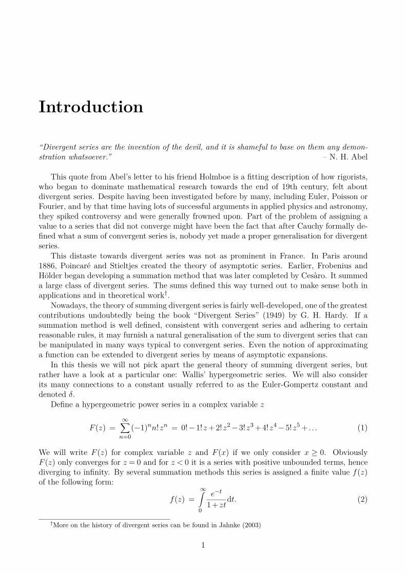


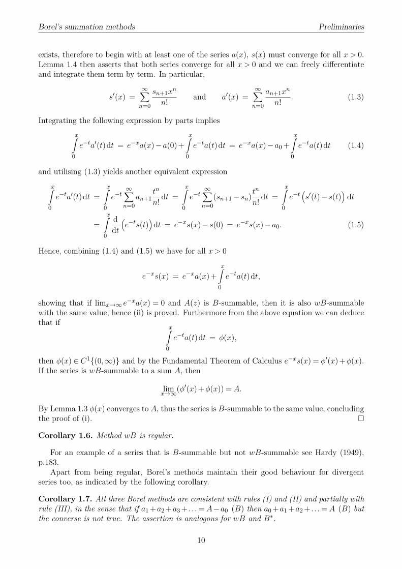
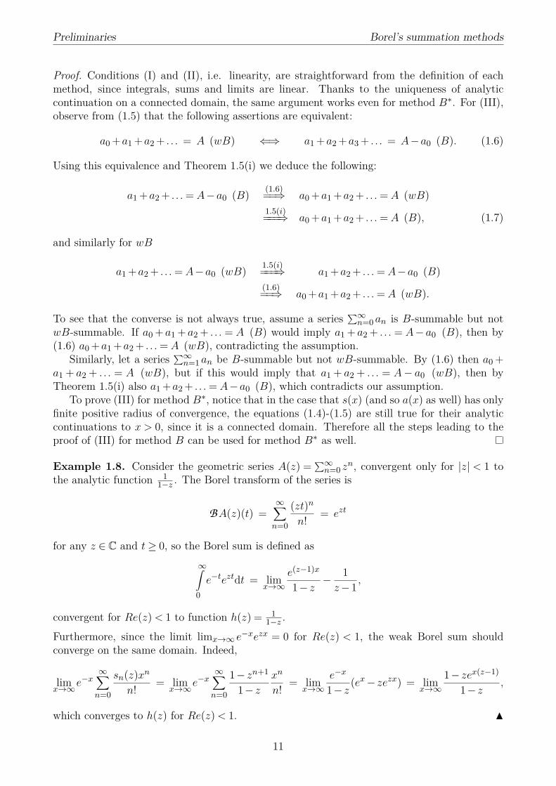


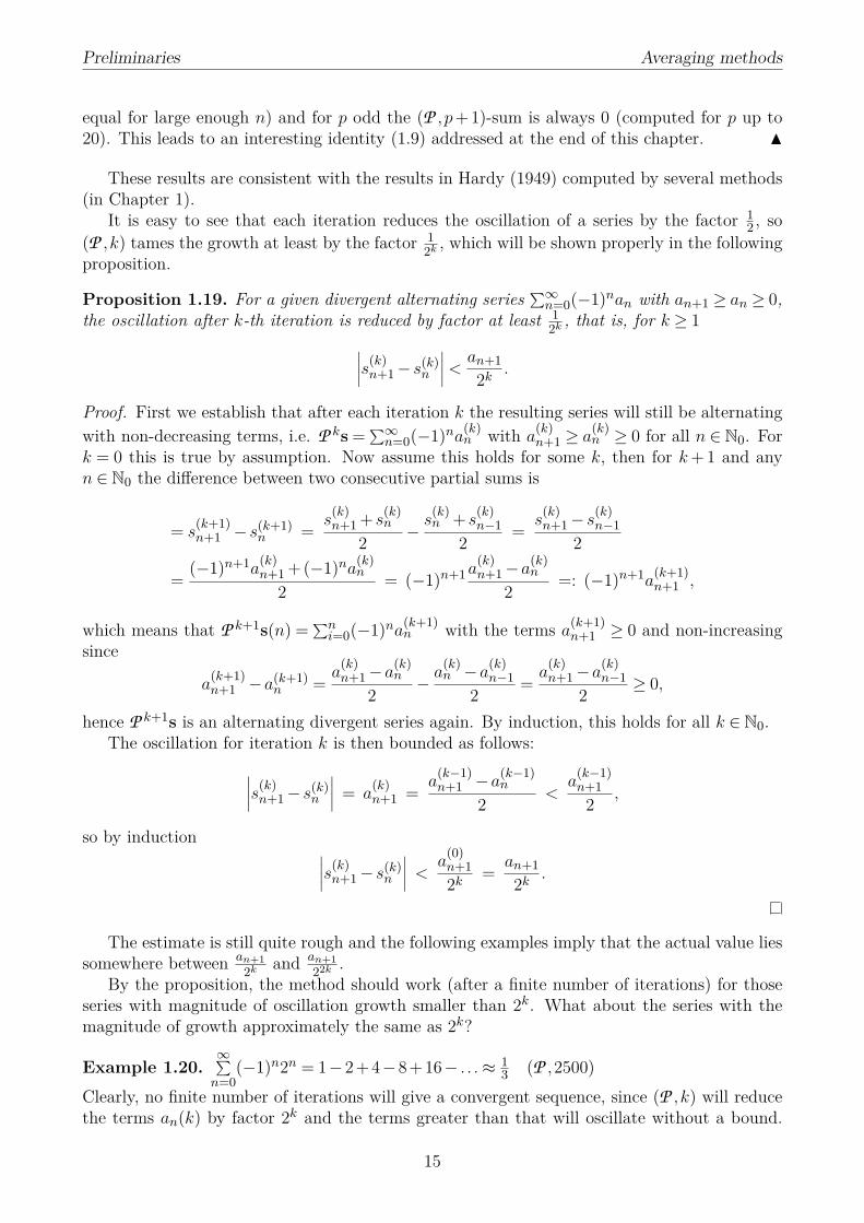
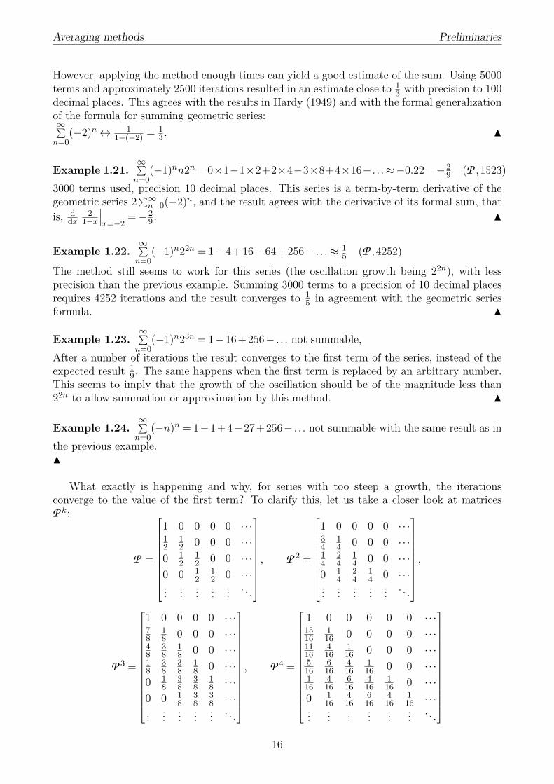


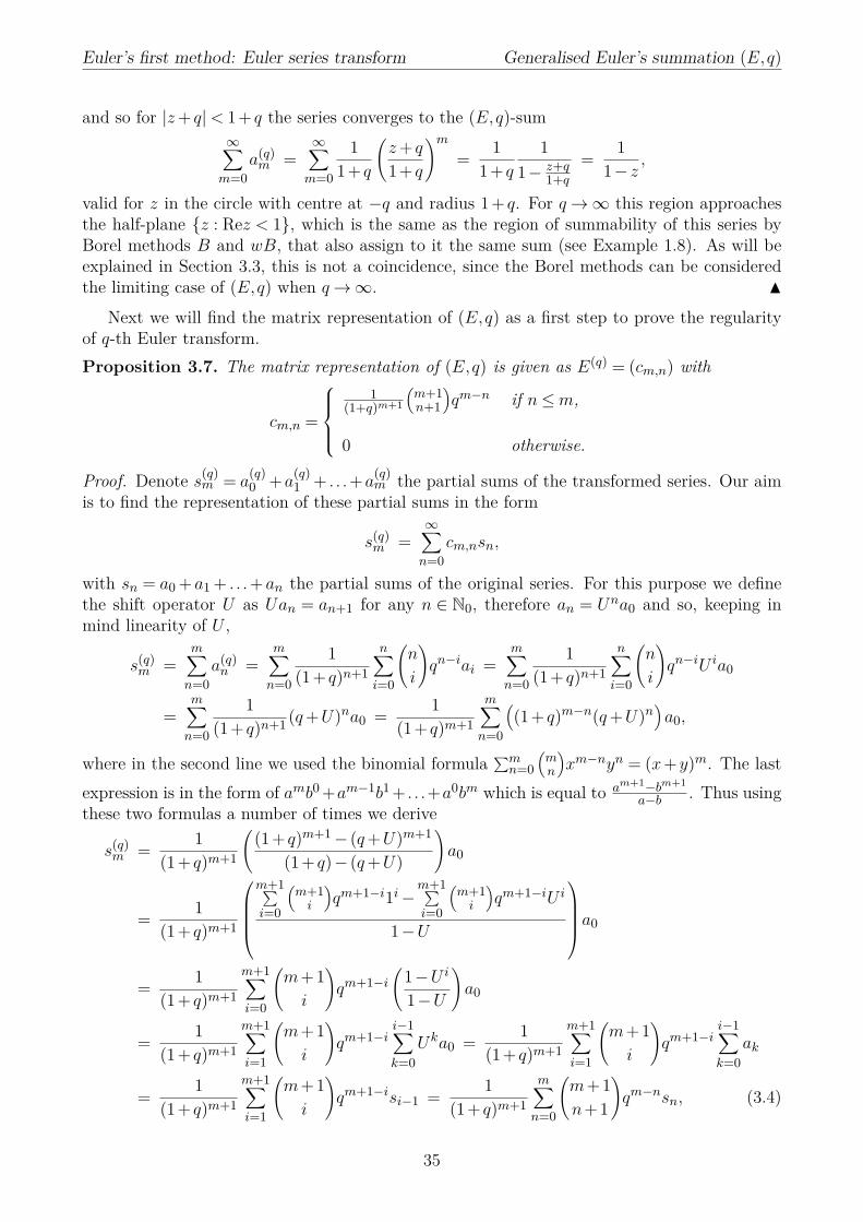


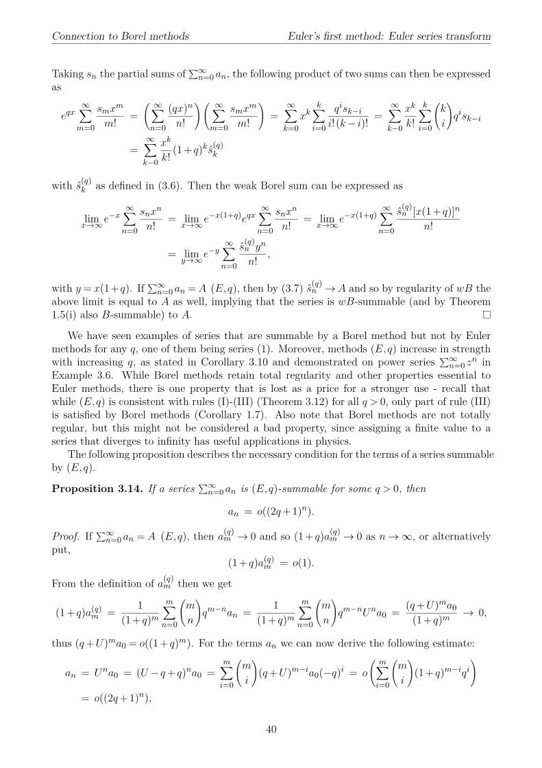


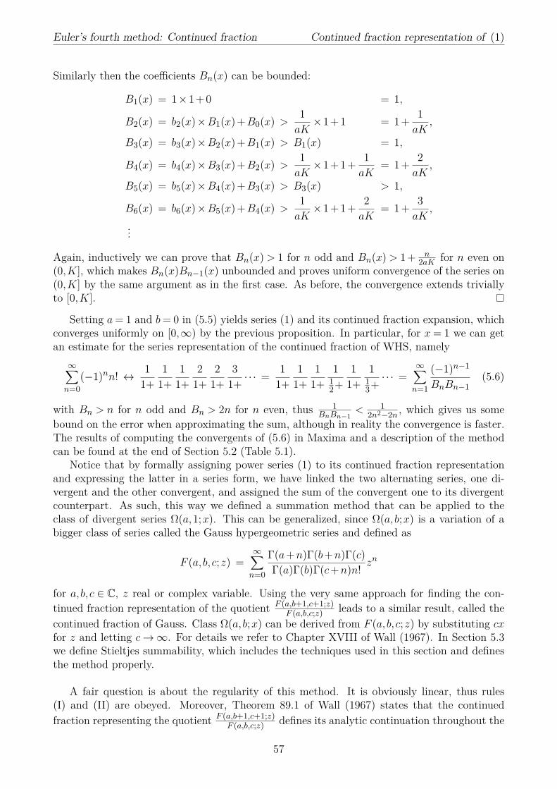
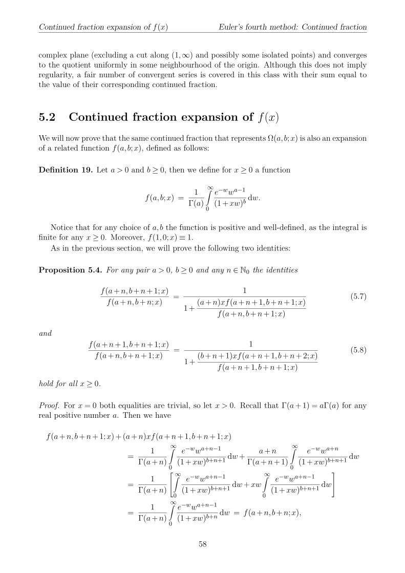
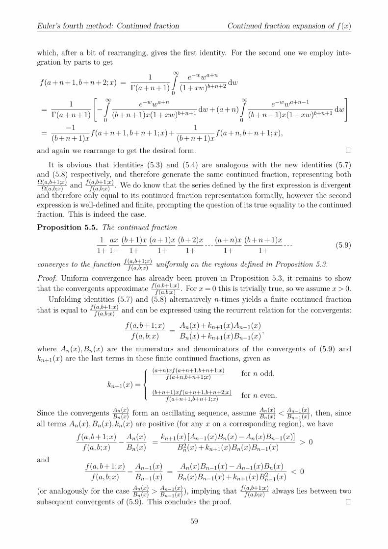


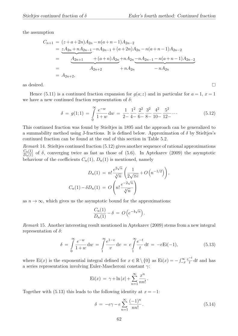


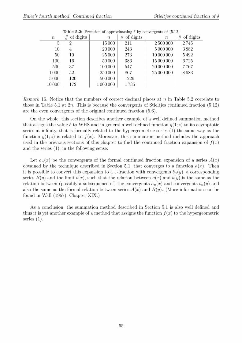

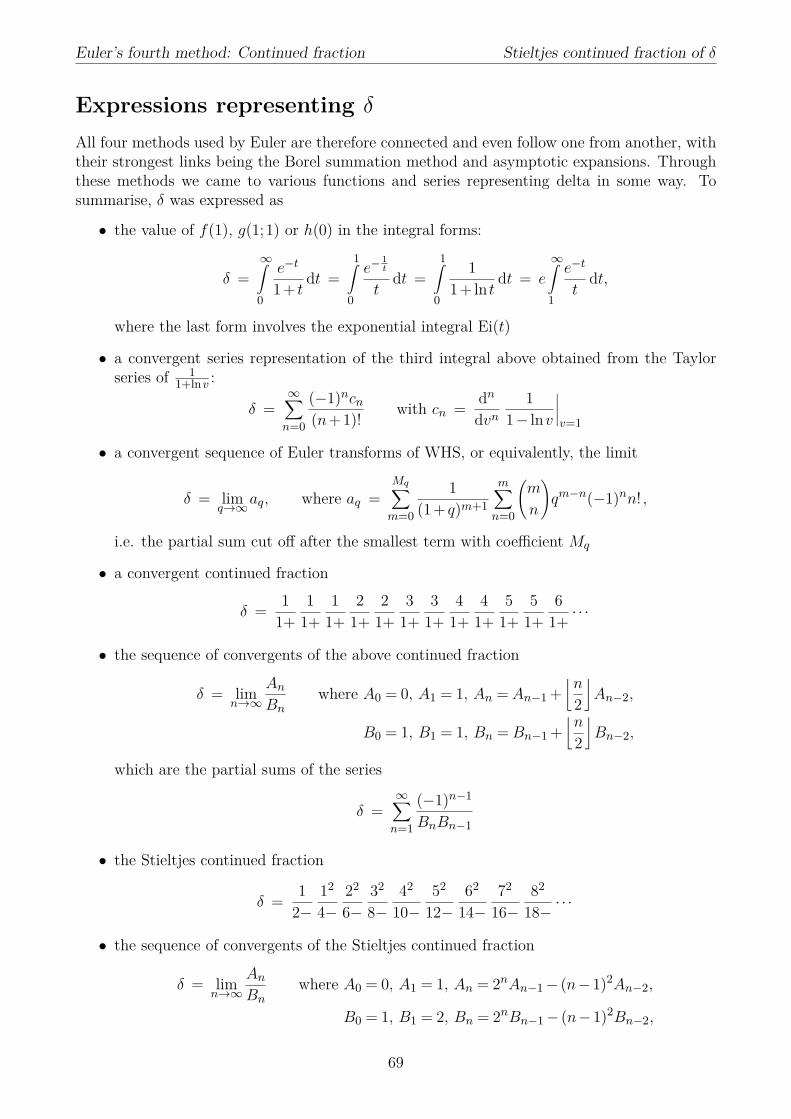
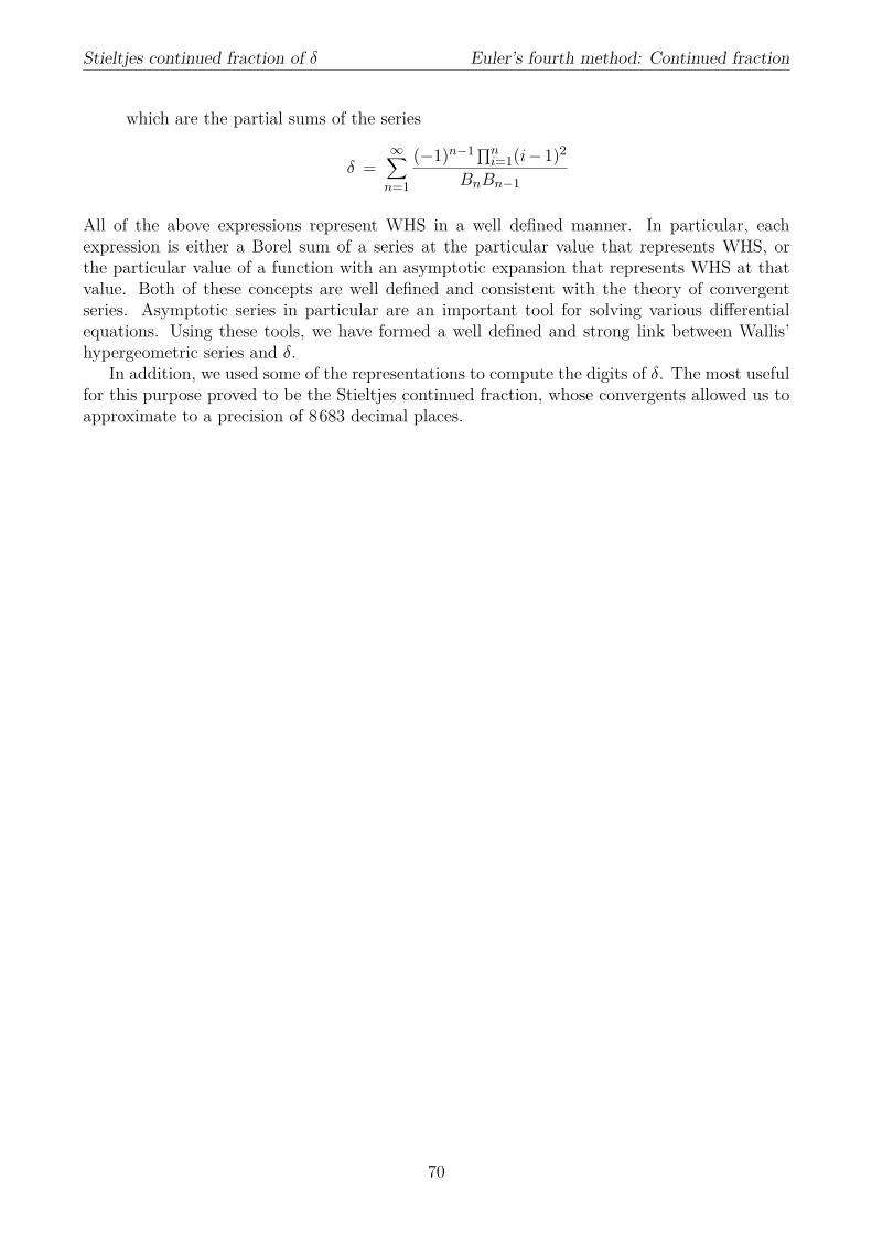


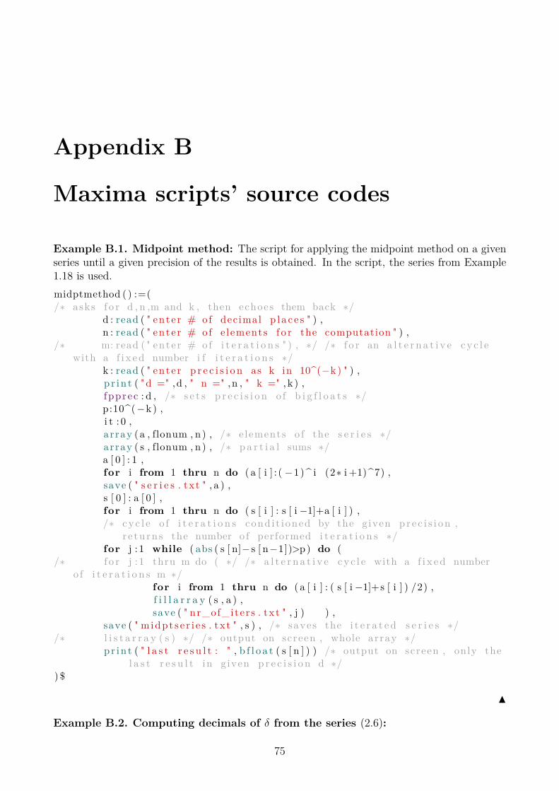
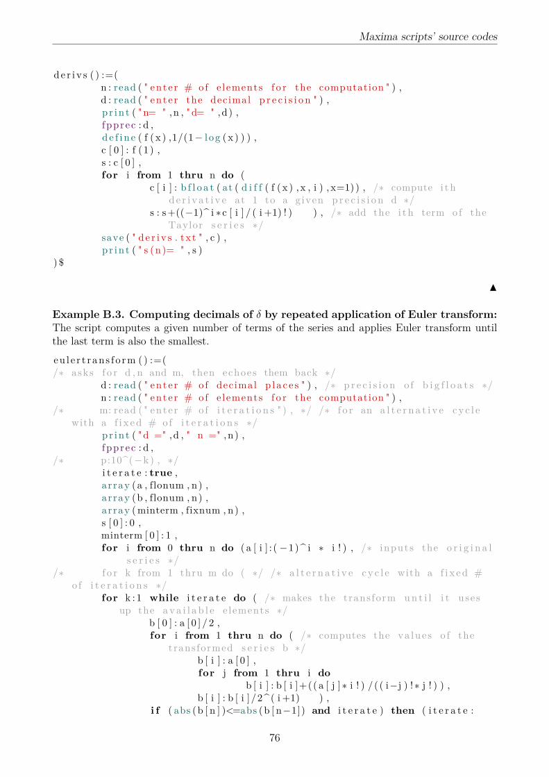

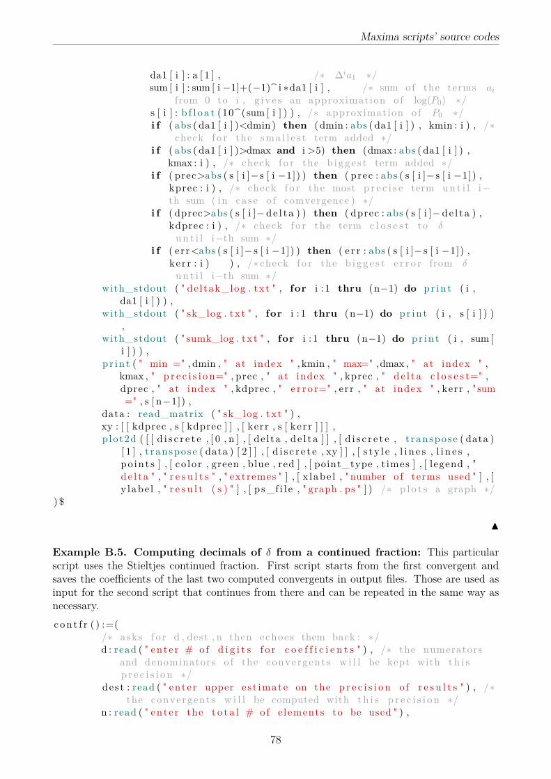


![The Euler Substitutionsuser.xmission.com/~rimrock/Documents/The Euler Substitutions.pdfa+bx+cx2 = 1 c ln [ 2cx + b + 2 c a+bx+cx2] + constant c > 0 . (1.7) The above example serves](https://static.documents.pub/doc/80x56/5f312cc56e33e933ed0fff9c/the-euler-rimrockdocumentsthe-euler-substitutionspdf-abxcx2-1-c-ln-2cx.jpg)


