FEDERAL RESERVE BANK OF SAN FRANCISCO

WORKING PAPER SERIES

The Euro Crisis in the Mirror of the EMS: How Tying Odysseus to the Mast Avoided the Sirens but Led

Him to Charybdis

Giancarlo Corsetti Cambridge University

Barry Eichengreen

University of California, Berkeley

Galina Hale Federal Reserve Bank of San Francisco

Eric Tallman

Federal Reserve Bank of San Francisco

February 2019

Working Paper 2019-04

https://www.frbsf.org/economic-research/publications/working-papers/2019/04/

Suggested citation:

Corsetti, Giancarlo, Barry Eichengreen, Galina Hale, Eric Tallman. 2019. “The Euro Crisis in the Mirror of the EMS: How Tying Odysseus to the Mast Avoided the Sirens but Led Him to Charybdis,” Federal Reserve Bank of San Francisco Working Paper 2019-04. https://doi.org/10.24148/wp2019-04 The views in this paper are solely the responsibility of the authors and should not be interpreted as reflecting the views of the Federal Reserve Bank of San Francisco or the Board of Governors of the Federal Reserve System.

1

The Euro Crisis in the Mirror of the EMS:

How Tying Odysseus to the Mast Avoided the Sirens but Led Him to Charybdis1

Giancarlo Corsetti (Cambridge University) Barry Eichengreen (University of California, Berkeley) Galina Hale2 (Federal Reserve Bank of San Francisco) Eric Tallman2 (Federal Reserve Bank of San Francisco)

February 2019

Abstract

Why was recovery from the euro area crisis delayed for a decade? The explanation lies in the absence of credible and timely policies to backstop financial intermediaries and sovereign debt markets. In this paper we add light and color to this analysis, contrasting recent experience with the 1992-3 crisis in the European Monetary System, when national central banks and treasuries more successfully provided this backstop. In the more recent episode, the incomplete development of the euro area constrained the ability of the ECB and other European institutions to do likewise.

1 This project is funded in part by the Keynes Fund at Cambridge University, with the title The Making of the Euro-Area Crisis: Lessons from Theory and History (JHLP). We also thank the Clausen Center at UC Berkeley for its financial support. 2 The views presented in this article are of the authors and don’t necessarily reflect the views of the Federal Reserve Bank of San Francisco or the Federal Reserve System.

2

1. Introduction

In the second quarter of 2017, ten years after the onset of the global financial crisis, the euro area finally started growing again. This was in contrast to countries such as the United States, where recovery commenced earlier, already in 2009, and where it was sustained more successfully.3 In this paper we assess the reasons for Europe’s delayed recovery. We adopt an historical perspective, comparing the euro area with the European Monetary System (EMS) in the 1990s. The parallels between the EMS crisis and recent events are suggestive. In both cases, countries with weak fundamentals experienced capital flight. Self-fulfilling expectations magnified and intensified currency and financial turmoil. Bond spreads rose to high levels, fragmenting financial markets across borders. In addition, the 1990s was a period of financial stress not unlike the recent episode. This was true not just of Finland and Sweden, which experienced full-blown banking crises, but also of Italy, Denmark and France. Previous analyses have underplayed the importance of banking stress in 1992-3.4 We seek to correct this in what follows. Despite these similarities in macroeconomic, financial and policy conditions, output losses from this earlier episode were modest by recent standards. Recovery from the earlier crisis was quicker. The central question asked in this paper is what accounts for these contrasting outcomes. There are a number of potential explanations for this difference in outcomes, as we detail below. But the key was the success with which national central banks and treasuries backstopped banks and sovereign debt markets in the earlier crisis, interrupting the so-called diabolic loop (Brunnermeier et al., 2016). Backstopping and recapitalizing the banks prevented financial stress from eroding economic activity, tax revenues and debt market conditions. Investment and demand were not disrupted by a liquidity squeeze and binding credit constraints to the same extent as after 2009. Hence the earlier crisis was resolved in a matter of years rather than decades. In contrast, the incomplete institutional development of the euro area limited the ability of the ECB and other European institutions to take analogous action in the recent crisis. Constrained by the euro area’s fiscal and financial rules, national governments were not able to backstop banking systems prior to the creation of the Banking Union and the European Stability Mechanism.5 National central banks, having become members of the European System of 3 As indicated by the fact that the U.S. approached full employment already in 2017. 4 Standard chronologies of banking and financial crises have omitted those years altogether, an exception being recent work at the ECB (ECB 2017). 5 The first step toward Banking Union came with the commencement of operations by the Single Supervisory Mechanism in 2014, while the European Stability Mechanism opened for business in 2012.

3

Central Banks, were not able to backstop sovereign debt markets, which in turn worsened the banks’ balance sheets and aggravated distress in the financial system. Nor was the European Central Bank prepared to provide this backstopping function prior to Mario Draghi’s “do whatever it takes” pledge in 2012. The euro crisis was magnified by this negative feedback between banks and sovereign debt markets.

2. The Setting

It is not our position that macroeconomic and financial initial conditions were identical across the two crises. There were differences as well as similarities. Understanding those differences is important for putting the key factor – the presence or absence of a financial backstop – in context. Table 1. Integration of EU-15 with the EU and the World

1988-92 2006-10 Trade (IM+EX) vs. world (incl. EU) (% of GDP) 56.8 69.7 Trade vs. EU (% of total trade) 66.2 62.6 Gross FDI (in+out) vs. world (flow) (% of GDP) 5.3 19.3 FDI vs. EU (flow) (% of total gross FDI flows)6 60.6 42.6 Capital flows vs. world (incl. EU) (millions of USD) 784,404 7,708,187

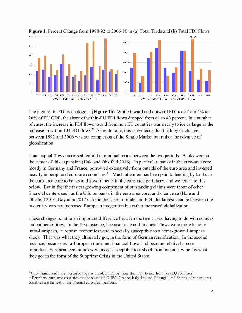
A first difference concerns the scope and direction of trade integration. Trade of the EU-15 rose between the early 1990s and the late 2000s from just under 60% to nearly 70% of GDP (Table 1).7 Meanwhile, the share of within-EU trade declined from 66% to 63%. Together these facts suggest that the biggest change affecting trade between 1992 and 2006 was not the Single Market but globalization. This expansion of trade with the rest of the world was far from symmetric across EU countries, however. As Figure 1a shows, extra-EU trade increased most dramatically for Greece, Ireland, and the Netherlands. These relatively small EU countries were disproportionately affected by globalization.8

6 Excludes outliers, namely Portugal (2002), Italy (2012), and Belgium (2008) as well as all data for Luxembourg. 7 This allows us to include the UK, which was at the center of events in 1992-3. 8 The rise in non-EU trade in Greece and the Netherlands was largely driven by import growth from China, with a subsidiary role for the post-Soviet countries. The Netherlands also saw significant growth in imports from emerging Asian countries. In Ireland’s case, the growth of trade to China was supplemented by growing trade with the Middle East.

4

Figure 1. Percent Change from 1988-92 to 2006-10 in (a) Total Trade and (b) Total FDI Flows

The picture for FDI is analogous (Figure 1b). While inward and outward FDI rose from 5% to 20% of EU GDP, the share of within-EU FDI flows dropped from 61 to 43 percent. In a number of cases, the increase in FDI flows to and from non-EU countries was nearly twice as large as the increase in within-EU FDI flows.9 As with trade, this is evidence that the biggest change between 1992 and 2006 was not completion of the Single Market but rather the advance of globalization. Total capital flows increased tenfold in nominal terms between the two periods. Banks were at the center of this expansion (Hale and Obstfeld 2016). In particular, banks in the euro-area core, mostly in Germany and France, borrowed extensively from outside of the euro area and invested heavily in peripheral euro-area countries.10 Much attention has been paid to lending by banks in the euro-area core to banks and governments in the euro-area periphery, and we return to this below. But in fact the fastest growing component of outstanding claims were those of other financial centers such as the U.S. on banks in the euro area core, and vice versa (Hale and Obstfeld 2016, Bayoumi 2017). As in the cases of trade and FDI, the largest change between the two crises was not increased European integration but rather increased globalization. These changes point to an important difference between the two crises, having to do with sources and vulnerabilities. In the first instance, because trade and financial flows were more heavily intra-European, European economies were especially susceptible to a home-grown European shock. That was what they ultimately got, in the form of German reunification. In the second instance, because extra-European trade and financial flows had become relatively more important, European economies were more susceptible to a shock from outside, which is what they got in the form of the Subprime Crisis in the United States. 9 Only France and Italy increased their within-EU FDI by more than FDI to and from non-EU countries. 10 Periphery euro area countries are the so-called GIIPS (Greece, Italy, Ireland, Portugal, and Spain), core euro area countries are the rest of the original euro area members.

5

European banks had grown substantially larger by the second half of the 2000s (Table 2). This expansion coincided with changes in bank balance sheets. In particular, the growth in deposits did not keep pace with the growth in lending. The credit-to-deposit ratio rose from 1.0 to 1.4 as banks turned to wholesale funding and to the issuance of subordinated debt.11 Table 2. Size and State of Banking Systems 1988-92 2006-10 Bank deposits/GDP (ratio)12 0.70 0.95 Bank assets/GDP (ratio) 0.84 1.28 Domestic credit to private sector/GDP (ratio) 0.67 1.18 Bank credit to deposits (ratio)13 1.04 1.41

While the international role of the euro increased relative to the earlier role of the so-called legacy currencies, sterling and the dollar remained prominent on European banks’ balance sheets (Table 3). In 1992, the European banking system was short dollars and sterling and long legacy currencies. The same was true in 2010, when it was short dollars and sterling and long euros.14 There was much commentary during the recent crisis about how European banks funded themselves in dollars and sterling but lent in local currency. It is interesting to observe that the same was already true in 1992. Table 3. Currency Composition of EU Banking System Assets and Liabilities Currency 1992q4 Claims 1992q4 Liabilities 2010q4 Claims 2010q4 Liabilities Total ($tn) 2.3 2.3 15.0 11.8 Of which (%) GBP 5.1 7.4 4.0 5.1 USD 32.6 39.2 17.8 19.8 EUR 41.1 36.8 67.9 62.0 CHF 7.4 4.5 1.4 1.7 JPY 6.1 4.0 1.6 1.8

Note: Sum across EU-15 That banks were an important vehicle for cross-border flows in both episodes had two notable consequences. First, banks accumulating market-traded claims on other countries were at risk if the value of these assets collapsed.15 11 This development is not unique to Europe, as demonstrated in Hahm et. al. (2013). 12 Excluding UK due to missing data 13 Excluding Spain and the UK due to missing data 14 At the same time they were smaller, reflecting the six-fold increase in the size of the European banking system between the two periods. 15 In the more recent period, moreover, such assets had to be marked to market, heightening the fragility of balance sheets in the event of shocks.

6

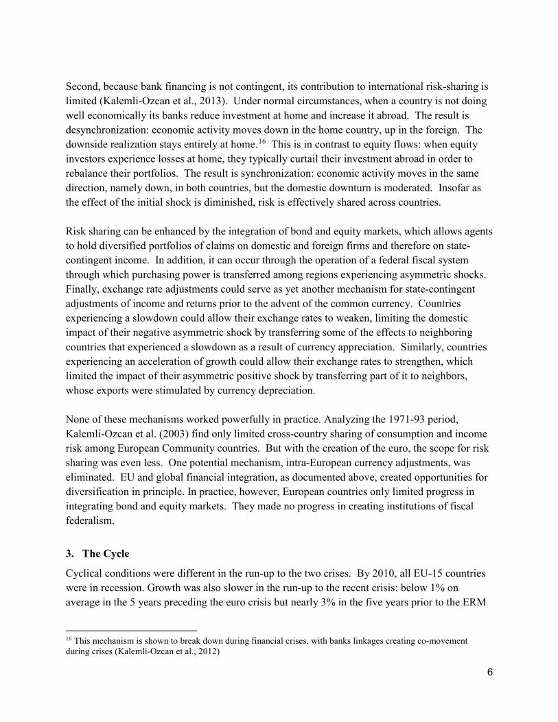
Second, because bank financing is not contingent, its contribution to international risk-sharing is limited (Kalemli-Ozcan et al., 2013). Under normal circumstances, when a country is not doing well economically its banks reduce investment at home and increase it abroad. The result is desynchronization: economic activity moves down in the home country, up in the foreign. The downside realization stays entirely at home.16 This is in contrast to equity flows: when equity investors experience losses at home, they typically curtail their investment abroad in order to rebalance their portfolios. The result is synchronization: economic activity moves in the same direction, namely down, in both countries, but the domestic downturn is moderated. Insofar as the effect of the initial shock is diminished, risk is effectively shared across countries. Risk sharing can be enhanced by the integration of bond and equity markets, which allows agents to hold diversified portfolios of claims on domestic and foreign firms and therefore on state-contingent income. In addition, it can occur through the operation of a federal fiscal system through which purchasing power is transferred among regions experiencing asymmetric shocks. Finally, exchange rate adjustments could serve as yet another mechanism for state-contingent adjustments of income and returns prior to the advent of the common currency. Countries experiencing a slowdown could allow their exchange rates to weaken, limiting the domestic impact of their negative asymmetric shock by transferring some of the effects to neighboring countries that experienced a slowdown as a result of currency appreciation. Similarly, countries experiencing an acceleration of growth could allow their exchange rates to strengthen, which limited the impact of their asymmetric positive shock by transferring part of it to neighbors, whose exports were stimulated by currency depreciation. None of these mechanisms worked powerfully in practice. Analyzing the 1971-93 period, Kalemli-Ozcan et al. (2003) find only limited cross-country sharing of consumption and income risk among European Community countries. But with the creation of the euro, the scope for risk sharing was even less. One potential mechanism, intra-European currency adjustments, was eliminated. EU and global financial integration, as documented above, created opportunities for diversification in principle. In practice, however, European countries only limited progress in integrating bond and equity markets. They made no progress in creating institutions of fiscal federalism.

3. The Cycle

Cyclical conditions were different in the run-up to the two crises. By 2010, all EU-15 countries were in recession. Growth was also slower in the run-up to the recent crisis: below 1% on average in the 5 years preceding the euro crisis but nearly 3% in the five years prior to the ERM

16 This mechanism is shown to break down during financial crises, with banks linkages creating co-movement during crises (Kalemli-Ozcan et al., 2012)

7

crisis. Among other things, this low growth constrained tax revenues, heightening concerns about the creditworthiness of sovereigns. Weak growth in 2010 was not limited to Europe, of course. As Figure 2 shows, following the Lehman crisis on September 2018, global growth fell from 5.2% in the first quarter of 2006 to just -1.9% in first quarter of 2009. During the ERM crisis, by comparison, global growth declined gradually from the same 5.2% rate in the first quarter of 1988 to 1.9% in the first quarter of 1994. Figure 2. Global GDP Growth

Whereas the average unemployment rate in the EU-15 was similar in the periods leading up to the two crises, the cross-country dispersion of rates was greater around the time of the more recent crisis (Figure 3).17 Its architects had anticipated that the euro would be an engine of convergence. Gauged by the development of unemployment rates, the opposite was true.18

17 The chart also shows dispersion of unemployment across US states, for comparison. 18 Explanations for this divergence are beyond the scope of the present paper. For a start on an analysis see Eichengreen (2019).

8

Figure 3. Unemployment Rate Divergence in the U.S. vs. the EU-15

Note: Graphed here are side-by-side box-and-whisker plots for each quarter in the sample, where the lines represent the dispersion of the data, and the dots mark outliers from our distribution. While imbalances across EU member countries in the mid-2000s had the same sign as in the early 1990s (Figure 4), they were larger. Relatively high returns on investment in the peripheral countries attracted capital inflows from the core countries, whose banks and securities markets were larger and could intermediate even greater flows than two decades before. As additional spending in the periphery enabled by these inflows fed through into higher wages, the peripheral countries lost competitiveness, and their trade deficits widened. Figure 4. Current Account Balance (a) Intra-EU and (b) Extra-EU

9

Table 4. Macroeconomic Conditions in EU-15 Prior to ERM and Euro Crises 1988-92 2006-10

Real GDP growth rate (%) 2.9 0.9 Unemployment rate (%) 7.6 7.6 Inflation rate (CPI) (%) 5.4 2.0 Policy rate (interest rate) (%) Real policy rate (%)

13.5 8.1

2.6 0.6

Government debt/GDP (%) 61.9 66.0 Government deficit/GDP (%)19 -2.3 -3.1 Current account (% of GDP) —excluding DEU and NLD

0.2 -0.2

-0.5 -1.5

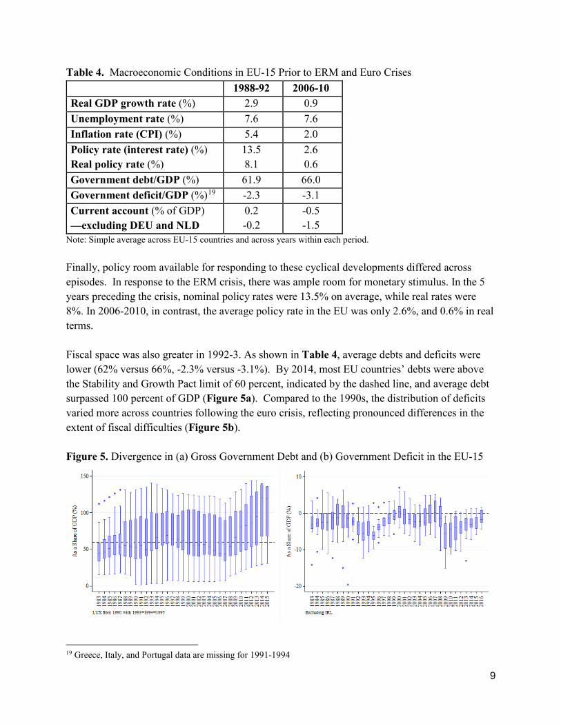
Note: Simple average across EU-15 countries and across years within each period. Finally, policy room available for responding to these cyclical developments differed across episodes. In response to the ERM crisis, there was ample room for monetary stimulus. In the 5 years preceding the crisis, nominal policy rates were 13.5% on average, while real rates were 8%. In 2006-2010, in contrast, the average policy rate in the EU was only 2.6%, and 0.6% in real terms. Fiscal space was also greater in 1992-3. As shown in Table 4, average debts and deficits were lower (62% versus 66%, -2.3% versus -3.1%). By 2014, most EU countries’ debts were above the Stability and Growth Pact limit of 60 percent, indicated by the dashed line, and average debt surpassed 100 percent of GDP (Figure 5a). Compared to the 1990s, the distribution of deficits varied more across countries following the euro crisis, reflecting pronounced differences in the extent of fiscal difficulties (Figure 5b). Figure 5. Divergence in (a) Gross Government Debt and (b) Government Deficit in the EU-15

19 Greece, Italy, and Portugal data are missing for 1991-1994

10

The EMS and euro crises had important similarities, as we stressed in our introduction. But a nuanced comparison also requires acknowledging their differences, as we have done here.

4. The Crisis

The shock triggering the ERM crisis was monetary contraction and demand expansion in Germany. Deficit spending on transfers to the new eastern lander following German reunification boosted domestic demand. To limit inflation, the Bundesbank raised interest rates. Any positive spillover from higher German demand was counterbalanced by the negative effect of higher interest rates, which were transmitted to other ERM countries by the combination of pegged exchange rates and free international capital flows. In many cases, this second, negative spillover dominated. In 2008 the trigger was not an asymmetric demand shock in Europe itself, but the financial crisis originating in the United States, to which Europe was subject as a result of its growing extra-European links (see Section 2 above). This time, instead, an asymmetric financial response followed. Banks in core Europe lost their access to funding and incurred losses on their U.S. asset-backed securities. In response, they curtailed their lending to the European periphery. The reversal of private capital flows, which had financed the current account deficits of the euro-area periphery prior to the crisis, meant that those deficits now had to be reduced. Historically, countries in similar situations had been able to achieve quick current account improvements by depreciating their currencies. This obviously was not an option in the context of a currency union. The monetary policy reaction to the ERM crisis was substantial, with policy rates declining from an average of 13.5 to an average of 8.7 percent between the five years through 1992 and five following years. Given that inflation fell by less, from 5.4 to 2.8 percent, this implies that real policy rates declined from 8.1 to 5.9 percent (Table 5).

11

Table 5. Monetary and Fiscal Policy, Spread, and Current Account Indicators 1988-92 1993-97 2006-10 2011-15

Policy rate (interest rate) (%) Real policy rate (%)

13.5 8.1

8.7 5.9

2.6 0.6

0.5 -0.7

Current account (% of GDP) —excluding DEU and NLD

0.2 -0.2

1.5 1.4

-0.5 -1.5

2.1 1.1

Government debt/GDP (%) 61.9 72.8 66.0 88.9 Government deficit/GDP (%)20 -2.3 -4.1 -3.1 -3.6 5-year Government Bond Yield (%) —in real terms

9.7 4.3

7.0 4.2

3.4 1.4

3.0 1.8

Note: Simple average across EU-15 countries and across years within each period. When the euro crisis erupted in 2010, in contrast, the ECB deposit rate was already at its lowest level in history, 0.25 percent, leaving little room to reduce rates further (Table 5). Not until much later, in 2014-5, did the ECB attempt to circumvent the zero lower bound by experimenting with negative policy rates and large-scale quantitative easing. Even then, a single monetary policy was a blunt instrument for addressing the different needs of different member countries. Given the relatively heavy economic weight of the core countries in euro area aggregates, and with the ECB making monetary policy with the euro area average in mind, policy rates were nearer to what was suitable to economic conditions of the core countries than to those in the periphery (Nechio 2011; Malkin and Nechio, 2012). Once the ERM peg was abandoned, other currencies depreciated against both the deutschemark and the dollar (Figure 6). Depreciation reduced or eliminated current account deficits that were now more difficult to finance. Whereas roughly half of ERM members had been running current account deficits prior to the crisis, in most cases their current accounts quickly shifted into surplus as a result of the shift in relative prices. Impressively, this adjustment was already complete by 1993.

20 Greece, Italy, and Portugal data are missing for 1991-1994.

12

Figure 6. Nominal Exchange Rates against the USD

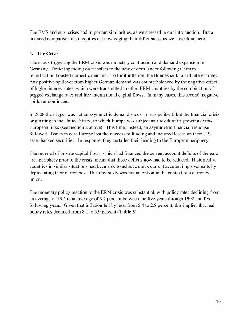
The same response was not available in 2010, since there existed only a single exchange rate for the euro area. The euro depreciated by 14.2 percent in nominal terms against the dollar between the third quarter of 2008 and the second quarter of 2010. But this was far from enough to relieve balance-of-payments pressure on the peripheral countries. Still, current accounts had to be compressed one way or another given the sudden stop in capital inflows. This was accomplished through internal devaluation and the compression of domestic spending and import demand. The resulting fall in nominal wages in the peripheral countries (by 21% in Greece, and 6-8% in Ireland, Portugal, and Spain) achieved the necessary current account adjustment by the end of 2012, but at the cost of further depressing consumption and demand and delaying the subsequent recovery. Much attention has been paid to the role of emergency financial assistance from the International Monetary Fund, the European Commission and the European Central Bank. But as Figure 7 shows, this in fact eliminated only a small fraction of the current account adjustment required of the crisis countries.

13

Figure 7. Composition of Net Foreign Liabilities of GIIPS.

In the 1990s, a number of countries experienced substantial banking difficulties, but given the relatively limited size of bank balance sheets, the financial impact was, with a few exceptions, readily contained. Finland and Sweden experienced the most serious crises: Laeven and Valencia (2013) put the total fiscal costs at 13% for Finland and 4% of GDP for Sweden. In 1993, Danmarks Nationalbank was forced to provide standby liquidity support for the country’s second largest bank and was involved in finding solutions for five other distressed banks. Interventions to backstop the Italian banking system between 1990 and 1996 cost the Italian government about one-half percent of 1996 GDP (Duca et al. 2017). Credit Lyonnais was bailed out by the French government in early 1994 after having incurred substantial losses in the preceding year. Other than the cases of Finland and Sweden, none of these difficulties rose to the level of systemic crises, but they could have posed serious problems for financial intermediation and economic activity had they not been successfully contained. In the more recent episode, banks were substantially larger, making for correspondingly higher costs when they had to be bailed out. When the subprime bubble burst, banks in the core countries suffered heavy losses on their investments in U.S. asset-backed securities, as noted. Large core-country banks were already undercapitalized prior to the crisis, as a result of light-touch regulation, zero capital charges on investments in sovereign bonds, and the ability to book investments off balance sheet where they escaped capital requirements.21 Hence banks did not have sufficient capital to cover their losses, absent government support. Those losses not only weakened their balance sheets but also aggravated existing currency mismatches, because losses meant a reduction of the dollar value of bank assets without corresponding reductions in bank liabilities. When the euro began depreciating against the

21 In the most extreme case, the ratio of equity to total assets was under 2 percent for Deutsche Bank prior to 2008.

14

dollar, this further compounded the problem, which grew still worse with the need to rebalance the currency composition of balance sheets by purchasing appreciated dollars.22 Figure 8. Share of Domestic Debt in Domestic Banks23

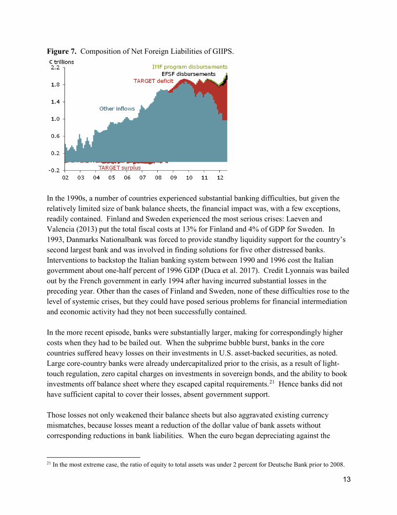
It was at this point that the diabolic loop connecting banking problems and sovereign debt problems came into play. Banks in the euro-area periphery had invested heavily in their own governments’ debt securities (Figure 8). Falling government-bond prices therefore caused them balance-sheet losses, owing to recently adopted mark-to-market requirements intended to increase transparency.24 The large size of banking systems exacerbated the problem in two ways. First, attempts to bail out troubled banks put substantial stress on public finances: recapitalization and other restructuring costs ranged from 1% of GDP in France to 40% in Ireland (Laeven and Valencia, 2013) – contrast “just” 13 percent in Finland in the 1990s. Combined with high inherited debts, this created pressure for larger fiscal consolidations in subsequent years, given the debt break enshrined in the European treaties. And fiscal consolidation there was, as shown in Figure 9. Second, because peripheral sovereign debt was concentrated in the balance sheets of banks in the originating countries, there existed a direct link between the condition of the public finances and the condition of the banks. The worsening balance-sheet condition of the banks and requisite

22 The currency swap arranged between the Federal Reserve and the ECB was intended to alleviate this problem to some extent by providing ample dollar liquidity to European banks, but did not help with balance sheet effects of dollar appreciation. 23 Sovereign debt of a country that is held in EBA-reporting banks of the same country in 2010 as a share of sovereign debt held by all EBA-reporting banks in the euro area. 24 Because banks in the periphery were substantially financed by banks in the core, these problems also affected the condition of core banks.

15

bailouts had first worsened the fiscal situation of the government. But the worsening fiscal situation of the government now worsened the balance sheets of the banks, as sovereign bond prices declined, requiring further fiscal injections to the banking system, worsening sovereign balance sheets and raising questions about whether governments would have the capacity to continue backstopping the banks. Figure 9. Fiscal Consolidation as a Percent of GDP25

In the earlier crisis, bank restructuring had substantial fiscal costs only in a handful of countries, as we saw above. As a result, there was less upward pressure on government bond yields (Table 5). Yields actually fell below pre-crisis levels as early as 1994 (Figure 10). The fall in yields further limited the rise in debt ratios and had the additional benefit of protecting bank balance sheets from losses on government security holdings.26 Thus, even in countries with impaired banks, the doom loop between government debt and banking crises remained inactive, and the operation of the financial accelerator was contained.

25 Fiscal consolidation is defined as measures intended to reduce deficit, based on narrative analysis. 26 Even if the assets are not marked to market on the balance sheet, a decline in their value leads to reduction of the banks’ franchise value and results in increased cost of raising external equity and debt.

16

Figure 10. 5-year Government Bond Yield

The rise in peripheral government sovereign debt yields in 2010 was both larger and more prolonged, with average euro area periphery sovereign yields (even excluding Greece) only converging to the average level of core sovereigns by the end of 2014. Yields began their descent only after Draghi’s do-whatever-it-takes pledge (Figure 10), more than two years into the crisis. By this time sovereign debt problems had been allowed to undermine the condition of the banks – the doom loop had already been set in motion. This impaired the ability of the governments to borrow and apply fiscal stimulus, which in turn raised questions about the development of tax revenues and public creditworthiness and, on the banking side, nonperforming loans. Indeed, in an effort to control the run-up in sovereign yields, the authorities pivoted already in 2010 to fiscal consolidation (Table 5). But in contrast to 1992-3, this fiscal consolidation did not lead to the decline of sovereign yields, given limited scope for interest rate reductions and currency depreciation to offset the contractionary effects. By the end of 1995, the ERM crisis was effectively resolved. A majority of ERM members re-affirmed their commitment to adopt a single currency, while others, notably the UK, Sweden and Denmark, opted for remaining outside the currency area and instead embraced inflation targeting as their monetary framework.27 In contrast, in 2019, the time of writing, the euro crisis still remains unresolved, in the limited sense that economic growth in the euro area still needs the full monetary policy support of the ECB.

27 Denmark constituted a third category, as a country that chose to remain out of the single currency but adopted an exchange rate target (against the deutschmark and then the euro) rather than an inflation target.

17

5. Lessons

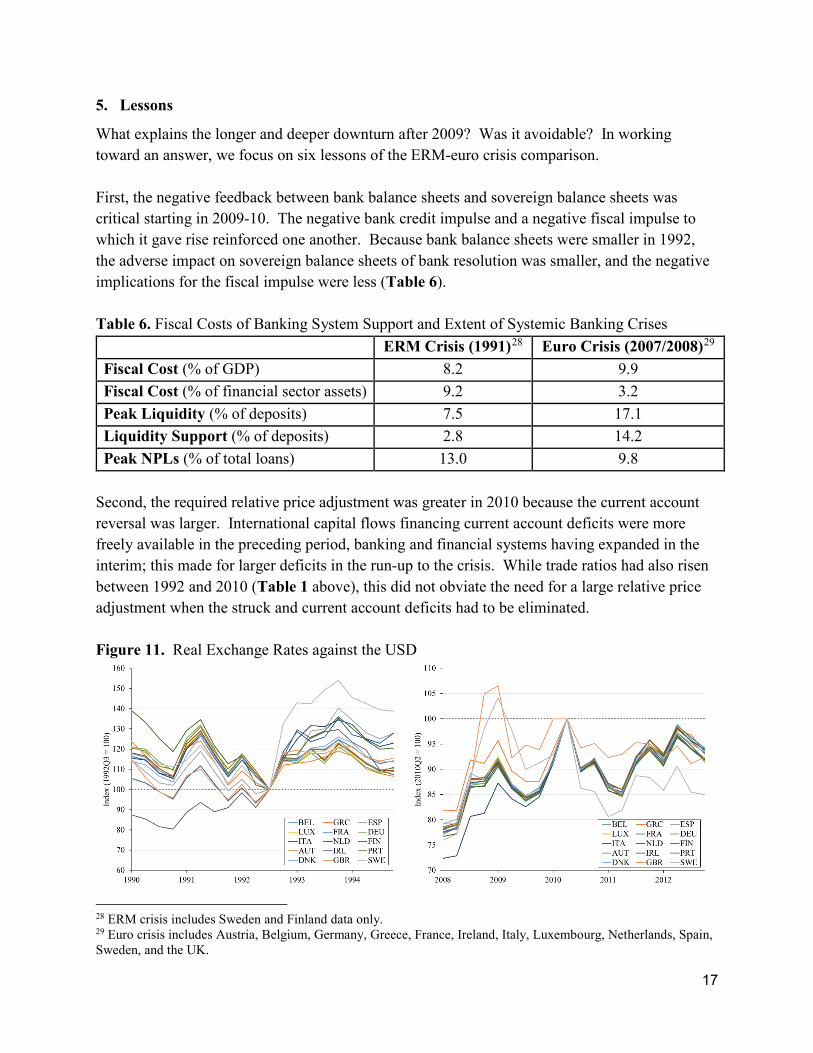
What explains the longer and deeper downturn after 2009? Was it avoidable? In working toward an answer, we focus on six lessons of the ERM-euro crisis comparison. First, the negative feedback between bank balance sheets and sovereign balance sheets was critical starting in 2009-10. The negative bank credit impulse and a negative fiscal impulse to which it gave rise reinforced one another. Because bank balance sheets were smaller in 1992, the adverse impact on sovereign balance sheets of bank resolution was smaller, and the negative implications for the fiscal impulse were less (Table 6). Table 6. Fiscal Costs of Banking System Support and Extent of Systemic Banking Crises ERM Crisis (1991)28 Euro Crisis (2007/2008)29

Fiscal Cost (% of GDP) 8.2 9.9 Fiscal Cost (% of financial sector assets) 9.2 3.2 Peak Liquidity (% of deposits) 7.5 17.1 Liquidity Support (% of deposits) 2.8 14.2 Peak NPLs (% of total loans) 13.0 9.8

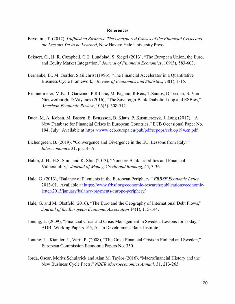
Second, the required relative price adjustment was greater in 2010 because the current account reversal was larger. International capital flows financing current account deficits were more freely available in the preceding period, banking and financial systems having expanded in the interim; this made for larger deficits in the run-up to the crisis. While trade ratios had also risen between 1992 and 2010 (Table 1 above), this did not obviate the need for a large relative price adjustment when the struck and current account deficits had to be eliminated. Figure 11. Real Exchange Rates against the USD

28 ERM crisis includes Sweden and Finland data only. 29 Euro crisis includes Austria, Belgium, Germany, Greece, France, Ireland, Italy, Luxembourg, Netherlands, Spain, Sweden, and the UK.

18

Third, this relative price adjustment (Figure 11) was more difficult to achieve in 2010. Individual euro-area countries no longer had their own exchange rate to depreciate. Since the exchange rate of the euro was influenced by conditions in the core countries, which make up the largest part of the euro area, the exchange rate did not depreciate to the extent required to facilitate relative price adjustment in the periphery. In the wake of the 1992-3 crisis, most policy models of central banks and treasuries predicted that currency depreciation would be offset by double-digit inflation. In the event, inflation rose by only a few percentage points. Still, this temporary rise in inflation contributed to macroeconomic adjustment. It facilitated relative wages and price adjustments, because wages could rise in expanding sectors without having to fall in contracting ones. Fourth, and relatedly, government debts and deficits were lower in 1992-3, leaving more room for supportive fiscal policy to prevent the kind of deep recession that might have activated the doom loop. Because fiscal burdens were lighter and governments had national central banks to backstop the sovereign debt market in this earlier crisis, sovereign spreads were less sensitive to the fiscal outlook. Pooled regressions documenting the contrast are reported in Table 7. Table 7. Sensitivity of Sovereign Spreads to Changes in Government Debt

Fifth, to the extent that domestic cost and price reductions lagged in 2009-10, the required compression of current account deficits could only occur through reductions in imports, brought about by public spending cuts by governments and deleveraging by households. This made for less demand, deeper recessions, weaker tax revenues and more nonperforming loans, aggravating balance-sheet problems for firms, banks and governments alike.

19

Sixth, central banks of countries experiencing these problems in 1992-3 could cut interest rates to support domestic demand and prevent balance-sheet problems from spiraling out of control. They could backstop the sovereign as well as the banks. In 2009-10, in contrast, policy rates were set by the ECB in light of euro-area-wide conditions, not crisis-country conditions, which meant that they were higher than warranted by state of this last set of countries. Moreover, the transmission of monetary policy differed across countries in perverse ways: the same policy rate translated into very different borrowing costs for firms and governments of different countries as their credit worthiness diverged. From these six lessons follows the bottom line. Managing large shocks requires a credible backstop for banks and sovereign debt markets. This backstop is required to prevent the endogenous amplification of shocks. A backstop was available during the ERM crisis but not the euro crisis. The goal of euro-area reform now should be to provide one.

20

References

Bayoumi, T. (2017), Unfinished Business: The Unexplored Causes of the Financial Crisis and the Lessons Yet to be Learned, New Haven: Yale University Press.

Bekaert, G., H. R. Campbell, C.T. Lundblad, S. Siegel (2013), “The European Union, the Euro,

and Equity Market Integration,” Journal of Financial Economics, 109(3), 583-603. Bernanke, B., M. Gertler, S.Gilchrist (1996), “The Financial Accelerator in a Quantitative

Business Cycle Framework,” Review of Economics and Statistics, 78(1), 1-15. Brunnermeier, M.K., L.Garicano, P.R.Lane, M. Pagano, R.Reis, T.Santos, D.Tesmar, S. Van

Nieuwerburgh, D.Vayanos (2016), “The Sovereign-Bank Diabolic Loop and ESBies,” American Economic Review, 106(5), 508-512.

Duca, M, A. Koban, M. Basten, E. Bengsson, B. Klaus, P. Kusmierczyk, J. Lang (2017), “A

New Database for Financial Crises in European Countries,” ECB Occasional Paper No. 194, July. Available at https://www.ecb.europa.eu/pub/pdf/scpops/ecb.op194.en.pdf

Eichengreen, B. (2019), “Convergence and Divergence in the EU: Lessons from Italy,”

Intereconomics 31, pp.14-19. Hahm, J.-H., H.S. Shin, and K. Shin (2013), “Noncore Bank Liabilities and Financial

Vulnerability,” Journal of Money, Credit and Banking, 45, 3-36. Hale, G. (2013), “Balance of Payments in the European Periphery,” FRBSF Economic Letter

2013-01. Available at https://www.frbsf.org/economic-research/publications/economic-letter/2013/january/balance-payments-europe-periphery/

Hale, G. and M. Obstfeld (2016), “The Euro and the Geography of International Debt Flows,”

Journal of the European Economic Association 14(1), 115-144. Jonung, L. (2009), “Financial Crisis and Crisis Management in Sweden. Lessons for Today,”

ADBI Working Papers 165, Asian Development Bank Institute. Jonung, L., Kiander, J., Varti, P. (2008), “The Great Financial Crisis in Finland and Sweden,”

European Commission Economic Papers No. 350. Jorda, Oscar, Moritz Schularick and Alan M. Taylor (2016), “Macrofinancial History and the

New Business Cycle Facts,” NBER Macroeconomics Annual, 31, 213-263.

21

Kalemli-Ozcan, S., E. Papaioannou, F. Perri (2012), “Global Banks and Crisis Transmission,” Journal of International Economics 89 (2), 495-510.

Kalemli-Ozcan, S., E. Papaioannou, J.-L. Peydró (2010), “What Lies Beneath the Euro's Effect

on Financial Integration: Currency Risk, Legal Harmonization, or Trade?” Journal of International Economics 81(1), 75-88.

Kalemli-Ozcan, S., E. Papaioannou, J.-L. Peydró (2013), “Financial Regulation, Financial

Globalization, and the Synchronization of Economic Activity,” Journal of Finance 68 (3), 1179-1228.

Kalemli-Ozcan, S., B. E. Sorensen, O. Yosha (2003), “Risk Sharing and Industrial

Specialization: Regional and International Evidence,” American Economic Review 93(3), 903-918.

Laeven, L. and F. Valencia (2013) “Systematic Banking Crises Database” IMF Economic

Review 61, 225-270. Laeven, L., and F. Valencia (2018), “Systematic Banking Crises Revisited,” IMF Working Paper

18/206, International Monetary Fund. Lane, P. R. and G. M. Milesi-Ferretti, “The External Wealth of Nations Mark II: Revised and

extended estimates of foreign assets and liabilities, 1970–2004,” Journal of international Economics 73.2 (2007): 223-250.

Logan, A. (2001), “The United Kingdom’s Small Banks’ Crisis of the early 1990s: What were

the Leading Indicators of Failure,” Bank of England Working Paper. Malkin I. and F. Nechio (2012), “U.S. and Euro Area Monetary Policy by Region,” FRBSF

Economic Letter 2012-06. Nechio, F. (2011), “Monetary Policy when One Size does not Fit All,” FRBSF Economic Letter

2011-18. Pescatori, A., D. Leigh, J. Guajardo, P. Devries (2011), “A New Action-Based Dataset of Fiscal

Consolidation,” IMF Working Paper 11/128, International Monetary Fund. Reinhart, C. and K. Rogoff (2015), “Financial and Sovereign Debt Crises: Some Lessons

Learned and Those Forgotten,” Journal of Banking and Financial Economics 2 (4): 5-17.

22

von Hagen, J., A. H. Hallett and R. Strauch (2002), “Budgetary Consolidation in Europe: Quality, Economic Conditions, and Persistence,” Journal of the Japanese and International Economies 16(4), 512-535.

23

Appendix: Data sources and definitions

Table 1. Integration of EU-15 with the EU and the World: Trade vs. world: IMF’s Direction of Trade Statistics Trade vs EU: IMF’s Direction of Trade Statistics Gross FDI vs. world (flow): World Bank/IMF’s Balance of Payment statistics and UNCTAD FDI vs. EU (flow): OECD Capital flows vs. world: Lane and Milesi-Ferretti (2007)

Figure 1a. Trade Flows: IMF’s Direction of Trade Statistics Figure 1b. FDI Flows: OECD/World Bank Table 2. Size and State of the Banking Systems: World Bank Global Financial Development database Table 3. Currency composition of EU banking system assets and liabilities: Bank of International Settlements Figure 2. Global GDP Growth: IMF’s International Finance Statistics Figure 3. Unemployment Rate Divergence: EU data from IMF’s International Financial Statistics and FRED; U.S. data from Haver Analytics/Bureau of Labor Statistics Figure 4. Current Account Balances: Jorda et al. (2016), CEIC, and Eurostat Table 4. Macroeconomic conditions in EU-15 prior to ERM and euro crises:

Real GDP growth rate: IMF’s World Economic Outlook database Unemployment rate: IMF’s International Financial Statistics and FRED Inflation rate (CPI): IMF’s International Financial Statistics, Haver Analytics/OECD, and FRED Policy Rate: Eurostat, IMF’s International Financial Statistics, Haver Analytics/OECD, and CEIC Government debt/GDP: Jorda et al. (2016), IMF’s World Economic Outlook database, FRED, and CEIC Government deficit/GDP: Eurostat and CEIC Current account: Jorda et al. (2016), CEIC, and Eurostat

Figure 5a. Government Debt: Jorda et al. (2016), IMF’s World Economic Outlook database, FRED, Statistics Austria, and CEIC Figure 5b. Government Deficit: Eurostat Table 5. Monetary and Fiscal Policy and Current Account Indicators:

Policy Rate: Eurostat, IMF’s International Financial Statistics, CEIC, and Haver Analytics/OECD Current account: Jorda et al. (2016), CEIC, and Eurostat Government debt/GDP: Jorda et al. (2016), IMF’s World Economic Outlook database, FRED, and CEIC Government deficit/GDP: Eurostat and CEIC

24

5-yr Government Bond Yield: Global Financial Data (French data supplemented from Bloomberg)

Figure 6. Nominal Exchange Rates against the Dollar: IMF’s International Financial Statistics Figure 7. Composition of net foreign liabilities of GIIPS: Hale (2013) and original data from International Monetary Fund, national central banks, European Financial Stability Facility, Eurostat Figure 8. Share of Domestic Debt in Domestic Banks: EBA 2011 Stress test Figure 9. Fiscal Consolidation as % of GDP: Pescatori et al. (2011) Figure 10. 5-yr Government Bond Yield: GFD (French data supplemented from Bloomberg). Table 6. Fiscal costs of banking system support and extent of systemic banking crises: Laeven and Valencia (2018) Figure 11. Real Exchange Rates against the Dollar: Nominal exchange rate data from the IMF’s International Financial Statistics; CPI data from the IMF’s International Financial Statistics, Haver Analytics/OECD, and Haver Analytics/BLS