The euro's influence upon trade: Rose effect versus border effect

Work ing PaPer Ser i e Sno 941 / S ePtember 2008

tHe eUro’S inFLUenCe UPon traDe

roSe eFFeCt verSUS borDer eFFeCt

by Gianluca Cafiso

WORKING PAPER SER IESNO 941 / SEPTEMBER 2008

In 2008 all ECB publications

feature a motif taken from the

10 banknote.

THE EURO’S INFLUENCE

UPON TRADE

ROSE EFFECT VERSUS

BORDER EFFECT 1

by Gianluca Cafiso 2

This paper can be downloaded without charge fromhttp://www.ecb.europa.eu or from the Social Science Research Network

electronic library at http://ssrn.com/abstract_id=1265505.

1 The views expressed are those of the author and do not necessarily reflect the views or policies of the European Central Bank. I thank Rodolfo

Helg for the helpful comments and support, and the anonymous Referee for her remarks to a previous version of this paper.

2 Department of Economics at Pavia University, Via San Felice, 5, I-27100 Pavia - Italy and temporarily at

the European Central Bank, Kaiserstrasse 29, D-60311 Frankfurt am Main, Germany;

e-mail: [email protected]; [email protected]

© European Central Bank, 2008

Address Kaiserstrasse 29 60311 Frankfurt am Main, Germany

Postal address Postfach 16 03 19 60066 Frankfurt am Main, Germany

Telephone +49 69 1344 0

Website http://www.ecb.europa.eu

Fax +49 69 1344 6000

All rights reserved.

Any reproduction, publication and reprint in the form of a different publication, whether printed or produced electronically, in whole or in part, is permitted only with the explicit written authorisation of the ECB or the author(s).

The views expressed in this paper do not necessarily refl ect those of the European Central Bank.

The statement of purpose for the ECB Working Paper Series is available from the ECB website, http://www.ecb.europa.eu/pub/scientific/wps/date/html/index.en.html

ISSN 1561-0810 (print) ISSN 1725-2806 (online)

3ECB

Working Paper Series No 941September 2008

Abstract 4

Non-technical summary 5

1 Introduction 7

2 Data description 9

3 Rose effect estimations 10

4 Border effect estimations 15

4.1 Econometrics of the border effect 16

4.2 Estimations of the border effect 17

5 Robustness checks 21

6 Conclusions 22

Appendices 25

Bibliographical references 31

European Central Bank Working Paper Series 34

CONTENTS

4ECBWorking Paper Series No 941September 2008

AbstractThis paper assesses the Euro’s influence upon European trade by estimating two different indicators. The first is the so-called “Rose Effect”, while the second is the “Border Effect”. The former measures how much a country within a currency union trades more with its partners than with non-member countries, the latter measures the integration of a country with its trade partners. This study of the Euro’s influence by means of the Border Effect is a novelty in the literature, it reveals that the Euro’s influence upon trade is not so clear as papers focused only on the Rose Effect claim. This casts doubts about the consequences of the Euro introduction for the European Single Market. Both indicators are estimated by means of a gravity model for bilateral trade flows using a panel of manufacture exports among twenty-four OECD countries.

Keywords: Euro, European Integration, Trade, Rose Effect, Border Effect.

JEL Classification: F10, F14, F15.

5ECB


One of the reason to introduce a common currency among the European Union

countries was its expected positive effect upon intra EU trade. Then, as soon as an

econometrically usable time period from the Euro’s introduction was available, its

influence upon trade has become object of intense empirical research. The

methodology employed was firstly used by Andrew Rose (2000) for his study on the

effects of currency unions upon trade. Even if there is no consensus on the

magnitude of the Euro’s effect, many have agreed that it is significantly positive for

the countries which adopted it in 1999. This positive evidence is mostly founded on

Rose Effect estimates which use aggregate and industry-level bilateral trade data. The

explanation of a such positive effect recalls the economic rationale at the basis of the

monetary integration process, which consists in a trade-costs reduction and higher

competition within the European Single Market.

This paper shows that the Euro’s influence upon trade is not so clear as empirical

studies based exclusively on the Rose Effect claim. This is done through the

comparison of the Euro’s effect as detected by the Rose Effect and as detected by an

alternative indicator. This alternative indicator is the Border Effect, which measures

integration within a group of trade partners. At our knowledge, there is no other

paper which checks the effect of currency unions on trade through the estimation of

the Border Effect. Then, the estimation of the Border Effect is meant as an alternative

way to test the effect of the Euro which serves as a check of the positive Rose Effect

found in the literature and in our estimations too. The Rose Effect and the Border

Effect should provide unanimous evidence about the Euro’s influence upon trade if it

is true that the positive effect of the Euro, as detected by the Rose Effect, is due to a

trade-costs reduction. Indeed, the lower the trade costs are, the lower the Border

Effect is, the higher the integration among the countries in the group is. However,

the evolution of the Border Effect does not show higher integration in the time

period considered and in this sense it rules out a trade-costs reduction as explanation

of the larger trade observed after 1999.

The Border Effect is estimated through the same dataset used for the estimation of

the Rose Effect to which we have added the National Trade observations necessary

for its estimation. Indeed, the use of the same dataset for both indicators is crucial in

our analysis in order to compare them in a consistent way. The sample includes trade

flows among twenty-four OECD countries in the period 1993-2003. The econometrics

used is gravity panel econometrics, the estimates of the Rose Effect and the Border

Non-Technical Summary


Effect are robust with respect to different techniques which we discuss in a specific

section.

In the last section of this paper we provide a possible explanation of the conflict

between the effect of the Euro found through the two different indicators. In a

nutshell, we believe that the Euro has not caused a significant trade-costs reduction

among the Euro Zone countries in accordance to what the Border Effect shows. The

positive increase in exchanges caught by the Rose Effect is to be explained through

something different than a trade-costs reduction as recent studies on firms’

productivity and competitiveness claim.

7ECB


The analysis of the effects of Currency Unions upon trade is a recent strand of

research which has grown much in the last years. The interest in this field of research

has increased much because researchers were eager to predict how much the just-

introduced Euro would have boosted trade among the European countries. Indeed,

Politicians and economists affirmed that a single currency would have caused higher

trade and/or integration among the European countries thanks to a significant

reduction in trade costs (see Emerson et al. 1992). A reduction in trade costs caused

by: i) the end of exchange rate volatility, ii) the facility to operate with only one

currency iii) higher market transparency and market competition, iv) higher

macroeconomic stability (European Commission 2003, Micco et al. 2003, and Frankel

and Rose 2002). Then, there was a theoretical motivation to check for the trade effects

of the Euro.

The first paper to engineer a direct estimation strategy for the effects of currency

unions upon trade is Rose (2000). Andrew Rose estimates a cross-section gravity

model on a sample of 186 developing and poor countries, he finds that trade flows

among countries in a common currency union are on average three times higher than

those among countries which are not into any. Even though the magnitude of the

effect was too high to be believable for the European countries, Rose's technique has

become the workhorse of this empirical literature. Such technique consists in the

introduction of a dummy variable, which controls for membership in a currency

union, in the widely-used gravity model for bilateral trade flows. For ease, many

researchers call now "Rose" effect this way to assess the effect of currency unions

upon trade.

The purpose of this paper is to check the common finding of a positive Rose Effect

(alias, a positive effect of the Euro upon trade) through an alternative indicator

named Border Effect in order to verify if the Euro has really eased trade exchanges

by reducing trade costs. If it is so, the Border Effect evolution has to be consistent

with the finding of a positive Rose Effect. The contribution of this work to the

literature comes from this comparison which suggests that a positive Rose Effect, if it

is not a spurious result, cannot be explained by a reduction in border-linked trade

costs. We consider this an important finding since all the previous works tend to

explain the Rose Effect via a trade costs reduction. This paper flows into that group

of papers (i.e. Baldwin 2006, De Nardis, De Santis and Vicarelli 2008) which are

I - Introduction


against a naïve interpretation of the Rose Effect and that try to gain an insight on the

Euro’s influence through a more sophisticated analysis.

To fully understand the comparison abovementioned, it is necessary to make clear

what the Border Effect is. It is an indicator which quantifies how much trade within a

country is higher than that country's average trade with its representative trade

partner. It is used as an indicator of integration among a group of trade partners and

it has an interpretation in terms of trade costs (Engel and Rogers 1996, Nitsch 2000,

Chen 2004). The link between the Border Effect as a measure of trade costs and the

Border Effect as an indicator of integration is straightforward. Given the trade costs

in which goods incur when they cross the border (Anderson and van Wincoop 2004,

Emerson et al. 1992), nationals prefer the consumption of domestic goods which are

relatively less expensive than imported goods. Then, if the Euro had a positive effect

on internal European trade (by eliminating exchange costs and so reducing overall

trade costs), this should have caused a decrease of the BE which reflects more

integration among the Euro Zone countries.

It is to remember that the Euro was meant as the completion of the European Single

Market Programme, but many border costs were eliminated before the exchange one.

This basically means that convergence among the European countries is an historical

process (Berger and Nitsch 2005). Hence, when we look at the trend of the Border

Effect over the last decades, we expect that it is downwards sloping (and so is it).

Consequently, to check whether or not the Euro has had a positive effect in terms of

European Integration, we will look at the trend line of the Border Effect after 1999. If

after 1999 it is more downwards sloping than before 1999, we will deduce a positive

effect of the Euro in terms of European Integration. Furthermore, if the Euro has

caused more integration after 1999, the trend line of the Border Effect of Denmark,

Sweden and the United Kingdom should be somehow affected (the EU countries

which did not join the Euro).

This paper is organized as follows. In section II we describe the data used and the

transformations necessary to make them operational; section III contains static

estimations of the Rose Effect; in section IV we discuss the estimation of the Border

Effect; in section V we discuss some robustness checks which are not included in the

paper; in section VI we draw the conclusions and provide an explanation of the clash

between the Border and Rose Effect. Some robustness checks are in the two

appendices, we decided to keep those in the paper for their interesting features.

9ECB


Appendix I contains dynamic estimations of the Rose Effect, while appendix II

contains a robustness check of the Border Effect.

II - Data Description

The data used are mainly extracted from OECD Statistics, the time period is 1993-

2003 for the following reasons. Firstly, we want to avoid a possible structural break

in 1993 when the recording system of trade flows changed after 1992 due to the

removal of EU internal customs. Secondly, no major integration action has been

enforced from 1993 until the introduction of the Euro in 1999; this should allow us to

estimate more accurately the Rose Effect after 1999.1 Our dataset comprises the

following variables and control dummies:

Manufacture export between 24 OECD countries (sectors 15-37, ISIC Rev. 3). The

countries are: Austria, Australia, Belgium-Luxembourg2, Canada, Switzerland,

Germany, Denmark, Spain, Finland, France, Greece, Iceland, Ireland, Italy, Japan,

South-Korea, Mexico, the Netherlands, Norway, New Zealand, Portugal,

Sweden, the United Kingdom, the United States. Export figures are extracted

from OECD-Stan Bilateral Trade dataset in nominal US dollars.3

Nominal GDPs in national currency, from OECD Economic Outlook 2005.

Real Effective Exchange Rates from OECD Economic Outlook 2005 to account for

the competitiveness of each country with respect to the others.

Distance between countries, calculated through the Great Circle Formula, is

extracted from the CEPII-Distance dataset.

Control Variables for: 1) Contiguity, a dummy which controls for geographical

contiguity between two trade partners; 2) Language, a dummy which controls for

common spoken languages.

To make the data operational, we converted nominal exports and GDPs in real terms.

This conversion is not as straightforward as it could seem. Indeed, it has to be

decided if to estimate the model from the demand side (exports) or from the supply

side (imports). Since we want to check if the Euro’s introduction has favored

1 We acknowledge that more recent observations would have been useful. Unfortunately, at the date this version was completed, the OECD data used were available only up to 2003. 2 Data for Belgium and Luxembourg are recorded together for the so-called Belgium-Luxembourg Economic Union (BLEU). 3 The group of EZ countries includes: Austria, Belgium-Luxembourg, Germany, Spain, Finland, France, Greece, Ireland, Italy, Netherlands, Portugal. The group of EU-non-EZ countries includes: Denmark, Sweden and the United Kingdom. The group of non-EU countries includes: Australia, Canada, Switzerland, Iceland, Japan, South-Korea, Mexico, Norway, New Zealand, the United States.


European firms’ export into countries which adopted the Euro, we decided to carry

out our analysis focusing on the supply-side. Coherently, we divided export figures

by the country-specific Producer Price Index.4 GDPs are divided by country-specific

GDPs deflators.

The end of the exchange rate volatility among the Euro Zone (EZ) countries has

modified the EZ exporters’ competitiveness in other EZ markets with respect to non-

EZ exporters. For this reason, we included variables which account for the evolution

of the competitive position of each exporter with respect to the others. In addiction,

trade flows from country i to country j are likely to be affected by changes in the

importer’s competitive position as well, then we include a competitiveness index for

the importer too.5 The rationale is basically the same which supports the introduction

of the Multilateral Resistance Terms, it is not the direct value of country j’s currency

with respect to country i’s which matters, but country j’s relative exchange cost with

respect to all its trade partners. As competitive indicators we use the Real Effective

Exchange Rates.

In this paper we only discuss estimations of the Rose Effect (RE) obtained using the

full sample of twenty-four OECD countries. The motivation to consider bilateral

trade not only within the EU is twofold. First, we want to check not only how the

Euro has affected trade among the EU countries, but also how it has affected external

trade towards the other OECD countries. Secondly, estimations on the OECD sample

provide clearer evidence of the Euro’s effect. This is so because the OECD sample is

much larger and it includes trade flows across different Regional Trade Agreements

(RTAs) and countries in different regional economic areas.6

4 We chose the Producer Price Index (PPI) and not the Consumer Price Index (CPI) or the GDP deflator because we consider only manufacture exports. Both the CPI and GDP deflator are computed on a larger basket of goods than the manufacture one. In Glick and Rose (2002) and Micco et al. (2003) trade figures are divided by a common price index (the US PPI); we deem this choice to be more appropriate if the analysis is focused on the demand-side since all the values are converted in the reference numeraire for the international consumer. On the contrary, we use country-specific indexes to maintain the time comparability for each exporter. 5 To wit, kept constant the competitiveness of the exporter, if the importer’s competitiveness changes (for instance its national currency depreciates or its price level increases) this is likely to affect its purchasing power into international markets by causing lower imports. At the same time, if the importer’s currency value does not change with respect to the exporter’s one, but appreciates with respect to a third country (another of its trade partners) this could cause lower exports from i to j , since j could substitute the now-relative-more-expensive imports from i with now-relatively-cheaper imports from the third country. 6 The OECD24 countries which fall in a RTA are: EU Countries, Iceland and Norway in the EEA (European Economic Area); USA, Canada and Mexico in the NAFTA (North American Free Trade Area); Switzerland, Iceland and Norway in the EFTA (European Free Trade Area); Australia and New

III - Rose Effect Estimations

11ECB


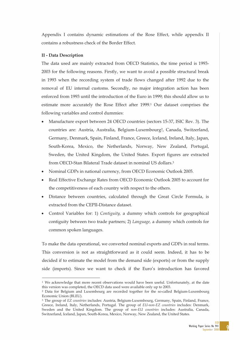
In Figure 1 we plot the yearly Overall Total Export among the OECD24 countries,

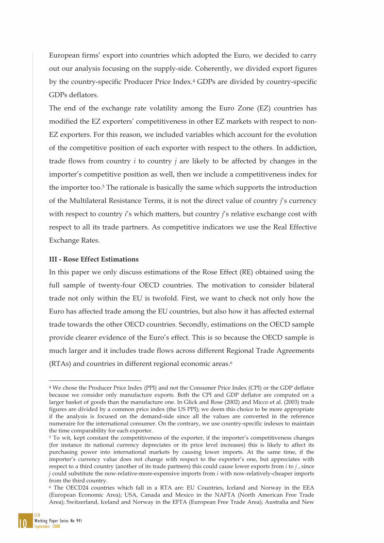
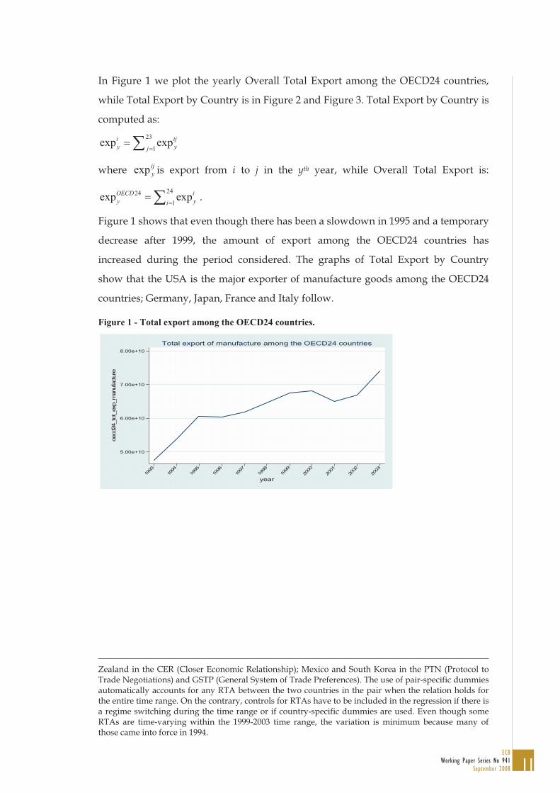
while Total Export by Country is in Figure 2 and Figure 3. Total Export by Country is

computed as:

23

1exp expi ij

y yj

where ij

yexp is export from i to j in the yth year, while Overall Total Export is:

2424

1exp expOECD i

y yi.

Figure 1 shows that even though there has been a slowdown in 1995 and a temporary

decrease after 1999, the amount of export among the OECD24 countries has

increased during the period considered. The graphs of Total Export by Country

show that the USA is the major exporter of manufacture goods among the OECD24

countries; Germany, Japan, France and Italy follow.

Figure 1 - Total export among the OECD24 countries.

5.00e+10

6.00e+10

7.00e+10

8.00e+10

oecd24_to

t_exp_m

anufa

ctu

re

1993

1994

1995

1996

1997

1998

1999

2000

2001

2002

2003

year

Total export of manufacture among the OECD24 countries

Zealand in the CER (Closer Economic Relationship); Mexico and South Korea in the PTN (Protocol to Trade Negotiations) and GSTP (General System of Trade Preferences). The use of pair-specific dummies automatically accounts for any RTA between the two countries in the pair when the relation holds for the entire time range. On the contrary, controls for RTAs have to be included in the regression if there is a regime switching during the time range or if country-specific dummies are used. Even though some RTAs are time-varying within the 1999-2003 time range, the variation is minimum because many of those came into force in 1994.


Figure 2 - Total Export by exporter.

0

2.00e+08

4.00e+08

6.00e+08

0

2.00e+08

4.00e+08

6.00e+08

0

2.00e+08

4.00e+08

6.00e+08

0

2.00e+08

4.00e+08

6.00e+08

199

3

199

4

199

5

199

6

199

7

199

8

199

9

200

0

200

1

200

2

200

3

199

3

199

4

199

5

199

6

199

7

199

8

199

9

200

0

200

1

200

2

200

3

199

3

199

4

199

5

199

6

199

7

199

8

199

9

200

0

200

1

200

2

200

3

AT AU BLEU

CA CH DE

DK ES FI

FR GR IC

tot_

exp

_m

anu

factu

re

yearGraphs by exporter

Exporter: Austria (AT), Australia (AU), Belgium Luxembourg (BLEU), Canada (CA), Switzerland (CH),

Germany (DE), Denmark (DK), Spain (ES), Finland (FI), France (FR), Greece (GR), Iceland (IC).

Figure 3 - Total Export by exporter.

0

2.00e+08

4.00e+08

6.00e+08

0

2.00e+08

4.00e+08

6.00e+08

0

2.00e+08

4.00e+08

6.00e+08

0

2.00e+08

4.00e+08

6.00e+08

199

3

199

4

199

5

199

6

199

7

199

8

199

9

200

0

200

1

200

2

200

3

199

3

199

4

199

5

199

6

199

7

199

8

199

9

200

0

200

1

200

2

200

3

199

3

199

4

199

5

199

6

199

7

199

8

199

9

200

0

200

1

200

2

200

3

IE IT JP

KO MX NL

NO NZ PT

SE UK US

tot_

exp

_m

anu

factu

re


Exporter: Ireland (IE), Italy (IT), Japan (JP), South Korea (KO), Mexico (MX), the Netherlands (NL),

Norway (NO), New Zealand (NZ), Portugal (PT), Sweden (SE), the United Kingdom (UK), the United

States (US).

13ECB


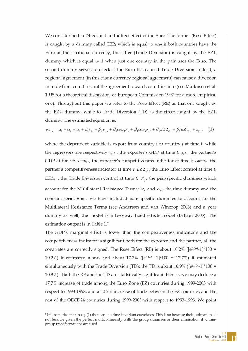
We consider both a Direct and an Indirect effect of the Euro. The former (Rose Effect)

is caught by a dummy called EZ2t which is equal to one if both countries have the

Euro as their national currency, the latter (Trade Diversion) is caught by the EZ1t

dummy which is equal to 1 when just one country in the pair uses the Euro. The

second dummy serves to check if the Euro has caused Trade Diversion. Indeed, a

regional agreement (in this case a currency regional agreement) can cause a diversion

in trade from countries out the agreement towards countries into (see Markusen et al.

1995 for a theoretical discussion, or European Commission 1997 for a more empirical

one). Throughout this paper we refer to the Rose Effect (RE) as that one caught by

the EZ2t dummy, while to Trade Diversion (TD) as the effect caught by the EZ1t

dummy. The estimated equation is:

, 0 1 , 2 , 3 , 4 , 5 , 6 , ,2 1

ij t ij t i t j t i t j t ij t ij t ij tex y y comp comp EZ EZ , (1)

where the dependent variable is export from country i to country j at time t, while

the regressors are respectively: yi,t , the exporter’s GDP at time t; yj,t , the partner’s

GDP at time t; compi,t , the exporter’s competitiveness indicator at time t; compjt , the

partner’s competitiveness indicator at time t; EZ2ij,t , the Euro Effect control at time t;

EZ1ij,t , the Trade Diversion control at time t; ij , the pair-specific dummies which

account for the Multilateral Resistance Terms; t and 0 , the time dummy and the

constant term. Since we have included pair–specific dummies to account for the

Multilateral Resistance Terms (see Anderson and van Wincoop 2003) and a year

dummy as well, the model is a two-way fixed effects model (Baltagi 2005). The

estimation output is in Table 1.7

The GDP’s marginal effect is lower than the competitiveness indicator’s and the

competitiveness indicator is significant both for the exporter and the partner, all the

covariates are correctly signed. The Rose Effect (RE) is about 10.2% ([e0.098-1]*100 =

10.2%) if estimated alone, and about 17.7% ([e0.163 -1]*100 = 17.7%) if estimated

simultaneously with the Trade Diversion (TD); the TD is about 10.9% ([e0.104-1]*100 =

10.9%). Both the RE and the TD are statistically significant. Hence, we may deduce a

17.7% increase of trade among the Euro Zone (EZ) countries during 1999-2003 with

respect to 1993-1998, and a 10.9% increase of trade between the EZ countries and the

rest of the OECD24 countries during 1999-2003 with respect to 1993-1998. We point

7 It is to notice that in eq. (1) there are no time-invariant covariates. This is so because their estimation is not feasible given the perfect multicollinearity with the group dummies or their elimination if within-group transformations are used.


out that these values of the RE are realistic and literature-consistent (see Flam and

Nostrom 2003, or Micco et al. 2003).

Table 1 – Estimation of the RE and TD.

(1) (2)

WGE s.e. WGE s.e.

LOG_GDP_EXP 0.548 (0.079)** 0.541 (0.078)**

LOG_GDP_PAR 0.259 (0.051)** 0.253 (0.051)**

LOG_REER_EXP 0.640 (0.101)** 0.608 (0.101)**

LOG_REER_PAR 0.728 (0.072)** 0.756 (0.072)**

EZ2_t 0.098 (0.011)** 0.163 (0.015)**

EZ1_t 0.104 (0.015)**

Observations 6069 6069

Groups 552 552

Ov. R squared 0.492 0.492Countries included: OECD24. Pair and Year dummies included

Robust standard errors in parentheses * significant at 5%; ** significant at 1%

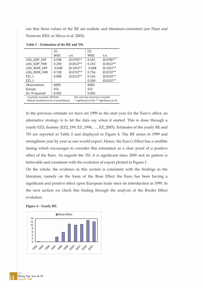
In the previous estimate we have set 1999 as the start year for the Euro’s effect, an

alternative strategy is to let the data say when it started. This is done through a

yearly EZ2t dummy (EZ2_199, EZ_1994, …, EZ_2003). Estimates of the yearly RE and

TD are reported in Table 2 and displayed in Figure 4. The RE arises in 1999 and

strengthens year by year as one would expect. Hence, the Euro’s Effect has a credible

timing which encourages to consider this estimation as a clear proof of a positive

effect of the Euro. As regards the TD, it is significant since 2000 and its pattern is

believable and consistent with the evolution of export plotted in Figure 1.

On the whole, the evidence in this section is consistent with the findings in the

literature, namely on the basis of the Rose Effect the Euro has been having a

significant and positive effect upon European trade since its introduction in 1999. In

the next section we check this finding through the analysis of the Border Effect

evolution.

Figure 4 - Yearly RE.

0

2

4

6

8

10

12

14

1994

1995

1996

1997

1998

1999

2000

2001

2002

2003

Rose Effect

15ECB


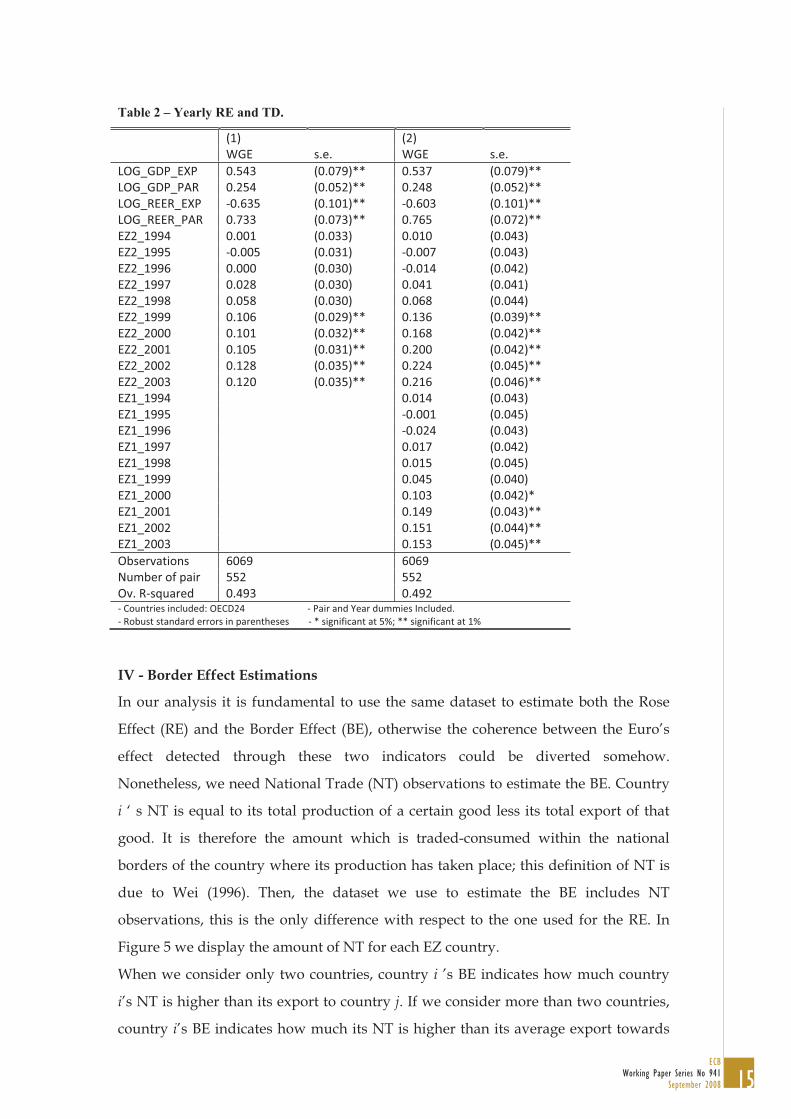
Table 2 – Yearly RE and TD.

(1) (2)

WGE s.e. WGE s.e.

LOG_GDP_EXP 0.543 (0.079)** 0.537 (0.079)**

LOG_GDP_PAR 0.254 (0.052)** 0.248 (0.052)**

LOG_REER_EXP 0.635 (0.101)** 0.603 (0.101)**

LOG_REER_PAR 0.733 (0.073)** 0.765 (0.072)**

EZ2_1994 0.001 (0.033) 0.010 (0.043)

EZ2_1995 0.005 (0.031) 0.007 (0.043)

EZ2_1996 0.000 (0.030) 0.014 (0.042)

EZ2_1997 0.028 (0.030) 0.041 (0.041)

EZ2_1998 0.058 (0.030) 0.068 (0.044)

EZ2_1999 0.106 (0.029)** 0.136 (0.039)**

EZ2_2000 0.101 (0.032)** 0.168 (0.042)**

EZ2_2001 0.105 (0.031)** 0.200 (0.042)**

EZ2_2002 0.128 (0.035)** 0.224 (0.045)**

EZ2_2003 0.120 (0.035)** 0.216 (0.046)**

EZ1_1994 0.014 (0.043)

EZ1_1995 0.001 (0.045)

EZ1_1996 0.024 (0.043)

EZ1_1997 0.017 (0.042)

EZ1_1998 0.015 (0.045)

EZ1_1999 0.045 (0.040)

EZ1_2000 0.103 (0.042)*

EZ1_2001 0.149 (0.043)**

EZ1_2002 0.151 (0.044)**

EZ1_2003 0.153 (0.045)**

Observations 6069 6069

Number of pair 552 552

Ov. R squared 0.493 0.492Countries included: OECD24 Pair and Year dummies Included.

Robust standard errors in parentheses * significant at 5%; ** significant at 1%

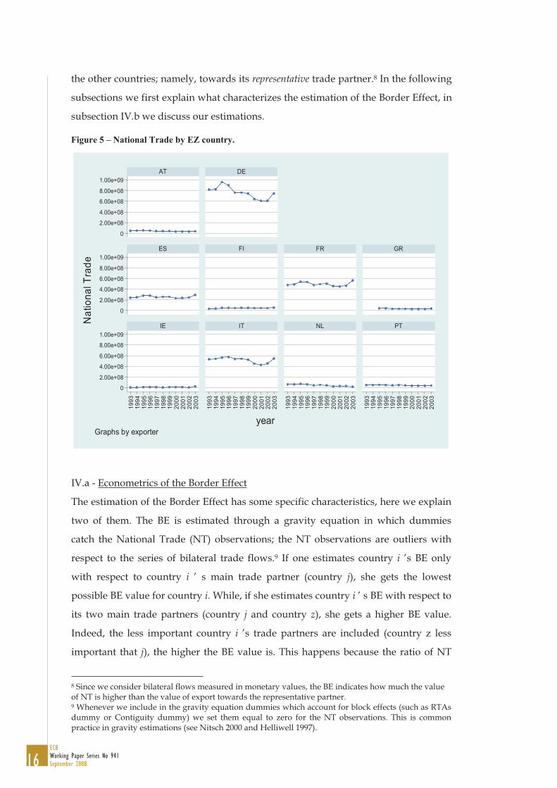
In our analysis it is fundamental to use the same dataset to estimate both the Rose

Effect (RE) and the Border Effect (BE), otherwise the coherence between the Euro’s

effect detected through these two indicators could be diverted somehow.

Nonetheless, we need National Trade (NT) observations to estimate the BE. Country

i ‘ s NT is equal to its total production of a certain good less its total export of that

good. It is therefore the amount which is traded-consumed within the national

borders of the country where its production has taken place; this definition of NT is

due to Wei (1996). Then, the dataset we use to estimate the BE includes NT

observations, this is the only difference with respect to the one used for the RE. In

Figure 5 we display the amount of NT for each EZ country.

When we consider only two countries, country i ’s BE indicates how much country

i’s NT is higher than its export to country j. If we consider more than two countries,

country i’s BE indicates how much its NT is higher than its average export towards

IV - Border Effect Estimations


the other countries; namely, towards its representative trade partner.8 In the following

subsections we first explain what characterizes the estimation of the Border Effect, in

subsection IV.b we discuss our estimations.

Figure 5 – National Trade by EZ country.

0

2.00e+08

4.00e+08

6.00e+08

8.00e+08

1.00e+09

0

2.00e+08

4.00e+08

6.00e+08

8.00e+08

1.00e+09

0

2.00e+08

4.00e+08

6.00e+08

8.00e+08

1.00e+09

19

93

19

94

19

95

19

96

19

97

19

98

19

99

20

00

20

01

20

02

20

03

19

93

19

94

19

95

19

96

19

97

19

98

19

99

20

00

20

01

20

02

20

03

19

93

19

94

19

95

19

96

19

97

19

98

19

99

20

00

20

01

20

02

20

03

19

93

19

94

19

95

19

96

19

97

19

98

19

99

20

00

20

01

20

02

20

03

AT DE

ES FI FR GR

IE IT NL PT

Na

tio

na

l T

rad

e


The estimation of the Border Effect has some specific characteristics, here we explain

two of them. The BE is estimated through a gravity equation in which dummies

catch the National Trade (NT) observations; the NT observations are outliers with

respect to the series of bilateral trade flows.9 If one estimates country i ’s BE only

with respect to country i ’ s main trade partner (country j), she gets the lowest

possible BE value for country i. While, if she estimates country i ’ s BE with respect to

its two main trade partners (country j and country z), she gets a higher BE value.

Indeed, the less important country i ’s trade partners are included (country z less

important that j), the higher the BE value is. This happens because the ratio of NT

8 Since we consider bilateral flows measured in monetary values, the BE indicates how much the value of NT is higher than the value of export towards the representative partner. 9 Whenever we include in the gravity equation dummies which account for block effects (such as RTAs dummy or Contiguity dummy) we set them equal to zero for the NT observations. This is common practice in gravity estimations (see Nitsch 2000 and Helliwell 1997).

IV.a - Econometrics of the Border Effect

17ECB


over export towards the representative partner increases. Hence, any EU country’s

BE with respect to the group of its EU partners is lower than its BE with respect to a

larger sample of trade partners (the EU sample is nested in the larger) because the

EU as a whole is the main trade partner of any European country (see Eurostat 2003).

For this reason, when we want to estimate the BE, we have to include only the

countries in which we are interested; we therefore included only the EU countries in

the BE estimations.

Another important characteristic of the BE estimation is that we cannot use pair-

specific dummies to proxy the Multilateral Resistance Terms. Indeed, if we do so, the

NT observations will be caught by two different dummies and the BE cannot be

estimated. Hence, after many attempts, we eventually concluded that for the

objective of this paper (and probably whenever researchers are interested in the

evolution of the BE) pair-specific dummies are not suitable to model the Multilateral

Resistance Terms.10

We now discuss the estimation of the gravity equation which provides us with an

estimate of the Border Effect (BE). In this gravity equation the Multilateral Resistance

Terms are modelled through Country-Specific Time-Invariant dummies. To infer the

effect of the Euro through the evolution of the BE, we study the BE on a sample of

data which includes only the European countries for the reason abovementioned.

Then, the average BE ex-ante and ex-post 1999, both for the Euro Zone (EZ) countries

and for Denmark, Sweden and the UK (EU non EZ countries), is estimated through

the following equation:

, 0 1 , 2 , 3 , 4 , 5 6

NT_EZ_ante99 NT_EZ_post99 NT_EUnoEZ_ante99 NT_EUnoEZ_post997 8 9 10 11 ,

ij t i j t i t j t i t j t ij ij

ij ij t

ex y y comp comp dist contig

lang (2)

The dependent variable exij,t is export from country i to country j at time t. The

covariates are respectively: yi,t , the exporter’s GDP at time t; yj,t , the partner’s GDP at

time t; compi,t , exporter’s competitiveness indicator at time t; compj,t , partner’s

competitiveness indicator at time t; distij , distance between country i and j; contigij ,

10 For the same reason the estimation of the BE in a dynamic panel framework seems not to be econometrically feasible. In fact, to perform dynamic panel regressions it is necessary to define the group indicator on which to calculate the first difference of the equation (GMM procedures) or to include group dummies (Least Squares Dummy Variables Corrected). But, as explained, we cannot estimate the BE whenever a pair-dummy is included in the regression or the pair is taken as group indicator.

IV.b - Estimations of the Border Effect


Contiguity control; langij , Common Language control; NTij_..., National Trade

dummies.11

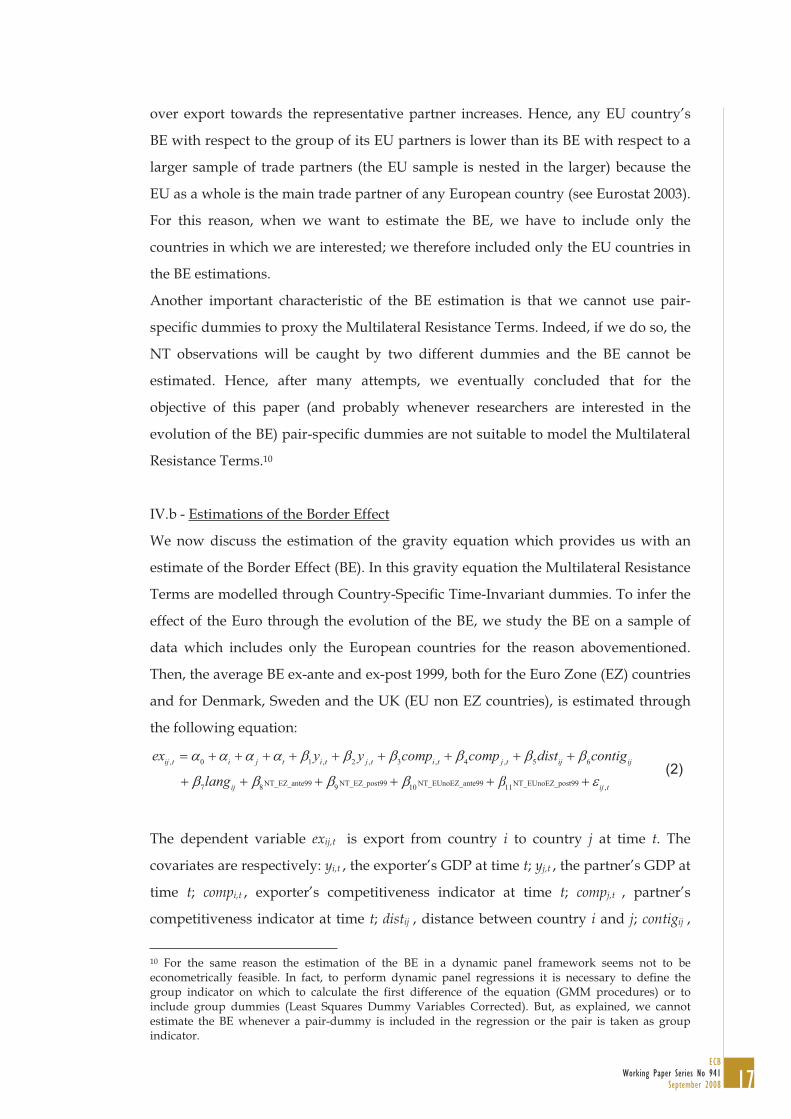
The regression output is in Table 3, while the histogram of the estimated BEs is in

Figure 6. The BE reduction between 1993-1998 and 1999-2003 is about 23.6% ([e2.22 -

e2.49]/e2.49) for the EZ countries and 26.6% for the EU-non-EZ countries ([e1.80-

e2.11]/e2.11). Hence, the percentage decrease is larger for the EU-non-EZ countries,

while we expected a stronger BE decrease for the EZ countries in case of a positive

and relevant effect of the Euro. This first evidence against a significant Euro’s effect is

strengthened by the results of the Wald test of linear restrictions. The linear

restriction “EZ countries’ BE equal before and after 1999” is not rejected (p-value

0.104), while the hypothesis “EU-non-EZ countries’ BE equal before and after 1999”

is rejected (p-value 0.002); both the hypothesis “EZ countries’ BE equal to EU-non-EZ

countries’ before 1999” and “EZ countries’ BE equal to EU-non-EZ countries’ after

1999” are rejected (p-value 0.001 and 0.004).

Table 3 - BE by group and time interval.

LSDV s.e.

LOG_GDP_EXP 0.914 (0.173)**

LOG_GDP_PAR 0.661 (0.158)**

LOG_REER_EXP 0.864 (0.229)**

LOG_REER_PAR 0.009 (0.210)

LOG_DISTANCE 0.776 (0.030)**

CONTIGUITY 0.367 (0.036)**

LANGUAGE 0.329 (0.061)**

B_eu_ez_post99 2.229 (0.144)**

b_eu_ez_ante99 2.491 (0.116)**

b_eu_noez_post99 1.809 (0.092)**

b_eu_noez_ante99 2.116 (0.085)**

Observations 2143

Deg.ofFree. 2095

R squared 0.95Countries included: EU14

Exporter and Partner plus Year dummies included

Robust standard errors in parentheses

* Significant at 5%, ** significant at 1%

Figure 6 - BE by group and time interval.

BORDER

0

2

4

6

8

10

12

14

1993-1998 1999-2003

tim

es h

igh

er

than

ext.

tra

de

EU_EZ EU_NOEZ

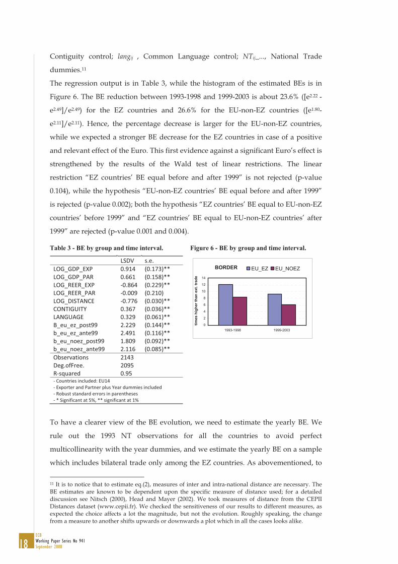
To have a clearer view of the BE evolution, we need to estimate the yearly BE. We

rule out the 1993 NT observations for all the countries to avoid perfect

multicollinearity with the year dummies, and we estimate the yearly BE on a sample

which includes bilateral trade only among the EZ countries. As abovementioned, to

11 It is to notice that to estimate eq.(2), measures of inter and intra-national distance are necessary. The BE estimates are known to be dependent upon the specific measure of distance used; for a detailed discussion see Nitsch (2000), Head and Mayer (2002). We took measures of distance from the CEPII Distances dataset (www.cepii.fr). We checked the sensitiveness of our results to different measures, as expected the choice affects a lot the magnitude, but not the evolution. Roughly speaking, the change from a measure to another shifts upwards or downwards a plot which in all the cases looks alike.

19ECB


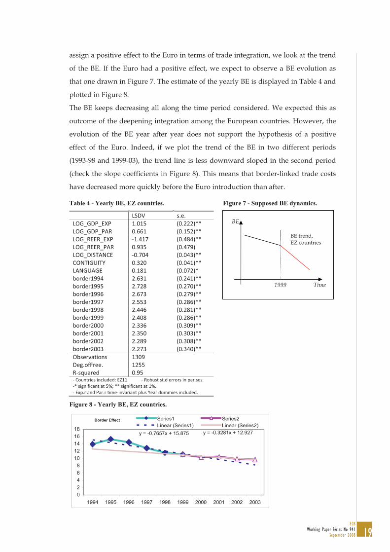
assign a positive effect to the Euro in terms of trade integration, we look at the trend

of the BE. If the Euro had a positive effect, we expect to observe a BE evolution as

that one drawn in Figure 7. The estimate of the yearly BE is displayed in Table 4 and

plotted in Figure 8.

The BE keeps decreasing all along the time period considered. We expected this as

outcome of the deepening integration among the European countries. However, the

evolution of the BE year after year does not support the hypothesis of a positive

effect of the Euro. Indeed, if we plot the trend of the BE in two different periods

(1993-98 and 1999-03), the trend line is less downward sloped in the second period

(check the slope coefficients in Figure 8). This means that border-linked trade costs

have decreased more quickly before the Euro introduction than after.

Table 4 - Yearly BE, EZ countries.

LSDV s.e.

LOG_GDP_EXP 1.015 (0.222)**

LOG_GDP_PAR 0.661 (0.152)**

LOG_REER_EXP 1.417 (0.484)**

LOG_REER_PAR 0.935 (0.479)

LOG_DISTANCE 0.704 (0.043)**

CONTIGUITY 0.320 (0.041)**

LANGUAGE 0.181 (0.072)*

border1994 2.631 (0.241)**

border1995 2.728 (0.270)**

border1996 2.673 (0.279)**

border1997 2.553 (0.286)**

border1998 2.446 (0.281)**

border1999 2.408 (0.286)**

border2000 2.336 (0.309)**

border2001 2.350 (0.303)**

border2002 2.289 (0.308)**

border2003 2.273 (0.340)**

Observations 1309

Deg.ofFree. 1255

R squared 0.95Countries included: EZ11. Robust st.d errors in par.ses.

* significant at 5%; ** significant at 1%.

Exp.r and Par.r time invariant plus Year dummies included.

Figure 7 - Supposed BE dynamics.

Figure 8 - Yearly BE, EZ countries.

Border Effect

y = -0.7657x + 15.875 y = -0.3281x + 12.927

0

2

4

6

8

10

12

14

16

18

1994 1995 1996 1997 1998 1999 2000 2001 2002 2003

Series1 Series2

Linear (Series1) Linear (Series2)

Time

BE

1999

BE trend, EZ countries


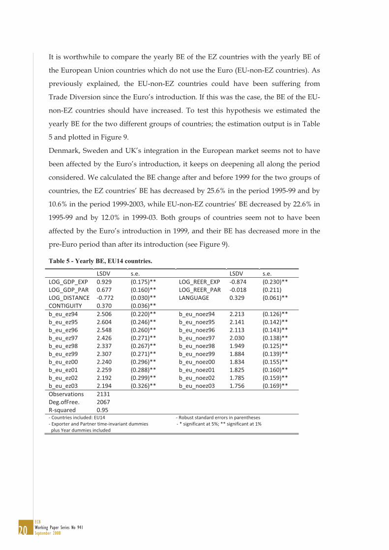
It is worthwhile to compare the yearly BE of the EZ countries with the yearly BE of

the European Union countries which do not use the Euro (EU-non-EZ countries). As

previously explained, the EU-non-EZ countries could have been suffering from

Trade Diversion since the Euro’s introduction. If this was the case, the BE of the EU-

non-EZ countries should have increased. To test this hypothesis we estimated the

yearly BE for the two different groups of countries; the estimation output is in Table

5 and plotted in Figure 9.

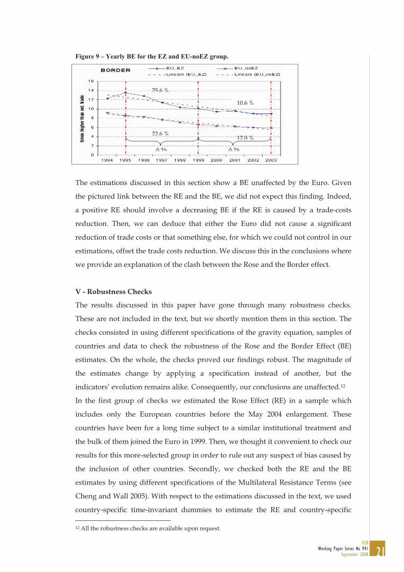
Denmark, Sweden and UK’s integration in the European market seems not to have

been affected by the Euro’s introduction, it keeps on deepening all along the period

considered. We calculated the BE change after and before 1999 for the two groups of

countries, the EZ countries’ BE has decreased by 25.6% in the period 1995-99 and by

10.6% in the period 1999-2003, while EU-non-EZ countries’ BE decreased by 22.6% in

1995-99 and by 12.0% in 1999-03. Both groups of countries seem not to have been

affected by the Euro’s introduction in 1999, and their BE has decreased more in the

pre-Euro period than after its introduction (see Figure 9).

Table 5 - Yearly BE, EU14 countries.

LSDV s.e. LSDV s.e.

LOG_GDP_EXP 0.929 (0.175)** LOG_REER_EXP 0.874 (0.230)**

LOG_GDP_PAR 0.677 (0.160)** LOG_REER_PAR 0.018 (0.211)

LOG_DISTANCE 0.772 (0.030)** LANGUAGE 0.329 (0.061)**

CONTIGUITY 0.370 (0.036)**

b_eu_ez94 2.506 (0.220)** b_eu_noez94 2.213 (0.126)**

b_eu_ez95 2.604 (0.246)** b_eu_noez95 2.141 (0.142)**

b_eu_ez96 2.548 (0.260)** b_eu_noez96 2.113 (0.143)**

b_eu_ez97 2.426 (0.271)** b_eu_noez97 2.030 (0.138)**

b_eu_ez98 2.337 (0.267)** b_eu_noez98 1.949 (0.125)**

b_eu_ez99 2.307 (0.271)** b_eu_noez99 1.884 (0.139)**

b_eu_ez00 2.240 (0.296)** b_eu_noez00 1.834 (0.155)**

b_eu_ez01 2.259 (0.288)** b_eu_noez01 1.825 (0.160)**

b_eu_ez02 2.192 (0.299)** b_eu_noez02 1.785 (0.159)**

b_eu_ez03 2.194 (0.326)** b_eu_noez03 1.756 (0.169)**

Observations 2131

Deg.ofFree. 2067

R squared 0.95Countries included: EU14 Robust standard errors in parentheses

Exporter and Partner time invariant dummies * significant at 5%; ** significant at 1%

plus Year dummies included

21ECB


Figure 9 – Yearly BE for the EZ and EU-noEZ group.

The estimations discussed in this section show a BE unaffected by the Euro. Given

the pictured link between the RE and the BE, we did not expect this finding. Indeed,

a positive RE should involve a decreasing BE if the RE is caused by a trade-costs

reduction. Then, we can deduce that either the Euro did not cause a significant

reduction of trade costs or that something else, for which we could not control in our

estimations, offset the trade costs reduction. We discuss this in the conclusions where

we provide an explanation of the clash between the Rose and the Border effect.

The results discussed in this paper have gone through many robustness checks.

These are not included in the text, but we shortly mention them in this section. The

checks consisted in using different specifications of the gravity equation, samples of

countries and data to check the robustness of the Rose and the Border Effect (BE)

estimates. On the whole, the checks proved our findings robust. The magnitude of

the estimates change by applying a specification instead of another, but the

indicators’ evolution remains alike. Consequently, our conclusions are unaffected.12

In the first group of checks we estimated the Rose Effect (RE) in a sample which

includes only the European countries before the May 2004 enlargement. These

countries have been for a long time subject to a similar institutional treatment and

the bulk of them joined the Euro in 1999. Then, we thought it convenient to check our

results for this more-selected group in order to rule out any suspect of bias caused by

the inclusion of other countries. Secondly, we checked both the RE and the BE

estimates by using different specifications of the Multilateral Resistance Terms (see

Cheng and Wall 2005). With respect to the estimations discussed in the text, we used

country-specific time-invariant dummies to estimate the RE and country-specific

12 All the robustness checks are available upon request.

12.0 %

25.6 %

10.6 %

22.6 %

V - Robustness Checks


time-varying dummies (as suggested by Baldwin 2006) to estimate the BE. We

thought this to be an important check. Indeed, there is not consensus about the right

specification of the gravity equation and on how to account for factors that cannot be

caught by any specific control.

Thirdly, we used a large sectoral dataset to check both the RE and the BE sector by

sector. This was done to get sure that the results discussed in the paper are not

dependent upon aggregation and not limited to aggregate analyses. For the majority

of the sectors considered, the sectoral RE and BE have a similar pattern to the RE and

BE estimated using aggregate data. Hence, sectoral and aggregate estimations are

unanimous about the pattern of the RE and BE in the period considered. Forth, we

used different measures of distance to find out how much the BE estimates are

sensitive to any specific one. As mentioned in footnote 11, the change from one

measure to another shifts upwards or downwards a plot which in all the cases looks

alike.

We have dedicated the two appendices of this paper to the discussion of some other

robustness checks which we deemed of greater interest. Appendix I contains

dynamic estimations of the RE, while in Appendix II we discuss an intuitive check of

the yearly BE estimate in Table 4. We refer the reader to those appendices for a

detailed discussion.

Our main finding is that, on the basis of the Rose Effect, the Euro has influenced

European trade after 1999, while there is no effect of the Euro according to the

evolution of the Border Effect. The most-quoted theoretical explanation of the Rose

Effect is founded on the removal of border-linked costs (this is one of the main

argument of the Optimum Currency Area literature, see Baldwin and Wyplosz 2004),

but we deem the Border Effect to be the true indicator of border-linked costs. Then,

given the evolution of the estimated Border Effect, we are prone to believe that there

was no acceleration in the reduction of border-linked costs (with respect to the

historical tendency) after the Euro’s introduction. Consequently, we can either

believe that the Rose Effect does not catch the effect of the Euro (it is a spurious

outcome) or that the effect of the Euro caught by the Rose Effect is due to something

else than a reduction in border-linked trade costs.

Let us begin considering the first option. Berger and Nitsch (2005) and Mongelli et al.

(2005) show that economic integration was rising steeply just before Euro’s

VI - Conclusions

23ECB


introduction. Their thesis is that pro-trade adjustments to pre-Euro integration take

time, then it could be that the lagged effects of Single Market measures show up in

the post-1999 data and get blurred with the trade effects of the Euro. This would not

be a problem for Rose Effect estimations if only all EU members introduced Single

Market measures at the same time, but EU members differ widely on their pace of

implementing EU directives.13 Even though we have used a dynamic specification of

the gravity equation and controlled for common shocks -through the year dummies-

and country-specific shocks, one can not be completely sure that this catches

everything but the effect of the Euro. Indeed, it may be quite difficult to effectively

disentangle the effects of European integration from the Euro’s because European

integration is a work in progress as the Border Effect evolution shows (as well as

Berger and Nitsch 2005, and Mongelli et al. 2005). Then, there is a chance that the

Euro’s effect detected is nothing more than the delayed and differential effect of pro-

trade directives as the BE evolution suggests.

On the contrary, if we believe that the Rose Effect correctly catches the increase in

exchanges due to the Euro’s introduction, the question to answer is what else than a

trade costs reduction could have caused such increase. Answers founded on output

variations or changes in the cross-countries competitive position are not believable

since we controlled for those. In our estimations, we found that trade between the EZ

countries and other nations rose with the Euro’s introduction, but not as much as

trade among the EZ countries (see Table 2 and 3). This result is intriguing and tends

to reject the cost-reduction explanation of the Rose Effect because in that case there

should have been trade diversion. The Euro would have been akin to a

discriminatory liberalisation and this should have reduced the exports of non-Euro

nations to the Euro Zone as Baldwin (2006) suggests. According to Baldwin (2006),

an explanation of the positive Rose Effect not founded on costs reduction and not

conflicting with trade creation can be found in Baldwin and Taglioni (2004). Their

basic intuition is simple. Most European firms were not engaged in trade before the

Euro’s introduction, they sold only in their local markets due to a variety of reasons,

one of which is aversion to exchange rate uncertainty. Such uncertainty is easily

faced by large companies but to small and medium firms it is as a real barrier. Since

monetary unions eliminate this uncertainty, the number of EZ firms engaged in

export to other EZ markets increased after the Euro’s introduction. Consequently, we

13 The Internal Market Scoreboard gives an account of the difference in implementing EU directives among the EU countries. More information and the Scoreboard itself can be found at “http://ec.europa.eu/internal_market/score/index_en.htm”


observe a trade-flows increase after 1999. Furthermore, more transparency and

cost/price comparability as well as higher ease to access other national markets after

the Euro’s introduction could have worked in the same manner as the removal of

exchange rate uncertainty just discussed.

On the whole, we are prone to believe that the Rose Effect is not a spurious outcome

because it emerges in many papers which use different econometric techniques,

datasets and time intervals, and because it is always clearly detected in 1999. It is

unlikely that all of us made the same mistake and that it emerges always around

1999 by chance. Consequently, we deem more likely the second case just discussed.

Namely, the Rose Effect catches an increase in exchanges linked to the Euro’s

introduction, but that increase can not be explained through an acceleration in the

reduction of border-linked trade costs among the countries which adopted the Euro.

25ECB


Appendix I - Dynamic Estimations of the Rose Effects.

Trade flows are observed to be persistent over time. There are different explanations

for this, one is habit formation in consumption and another is based on

internationalization and sunk costs linked to export in a foreign market (Evans 2003,

Eichengreen and Irwin 1997). Then, we could need to include lagged values of the

dependent variable to write the model in a correct econometric way (Bun and

Klassen 2002). In this section we discuss dynamic estimations of the RE obtained

through two different estimators, these serve as robustness checks of the static ones

in section III. The first estimator used is a General Method of Moments (GMM)

estimator, the second is the Least Squares Dummy Variables Corrected estimator; we

start with the GMM estimator.14

In the group of GMM estimators available, we chose the Arellano-Bond estimator

because of the low coefficient of the lagged dependent variable.15 The model which

we estimate is:

tijtjtitjtitijtijtij compcompyyexex ,,4,3,2,11,00, . (3)

In any Arellano-Bond estimation there is need to define the Instruments Matrix. This

matrix includes the lagged levels of the dependent variable by default, the researcher

can also include as additional instruments the regressors in the equation to estimate.

However, these can be included only if they are strictly exogenous or predetermined

(a regressor x is Predetermined when 0][ ,, siti vxE for t < s, t and s = 1…T; Strictly

Exogenous when 0][ ,, siti vxE for t and s). The definition of each regressor as

strictly exogenous, predetermined or excluded instrument should be based on the

Difference Sargan Test (DST) and the economic nature of the variable itself.16

Unfortunately, the DST is not always reliable (rejects too often) when the data are

affected by heteroskedasticity as argued by Arellano and Bond (1991).17 For this

14 Given the longitudinal and time dimension of our panel, GMM estimators are probably the most suitable, see Judson and Owen (1999) for a discussion about the choice of the dynamic estimator.15 An alternative is the Blundel-Bond estimator more suited in case of a high coefficient of the lagged Dependent Variable (see Bond 2002). 16 The DST checks the validity of the additional over-identifying restrictions due to shifting from a model with less to a model with more restrictions (namely, more instruments included).17 According to the DST, we should have included in the Instruments Matrix either the Competitiveness indicators or the GDPs variables as predetermined, or both as strictly exogenous. Only when we impose a very small number of restrictions (around 60) the Sargan (1958) test (and not the Difference Sargan Test) does not reject the hypothesis of valid instruments (see Bond 2002 for an example of instruments selection by means of the DST). Though, the estimated coefficients are not gravity-consistent if those settings are used.


reason, we did not follow the conclusions of the DST, instead we defined the

regressors according to a reasonable economic rationale. Consequently we thought to

have two possible settings: a) past values of the competitiveness indicators and of the

GDPs do not influence current bilateral exports, in this case both variables are

predetermined and their past values can be included in the Instruments Matrix; b)

only past values of the competitiveness indicators do not influence current bilateral

exports, while GDP is endogenous and it has to be left out.

We run estimations for both settings, in either the Arellano-Bond test for second

order autocorrelation rejects the null, so we did not doubt the consistency of the

Arellano-Bond estimator. We performed both ONE-Step and TWO-Step GMM

estimations (see Arellano 2003, appendix A.7). We point out that the TWO-Step

standard errors are computed in accordance to the Windmeijer finite-sample

correction (otherwise they are seriously biased, see Windmeijer 2005).18

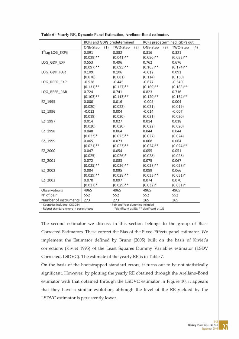
The estimate of the yearly RE is in Table 6. We choose regression 2 as our preferred

for the following reasons. First, the estimation of regression 1 and 2 is more efficient

than that of regression 3 and 4 because the GMM estimator increases its efficiency

when more restrictions are imposed (in regression 1 and 2 the Instruments-Matrix

includes two more instruments). Second, since the TWO-Step robust estimation is

more efficient than the ONE-Step robust, we prefer regression 2 to regression 1. We

acknowledge that defining the GDP as predetermined is questionable, however the

results are not driven by this choice. Indeed, the coefficients are slightly different

across estimates.

On the basis of the estimation output, the RE arises in 1998 and not in 1999 as it was

in the static regressions in section III (compare Table 6 with Table 2). From a cross-

regressions comparison, it turns out that the RE is present and strongly significant in

1999, it weakens in 2000 but it strengthens again in 2001.

18 The Two-Step procedure allows computing the optimal Weights-Matrix of the GMM estimator (see Hansen 1982) on the basis of the consistent estimate run at the first step. Nonetheless, this estimate at the second step is not efficient in case of heteroskedasticity. Then, it is common practice to apply the Windmeijer (2005) correction.

27ECB


Table 6 - Yearly RE, Dynamic Panel Estimation, Arellano-Bond estimator.

RCPs and GDPs predetermined RCPs predetermined, GDPs out

ONE Step (1) TWO Step (2) ONE Step (3) TWO Step (4)

1stlag LOG_EXPij 0.391 0.382 0.316 0.321

(0.039)** (0.041)** (0.050)** (0.052)**

LOG_GDP_EXP 0.553 0.496 0.762 0.676

(0.097)** (0.095)** (0.165)** (0.174)**

LOG_GDP_PAR 0.109 0.106 0.012 0.091

(0.078) (0.081) (0.114) (0.130)

LOG_REER_EXP 0.528 0.445 0.677 0.540

(0.131)** (0.127)** (0.169)** (0.183)**

LOG_REER_PAR 0.724 0.741 0.823 0.716

(0.103)** (0.113)** (0.120)** (0.154)**

EZ_1995 0.000 0.016 0.005 0.004

(0.020) (0.022) (0.021) (0.019)

EZ_1996 0.012 0.004 0.014 0.007

(0.019) (0.020) (0.021) (0.020)

EZ_1997 0.014 0.027 0.014 0.018

(0.020) (0.020) (0.022) (0.020)

EZ_1998 0.048 0.064 0.044 0.044

(0.023)* (0.023)** (0.027) (0.024)

EZ_1999 0.065 0.073 0.068 0.064

(0.021)** (0.023)** (0.024)** (0.024)**

EZ_2000 0.047 0.054 0.055 0.051

(0.025) (0.026)* (0.028) (0.028)

EZ_2001 0.072 0.083 0.075 0.067

(0.025)** (0.026)** (0.028)** (0.028)*

EZ_2002 0.084 0.095 0.089 0.066

(0.029)** (0.028)** (0.033)** (0.031)*

EZ_2003 0.070 0.097 0.074 0.070

(0.027)* (0.029)** (0.032)* (0.031)*

Observations 4965 4965 4965 4965

N° of pair 552 552 552 552

Number of instruments 273 273 165 165Countries included: OECD24 Pair and Year dummies included

Robust standard errors in parentheses *significant at 5%; ** significant at 1%

The second estimator we discuss in this section belongs to the group of Bias-

Corrected Estimators. These correct the Bias of the Fixed-Effects panel estimator. We

implement the Estimator defined by Bruno (2005) built on the basis of Kiviet’s

corrections (Kiviet 1995) of the Least Squares Dummy Variables estimator (LSDV

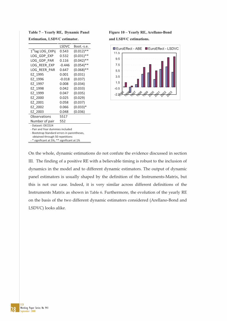
Corrected, LSDVC). The estimate of the yearly RE is in Table 7.

On the basis of the bootstrapped standard errors, it turns out to be not statistically

significant. However, by plotting the yearly RE obtained through the Arellano-Bond

estimator with that obtained through the LSDVC estimator in Figure 10, it appears

that they have a similar evolution, although the level of the RE yielded by the

LSDVC estimator is persistently lower.


Table 7 – Yearly RE, Dynamic Panel

Estimation, LSDVC estimator.

LSDVC Boot. s.e.

1stlag LOG_EXPij 0.543 (0.012)**

LOG_GDP_EXP 0.532 (0.031)**

LOG_GDP_PAR 0.116 (0.042)**

LOG_REER_EXP 0.446 (0.054)**

LOG_REER_PAR 0.647 (0.068)**

EZ_1995 0.001 (0.031)

EZ_1996 0.018 (0.037)

EZ_1997 0.008 (0.034)

EZ_1998 0.042 (0.033)

EZ_1999 0.047 (0.035)

EZ_2000 0.025 (0.029)

EZ_2001 0.058 (0.037)

EZ_2002 0.066 (0.033)*

EZ_2003 0.048 (0.036)

Observations 5517

Number of pair 552Dataset: OECD24

Pair and Year dummies included

Bootstrap Standard errors in parentheses,

obtained through 50 repetitions

* significant at 5%; ** significant at 1%

Figure 10 – Yearly RE, Arellano-Bond

and LSDVC estimations.

-2.5

-0.5

1.5

3.5

5.5

7.5

9.5

11.5

1995

1996

1997

1998

1999

2000

2001

2002

2003

EuroEffect - ABE EuroEffect - LSDVC

On the whole, dynamic estimations do not confute the evidence discussed in section

III. The finding of a positive RE with a believable timing is robust to the inclusion of

dynamics in the model and to different dynamic estimators. The output of dynamic

panel estimators is usually shaped by the definition of the Instruments-Matrix, but

this is not our case. Indeed, it is very similar across different definitions of the

Instruments Matrix as shown in Table 6. Furthermore, the evolution of the yearly RE

on the basis of the two different dynamic estimators considered (Arellano-Bond and

LSDVC) looks alike.

29ECB


Appendix II - An alternative check of the Border Effect.

The Border Effect estimated in a gravity equation is exposed to the bias typical of an

econometric regression. For this reason it is worthwhile to think to a possible

robustness check of the Border Effect (BE). With this purpose we can compute a ratio

whose evolution over time can be compared to the BE’s. It is the ratio of National

Trade (NT) over average export. In this section we compute this ratio for the group

of EZ countries.

To compute the ratio we need to proceed in two steps. First, we define a Country-

specific Border Ratio, and then an Aggregate Border Ratio; the former is nested in the

latter. Country i‘s Border Ratio is equal to its NT over its average export towards the

group of its trade partners:

1/

yy ii n y

ijj

NTCBR

ex n, (4)

where: i is the exporter (i = 1,…, n), j is the partner (j = 1,…, n), y is the year (y = 1,…,

m), y

iNT is country i ’s NT during the yth year and y

ijex is export from i to j during the

yth year. Since we consider only the Euro Zone (EZ) countries, n and m are equal to

11. To compute the same ratio but for the EZ countries altogether, the formula

becomes:

10 10

1 1

10 10 11

1 1 1

y y

i iy i i

y yi iji i j

NT NTABR

ex ex, (5)

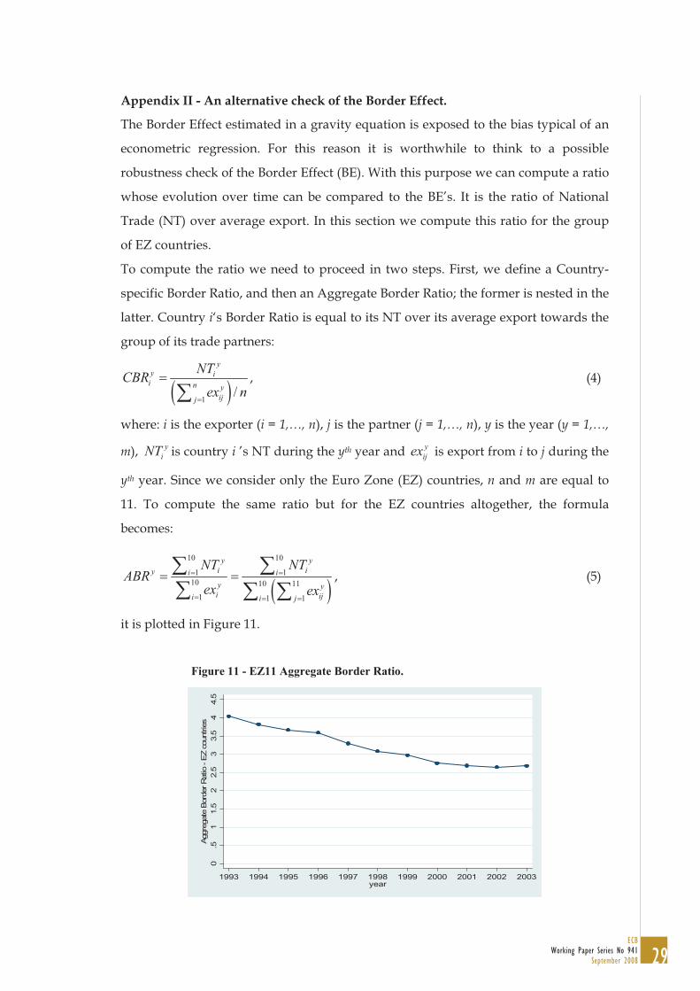
it is plotted in Figure 11.

Figure 11 - EZ11 Aggregate Border Ratio.

0.5

11.5

22.5

33.5

44.5

Aggre

gate

Bord

er R

atio - E

Z c

ountrie

s

1993 1994 1995 1996 1997 1998 1999 2000 2001 2002 2003year


A decrease of the ratio plotted in Figure 11 indicates that NT has decreased with

respect to average export, this suggests that nationals are less oriented towards home

consumption. This rationale suits a decrease of the Border Effect (BE) as well, then

the Border Ratio can serve as a robustness check of the BE estimation. In our analysis,

it confirms the evolution of the BE as it emerges from the estimation in Table 4 and

the plot in Figure 8.

31ECB


Bibliographical References

Anderson J. E. and E. van Wincoop (2003), “Gravity with Gravitas: A Solution to the Border Puzzle”, American Economic Review, 93(1): 170-192.

Anderson J. E. and E. van Wincoop (2004), “Trade Costs”, Journal of Economic Literature, 42(3): 691-751.

Arellano M. (2003), Panel Data Econometrics, Oxford University Press.

Arellano M. and S. Bond (1991),”Some tests of Specification for Panel Data: Monte Carlo Evidence and an application to Employment Equations”, Review of Economic Studies, 58(2).

Baldwin R. (2006), “Euro’s trade effects”, ECB Working Paper, n° 594.

Baldwin R. and D. Taglioni, (2004), “Positive OCA criteria: Microfoundations for the Rose effect,” Graduate Institute of International Studies, mimeo.

Baldwin R. and C. Wyplosz (2004), The Economics of European Integration, McGraw-Hill.

Baltagi B. H. (2005), Econometric Analysis of Panel Data, John Wiley & Sons.

Berger H. and V. Nitsch (2005), “Zooming Out: The Trade Effect of the Euro in Historical Perspective”, CESifo working paper, n° 1435.

Bond S. (2002), “Dynamic Panel Data Models: A guide to Micro Data Methods and Practice”, CEMMAP Working Paper, CWP09/02.

Bruno G. (2005), “Estimation and Inference in Dynamic Unbalanced Panel Data Models with a Small Number of Individual”, CESPRI Working Paper, n° 165.

Bun M. J. G. and F. J. G. M. Klaassen (2002), “The Importance of Dynamics in Panel Gravity Models of Trade”, UvA Econometrics, Discussion Paper 2002/18.

Chen N. (2004), “Intra-national versus international trade in the European Union: Why do National Borders matter?”, Journal of International Economics 63: 93-118.

Cheng I-Hui and H. Wall (2005), “Controlling for Heterogeneity in Gravity Models of Trade and Integration”, Federal Reserve Bank of St. Louis Review , 87(1): 49-63.

Eichengreen B. and D. Irwin (1997), “The role of history in bilateral trade flows”, in: The Regionalization of the World Economy, Frankel J., ed., University of Chicago Press, 33-57.

Emerson M. D., A. Italanier, J. Pisani-Ferry and H. Reichenbach (1992), One Market, One Money: An Evaluation of the Potential Benefits and Costs of Forming an Economic and Monetary Union, Oxford University Press.

Engel C. and J. H. Rogers (1996), “How Wide Is the Border ?”, American Economic Review, 86(5): 1112-25.


Eurostat (2003), Panorama of European Union Trade, Statistical Agency of the European Commission, Luxembourg.

Evans C. (2003), “Border Effects and the availability of domestic products abroad”, IMF Working Paper, Board of Governors 2003.

Flam H. and H. Nordstrom (2003), “Trade volumes effect of the Euro: Aggregate and sector estimates”, mimeo.

Frankel J. A. and A. K. Rose (2002), “An Estimate of the Effect of Common Currencies on Trade and Income”, Quarterly Journal of Economics, 117: 437-466.

Glick R. and A. K. Rose (2002), “Does a currency union affect trade? The time series evidence”, European Economic Review, 46: 1125-1151.

Hansen L. P. (1982), “Large Sample Properties of Generalized Methods of Moments Estimators,” Econometrica, 1029–1054.

Head K. and T. Mayer (2002), “Illusory Border Effects: Distance Mismeasurement Inflates Estimates of Home Bias in Trade”, CEPII Working Papers, n° 2002-01.

Helliwell J. F. (1997), “National Borders, trade and migration”, Pacific Economic Review, 2: 165-85.

Judson R. A. and A. L. Owen (1999), “Estimating dynamic panel data models: a guide for macroeconomists”, Economics Letters, 65: 9-15.

Kiviet, J.F. (1995), “Judging Contending Estimators by Simulation: Tournaments in Dynamic Panel Data Models,” Tinbergen Institute Discussion Paper, TI 2005-112/4.

Kiviet, J.F. (1995), “On Bias, Inconsistency and Efficiency of Various Estimators in Dynamic Panel Data Models,” Journal of Econometrics, 68: 53-78.

Markusen J. R., Melvin J. R., Kaempfer W.H. and Maskus K.E. (1995), International trade, theory and evidence, McGraw-Hill.

Mongelli F. P., E. Dorrucci and I. Agur (2005), “What does European Institutional Integration tell us about Trade Integration?” ECB Occasional Paper, No 40.

Micco A., E. Stein and G. Ordonez (2003), “The Currency Union Effect on Trade: Early Evidence From EMU”, Economic Policy, 316-356.

Nitsch V. (2000), “National Borders and international Trade: evidence form the European Union”, Canadian Journal of Economics, 33(4).

Rose A. K. (2000),”One Money, One Market: Estimating the Effect of Common Currencies on Trade”, Economic Policy, 30: 9-45.

Wei S. J. (1996), “Intra-national versus international trade: how stubborn are nations in global integration?” NBER Working Paper, n° 5936.

33ECB


Windmeijer F. (2005), “A finite sample correction for the variance of linear efficient two-step GMM estimators”, Journal of Econometrics, 126: 25-51.


European Central Bank Working Paper Series

For a complete list of Working Papers published by the ECB, please visit the ECB’s website

(http://www.ecb.europa.eu).

904

905 “A persistence-weighted measure of core inflation in the euro area” by L. Bilke and L. Stracca, June 2008.

906 “The impact of the euro on equity markets: a country and sector decomposition” by L. Cappiello, A. Kadareja

and S. Manganelli, June 2008.

907 “Globalisation and the euro area: simulation based analysis using the New Area Wide Model” by P. Jacquinot and

R. Straub, June 2008.

908 “3-step analysis of public finances sustainability: the case of the European Union” by A. Afonso and C. Rault,

June 2008.

909 “Repo markets, counterparty risk and the 2007/2008 liquidity crisis” by C. Ewerhart and J. Tapking, June 2008.

910 “How has CDO market pricing changed during the turmoil? Evidence from CDS index tranches”

by M. Scheicher, June 2008.

911 “Global liquidity glut or global savings glut? A structural VAR approach” by T. Bracke and M. Fidora, June 2008.

912 “Labour cost and employment across euro area countries and sectors” by B. Pierluigi and M. Roma, June 2008.

913 “Country and industry equity risk premia in the euro area: an intertemporal approach” by L. Cappiello,

M. Lo Duca and A. Maddaloni, June 2008.

914 “Evolution and sources of manufacturing productivity growth: evidence from a panel of European countries”

by S. Giannangeli and R. Gόmez-Salvador, June 2008.

915 “Medium run redux: technical change, factor shares and frictions in the euro area” by P. McAdam and

A. Willman, June 2008.

916 “Optimal reserve composition in the presence of sudden stops: the euro and the dollar as safe haven currencies”

by R. Beck and E. Rahbari, July 2008.

917 “Modelling and forecasting the yield curve under model uncertainty” by P. Donati and F. Donati, July 2008.

918 “Imports and profitability in the euro area manufacturing sector: the role of emerging market economies”

by T. A. Peltonen, M. Skala, A. Santos Rivera and G. Pula, July 2008.

919 “Fiscal policy in real time” by J. Cimadomo, July 2008.

920 “An investigation on the effect of real exchange rate movements on OECD bilateral exports” by A. Berthou,

July 2008.

921 “Foreign direct investment and environmental taxes” by R. A. De Santis and F. Stähler, July 2008.

922 “A review of nonfundamentalness and identification in structural VAR models” by L. Alessi, M. Barigozzi and

M. Capasso, July 2008.

923 “Resuscitating the wage channel in models with unemployment fluctuations” by K. Christoffel and K. Kuester,

August 2008.

“Does money matter in the IS curve? The case of the UK” by B. E. Jones and L. Stracca, June 2008.

35ECB


924 “Government spending volatility and the size of nations” by D. Furceri and M. Poplawski Ribeiro, August 2008.

925 “Flow on conjunctural information and forecast of euro area economic activity” by K Drechsel and L. Maurin,

August 2008.

926 “Euro area money demand and international portfolio allocation: a contribution to assessing risks to price

stability” by R. A. De Santis, C. A. Favero and B. Roffia, August 2008.

927 “Monetary stabilisation in a currency union of small open economies” by M. Sánchez, August 2008.

928 “Corporate tax competition and the decline of public investment” by P. Gomes and F. Pouget, August 2008.

929 “Real convergence in Central and Eastern European EU Member States: which role for exchange rate volatility?”

by O. Arratibel, D. Furceri and R. Martin, September 2008.

930 “Sticky information Phillips curves: European evidence” by J. Döpke, J. Dovern, U. Fritsche and J. Slacalek,

September 2008.

931 “International stock return comovements” by G. Bekaert, R. J. Hodrick and X. Zhang, September 2008.

932 “How does competition affect efficiency and soundness in banking? New empirical evidence” by K. Schaeck and

M. Čihák, September 2008.

933 “Import price dynamics in major advanced economies and heterogeneity in exchange rate pass-through”

by S. Dées. M. Burgert and N. Parent, September 2008.

934 “Bank mergers and lending relationships” by J. Montoriol-Garriga, September 2008.

935 “Fiscal policies, the current account and Ricardian equivalence” by C. Nickel and I. Vansteenkiste, September

2008.

September 2008.

937

938

September 2008.

939

940

941 “The euro’s influence upon trade: Rose effect versus border effect” by G. Cafiso, September 2008.

936 “Sparse and stable Markowitz portfolios” by J. Brodie, I. Daubechies, C. De Mol, D. Giannone and I. Loris,

September 2008.

“An application of index numbers theory to interest rates” by J. Huerga and L. Steklacova, September 2008.

“The effect of durable goods and ICT on euro area productivity growth?” by J. Jalava and I. K. Kavonius,

“Channels of international risk-sharing: capital gains versus income flows” by T. Bracke and M. Schmitz,

J. J. Pérez, September 2008.

“Should quarterly government finance statistics be used for fiscal surveillance in Europe?” by D. J. Pedregal and

Date post:	18-Jan-2017
Category:	Documents
Upload:	phamque
View:	218 times
Download:	0 times

The euro's influence upon trade: Rose effect versus border effect

Documents