Fakult¨ at f¨ ur Physik der Technischen Universit¨ at M¨ unchen Physik-Department E12 The Evolution of B (E 2) Values Around the Doubly-Magic Nucleus 132 Sn Thomas Behrens Vollst¨ andiger Abdruck der von der Fakult¨ at f¨ ur Physik der Technischen Universit¨ at M¨ unchen zur Erlangung des akademischen Grades eines Doktors der Naturwissenschaften (Dr. rer. nat.) genehmigten Dissertation. Vorsitzender: Univ.-Prof. Dr. Harald Friedrich Pr¨ ufer der Dissertation: 1. Univ.-Prof. Dr. Reiner Kr¨ ucken 2. Univ.-Prof. Dr. Stephan Paul Die Dissertation wurde am 16.07.2009 bei der Technischen Universit¨ at M¨ unchen ein- gereicht und durch die Fakult¨ at f¨ ur Physik am 24.08.2009 angenommen.
Transcript
Fakultat fur Physik der Technischen Universitat MunchenPhysik-Department E12
The Evolution of B(E2) ValuesAround the Doubly-Magic
Nucleus 132Sn
Thomas Behrens
Vollstandiger Abdruck der von der Fakultat fur Physik der Technischen UniversitatMunchen zur Erlangung des akademischen Grades eines
Doktors der Naturwissenschaften (Dr. rer. nat.)
genehmigten Dissertation.
Vorsitzender: Univ.-Prof. Dr. Harald FriedrichPrufer der Dissertation:
1. Univ.-Prof. Dr. Reiner Krucken2. Univ.-Prof. Dr. Stephan Paul
Die Dissertation wurde am 16.07.2009 bei der Technischen Universitat Munchen ein-gereicht und durch die Fakultat fur Physik am 24.08.2009 angenommen.
Abstract
In this work the evolution of B(E2) values in nuclei around the N = 82 shell closurehas been studied. The reduced transition strength between ground state and firstexcited 2+ state is a good indicator for the collectivity in even-even nuclei. Formerexperimental and theoretical investigations of the region above N = 82 indicated thatthe B(E2) values might be systematically lower than expected and questioned thecurrent understanding of collective excitations.
Since the experimental data concerning the proposed N = 82 shell quenching fornuclei below 132Sn is not yet conclusive, a systematic investigation of neutron-richnuclei both below and above this shell closure has been performed at the RadioactiveIon Beam Facility REX-ISOLDE at CERN.
The B(E2) values of 122−126Cd (N < 82) and 138−144Xe (N > 82) have beenmeasured by Coulomb excitation in inverse kinematics, applying the MINIBALL γ-detector array. The values of 124,126Cd and 138,142,144Xe have been determined for thefirst time, whereas for 140Xe the ambiguity of the two contradicting published B(E2)values has been solved. The relative uncertainty of the B(E2) value of 122Cd couldbe reduced significantly. For 140,142Xe the Coulomb excitation cross section for the2+1 → 4+
1 transition has also been determined. Further, the deorientation effect andthe influence of the quadrupole deformation on the Coulomb excitation cross sectionhave been taken into account for 138−142Xe. It could be shown that the latter plays animportant role for the determination of the B(E2) values.
Assuming only a small or even vanishing quadrupole moment, all measured B(E2)values agree with the expectations and no sign for a quenching of the N = 82 gap couldbe seen.
3
Zusammenfassung
In dieser Arbeit wurde die Entwicklung der B(E2)-Werte um den N = 82 Schalen-abschluss untersucht. Die E2 Ubergangswahrscheinlichkeit vom Grundzustand in denersten angeregten 2+ Zustand gilt als wichtiger Indikator fur die Kollektivitat von gg-Kernen. Fruhere experimentelle und theoretische Untersuchungen wiesen darauf hin,dass die B(E2)-Werte fur Kerne mit N > 82 systematisch niedriger sein konnten alserwartet und stellten das bisherige Verstandnis kollektiver Anregungen in Frage.
Da auch die vorgeschlagene Reduktion der Energielucke beiN = 82 fur Kerne unter-halb des doppelt-magischen 132Sn experimentell bislang noch nicht eindeutig bestatigtoder widerlegt werden konnte, erschien eine systematische Untersuchung neutronenre-icher Kerne um diesen Schalenabschluss notwendig.
Daher wurden die B(E2)-Werte von 122−126Cd (N < 82) und 138−144Xe (N >82) mittels Coulombanregung in inverser Kinematik bei REX-ISOLDE am CERNgemessen. Die dabei emittierte γ-Strahlung wurde mit dem MINIBALL Spektrometerdetektiert. Die B(E2)-Werte von 124,126Cd sowie von 138,142,144Xe wurden erstmalsgemessen und das Problem der zwei widerspruchlichen B(E2)-Werte von 140Xe in derLiteratur konnte aufgelost werden. Der B(E2)-Wert von 122Cd wurde mit deutlichbesserer Genauigkeit bestimmt. Ausserdem konnte fur 140,142Xe der Wirkungsquer-schnitt fur die 2+
1 → 4+1 Coulombanregung bestimmt werden.
Bei der Analyse der Daten von 138−142Xe wurde daruberhinaus die anisotrope Emis-sion der γ-Strahlung sowie der Einfluss eines nicht-verschwindenden Quadrupolmo-ments berucksichtigt. Es zeigt sich, dass letzteres eine signifikante Rolle bei der Bes-timmung der B(E2)-Werte spielt.
Unter der Annahme eines kleinen bzw. verschwindenden Quadrupolmoments kon-nte gezeigt werden, dass die gemessenen B(E2)-Werte mit den Erwartungen uberein-stimmen und es keinen Hinweis auf eine Reduktion der N = 82 Energielucke gibt.
It is known since the famous scattering experiments by Geiger and Marsden (1909)and the interpretation of its results by Rutherford (1911) that all positive charge ofthe atom and almost all its mass is concentrated in its center – the nucleus – withnegatively charged electrons surrounding it. The size of the nucleus was estimated byGeiger to about 10 fm1 which is about 104 times smaller than the typical size of anatom. But it was not until the discovery of the neutron (Chadwick, 1932) that theconstituents of the nucleus were identified correctly. Since then the nucleus is knownto consist of positively charged protons and electrically neutral neutrons.
In order to describe this nucleus Heisenberg (1932) introduced the isospin concept:protons and neutrons are therefore merely two different states of the same elementaryparticle - the nucleon. This concept is formally similar to the concept of intrinsic spin.The isospin of a nucleon is then T = 1/2 and its projection is Tz = +1/2 for neutrons(n) or Tz = −1/2 for protons (p). A two-nucleon system can then have a total isospinof T = 1 (triplet) or T = 0 (singlet). In the triplet state the projected isospin can eitherhave values of Tz = +1, 0 or −1 for the pp-, pn- or nn-system, respectively. However,only the pn system can appear in the singlet state with Tz = 0, so pn has a T = 0 aswell as a T = 1 component.
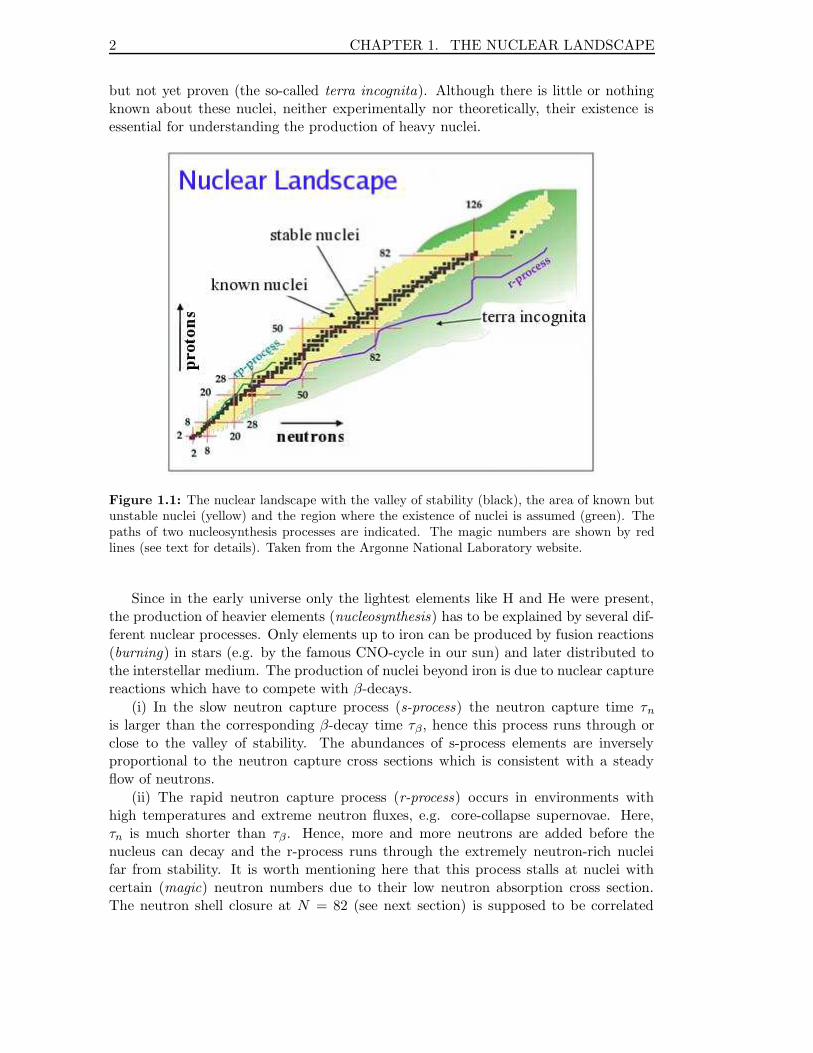
The nucleus is then determined by its charge number Z (i.e. its number of protons)and its number of neutrons N (or its mass number A = Z + N). It is usually notedAZXN with X being the chemical symbol. Today, there are nearly 3000 nuclei known,out of which less than 300 are stable. In a nuclear chart, all these nuclei are drawncorresponding to their Z and N values. In figure 1.1 such a nuclear chart is shownwith the valley of stability indicated in black and the area of known nuclei indicated inyellow. Also shown in this figure is the area where the existence of nuclei is assumed,
11 fm (femtometer) = 10−15 m. It is often called 1 fermi in honour of Enrico Fermi.
1
2 CHAPTER 1. THE NUCLEAR LANDSCAPE
but not yet proven (the so-called terra incognita). Although there is little or nothingknown about these nuclei, neither experimentally nor theoretically, their existence isessential for understanding the production of heavy nuclei.
Figure 1.1: The nuclear landscape with the valley of stability (black), the area of known butunstable nuclei (yellow) and the region where the existence of nuclei is assumed (green). Thepaths of two nucleosynthesis processes are indicated. The magic numbers are shown by redlines (see text for details). Taken from the Argonne National Laboratory website.
Since in the early universe only the lightest elements like H and He were present,the production of heavier elements (nucleosynthesis) has to be explained by several dif-ferent nuclear processes. Only elements up to iron can be produced by fusion reactions(burning) in stars (e.g. by the famous CNO-cycle in our sun) and later distributed tothe interstellar medium. The production of nuclei beyond iron is due to nuclear capturereactions which have to compete with β-decays.
(i) In the slow neutron capture process (s-process) the neutron capture time τn
is larger than the corresponding β-decay time τβ, hence this process runs through orclose to the valley of stability. The abundances of s-process elements are inverselyproportional to the neutron capture cross sections which is consistent with a steadyflow of neutrons.
(ii) The rapid neutron capture process (r-process) occurs in environments withhigh temperatures and extreme neutron fluxes, e.g. core-collapse supernovae. Here,τn is much shorter than τβ. Hence, more and more neutrons are added before thenucleus can decay and the r-process runs through the extremely neutron-rich nucleifar from stability. It is worth mentioning here that this process stalls at nuclei withcertain (magic) neutron numbers due to their low neutron absorption cross section.The neutron shell closure at N = 82 (see next section) is supposed to be correlated
1.1. THE NUCLEAR CHART 3
with the A ≈ 130 peak in the solar-system abundance of heavy elements.
(iii) The rapid proton capture process (rp-process) can occur especially in hydrogen-rich environments at high temperatures (Wallace and Woosley, 1981). It is consideredto play a substantial role in the production of nuclei on the neutron-deficient side ofstability, e.g. it explains very well the observed abundances of neutron-deficient nucleiwith A . 100 (Schatz et al., 1998).
Among the most important nuclear properties for understanding and modeling theseprocesses are nuclear half-lives, separation energies (or masses) and neutron capturecross sections. Since experimental data far off stability is scarce, these properties oftenhave to be deduced from nuclear models. The aim of nuclear structure physics isthen to improve these models by gathering further experimental data on these nuclei,describing and interpreting nuclear properties and by probing the interaction betweennucleons.
There are two complementary approaches to describe the nucleus:
(i) a microscopic approach, where nucleons are treated as independent particlesmoving in a central potential arising from the interaction of each nucleon with all othernucleons. One of the simplest such models is the so-called Fermi gas model in whichthe nucleons are considered as non-interacting particles in a 3-dimensional square wellpotential. This leads to energy eigenvalues E ∝ (n/d)2 where n is the radial quantumnumber and d the size of the well. The total kinetic energy of this system is thenEtot ∝ (N − Z)2 which is consistent with the stable nuclei having N ≈ Z. For A & 40the repulsive Coulomb interaction between the protons leads to a neutron excess. Thismodel can be seen as predecessor of the successful shell model (see next section).
(ii) a macroscopic approach where the nucleus is treated like a macroscopic (orgeometric) object. One of the earliest nuclear models, the liquid drop model (firstdescribed by Gamow (1930)), belongs in this category. There, the nucleus is describedsimilar to a drop of an incompressible liquid. The observed masses and binding energiescan be well deduced from it (von Weizsacker, 1935). In this model the nucleus has asurface and a shape and excitations can be described in terms of collective vibration androtation. These ideas are also essential in the collective model by Bohr and Mottelson(1975).
For more details about both approaches see also Heyde (1999).
1.1.1 Properties of Nuclei and the Nuclear Force
From the fact that bound nuclei exist it can be seen that there must be an attractiveinteraction between the nucleons which is stronger than the repulsive Coulomb forcebetween the protons – the nuclear force. On the other hand it is known from scatteringexperiments that the nuclear density is nearly constant. This shows that there must bea repulsive core at very short distances. The volume of the nucleus then has to increaseas V ∝ A, hence the mean nuclear radius can be defined as R = R0 · A1/3 with R0
being a constant between 1.2 fm and 1.3 fm.
The mass of a nucleus can be expressed as the sum of the masses of the nucleons
4 CHAPTER 1. THE NUCLEAR LANDSCAPE
minus its binding energy2
M = Z ·mp +N ·mn −Eb.
It is interesting to note that for A & 20 the binding energy per nucleon Eb/A saturatesto about 8 MeV (cf. figure 1.2). This can be explained by assuming that nucleons
interact only with their nearest neighbours, i.e. the range of the nuclear force is onlyof the order of 1 fm.
Related to the binding energy are the neutron (proton) separation energies Sn (Sp).These are defined as the energies needed to remove a neutron (proton) from a nucleusAZXN to infinity. Hence, they are equal to the difference in binding energies betweenAZXN and A−1
Z XN−1 (A−1Z−1XN ). In general, the separation energies decrease with an
increasing number of like nucleons and increase with an increasing number of unlikenucleons (cf. figure 1.3). For certain values of Z or N the separation energies showlarge and sudden drops. These values turn out to be the so-called magic numbers (seesection 1.2). This behaviour is similar to the behaviour ionizationion energies in atomsand already hints to a certain analogy in structure. And just as a lot of knowledgeon atoms was gained by studying their excited states, a lot about nuclear structurecan be learned by studying nuclear excited states, their energies, spins and parities(the latter are usually denoted as Jπ). As an example, the energies of the first excitedstates are highest for nuclei with magic nucleon numbers and reach their minimum inthe mid-shell region which is another evidence for magicity in nuclei.
The behaviour of the separation energies shows that there is a strong attractivep-n-interaction, whereas the residual interaction between like nucleons is repulsive.
2Masses and energies are used equivalently and factors of c2 are skipped throughout this thesis.
1.2. NUCLEAR SHELL MODEL 5
Figure 1.3: Neutron separation energies near the N=82 magic number (from Casten (2000)).
However, looking closer at Sn (Sp), an oscillation between odd and even numbers ofneutrons (protons) can be seen. This hints to an attractive pairing interaction couplingneutrons (protons) to Jπ = 0+. Hence, the ground state in even-even nuclei is alwaysJπ = 0+.
More information on the nucleon-nucleon-interaction can be gained from data onmirror nuclei. These are nuclei where the proton and neutron number exchange, e.g.2713Al14 and 27
14Si13. The similarity of their level schemes (energies, spins and parities oftheir excited states) suggests that the nuclear force is charge independent, i.e. p-p-, p-n-and n-n-interactions are equal. However, this is only true for triplet state (T = 1). TheT = 0 component of the nuclear interaction can be very different. With the exampleof the deuteron it can be shown that the interaction of two unlike nucleons is moreattractive in the T = 0 state than in the T = 1 state (cf. Casten (2000)).
1.2 Nuclear Shell Model
The most important and successful model to describe nuclei microscopically is theshell model. As mentioned in the section above the shell model is a development ofthe independent particle model in which the nucleons are considered as non-interactingparticles moving in a central potential U(~r). The main difference to the description ofelectrons in atomic physics stems from the fact that the central potential is producedby the nucleons itself. Therefore, the basis for this potential has to be the two-body
6 CHAPTER 1. THE NUCLEAR LANDSCAPE
nucleon-nucleon interaction Vik. The resulting Hamiltonian is then:
H =A∑
i=1
− ~2
2mi∆i +
A∑
i>k=1
Vik(~ri − ~rk). (1.1)
Since this Hamiltonian becomes practical unsolvable for increasing A it needs to besimplified. This is done by introducing a mean field in which all nucleons move:
H =
[
A∑
i=1
− ~2
2mi∆i + Ui(~r)
]
+
[
A∑
i>k=1
Vik −A∑
i=1
Ui(~r)
]
= H0 +Hres. (1.2)
The central potential U(~r) is chosen such that Hres is a small perturbation compared toH0. This can be achieved in a self-consistent approach, starting from effective nucleon-nucleon interaction, by Hartree-Fock methods. With a reasonable nuclear potentialthe solutions of the Schrodinger equation for the unperturbed Hamiltonian H0 shouldreproduce the observed magic numbers:
[
A∑
i=1
− ~2
2mi∆i + Ui(~r)
]
Ψ(~r) =
[
A∑
i=1
h(i)0
]
Ψ(~r) = EΨ(~r). (1.3)
The single-particle equations are then given by h(i)0 ψi = εiψi with
Ψ(~r) =∏
i
ψi and E =∑
i
εi.
In spherical coordinates the equation is usually simplified by separating the wave func-tion in its radial and angular coordinates. The resulting wave function is then givenby
ψ(~r) = Rnl(r)Ylm(θ, φ)
with −l ≤ m ≤ l and energy eigenvalues Enl (see e.g. Heyde (1999) for details).The radial solutions of the Schrodinger equation Rnl(r) show that states with highern have higher energy and that – for the same n – states with higher l have higherenergies. These two effects can counterbalance and lead to the grouping of levels atsimilar energies with larger gaps in-between. A reasonable first approximation for thecentral potential is the harmonic oscillator potential
U(r) =1
2mω2r2 (1.4)
which results in energy eigenvalues
Enl =
(
2n+ l − 1
2
)
~ω =
(
N +3
2
)
~ω (1.5)
with N = 2(n − 1) + l being the principle quantum number. The energy levels aredegenerated multiplets defined by the values of 2n+ l.
Including the intrinsic spin of the nucleons s = 1/2 the total angular momentumquantum number can be defined as j = l ± 1/2. The number of nucleons per or-bit is then limited to 2j + 1. The magic numbers resulting from this potential are
1.2. NUCLEAR SHELL MODEL 7
2, 8, 20, 40, 70, 112 . . . which deviates from observation for A ≥ 40. Therefore, somemodifications to this potential are necessary. Since nucleons with angular momentumexperience a centrifugal force, an additional term Ucent appears in the potential
Ucent =
∫
mω2r2dr =
∫
L2
mr3dr =
l(l + 1)~2
2mr2
which is proportional to l2. This term effectively flattens the potential in the centerwhich is quite reasonable since nucleons in the center are uniformly surrounded by othernucleons and should feel no net force. This modification breaks some of the degeneracyof the simple harmonic oscillator potential levels, but still does not reproduce theobserved magic numbers.
It was the ground-breaking idea of Mayer (1950) and – independently – Haxel et al.(1950) that the potential should include a spin-orbit coupling term U ls(r) = α(r)l · s.Here, l is the orbital angular momentum operator and s the intrinsic spin operator.This term stems from a quantum relativistic effect and is more difficult to describeintuitively. However, as nucleons in the center feel no net force, the spin-orbit forcecan be regarded as a surface phenomenon with α(r) = −Uls · ∂
∂rU(r). It is worthemphasizing here that absolute strength of the spin-orbit coupling must be of the samemagnitude as the central potential itself to reproduce the correct magic numbers.
The coupling term can be rewritten using the total angular momentum operatorj = l + s. There are then two slightly different potentials and hence different energyeigenvalues for the different values of j:
εnlj =
2n+ l − 1
2
~ω + α
−l: j = l + 1/2
l + 1: j = l − 1/2(1.6)
With this approach the resulting magic numbers are 2, 8, 20, 28, 50, 82, 126 in accor-dance with the experimental data (see figure 1.4). However, it should be noted thatthe harmonic oscillator potential is infinite and has the wrong asymptotic behaviour.In practice, finite potentials like the more realistic Woods-Saxon potentials of the form
U(r) =U0
1 + exp[(r −R0)/a]+ Uls(r)
are often used.
1.2.1 Collectivity & Deformation
In practice the use of the shell model is rather limited. It works best for nuclei withonly one or a few nucleons3 outside a closed shell, i.e. valence nucleons. However, themore valence nucleons are present the more important residual interactions become andnuclear structure physics today concentrates a lot on the nature of these interactionsand their effects on the level scheme.
The residual interactions, described by the term Hres in eq. 1.2, can be expanded inits multipoles. The monopole term describes the single particle energies of the nucleonswhereas the higher-order terms will be responsible for the excitation spectrum of thenucleus. Among these excitations it is the electric quadrupole (E2)4 mode which is
3These could also be holes in this sense.4The nomenclature used here is EL or ML for electric or magnetic transitions of multipole order 2L.
8 CHAPTER 1. THE NUCLEAR LANDSCAPE
Figure 1.4: Level scheme of the shell model: on the left for the simple harmonic oscillatorpotential, in the middle modified by the l2 term and on the right including the spin-orbitcoupling term. Taken from Casten (2000).
of peculiar interest for this work. The low-energy E2 excitations can be interpretedas vibrational and rotational modes of the nucleus. This oscillation in shape can bedescribed by a new parametrization of the nuclear radius in the intrinsic frame
Rosc = R ·[
1 +∑
m
αmY2m(θ, φ)
]
(1.7)
with R being the mean nuclear radius as mentioned in section 1.1, Y2m being sphericalharmonics of order 2 and m being the magnetic substates. The expansion coefficientsαm can be expressed as
α0 = β cos γ and α2 = α−2 =1√2β sin γ.
The other two coefficients α±1 are zero in the intrinsic frame. Here, β represents thequadrupole deformation and γ describes the axial asymmetry. Most nuclei are (almost)axially symmetric, i.e. γ = 0.
1.3. EVOLUTION OF NUCLEAR STRUCTURE 9
For mid-shell nuclei with many valence nucleons alternatives to the shell model areinevitable. Two further developments are worth mentioning here, both involving theconcept of a nonspherical shape. In the deformed shell model (or Nilsson model) theindependent particle motion in a field of nonspherical shape is considered whereas inthe collective model the macroscopic motions and excitations of a nucleus having thisshape are described. As pointed out above the residual interactions are responsible forthe deformation from spherical shape and for the collective behaviour of the nucleus.Among the residual interactions the pairing interaction (see section 1.1) should oncemore be emphasized here: it couples like nucleons to J π = 0+ states, hence the ground-state in all even-even nuclei is a 0+ state and the first excited state in (almost) all even-even nuclei is a 2+ state. Therefore, the transition from the ground-state to the firstexcited state (and vice versa) is an electric quadrupole (E2) transition. Since collectiveeffects in low-lying states are of quadrupole character the study of these transitions isof great interest for nuclear structure physics (see also Casten (2000)).
1.3 Evolution of Nuclear Structure
When studying nuclear structure over a wide range in the nuclear chart, e.g. fromshell closures up to mid-shell regions, one studies the increasing influence of residualinteractions and collective properties become more important. The degree (and type)of collectivity can be expressed in terms of the energy ratio of the first 4+ state to thefirst 2+ state, i.e. R42 = E(4+
1 )/E(2+1 ). This ratio is one of the key signatures for
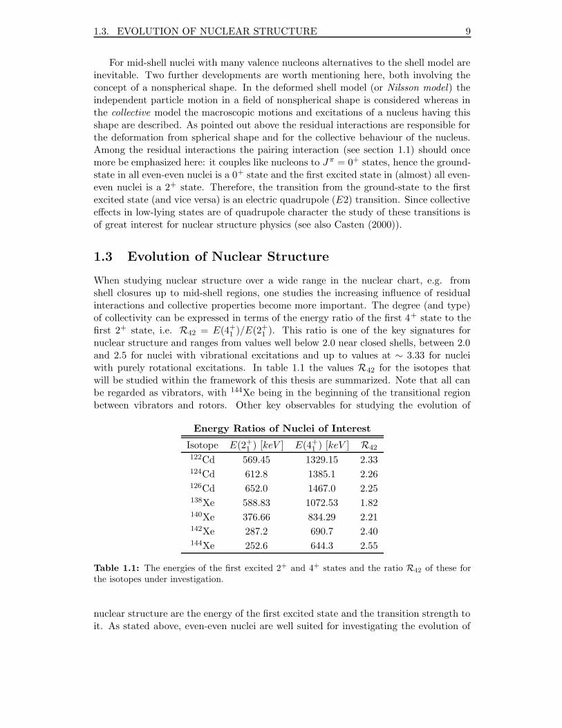
nuclear structure and ranges from values well below 2.0 near closed shells, between 2.0and 2.5 for nuclei with vibrational excitations and up to values at ∼ 3.33 for nucleiwith purely rotational excitations. In table 1.1 the values R42 for the isotopes thatwill be studied within the framework of this thesis are summarized. Note that all canbe regarded as vibrators, with 144Xe being in the beginning of the transitional regionbetween vibrators and rotors. Other key observables for studying the evolution of
Table 1.1: The energies of the first excited 2+ and 4+ states and the ratio R42 of these forthe isotopes under investigation.
nuclear structure are the energy of the first excited state and the transition strength toit. As stated above, even-even nuclei are well suited for investigating the evolution of
10 CHAPTER 1. THE NUCLEAR LANDSCAPE
collectivity. The first excited state is then the 2+1 state and the strength of the 0+
1 → 2+1
transition is expressed in terms of the reduced E2 matrix element (see chapter 2 fordetails):
B(E2 : Ji → Jf ) =1
2Ji + 1|〈Ψf ||E2||Ψi〉|2. (1.8)
In figure 1.5 the B(E2) values as well as the energies of the first excited 2+1 state for
isotopes around the neutron shell closure N = 82 are shown. As expected, the energyof the first excited state is increasing towards the closed shell and the probability toexcite a nucleus is increasing with the number of valence nucleons available to createthe excited state. Note that two contradicting B(E2) values for 140Xe exist in theliterature. The value of B(E2) = 0.324 e2b2 has been published in Cheifetz et al.(1980) whereas the higher value of B(E2) = 0.547 e2b2 has been determined from alifetime measurement by Lindroth et al. (1999). The general trend that an increasingE(2+
1 ) is accompanied by a decreasing transition strength, i.e. B(E2) ∝ 1/E(2+1 ),
can be derived from the liquid drop model for vibrational states (see Ring and Schuck(2000)). The systematic behaviour of these two observables has originally been studiedby Grodzins (1962) for a wide range of even-even nuclei. Further refinement has beendone by Raman et al. (2001) and Habs et al. (2002), resulting in a phenomenologicalrule that states that the product of B(E2) and E(2+
Here, Z denotes the charge number, N the neutron number and A = Z +N the massnumber of the nucleus under investigation. The term (N − N) is a measure for theneutron excess of the isotope with N being the neutron number for which the nuclearmass reaches its minimum within an isobaric chain. The parameters have been fittedto values known for nuclei with 48 ≤ Z ≤ 70 and R42 ≥ 1.8. In this thesis eq. 1.9 willreferred to as modified Grodzins rule.
1.4 Nuclei far from Stability
When going away from stability to nuclei with extreme N/Z ratios new phenomena canoccur, either due to changes of the spin-orbit coupling or due to residual interactionswhich become stronger. Among the latter, the so-called tensor force (i.e. a spin-isospindependent part of the nucleon-nucleon interaction) has been recognized to play a majorrole for the evolution of shell structure towards exotic nuclei.
Otsuka et al. (2001) showed that the tensor force can change the shell structure sig-nificantly for nuclei with large N/Z ratios. His calculations showed that the well-knownN = 20 shell gap at Z ≈ 14 decreases and even disappears when going to smaller chargenumbers and a new magic number N = 16 appears at Z = 8, predicting 24O to be adoubly-magic nucleus. This has just recently been confirmed experimentally (Kanungoet al., 2009)).
The tensor force has also been shown to modify nuclear shell structure throughoutthe nuclear chart (Otsuka et al., 2005) and to cause a reduction of the spin-orbit
1.4. NUCLEI FAR FROM STABILITY 11
N75 80 85 90
]2 b2) [
e+ 1
2→+
B(E2
;0
0
0.5
1
N75 80 85 90
]2 b2) [
e+ 1
2→+
B(E2
;0
0
0.5
1
CdTeXeBa
N75 80 85 90
) [ke
V]+ 1
E(2
0
500
1000
1500
N75 80 85 90
) [ke
V]+ 1
E(2
0
500
1000
1500 CdTeXeBa
Figure 1.5: Top: The B(E2) values for selected isotopes around N = 82 are shown along withthe values derived from the modified Grodzins rule (dashed lines; see text for details). Bottom:The energies of the first excited state in the same selection of isotopes. The lines emphasizethe systematic distribution around the shell closure.
12 CHAPTER 1. THE NUCLEAR LANDSCAPE
splitting with increasing neutron excess (Otsuka et al., 2006). The latter can also beexplained by a larger surface diffusiveness in neutron-rich exotic nuclei.
Schiffer et al. (2004) have shown that the spin-orbit splitting is decreasing withincreasing neutron excess by comparing the binding energies of the last proton outsidethe closed shell in Z = 51 nuclei and the binding energy of the last neutron in N = 83isotones. The question whether this is due to the tensor force or due to a surface effectremains open. Probing the stability of shell closures in exotic nuclei has thereforebecome one of the major issues in nuclear structure physics.
As mentioned before, the nucleosynthesis processes slow down at nuclei with closedneutron shells due to their low neutron absorption cross sections. These particularnuclei are called waiting-point nuclei. Since the r-process involves very neutron-richnuclei, its modeling is very sensitive to changes in the shell structure in that regionof the nuclear chart. β- and γ-spectroscopic decay studies of the N = 82 r-processwaiting-point nucleus 130Cd performed at ISOLDE (see chapter 3) showed evidence forthe theoretical predicted N = 82 shell quenching (cf. Dillmann et al. (2003)) whereasrecent observation of the γ-decay of excited states in 130Cd at GSI did not show signsfor this shell quenching (Jungclaus et al., 2007).
The region around N = 82 has also drawn attention since the measurement of theB(E2) values of 132,134,136Te by Radford et al. (2002). As can be seen in figure 1.5these values deviate significantly from the prediction of the modified Grodzins rule. Itis especially the very low B(E2) value of the N = 84 nucleus 136Te that is puzzlingas its corresponding 2+
1 energy drops as much as those of the other isotopes shown.It would be expected that a decreasing E(2+
1 ) goes along with an increasing B(E2)value. The anomalous behaviour in the Te isotopes has been explained with a reducedneutron pairing above the N = 82 shell closure by Terasaki et al. (2002).
In order to shed further light on the behaviour of B(E2) values around N = 82,hence probing the stability of the shell closure and the evolution of collectivity aroundit, a systematic study of B(E2) values both below and above the shell gap seemsnecessary. In this thesis, the measurement of B(E2) values for 122−126Cd as well as for138−144Xe by means of Coulomb excitation experiments is reported.
In chapter 2 the theoretical framework of Coulomb excitation along with its appli-cation to this work is explained. The experimental setup is described in chapter 3 andthe process of data analysis for all reactions can be found in chapter 4. The results aresummarized and discussed in chapter 5.
—For knowledge, too, itself is
power.
Francis Bacon (1561-1626)
2Coulomb Excitation
The possibility of exciting nuclei by the long-range electromagnetic interaction wascalculated and realized already in the 1930s (Weisskopf, 1938). A major impetus toCoulomb excitation experiments occurred, however, with the suggestion of the nuclearrotational and vibrational model by Bohr and Mottelson in 1952 (Bohr and Mottelson,1975). Experimental evidence even preceded this suggestion, but was unrecognizedas such until repeated with several different nuclei (McClelland and Goodman, 1953).Since then, Coulomb excitation developed into an important tool for investigating low-lying nuclear states. In the case of pure (or safe) Coulomb excitation, the only nuclearproperties which enter into the theory are the matrix elements of the electromagneticmultipole moments of the initial and final states involved in the transition. Hence,one of the great advantages of Coulomb excitation is that it depends solely on theelectromagnetic coupling, which is one of the best understood phenomena in presentday physics.
2.1 Semi-Classical Treatment
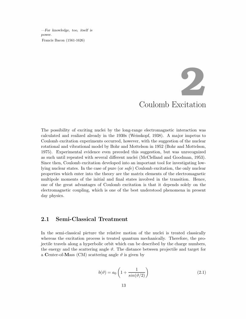
In the semi-classical picture the relative motion of the nuclei is treated classicallywhereas the excitation process is treated quantum mechanically. Therefore, the pro-jectile travels along a hyperbolic orbit which can be described by the charge numbers,the energy and the scattering angle ϑ. The distance between projectile and target fora Center-of-Mass (CM) scattering angle ϑ is given by
b(ϑ) = a0
(
1 +1
sin(ϑ/2)
)
(2.1)
13
14 CHAPTER 2. COULOMB EXCITATION
with a0 = Z1Z2e2
2ECMand ECM = 1
2µv2∞ = A2
A1+A2E1 the energy of the reaction in the CM
system1 (cf. figure 2.1). Here, the subscript 1 (2) denotes variables belonging to theprojectile (target). A sufficient requirement for ensuring that the projectile does not
ProjectileTarget
b(Θ)Θ
Figure 2.1: Coulomb Scattering in the Center-of-Mass System
penetrate the target nucleus (safe Coulomb excitation) is that its deBroglie wavelengthλ is smaller than half the distance of closest approach:
b(ϑ = 180)
2λ=Z1Z2e
2
~v∞=: η 1. (2.2)
The parameter η is called Sommerfeld parameter (Sommerfeld, 1931). The differentialcross section for exciting a nucleus from an initial state |i〉 to a final state |f〉 is givenby
(
dσ
dΩ
)
if
=
(
dσ
dΩ
)
Ruth
· Pif
where Pif is the transition probability and(
dσdΩ
)
Ruth=(
a0
2
)2sin−4(ϑ/2) is the well-
known Rutherford cross section. The excitation process can be described with the timedependent Schrodinger equation
i~∂
∂t|Ψ(t)〉 = H0 + V (~r(t))|Ψ(t)〉 (2.3)
where V (~r(t)) is the operator of the electromagnetic interaction andH0 the Hamiltonianof the free nucleus. Solving this equation with the initial condition that at t = −∞ thenucleus is in its ground state, i.e. |Ψ(−∞)〉 = |0〉, leads to the wave function of thenucleus after the collision:
Ψ(~r, t) =∑
f
αif (t)Ψf (~r) =∑
f
αif (t)|f〉. (2.4)
Here, the sum is over all possible final states and the coefficients αif are the excitationamplitudes. The probability for a transition |i〉 → |f〉 is then
Pif = |αif |2. (2.5)
1µ is the reduced mass of the target and projectile nuclei, v∞ denotes the relative velocity of theseat large distances.
2.1. SEMI-CLASSICAL TREATMENT 15
So far the energy loss∆E = Ef −Ei
has been neglected. For the validity of the semi-classical picture it has to be shown thatthis energy loss does not modify the orbit significantly, i.e. ∆E/ECM 1. A nucleuscan only be excited to the state |f〉 if the collision time τcol = a0/v, i.e. the time ittakes the projectile to travel the distance of closest approach, is shorter or equal to theexcitation time τexc = ~/∆E. This can be described by the adiabaticity parameter ξ:
ξ =τcol
τexc=a0∆E
~v≤ 1. (2.6)
If the collision time is longer the nucleus is able to follow the perturbation causedby V (~r(t)) adiabatically and the excitation probability decreases exponentially with ξ.The abovementioned energy loss can now be rewritten as
∆E/ECM = 2ξ/η.
If η 1 and ξ ≤ 1 the usage of the semi-classical picture is reasonable. In a similarmanner it can be shown that the angular momentum transfer does not alter the orbitsignificantly. The total orbital angular momentum can be written as l ≈ µva0 = ~ηand the difference before and after the collision is given by ∆l = L~ (here, L is themultipolarity of the transition). Hence, ∆l/l 1 is automatically fulfilled for safeCoulomb excitation. In table 2.1 the values of the relevant parameters for the differentexperiments performed in the framework of this thesis are given. Since the scattering
Table 2.1: Relevant parameters for the experiments described in this work (see text for details).The minimum distance ∆ for the experimental range in ϑ is given.
process is treated semi-classically the condition for safe Coulomb excitation can beinterpreted geometrically such that the nuclei should always be kept at a certain safetydistance ∆ of at least ≈ 5 fm (Wilcke et al., 1980). This is fulfilled if always
b(ϑ) ≥ R1 +R2 + ∆
with Ri = 1.25A1/3i fm (i=1,2). In figure 2.2 it is shown that in the experiments
described in this work the safety distance is always larger than 7 fm.
16 CHAPTER 2. COULOMB EXCITATION
[deg]CMθ50 100 150
) [fm
]θ
b(
0
20
40
60
80
100
[deg]CMθ50 100 150
) [fm
]θ
b(
0
20
40
60
80
100Pd108Cd on 122
Pd104Cd on 124
Zn64Cd on 124
Zn64Cd on 126
Mo96Xe on 138
Mo96Xe on 140
Mo96Xe on 142
Mo96Xe on 144
∆
Figure 2.2: The distance b(ϑ) and R1 +R2 for the different experiments is shown. It can be seenthat the distance ∆ is always larger than 5 fm.
2.2 First Order Perturbation Theory
The strength of the interaction potential V (~r(t)) between projectile and target can beexpressed in terms of the matrix elements of the action integral (measured in units of~ (Alder and Winther, 1975)):
χif (ϑ) = 〈f |∫ +∞
−∞
V (~r(t))dt|i〉
≈ 〈f |V (b(ϑ))|i〉τcol
(2.7)
which has been estimated by the value of V at closest approach and the collision time.It is convenient to define this parameter for ϑ = π as
χif = ±√
Pif (ϑ = π, ξ = 0).
If this parameter is small compared to unity, i.e. if the interaction V is weak, theexcitation amplitudes can be calculated using a first-order perturbation approximation.They are then given by
αif =1
i~
∫ +∞
−∞
〈f |V (~r(t))|i〉exp(iωt)dt (2.8)
with ∆E = ~ω. The electromagnetic interaction between target and projectile can bedecomposed in its multipole components. The monopole-monopole part leads to elas-tic (or Rutherford) scattering whereas the monopole-multipole and multipole-multipole
2.3. HIGHER-ORDER PERTURBATION THEORY 17
components induce inelastic scattering and hence the excitation of the nuclei. Corre-spondingly the parameter χ can be decomposed into partial sums
χ =∑
L
χ(L),
where each term belongs to the part of V (~r) which has multipole order L. The ex-citation amplitudes are then factorized into a part that depends only on the matrixelements of the multipole components and a part that depends only on the parametersof the classical orbit. It can be shown (Alder and Winther, 1975) that
αif ∝∑
L,M
1
2L+ 1〈i|M(EL,M)|f〉∗REL(ϑ, ξ) (2.9)
for electric excitation. Here, the dimensionless orbital integrals REL(ϑ, ξ) have beenintroduced. These depend on the adiabaticity parameter ξ and will vanish in theadiabatic limit ξ 1 as REL ∝ exp(−ξ). They measure the excitation probabilityrelative to the case of ϑ = π and ξ = 0. The matrix elements are defined generally as
M(EL,M) =
∫
ρ(~r)rLYL,M(r)d3r (2.10)
with ρ(~r) the charge density and YL,M the spherical harmonics. With the definition ofthe reduced transition probability (see eq. 1.8)
B(EL; Ji → Jf ) =∑
M,Mf
|〈JfMf |M(EL,M)|JiMi〉|2
=1
2J0 + 1|〈Jf ||M(EL)||Ji〉|2
(2.11)
the differential cross section turns out to be
dσEL =
(
Z1e
~v
)2
a−2L+20 B(EL)dfEL(ϑ, ξ). (2.12)
The function dfEL holds the relation dfEL ∝ R2EL(ϑ, ξ)sin−4(ϑ/2)dΩ. The total electric
excitation cross section is then given by
σEL =
(
Z1e
~v
)2
a−2L+20 B(EL; Ji → Jf )fEL(ξ). (2.13)
2.3 Higher-order Perturbation Theory
If the parameter χ is larger than or comparable to unity the Coulomb excitation processmust be treated by directly solving the time dependent Schrodinger equation (eq. 2.3).However, in practice the deviation from first-order can often be described by secondorder corrections. The perturbation expansion is a series expansion in χ and is expected
18 CHAPTER 2. COULOMB EXCITATION
to converge for χ at most of the order of 0.5. The excitation amplitudes αif are thengiven by (Alder and Winther, 1975)
αif = α(1)if +
∑
z
α(2)izf (2.14)
where the first term is the known first-order excitation amplitude and
α(2)izf =
(
1
i~
)2 ∫ +∞
−∞
〈f |V (~r(t))|z〉exp(iωt)dt ×∫ t
−∞
〈z|V (~r(t′))|i〉exp(iω′t′)dt′ (2.15)
with ~ω = Ef − Ez and ~ω′ = Ez − Ei. Here, a summation over a complete set ofintermediate nucular states |z〉 is performed. Two cases of second order effects areworth mentioning here:
Two Step Excitation
The final state |f〉 may be excited directly or through a low-lying state |z〉 (cf. fig-ure 2.3). In practice, a two-step excitation is realized if the direct excitation |i〉 → |f〉is small or forbidden, i.e. χif << χiz · χzf . An interesting case is that of a two-stepexcitation from the 0+ ground state to a 4+ state through an intermediate 2+ state.Since the direct excitation can only take place via an E4 transition - which is usu-ally quite weak - the two-step excitation process strongly dominates. The excitation
probability is then P(2)if ∝ |χ(2)
iz |2 · |χ(2)zf |2.
|Ji >
|Jz >
|Jf >
χzf
χiz
χif
|Ji >
|Jf >
χif
χff
Figure 2.3: Left: Schematic view of a two-step excitation through an intermediate state |z〉.Right: If the intermediate state is identical to the final state transitions between the magneticsubstates of |f〉 are taken into account by the diagonal matrix element (see text for details).
Reorientation Effect
In cases where the intermediate state is identical to the initial or final state an in-teraction with the quadrupole moment of that state occurs (cf. figure 2.3 (right)).Considering the excitation of a 2+ state in an even-even nucleus the strength of this
2.4. APPLICATION TO EXPERIMENT 19
interaction depends on χ(2)2→2. This property is proportional to the intrinsic quadrupole
moment Q0 of the 2+ state:
χ(2)2→2 =
4
15
√
π
5
Z1e
~v
1
a20
〈2||M(E2)||2〉 with (2.16)
〈2||M(E2)||2〉 =
√
7
2π
5
4eQ0. (2.17)
Note that the quadrupole moment is related to the deformation parameter β (seesection 1.2) via
eQ0 =3√5πZR2
0e(
β + 0.16β2)
. (2.18)
A positive deformation parameter β > 0 corresponds to prolate deformation whereas anegative value β < 0 corresponds to oblate deformation.
The change in the angular distribution of the γ-rays resulting from the second-ordertreatment is caused by transitions between different magnetic substates of the excitedstate. The excitation probability in second order is then given by (Schwalm et al., 1972;Alder and Winther, 1975)
P(2)02 = P
(1)02 (1 + qK(ξ, ϑ)) (2.19)
with
q =µ∆E
Z2〈2||M(E2)||2〉 (2.20)
and P(1)02 the excitation probability in first order. For projectile excitation, Z2 has to be
replaced by Z1. The excitation energy ∆E is given in MeV, while the reduced matrixelement 〈2||M(E2)||2〉 is given in e · b. The quantity K(ξ, ϑ1) depends only slightlyon the adiabaticity parameter ξ, but increases significantly with increasing scatteringangle. Typical values for K are of the order of unity.
2.4 Application to Experiment
The aim of the experiments described in this work is to determine the B(E2) values forthe 0+
1 → 2+1 and – in some cases – also the 2+
1 → 4+1 transitions of the projectile nuclei.
This has been achieved by measuring the gamma yields Nγ following the correspondingdisexcitation of both the projectile and the target nucleus. This gamma yield is
N (1),(2)γ ∝ σ(1),(2)
ce · ε(1),(2)γ · IBeam
with εγ being the total photopeak efficiency of the gamma detector array and IBeam
the beam intensity. A relative measurement of the Coulomb excitation cross sectionof the projectile nucleus to the known cross section for target excitation reduces thesystematic error stemming from uncertainties in these factors. The projectile excitation
20 CHAPTER 2. COULOMB EXCITATION
cross section is then given by:
σ(1)ce =
N(1)γ
N(2)γ
× ε(2)γ
ε(1)γ
× σ(2)ce and (2.21)
∆σ(1)ce
σ(1)ce
=
√
√
√
√
(
∆N(1)γ
N(1)γ
)2
+
(
∆N(2)γ
N(2)γ
)2
+
(
∆σ(2)ce
σ(2)ce
)2
. (2.22)
The variables N(1),(2)γ and ε
(1),(2)γ can be extracted from the experiment (see also sec-
tion 3.5 and chapter 4). Note that the uncertainties in the photopeak efficiency are of
the order of∆εγ
εγ∼ 10−3 whereas the uncertainties in σce and Nγ are 1-2 orders of mag-
nitude larger. Therefore, the contribution of (∆ε/ε)2 has been neglected here. Since
the target matrix elements - and therefore its Coulomb excitation cross section σ(2)ce
- are known, it is now possible to determine the projectile Coulomb excitation cross
section σ(1)ce . This cross section has to be reproduced by a theoretical calculation per-
formed with the code CLX (see section 2.6) depending on the matrix elements as inputparameters. Therefore, the B(E2) values of interest can be determined via linear inter-
polation between calculated cross sections σ(1)CLX for different matrix elements. These
calculations have to be corrected for the non-isotropic angular distribution of γ-rays(see section 2.5). Of course, in eq. 2.21 it is assumed that only the isotope of interest isresponsible for target excitation. For possible beam contaminations the gamma yield
N(2)γ has to be corrected.
2.5 Angular Distribution
Since the magnetic substates of |f〉 are not populated equally in Coulomb excitation,the emission of γ-rays is non-isotropic. A detailed discussion on the γ-ray angulardistribution can be found in Alder et al. (1956) or Alder and Winther (1975). Here,the results concerning the experiments in this work are described. It can be shown thatthe angular distribution of the emitted γ-rays can always be written in the form
W (θγ , φγ) =∑
k,k′
A∗
kk′(ϑ)Ykk′(θγ , φγ) (2.23)
with A∗
kk′(ϑ) =∑
κ,κ′
ρCκκ′(ϑ)Kkk′,κκ′
and ϑ being the scattering angle of the emitting particle. Ykk′(θγ , φγ) are the sphericalharmonics, ρC
κκ′(ϑ) is a statistical tensor which is the equivalent to the density matrixρC
κκ′ ∝ 〈f |ρ|i〉. Kkk′,κκ′ describes the effects of unobserved γ-rays, conversion electronsand other attenuating factors. If the particle is detected in a ring counter the angulardistribution is independent of φγ . For the case of an E2 transition the above formulasimplifies to
WE2(θγ) = 1 + a2P2(cosθγ) + a4P4(cosθγ) (2.24)
with Pn(cosθγ) being the Legendre polynomials.
2.6. COULOMB EXCITATION CALCULATIONS WITH CLX 21
Deorientation
An important phenomenon concerning the angular distribution of disexcitation γ-rays isthe nuclear deorientation effect. The initial nuclear alignment produced via Coulombexcitation may not be retained during the lifetime of the nuclear state. Hence, anattenuation of the angular distribution can be caused by hyperfine interactions betweenthe nucleus and the surrounding electron configuration. This leads to a modificationof eq. 2.24 by introducing time-dependent attenuation factors:
Assuming that the mean time between fluctuations of the electron configuration issmall compared to the lifetime of the nuclear state τN and small compared to theprecession time of the nuclear magnetic moment Abragam and Pound (1953) introducedthe following parametrization for these attenuation factors:
Gk(t) = exp [−λkt] and (2.26)
Gk =
∫
∞
0e−t/τNGk(t)dt/τN =
1
1 + λkτN. (2.27)
The integrated attenuation factors can be expressed in terms of a single relaxation timescale
τ2 = λ−12 ∝ 1
g2µ2N 〈H2〉1/2
with H being the magnetic field at the nucleus (cf. Danchev et al. (2005)). They arethen given by
G2 =τ2
τ2 + τNand G4 =
0.3τ20.3τ2 + τN
. (2.28)
In this work eq. 2.25 has been taken into account by means of the parameter λ2 asinput parameter for the coupled-channel code CLX (see section 2.6).
2.6 Coulomb Excitation Calculations with CLX
The Coulomb excitation calculations for this thesis were performed using the coupled-channel code CLX, originally written by H. Ower, adapted by J. Gerl and furthermodified by Th. Kroll. This code was used to calculate the differential and integratedexcitation cross sections of the projectile and target nuclei. It follows the nomenclatureof Alder and Winther (1975).
Its input parameters include
• the charge and mass numbers Z,A of the projectile and target nuclei
• the number of states involved in the calculation
• the spin, parity and energy for each of these states
• the beam energy
• the range in ϑp over which to integrate the cross section
22 CHAPTER 2. COULOMB EXCITATION
• the transitions |i〉 → |f〉 under consideration together with their matrix elementsME(i→ f) and their multipolarities2
• the positions(s) of the gamma detector(s)
• the conversion coefficients taken from Hager and Seltzer (1968)
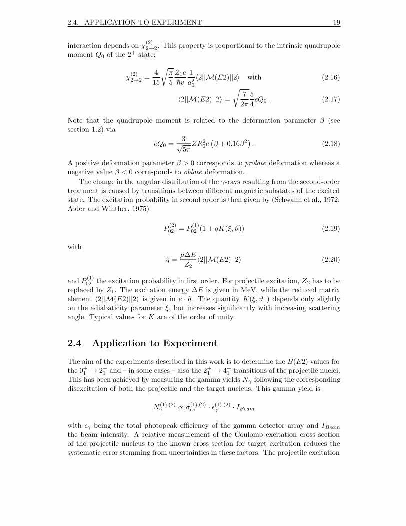
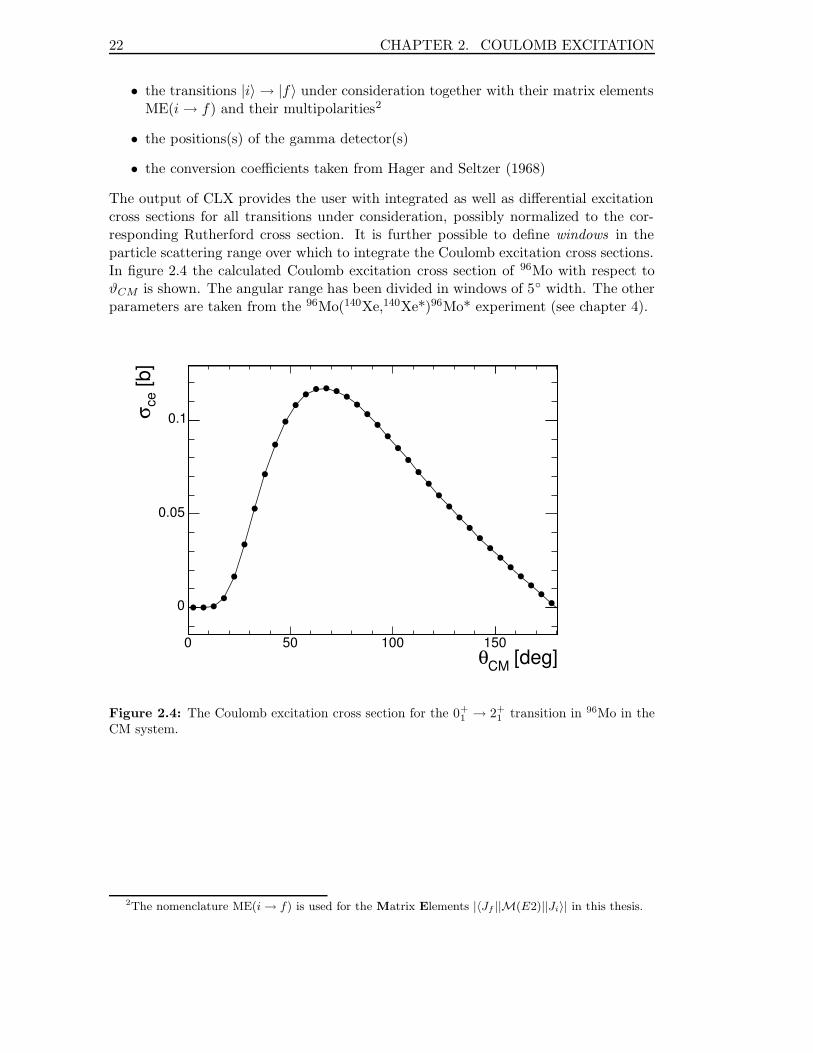
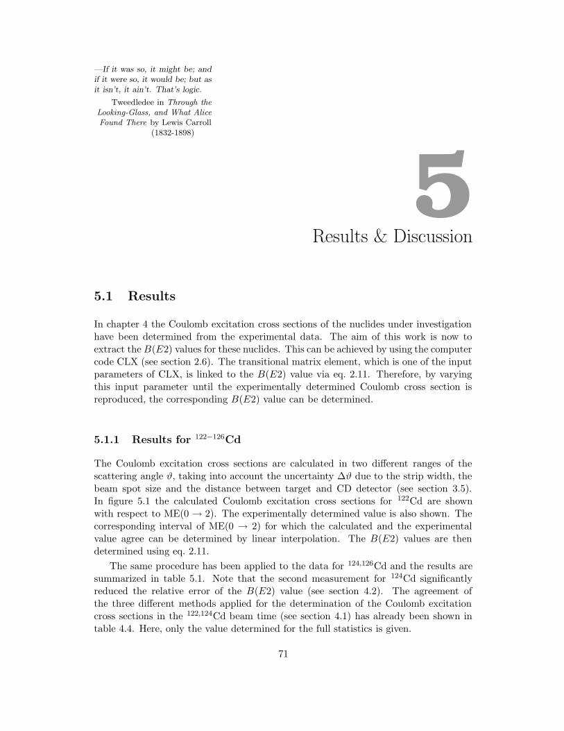
The output of CLX provides the user with integrated as well as differential excitationcross sections for all transitions under consideration, possibly normalized to the cor-responding Rutherford cross section. It is further possible to define windows in theparticle scattering range over which to integrate the Coulomb excitation cross sections.In figure 2.4 the calculated Coulomb excitation cross section of 96Mo with respect toϑCM is shown. The angular range has been divided in windows of 5 width. The otherparameters are taken from the 96Mo(140Xe,140Xe*)96Mo* experiment (see chapter 4).
[deg]CMθ0 50 100 150
[b]
ceσ
0
0.05
0.1
Figure 2.4: The Coulomb excitation cross section for the 0+1 → 2+
1 transition in 96Mo in theCM system.
2The nomenclature ME(i → f) is used for the Matrix Elements |〈Jf ||M(E2)||Ji〉| in this thesis.
—There is nothing new to be
discovered in physics now. All
that remains is more and more
precise measurement.
William Thomson, Lord Kelvin(1824-1907)
3Experimental Setup
For the investigation of nuclei far away from stability (exotic nuclei) the developmentof Radioactive Ion Beams (RIBs) is necessary. The isotopes of interest are createdby nuclear reactions such as fission, fragmentation, spallation and fusion. The latterproduces proton-rich nuclei whereas the others can lead to the neutron-rich side of thenuclear chart.
3.1 Methods of Producing RIBs
The development of RIB facilities with reaccelerated beams opened a new field ofnuclear physics since the 1990’s. Two different techniques of producing RIBs are usedin current RIB facilities: (i) the In-Flight projectile fragmentation (IF) method and(ii) the Isotope Separation-On-Line (ISOL) method which is used for the experimentsdescribed in this work. These techniques are very complementary regarding, e.g., theirenergy range.
3.1.1 In-Flight Method
The IF method consists of a high-energy beam of heavy nuclei impinging on a thin(∼ g/cm2) target. Part of the beam particles collide with the target nuclei whichleads to projectile fragmentation or fission and other nuclear reactions. The reactionproducts basically keep the forward momentum of the primary beam. The isotope ofinterest can be selected by applying electromagnetic and kinematical separators.
The advantage of this method is that the produced nuclei are available almostinstantly and without chemical selectivity. Hence, isotopes with lifetimes down to afew µs can be investigated. The beam energy - ranging from about 10 A·MeV up tothe order of 1 A·GeV - is well suited for nuclear reaction studies, but makes studies oflow-lying nuclear structure or astrophysics experiments very difficult. The beam is alsoof only modest quality concerning its beam spot size, energy precision and spread and
23
24 CHAPTER 3. EXPERIMENTAL SETUP
angular divergence. Facilities which make use of the IF method are e.g. NSCL (USA),GANIL (France), GSI (Germany) or RIKEN (Japan).
3.1.2 Isotope Separation On-Line
The ISOL method uses a light beam (e.g. protons) that impinges on a thick productiontarget. In principle, the same kind of nuclear reactions can take place as above, but thistime the reaction products are thermalized in the target. They diffuse out of the targetand are ionized, accelerated again and mass separated. Due to the second accelerationa much higher beam quality can be achieved and the beam energy can be varied froma few A·keV up to some A·MeV and higher.
This technique is especially suitable for nuclear structure and astrophysics experi-ments. The main drawback is the slow release time from the primary target, hence onecannot use this method for isotopes with life times τ ≤ 10 ms. The diffusion out of thetarget depends also on the chemical properties of the element (e.g. refractory elementsdo not come out of the source). The ISOL method is used e.g. at ISOLDE (CERN),HRIBF (USA), ISAC (Canada) or SPIRAL (France).
3.2 The ISOLDE Facility
ISOLDE is an on-line isotope separation facility located at CERN1 with about 40 yearsof experience in the production of low-energy radioactive ion beams. Today, more than600 isotopes of more than 60 elements are available.
A beam of 1.4 GeV protons provided by the PSB2 impinges on a primary target(e.g. UCx), where fission and spallation takes place. The reaction products diffuse outof the target and are subsequently ionized to a 1+ state, possibly also as molecules.Different ion sources are used, depending on the element of interest.
After extraction the beam is mass separated and distributed to the different exper-iments in the hall (see figure 3.1).
3.2.1 The PS Booster
The PS Booster (PSB) is a stack of four small synchrotrons where protons are pre-accelerated before injection into the CERN Proton Synchrotron (PS) (see figure 3.2).The PSB delivers short pulses (∼ 2.4µs) of high intensity (up to 3.2 × 10¹³ p/pulse).About six pulses in a PS supercycle of typically 12 pulses are available for ISOLDEwhich is equivalent to a DC proton current of about 2µA. These protons are thentransfered to one of the two target zones of ISOLDE.
3.2.2 Targets and Ion Sources
For the experiments described in this work a UCx primary target has been used. Duringthe Cd runs, a tungsten rod has been applied close to the target. The protons, nowimpinging on this so-called proton-to-neutron converter, create fast reaction neutrons
1Conseil Europeen pour la Recherche Nucleaire2Proton Synchrotron Booster
3.2. THE ISOLDE FACILITY 25
ROBOT
RADIOACTIVE
LABORATORY
GPS
HRS
REX-ISOLDE
CONTROL
ROOM
1-1.4 GeV PROTONS
EXPERIMENTAL HALL
NEW EXTENSION
Figure 3.1: View of the ISOLDE experiment hall after 2006 (taken fromhttp://isolde.web.cern.ch/isolde/).
which induce fission in the UCx target. This method helps to suppress proton-richisobaric spallation products and therefore improves the beam purity.
The diffusion time depends strongly on the chemical properties of the ions of interestand on the target temperature which can be increased up to about 2000C. For thesubsequent ionization several different ion sources are available at ISOLDE:
Surface Ion Source: The surface ion source is the simplest setup for ionizing atomsproduced in the target. It consists only of a tube (transfer line) made of a metalwhich has a higher work function than the atoms ionization potential (e.g. tan-talum or tungsten). A more recent development is a transfer line made of quartz,which improved the beam purity during the 124,126Cd experiments described insection 4.2. The transfer line can be heated up to ∼ 2400C to avoid long stickingtimes of the atoms on the surface and to ensure that ions are repelled from thesurface.
Hot Plasma Ion Source: The plasma ion source is used to ionize atoms that cannotbe surface ionized. The plasma is produced by a gas mixture (e.g. Ar and Xe)that is ionized by impact of accelerated electrons.
Cold Plasma Ion Source: For the production of noble gas isotopes the above setupis modified such that the transfer line between target and plasma is cooled by acontinuous water flow and therefore the isobaric contamination in the ISOLDEion beams is reduced. This has been used for the Xe beam experiments describedin this thesis.
26 CHAPTER 3. EXPERIMENTAL SETUP
Figure 3.2: Schematic representation of the CERN accelerator complex (taken fromhttp://isolde.web.cern.ch/isolde/)
Laser Ion Source: A more sophisticated technique now in use is the Resonant IonizationLaser Ion Source (RILIS). A laser beam is tuned precisely to the energy of astrong atomic transition in the isotope of interest and a second laser beam isused to excite an electron from that state to the continuum. Since the secondbeam does not have enough energy to excite an electron from the ground state,the RILIS can select not only a specific isotope but even isomeric states. Some-times, as in the Cd runs described in this work, a 3-step ionization scheme is usedwhere the first two beams excite the isotope of interest from the ground state tosubsequently higher lying states and the third beam excites the electron to thecontinuum (see figure 3.3).
It is possible to operate the RILIS in two different modes: (i) the “laser off”mode, where only surface-ionized contaminants are seen in the beam and (ii) the“laser on” mode, where additionally the laser-ionized isotope of interest is seen.By comparing the data between these two modes the amount and kind of beamcontamination can be estimated.
3.2.3 The Mass Separators
After ionization the particles are extracted with typically 60 kV producing a 60 keVbeam. For selecting the ions of interest, two different mass separators are available at
3.3. REX-ISOLDE 27
continuum
510.6 nm
643.8 nm
228.8 nm
5s2 1S0
5s5p 1P1
5s5d 1D2
Figure 3.3: Ionization scheme for Cd and schematic view of the RILIS (taken fromhttp://isolde.web.cern.ch/isolde/).
ISOLDE, each with its own target. The so-called General Purpose Separator (GPS) isdesigned to allow three ion beams within a mass range of ±15% and a mass resolution ofM
∆M = 2400 to be selected and delivered to the experimental hall. The High-ResolutionSeparator (HRS) is designed for selecting one ion beam with a mass resolution ofM
∆M ≈ 5000.
3.3 REX-ISOLDE
The Radioactive Beam EXperiments (REX) facility was developed for bunching, chargebreeding and post accelerating the singly ionized RIBs coming from ISOLDE. In thefollowing, the REXTRAP, the EBIS and the REX linac are presented. A detailed de-scription can be found in Ames et al. (2005). A schematic view of its components isshown in figure 3.4.
3.3.1 REXTRAP
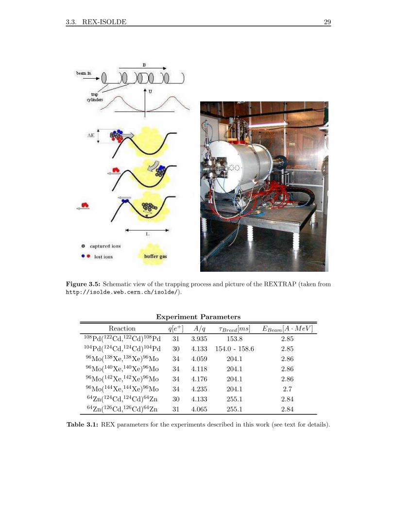
The REXTRAP is a Penning trap which was developed for accumulating, bunching andcooling of the singly-charged ions from the separators. Accumulation and bunchingis required for the ion injection into the subsequent charge breeder. Since the trappotential is 60 kV, the incoming ions have just enough energy to climb the first potentialthreshold. Once inside the trap, the ions are slowed down by collisions with a buffergas (typically Argon or Neon at a pressure of ∼ 10−3 mbar). After cooling, the ions areextracted to the EBIS in a bunch by lowering the ions potential threshold (see figure3.5).
28 CHAPTER 3. EXPERIMENTAL SETUP
Figure 3.4: Schematic view of the different parts of REX: the incoming beam is first accu-mulated in the trap, then charge bred in the EBIS and finally reaccelerated in the linac (takenfrom http://isolde.web.cern.ch/isolde/).
3.3.2 EBIS
The singly charged ions from the REXTRAP are injected into the Electron Beam IonSource (EBIS) in bunches. Inside the EBIS they are confined by the negative spacecharge of the electrons and by potential barriers established by cylindrical electrodes.For the injection into the linear accelerator (linac) a mass-to-charge ratio of A/q < 4.5is required. The trapped ions will therefore undergo stepwise ionization from 1+ ton+ via electron impact until a sufficient number of ions has reached this A/q value.For this, a mono-energetic electron beam from an electron gun focused by a strongmagnetic field (∼ 2T) is used. The energy of this beam is adjustable between 3 - 6 kV.
For the ionization process, an excellent vacuum (∼ 10−10 mbar) inside the EBIS isrequired. However, residual gas is still often seen as a contaminant in the subsequentexperiments. To obtain a high breeding efficiency, the phase space overlap of injectedions and the electron beam has to be large. Hence, a rather low extraction emittancefrom the Penning trap is needed. Unlike the trap, the potential of the EBIS platformis pulsed between injection and extraction from 60 to about 20 kV, allowing for a fixedion extraction velocity independent of the A/q-value.
The total breeding time can range from a few to a couple of hundreds of milliseconds.In table 3.1 these parameters are given for the experiments performed in the frameworkof this thesis.
3.3. REX-ISOLDE 29
Figure 3.5: Schematic view of the trapping process and picture of the REXTRAP (taken fromhttp://isolde.web.cern.ch/isolde/).
Table 3.1: REX parameters for the experiments described in this work (see text for details).
30 CHAPTER 3. EXPERIMENTAL SETUP
3.3.3 REX Linac
As the intensity of radioactive ions out of the EBIS is much smaller than the intensityof residual gas ions, a mass separator prior to the linac is required. This mass separatoris of the so-called Nier-spectrometer type (Nier and Roberts, 1951) and has reachedq/A-resolutions of ∼ 150. However, there will still be contaminants from residual gasisotopes with the same or similar A/q-values as the ion of interest in the beam. Thesecan typically be 14,15N,16,18O,20,22Ne,12,13C and 36,40Ar.
The linear accelerator consists of 4 different sections for stepwise accelerating theions extracted from the EBIS (cf. figure 3.6). The 5 A·keV ions from the EBIS are accel-erated to 300 A·keV by a Radio Frequency Quadrupole (RFQ). The RF quadrupolefield provides transverse focussing while a modulation of the four rods bunches andaccelerates the injected beam. The following IH (Interdigital-H-type)-structure accel-erates the ions from 0.3 A·MeV to an energy between 1.1 and 1.2 A·MeV. The outputof the IH structure is matched to the first out of three 7-gap resonators with a tripletlens. Between the first and the second resonator there is an additional doublet lens forfocussing. The three 7-gap resonators can accelerate the ions up to 2.3 A·MeV. Until2003 this has been the maximum beam energy at REX-ISOLDE.
These first three sections operate at 101.28 MHz, which is half the frequency ofthe CERN proton linac. In spring 2004 an energy upgrade up to 3 A·MeV has beenachieved by installing an additional 9-gap resonator which operates at 202.56 MHz.This upgrade has proven to be crucial for the ongoing Coulomb excitation experimentswith exotic nuclei, since it increases the Coulomb excitation cross section significantlywhich compensates for the low beam intensities when going away from stability. TheREX linac has a very compact design with a total length of only about 12m, sincespace was limited before the extension of the experimental hall in 2006.
Figure 3.6: Schematic view of the different parts of REX and the linac (taken fromhttp://isolde.web.cern.ch/isolde/).
3.4 The MINIBALL experiment
3.4.1 The Gamma Detector
The post-accelerated ion beam from REX is distributed to the experimental setup in-cluding the γ-ray detector array MINIBALL (see figure 3.7). MINIBALL consists of
3.4. THE MINIBALL EXPERIMENT 31
Figure 3.7: Bird view on the MINIBALL experimental site. On the right the end of the linacand the bending magnet can be seen. On the left the opened MINIBALL frame with the clusterscan be seen (taken from Niedermaier (2005)).
24 individually encapsulated HPGe3 detectors which are arranged in 8 triple clusters(cf. Eberth et al. (2001)). These clusters are mounted on six moveable arcs (the MINI-BALL frame) so that their position in θ and φ can be optimized with respect to solidangle coverage or experimental specific constraints (see figure 3.8). The clusters canalso be rotated around their axis by an angle α. In the setup used for this work thesolid angle coverage was ∼ 60% of the full 4π at a target-detector distance of about 10cm (cf. figure 3.9).
Since the beam coming from REX will have velocities up to β ∼ 0.1, the emitted γ-rays will be Doppler shifted. Therefore, a large granularity of the detector is requiredfor a reasonable Doppler correction. To achieve this, each detector is electronically6-fold segmented so that the overall granularity is 8 × 3 × 6 = 144 (cf. figure 3.10).The electronic segmentation is achieved by shielding parts of the crystal sides duringimplantation of Boron n-type impurities. In this way, only parts of the crystal areconnected and can be read out separately. The central electrode (the core), to whichthe depletion voltage is applied, will always detect an interacting γ-ray. It depends onthe interaction point in the crystal which segment will detect it. It is assumed thatthe first interaction is also the main interaction, i.e. the interaction in which mostof the energy is deposited. This plays a crucial role for the Doppler correction. Inthe so-called addback procedure the energies which are deposited in more than onecrystal within a cluster by one γ-ray are added and linked to the position of the first
3High Purity Germanium
32 CHAPTER 3. EXPERIMENTAL SETUP
Figure 3.8: The MINIBALL frame with its arms is shown (taken fromhttp://isolde.web.cern.ch/isolde/).
Figure 3.9: Close-up of the MINIBALL clusters surrounding the target chamber. The differentcolours indicate the three crystals per cluster and the different shades of each colour indicatethe segments (taken from http://isolde.web.cern.ch/isolde/).
3.4. THE MINIBALL EXPERIMENT 33
Segment
3
Segment
5
Segment
4
Segment
6
Segment
1
Segment
2
34 m
m
Figure 3.10: Schematic view of a cut through a MINIBALL crystal. The segments areindicated (by courtesy of Eppinger (2006)).
interaction. This increases the full energy peak efficiency, which is important whenworking with low-intensity RIBs. For more details on the MINIBALL spectrometer seealso Weißhaar (2003).
Typical depletion voltages are around 2.5 - 4.5 kV. The crystals are kept at liquidnitrogen (LN2) temperature by attaching dewars to each of the 8 clusters which areconnected with an autofill system.
3.4.2 The Particle Detector
For detecting the scattered beam particles as well as the target recoils, a Double SidedSilicon Strip Detector (DSSSD) has been mounted in the target chamber. This so-called CD detector consists of four quadrants, each of which is read out independently.The front side is segmented in 16 annular strips for measuring ϑ whereas the back sideconsists of 24 sector strips which were linked into pairs for measuring ϕ. The annularstrips have a width of 1.9 mm and a 2.0 mm pitch, the paired sector strips have a pitchof 6.8 (cf. figure 3.11). Each quadrant covers a range in ϕ of 81.6 and - at a targetdistance of 33 mm - the CD covers a range in ϑlab of 15 . ϑ . 51.
During the 138−142Xe experiments the inner four rings of the CD were covered bya plug in order to prevent the CD from damage due to high count rates of elasticallyscattered particles occurring at small scattering angles and to reduce the dead time ofthe particle detector. In the 124,126Cd and 144Xe experiments the CD has been shieldedby a degrader foil to reduce the energy of the detected particles.
34 CHAPTER 3. EXPERIMENTAL SETUP
Figure 3.11: Schematic view of the CD detector and its segmentation (see text) and pictureof one mounted quadrant (taken from Niedermaier (2005)).
3.4.3 Electronics and Data Acquisition
MINIBALL
The signals from the gamma detectors are integrated and amplified by the MINIBALLpreamplifiers and then fed into the XIA DGF4 modules (XIA, 2007) where they aredigitized with a sampling frequency of 40 MHz. Since each DGF has four input channelstwo modules are needed per crystal (one channel for the core signal and six morechannels for the segment signals, the remaining one stays empty). The digitized signalis further processed in an FPGA5 where digital filter operations are used to gain energyand time information. The FPGA generates an event trigger if a useable event ispresent. The pulse is then fed into the DSP6 and data read-out is forced. A detaileddescription can be found in Lauer (2004).
CD Detector
For each quadrant the signals from the 16 front and 12 back strips are fed into RAL 108preamplifiers and from there into RAL 109 shapers where both a Constant FractionTiming (CFT) and Gaussian-like shaping is performed. The logical OR of the timingsignals as well as the energy signals from each strip are fed into a CAEN V785 ADC7
module which generates the CD quadrant signal. The ORed timing signals are also fedinto a time stamp DGF which runs with the same 40 MHz clock as the DGF modulesused for MINIBALL. This is necessary for linking particle and gamma data, e.g. defin-ing a time difference between the detection of particles and γ-rays (see also figure 4.10).
4X-ray Instruments Associates, Digital Gamma Finder5Field Programmable Gate Array6Digital Signal Processor7Analog to Digital Converter
3.5. APPLICATION TO EXPERIMENT 35
Now for each particle event as well as for each gamma event an energy and a timestamp is stored. During the event building process the particles and the γ-rays withidentical time stamps can be put together into one event.
Another important timing signal is the EBIS signal which marks the injection ofions from the EBIS into the linac. This signal starts a time gate (the so-called On-beam window) during which data is taken. The end of the On-beam window triggersthe data read-out after which a second time gate with the same length (the so-calledOff-beam window) is opened during which again data is taken. This data can be usedto determine background radiation. Note that this data has to be read out before thenext EBIS pulse.
Other timing signals that are available are the PS signal, indicating the start of aPS supercycle, the T1 signal indicating that the proton beam impinges on the ISOLDEtarget and the T2 signal indicating that the ions are allowed into the trap.
More important, for experiments which make use of the RILIS (as those performedwith Cd beams for this thesis) a Laser flag signal indicating whether the laser was ’On’or ’Off’ is also stored.
The data acquisition is performed with Marabou which writes the raw data to .med
files (Lutter et al., 2009). This file format is based on the GSI MBS event structure. Acode developed at the MPI in Heidelberg (cf. Niedermaier (2005)) is used to transformthese into .root files containing a ROOT tree rt (see also Brun et al. (2009)).
3.5 Application to Experiment
The standard setup for all experiments described in this work consists of the MINIBALLgamma detectors, the particle detector, a PPAC8 for beam monitoring and a beamdump gamma detector at the end of the beam line (cf. figure 3.12). The isotope underinvestigation is delivered as radioactive ion beam by REX whereas a suitable target ischosen individually for each experiment (cf. table 3.2).
Several aspects are taken into account for this choice: (i) the target nucleus shouldhave a large enough and well-known Coulomb excitation cross section, (ii) the γ-energiesof the transitions involved should differ significantly from those in the projectile nucleus,so that the resulting peaks in the γ-spectra are separable and (iii) the mass A of thetarget nucleus should be chosen such that the target recoils can be separated fromthe projectiles kinematically. Of course, it can be rather difficult to fulfill all of theseaspects with an available target material.
For the determination of the B(E2) values the γ-ray yields from the ejectile andtarget disexcitation peaks are needed. Since these γ-rays are emitted in-flight theyhave to be Doppler corrected. For the Doppler correction the energies and scatteringangles of both the emitting particle and the γ-ray are needed and the following formulahas to be applied:
E′
γ = Γ ×Eγ × 1 − β [cos (θ) cos (ϑ) + sin (θ) sin (ϑ) cos (δφ)] . (3.1)
with δφ = ϕ−φ, Γ = 1/√
1 − β2 and β =√
2E/M (E being the particle energy). Theangles θ and φ belong to the γ-rays whereas ϑ and ϕ belong to the emitting particles.
8Parallel Plate Avalanche Counter
36 CHAPTER 3. EXPERIMENTAL SETUP
Figure 3.12: Schematic view of the experimental setup. The detection of projectiles and targetrecoils in the CD detector is indicated.
Table 3.2: The targets chosen for the experiments described in this work along with theirthicknesses and transitional matrix elements.
3.5.1 Position Calibration of the Gamma Detector
The angles (θ, φ, α) of the MINIBALL clusters - and therefore the positions of thecrystals - are determined using the 1-neutron pick-up reaction d(22Ne,23Ne)p. In this
reaction the first excited state in 23Ne(
Jπ = 12
+)
at 1017 keV is populated. It disex-
cites in-flight while the ejectile essentially moves in beam direction. Thus, the observedDoppler shift of the γ-ray can be used for the position calibration of the Ge detectors.The angular coordinates are varied recursively until (i) the FWHM9 of the Dopplercorrected peak in one cluster is minimized and (ii) the Doppler corrected peaks in the6 segments are aligned (see also van de Walle (2006)).
3.5.2 Position Calibration of the Particle Detector
In the Coulomb excitation experiments the angles of the particles can be determinedfrom the position sensitive CD detector. Of course, an uncertainty in this determinationremains. The uncertainty ∆ϑ in the scattering angle is of great importance for thefurther analysis, since it is not only needed in the Doppler correction, but also for the
9Full Width Half Maximum
3.5. APPLICATION TO EXPERIMENT 37
angular range over which the CLX calculations have to be integrated and for estimatingthe CD efficiency.
The position of the detected particle on the CD can be described by polar coordi-nates (r,ϕ) where the radius r is determined from the annular strip (ring) on the frontside and the angle ϕ from the radial strip on the back side. It is then
ϑ = arctan(r
d
)
(3.2)
∆ϑ =
√
(
∆rr
)2+(
∆dd
)2
1 +(
rd
)2 × r
d(3.3)
with ∆r =√
∆r2ring + ∆r2
spot and d being the distance between the target and the
CD detector. The beam spot size is estimated to be ∆rspot = 1 mm, the uncertaintydue to the ring width is ∆rring = 1 mm and the uncertainty in the distance is ∆d =1 mm. The calculated uncertainty ∆ϑ for each ring and an applied polynomial fitare shown in figure 3.13. The angular range of the CD detector in this setup is thenϑlab = 15(2) − 51(1).
[deg]θ20 30 40 50
[deg
]θ ∆
1.5
2
Figure 3.13: The uncertainty of the scattering angle is calculated for each ring. A polynomial fitof order 2 has been applied.
3.5.3 Energy Calibration of Particle Detector
The other variable determined from the CD and needed for the Doppler correction isthe particle energy. The CD detector was therefore calibrated using a triple α-source,
38 CHAPTER 3. EXPERIMENTAL SETUP
[deg]korrθ30 35 40 45 50
[MeV
]pa
rtE
50
100
150
200
500
1000
[deg]korrθ30 35 40 45 50
[MeV
]pa
rtE
50
100
150
200
250
0
10000
20000
30000
Figure 3.14: Particle energies for 140Xe and 96Mo as detected in the CD (left) and basedon kinematic calculations (right) vs. the corrected scattering angle in degrees. The correctionhas been applied due to a shift of the beam spot with respect to the center of the CD (seechapter 4).
consisting of 239Pu, 241Am and 244Cm with α-energies of 5.156 MeV, 5.486 MeV and5.805 MeV, respectively. Of course, the extrapolation of these energies to energiesof the order of ∼ 102MeV (as occur in the experiments described in this work) isproblematic. This is one of the reasons why in the later analysis the scattering angleϑ has been used to assign the particle energy via a look-up table based on kinematiccalculations including the energy loss in the target. Another reason is that the range ofthe preamplifiers of the CD detector is limited to about 200 MeV and that the degraderfoil used in later campaigns further distorts the energy signal. For the detection ofintermediate-mass and heavy ions, one has also to take care of the so-called pulseheight defect (see Knoll (1979)). This states that the charge produced by a heavyion in silicon is significantly less than the charge produced by a light ion depositingthe same energy and that this effect increases with the atomic number of the ion. Acomparison between the detected and the tabulated energy can be seen in figure 3.14.
3.5.4 Energy Calibration and Relative Efficiency of the Gamma De-tectors
For the energy calibration of the MINIBALL array source measurements with 60Coand 152Eu were used. The sources were placed at target position. First, the twoprominent lines of 60Co at 1173 keV and 1332 keV were used for a rough calibrationof the MINIBALL channels. Subsequently, the most prominent γ-lines in the 152Euspectrum (ranging from 122 keV to 1408 keV) have been used for a fine tuning of thiscalibration.
The 152Eu source measurement has also been used to determine the relative photo-peak efficiencies εγ of the MINIBALL spectrometer. The efficiency is defined as εγ =Nγ/Iγ with Nγ being the yield in one line of the spectrum and Iγ their relative intensity.Plotting these efficiencies for the most prominent lines versus the corresponding line en-ergies shows the dependence of εγ from Eγ . For the determination of σce the efficienciesat the energies of the transitions under investigation are needed (see eq. 2.21). These
3.5. APPLICATION TO EXPERIMENT 39
[keV]γE0 500 1000 1500
coun
ts/k
eV
0
50
100
150310×
Figure 3.15: The γ-ray spectrum from the 152Eu source in the energy range of the mostprominent lines.
are determined by fitting a power law function10 (cf. Knoll (1979)) to the measuredefficiencies and evaluating this function at the corresponding energies. The efficienciesεγ for the different beam times investigated in this work are summarized in table 3.3.
Note that the relative uncertainty is of the order of∆εγ
εγ∼ 10−3 and will therefore be
neglected in the further analysis.
10This function looks like f(x) = exp [P
3
i=0pix
i] with x = log10
(Eγ). The γ-energy is given in MeV.
40 CHAPTER 3. EXPERIMENTAL SETUP
[keV]γE0 500 1000 1500
rel
∈
0.2
0.4
0.6
0.8
1
Figure 3.16: The relative efficiency of MINIBALL. Note that εγ is normalized to the 122 keVline.
Photopeak Efficiencies for the different Transitions
Isotope Transition Energy [keV ] εγ122Cd 2+
1 → 0+1 569.5 0.455
124Cd 2+1 → 0+
1 613.2 0.434108Pd 2+
1 → 0+1 433.9 0.545
104Pd 2+1 → 0+
1 555.8 0.464138Xe 2+
1 → 0+1 588.8 0.432
2+1 → 0+
1 376.7 0.580140Xe
4+1 → 2+
1 457.6 0.518
2+1 → 0+
1 287.2 0.687142Xe
4+1 → 2+
1 403.5 0.55996Mo 2+
1 → 0+1 778.2 0.361
124Cd 2+1 → 0+
1 613.2 0.426126Cd 2+
1 → 0+1 652 0.409
64Zn 2+1 → 0+
1 991.6 0.314144Xe 2+
1 → 0+1 252.6 0.753
96Mo 2+1 → 0+
1 778.2 0.365
Table 3.3: The relative gamma efficiencies of MINIBALL at the energies of the transitionsanalyzed in this work.
—Imagination is more impor-
tant than knowledge. For
knowledge is limited.
Albert Einstein (1879-1955)
4Data Analysis
4.1 Analysis of the 122,124Cd Data
In this beam time the Coulomb excitation cross sections for the first excited statesin 122,124Cd have been determined via the reactions 108Pd(122Cd,122Cd*)108Pd* and104Pd(124Cd,124Cd*)104Pd*, respectively.
4.1.1 Particle Spectra
The raw energy spectra per ring and strip for each sector are used to examine the con-dition of the CD detector. During this campaign the CD detector was fully functional.In figure 4.1 the detected particle energy is plotted versus the laboratory scattering an-gle. Unfortunately the ejectile and the target recoil cannot be separated kinematically.
[deg]labθ20 30 40 50
E [M
eV]
50
100
10
210Cd122
Pd108
[deg]corrθ20 30 40 50
E [M
eV]
50
100
10
210
Figure 4.1: The measured particle energy versus scattering angle for 122Cd is shown before(left) and after (right) the beam shift correction. The cut on the elastically scattered projectilesand recoils is also shown (magenta line).
Therefore, a graphical cut on both is used for the further analysis. According to the
41
42 CHAPTER 4. DATA ANALYSIS
number of particles detected in this cut different types of events can be distinguished(see table 4.1). The number of events according to its event type for the 122Cd beam
Definition of Event Types
Event Type Particle Multiplicity
0 0
1 1
2 2
3 > 2
Table 4.1: Definition of the event types (ET) according to the number of particles detected inthe graphical cut.
time is plotted in figure 4.2. Note that about 86% of all events are of type 1 whereasonly about 0.1% are of type 3, which are considered unphysical. Only events of type 1or 2 are used in the analysis. For events of type 2 a consistency check is done by eval-uating the difference of the azimuthal angle of both particles. For the ejectile and therecoil this should be ∆ϕ = 180 which is indeed the experimental result (cf. figure 4.2).
ET0 1 2 3
coun
ts
210
310
410
510
[deg]Φ∆0 100 200 300
coun
ts
0
50
100
150
Figure 4.2: The number of different event types (left) and the difference in ϕ of two detectedparticles (right) for the 122Cd run are shown. ∆ϕ centers at (180± 11) as expected.
Beam Shift Correction
The next step of the data analysis is the determination of the shift of the beam spotwith respect to the center of the CD detector. If the beam was centered, the intensityof elastically scattered particles in one ring, i.e. in a constant interval [ϑ,ϑ+dϑ], wouldbe constant. Since this is obviously not the case (cf. figure 4.3) the beam spot positionis shifted in radial steps of 1 mm and angular steps of 3.75 (which is half the ringwidth and half the strip width) until the deviation of I(ϕ) from the mean value isminimized. The mean value < I(ϕ) > is defined as
4.1. ANALYSIS OF THE 122,124CD DATA 43
[deg]φ0 100 200 300
) [co
unts
]φI(
0
20
40
60
[deg]φ0 100 200 300
) [co
unts
]φI(
0
20
40
Figure 4.3: The intensity of elastically scattered particles in the range 21 ≤ ϑ ≤ 25 before(left) and after (right) correction due to the beam shift for 122Cd. The mean intensity is alsoshown (red line).
< I(ϕ) >=1
n
n∑
j=1
Ij(ϕ) (4.1)
with n being the number of bins with non-zero content in the shown histogram. Thedeviation is then defined as
∆ < I(ϕ) >=1
n− 1
n∑
j=1
(Ij(ϕ)− < I(ϕ) >)2 . (4.2)
The resulting beam shifts are summarized in table 4.2. Of course, these shifts are notnecessarily constant over time and they cannot be measured more accurate than thesegmentation of the CD detector allows. The corrected angles ϑcorr are then used to
Beam Shift Parameters
Beam r[mm] ϕ[]122Cd 1 18.75124Cd 1 30.0
Table 4.2: The offset of the beam spot with respect to the CD center in polar coordinates forthe 122,124Cd beams.
assign the particle energy (see section 3.5). The range of the scattering angle covered bythe CD detector and the applied cut is 15.0(23) ≤ ϑcorr ≤ 50.0(13) in the laboratorysystem.
Beam Purity
Since there is a significant amount of isobaric contaminants in the 122,124Cd beamsthe beam purity and beam composition have to be taken into account for the furtheranalysis. In this beam time the RILIS (cf. section 3.2.2) has been used which allows acomparison between ’Laser On’ and ’Laser Off’ data. In the latter, only the contami-nants reach the target chamber while in the former both the isotope of interest and the
44 CHAPTER 4. DATA ANALYSIS
contaminant can react with the target. Hence, two methods are applied to estimate theoverall beam purity: (i) a comparison of the number of elastically scattered particlesin the cut (i.e. beam-like particles) during ’Laser On’ and ’Laser Off’ runs and (ii) acomparison of the gamma yields from the target disexcitation during ’Laser On’ and’Laser Off’ runs (cf. figure 4.4). For both it can be said that
NON = NX +NCd and NOFF = NX
with X being the sum of all contaminants. The beam purity R is then given by
R = 1 − NOFF
NON. (4.3)
For the 122Cd beam the numbers are given in table 4.3.
[keV]γE300 400 500 600 700
coun
ts/2
keV
0
50
100
150
Figure 4.4: The peak from the 2+1 → 0+
1 disexcitation of the 108Pd target in ’Laser On’ (black)and ’Laser Off’ (red) mode can be seen at Eγ ≈ 435 keV . Note that the disexcitation peak of122Cd (Eγ ≈ 570 keV ) vanishes in ’Laser Off’ mode as expected. The FWHM of the peaks is9 keV and 11 keV for Pd and Cd, respectively.
For the 124Cd beam the amount of contamination is more ambiguous. Lookingcloser at the single runs taken in the ’Laser On/Off’ mode (i.e. where a shutter switchesthe laser periodically on and off) it can be seen that the beam purity varies betweenabout 7% and 70% and that there have been problems with the shutter not workingproperly. Therefore, the beam purity has been determined for each run by comparingthe elastically scattered beam-like particles and a mean beam purity of R = 22(5)% hasbeen established. The statistics in the target deexcitation peak is too low for analyzingin the single runs.
4.1. ANALYSIS OF THE 122,124CD DATA 45
Beam Purity
Method NON NOFF R[%]
(i) 14153 5602 60.4(6)
(ii) 1255 489 60(2)
Table 4.3: Determination of the beam purity R for 122Cd by comparing (i) the elasticallyscattered beam-like particles and (ii) the target excitation yields during ’Laser On’ and ’LaserOff’ runs.
Furthermore, the composition of the beam can be estimated from the γ-ray spec-trum of the beam dump detector (cf. figure 4.5). There, the decay lines from the isotopeof interest as well as from the contaminants can be observed. Dividing the yields ofthe identified lines by their relative intensities and plotting these values versus the lineenergies results in a plot that can be used to estimate the amounts of the identifiedisotopes in the beam. In the case of 122Cd the following decay chains have to be takeninto account:
• 122Cd5.14s−−−→ 122In(1+)
1.5s−−→ 122Sn
• 122In(5+)10.3s−−−→ 122Sn
• 122In(8−)10.8s−−−→ 122Sn
• 122Cs(1+)21.2s−−−→ 122Xe
20.1h−−−→ 122I
• 122Cs(8−)3.70m−−−−→ 122Xe
20.1h−−−→ 122I
The values in brackets indicate the spin and parity J π of the decaying state, the valuesabove the arrows its half-life T1/2.
Defining
εx(Eγ) :=Nγ(Eγ)xIγ(Eγ)x
as the gamma yield of a decay line at an energy Eγ belonging to the isotope x dividedby its relative gamma intensity it can be assumed that
nx
ny∝ εx(Eγ)
εy(Eγ).
Here, nx(y) denotes the relative amount of the isotope x(y) in the beam and the valuesεx(y) are evaluated at the same energy Eγ . In figure 4.6 the values ε are plottedversus the γ-energy for several lines from different isotopes. One of the isotopes with asufficient number of identified lines can be taken as reference isotope (e.g. 122In(5+) inthe A = 122 beam). A power law function (as in section 3.5) is fitted to its graph andevaluated at the energies of the decay lines from the other isotopes. Note that only theenergy range between 800 keV and 2200 keV has been taken into account due to the
46 CHAPTER 4. DATA ANALYSIS
[keV]γE500 1000
cts
0
20000
40000
60000 )-In(8122511 keV
)+Xe(0122
Cs122
In122
[keV]γE2000 2500 3000
cts
0
500
1000
)+In(1122
)+In(1122
)+In(5122
2617 keV
Figure 4.5: The γ-energy spectrum from the beam dump detector for the 122Cd run in twoenergy ranges. Some of the identified decay lines are labelled corresponding to their parentnuclei. Note that the lines at 878 keV , 1002 keV , 1122 keV and 1140 keV can stem from allthree Jπ states of 122In under consideration here. The line at 2617 keV results from the naturalbackground decay 208Bi → 208Pb. The observed 122Xe is the decay product of 122Cs. Theremight also be a contribution of 122Xe decay in the line at 282 keV .
4.1. ANALYSIS OF THE 122,124CD DATA 47
[keV]γE1000 2000 3000
γ/I γN
0
500
1000
1500
2000
[keV]γE1000 2000 3000
γ/I γN
0
500
1000
1500
2000In1In5In8Cs8
Figure 4.6: The ratios of the yields to the line intensities for the identified contaminants. Thenumbers in the legend correspond to the spins of the decaying states. The fit function is alsoshown (see text for details). The peculiar behaviour of 122In(8−) at 282 keV can be explainedby an additional contribution from the decay of 122Xe at this energy.
reliability of the determined intensities. These fit values εfit(Eγ) are then compared tothe experimental determined values εx(Eγ) by defining
rx(Eγ) :=εx(Eγ)
εfit(Eγ).
These ratios rx are averaged over all suitable decay lines from the isotope x, resulting inmean ratios < rx >. Let x,y and z be the only isotopes present and z be the referenceisotope. It can then be shown that
nx
nz∝ εx(E0)
εz(E0)=
εx(E0)
εfit(E0)=< rx > (4.4)
nx =< rx > ·nz (4.5)
nx + ny + nz = 1 (4.6)
⇒ nz = [1+ < rx > + < ry >]−1. (4.7)
With this procedure the relative amount of the isotopes in the beam can be estimated.Note that the beam isotope also decays so that some of the decay lines in the γ-energy spectrum of the beam dump detector do not stem from contaminants but ratherfrom the isotope of interest.
For the 122Cd beam the estimated beam composition is approx. 60% of 122Cd,25% of 122In and 15% of 122Cs. This is in agreement with the overall beam puritydetermined from the ’Laser On’ and ’Laser Off’ data. Note that these amounts are
48 CHAPTER 4. DATA ANALYSIS
only accurate to about a factor of ∼ 1.5 due to uncertainties in the fit function aswell as in the averaged ratios. For the 124Cd beam this procedure did not result in aconsistent beam composition due to difficulties in assigning the decay lines to a certainisotope. Hence, in the analysis of the data from the 124Cd runs only the beam puritybut not its composition has been taken into account.
Efficiency of the CD detector
For the determination of the relative efficiency of the CD detector and the applied cutan effective Rutherford cross section for this beam composition is used. In figure 4.7 acomparison of this effective σRuth,eff with that of a pure 122Cd beam is shown. Sincethe beam components have similar charge numbers Z the difference in cross sections isat most approx. 5%.
[deg]θ20 30 40
[b]
Ruth
σ
0
10
20
30
[deg]θ20 30 40
[b]
Ruth
σ
0
10
20
30 (100%)Cdσ (60%)Cdσ
(25%)Inσ (15%)Csσ
(100%)Cd+In+Csσ
[deg]θ20 30 40
[b]
Ruth
σ
0
0.5
1
1.5
[deg]θ20 30 40
[b]
Ruth
σ
0
0.5
1
1.5
(100%)Cdσ (60%)Cdσ (25%)Inσ (15%)Csσ
(100%)Cd+In+Csσ
Figure 4.7: The effective Rutherford cross section per ϑ interval for the projectiles (left) andthe recoils (right) in the 122Cd experiment. A pure cross section is plotted for comparison aswell as the relative contributions. Note that the cross section is much larger for Cd than forPd for ϑ . 40.
The efficiency of the CD detector and the applied cut is determined by comparingthe number of elastically scattered particles in small intervals of ϑ (cf. figure 4.9) tothe effective Rutherford cross section. Since both the projectiles and the recoils aredetected in the cut, the comparison has to be done with the sum of the correspondingcross sections (cf. figure 4.8):
σtotRuth,eff = σCd
Ruth,eff + σPdRuth,eff .
The relative efficiency is then given by
εrel(ϑ) = Nel.(ϑ)/σtotRuth,eff (ϑ).
This efficiency - normalized to one - is shown in figure 4.9 for the 122Cd experiment.Note that it drops towards smaller scattering angles. The innermost intervals are af-fected by the beam shift and the finite beam spot leading to a fewer amount of detectedparticles than expected. Also, the uncertainty in ϑ increases with decreasing scatteringangle whereas the Rutherford cross section becomes more sensitive (see figure 4.8).
The γ-ray spectra will then be weighted with these efficiencies according to thescattering angle of the detected particle. Since the relative uncertainties are of theorder of ∆ε
ε ∼ 10−1, they have to be taken into account in the further analysis.
4.1. ANALYSIS OF THE 122,124CD DATA 49
[deg]θ20 30 40 50
[b]
Ruth
σ
10
20
[deg]θ20 30 40 50
[b]
Ruth
σ
10
20
Figure 4.8: The sum of the two effective Rutherford cross sections from figure 4.7. Theuncertainties ∆ε include the statistical error as well as the uncertainty in the scattering angleϑ.
[deg]θ20 30 40 50
coun
ts
5000
10000
15000
20000
25000
[deg]θ20 30 40 50
rel
∈
0.6
0.8
1
1.2
[deg]θ20 30 40 50
rel
∈
0.6
0.8
1
1.2
Figure 4.9: The number of elastically scattered particles in intervals of 5 ranging from15 ≤ ϑ ≤ 50 (left) and the relative efficiency of the CD detector and the applied cut in the122Cd run (right) is shown.
4.1.2 Gamma Ray Spectra
For the Doppler corrected γ-ray spectra the γ-rays emitted by the projectiles or recoilshave to be identified and background radiation has to be suppressed. The γ-rays aredetected with the MINIBALL spectrometer and the emitting particles are detected withthe CD detector. Plotting the time difference between the detection of particles and γ-rays, a clear correlation between γ-rays emitted by the reaction partners (prompt peak)
50 CHAPTER 4. DATA ANALYSIS
and those from random background can be seen (cf. figure 4.10). The γ-ray spectra
[ns]τ ∆-2000 -1000 0 1000 2000
coun
ts
0
50
100
150
Figure 4.10: Time difference between detected particles and γ-rays in the 122Cd experiment.The prompt peak (red) corresponds to γ-rays emitted by the reaction partners whereas therandom time gate (blue) is used for background subtraction.
taken during the random time gate are then subtracted from those taken during theprompt time peak. Note that the random time gate is much longer than the promptpeak. The corresponding spectra will therefore be weighted with tprompt/trandom beforesubtraction.
Since it is not possible to distinguish between projectiles and target recoils in the CDdetector one has to check different assumptions. For events of type 1 it can be assumedeither that the detected particle was Cd or Pd. The Doppler corrected γ-ray spectrafor both assumptions are shown in figure 4.11. Note that the difference between themis small because both particles have similar velocities at the same scattering angle. TheDoppler correction will therefore shift the γ-energies to a sharp line if the γ-ray wasemitted by the detected particle.
It is also possible to reconstruct the angles and energy of the other particle, whichwas not detected, and to Doppler correct the γ-rays with respect to this particle. Forevents of type 2 it can be shown that it also makes hardly any difference which of thetwo particles is assumed to be Cd and Pd for the Doppler correction (see figure 4.11).
An alternative way is to plot the Doppler corrected γ-energies in a two-dimensionalspectrum. For events of type 1 it is assumed that the detected particle was always Cd,due to the overall larger Rutherford cross section. For the same reason the particlewith the lower scattering angle in events of type 2 is assumed to be Cd. The γ-energycorrected with respect to the assumed Cd is then plotted along the x-axis whereas
4.1. ANALYSIS OF THE 122,124CD DATA 51
[keV]γE300 400 500 600 700
coun
ts/k
eV
0
50
100
[keV]γE300 400 500 600 700
coun
ts/k
eV
0
50
100
Figure 4.11: Left: Doppler corrected γ-ray spectrum for Event Type 1 assuming the detectedparticle was 122Cd (black) or 108Pd (red). Right: The same spectrum for events of type 2assuming the first particle to be 122Cd (black) or 108Pd (red).
the γ-energy corrected with respect to the assumed Pd is plotted along the y-axis. Infigures 4.12 and 4.13 it is shown that along both axes there are two peaks at the energiesof the 2+
1 → 0+1 transitions of 122,124Cd and 108,104Pd, respectively. The corresponding
projections on the x- and y-axis are also shown. The advantage of this method canclearly be seen for the 124Cd run (figure 4.13) where the peaks in the projection alongone axis have a significant overlap due to the transition energy of both ejectile andtarget nuclei being very close. This makes it more difficult to integrate the gammayield correctly. In the two-dimensional spectrum both peaks can be separated moreclearly by applying cuts on these peaks separately for x and y as well as in total. It is
Nhit +Nrec = Ntot +Nbg (4.8)
and therefore
N ′
hit = Nhit −Nbg = Ntot −Nrec (4.9)
and N ′
rec = Ntot −Nhit (4.10)
with Nhit (Nrec) being the yield in the peaks along the x-axis (y-axis), Ntot being theyield in the total cut and Nbg being the wrongly corrected background. This formulais now applied to both peaks which results in three separate ways of determining theCoulomb excitation cross section. One can apply either
(i)N ′
hit(Cd)
N ′rec(Pd)
, (ii)N ′
rec(Cd)
N ′
hit(Pd)or (iii)
Ntot(Cd)
Ntot(Pd)
in eq. 2.21. Note that for the calculation of σ(Pd)ce the angular range has to be adjusted
to each of these ratios. The yield from the target excitation N(Pd) has also to bemultiplied with the beam purity R before the comparison. The results for the 122,124Cdruns are summarized in table 4.4. The resulting matrix elements are in agreementwithin the uncertainties. A more thorough discussion of these results can be found inchapter 5.
The uncertainties of the Coulomb excitation cross sections of the Cd isotopes are,according to eq. 2.21, influenced by the statistical uncertainties of the gamma yields
52 CHAPTER 4. DATA ANALYSIS
[keV]hitE400 500 600
[keV
]re
cE
400
500
600
0
5
10
15
hitN
recN
totN
[keV]hitE400 500 600
coun
ts/k
eV
0
50
100
150
200
[keV]recE400 500 600
coun
ts/k
eV
0
100
200
300
Figure 4.12: Top: the Doppler corrected γ-energies with respect to the assumed 108Pd versusthat with respect to the assumed 122Cd is shown. Bottom: projection of these energies on thex-axis (left) and on the y-axis (right). The FWHM of the peaks are 8.6 keV at 435 keV (108Pd)and 10 keV at 570 keV (122Cd).
(∆Nγ/Nγ = 1/√
Nγ) and the uncertainties of the Coulomb excitation cross sectionsof the target nuclei. The latter stem from (i) an uncertainty in the transitional matrixelement and (ii) the uncertainty in the range of the scattering angle.
Note that eq. 2.21 has to be modified to take into account the uncertainty of theCD detector efficiency and of the beam purity. Especially for 124Cd the uncertainty ofthe beam purity is quite large and dominates the overall uncertainty of σCd
ce . Hence,this nucleus has been investigated again in a later beam time (see section 4.2).
4.2. ANALYSIS OF THE 124,126CD DATA 53
[keV]hitE500 600 700
[keV
]re
cE
500
600
700
0
5
10
15
hitN
totN
totN
[keV]hitE400 500 600 700 800
coun
ts/k
eV
0
100
200
300
[keV]recE400 500 600 700 800
coun
ts/k
eV
0
100
200
300
400
Figure 4.13: Top: the Doppler corrected γ-energies with respect to the assumed 104Pd versusthat with respect to the assumed 124Cd is shown. Bottom: projection of these energies on thex-axis (left) and on the y-axis (right). The FWHM of the peaks are 10 keV at 557 keV (104Pd)and 12 keV at 614 keV (124Cd)
.
4.2 Analysis of the 124,126Cd Data
In another attempt to measure Coulomb excitation cross sections for excited states inneutron-rich Cd isotopes, the reactions 64Zn(124,126Cd,124,126Cd*)64Zn* were used.
Table 4.4: Results from the integrated gamma yields for the 122,124Cd runs. Method (i)compares N ′
hit(Cd) with N ′
rec(Pd), method (ii) compares N ′
rec(Cd) with N ′
hit(Pd) and method(ii) compares Ntot(Cd) with Ntot(Pd). The resulting transitional matrix elements agree witheach other. Their derivation as well as the resulting B(E2) values are discussed in chapter 5.
4.2.1 Particle Spectra
This time the back strips number 8, 9 and 10 in sector 1 and the ring number 14 insector 2 of the CD detector were malfunctioning1.
Furthermore, the CD was shielded with a Mylar foil of 1.6 mg/cm2 to reduce theenergy range of the detected particles such that it fits to the energy range of thepreamplifiers (see section 3.4). In figure 4.14 the detected particle energy is plottedversus the laboratory scattering angle before and after the beam shift correction. Here,the detected projectiles can be separated from the detected target recoils. Therefore,two separate cuts have been applied.
[deg]labθ20 30 40 50
E [M
eV]
50
100
210
310
Cd126 Zn64
[deg]corrθ20 30 40 50
E [M
eV]
50
100
210
310
Figure 4.14: The measured particle energy versus scattering angle for 126Cd is shown before(left) and after (right) the beam shift correction. The cuts on the elastically scattered projectilesand recoils are also shown. The missing ring can be seen as decreased intensity at about ϑ = 20.
The beam shift has been determined similarly to the description in section 4.1(cf. figure 4.15). The results are summarized in table 4.5 and the corrected anglesϑcorr are again used to assign the particle energy (see section 3.5). The range of thescattering angle that could be used in the analysis is 12.0(24) ≤ ϑcorr ≤ 52.0(12) and
1Note that the rings are numbered from 0 for the outermost ring to 15 for the innermost.
4.2. ANALYSIS OF THE 124,126CD DATA 55
[deg]φ0 100 200 300
) [co
unts
]φI(
0
50
100
[deg]φ0 100 200 300
) [co
unts
]φI(
0
20
40
60
80
Figure 4.15: The intensity of elastically scattered particles in 24 ≤ ϑ ≤ 27 before (left) andafter (right) correction due to the beam shift for the 124Cd beam. The mean intensity is alsoshown as red line.
Beam Shift Parameters
Beam r[mm] ϕ[]124Cd 2 112.5126Cd 1 67.5
Table 4.5: The offset of the beam spot with respect to the CD center in polar coordinates forthe 124,126Cd runs.
14.0(24) ≤ ϑcorr ≤ 50.0(13) for 124Cd and 126Cd, respectively. The event types aredefined differently from the former Cd runs due to the two separate cuts applied here(cf. table 4.6). The number of events per event type are shown in figure 4.16. Onlyevents of type 1, 2 or 3 are used in the further analysis.
Definition of Event Types
Event Type Projectile Multiplicity Recoil Multiplicity
0 0 0
1 1 0
2 0 1
3 1 1
4 > 1 > 1
Table 4.6: Different event types according to the number of particle hits in the projectile andrecoil cut, respectively.
4.2.2 Beam Purity
The RILIS has again been used as ion source for the 124,126Cd beams which allowsthe determination of the beam purity by comparing ’Laser On’ and ’Laser Off’ data.
56 CHAPTER 4. DATA ANALYSIS
ET0 1 2 3 4
coun
ts
100
200
300
310×
[deg]φ ∆0 100 200 300
coun
ts
0
500
1000
Figure 4.16: Left: The number of events per event type for the 126Cd beam. Note that about50% of all events are of type 1 whereas only about 4% are of type 4. Right: The difference inthe azimuthal angle in case both particles have been detected. Note that ∆ϕ = 183± 12.
Unfortunately, the yields from the target disexcitation are too small to be analyzedbecause most of the beam time has been dedicated to pure ’Laser On’ runs. Therefore,only the number of elastically scattered beam-like particles (i.e. particles detected inthe projectile cut) were used for the comparison (cf. table 4.7). The newly developedquartz transfer line enhanced the beam purity significantly compared to that of theformer 122,124Cd runs.
Beam Purity
Beam NON NOFF R[%]124Cd 4921 855 83(4)126Cd 36732 13433 63.4(6)
Table 4.7: Determination of beam purity for 124,126Cd by comparing the elastically scatteredbeam-like particles during ’Laser On’ and ’Laser Off’ runs.
4.2.3 Efficiency of the CD Detector
The relative efficiency of the CD detector has been determined for each cut this time.Again the number of particles that have elastically been scattered into an interval[ϑ, ϑ + dϑ] has been compared to the integrated Rutherford cross section over thisinterval (cf. figures 4.17 and 4.18).
The resulting efficiencies are shown in figure 4.19. Note that the innermost intervalin ϑ is affected by the beam shift and the final beam spot size, hence it will notbe covered fully by the active area of the detector. The two innermost intervals areadditionally lowered in efficiency due to the missing ring in one sector. The outermostinterval is also affected by the beam spot size and the beam shift. This effect is strongerfor the 124Cd run due to the larger beam shift. In the middle region the separationbetween Cd and Zn is not so obvious and the Zn cut gets narrower towards lower angleswhich is reflected in a decreasing efficiency. The Cd efficiency at about 30 is affectedby the geometry of the cut which excludes the low-energetic Cd isotopes.
4.2. ANALYSIS OF THE 124,126CD DATA 57
[deg]θ20 30 40 50
coun
ts
0
50
100
150
310×
[deg]θ20 30 40 50
coun
ts
0
20000
40000
60000
Figure 4.17: The number of elastically scattered projectiles (left) and recoils (right) per ϑinterval in the 126Cd run.
[deg]θ15 20 25 30
[b]
Ruth
σ
4
6
8
10
[deg]θ20 30 40 50
[b]
Ruth
σ
0.5
1
Figure 4.18: The Rutherford cross section for 126Cd (left) and 64Zn (right) integrated overeach interval in ϑ.
[deg]θ10 20 30 40 50
rel
∈
0
0.5
1
[deg]θ20 30 40 50
rel
∈
0
0.5
1
Figure 4.19: Left: The relative efficiencies of the CD detector for the Cd cut (black) and theZn cut (red) in the 124Cd run. The scattering angle ranges from 12 ≤ ϑ ≤ 52 in intervals of5. Right: The relative efficiencies of the CD detector in the 126Cd run. The scattering angleϑ ranges from 14 to 50 in intervals of 6.
58 CHAPTER 4. DATA ANALYSIS
[ns]τ ∆-2000 -1000 0 1000 2000
coun
ts
0
50
100
Figure 4.20: The time difference between the detection of particles and γ-rays for the 126Cdrun. The prompt peak (red) and the random time gate (blue) are indicated.
4.2.4 Gamma Ray Spectra
As in section 4.1 the time difference between the detection of particles and γ-rays isused to identify γ-rays emitted by the reaction partners (prompt peak) and randombackground radiation (cf. figure 4.20). Since the projectiles and the target recoilscan be separated in the CD detector the γ-energies can be Doppler corrected withrespect to the corresponding particle. If only one of the reaction partners has beendetected (i.e. for event types 1 and 2) the direction and energy of the other onecould be reconstructed kinematically and the corresponding γ-energies could be Dopplercorrected as well. Depending on the scattering angle ϑ of the detected particle(s) theDoppler corrected γ-rays are weighted with the relative CD efficiency ε1(2)(ϑ) wherethe subscript 1 (2) stands for detected projectiles (recoils). The resulting γ-ray spectracan be seen in figure 4.21. The Coulomb excitation cross sections for the first 2+ statesin 124,126Cd have been determined applying eq. 2.21. The gamma yields can be gainedby integrating the corresponding peaks in the Doppler corrected γ-ray spectra and the
Coulomb excitation cross section σ(2)ce of the target nucleus has been calculated using
CLX (see section 2.6 for details).
The resulting gamma yields, cross sections and transitional matrix elements for124,126Cd are summarized in table 4.2.4.
The uncertainties of the Coulomb excitation cross sections of 124,126Cd are againinfluenced by the statistical errors of the gamma yields, the uncertainties of the CDdetector efficiencies and the beam purities and by the uncertainties of σZn
ce . The latter
4.3. ANALYSIS OF THE 138−142XE DATA 59
[keV]γE600 800 1000
coun
ts/2
keV
0
50
100
[keV]γE600 800 1000
coun
ts/2
keV
0
20
40
60
Figure 4.21: The Doppler corrected γ-ray spectra for 126Cd (left) and 64Zn (right). Forcomparison they are shown with (black) and without (red) efficiency weighting.
Table 4.8: Results from the integrated gamma yields for the 124,126Cd runs. The resultingtransitional matrix elements are also given. Their derivation as well as the resulting B(E2)values are discussed in chapter 5.
depend on the uncertainties of the scattering angles and the transitional matrix element.
4.3 Analysis of the 138−142Xe Data
The Coulomb excitation cross sections for the first excited states of neutron-rich Xe nu-clei withN > 82 were examined utilizing the reactions 96Mo(138−142Xe,138−142Xe*)96Mo*.
4.3.1 Particle Spectra
For this beam time the condition of the CD detector has again been examined via theraw energy spectra per ring and strip for each sector. Only the rings number 2 and 5 insector 0 of the detector were malfunctioning. Furthermore the inner 4 rings were coveredby a plug to suppress the high count rates of elastically scattered particles occurring atsmall scattering angles. Therefore, only the range 30.0(20) ≤ ϑ ≤ 50.0(13) has beenused in the analysis. Plotting the particle energy versus the scattering angle allowsto identify the projectiles and the target recoils and to apply graphical cuts on these(cf. figure 4.22). The event types are defined according to table 4.6. The number ofevents per event type is shown in figure 4.23.
The beam shift has been corrected utilizing the same method as for the Cd runs (seesection 4.1). The resulting beam shifts (cf. figure 4.24) are summarized in table 4.9.
The particle energy again can be determined from the corrected angles ϑcorr via akinematical look-up table. In figure 3.14 the difference between the detected and the
60 CHAPTER 4. DATA ANALYSIS
[deg]labθ30 40 50
E [M
eV]
50
100
150
200
500
1000
Xe140
Mo96
[deg]corrθ30 40 50
E [M
eV]
50
100
150
200
210
310
Figure 4.22: The measured particle energy versus scattering angle for 140Xe is shown before(left) and after (right) the beam shift correction. Cuts on elastically scattered projectiles andrecoils are also shown. The missing rings 2 and 5 can be seen at about 45 and 50 on the leftpicture.
ET0 1 2 3 4
coun
ts
100
200
300
400
310×
[deg]φ ∆0 100 200 300
coun
ts
0
5000
10000
Figure 4.23: Left: The number of events per event type for the 140Xe experiment. Note that38% of all events are of type 1 whereas only 8% are of type 4 which is considered unphysicaland neglected for the further analysis. Right: The difference in ϕ in case of ET 3 centers at(180± 10).
[deg]φ0 100 200 300
) [co
unts
]φI(
0
200
400
[deg]φ0 100 200 300
) [co
unts
]φI(
0
200
400
Figure 4.24: The measured intensity of elastically scattered projectiles (140Xe) in 35 ≤ ϑ ≤37 before (left) and after (right) the correction for the beam shift. The mean intensity is shownas red line.
Table 4.9: The beam shift parameters for the 138−142Xe runs in polar coordinates. Note thatthere were two separate runs of 140Xe, (i) before and (ii) after the 142Xe run.
calculated energy can clearly be seen.
The efficiency of the CD detector and the applied cuts on projectiles and recoilshas also been determined by comparing the number of elastically scattered projectiles(recoils) in small intervals of ϑ to the corresponding Rutherford cross section σRuth(ϑ)(cf. figures 4.25 and 4.26). The resulting relative efficiencies
ε1(2)(ϑ) = N1(2)(ϑ)/σ1(2)(ϑ)
with the subscript 1 (2) standing for the cut on projectiles (recoils) and the maximumefficiency normalized to 1 are shown in figure 4.27. One can again see a drop in efficiencyat small scattering angles which is due to the beam shift, the final beam spot size andthe inner edge of the CD detector. Note that the energetic cut-off at ∼ 200 MeV(see figure 4.27) also reduces the efficiency for both the projectile cut and the recoilcut at lower angles. Furthermore the missing rings affect both efficiencies at ϑ ' 44
and the recoil efficiency at ϑ ' 48.
[deg]θ30 35 40 45
[b]
Ruth
σ
1.5
2
[deg]θ30 35 40 45 50
[b]
Ruth
σ
0.5
1
Figure 4.25: The Rutherford scattering cross sections for 140Xe (left) and 96Mo (right) per ϑinterval from 30 to 50. Note that the projectiles cannot scatter into the outermost ϑ interval.
In order to check the consistency of the data the ratio of the number of elasticallyscattered projectiles (1) and recoils (2) per angular range N1(2)(ϑ) is compared to theratio of the corresponding Rutherford cross sections σ1(2)(ϑ) for events where both theprojectile and the recoil were detected. The resulting plot (including statistical errorsfor the experimental data and uncertainties in ϑ for the cross sections) shows agreement
62 CHAPTER 4. DATA ANALYSIS
[deg]θ30 35 40 45 50
coun
ts
50
100
150
200
310×
[deg]θ30 35 40 45 50
coun
ts
0
50
100
150
310×
Figure 4.26: Number of elastically scattered projectiles (left) or recoils (right) per ϑ intervalfrom 30 to 50 in the case of 140Xe.
[deg]θ30 35 40 45 50
rel
∈
0
0.5
1
[deg]θ30 35 40 45
Mo
σ/Xeσ
0
5
10
[deg]θ30 35 40 45
Mo
σ/Xeσ
0
5
10
Figure 4.27: Left: Relative efficiency per ϑ interval for 140Xe (black) and 96Mo (red). Notethat detected projectiles in the interval 42 ≤ ϑ ≤ 46 are neglected in the further analysis.Right: Upper and lower limit of the ratio of the Rutherford cross sections (black) and ratio ofnumber of scattered particles (red) for 140Xe.
within the uncertainties between calculation and experimental data (cf. figure 4.27). Atlower angles the cut-off in energy for the recoils leads to a greater ratio than expected.
4.3.2 Gamma Ray Spectra
For identifying the γ-rays emitted by the projectiles or recoils correctly the time dif-ference between the detection of particles and γ-rays is shown in figure 4.28. Theprompt peak and the random time gate are highlighted. As in the Cd runs the randombackground will be subtracted from the γ-ray spectra taken during the prompt peak.The γ-energies are Doppler corrected (see eq. 3.1) with respect to the projectile andthe recoil, respectively. If one of the two reaction partners has not been detected (i.e.ET = 1 or 2) its direction and energy can be reconstructed kinematically.
For determining the Coulomb excitation cross section σce of the isotope the gammayields Nγ from the 2+
1 → 0+1 transitions of both the projectile and the target recoil are
needed. The Doppler corrected γ-ray spectra with and without background subtractionare shown in figures 4.29 and 4.30. Note that there is hardly any difference in the energyrange of the transitions. These spectra have been created not only for the total angular
4.3. ANALYSIS OF THE 138−142XE DATA 63
[ns]τ ∆-2000 -1000 0 1000 2000
coun
ts
500
1000
Figure 4.28: Time difference between detected particles and γ-rays for the 140Xe run. Theprompt peak (red) and the random time window (blue) are shown.
[keV]γE200 400 600 800 1000
coun
ts/k
eV
0
500
1000
1500
[keV]γE400 450 500
coun
ts/k
eV
50
100
150
Figure 4.29: The Doppler corrected peaks from the 2+1 → 0+
1 (left) and 4+1 → 2+
1 (right)transition in 140Xe with (red) and without (black) background subtraction.
range but also for intervals in ϑ and weighted with the corresponding particle efficiencyε1(2)(ϑ). Hence, it is possible to determine the angular distribution of the Coulombexcitation cross section σce(ϑ).
In the 140,142Xe case, the peak from the 4+1 → 2+
1 transition can also be seen.Therefore, a determination of σ2→4
ce is possible. The properties of the peaks for allthree isotopes are summarized in table 4.10. Integrating these peaks gives the particleefficiency corrected yields Nγ over the total angular range as well as for each interval inϑ. With this data the Coulomb excitation cross sections can be calculated by comparing
64 CHAPTER 4. DATA ANALYSIS
[keV]γE200 400 600 800 1000
coun
ts/k
eV
0
200
400
Figure 4.30: The Doppler corrected peak from the 2+1 → 0+
1 transition in 96Mo with (red)and without (black) background subtraction.
Energy Resolutions
Isotope Transition Eγ [keV ] FWHM [keV ]138Xe 2+
1 → 0+1 588 11
140Xe 2+1 → 0+
1 376 12
4+1 → 2+
1 457 19142Xe 2+
1 → 0+1 286 8
4+1 → 2+
1 403 896Mo 2+
1 → 0+1 779 20
Table 4.10: Energies and widths of the Doppler corrected transition peaks of both the pro-jectiles and recoils. Note that the 4+
1 → 2+1 transition has been seen for 140,142Xe.
the yields in the Xe peak and the Mo peak (cf. eq. 2.21). The results from the analysisof the data in the ϑ range from 30 to 50 are shown in table 4.11. The relative
error of σ(Xe)ce is consistent for each interval and in the total angular range. Note that
the gamma yield N(Mo)γ is only evaluated for the total range in ϑ and the Coulomb
excitation cross section σ(Mo)ce is calculated for this range using the Coulomb excitation
code CLX. A thorough discussion on the angular distribution of the emitted γ-rays aswell as on the resulting B(E2) values is given in chapter 5.
The uncertainties in the Coulomb excitation cross sections of 138−142Xe are influ-
Table 4.11: Gamma yields and Coulomb excitation cross sections for the 138−142Xe runs. Notethat the projectiles cannot scatter into ϑlab ≥ 46.
enced by the statistical error of the gamma yields, the uncertainties of the efficiencies
ε(ϑ) of the CD detector and the uncertainties of σ(Mo)ce . The latter are calculated in-
cluding the uncertainties in the range of ϑ, the uncertainty of the transitional matrixelement and the uncertainty of the attenuation parameter λ2 (see chapter 5). Notethat the main contribution stems from the uncertainty of the scattering angle.
4.4 Analysis of the 144Xe Data
Going even further away from the N = 82 shell closure the Coulomb excitation crosssection of the first excited state in 144Xe has been measured in another beam time.Again a 96Mo target has been used.
4.4.1 Particle Spectra
During this beam time only ring 14 in sector 2 of the CD detector was defect. The CDwas also shielded by a degrader foil as in the 124,126Cd runs. Unfortunately, the targetrecoils can not be identified by plotting the energy of the detected particles versustheir scattering angle (cf. figure 4.31). One reason for that is that the Rutherford crosssection for 96Mo is 1 - 2 orders of magnitude smaller in the range covered by the CDdetector than for larger angles ϑ. Therefore, only a cut on the projectiles has beenapplied and the event types have been defined according to table 4.12. Note that about
66 CHAPTER 4. DATA ANALYSIS
[deg]labθ20 30 40 50
E [M
eV]
50
100
150
10
210
Xe144
[deg]labθ20 30 40 50
E [M
eV]
50
100
150
10
210
Figure 4.31: The detected particle energy versus the scattering angle is plotted before (left)and after (right) beam shift correction. The applied cut on 144Xe is also shown.
56% of all events are of type 1 and only about 0.5% are of type 2 (cf. figure 4.32). Onlyevents of type 1 are considered for the analysis.
Definition of Event Types
Event Type Particle Multiplicity
0 0
1 1
2 > 1
Table 4.12: Different event types according to the number of particles detected in the graphicalcut.
The beam shift has been corrected using the same method as described in section 4.1(see figure 4.33), resulting in a radial shift of r = 2 mm and an angular shift ofϕ = 18.75. This results in a total angular range covered by the CD detector and thecut of 12.0(24) ≤ ϑ ≤ 36.0(18) .
4.4.2 Efficiency of the CD Detector
The efficiency of the CD detector and the applied cut has again been determined bycomparing the number of elastically scattered particles within an interval [ϑ, ϑ+dϑ] withthe corresponding Rutherford cross section. Both the number of elastically scatteredbeam-like particles and the Rutherford cross section is shown in figure 4.34 (top). Theresulting efficiency is also shown in figure 4.34 (bottom).
4.4.3 Gamma Ray Spectra
Since the target recoils have not been detected their energies and angles were alwaysreconstructed kinematically from the detected angles of the projectiles. The γ-rayspectra were again taken during the prompt peak as well as during the random timegate for later background subtraction (cf. figure 4.35).
4.4. ANALYSIS OF THE 144XE DATA 67
ET0 1 2
coun
ts
0
10000
20000
30000
40000
Figure 4.32: The number of events per event type. Only ET 1 is taken into account for theanalysis.
[deg]φ0 100 200 300
) [co
unts
]φI(
0
10
20
30
40
[deg]φ0 100 200 300
) [co
unts
]φI(
0
10
20
30
40
Figure 4.33: The intensity of elastically scattered projectiles in the range 24 ≤ ϑ ≤ 27
before (left) and after (right) beam shift correction. The mean intensity is also shown (redline).
In the resulting Doppler corrected and efficiency weighted γ-ray spectra the peakfrom the 2+
1 → 0+1 disexcitation of 96Mo can hardly be seen (see figure 4.36).
Therefore, only a lower limit of σ0→2ce could be determined by assuming the number
of counts in the energy region from 720 keV to 840 keV to be the upper limit of thegamma yield from the target disexcitation. The results are summarized in table 4.13.Note that the half-live of T1/2 = 388(7) ms for 144Xe is of the same order of magnitudeas the breeding time τbreed = 204.1 ms. Therefore, the decay of 144Xe during that time
68 CHAPTER 4. DATA ANALYSIS
[deg]θ15 20 25 30 35
cts
5000
10000
15000
20000
[deg]θ10 20 30
[b]
Ruth
σ
0
20
40
[deg]θ10 20 30
rel
∈
0.5
1
Figure 4.34: Top: The number of elastically scattered projectiles in four intervals of 6 rangingfrom 12 ≤ ϑ ≤ 36 (left) and the Rutherford cross section of 144Xe in this range is shown(right). Bottom: The resulting relative efficiency of the CD detector and the applied cut. Theefficiency drops at both ends of the cut due to the beam spot size and the shift of the beamspot position. At about 20 the missing ring in sector 2 affects the efficiency.
has to be taken into account, resulting in a beam purity of R = 65.8(5)% at the target.
The uncertainty of the Coulomb excitation cross section of 144Xe is mainly influ-enced by the statistical error of the gamma yields. The uncertainties of the CD detectorefficiency, the beam purity and of σce (Mo) are also taken into account. As in the formerXe runs, ∆σce(Mo) depends mainly on the uncertainty in ϑ, although the uncertaintiesin the transitional matrix element and in λ2 (see chapter 5) are also taken into account.
4.4. ANALYSIS OF THE 144XE DATA 69
[ns]τ ∆-2000 -1000 0 1000 2000
coun
ts
0
5
10
15
Figure 4.35: The time difference between the detection of particles and γ-rays is shown. Theprompt peak (red) and the random time gate (blue) are indicated.
[keV]γE200 300
coun
ts/k
eV
0
20
40
60
[keV]γE700 800 900
coun
ts/4
keV
0
2
4
6
Figure 4.36: The Doppler corrected γ-ray spectrum with respect to the detected 144Xe (left)and with respect to the reconstructed 96Mo (right) is shown with (black) and without (red)random background subtraction. The peak from the 2+
1 → 0+1 transition in 144Xe at 252 keV
(FWHM ∼ 6 keV ) can clearly be seen. The peak of the same disexcitation in 96Mo at about780 keV is more ambiguous. Here the number of counts in the range from 720 keV to 840 keVis taken as maximal gamma yield.
Table 4.13: Summary of the results from the analysis of the Doppler corrected γ-ray spectrafor 144Xe. The cross section of the target and the transition matrix element in Xe have beendetermined using CLX.
—If it was so, it might be; and
if it were so, it would be; but as
it isn’t, it ain’t. That’s logic.
Tweedledee in Through the
Looking-Glass, and What Alice
Found There by Lewis Carroll(1832-1898)
5Results & Discussion
5.1 Results
In chapter 4 the Coulomb excitation cross sections of the nuclides under investigationhave been determined from the experimental data. The aim of this work is now toextract the B(E2) values for these nuclides. This can be achieved by using the computercode CLX (see section 2.6). The transitional matrix element, which is one of the inputparameters of CLX, is linked to the B(E2) value via eq. 2.11. Therefore, by varyingthis input parameter until the experimentally determined Coulomb cross section isreproduced, the corresponding B(E2) value can be determined.
5.1.1 Results for 122−126Cd
The Coulomb excitation cross sections are calculated in two different ranges of thescattering angle ϑ, taking into account the uncertainty ∆ϑ due to the strip width, thebeam spot size and the distance between target and CD detector (see section 3.5).In figure 5.1 the calculated Coulomb excitation cross sections for 122Cd are shownwith respect to ME(0 → 2). The experimentally determined value is also shown. Thecorresponding interval of ME(0 → 2) for which the calculated and the experimentalvalue agree can be determined by linear interpolation. The B(E2) values are thendetermined using eq. 2.11.
The same procedure has been applied to the data for 124,126Cd and the results aresummarized in table 5.1. Note that the second measurement for 124Cd significantlyreduced the relative error of the B(E2) value (see section 4.2). The agreement ofthe three different methods applied for the determination of the Coulomb excitationcross sections in the 122,124Cd beam time (see section 4.1) has already been shown intable 4.4. Here, only the value determined for the full statistics is given.
71
72 CHAPTER 5. RESULTS & DISCUSSION
[eb]02ME0.4 0.5 0.6 0.7
[b]
2→
0 CEσ
1
1.1
1.2
1.3
1.4
1.5
Figure 5.1: The dependency of the Coulomb excitation cross section σ(Cd)ce on the transitional
matrix element is calculated with CLX. The two graphs (black triangles) correspond to the
upper and lower limit, taking into account the uncertainties of σ(Pd)ce and of the scattering
angle ϑ. The upper and lower limit of the experimentally determined cross section (red dashedlines) and the interval of ME(0 → 2) for which both agree (blue lines) is also shown.
Table 5.1: The transitional matrix elements and resulting B(E2) values for 122−126Cd, as-suming β = 0. A comparison of the experimentally determined B(E2)exp values with thosederived by the modified Grodzins rule B(E2)sys is also given. The B(E2) value of 124Cd hasbeen measured in two independent experiments, hence both values are given here.
5.1.2 Results for 138−144Xe
In the 138−142Xe data the angular distribution of the emitted γ-rays and the deorien-tation effect (see section 2.3) have been taken into account for the further analysis.In 140,142Xe the γ-rays from the 4+
1 → 2+1 transition have also been observed. This
feeding of the 2+1 state has been taken into account for the determination of σ0→2
ce .
5.1. RESULTS 73
The corresponding Coulomb excitation cross section σ2→4ce could also be determined.
The CLX calculations have to reproduce both cross sections with the same set of inputparameters. Furthermore the influence of the diagonal matrix elements has also beenexamined.
Angular Distribution of γ-Rays
Since the γ-rays are not emitted isotropically, their angular distribution has been ex-amined more closely. The coincident disexcitation γ-rays have been divided into sixgroups corresponding (i) to the forward and backward direction of the gamma detectorsand (ii) to three different ranges of the particle scattering angle ϑ.
The data has subsequently been normalized to the integrated gamma yield over ϕand plotted with respect to δφ = ϕ − φ. Here, ϕ denotes the azimuthal angle of thedetected particle whereas φ denotes that of the detected γ-ray. A theoretical angulardistribution has been calculated with CLX (see section 2.6). These calculated Coulombexcitation cross sections have also been normalized to their integrated values over ϕ.The influence of the deorientation effect can clearly be seen in figure 5.2.
By varying the attenuation parameter λ2 (cf. section 2.5) this distribution has thenbeen optimized, i.e. the χ2 value of its fit to the data has been minimized. The resultingvalues of λ2 are summarized in table 5.2.
The uncertainty of the cross section for 96Mo is then influenced by three factors:(i) the uncertainty in the range of ϑ, (ii) the uncertainty of the transitional matrixelement ME(0 → 2)= 0.520(4) eb and (iii) the uncertainty in λ2 = 0.23+0.33
−0.20 ps−1. The
resulting total error is dominated by the first of these.
Attenuation Parameters for 138−144Xe
Isotope Eγ(2+1 ) [keV ] λ2 [ps−1]
138Xe 588.8 0.08+1.42−0.074
140Xe 376.7 0.046+0.354−0.036
142Xe 287.2 0.026+0.174−0.02
144Xe 252.6 0.015(11)
Table 5.2: The values of λ2 for the Xe isotopes as estimated from the fit of the calculatedangular distribution of emitted γ-rays to the data (see figure 5.2). Note that the value for 144Xeis only a linear interpolation from the previous three values.
The 0+1 → 2+
1 Transitional Matrix Element
The transitional matrix elements ME(0 → 2) for the Xe isotopes can be extracted from
the experimentally determined cross sections σ0→2(2→4)ce in a similar way as for the Cd
isotopes.In figure 5.3 the dependence of the Coulomb excitation cross sections for 140Xe on
this matrix element is shown. Note that for 140,142Xe both cross sections have to bereproduced, whereas for 138Xe only σ0→2
ce has been determined. Again, the calculationstake into account the uncertainty in the range of the scattering angle.
74 CHAPTER 5. RESULTS & DISCUSSION
[deg]φδ0 100 200 300
[a.u
.]ceσ, γN
0
0.5
1
1.5
2
[deg]φδ0 100 200 300
[a.u
.]ceσ, γN
0
0.5
1
1.5
2
[deg]φδ0 100 200 300
[a.u
.]ceσ, γN
0
0.5
1
1.5
2
[deg]φδ0 100 200 300
[a.u
.]ceσ, γN
0
0.5
1
1.5
2
[deg]φδ0 100 200 300
[a.u
.]ceσ, γN
0
0.5
1
1.5
2
[deg]φδ0 100 200 300
[a.u
.]ceσ, γN
0
0.5
1
1.5
2
[deg]φδ0 100 200 300
[a.u
.]ceσ, γN
0
0.5
1
1.5
2
[deg]φδ0 100 200 300
[a.u
.]ceσ, γN
0
0.5
1
1.5
2
[deg]φδ0 100 200 300
[a.u
.]ceσ, γN
0
0.5
1
1.5
2
[deg]φδ0 100 200 300
[a.u
.]ceσ, γN
0
0.5
1
1.5
2
[deg]φδ0 100 200 300
[a.u
.]ceσ, γN
0
0.5
1
1.5
2
[deg]φδ0 100 200 300
[a.u
.]ceσ, γN
0
0.5
1
1.5
2
Figure 5.2: The first two rows show the angular distribution of the γ-rays emitted by 140Xe(black dots) in forward (upper row) and backward (lower row) direction compared to a theo-retical calculation (blue line) for λ2 = 0.0 ps−1, i.e. without deorientation. The lower two rowsshow the same distribution compared to a theoretical calculation for λ2 = 0.046 ps−1 (best fit).The three columns correspond to the three intervals in ϑ ranging from 28.0 to 34.5, 34.5 to41.0 and 41.0 to 47.5, respectively.
5.1. RESULTS 75
[eb]02ME0.5 1 1.5 2
[b]
2→
0 CEσ
1
2
3
4
[eb]02ME0.5 1 1.5 2
[b]
4→
2 CEσ
0.1
0.2
0.3
0.4
0.5
0.6
Figure 5.3: The dependence of σ0→2ce (left) and σ2→4
ce (right) on ME(0 → 2) for 140Xe is shown.The two graphs correspond to the uncertainty in the scattering angle ϑ. The experimental valuesincluding their uncertainties (red dashed lines) are also shown. Blue lines indicate the intervalof agreement between calculated and experimentally determined cross sections.
The diagonal matrix element ME(2 → 2), which is linked to the quadrupole defor-mation parameter β via eq. 2.18, is set to zero (assuming a spherically shaped nucleus).The value for ME(2 → 4)= 1.25 eb for 140Xe is taken from Lindroth et al. (1999) andthe diagonal matrix element for the 4+
1 state is set to ME(4 → 4)= 4.0 eb. An agree-ment for both cross sections can be seen for values of ME(0 → 2) between 0.63 eb and0.85 eb.
Influence of the Quadrupole Moment
However, the assumption of a spherical shape might not be justified for the neutron-rich Xe isotopes. Therefore, the influence of non-vanishing quadrupole moment onthe Coulomb excitation cross sections has to be examined. In figure 5.4 the ratherstrong dependence of σce for 140Xe on the deformation parameter β can be seen. Thetransitional matrix element ME(0 → 2) is kept constant at 0.70 eb in agreement withthe above considerations. The values of ME(2 → 4) and ME(4 → 4) are kept constant.The deformation parameter is varied between -0.25 and +0.25, which is a reasonableinterval since nuclei in the vicinity of shell closures are usually not strongly deformed.Note that the cross sections agree for β & −0.06.
Higher-order Matrix Elements
For 138Xe these considerations are sufficient since σ0→2ce does not depend on the higher
matrix elements ME(2 → 4) and ME(4 → 4). But for 140,142Xe the dependence of σ2→4ce
on these matrix elements has been examined (cf. figure 5.5). Note that the diagonalmatrix element ME(4 → 4) in 140Xe has to be larger than 2 eb for the calculated crosssection to be in agreement with the experimental determined value. Here, β is againchosen to be zero, ME(0 → 2) is kept at 0.70 eb and ME(2 → 4) = 1.25 eb.
These considerations show that all four input parameters to CLX (i.e. the transi-tional matrix elements 〈J+2||M(E2)||J〉 for J = 0, 2 and the diagonal matrix elements〈J ||M(E2)||J〉 for J = 2, 4) have to be varied within reasonable ranges and the agree-ment of the calculated Coulomb excitation cross sections with the experimental values
76 CHAPTER 5. RESULTS & DISCUSSION
β-0.2 0 0.2
[b]
2→
0 CEσ
1
2
3
4
β-0.2 0 0.2
[b]
4→
2 CEσ
0.1
0.2
0.3
0.4
0.5
0.6
Figure 5.4: The calculated Coulomb excitation cross sections for the 0+1 → 2+
1 (left) and 2+1 →
4+1 (right) transition in 140Xe versus the quadrupole deformation parameter. The experimental
values including uncertainties (red dashed lines) are also shown. The blue lines indicate theminimal value of β needed to reproduce the experimental cross sections.
[eb]24ME1 1.2 1.4
[b]
4→
2 CEσ
0.1
0.2
0.3
0.4
0.5
0.6
[eb]44ME-5 0 5
[b]
4→
2 CEσ
0.1
0.2
0.3
0.4
0.5
0.6
Figure 5.5: The calculated Coulomb excitation cross sections for the 2+1 → 4+
1 transitionin 140Xe versus the transitional (left) and versus the diagonal (right) matrix element. Thetwo graphs correspond to the uncertainty in the scattering angle ϑ. The experimental valueincluding its uncertainty (red dashed lines) is also shown. The minimal values of the matrixelements needed for reproducing the experimental result is indicated (blue lines).
has to be checked for each combination of these. This has been done for 138−142Xe andthe paramater ranges are summarized in table 5.3.
0.5 to 2.0 -5 to +5 -0.25 to +0.25 1.0 to 1.5 -6 to +6
Table 5.3: The ranges of the input parameters for the CLX calculations for 138−142Xe.
Another constraint on ME(0 → 2) and ME(2 → 2) can be found from the exper-imentally determined Coulomb excitation cross sections σ0→2
ce within smaller rangesof ϑ, i.e. from its angular distribution σce(ϑ). Since the experimental value has to bereproduced in each scattering interval for the same combination of input parameters
5.1. RESULTS 77
this sets more severe limits on the matrix elements (cf. figures 5.6 to 5.8).
β-0.2 0 0.2
[b]
2→
0 CEσ
0.5
1
1.5
Figure 5.6: The calculated cross sections σ0→2ce for 140Xe in the range 30 ≤ ϑ ≤ 34 with
ME(0 → 2) = 0.70 eb is plotted. The intersection with the lower experimental limit is shownas well (blue line).
Conclusion
There are now three (or two, in the case of 138Xe) independent constraints on thequadrupole deformation parameter with respect to the transitional matrix elementME(0 → 2) for each combination of the other two matrix elements (cf. figure 5.9). Thesestem from (i) reproducing σ0→2
ce for 138−142Xe in the total angular range, (ii) reproducingthe angular distribution σ0→2
ce (ϑ) in all three Xe isotopes and (iii) reproducing σ2→4ce
for 140,142Xe.
Merging the overlaps of these allowed regions for all combinations of ME(2 → 4) andME(4 → 4) under consideration gives a conclusive summary of the maximal allowedvalues of the transitional matrix element ME(0 → 2) and the diagonal matrix elementME(2 → 2) (cf. figures 5.10 to 5.12).
Evaluating these results for β = 0 gives upper and lower limits for ME(0 → 2) whichleads to B(E2) values that can now be compared to those of neighbouring isotopes(cf. figure 5.13). It can then be shown that for 138−144Xe the measured B(E2) valuesagree with the modified Grodzins rule and - for 140Xe - also with experimental datafrom Lindroth et al. (1999). These results are summarized in table 5.4.
78 CHAPTER 5. RESULTS & DISCUSSION
β-0.2 0 0.2
[b]
2→
0 CEσ
0.5
1
1.5
Figure 5.7: The upper and lower limits of the experimental (red dashed lines) and calculatedcross sections σ0→2
ce versus β in the range 34 ≤ ϑ ≤ 38 are shown for 140Xe with ME(0 → 2)= 0.70 eb. The lower limit of β for agreement between experiment and calculation is indicated(blue line).
Table 5.4: The resulting B(E2) values for 138−142Xe and a comparison for the estimation fromthe modified Grodzins rule. Here, β = 0 has been assumed.
The 4+1 → 2+
1 Transition
Since the 4+1 → 2+
1 transition peak has been observed in the Doppler corrected γ-energyspectra of 140,142Xe, the Coulomb excitation cross section σ2→4
ce has been ascertainedfor these nuclei.
The determination of the corresponding B(E2; 4 → 2) value is rather difficult, sincethis cross section depends not only on the transitional matrix element ME(2 → 4), buton all four parameters ME(Ji → Jf ) under investigation here.
Therefore, the range of ME(2 → 4) used in the calculations in this work is fully
5.2. DISCUSSION 79
β-0.2 0 0.2
[b]
2→
0 CEσ
0.5
1
1.5
Figure 5.8: The theoretical as well as the experimental upper and lower limits of σ0→2ce versus
β for 140Xe in the range 38 ≤ ϑ ≤ 42 are shown. The interval of agreement between both inβ is indicated (blue lines). A transitional matrix element of ME(0 → 2) = 0.70 eb is assumed.
suitable for both nuclei, depending on the choice of the other three matrix elements.However, under certain assumptions the ratio B(E2; 4 → 2)/B(E2; 2 → 0) could beestimated quite well (see table 5.5). Note that in the simple picture of multi-phonon ex-citations in ideal vibrational nuclei this ratio should be exactly 2.0 (see Casten (2000)).
5.2 Discussion
In the framework of this thesis B(E2) values of neutron-rich Cd and Xe isotopes bothbelow and above the shell closure at N = 82 have been measured by means of low-energy Coulomb excitation experiments. For all investigated nuclei the experimentallydetermined B(E2) values are in the range of those derived via the modified Grodzinsrule, assuming a vanishing or only small quadrupole moment. Note that this assump-tion is in agreement with the QRPA1 calculations performed by Terasaki et al. (2002)which could reproduce the anomalous low B(E2) value of 136Te.
Analyzing the results for a larger range of deformation parameters β leads to largerregions of possible transitional matrix elements ME(0 → 2) (cf. figures 5.10 to 5.12).These regions are compared to the expectations from the modified Grodzins rule (see ta-ble 5.6) or to experimental data (in the case of 140Xe). Note that a relative uncertainty
1Quasi-particle Random Phase Approximation
80 CHAPTER 5. RESULTS & DISCUSSION
β-0.2 -0.1 0 0.1 0.2
2) [
eb]
→M
E(0
0.5
1
1.5
2
β-0.2 -0.1 0 0.1 0.2
2) [
eb]
→M
E(0
0.5
1
1.5
2
β-0.2 -0.1 0 0.1 0.2
2) [
eb]
→M
E(0
0.5
1
1.5
2
β-0.2 -0.1 0 0.1 0.2
2) [
eb]
→M
E(0
0.5
1
1.5
2
Figure 5.9: The allowed regions for ME(0 → 2) versus β from all three investigations, re-producing σ0→2
ce (yellow), σ2→4ce (cyan) and σ0→2
ce (ϑ) (magenta). The constraints from the IBAmodel (dashed lines, both) and the result from Lindroth et al. (1999) (solid lines, top) as wellas the value from a modified Grodzins rule ± 20% (red lines, bottom) are also shown. Theother two parameters are kept at ME(2 → 4)= 1.25 eb and ME(4 → 4)= 4.0 eb.
Table 5.5: The ratio of the transition strengths B(E2) for the 4+1 → 2+
1 and 2+1 → 0+
1
transitions in 140,142Xe under the assumption that the two diagonal matrix elements correspondto the constraint from the IBA model calculation in the vibrator limit. The values indicatedwith an asterisk are additionally in agreement with the IBA constraints on the transitionalmatrix elements. The values indicated with a dagger are in agreement with the multi-phononexcitation picture for vibrational nuclei (see text for details).
82 CHAPTER 5. RESULTS & DISCUSSION
β-0.2 0 0.2
2) [
eb]
→M
E(0
0.5
1
1.5
2
β-0.2 0 0.2
2) [
eb]
→M
E(0
0.5
1
1.5
2
Figure 5.10: The maximal allowed regions for ME(0 → 2) versus the quadrupole deformationparameter for 138Xe. The other matrix elements range from ME(2 → 4) = 1.0 to 1.5 eb andME(4 → 4) = -6 to +6 eb. Red lines indicate the value from the modified Grodzins rule ±20%. The black line corresponds to β = 0 (Moeller et al., 1995).
of ±20% is taken into account for the B(E2) values derived with the modified Grodzinsrule.
Table 5.6: The resulting possible values of β assuming the B(E2) value to be as estimated fromthe modified Grodzins rule (± 20%) for 138−142Xe. The constraints are taken from σ0→2
ce (ϑ).
A theoretical calculation of nuclear masses and deformations has been performedby (Moeller et al., 1995), utilizing a sophisticated macroscopic-microscopic model in-cluding additional shape degrees of freedom and improved pairing calculations. Theshape parameters have been determined by calculating the potential-energy surfaces,minimizing the ground-state energies and searching for the minima in the potential-energy surfaces. Although they used a different parameterization for the nuclear shape,the corresponding quadrupole deformation parameter β has also been obtained. These
5.2. DISCUSSION 83
β-0.2 0 0.2
2) [
eb]
→M
E(0
0.5
1
1.5
2
β-0.2 0 0.2
2) [
eb]
→M
E(0
0.5
1
1.5
2
Figure 5.11: The maximal allowed regions for ME(0 → 2) versus the quadrupole deformationparameter for 140Xe. The other matrix elements range from ME(2 → 4) = 1.0 to 1.5 eb andME(4 → 4) = -6 to +6 eb. Red lines again indicate the value from the modified Grodzinsrule ± 20%. The value determined by Lindroth et al. (1999) is in agreement with that (greenlines). The black line shows that the deformation parameter calculated by Moeller et al. (1995)(β = 0.116) is not in agreement with these values.
theoretically derived values of β are also compared to the experimental data in thiswork (see table 5.7). Note that this β value for 140Xe is not in agreement with theexperimental results from Lindroth et al. (1999).
Table 5.7: The resulting B(E2) values for 138−142Xe assuming a quadrupole deformationparameter as calculated in Moeller et al. (1995).
Assuming β ' 0, no deviation from Grodzins systematics could be found. Thisis also true for the N = 84 nucleus 138Xe, in contrast to the B(E2) value of 136Temeasured by Radford et al. (2002). It is worth mentioning here that a new measurementat HRIBF indicates this value to be larger by about 30% (Baktash, 2005), whereas a
84 CHAPTER 5. RESULTS & DISCUSSION
β-0.2 0 0.2
2)
→M
E(0
0.5
1
1.5
2
β-0.2 0 0.2
2)
→M
E(0
0.5
1
1.5
2
Figure 5.12: The maximal allowed regions for ME(0 → 2) versus the quadrupole deformationparameter for 142Xe. The other matrix elements range from ME(2 → 4) = 1.0 to 1.5 eb andME(4 → 4) = -6 to +6 eb. Red lines indicate the value from the modified Grodzins rule ±20%. The black line corresponds to β = 0.145 (Moeller et al., 1995).
recent lifetime measurement (Fraile, 2008) even indicates an increase of about 50%.
Measurements of Cd isotopes with N < 82 also do not show any evidence fora weakening of the N = 82 shell gap in this region. Note that the measurementsof this isotopic chain will be extended towards the r-process waiting-point nucleus130Cd with a Coulomb excitation experiment of a 128Cd beam at REX-ISOLDE (Krollet al., 2007). The trend of decreasing B(E2) values for Cd isotopes when approachingthe shell closure has been reproduced by shell model calculations (Scherillo et al.,2004), although these values are significantly lower than expected and experimentallydetermined (see figure 5.14).
For 138−142Xe the B(E2) values have been determined including the deorientationeffect in the analysis. They agree well with the modified Grodzins rule and it is alsopossible to reproduce the B(E2) values of 140Xe measured by Lindroth et al. (1999).However, assuming transitional matrix elements as in Lindroth et al. (1999) the the-oretically calculated quadrupole deformation parameter β (Moeller et al., 1995) is nolonger consistent with the experimental data.
The experimentally determined B(E2) values are also compared to the QRPA cal-culations (Terasaki et al., 2002) and to more recent Monte-Carlo Shell Model (MCSM)calculations (Shimizu et al., 2006), both of which were able to reproduce the B(E2)value of 136Te (cf. figure 5.14). It is worth emphasizing that both theoretical approachesunderestimate the experimentally determined B(E2) values.
5.2. DISCUSSION 85
N75 80 85 90
]2 b2) [
e+ 1
2→+
B(E2
;0
0
0.5
1
N75 80 85 90
]2 b2) [
e+ 1
2→+
B(E2
;0
0
0.5
1
CdTeXeBa
Figure 5.13: The B(E2) values for selected isotopes around N = 82, including the resultsfrom the experiments discussed in this thesis assuming a vanishing quadrupole moment. Theold values for 122Cd (open triangle) and 140Xe (open squares) are also shown. The B(E2)values derived with Grodzins rule are indicated for comparison (dashed lines).
N74 76 78 80 82
]2 b2) [
e+ 1
2→+
B(E2
;0
0
0.1
0.2
0.3
0.4
0.5
N74 76 78 80 82
]2 b2) [
e+ 1
2→+
B(E2
;0
0
0.1
0.2
0.3
0.4
0.5 Exp.SMBMF
N82 84 86 88 90
]2 b2) [
e+ 1
2→+
B(E2
;0
0
0.2
0.4
0.6
0.8
1
N82 84 86 88 90
]2 b2) [
e+ 1
2→+
B(E2
;0
0
0.2
0.4
0.6
0.8
1 Exp.MCSMQRPA
Figure 5.14: Left: A comparison of experimentally determined B(E2) values (filled trian-gles) for 122−126Cd to shell model (SM) calculations (open circles) and theoretical values froma beyond mean-field approach (BMF). The latter are taken from Jungclaus (2007). Right:A comparison of QRPA and MCSM calculations (open markers) with experimentally deter-mined B(E2) values (filled squares) for neutron-rich Xe isotopes. In both cases the dashed lineindicates the values derived from the modified Grodzins rule.
86 CHAPTER 5. RESULTS & DISCUSSION
Additionally the data of 138−142Xe has been compared to constraints from IBAmodel calculations in the U(5) limit, i.e. assuming the nuclei to be ideal vibrators.This is a reasonable approximation regarding their R42 values (see section 1.3). Itcould be shown that these constraints can be in agreement with the experimental data.
The Interacting Boson Model
Besides the geometric model (see section 1.1) and the shell model (see section 1.2),another approach for modeling the nucleus has been established in the 1970s.
The Interacting Boson Approximation, introduced by Arima and Iachello (1975),is an algebraic approach utilizing group theoretical methods. It effectively truncatesthe shell model space by neglecting closed shells and coupling the valence nucleonspairwise to so-called s- and d-bosons with total angular momenta of 0 and 2. Thelow-lying excitations of even-even nuclei can then be described by the energies andinteractions of these bosons.
Mathematically, the s-d boson system can be described in terms of the U(6) group,with 6 being the sum of the magnetic substates of the s (J = 0) and d (J = 2) boson.The subgroup U(5) can then be shown to be a useful description for ideal vibrators,which has been assumed for the calculations in this work. A basic introduction to theIBA model can be found in Casten (2000) and references therein.
Treating 138−142Xe as ideal vibrators the IBA calculations result in constraints onthe ratios of the included matrix elements. These constraints are summarized in ta-ble 5.8 and shown in figure 5.9.
Table 5.8: The resulting constraints on the ratios of the matrix elements for 138−142Xe fromIBA calculations in the U(5) limit (see text for details).
Outlook
With the experiments described in this work, the B(E2; 0+g.s. → 2+
1 ) values of exoticnuclei around the N = 82 shell closure have been determined.
The study of the Z = 48 (i.e. Cd) isotopic chain below N = 82 will be continuedwith a low-energy Coulomb excitation experiment of 128Cd at REX-ISOLDE (Krollet al., 2007). Since one possible explanation of the A ≈ 130 peak in the solar r-abundances is a quenching of the N = 82 shell closure for spherical nuclei below 132Sn(i.e. Z < 50 and N < 82), this measurement might shed new light on this still openquestion. Another remarkable feature of 128Cd is that the energy of its first excitedstate E(2+
1 ) = 645 keV is lower than in 126Cd, in contrast to the expectations whenapproaching a shell closure.
For nuclei above N = 82 Terasaki et al. (2002) proposed a reduced neutron pair-ing to explain the anomalous B(E2) value of 136Te. Hence, the investigation ofB(E2; 0+
g.s. → 2+1 ) values described in this work will be extended towards more col-
lective nuclei with measurements of 140,148,150Ba (Kroll et al., 2006). There is alreadyexperimental data indicating a decreasing neutron pairing gap for Ba isotopes aboveN = 86, though theoretical calculations only predict a dip at N = 88 (Terasaki et al.,2002).
For the measurement of heavy Ba isotopes at REX-ISOLDE the development ofmolecular BaF+ beams is necessary. The molecules will be cracked in the EBIS, re-sulting in a complete suppression of isobaric contaminants. However, the developmentof these molecular beams is still in progress.
The heaviest Ba isotope for which a B(E2) value is published is 146Ba, although anew measurement of 148Ba is included in figure 5.15. The value derived for 140Ba has arelative uncertainty of about 50%. Since this nucleus is just above the N = 82 shell clo-sure, a more precise measurement is desirable. The measurement of B(E2; 0+
g.s. → 2+1 )
values of heavy Ba isotopes will also help to distinguish between predictions followingthe phenomenological systematics established as Grodzins rule from recent Monte-Carloshell model calculations (see figure 5.15).
However, the data analysis described in this thesis showed that the measurementof B(E2) values by means of Coulomb excitation experiments is hampered by (i) theuncertainty in the scattering angle ϑ and (ii) the lack of knowledge on the quadrupoledeformation of the state under investigation.
The first difficulty can be overcome by the development of a new target chamberwhere the distance between target and CD detector is about twice as large, resultingin a far better angular resolution (Bildstein). Additionally, the barrel-shaped structure(see figure 5.16) allows the implementation of particle detectors parallel to the beamaxis, hence covering a larger range in ϑCM . Due to a larger distance between the target
87
88 CHAPTER 5. RESULTS & DISCUSSION
Figure 5.15: Experimental B(E2) values for neutron-rich Ba isotopes. The solid line showsvalues derived from the modified Grodzins rule, the dashed line corresponds to Monte-Carloshell model calculations (Shimizu et al., 2001). This plot is taken from Kroll et al. (2006).
and the MINIBALL detectors this new setup results in a reduced photopeak efficiency.But this is more than compensated by the larger particle detection efficiency.
The second problem could - in principle - be overcome by complementary lifetimemeasurements of the nuclear state investigated. However, this is only possible for life-times τ . 1ns, because the state has to decay within the setup. It might therefore notbe suitable for low-lying states in rotational nuclei. Of course, reasonable assumptionson the quadrupole moment based on theoretical calculations can be applied and thevariation of the results within a range of β values can be checked.
On the other hand, a better angular resolution and a larger angular coverage enablesa more precise and detailed measurement of the angular distribution of the Coulombexcitation cross section σce(ϑ). In addition with smaller uncertainties of both theexperimentally determined and the theoretical calculated cross sections, this might pindown the matrix elements more strictly.
5.2. DISCUSSION 89
Figure 5.16: Schematic view of the new target chamber design. Note that there are two CDdetectors mounted in forward and backward direction. Additionally segmented Si detectors aresurrounding the beam axis, covering a much larger range of scattering angles (by courtesy ofKathrin Wimmer).
It remains to be emphasized that the investigation of neutron-rich nuclei, especiallywhen going to more collective nuclei, will not only provide better data for nuclear struc-ture and nucleosynthesis models, but might as well turn out to uncover new phenomenain nuclear physics that have not been thought of so far.
90 CHAPTER 5. RESULTS & DISCUSSION
Bibliography
Abragam, A. and Pound, R. V.: 1953, Phys. Rev. 92(4), 943
Alder, K., Bohr, A., Huus, T., Mottelson, B., and Winther, A.: 1956, Rev. Mod. Phys.28(4), 432
Alder, K. and Winther, A.: 1975, Electromagnetic Excitation, North-Holland Publish-ing Company
Ames, F., Cederkall, J., Sieber, T., and Wenander, F. J. C.: 2005, The REX-ISOLDEFacility: Design and Commissioning Report, CERN, Geneva
Arima, A. and Iachello, F.: 1975, Phys. Rev. Lett. 35(16), 1069
5.1 The Dependency of σce on the Transitional Matrix Element for 122Cd . 725.2 The Angular Distribution of the γ-rays Emitted by 140Xe . . . . . . . . 745.3 The Dependence of σce for Both Transitions on ME(0 → 2) for 140Xe . . 755.4 The Dependence of σce on the Quadrupole Deformation for 140Xe . . . . 765.5 The Dependencies of σce for the 2+
1 → 4+1 Transition in 140Xe . . . . . . 76
5.6 The Coulomb Excitation Cross Section for 140Xe in 30 ≤ ϑ ≤ 34 . . . 775.7 The Coulomb Excitation Cross Section for 140Xe in 34 ≤ ϑ ≤ 38 . . . 785.8 The Coulomb Excitation Cross Section for 140Xe in 38 ≤ ϑ ≤ 42 . . . 795.9 The Different Constraints on ME(0 → 2) versus β for 140Xe . . . . . . . 805.10 The Total Allowed Region for ME(0 → 2) versus β for 138Xe . . . . . . 825.11 The Total Allowed Region for ME(0 → 2) versus β for 140Xe . . . . . . 835.12 The Total Allowed Region for ME(0 → 2) versus β for 142Xe . . . . . . 845.13 The Resulting B(E2) Values for Selected Isotopes around N = 82 . . . . 855.14 A comparison of experimentally determined to theoretically calculated
Als erstes mochte ich Herrn Prof. Dr. Reiner Krucken dafur danken, mich in das Ge-biet der Kernstrukturphysik eingefuhrt und diese Arbeit ermoglicht zu haben. Seineintensive Betreuung hat stets zu neuen Ideen gefuhrt.
Ferner mochte ich mich bei Thorsten Kroll und Roman Gernhauser bedanken, ohnederen tatkraftige Unterstutzung und großen Erfahrungsschatz diese Arbeit nicht sogelungen ware.
Naturlich bedanke ich mich hier auch bei allen (jetzigen und ehemaligen) E12ern,die mir im Laufe der Zeit mit Rat und Tat zur Seite standen und die auch zu einerangenehmen, kollegialen Arbeitsatmosphare beitrugen. Insbesondere mochte ich dieDienste unserer Administratoren wurdigen und speziell Ludwig Maier fur seine “Fest-plattenrettungsaktion” danken.
Dankend erwahnen sollte man auch unser Sekretariat, Petra Zweckinger und SigridWeichs, die oft Probleme mit der Verwaltung bzgl. Dienstreiseantragen oder Reisekosten-erstattungen losen konnten.
Die in dieser Arbeit beschriebenen Experimente hatten naturlich nicht ohne dieMithilfe von Kollegen auch anderer Institute gelingen konnen. Deshalb mochte ichhier allen danken, die diese Experimente erst moglich gemacht haben und spezielldenjenigen, die in einer der Strahlzeiten tatkraftig dabei waren. Insbesondere mochteich hier auch Fredrik Wenander und Didier Voulot danken, die als Operateure anISOLDE zum Gelingen aller Experimente wesentlich beigetragen haben.
Eine solche Doktorarbeit lebt aber nicht nur von fachlicher und kollegialer Un-terstutzung. Auch das private Umfeld des Doktoranden tragt zu ihrem Erfolg bei.Und deshalb mochte ich mich hier auch bei allen Freunden bedanken, die in den let-zten Jahren so viel Geduld mit mir hatten und mich oft genug aufheitern konnten, wennich nicht weiter wusste. Insbesondere seien hier erwahnt Andi und Annegret, Christian,Matthi, Michael K., Michael S., Nadine, Robert und Stephan. Und naturlich Isabelle,der ein ganz spezieller Dank gebuhrt.
Last but not least mochte ich auch meinen Eltern danken, deren stete Unterstutzungmir erst das Physikstudium moglich machte und die auch wahrend der Promotionimmer fur mich da waren.