The Evolving Food Chain: Competitive Effects of Wal-Mart’s Entry into the Supermarket Industry * Emek Basker University of Missouri Michael Noel University of California–San Diego September 2008 Abstract We analyze the effect of Wal-Mart’s entry into the grocery market using a unique store-level price panel data set. We use OLS and two IV specifications to esti- mate the effect of Wal-Mart’s entry on competitors’ prices of 24 grocery items across several categories. Wal-Mart’s price advantage over competitors for these products averages approximately 10%. On average, competitors’ response to en- try by a Wal-Mart Supercenter is a price reduction of 1–1.2%, mostly due to smaller-scale competitors; the response of the “Big Three” supermarket chains (Albertson’s, Safeway, and Kroger) is less than half that size. Low-end grocery stores, which compete more directly with Wal-Mart, cut their prices more than twice as much as higher-end stores. We confirm our results using a falsification exercise, in which we test for Wal-Mart’s effect on prices of services that it does not provide, such as movie tickets and dry cleaning services. JEL Codes: L11, L13, L81 Keywords: Wal-Mart, Retail Prices, Supermarkets, Price Competition * Contact: [email protected] or [email protected]. We thank Saku Aura, Roger Betancourt, Paul Dobson, Luke Froeb, Jerry Hausman, G¨ unter Hitcsh, Ephraim Leibtag, Saul Lach, Daniel Levy, Ye¸ sim Orhun, David Parsley, the editor and two anonymous referees for helpful comments, seminar participants at the Federal Reserve Bank of San Francisco, UC Santa Cruz, Bar-Ilan University, DePaul University, University of Illinois–Chicago, University of Milan, Norwegian University of Science and Technology, the 2006 Comparative Analysis of Enterprise (Micro) Data Conference (Chicago), the 2007 IIOC (Savannah) and QME Conference (Chicago), and the 2008 Endogenous Market Structures and Industrial Policy conference (Milan) for comments, Wal-Mart for providing the administrative data used in this paper with no strings attached, and Tom Holmes for the Distribution Center data. This research was supported by University of Missouri Research Board Grant #1344, and was started while Basker was visiting the Haas School of Business at the University of California–Berkeley, which she thanks for its hospitality.
Transcript
The Evolving Food Chain: Competitive Effects ofWal-Mart’s Entry into the Supermarket Industry∗
Emek BaskerUniversity of Missouri
Michael NoelUniversity of California–San Diego
September 2008
Abstract
We analyze the effect of Wal-Mart’s entry into the grocery market using a uniquestore-level price panel data set. We use OLS and two IV specifications to esti-mate the effect of Wal-Mart’s entry on competitors’ prices of 24 grocery itemsacross several categories. Wal-Mart’s price advantage over competitors for theseproducts averages approximately 10%. On average, competitors’ response to en-try by a Wal-Mart Supercenter is a price reduction of 1–1.2%, mostly due tosmaller-scale competitors; the response of the “Big Three” supermarket chains(Albertson’s, Safeway, and Kroger) is less than half that size. Low-end grocerystores, which compete more directly with Wal-Mart, cut their prices more thantwice as much as higher-end stores. We confirm our results using a falsificationexercise, in which we test for Wal-Mart’s effect on prices of services that it doesnot provide, such as movie tickets and dry cleaning services.
∗Contact: [email protected] or [email protected]. We thank Saku Aura, Roger Betancourt, PaulDobson, Luke Froeb, Jerry Hausman, Gunter Hitcsh, Ephraim Leibtag, Saul Lach, Daniel Levy, YesimOrhun, David Parsley, the editor and two anonymous referees for helpful comments, seminar participantsat the Federal Reserve Bank of San Francisco, UC Santa Cruz, Bar-Ilan University, DePaul University,University of Illinois–Chicago, University of Milan, Norwegian University of Science and Technology, the2006 Comparative Analysis of Enterprise (Micro) Data Conference (Chicago), the 2007 IIOC (Savannah) andQME Conference (Chicago), and the 2008 Endogenous Market Structures and Industrial Policy conference(Milan) for comments, Wal-Mart for providing the administrative data used in this paper with no stringsattached, and Tom Holmes for the Distribution Center data. This research was supported by Universityof Missouri Research Board Grant #1344, and was started while Basker was visiting the Haas School ofBusiness at the University of California–Berkeley, which she thanks for its hospitality.
1 Introduction
Productivity growth in the retail sector is driven almost entirely by entry (and expan-
sion) and exit (and contraction): more productive firms open additional establishments,
and less productive ones contract and exit. Yet little is known about the consequences
of this productivity-enhancing churn on competition and prices. In this paper, we aim to
fill that gap by analyzing the competitive consequences of Wal-Mart’s expansion into the
supermarket industry. Wal-Mart’s entry into the supermarket industry has shaken up the
previously-stagnant sector and has had a profound effect on its organization.
Since opening the first Wal-Mart Supercenter — which carries a full line of grocery items
— in Washington, Missouri, in 1988, Wal-Mart has averaged more than 100 new Supercenter
openings per year. More than half of all U.S. Wal-Mart stores now sell a full line of grocery
items; in dollar terms, it is the leading supermarket chain in the U.S. 1 Wal-Mart’s aggressive
pricing has been credited with reducing operating margins of competing supermarkets and
lowering consumer prices for many food items (Hausman and Leibtag, 2007). There has also
been much speculation about the competitive effects of Wal-Mart’s expansion; for example,
the February 2005 bankruptcy filing of Winn-Dixie, a large supermarket chain based in
Florida, was widely blamed on Wal-Mart’s rise (see, e.g., Mccarthy, 2005). In fact, the
vast majority of supermarket bankruptcy cases in the last decade have cited Wal-Mart as a
catalyst (Callahan and Zimmerman, 2003).
This paper analyzes the short- and medium-run price effects of Wal-Mart’s fast rise to
the top of the retail food chain. To do this, we combine a unique store-level panel data set
consisting of both Wal-Mart’s and competitors’ prices with a separate data set containing the
opening dates of all U.S. Wal-Mart Supercenters. The price data come from the American
Chamber of Commerce Research Association (ACCRA) and cover 24 specific grocery items
from several categories including dairy products, meats, produce, canned and frozen goods,
and miscellaneous items; and six services, including dry cleaning and movie tickets, which
Wal-Mart does not provide. We use micro data from the July 2001, 2002, 2003 and 2004
surveys in 175 local markets; in all, the data contain nearly 100,000 individual prices. Data
on the exact timing of Wal-Mart Supercenter entry into these markets were obtained from
Wal-Mart Stores, Inc. and supplemented with public data. Over this time period, the
number of Wal-Mart Supercenters grew by 60%, from 972 in July 2001 to 1562 by July 2004.
We find that both the direct and indirect price effects of Wal-Mart’s expansion are sig-
nificant. The direct effect is the raw difference between the price Wal-Mart charges and the
price competitors charge. For most items in our sample, this effect is substantial, averag-
ing 10%. The indirect price effect of Wal-Mart’s expansion is due to price reductions at
competing supermarkets; we find this effect to be approximately 1–1.2%. The magnitude
of the effect varies considerably by competitor type: the largest supermarket chains, which
are most differentiated from Wal-Mart and face the lowest cross-price elasticity of demand,
lower their prices by a statistically-insignificant 0.5%, whereas low-end stores that compete
directly with Wal-Mart lower their prices by 1.8%.
We use several specifications to analyze Supercenters’ effect on competitors prices. For
comparison with many existing studies, we start with a cross-sectional analysis which is sub-
ject to omitted variable bias due to the endogeneity of Wal-Mart’s location decisions. We also
estimate long-difference and panel OLS specifications, which are substantially more reliable.
Finally, we examine two instrumental-variables solutions to the endogeneity problem in the
cross-sectional analysis. The number of Wal-Mart discount stores (which do not sell most
groceries) in the late 1990s provides the best correction for endogeneity in the cross-section.
To check our specifications we use a falsification exercise and test for Wal-Mart’s effect on
prices of six services that it does not provide — appliance repair, movie ticket, bowling,
man’s haircut, woman’s beauty salon appointment, and dry cleaning. In our preferred speci-
fication, which best controls for unobserved factors influences Wal-Mart’s entry decision, we
find no effect of Wal-Mart Supercenter entry on the prices of these unrelated services.
The remainder of the paper is organized as follows. Section 2 provides a brief background
on Wal-Mart’s expanding presence in the supermarket industry. Section 3 describes the data.
2
Section 4 reports our main estimation results, and Section 5 reports differential responses
by type of competitor. Section 6 concludes.
2 Wal-Mart and the Supermarket Industry
The biggest shakeup in the supermarket industry in the last two decades is due to growing
competition from “superstores”: general merchandise stores which have added a full line of
groceries. Between 1997 and 2002, sales of grocery products in traditional grocery stores fell
by approximately 2% in real terms, while sales of grocery products in “general merchandise”
stores, which include Wal-Mart, grew by 48% in real terms (and by 57% in the narrower
category of warehouse clubs and superstores). The share of grocery sales accounted for
by general merchandise firms rose from 12.1% to 18.2%. 2 Pressures on traditional grocery
stores are exacerbated by upscale chains (such as Whole Foods and Trader Joe’s) specializing
in fresh, organic, and ready-made foods.
Wal-Mart, currently the top grocer in the U.S. by dollar sales, is the main new player
in this market. Kmart and Target, which also operate superstores, have not grown nearly as
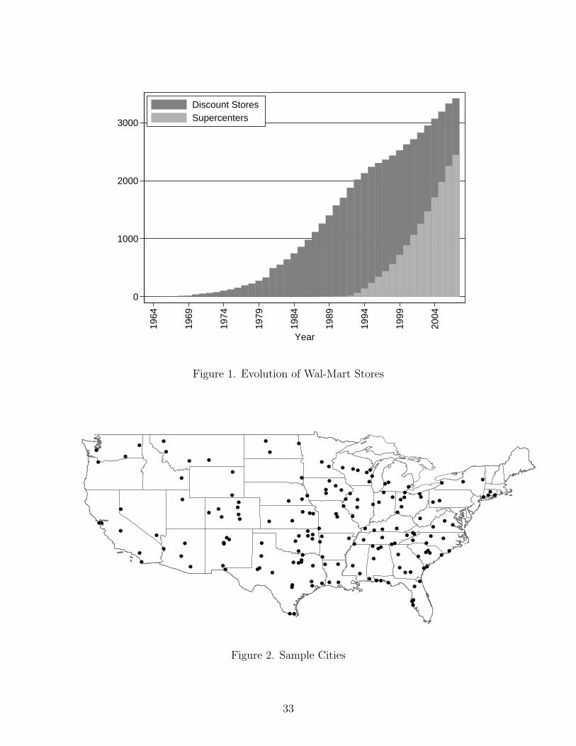
fast as Wal-Mart (Graff, 2006). Wal-Mart opened its first Supercenter as an experimental
format in 1988; today, more than 2,400 of Wal-Mart’s stores are Supercenters. Figure 1
shows the number of Wal-Mart stores and Supercenters up to 2004. Wal-Mart currently
accounts for 14% of Kraft and Kellogg’s sales, 16% of General Mills’ sales, and 11% of
Pepsi’s sales (Warner, 2006). Wal-Mart’s success is often attributed to its expert logistics
systems (Ellickson, 2006; Westerman, 2001) and its cost-conscious “corporate culture.” In
the retail sector as a whole, the productive gap between large national chains and single-unit
retailers is quite large (Foster, Haltiwanger, and Krizan, 2006) and it is conceivable that
food retailing exhibits even more asymmetries than the retail sector average.
Several recent studies have found that Wal-Mart charges lower prices than competitors.
For example, a 2002 UBS Warburg survey of 100 grocery and non-grocery items in 4–5
3
grocery stores in three markets with both Wal-Mart and non-Wal-Mart grocery stores found
that Wal-Mart’s prices were 17–39% lower than competitors’ prices (Currie and Jain, 2002).
? find a 30% premium at traditional supermarkets over superstores, mass merchandisers
and club stores (SMCs) for a similar array of products.
The causal impact Wal-Mart has on competitors’ prices has been less firmly established.
The UBS study, for example, finds that prices in Las Vegas, Houston and Tampa, which had
Wal-Mart Supercenters, were on average 13% lower than prices in Sacramento, which did
not have any Supercenters (Currie and Jain, 2002), but does not establish Wal-Mart’s causal
role in this difference. Basker (2005) uses a data set of all Wal-Mart’s store locations and
opening dates to estimate its effect on average prices of drugstore items such as shampoo and
toothpaste, but those prices are averaged over a number of surveyed establishments, which
may include Wal-Mart along with its competitors. As a result, Basker’s (2005) estimates
may confound Wal-Mart’s direct and indirect effects. Zhu, Singh, and Dukes (2005) analyze
the effect of entry of a Wal-Mart discount store, which does not sell groceries, on nearby
Dominick’s Finer Foods supermarkets using a case-study approach. But they focus on store
traffic and revenue, not prices. Similarly, Singh, Hansen, and Blattberg (2006) use a case
study to analyze the impact of a new Wal-Mart Supercenter on an incumbent chain grocery
store 2 miles away, and find an increase in the incumbent’s promotions (“sales”) and a decline
in quantities purchased, but no consistent pattern for prices at the competing supermarket.
In this paper, we estimate Wal-Mart’s causal effect on competitors’ grocery prices.
In related work, ? use data from AC Nielsen Homescan data which contain both prices
paid and quantities purchased for a large panel of consumers to estimate the competitive
effects of increased spending at SMCs on competitors prices. 3 They find that from 1998
to 2001, a period during which the market share of SMCs in their sample increased from
10.9% to 16.9% of grocery sales, average prices paid by consumers declined, on average,
by 3%. The effect varies from product to product. For a subset of items that overlap our
beef, lettuce, milk, potatoes and soda — their estimates imply that consumer prices fell by
2.6%. While ?’s (?) analysis focuses on the causal effects of shifting expenditure shares, due
to a combination of factors including entry, exit of competitors, and changes in consumers’
shopping venues or movements of relative prices, the focus of our paper is on the well-defined
causal impact of entry alone. 4
3 Data
Prices for 24 grocery items come from the American Chamber of Commerce Research Asso-
ciation (ACCRA). ACCRA, through local Chambers of Commerce, surveys up to 10 grocery
stores in the first week of each quarter in participating cities. Participating cities vary from
quarter to quarter, with some cities moving in and out of the sample frequently, while others
are included more regularly; 250–300 cities are surveyed each quarter during the sample
period. We obtained store-level prices from ACCRA for four points in time: July 2001, July
2002, July 2003 and July 2004. 5 We use a sample of 175 cities in the continental United
States that appear in the data in all four quarters; Figure 2 shows a map of their locations.
Table 1 provides summary statistics.
The stores surveyed include supermarket chains, “superstores” such as Wal-Mart, and
smaller grocers, but exclude membership clubs such as Sam’s Club or Costco. The number
of stores surveyed in any single market in a given survey period ranges from one (in 31
instances) to ten (in 905 instances); the mean, median and modal number of stores surveyed
in each market is five. 6 Approximately 14% of prices were collected at Wal-Mart stores.
7 The other stores in the sample are a representative mix of national, regional, and local
supermarkets.
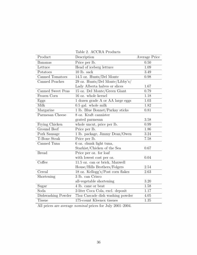
The products are listed in Table 2. They include dairy products (milk, eggs), meats
(chicken, sausage), produce (bananas, potatoes), canned goods (peaches, tuna), and miscel-
laneous items (sugar, dishwashing powder).
5
In each store, the price recorded is the lowest price available to all shoppers arriving at
the store. So, for example, discounts that require obtaining coupons in advance are never
factored in to price. Promotions that do not require coupons or for which coupons are
available in the store, and are redeemable on the spot, are factored in. In addition, lower
prices offered to customers with “frequent shopper” cards are used as long as the cards are
free and there is no waiting period for their use, conditions that are met by all supermarket
frequent-shopper programs with which we are familiar.
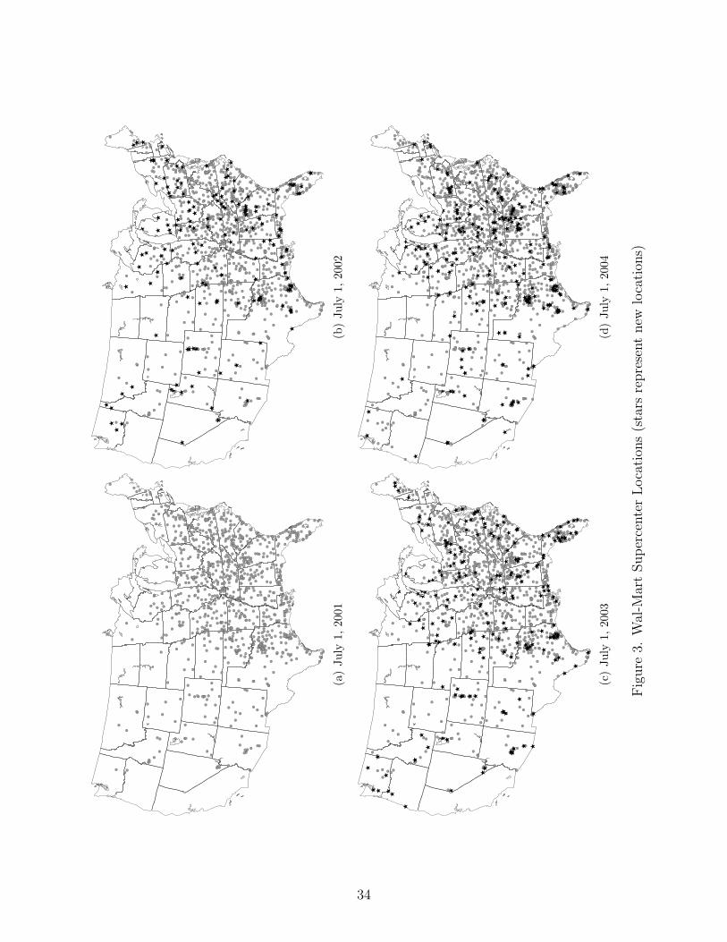
Wal-Mart provided the opening dates of all its U.S. stores, as well as dates of major
renovations, including conversions of “discount stores” to “Supercenters.” The initial opening
dates in the Wal-Mart administrative data are extremely accurate, but approximately a
quarter of the Supercenters that were converted from discount stores are missing conversion
dates in the file. We used press releases from Wal-Mart’s web site to obtain the conversion
dates for stores that were converted after March 2001. 8 Maps showing the locations of
Wal-Mart Supercenters as of July 1 of each year are shown as Figure 3; new Supercenters
since the previous July (for 2002–2004) are shown as stars.
Of the 175 sample cities, 23 had their first Supercenter open between July 2001 and July
2004. The number of Wal-Mart Supercenters increased in a total of 59 cities in the sample
during the study period; of these, 19 had more than one Supercenter added. 9
The locations and opening dates of Wal-Mart’s food Distribution Centers were obtained
from Tom Holmes, who compiled the data from various sources including ammonia permit
requests and subsidy information. Finally, we use the 2000 Census of Population to obtain
population size and 1999 median household income by city.
6
4 Methodology and Results
4.1 Cross-Sectional Estimates
We start by estimating the difference between Wal-Mart’s price and competitors prices in
markets that already include a Wal-Mart Supercenter. To do this, we calculate the average
non-Wal-Mart price as the unweighted average of log prices across all other surveyed retail
establishments, excluding Wal-Mart, for each product and city at each point in time, and
the average Wal-Mart price as the unweighted average of log prices across all Wal-Mart
Supercenters in the market, if there is more than one. Consistent with both popular percep-
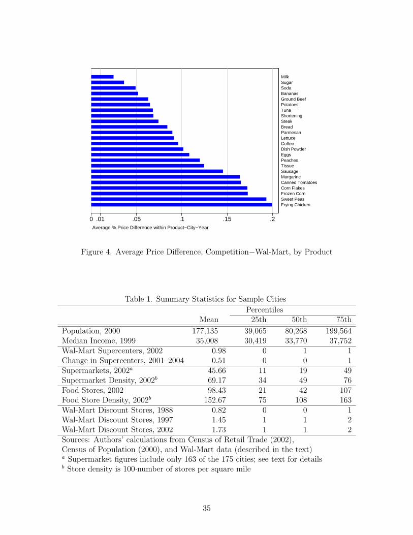
tion and previous studies, on average, Wal-Mart’s prices are 10.5% lower than competitors’
prices for these items. Figure 4 presents a graphical depiction of the average log difference
between Wal-Mart’s price and the non-Wal-Mart price in cities with at least one Wal-Mart
Supercenter by product. The differences range from 2.4% (milk) to 19.8% (frying chicken).
While these price differences are substantial and statistically different from zero for all
products, they are smaller than ones described by ?, who found an average price difference
of 27% between supercenters, mass merchandisers, and clubs (SMCs) on the one hand and
traditional supermarkets on the other. The most likely reason for the gap between our
estimates is data differences. The ACCRA data we use provide comparable prices for specific
items across stores, both within and across markets. The AC Nielsen Homescan data used
by ? attempt to capture the prices consumers pay for broader product categories, allowing
for substitution across products and outlet types. For example, ACCRA data specifically
exclude membership clubs, which use two-part tariff pricing (an annual membership fee,
and lower unit prices) and tend to sell larger packages which are not directly comparable
with other stores. Since clubs charge lower prices than other retailers, the Homescan SMC
prices are typically lower than Wal-Mart’s prices alone. Another difference is that ACCRA
products are very narrowly defined, specifying the package size and often the brand of the
item priced, whereas Homescan product categories are fairly wide and include products that
7
vary in brand, quality, and package sizes. Finally, ACCRA prices are actual prices collected
in a single week whereas the Homescan data used by ? are aggregated to the monthly
level, using quantity weights that reflect consumers’ product and intertemporal substitution
patterns.
For the remainder of the paper, we use pjkt to denote the average log price of product
k across non-Wal-Mart stores in market j at time t.
Because many studies have employed simple comparisons of prices in “Wal-Mart cities”
and “non-Wal-Mart cities” (e.g., Currie and Jain, 2002), our first regression is a simple cross-
section using price data for each year separately and treating the number of Wal-Mart stores
in the market as exogenous. For 2002, we estimate:
pjk,2002 = α+ θWMSCj,2002 +∑
k
φkproductk + xjβ + εjk (1)
where pjk,2002 is the average non-Wal-Mart log price of product k in city j in July 2002,
WMSCj,2002 is the number of Wal-Mart Supercenters in city j at the beginning of July
2002, and productk is a product indicator. The control variables in xj are log population
(from the 2000 Census) and log 1999 median household income (we also report estimates
from regressions omitting these controls). To account for correlation in the error term across
products within a city, standard errors are clustered by city. There are no time effects in
the model because it contains a single cross-section, and no city effects because they are
perfectly correlated with the Wal-Mart variable.
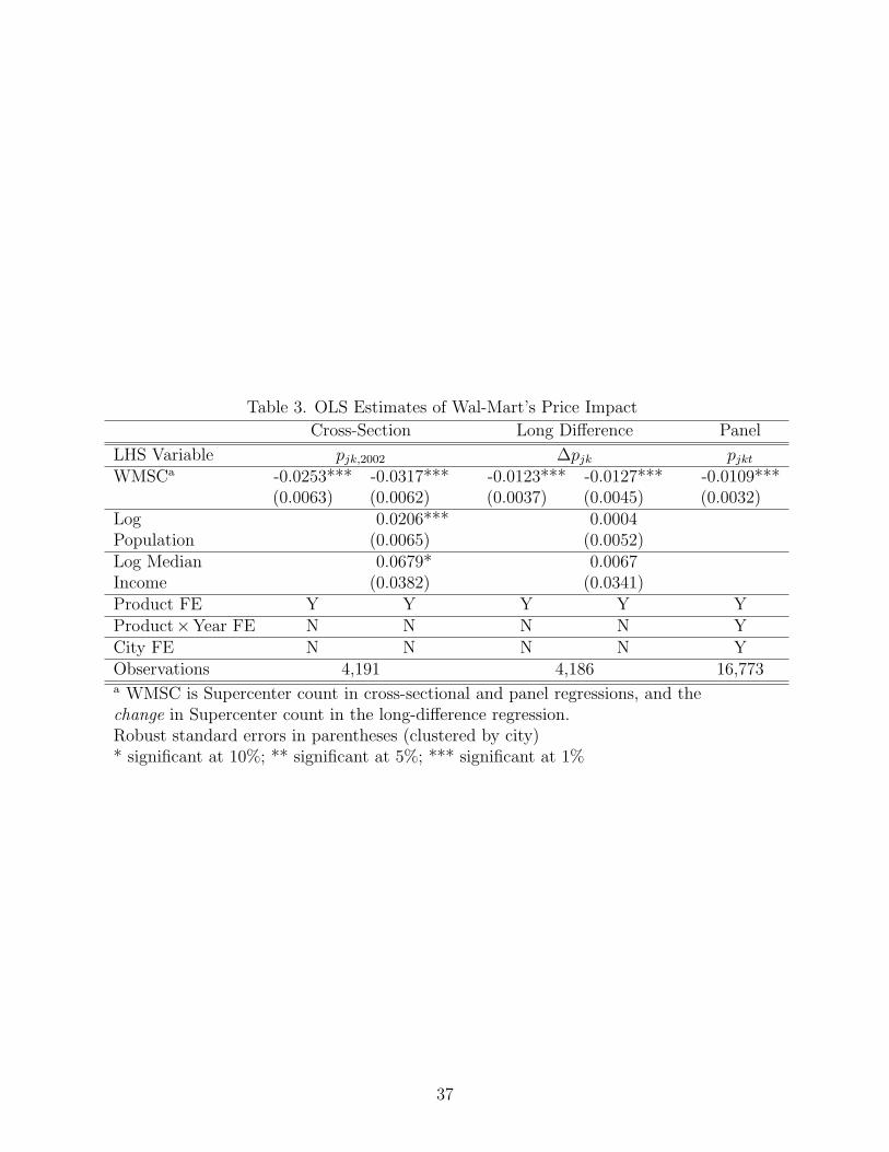
The results for the 2002 cross-section are shown in the first two columns of Table 3.
(We chose 2002 as an arbitrary mid-sample year. Results for other years, not shown, are
very similar.) In the first column we omit the control variables, which we add in the second
column. The estimates show that each Supercenter is correlated with competitors’ average
prices that are 2.5–3% lower, significantly different from zero at the 1% level. We also
estimate Equation (1) separately for each product, with all the control variables; the results
8
are shown in the first column of Table 4.
Using the number of Wal-Mart Supercenters as an explanatory variable allows us to
efficiently exploit the maximum amount of variation in the cross-sectional data. We have
experimented with two alternative specifications (not shown). First, we use an indicator
function, which equals 1 if there is at least one Supercenter in the city, to replace the
number of Wal-Mart Supercenters. In July 2002, 108 of our 175 cities had at least one
Supercenter. (That number increased from 98 to 121 between July 2001 and July 2004.)
The indicator function misses, however, the variation in the number of Supercenters among
these cities; on average, a city with one or more Supercenters in 2002 had 1.6 such stores,
and the standard deviation was 0.9. Estimates using the indicator function imply that price
reductions by competing grocery stores are larger than those that use the number of stores,
averaging 5.5% per Supercenter (standard errors are also larger). 10 When we allow the
effect of the first Supercenter to differ from the effect of additional Supercenters, we find
that the first Supercenter reduces prices by 8–9% and additional Supercenters have marginal
effects of 2–3%, all statistically significant at the 1% level.
Unfortunately, the cross-sectional estimates cannot be interpreted causally due to omit-
ted variable bias. Wal-Mart stores are not assigned randomly to sample cities, and factors
that affect the number of Wal-Mart stores in a market are likely to be correlated with the
error term in these price regressions. Because Wal-Mart caters to low-income consumers,
and because it has traditionally operated in low-cost areas in the South and Midwest, we
expect this bias to drive the estimated coefficients downward (away from zero). We next
turn to some OLS specifications that are better designed to address this issue. We return to
the cross-sectional specification in Appendix A where we consider two instrumental variables
methods that attempt to address the omitted-variable bias.
9
4.2 Long Difference Estimates
As a better alternative to the cross sectional model, we also estimate a long-difference re-
gression,
∆pjk = α+ θ∆WMSCj +∑
k
φkproductk + xjβ + εjk (2)
which has the change in log average non-Wal-Mart prices of product k in city j between July
2001 and July 2004 on the LHS, and the change in the number of Wal-Mart Supercenters
in city j over this time period, along with product fixed effects on the RHS. This specifi-
cation has the advantage that time-invariant characteristics of the market are removed by
the differencing, removing many possible omitted variables. Estimates obtained from this
specification are valid if the number of new Wal-Mart Supercenters over this period is un-
correlated with the error term. An implicit assumption in these regressions is that only the
entry of Wal-Mart, and not the exact timing of this entry — as long as it occurs within the
3-year window from July 2001 to July 2004 — matters.
Results are shown in the third and fourth columns of Table 3. Estimates of price reduc-
tions are around 1.2% and are significantly different from zero at the 1% level. Combining
this indirect effect of Wal-Mart Supercenter entry on the prices of competing supermarkets
with the post-entry price difference of 10.5% calculated above, we estimate that compet-
ing grocery stores do cut prices when Wal-Mart enters their market, but only by 1/10th of
their initial (pre-entry) price premium over Wal-Mart. The second column of Table 4 shows
product-by-product estimates of Equation (2), with all the control variables.
This estimate of the indirect effect is smaller by 50% or more than the cross-sectional
estimates, consistent with our concern that the cross-sectional estimates attribute too much
of the differences across cities to Wal-Mart. As a specification check, we also estimated this
model with the initial (2001) log price on the right-hand side, along with the other control
variables; coefficient estimates are very similar to those shown.
10
4.3 Panel Estimates
Our third and preferred OLS specification is a panel with market fixed effects. Like the long-
difference regression, the panel regression controls for all unobserved time-invariant factors
that influence market demand. In addition, while the long-difference specification does not
use information on the exact timing of Wal-Mart’s entry or the timing of price responses, the
panel specification is more efficient because it uses all available information. We estimate
pjkt = α+ θWMSCjt +∑
j
γjcityj +∑kt
δktyeartproductk + εjkt (3)
where pjkt is the average non-Wal-Mart log price of product k in city j at time t, WMSCjt
is the number of Wal-Mart Supercenters in city j at time t, cityj is a city indicator to capture
cost and price differences across cities for any reason other than Wal-Mart’s entry, yeart is a
year indicator and productk is a product indicator; their interaction is intended to capture
overall cost differences and changes at the product level. 11 To account for correlation in
the error term across products and over time within a city, standard errors are clustered by
city.
OLS estimates of Equation (3) are interpretable as causal effects of Wal-Mart’s entry
and expansion if and only if, conditional on Wal-Mart’s entry or expansion into market j
over the period July 2001–July 2004, the exact timing (year) of entry is uncorrelated with
the εjkt. This is a relatively weak condition: time-invariant city characteristics are captured
with the city fixed effects and the panel is short enough that there are unlikely to be many
large changes in city characteristics. This is effectively a difference-in-difference estimator.
Results are shown in the last column of Table 3. The effect of a Wal-Mart Supercenter
is now estimated to be a price reduction of approximately 1.1% among other grocery stores.
This effect is identified using 90 Supercenter openings in the sample cities over the period
studied, distributed roughly equally across time (26 between July 2001 and July 2002, 34
the following year, and 30 in the final year). This estimate is very slightly smaller — and
11
slightly more precise — than the long-difference estimates reported earlier. The 1.1% price
reduction by competing grocery stores is modest compared to Wal-Mart’s direct effect —
prices that are 10% lower — suggesting the benefits from Wal-Mart Supercenters accrue
mostly to consumers who shop there, while consumers who do not modify their shopping
habits benefit little.
We prefer using the number of Supercenters on the LHS to other specifications because
it uses all available information, and efficiently exploits the most variation in the data. If
we replace this variable with an indicator variable which equals 1 if there is a Supercenter
in the market, we identify the Supercenter effect using only the 23 initial entries into a
market (19 of them in the first two years), compared with the 90 openings used above.
In this specification, the estimated effect of each Supercenter entry (not shown) increases
to 1.65%, but standard errors are 2–3 times larger than in our main specification. 12 We
also experimented with a specification in which we allow for the first Supercenter to have a
different effect from subsequent ones. The results (not shown) suggest the effects of the first
and later Supercenters are almost identical, and statistically indistinguishable, at −1.2% and
−1.1%, respectively. The first of these is not statistically different from zero but the second
is significant at the 1% level.
These estimates of 1–1.2% price reductions per Supercenter mask larger average price
reductions over our sample period. The 59 cities in our sample in which the number of
Wal-Mart Supercenters increased over the three-year period July 2001–July 2004 averaged
an increase of 1.5 Supercenters over this time. Our estimates therefore imply that, in the
average city with Supercenter entry or expansion grocery prices at competing supermarkets
fell by 1.5–1.8% over this three-year period.
The third column of Table 4 shows estimates of Equation (3) for each product separately.
Effects range from price reductions of 3.65% for margarine to price increases of 0.65% for
soda, with twenty two of the 24 coefficients negative. Point estimates are statistically differ-
ent from zero at the 5% level (and negative) for seven products: bananas, lettuce, canned
12
tomatoes, margarine, frying chicken, dish washing powder, and tissues (estimates for sausage
are significant at the 10% level). Neither of the positive coefficients is significantly different
from zero.
The panel estimates provide the cleanest identification and the smallest coefficient esti-
mates (in absolute terms) among the OLS specifications. Estimates of the marginal effect of
a new Wal-Mart Supercenter fall from approximately 3% in the cross-sectional regression to
1.2% in the long-difference regression and to 1.1% in the panel regression. These differences
are driven by the assumptions required for causal interpretation. The cross-sectional regres-
sions assume that the locations of Wal-Mart stores are not correlated with anything that
influences price. Long-difference estimates assume that this is true only of the new locations
over the period studied and that the timing of entry does not matter for the price impact.
Panel estimates assume that the choice to enter a particular market during this 3-year pe-
riod may be endogenous, but conditional on entry, the exact timing is uncorrelated with
other determinants of prices. The fact that the panel estimates, which impose the weakest
conditions on causal interpretation, provide the smallest point estimates is consistent with
the common perception that Wal-Mart tends to open stores in low-price locations.
There is another difference between the cross-sectional, long-difference, and panel OLS
estimates, however, that has to do with the time horizon over which Wal-Mart’s Supercenters
can affect the competition. The panel regression has the shortest horizon, in the sense that
it only reflects short-run effects of the change in the number of Supercenters on competitors’
prices. The long-difference regression allows the effects to accumulate over the study period.
Because entry of Supercenters in our sample cities is spread approximately uniformly over
the 3-period, the long-difference estimates represent an average of the 1-year, 2-year, and
3-year price changes due to competition with a Supercenter. That point estimates in the
long-difference specification are slightly larger than those in the panel specification suggests
that the medium-run (2-3 year) effects of Supercenter competition may be slightly larger
than the short-run effects. The cross-sectional estimates take this a step further. Several of
13
the Supercenters in our sample, such as the ones in Augusta, GA, and Jefferson City, MO,
are among the very first Supercenters to open in the late 1980s and 1990. Others opened
just before, or during, the sample period. As a result, in addition to the omitted-variable
bias, the cross-sectional confound short-, medium-, and long-run effects.
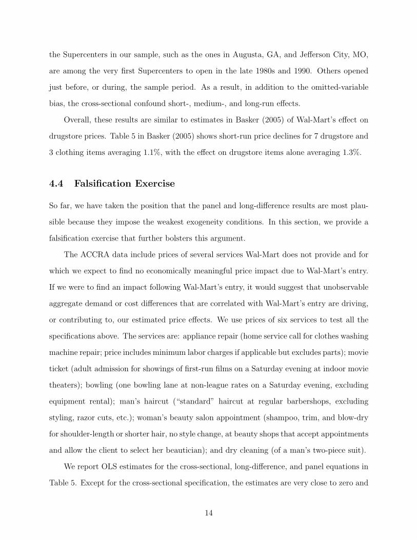
Overall, these results are similar to estimates in Basker (2005) of Wal-Mart’s effect on
drugstore prices. Table 5 in Basker (2005) shows short-run price declines for 7 drugstore and
3 clothing items averaging 1.1%, with the effect on drugstore items alone averaging 1.3%.
4.4 Falsification Exercise
So far, we have taken the position that the panel and long-difference results are most plau-
sible because they impose the weakest exogeneity conditions. In this section, we provide a
falsification exercise that further bolsters this argument.
The ACCRA data include prices of several services Wal-Mart does not provide and for
which we expect to find no economically meaningful price impact due to Wal-Mart’s entry.
If we were to find an impact following Wal-Mart’s entry, it would suggest that unobservable
aggregate demand or cost differences that are correlated with Wal-Mart’s entry are driving,
or contributing to, our estimated price effects. We use prices of six services to test all the
specifications above. The services are: appliance repair (home service call for clothes washing
machine repair; price includes minimum labor charges if applicable but excludes parts); movie
ticket (adult admission for showings of first-run films on a Saturday evening at indoor movie
theaters); bowling (one bowling lane at non-league rates on a Saturday evening, excluding
equipment rental); man’s haircut (“standard” haircut at regular barbershops, excluding
styling, razor cuts, etc.); woman’s beauty salon appointment (shampoo, trim, and blow-dry
for shoulder-length or shorter hair, no style change, at beauty shops that accept appointments
and allow the client to select her beautician); and dry cleaning (of a man’s two-piece suit).
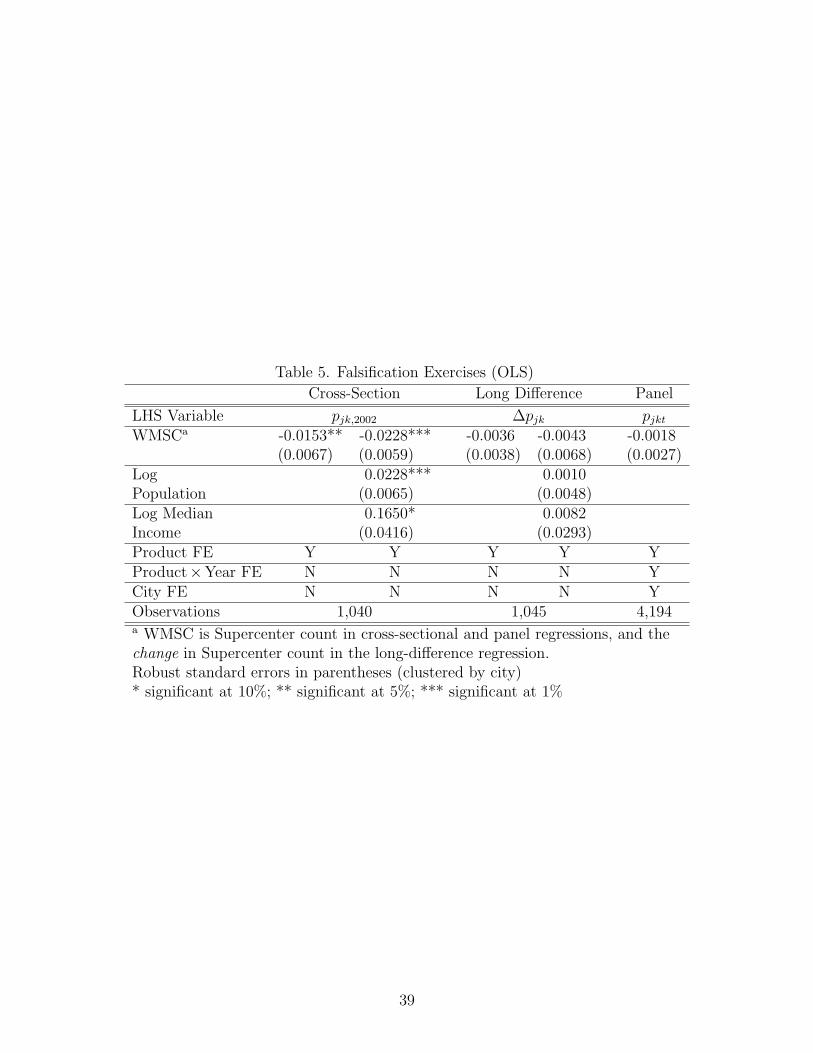
We report OLS estimates for the cross-sectional, long-difference, and panel equations in
Table 5. Except for the cross-sectional specification, the estimates are very close to zero and
14
statistically insignificant despite tight confidence intervals. The cross-sectional estimates are
statistically different from zero, consistent with our concern that differences in the number of
Wal-Mart stores across cities cannot be treated as exogenous, and unobserved demand and
cost differences across markets are in part driving the estimates. These estimates confirm our
concern that endogeneity increases the estimated effect of Wal-Mart’s Supercenters in the
cross-sectional regressions, because Wal-Mart’s traditional markets have been in low-income,
low-cost cities. The cross-sectional estimates are only about 1 percentage point smaller (in
absolute terms) than the corresponding estimates for grocery products shown in Table 3.
One way to interpret this 1% figure is as a difference-in-difference estimate, where the two
“difference” dimensions are the number of Wal-Mart stores in a market and whether the
product is sold by Wal-Mart, and unobservable city-specific effects are differenced out. The
identifying assumption is that unobserved shocks to cost and demand affect grocery and
service prices equally. The difference of 1% is, in fact, almost exactly the estimate we get
in the difference-in-difference panel regression in the last column of Table 3, in which the
difference dimensions are the number of Wal-Mart stores in a market and time.
The long-difference and panel point estimates are very small and statistically insignifi-
cant, adding to our confidence in these specifications. The panel estimates are particularly
small, at less than one fifth of one percent. We conclude from these falsification exercises that
the indirect effect of Wal-Mart entry on competitors’ prices, estimated in the long differences
and panel specifications, are true competitive effects. They do not appear to be driven by
correlation with unobserved aggregate or city-specific demand shocks. Effectively, our panel
estimate is also the difference-in-difference-in-difference estimate, which exploits differences
in three dimensions: the number of Wal-Mart stores in a market, grocery products sold at
Wal-Mart versus services not provided at Wal-Mart, and time.
15
5 Heterogeneous Responses
While the average price reduction in response to Wal-Mart’s entry is a modest 1.1%, the
impact is likely to be heterogeneous across competitors of different sizes and types. We
expect competitors whose clientele is most similar to Wal-Mart’s — for which the cross-
price elasticity of substitution is high — to make the largest price reductions; competitors
that are differentiated in selection and other amenities (service, location, etc.) should react
the least. Relatedly, we expect the overall competitive environment in each city to affect
the price response: markets in which prices are already highly competitive should see the
smallest additional price reductions in response to Wal-Mart. In this section, we test these
hypotheses and also explore how price reactions vary with market demographics.
There has been some speculation in the press that the supermarket chains most im-
pacted by a Wal-Mart Supercenter’s entry are those with the largest revenue stakes in the
industry (see, e.g., Callahan and Zimmerman, 2003). The “Big Three” supermarket chains
(Albertson’s, Kroger, and Safeway) dwarf other conventional supermarket chains; over the
period of this study they controlled, collectively, approximately 30% of all supermarket sales.
13 They are also disproportionately unionized. Their unionization rates range from 60–80%,
a factor that has driven up their costs and may leave them less leeway for price competition
(Albertson’s, Inc., 2004; Kroger, 2006; Safeway Inc., various years). 14
Wal-Mart’s efficient distribution system in traditional retailing gives it a cost advantage
over other retailers. In addition, Wal-Mart stores provide minimal service to keep costs low.
Although we do not have cost and inventory data to confirm this empirically for grocery
retailing, there is some evidence that they carry few brands within each product class (see
Dukes, Geylani, and Srinivasan, forthcoming, for a discussion), which further reduces costs
through economies of scale in purchasing. Given Wal-Mart’s strategy of charging prices sub-
stantially lower than competitors (10% lower by our calculations) traditional supermarkets
need to respond to Wal-Mart Supercenter entry in some way.
A competitor facing new entry by Wal-Mart has two possible approaches. 15 First, it
16
may attempt to reduce prices, either by lowering costs (for example by increasing efficiency,
cutting back on service levels, or reducing the quality of the groceries sold) or by lowering
profit margins, to compete head-on with Wal-Mart on price. This may be the only option
for a chain that has firmly positioned itself in the marketplace as a low-end low-price chain
targeting price-elastic consumers. The other option available to a full-service supermarket
is to shift its focus, at least in part, away from the most price-sensitive consumers (whose
“defection” to Wal-Mart is assumed to be a lost cause) and position itself more firmly in
the higher-end market that caters to less price-elastic consumers. Inelastic consumers put
greater value on increased quality of products, improved service, better selection, convenience
of location, and the overall shopping experience. 16 For example, a chain may adjust its
marketing focus, introduce a “farmer’s market” format, include tasting stations, or make
available a selection of high-end specialty foods like organic produce. 17
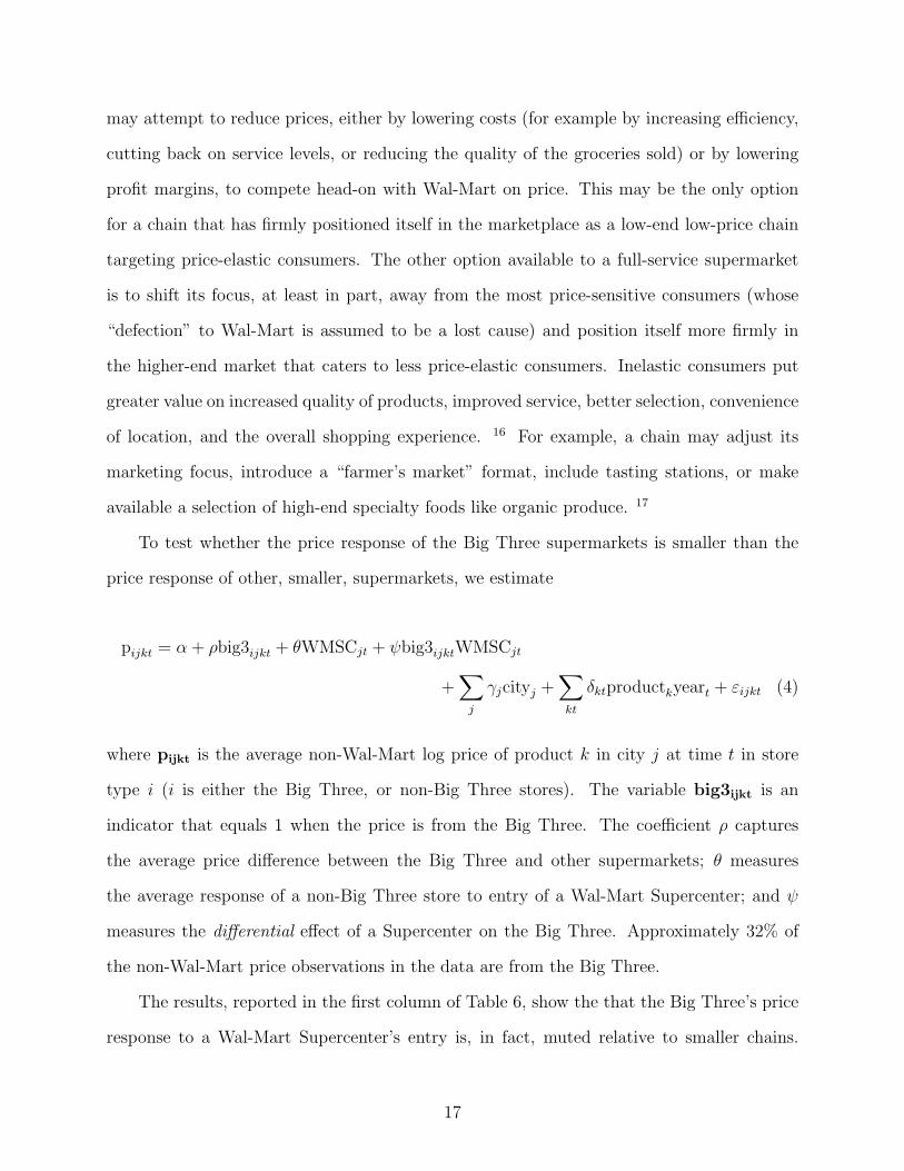
To test whether the price response of the Big Three supermarkets is smaller than the
price response of other, smaller, supermarkets, we estimate
pijkt = α+ ρbig3ijkt + θWMSCjt + ψbig3ijktWMSCjt
+∑
j
γjcityj +∑kt
δktproductkyeart + εijkt (4)
where pijkt is the average non-Wal-Mart log price of product k in city j at time t in store
type i (i is either the Big Three, or non-Big Three stores). The variable big3ijkt is an
indicator that equals 1 when the price is from the Big Three. The coefficient ρ captures
the average price difference between the Big Three and other supermarkets; θ measures
the average response of a non-Big Three store to entry of a Wal-Mart Supercenter; and ψ
measures the differential effect of a Supercenter on the Big Three. Approximately 32% of
the non-Wal-Mart price observations in the data are from the Big Three.
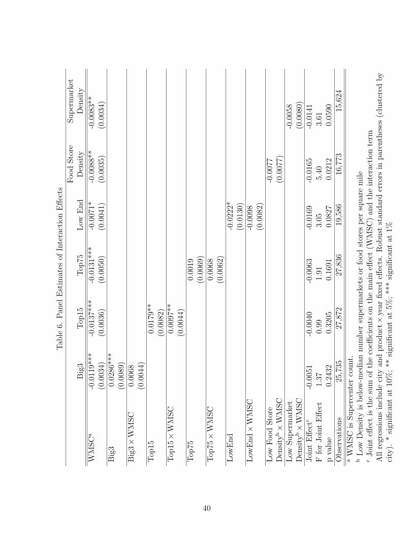
The results, reported in the first column of Table 6, show the that the Big Three’s price
response to a Wal-Mart Supercenter’s entry is, in fact, muted relative to smaller chains.
17
Consistent with higher costs, the Big Three supermarkets in markets without a Wal-Mart
Supercenter charge a statistically-significant 2.86% premium over smaller chains. In addition,
Wal-Mart’s entry impacts the Big Three less than other supermarkets. While the smaller
chains lower prices, on average, by 1.2%, the Big Three stores lower their prices by only
a statistically insignificant 0.51%. As a result, the price difference between the Big Three
and other supermarkets increases by 0.68 percentage points with each Wal-Mart Supercenter
entry. Thus, at least in the price dimension, the large chains that make up the Big Three
are least likely to react.
Given their size and market dominance, the distinction between the Big Three and
all smaller chains is the most natural, but there are other measures of size as well. To
cut the data differently we define a large chain as one that has been consistently ranked
among the top fifteen firms in Supermarket News’s list of the Top 75 North American Food
Retailers (Supermarket News, various years). There are seven such firms in our data: the
Big Three plus Ahold, Supervalu, Winn-Dixie, and Meijer; collectively, they account for 43%
of price observations. The results in the second column show that the Top-15 supermarkets’
prices in markets with no Wal-Mart Supercenters are, on average, 1.8% higher than other
supermarkets’ prices. After a Supercenter entry, Top-15 prices fall by only a statistically-
insignificant 0.4% in response to Wal-Mart’s entry, whereas other supermarkets’ prices fall
by nearly 1.4%. The gap between prices at the Top-15 chains and the other chains increases
by nearly 1% with each Supercenter. When we include the Big Three and the other Top-15
chains separately (not shown) we find that almost all of the price difference comes from the
Big Three.
Expanding the group of large chains to include all Top-75 retailers — a total of 66 chains
consistently ranked in the Top 75 North American Food Retailers by Supermarket News over
this period — confirms the pattern. (These firms account for 63% of all price observations
in the data.) In markets with no Supercenter, Top-75 firms charge only a statistically-
insignificant 0.2% premium over other chains, but increase their premium by approximately
18
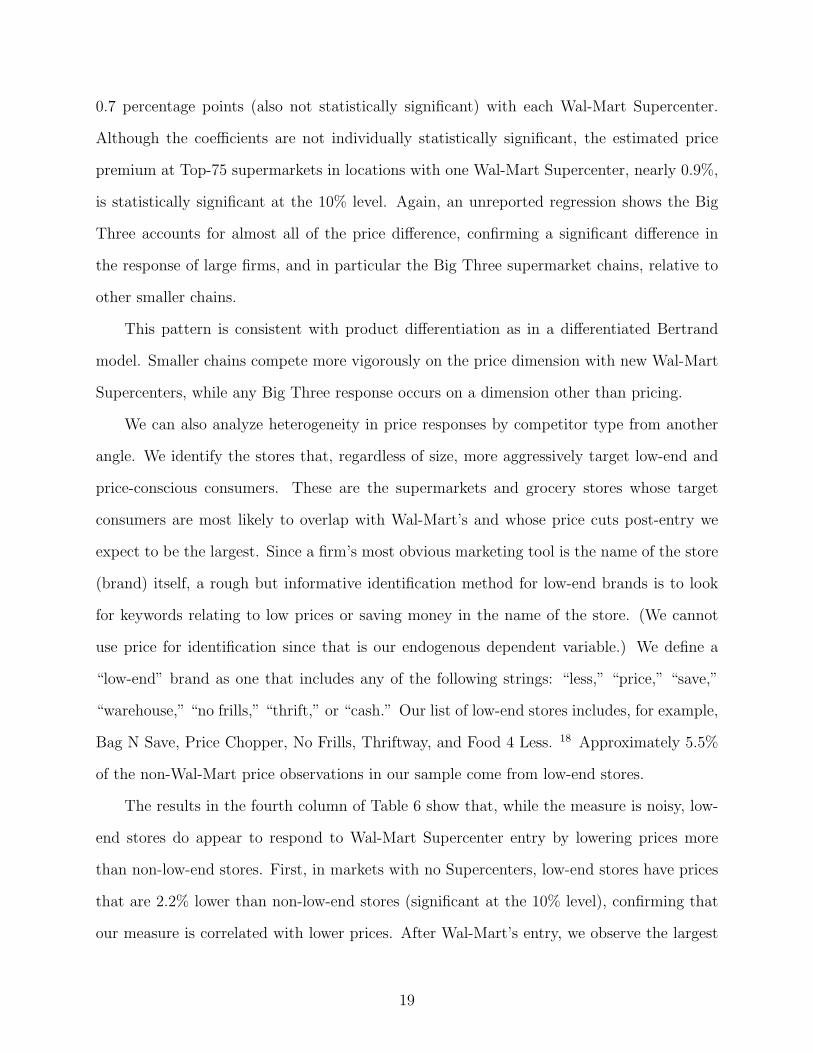
0.7 percentage points (also not statistically significant) with each Wal-Mart Supercenter.
Although the coefficients are not individually statistically significant, the estimated price
premium at Top-75 supermarkets in locations with one Wal-Mart Supercenter, nearly 0.9%,
is statistically significant at the 10% level. Again, an unreported regression shows the Big
Three accounts for almost all of the price difference, confirming a significant difference in
the response of large firms, and in particular the Big Three supermarket chains, relative to
other smaller chains.
This pattern is consistent with product differentiation as in a differentiated Bertrand
model. Smaller chains compete more vigorously on the price dimension with new Wal-Mart
Supercenters, while any Big Three response occurs on a dimension other than pricing.
We can also analyze heterogeneity in price responses by competitor type from another
angle. We identify the stores that, regardless of size, more aggressively target low-end and
price-conscious consumers. These are the supermarkets and grocery stores whose target
consumers are most likely to overlap with Wal-Mart’s and whose price cuts post-entry we
expect to be the largest. Since a firm’s most obvious marketing tool is the name of the store
(brand) itself, a rough but informative identification method for low-end brands is to look
for keywords relating to low prices or saving money in the name of the store. (We cannot
use price for identification since that is our endogenous dependent variable.) We define a
“low-end” brand as one that includes any of the following strings: “less,” “price,” “save,”
“warehouse,” “no frills,” “thrift,” or “cash.” Our list of low-end stores includes, for example,
Bag N Save, Price Chopper, No Frills, Thriftway, and Food 4 Less. 18 Approximately 5.5%
of the non-Wal-Mart price observations in our sample come from low-end stores.
The results in the fourth column of Table 6 show that, while the measure is noisy, low-
end stores do appear to respond to Wal-Mart Supercenter entry by lowering prices more
than non-low-end stores. First, in markets with no Supercenters, low-end stores have prices
that are 2.2% lower than non-low-end stores (significant at the 10% level), confirming that
our measure is correlated with lower prices. After Wal-Mart’s entry, we observe the largest
19
reductions in low-end stores’ prices. Whereas the average non-low-end store lowers its price
by only 0.7% in response to Wal-Mart’s entry, the typical low-end store lowers its price by
1.7%. Although the difference falls shy of statistical significance at conventional levels it is
economically large, increasing the price discount at low-end stores (relative to non-low-end
stores) by a percentage point with each Wal-Mart Supercenter. This pattern is consistent
with the hypothesis that Wal-Mart’s impact on prices is greatest at chains that compete for
the same low-end, price elastic consumers. 19 The finding is especially interesting because of
the likelihood that low-end stores start out with slimmer profit margins, which limits their
ability to cut prices further. This effect, however, is evidently dominated by the fact that
Wal-Mart appeals to many of the same consumers. 20
Another dimension of differentiation we can measure is the ease of consumer access
to Supercenters vs. traditional supermarkets. The more densely are supermarkets and
Supercenters located the lower the degree of spatial differentiation and, ceteris paribus, the
tighter price competition. One might expect this effect should lead to greater price cuts
by competitors in response to a Wal-Mart Supercenter entry. However, if stores in densely-
competitive markets work harder to differentiate themselves on other dimensions and operate
with profit margins that are already razor thin, they may not have the ability, or the need,
to cut prices further. They would need to differentiate themselves in other ways.
To test for the effect of supermarket density on the impact of Wal-Mart Supercenter
entry, we use data from the 2002 Census of Retail Trade to obtain a measure of the number
of food and beverage stores (NAICS 445) in each city, a category that includes grocery
stores and supermarkets, convenience stores, specialty food stores (such as meat markets and
vegetable markets, and beer, wine, and liquor stores. We calculate the food-store density
by dividing the number of food stores by the city’s area, in square miles, obtained from the
2000 County and City Data Book. 21 For a subset of our sample (163 of the 175 cities) we
can also calculate the supermarket density (NAICS 44511), which we use as a robustness
check. For the median city in our sample, the number of supermarkets per square mile is
20
0.49 and the number of food and beverage stores per square mile is 1.08. (The means are
0.69 and 1.53 respectively.)
The density variables vary by city but not over time, so they are perfectly colinear with
the city fixed effects in the regressions. However, we can identify the differential effect of
Wal-Mart in low- vs. high-density markets by estimating
pjkt = α+ θWMSCjt + ηLowDensityjWMSCjt
+∑
j
γjcityj +∑kt
δktproductkyeart + εjkt (5)
where LowDensityj is 1 if city j’s food store (or supermarket) density is below the median
in the sample, and 0 otherwise. Now, the coefficient θ captures the effect of a Supercenter
entry on average prices in high food-store density markets, and the coefficient η captures the
additional impact of Wal-Mart on prices in low-density markets.
These results are shown in the last two columns of Table 6. Using the impact of Wal-
Mart’s entry on cities with a high food store density is estimated at a statistically-significant
0.9%; the impact on cities with a low supermarket density is a statistically significant 1.65%.
Both effects are significantly different from zero at the 5% level. The difference-in-difference
is not statistically significant, but the sign is consistent with a larger impact of Wal-Mart
in less-competitive and higher-margin markets, than in markets where much of the profit
margins have already been competed away.
For completeness, we also experimented with a variety of other specifications, not shown,
examining differential effects by region, by city population, and by average income and
poverty rates. We found that the effect of Wal-Mart Supercenters is slightly larger in the
South than in other regions, but was neither economically nor statistically different in small
vs. large cities or in high-income (low-poverty) vs. low-income (high-poverty) cities.
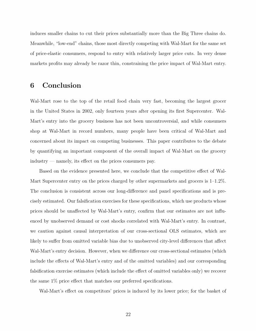
Overall, we conclude that the impact of Wal-Mart Supercenter entry on competitor
prices, while averaging 1.1%, is not uniformly distributed across its competitors. Wal-Mart
21
induces smaller chains to cut their prices substantially more than the Big Three chains do.
Meanwhile, “low-end” chains, those most directly competing with Wal-Mart for the same set
of price-elastic consumers, respond to entry with relatively larger price cuts. In very dense
markets profits may already be razor thin, constraining the price impact of Wal-Mart entry.
6 Conclusion
Wal-Mart rose to the top of the retail food chain very fast, becoming the largest grocer
in the United States in 2002, only fourteen years after opening its first Supercenter. Wal-
Mart’s entry into the grocery business has not been uncontroversial, and while consumers
shop at Wal-Mart in record numbers, many people have been critical of Wal-Mart and
concerned about its impact on competing businesses. This paper contributes to the debate
by quantifying an important component of the overall impact of Wal-Mart on the grocery
industry — namely, its effect on the prices consumers pay.
Based on the evidence presented here, we conclude that the competitive effect of Wal-
Mart Supercenter entry on the prices charged by other supermarkets and grocers is 1–1.2%.
The conclusion is consistent across our long-difference and panel specifications and is pre-
cisely estimated. Our falsification exercises for these specifications, which use products whose
prices should be unaffected by Wal-Mart’s entry, confirm that our estimates are not influ-
enced by unobserved demand or cost shocks correlated with Wal-Mart’s entry. In contrast,
we caution against causal interpretation of our cross-sectional OLS estimates, which are
likely to suffer from omitted variable bias due to unobserved city-level differences that affect
Wal-Mart’s entry decision. However, when we difference our cross-sectional estimates (which
include the effects of Wal-Mart’s entry and of the omitted variables) and our corresponding
falsification exercise estimates (which include the effect of omitted variables only) we recover
the same 1% price effect that matches our preferred specifications.
Wal-Mart’s effect on competitors’ prices is induced by its lower price; for the basket of
22
food items in our study, Wal-Mart’s prices are about 10% lower than its competitors. Com-
petitors’ responses vary with their degree of differentiation from Wal-Mart. At one extreme,
the largest supermarket chains — Kroger, Albertson’s, and Safeway — reduce their prices
in response to Wal-Mart’s entry by less than half as much as its smaller competitors. At the
opposite extreme, low-end grocery stores which compete for the same high-elasticity con-
sumers by setting low prices, rather than providing high levels of service or other amenities,
lower their prices by twice as much as mainline supermarkets.
There are many potential dimensions along which competitors may respond to Wal-
Mart’s entry. In addition to short-run price adjustments, Wal-Mart’s entry may also change
the quantities or mix of products sold at competing supermarkets, which could have impli-
cations for long run prices. In the long run, competing supermarkets may contract or even
exit, causing prices to rise (due to less competition) or fall (due to a shift in the average
efficiency in firms). Potential entry by Wal-Mart, rather than actual entry, may also have an
effect if markets are contestable and incumbents suppress their prices to deter entry. This
paper addresses the causal effect of one of the most important and immediate effects, that
of short- and medium-run price responses. The large direct price effect we find demonstrates
that consumers who shop at Wal-Mart receive a sizeable price benefit, while the indirect
price effects are quite small, especially for shoppers at the Big Three supermarkets.
23
A Instrumental Variables
While we are comfortable with the weak exogeneity assumptions in the long-differences
and panel regressions, omitted-variable bias in the cross-sectional analysis prevents us from
making a causal interpretation of θ, the coefficient estimate from Equation (1). Our goal
in this section is to examine two instrumental-variables methods that might alleviate this
problem in the cross-sectional analysis. 22
Wal-Mart supplies its stores primarily through several dozen Distribution Centers (DCs)
around the country. As of July 2001, only 20 DCs dealt with groceries; by July 2004, twelve
more opened. According to Wal-Mart Watch, the median DC serves about 90 stores within
a 250 mile radius. If it is cheaper for Wal-Mart to supply markets closer to DCs, we should
observe more Supercenters in these markets. This logic leads us to use each market’s distance
to the nearest food DC to instrument for the number of Supercenters. However, conditional
on opening a Supercenter in a market, distance from the nearest food DC could also affect
the store’s costs and therefore prices, and thus the instrument may still be correlated with
the error term in Equation (1). A second problem is that Wal-Mart determines the locations
of its Supercenters and DCs simultaneously (see Holmes, 2008). Even though each DC serves
many stores, so that any one market has a minimal effect on the location of a DC, market
characteristics tend to be spatially correlated, which can exacerbate the endogenous element
in the DC location decision.
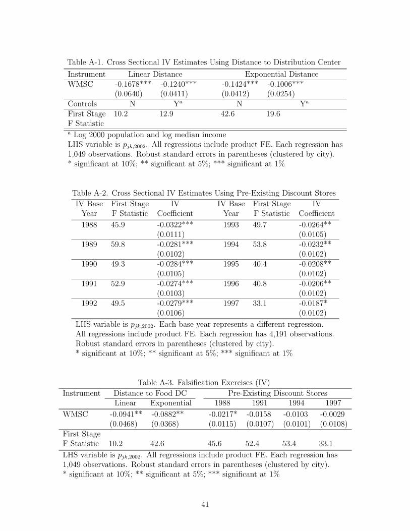
Table A-1 reports results using both linear distance to the nearest DC as the instrument,
as well as using exponential distance. 23 First-stage F statistics are in the range of 10 − 20
(except for one which has an F statistic of 42). Second-stage estimates are 3–5 times larger in
absolute value than the cross-sectional OLS estimates from Table 3, which were themselves
larger than the more-plausible panel and long-difference estimates. The IV estimates suggest
a price impact of 12–17% per Supercenter, more than 10 times our other estimates. These
numbers are implausible in light of the fact that grocery stores’ gross margins average below
30% (U.S. Census Bureau, 2006).
24
We conclude from this exercise that the instrument is not valid for our purpose. One
must be cautious about distance-based instruments in this context, because of spatial corre-
lation and the potential for a direct effect of distance on price. In this case these problems
exacerbate the selection problem instead of correcting for it. 24
Many of Wal-Mart’s Supercenters are conversions from pre-existing discount stores. One
reason for this is that such expansion is cheaper than de novo entry into a market. We exploit
this fact by using the number of pre-existing discount stores in a market to instrument for
Supercenter entry. The instrument is valid if the number of pre-existing discount stores is
uncorrelated with unobservable characteristics of the market that also affect competitors’
grocery prices, before and after Wal-Mart’s (potential) entry into the grocery market. To
minimize such potential correlations we use the number of Wal-Mart discount stores in a
relatively early time period, before Wal-Mart’s Supercenter format became widespread. We
report estimates using base years ranging from 1988 to 1997.
Table A-2 shows IV estimates for Equation (1). For each base year, we show the first-
stage F statistic and the estimated second-stage (IV) coefficient. In each case, the first-
stage results are strong and significant, with F statistics ranging from 30–50. The first-stage
coefficients (not reported) are positive and range from 0.5 to 0.6. IV estimates of competitors’
response range from 2–3% price reductions, falling as the base year increases. Interestingly,
F statistics are highest for the early base years: the number of discount stores in 1988 is a
better predictor of Supercenters in 2002 than the number of discount stores in 1997. This
is probably because many discount stores were converted to Supercenters between 1988 and
1997, so a location that still has many pure discount stores in 1997 is likely to be a relatively
bad location for a Supercenter. At the same time, the early base years also yield coefficient
estimates that are larger in absolute value than the OLS estimates, suggesting that the
same selection concerns that apply to Supercenters in 2002 may also apply to the choice of
locations of discount stores in earlier years. This implies that the number of discount stores
in later base years, 1997 in particular, may be the most reliable instrument.
25
Table A-3 repeats the falsification exercise from Section 4.4 for the cross-sectional IV
specifications. We report six coefficient estimates. The first two show estimated effects from
the distance-to-DC instrument using, respectively, linear and exponential distance measures.
Both estimates are implausible at about −9%, confirming our concerns that this instrument
is invalid. The next four columns use different base years for the discount-store IV specifica-
tions: 1988, 1991, 1994, and 1997. As before, all four have strong first stages and all point
estimates are insignificantly different from zero, with the exception of the first (which is sig-
nificantly different from zero only at the 10% level). Consistent with our finding that later
base years produced smaller second-stage estimates, we find that estimates of Wal-Mart’s
price effect on these six services using the 1997 base year instrument are very close to zero.
This increases our confidence in this IV regression, the long-difference and panel regressions
are still preferred.
26
Footnotes
1. Wal-Mart’s other stores are known as “discount stores” and specialize in general merchan-
dise including clothing, housewares, toys, and drugstore items.
2. In the 1992 Census of Retail Trade, only 6.9% of food sales are reported by the general
merchandise sector.
3. ? do not distinguish between Wal-Mart stores and other SMCs in their data, although
Wal-Mart is likely responsible for the bulk of SMC expenditure.
4. ? regress the average quantity-weighted price charged by traditional supermarkets for a
given grocery category on the share of consumer expenditures at SMCs for that item. Be-
cause expenditure share at SMCs is a function of the prices that traditional grocery stores
charge, they instrument for product-specific expenditure share using the expenditure share
at SMCs aggregated across all products, arguing that each good contributes a negligible
share to overall expenditure. The instrument is valid as long as the price of each good in one
venue has no direct effect on the price of any other good in another venue, and no omitted
variable affects all prices.
5. ACCRA did not keep records of individual prices collected until mid-2001, when the
company switched from paper to electronic data collection. Aggregate data from ACCRA
have been used in numerous academic studies, including Parsley and Wei (1996), Aaronson
(2001), and Frankel and Gould (2001).
6. This seems appropriate given Ellickson’s (2007) finding that 4–6 stores per market capture
60–70% of food sales.
7. ACCRA’s instruction to price collectors is to “[s]elect only grocery stores [...] where
professional and managerial households normally shop. Even if discount stores are a ma-
jority of your overall market, they shouldn’t be in your sample at all unless upper-income
professionals and executives really shop there” (American Chamber of Commerce Research
27
Association, 2000, p. 1.3).
8. The press releases from 2001–2003 have since been removed from the site.
9. In contrast, only four Costco stores opened in the sample cities during the sample period.
10. We compute the effect per Supercenter by dividing the coefficient of −8.8% by the aver-
age number of Supercenters in a market that had at least one Supercenter (1.6).
11. We do not include covariates in the regression because there are very few market-level
time-varying factors for which data are available at annual frequency for this sample period.
The exception is population — July population estimates are available from the Census for
nearly all cities in the data set. We included log population in all regressions as a robustness
check, but it was never significant and did not change the coefficients of interest in any
meaningful way.
12. The 23 cities that got their first Supercenters over this period averaged 1.3 new Super-
centers between July 2001 and July 2004. We compute the effect per Supercenter by dividing
the coefficient of −2.1% by this number.
13. Since the end of the sample period, Albertson’s was acquired by Supervalu.
14. In 2003, the Big Three’s attempts to lower their labor costs in California, motivated by
worries of Wal-Mart’s impending entry into southern California, instigated a grocery strike
that involved 70,000 United Food and Commercial Workers (UFCW) members. The strike
lasted from October 2003 to March 2004.
15. A third possibility is a hybrid of the two.
16. While Hausman and Leibtag (2004) argue that Wal-Mart and other grocery stores offer
homogeneous products, Ellickson and Misra (forthcoming) provide evidence of differentia-
28
tion. Sources of differentiation include quality of service and product, selection, and conve-
nience of location. For example, our data show that in 2002, 14% of Americans lived within 5
miles of the nearest Supercenter, whereas 77% lived within 5 miles of a traditional supermar-
ket. This market-segmentation hypothesis is consistent with evidence from Singh, Hansen,
and Blattberg (2006) that households that tend to purchase name-brand items (rather than
the cheapest, store-brand, varieties) and those buy more speciality meats and home meal
replacements are less likely to “defect” to Wal-Mart. In a similar vein, ? find that the mix
of products sold to any given market by Amazon.com changes to more-obscure titles when
a Wal-Mart or Target store opens in that market.
17. Some degree of differentiation is already built in due to differences in stores’ locations.
In addition, one-stop shopping — the ability to buy general-merchandise products such as
housewares and electronics in a single shopping trip — saves consumers time and transport
costs and creates an added aspect to competition. At the same time, Wal-Mart is typically
located further from the city center and may require a higher transportation cost to get to
in the first place.
18. Qualitative results do not depend on the exact word list we use.
19. The differential effect of Supercenters on low-end vs. non-low-end stores falls but does
not disappear when we control separately for prices at the Big Three.
20. Without detailed cost data we cannot determine whether Wal-Mart’s pricing strategy has
an exceptionally large impact on the profit margins of these chains, or whether the chains
are making other adjustments to reduce their own costs.
21. See Tables C-1 and D-1 at http://www.census.gov/prod/www/abs/ccdb.html.
22. We do not expect unbiased IV estimates to match the panel and long-difference es-
timates exactly. Cross-sectional estimates represent a mix of short- and long-run effects,
29
whereas panel estimates shed light on short-run effects only.
23. Estimates using log distance had a weak first stage. In principle this instrument could
be used in the panel regression or long-difference regression as well, but in practice, both
specifications have extremely weak first-stage results (F statistics of 1 or below), rendering
the IV results meaningless. We do not report them here.
24. A similar problem arises when distance from Wal-Mart’s corporate headquarters in Ben-
tonville, Arkansas, is used to instrument for store openings; see Basker (2006) for a discussion.
30
References
Aaronson, D. (2001) “Price Pass-through and the Minimum Wage,” Review of Economicsand Statistics, 83(1), 158–169.
Albertson’s, Inc. (2004) Form 10-K/A. Boise, ID.
American Chamber of Commerce Research Association (2000) “ACCRA Cost of Living IndexManual,” .
Basker, E. (2005) “Selling a Cheaper Mousetrap: Wal-Mart’s Effect on Retail Prices,” Jour-nal of Urban Economics, 58(2), 203–229.
(2006) “When Good Instruments Go Bad,” unpublished paper, University of Mis-souri.
Callahan, P., and A. Zimmerman (2003) “Price War in Aisle 3,” Wall Street Journal, May27, 2003.
Currie, N., and A. Jain (2002) “Supermarket Pricing Survey,” UBS Warburg Global EquityResearch.
Dukes, A. J., T. Geylani, and K. Srinivasan (forthcoming) “Strategic Assortment Reductionby a Dominant Retailer,” Marekting Science.
Ellickson, P. B. (2006) “Quality Competition in Retailing: A Structural Analysis,” Interna-tional Journal of Industrial Organization, 24(3), 521–540.
(2007) “Does Sutton Apply to Supermarkets?,” RAND Journal of Economics, 38(1),43–59.
Ellickson, P. B., and S. Misra (forthcoming) “Supermarket Pricing Strategies,” MarketingScience.
Foster, L., J. Haltiwanger, and C. J. Krizan (2006) “Market Selection, Reallocation andRestructuring in the U.S. Retail Trade Sector in the 1990s,” Review of Economics andStatistics, 88(4), 748–758.
Frankel, D. M., and E. D. Gould (2001) “The Retail Price of Inequality,” Journal of UrbanEconomics, 49(2), 219–239.
Graff, T. O. (2006) “Unequal Competition among Chains of Supercenters: Kmart, Target,and Wal-Mart,” Professional Geographer, 58(1), 54–64.
Hausman, J., and E. Leibtag (2004) “CPI Bias from Supercenters: Does the BLS Know thatWal-Mart Exists?,” National Bureau of Economic Research Working Paper 10712.
(2007) “Consumer Benefits from Increased Competition in Shopping Outlets: Mea-suring the Effect of Wal-Mart,” Journal of Applied Econometrics, 22(7).
31
Holmes, T. (2008) “The Diffusion of Wal-Mart and Economies of Density,” National Bureauof Economic Research Working Paper 13783.
Mccarthy, M. J. (2005) “Winn-Dixie Files for Chapter 11,” Wall Street Journal, February23, 2005.
Parsley, D. C., and S.-J. Wei (1996) “Convergence to the Law of One Price without TradeBarriers or Currency Fluctuations,” Quarterly Journal of Economics, 111(4), 1211–1236.
Safeway Inc. (various years) Safeway Inc. Annual Report. Pleaseanton, CA.
Singh, V. P., K. T. Hansen, and R. C. Blattberg (2006) “Market Entry and ConsumerBehavior: An Investigation of a Wal-Mart Supercenter,” Marketing Science, 25(5), 457–476.
Supermarket News (various years) “Top 75 North American Food Retailers,” SupermarketNews.
U.S. Census Bureau (2006) Current Business Reports, Series BR/05-A: Annual Revision ofMonthly Retail and Food Services: Sales and Inventories—January 1992 Through February2006. Washington, DC.
Warner, M. (2006) “Wal-Mart Extending Dominance of the Grocery Business,” New YorkTimes, March 3, 2006.
Westerman, P. (2001) Data Warehousing: Using the Wal-Mart Model. Morgan KaufmannPublishers, San Francisco.
Zhu, T., V. Singh, and A. Dukes (2005) “Local Competition and Impact of Entry by aDominant Retailer,” unpublished paper, Carnegie Mellon University.
Average % Price Difference within Product−City−Year
Figure 4. Average Price Difference, Competition−Wal-Mart, by Product
Table 1. Summary Statistics for Sample Cities
PercentilesMean 25th 50th 75th
Population, 2000 177,135 39,065 80,268 199,564Median Income, 1999 35,008 30,419 33,770 37,752Wal-Mart Supercenters, 2002 0.98 0 1 1Change in Supercenters, 2001–2004 0.51 0 0 1Supermarkets, 2002a 45.66 11 19 49Supermarket Density, 2002b 69.17 34 49 76Food Stores, 2002 98.43 21 42 107Food Store Density, 2002b 152.67 75 108 163Wal-Mart Discount Stores, 1988 0.82 0 0 1Wal-Mart Discount Stores, 1997 1.45 1 1 2Wal-Mart Discount Stores, 2002 1.73 1 1 2Sources: Authors’ calculations from Census of Retail Trade (2002),Census of Population (2000), and Wal-Mart data (described in the text)a Supermarket figures include only 163 of the 175 cities; see text for detailsb Store density is 100·number of stores per square mile
35
Table 2. ACCRA Products
Product Description Average Price
Bananas Price per lb. 0.50Lettuce Head of iceberg lettuce 1.09Potatoes 10 lb. sack 3.49Canned Tomatoes 14.5 oz. Hunts/Del Monte 0.98Canned Peaches 29 oz. Hunts/Del Monte/Libby’s/
Lady Alberta halves or slices 1.67Canned Sweet Peas 15 oz. Del Monte/Green Giant 0.79Frozen Corn 16 oz. whole kernel 1.18Eggs 1 dozen grade A or AA large eggs 1.03Milk 0.5 gal. whole milk 1.82Margarine 1 lb. Blue Bonnet/Parkay sticks 0.81Parmesan Cheese 8 oz. Kraft cannister
grated parmesan 3.58Frying Chicken whole uncut, price per lb. 0.99Ground Beef Price per lb. 1.86Pork Sausage 1 lb. package, Jimmy Dean/Owen 3.24T-Bone Steak Price per lb. 7.58Canned Tuna 6 oz. chunk light tuna,
Starkist/Chicken of the Sea 0.67Bread Price per oz. for loaf
with lowest cost per oz. 0.04Coffee 11.5 oz. can or brick, Maxwell
House/Hills Brothers/Folgers 2.54Cereal 18 oz. Kellogg’s/Post corn flakes 2.63Shortening 3 lb. can Crisco
Log 0.0206*** 0.0004Population (0.0065) (0.0052)Log Median 0.0679* 0.0067Income (0.0382) (0.0341)Product FE Y Y Y Y YProduct×Year FE N N N N YCity FE N N N N YObservations 4,191 4,186 16,773a WMSC is Supercenter count in cross-sectional and panel regressions, and thechange in Supercenter count in the long-difference regression.Robust standard errors in parentheses (clustered by city)* significant at 10%; ** significant at 5%; *** significant at 1%
Log 0.0228*** 0.0010Population (0.0065) (0.0048)Log Median 0.1650* 0.0082Income (0.0416) (0.0293)Product FE Y Y Y Y YProduct×Year FE N N N N YCity FE N N N N YObservations 1,040 1,045 4,194a WMSC is Supercenter count in cross-sectional and panel regressions, and thechange in Supercenter count in the long-difference regression.Robust standard errors in parentheses (clustered by city)* significant at 10%; ** significant at 5%; *** significant at 1%
39
Tab
le6.
Pan
elE
stim
ates
ofIn
tera
ctio
nE
ffec
ts
Food
Sto
reSuper
mar
ket
Big
3Top
15Top
75Low
End
Den
sity
Den
sity
WM
SC
a-0
.011
9***
-0.0
137*
**-0
.013
1***
-0.0
071*
-0.0
088*
*-0
.008
3**
(0.0
034)
(0.0
036)
(0.0
050)
(0.0
041)
(0.0
035)
(0.0
034)
Big
30.
0286
***
(0.0
089)
Big
3×
WM
SC
0.00
68(0
.004
4)Top
150.
0179
**(0
.008
2)Top
15×
WM
SC
0.00
97**
(0.0
044)
Top
750.
0019
(0.0
069)
Top
75×
WM
SC
0.00
68(0
.006
2)Low
End
-0.0
222*
(0.0
130)
Low
End×
WM
SC
-0.0
098
(0.0
082)
Low
Food
Sto
re-0
.007
7D
ensi
tyb×
WM
SC
(0.0
077)
Low
Super
mar
ket
-0.0
058
Den
sity
b×
WM
SC
(0.0
080)
Joi
nt
Effec
tc-0
.005
1-0
.004
0-0
.006
3-0
.016
9-0
.016
5-0
.014
1F
for
Joi
nt
Effec
t1.
370.
991.
913.
055.
403.
61p
valu
e0.
2432
0.32
050.
1691
0.08
270.
0212
0.05
90O
bse
rvat
ions
25,7
3527
,872
27,8
3619
,586
16,7
7315
,624
aW
MSC
isSuper
cente
rco
unt.
bLow
Den
sity
isbel
ow-m
edia
nnum
ber
super
mar
kets
orfo
od
stor
esper
squar
em
ile
cJoi
nt
effec
tis
the
sum
ofth
eco
effici
ents
onth
em
ain
effec
t(W
MSC
)an
dth
ein
tera
ctio
nte
rmA
llre
gres
sion
sin
clude
city
and
pro
duct×
year
fixed
effec
ts.
Rob
ust
stan
dar
der
rors
inpar
enth
eses
(clu
ster
edby
city
).*
sign
ifica
nt
at10
%;**
sign
ifica
nt
at5%
;**
*si
gnifi
cant
at1%
40
Table A-1. Cross Sectional IV Estimates Using Distance to Distribution Center
Instrument Linear Distance Exponential DistanceWMSC -0.1678*** -0.1240*** -0.1424*** -0.1006***
(0.0640) (0.0411) (0.0412) (0.0254)Controls N Ya N Ya
First Stage 10.2 12.9 42.6 19.6F Statistica Log 2000 population and log median incomeLHS variable is pjk,2002. All regressions include product FE. Each regression has1,049 observations. Robust standard errors in parentheses (clustered by city).* significant at 10%; ** significant at 5%; *** significant at 1%
Table A-2. Cross Sectional IV Estimates Using Pre-Existing Discount Stores
IV Base First Stage IV IV Base First Stage IVYear F Statistic Coefficient Year F Statistic Coefficient
LHS variable is pjk,2002. Each base year represents a different regression.All regressions include product FE. Each regression has 4,191 observations.Robust standard errors in parentheses (clustered by city).* significant at 10%; ** significant at 5%; *** significant at 1%
Table A-3. Falsification Exercises (IV)
Instrument Distance to Food DC Pre-Existing Discount StoresLinear Exponential 1988 1991 1994 1997
First StageF Statistic 10.2 42.6 45.6 52.4 53.4 33.1
LHS variable is pjk,2002. All regressions include product FE. Each regression has1,049 observations. Robust standard errors in parentheses (clustered by city).* significant at 10%; ** significant at 5%; *** significant at 1%